A generative flow for conditional sampling via optimal transport
Abstract
Sampling conditional distributions is a fundamental task for Bayesian inference and density estimation. Generative models, such as normalizing flows and generative adversarial networks, characterize conditional distributions by learning a transport map that pushes forward a simple reference (e.g., a standard Gaussian) to a target distribution. While these approaches successfully describe many non-Gaussian problems, their performance is often limited by parametric bias and the reliability of gradient-based (adversarial) optimizers to learn these transformations. This work proposes a non-parametric generative model that iteratively maps reference samples to the target. The model uses block-triangular transport maps, whose components are shown to characterize conditionals of the target distribution. These maps arise from solving an optimal transport problem with a weighted cost function, thereby extending the data-driven approach in Trigila and Tabak (2016) for conditional sampling. The proposed approach is demonstrated on a two dimensional example and on a parameter inference problem involving nonlinear ODEs.
keywords:
[class=AMS]keywords:
[class=KWD] Conditional sampling, likelihood-free inference, generative model, optimal transport, normalizing flows, , , , , , , , and
1 Introduction
Characterizing the conditional distribution of parameters in a statistical model given a realization of observations is the fundamental task of computational Bayesian inference. For many statistical models, the posterior measure for the likelihood model and prior is unknown in closed form and requires either sampling approaches, such as Markov-chain Monte Carlo (MCMC) (Robert et al., 1999), or variational methods to approximate the distribution (Blei et al., 2017). While MCMC has many consistency guarantees, it is often difficult to produce uncorrelated samples for distributions with high-dimensional parameters and multi-modal behavior.
Generative modeling is a popular framework that avoids some of the drawbacks associated with MCMC-based sampling methods by making use of transportation of measure (Marzouk et al., 2016; Ruthotto and Haber, 2021; Papamakarios et al., 2021; Kobyzev et al., 2020). Broadly speaking, this approach finds a transport map that pushes forward a reference distribution that is easy to sample (e.g., a standard Gaussian) to the target distribution , which we denote as . This map is often found by minimizing the KL divergence using the change-of-variables formula, a technique which first appeared in Tabak and Vanden-Eijnden (2010), or by minimizing Wasserstein distances as in Arjovsky et al. (2017). After finding a transport map , one can immediately generate i.i.d. samples in parallel from the target distribution by sampling and evaluating the map at these samples , thereby avoiding the use of Markov chain simulation.
In many inference problems, the likelihood model is computational expensive or intractable to evaluate (e.g., it involves marginalization over a set of high-dimensional latent variables) or the prior density is unavailable (e.g., it is only prescribed empirically by a collection of images). In these settings, evaluating the posterior density of up to a normalizing constant, and hence variational inference, is not possible. Instead, likelihood-free (which is also known as simulation based) inference (Cranmer et al., 2020) aims to sample the posterior distribution given only a collection of samples from the joint distribution111Even if the likelihood and/or prior are intractable, it is often feasible to sample parameters from the prior distribution and synthetic observations from the likelihood model.. A broad class of generative models considered in Spantini et al. (2022); Baptista et al. (2023); Taghvaei and Hosseini (2022) for sampling conditional distributions uses transport maps with the lower block-triangular222We can equivalently consider upper-triangular structure with a reverse ordering for and . structure
| (1) |
where and . In particular, Theorem 2.4 in Baptista et al. (2023) shows that if the reference density has the product form and , then for -a.e. . Hence, the map can be used to sample any conditional of the joint distribution. Moreover, we can learn maps of the form in (1) given only samples from the joint distribution (Marzouk et al., 2016).
Most approaches (see related work below) find such a transport map of the form in (1) by imposing a parametric form for and learning its parameters by the solution of a (possibly adversarial) optimization problem (Taghvaei and Hosseini, 2022; Bunne et al., 2022). In addition to the challenges of performing high-dimensional optimization, parametric approaches introduce intrinsic bias and result in models that can’t be easily updated in an online data setting.
Our contribution:
We propose a generative flow model that builds a sequence of maps to push forward the reference to the joint target distribution . The flow results from the composition of simple elementary maps each with the block-triangular form in (1). The composition of these maps defines a transformation , which satisfies the push-forward condition . In this work, we take a product reference distribution for as in Taghvaei and Hosseini (2022) and seek the map from to (where with a slight abuse of notation and indicate the, in principle different, marginals of and respectively). As a result, the first map component can be taken as as it preserves the marginal distribution for the observations , while the composition of the second map components pushes forward the prior distribution to the conditional for each . As compared to parametric approaches with fixed model capacity, our algorithm iteratively improves the approximation for the map until the push-forward constraint is met.
The remainder of this article is organized as follows. Sections 3-4 show how to learn block-triangular maps maps by maximizing a variational objective arising from an optimal transport problem with a weighted cost. We show how to find the corresponding flow by solving only minimization problems, in contrast with other conditional generative models that either solve a min-max optimization problem or require the calculation of the Jacobian matrix for the map (see examples in the next section). Section 5 illustrates this flow for solving a Bayesian inference problem where the joint distribution of is defined by a -dimensional parameter and observation space.
2 Related work
Conditional generative models:
Several generative approaches build maps for conditional sampling by directly seeking maps parameterized by the conditioning variables . These models include conditional normalizing flows (Trippe and Turner, 2017; Winkler et al., 2019; Lueckmann et al., 2019), conditional generative adversarial networks (Mirza and Osindero, 2014; Adler and Öktem, 2018; Liu et al., 2021), and conditional diffusion models (Batzolis et al., 2021; Saharia et al., 2022). These approaches all require a parameterization for the map, or the score function in the case of diffusion models, which construct a stochastic mapping. A way to overcome a fixed parameterization was proposed in Tabak and Turner (2013) where the first modern version of normalizing flows (NF) appeared. NFs build a map from the target density to a reference density, typically a Gaussian, in a gradual way by composing many elementary maps. Rather than parameterizing the overall map at once, one deals with the more straightforward task of parameterizing simple elementary maps whose composition is supposed to reproduce the overall map. NFs were popularized in Rezende and Mohamed (2015) in the context of computer vision, where the elementary maps were chosen to be a combination of relatively simple neural networks and affine transformations with tractable Jacobians in order to use likelihood-based training methods. Recently, many more choices of NFs have been proposed; see Papamakarios et al. (2021); Kobyzev et al. (2020) for reviews on this topic. Among these choices are continuous-time NFs that are often parameterized using neural ODEs Grathwohl et al. (2018); Onken et al. (2021). Despite their name, modern NF models select a small number of maps and jointly learn the composed transformation , thereby making NFs similar to seeking a map with a a fixed parametric capacity, rather than a flow.
Monte Carlo methods:
A popular family of nonparametric statistical methods for sampling conditional distributions is approximate Bayesian computation (ABC) (Sisson et al., 2018). These approaches have been proposed in the setting of intractable likelihood functions. To bypass the evaluation of the likelihood function, ABC selects a distance function (e.g., the norm) and identifies parameters sampled using Monte Carlo simulation, whose synthetic observations are close to the true observation up to a small tolerance , i.e., it rejects parameter samples that do not satisfy . While ABC can be shown to exactly sample the posterior distribution as (Barber et al., 2015), the large distances between high-dimensional observations often results in ABC rejecting many samples and producing poor posterior approximations (Nott et al., 2018). Given that many statistical models are often computationally expensive to simulate, this calls for strategies that don’t waste any samples from the joint distribution .
Optimal transport:
Among all maps that pushforward one measure to another, optimal transport (OT) select maps that minimize an integrated transportation cost of moving mass (Villani et al., 2009). In recent years, an immense set of computational tools have been developed to find OT maps (Peyré et al., 2019). For instance, Cuturi (2013) showed that Sinkhorn’s algorithm is an efficient procedure for solving a regularized OT problem that computes transport plans between two empirical measures. The plan can be used to estimate an approximate transport map (Pooladian and Niles-Weed, 2021). An alternative approach directly learns a continuous map that can be evaluated at any new input (that is not necessarily in the training dataset) by leveraging the analytical structure of the optimal map for the quadratic cost, which is known as the Brenier map (Brenier, 1991). In particular, Makkuva et al. (2020) parameterized the map as the gradient of an input convex neural networks (Amos et al., 2017). The Brenier map transports the samples in a single step and can be found by solving an adversarial optimization problem given only samples of the reference and target measures. The latter approach was extended in Taghvaei and Hosseini (2022) for conditional sampling by imposing the block-triangular structure in (1) on , thereby finding the conditional Brenier map Carlier et al. (2016). The requirement to solve challenging min-max problems in these approaches, however, has inspired alternative methods to find the (conditional) Brenier map that are more stable in high dimensions (Uscidda and Cuturi, 2023). In this work, we propose a flow-based approach based on OT that only requires the solution of minimization problems, such as those appearing in conditional normalizing flows.
3 Background on optimal transport
Given two measures 333For ease of exposition we treat these measures as having densities on , but can relax this assumption. on the same dimensional space , the Monge problem seeks a map that satisfies and minimizes an integrated transportation cost given in terms of . Here we will only consider strictly convex cost functions , such as the quadratic cost . Then, the optimal transport map is the solution to the Monge problem
| (2) |
over all measurable functions with respect to . To consider measures for which problem (2) does not admit a solution, it is common to work with a relaxation known as the Kantorovich problem that seeks a coupling, or transport plan, with marginals and . This relaxation looks for a plan that solves
| (3) |
where denotes all joint probability distributions that satisfy the constraints and Problem (3) is the continuous equivalent of a linear programming problem and, as such, it admits a dual formulation that is useful for our purpose. The dual problem consists of solving the maximization problem
among potential functions and satisfying the constraint for all . It can be shown that the solution of the above problem is given by the conjugate pair
where denotes the -transform of . One of the most important results of the dual Kantorovich problem is that, for sufficiently smooth and , the solution of the dual problem is equivalent to the solution of the Monge optimal transport problem; in other words, when and are sufficiently regular, the optimal plan is induced by a one-to-one map . Moreover, one can recover the optimal transport map solving (2) from the solution of the dual problem for any cost function of the form with strictly convex as
| (4) |
We refer the reader to (Santambrogio, 2015, Chapter 1.3) and (Figalli and Glaudo, 2021, Chapter 2) for more details on the solution of the dual formulation for general costs.
Inspired by the form of the optimizer, Chartrand et al. (2009); Gangbo (1994) showed that the optimal potentials (and thus the optimal map by (4)) can be directly computed by maximizing the objective functional
| (5) |
Moreover, the authors showed that the first variation, i.e., the functional derivative, of the objective for the quadratic cost at can be explicitly computed as , where denotes the convex conjugate of . This suggests that a natural way to solve (5) is via the gradient ascent iterations
| (6) |
where denotes a step-size parameter. Applying this iteration in practice, however, requires the functional form of the source and target densities as well as evaluating convex conjugates via the solution of separate optimization problems. The next section constructs a flow for which we can more easily evaluate the functional derivatives of the objective functional.
4 Conditional transport via data-driven flows
Given that the optimal map is the gradient of the optimal potential , one way to look at the gradient ascent iteration for the potentials is to take the gradient with respect to on both sides of (6) in order to obtain the discrete-time evolution equation
| (7) |
starting from the identity map or equivalently for the quadratic cost. In the limit of and , the evolution in (7) defines a map pushing forward to . The challenge of considering this dynamic for is that computing the functional derivative is not straightforward due to the presence of convex conjugates in the definition for , as in (6).
A crucial observation made in Trigila and Tabak (2016) shows that one can substitute (7) with
| (8) |
in terms of the time-dependent functional
| (9) |
where is defined as the pushforward of under the map . In this case, the functional derivative evaluated at a constant potential , that without loss of generality we take to be zero, was shown in Trigila and Tabak (2016) to be This computation avoids the use of convex conjugates as is in Section 3. A parametric approximation of this functional derivative will be presented in Section 4.2.
With , the iterations in (8) define a continuous-time flow gradually mapping into . The flow evolves according to the dynamic , and the corresponding probability density function for satisfies the continuity equation . Section 5 in Trigila and Tabak (2016) shows that for strictly convex cost functions, the squared norm between and is strictly decreasing, which shows that in as . An important direction of future work is to establish convergence of the flow under different metrics, and moreover to determine its rates of convergence in relation to properties of the target measure.
4.1 Block-triangular maps
With the quadratic cost , the flow in (8) does not yield maps with the block-triangular structure in (1) whose blocks can be used for conditional sampling. To find a block-triangular transport map for , one can use a cost function that heavily penalizes mass movements in the variable while making almost free movements in the variable. An example is
| (10) |
with large positive . In this case, the optimal map in (4) has the form
| (11) |
where we define the re-scaled gradient associated with the cost as . Hence, when the map in (11) converges to a block-triangular map of the form in (1) with and .
Remark 1.
The optimal transport map pushing forward to with minimal quadratic cost for transporting the variable in expectation over was coined in Carlier et al. (2016) as the conditional Brenier map. Theorem 2.3 in Carlier et al. (2016) shows that this map is monotone and unique among all functions written as the gradient of a convex potential with respect to the input .
Remark 2.
The cost function in (10) is related to the weighted cost function for . For weights satisfying as for all , Carlier et al. (2010) showed that the optimal transport map with respect to this weighted cost converges to the strictly lower-triangular transport map known as the Knothe-Rosenblatt (KR) rearrangement (Knothe, 1957; Rosenblatt, 1952). The KR map is uniquely defined given a variable ordering. For the purpose of conditional sampling, it is sufficient to consider block-triangular, rather than triangular, maps, as described in Section 1. The drawback is that the larger space of block-triangular maps admits more transformations satisfying the push-forward condition . The non-uniqueness can be resolved, however, by the regularization from the transport cost; see Remark 1.
As in the previous section, we now derive a flow where each elementary map has a block-triangular structure of the form in (1). By keeping in mind the connection between the map and the rescaled gradient of a corresponding potential , one can construct a flow of the form in (8) as . Each elementary map is the sum of the identity function and a perturbation given by the rescaled gradient of the maximum ascent direction for at . Moreover, the functional derivative of can be computed entirely from the current reference measure and the target .
Each elementary map pushes forward to , which approaches as . Moreover, the composition of block-triangular maps (corresponding to ) at each step yields an overall map that is also block-triangular and can be used to sample the conditional distributions for any observation , as will be described in the following section. The next section shows how to compute the functional gradient and the resulting potential at each step given only samples from the reference and target measure.
4.2 Gradient approximation from samples
In this work, we follow Trigila and Tabak (2016) and approximate the gradient in the span of a small set of features where with coefficients , i.e.,
| (12) |
The features can include local radial basis functions, polynomials, or possibly neural networks; see Gu et al. (2022) for an example in the context of training generative adversarial networks. In this work, we chose to be radial basis functions centered around a subset of randomly selected points. More details on the parameterization and our algorithm for selecting the centers is provided in Appendix A.
The approximation in (12) corresponds to the parameterization of the potential Given a rich expansion for , one can hope to approximate the functional derivative sufficiently well. Nevertheless, a core advantage of the flow is that the elementary map at each step does not need to learn the full map pushing forward to .
In an empirical setting, our goal is to estimate the potential functions at step and derive the corresponding flow given only i.i.d. samples and . In practice, samples from the initial product reference can be generated by creating a tensor product set of the joint samples from . We use the samples to define a Monte Carlo approximation of the objective functional in (9), which is linear with respect to each measure. That is,
| (13) |
In this work, we select the values of the coefficients that maximize the objective in (13) via gradient ascent. Instead of selecting a step-size, however, we choose the coefficients according to the one-step Newton scheme , where the first and second derivatives are computed at . The Newton method better captures the local curvature of around the identity map and yields faster convergence of the flow towards . Appendix B shows that the gradient and Hessian of (13) with respect to can be easily computed as
Remark 3.
The expressions for the derivatives of with respect to are relatively simple because they are computed around . This is the analogous to having a closed-form expression for the first variation of around as in Section 4.1.
Once the optimal coefficients have been computed, we take the rescaled gradient of the potential to obtain a discrete-time update for the parameterized version of equation (8). Each update defines ones elementary map with the block-triangular structure in (1). That is,
| (14) |
We propose to update the samples until their values are no longer changing; more specifically, our termination criteria compares the update to all sample points in the evolution equation (14) with a threshold value . When the samples stop moving they are approximately equal in distribution to the target samples from . The composition of the resulting elementary maps in (14) define a generative flow model pushing forward to . Our complete procedure for learning the flow is provided in Algorithm 1.
The resulting flow defines an overall block-triangular map that can be used to sample any conditional of the target measure. By preserving the block-triangular structure in each component, the composed map after running steps of Algorithm 1 has the block-triangular form in (1) where the second component is given by for any conditioning variable . Theorem 2.4 in Baptista et al. (2023) shows that the map pushes forward to . Thus, we can sample any conditional measure after learning the flow by pushing forward (new) prior samples through the composed map with a fixed argument for the variable.
While the maps found using Algorithm 1 can be used to sample any conditional distribution, we suggest adapting the flow when one is interested in the conditional distribution corresponding to one realization of the conditioning variable . In particular, we can include markers with in the set of reference samples. The push-forward of these additional samples immediately provides samples from the desired conditional distribution . Moreover, we can select local features centered near in the algorithm. This ensures the flow characterizes finer details of the map in this region of the input space. This is analogous to conditional normalizing flow (NF) models that sequentially retrain with samples drawn from an approximation to , instead of the prior , in order to more accurately model a specific posterior (Greenberg et al., 2019). Unlike the latter approaches, however, our maps can still be applied to other conditioning variables .
We conclude this section by presenting a few core advantages of our flow-based algorithm. First, the algorithm does not require an arbitrary a-priori selection of the number of elementary maps (i.e., layers) in the flow, as compared to modern NFs (Papamakarios et al., 2021). Instead, the algorithm proceeds until the difference between the reference and target measures is small according to the selected features, which can be chosen adaptively at each step. Second, the algorithm only uses simple minimization steps with respect to the parameters as compared to approaches that solve min-max problems. In fact, the complexity of each iteration is at most to update the coefficients, where is the number of features, and to move the sample points. Third, we don’t need to evaluate the push-forward density through the map for training, unlike approaches that use the change-of-variables formula to maximize the likelihood of the data. Hence, the algorithm does not require evaluating the Jacobian matrix of or require specific parameterizations that guarantee is invertible and is tractable to evaluate, as in Wehenkel and Louppe (2019); Baptista et al. (2020). Lastly, we don’t require the functional form of the reference density, which allows one to construct maps that push-forward a general (possibly non-Gaussian) prior measure.
5 Numerical examples
In this section, we will illustrate the flow on a small two-dimensional example in Section 5.1, and a Bayesian inference problem where we infer four parameters of the Lotka–Volterra nonlinear ODE model in Section 5.2.
5.1 2D banana distribution
Here, we let the parameter be a standard Gaussian random variable and the measurement be with . The left panel of Figure 1 shows the (un-normalized) joint density while the middle panel shows samples from , in red, and the product reference in blue. In this example we parameterize the elementary maps as perturbations of the identity map where the perturbation is given by the linear combinations of ten radial basis functions with centers chosen at random from . The code to reproduce the results for this example is provided at github.com/GiulioTrigila/MoonExample.
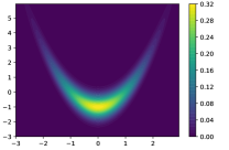
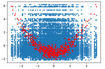

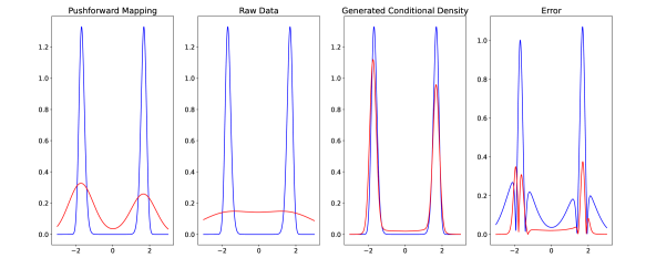
The right panel of Figure 1 plots the samples generated by pushing forward the product reference samples through the composed map . At the end of the algorithm, the push-forward condition should be satisfied. As a result, the push-forward should match the joint samples, as seen with the close match between the green and red samples. By Theorem 2.4 in Baptista et al. (2023), we can then use these maps to sample the conditional distribution for any . Figure 2 plots the approximate density (using a kernel density estimator) of the push-forward samples with for the conditioning variable . In comparison to the conditionals of a kernel density estimator of the joint samples from or , we observe close agreement with the true multi-modal conditional density for . We note that for invertible mappings , the change-of-variables formula can also be used to approximate the conditional density after learning the flow.
5.2 Lotka–Volterra dynamical system
In this section we apply Algorithm 1 to estimate static parameters in the Lotka–Volterra population model given noisy realizations of the states over time. The model describes the populations of prey and predator species, respectively. The populations for times solve the nonlinear coupled ODEs
| (15) |
with the initial conditional , where are unknown parameters. The parameters are initially distributed according to a log-normal prior distribution given by with . We simulate the ODE for time units and observe the state values every time units with independent and additive log-normal noise, i.e., for with . Figure 3 presents the two states in solid lines for the parameter and an observation drawn from the likelihood model in circles. The main reason for choosing this model to test the procedure described in Section 4 is that the likelihood model is known in closed form and thus the results can be compared to MCMC sampling procedures, the gold standard for Bayesian inference methods. In this experiment we learned the flow using only samples from the joint distribution.
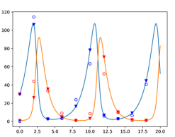
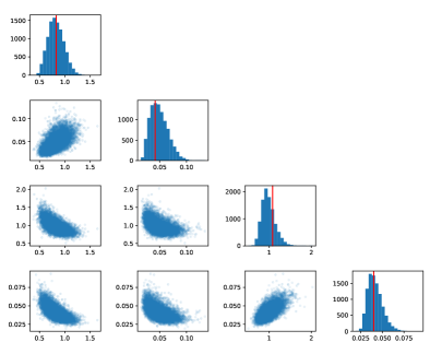
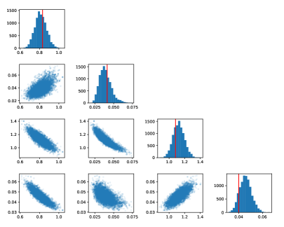
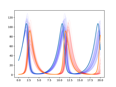
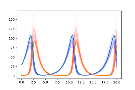
Figure 4 compares one and two-dimensional projections of the approximate posterior distribution for the parameters obtained with our procedure (left) and with MCMC (on the right). The red vertical line represents the exact value of the parameters used to generate the trajectory in Figure 3. For each approximation, we obtain the 30 most significant posterior samples, which are closest to the empirical posterior mean in the Euclidean norm. For each parameter, we find the corresponding state trajectories by solving the ODEs in (15). The states obtained with the flow and with MCMC are compared in the left and right of Figure 5 respectively. The posterior predictive states give a visual representation of the uncertainty arising from estimating the true parameter given noisy observations. As expected, the MCMC method displays lower uncertainty in the trajectories due to its use of the exact likelihood model. This is particularly noticeable for larger values of the populations where the effect of the noise on the sampled data (i.e., the difference between the circle and triangle markers in Figure 3) has a larger effect than during time intervals where and are nearly constant.
6 Conclusions and future work
This work presents a generative flow model for Bayesian inference where samples of the posterior distribution are generated by pushing forward prior samples through a composition of maps. Finding the flow is entirely data-driven and it is based on the theory of optimal transport (OT) with a weighted cost function. This cost yields transport maps with a block-triangular structure, which are are suitable for conditional sampling. The algorithm’s performance is illustrated on a two dimensional synthetic example and a Bayesian inference problem involving nonlinear ODEs. The advantage of this approach over state-of-the-art algorithms that seek OT maps for conditional sampling is that it only relies on pure minimization steps at each step of the flow rather than solving more challenging min-max optimization problems. The flow is constructed through elementary maps that, acting locally around where the samples are concentrated, gradually push forward the prior to the posterior distribution. Future work includes the possibility of enlarging the feature space for each map by means of projections into reproducing Kernel Hilbert spaces in a similar spirit to Chewi et al. (2020), as well as adapting the features to exploit low-dimensional structure between the reference and target distributions as in Brennan et al. (2020).
Acknowledgements
This work was done as part of the 2022 Polymath Junior summer undergraduate research program, supported by the NSF REU program under award DMS-2218374. RB gratefully acknowledges support from the US Department of Energy AEOLUS center (award DE-SC0019303), the Air Force Office of Scientific Research MURI on “Machine Learning and Physics-Based Modeling and Simulation” (award FA9550-20-1-0358), and a Department of Defense (DoD) Vannevar Bush Faculty Fellowship (award N00014-22-1-2790).
References
- Adler and Öktem [2018] J. Adler and O. Öktem. Deep bayesian inversion. arXiv preprint arXiv:1811.05910, 2018.
- Amos et al. [2017] B. Amos, L. Xu, and J. Z. Kolter. Input convex neural networks. In International Conference on Machine Learning, pages 146–155. PMLR, 2017.
- Arjovsky et al. [2017] M. Arjovsky, S. Chintala, and L. Bottou. Wasserstein generative adversarial networks. In International conference on machine learning, pages 214–223. PMLR, 2017.
- Baptista et al. [2020] R. Baptista, Y. Marzouk, and O. Zahm. On the representation and learning of monotone triangular transport maps. arXiv preprint arXiv:2009.10303, 2020.
- Baptista et al. [2023] R. Baptista, B. Hosseini, N. B. Kovachki, and Y. Marzouk. Conditional sampling with monotone GANs: from generative models to likelihood-free inference. arXiv preprint arXiv:2006.06755, 2023.
- Barber et al. [2015] S. Barber, J. Voss, and M. Webster. The rate of convergence for approximate Bayesian computation. Electronic Journal of Statistics, 9(1):80 – 105, 2015.
- Batzolis et al. [2021] G. Batzolis, J. Stanczuk, C.-B. Schönlieb, and C. Etmann. Conditional image generation with score-based diffusion models. arXiv preprint arXiv:2111.13606, 2021.
- Blei et al. [2017] D. M. Blei, A. Kucukelbir, and J. D. McAuliffe. Variational inference: A review for statisticians. Journal of the American statistical Association, 112(518):859–877, 2017.
- Brenier [1991] Y. Brenier. Polar factorization and monotone rearrangement of vector-valued functions. Communications on pure and applied mathematics, 44(4):375–417, 1991.
- Brennan et al. [2020] M. Brennan, D. Bigoni, O. Zahm, A. Spantini, and Y. Marzouk. Greedy inference with structure-exploiting lazy maps. Advances in Neural Information Processing Systems, 33:8330–8342, 2020.
- Bunne et al. [2022] C. Bunne, A. Krause, and M. Cuturi. Supervised training of conditional monge maps. Advances in Neural Information Processing Systems, 35:6859–6872, 2022.
- Carlier et al. [2010] G. Carlier, A. Galichon, and F. Santambrogio. From knothe’s transport to brenier’s map and a continuation method for optimal transport. SIAM Journal on Mathematical Analysis, 41(6):2554–2576, 2010.
- Carlier et al. [2016] G. Carlier, V. Chernozhukov, and A. Galichon. Vector quantile regression: An optimal transport approach. Annals of Statistics, 44(3):1165–1192, 2016.
- Chartrand et al. [2009] R. Chartrand, B. Wohlberg, K. Vixie, and E. Bollt. A gradient descent solution to the Monge-Kantorovich problem. Applied Mathematical Sciences, 3(22):1071–1080, 2009.
- Chewi et al. [2020] S. Chewi, T. Le Gouic, C. Lu, T. Maunu, and P. Rigollet. Svgd as a kernelized Wasserstein gradient flow of the chi-squared divergence. Advances in Neural Information Processing Systems, 33:2098–2109, 2020.
- Cranmer et al. [2020] K. Cranmer, J. Brehmer, and G. Louppe. The frontier of simulation-based inference. Proceedings of the National Academy of Sciences, 117(48):30055–30062, 2020.
- Cuturi [2013] M. Cuturi. Sinkhorn distances: Lightspeed computation of optimal transport. Advances in neural information processing systems, 26, 2013.
- Figalli and Glaudo [2021] A. Figalli and F. Glaudo. An Invitation to Optimal Transport, Wasserstein Distances, and Gradient Flows. EMS Press, 2021. 10.4171/ETB/22.
- Gangbo [1994] W. Gangbo. An elementary proof of the polar factorization of vector-valued functions. Archive for rational mechanics and analysis, 128:381–399, 1994.
- Grathwohl et al. [2018] W. Grathwohl, R. T. Chen, J. Bettencourt, I. Sutskever, and D. Duvenaud. FFJORD: Free-form continuous dynamics for scalable reversible generative models. arXiv preprint arXiv:1810.01367, 2018.
- Greenberg et al. [2019] D. Greenberg, M. Nonnenmacher, and J. Macke. Automatic posterior transformation for likelihood-free inference. In International Conference on Machine Learning, pages 2404–2414. PMLR, 2019.
- Gu et al. [2022] H. Gu, P. Birmpa, Y. Pantazis, L. Rey-Bellet, and M. A. Katsoulakis. Lipschitz regularized gradient flows and latent generative particles. arXiv preprint arXiv:2210.17230, 2022.
- Knothe [1957] H. Knothe. Contributions to the theory of convex bodies. Michigan Mathematical Journal, 4(1):39–52, 1957.
- Kobyzev et al. [2020] I. Kobyzev, S. J. Prince, and M. A. Brubaker. Normalizing flows: An introduction and review of current methods. IEEE transactions on pattern analysis and machine intelligence, 43(11):3964–3979, 2020.
- Liu et al. [2021] S. Liu, X. Zhou, Y. Jiao, and J. Huang. Wasserstein generative learning of conditional distribution. arXiv preprint arXiv:2112.10039, 2021.
- Lueckmann et al. [2019] J.-M. Lueckmann, G. Bassetto, T. Karaletsos, and J. H. Macke. Likelihood-free inference with emulator networks. In Symposium on Advances in Approximate Bayesian Inference, pages 32–53. PMLR, 2019.
- Makkuva et al. [2020] A. Makkuva, A. Taghvaei, S. Oh, and J. Lee. Optimal transport mapping via input convex neural networks. In International Conference on Machine Learning, pages 6672–6681. PMLR, 2020.
- Marzouk et al. [2016] Y. Marzouk, T. Moselhy, M. Parno, and A. Spantini. Sampling via measure transport: An introduction. In Handbook of Uncertainty Quantification, pages 1–41. Springer International Publishing, Cham, 2016. ISBN 978-3-319-11259-6. 10.1007/978-3-319-11259-6_23-1.
- Mirza and Osindero [2014] M. Mirza and S. Osindero. Conditional generative adversarial nets. arXiv preprint arXiv:1411.1784, 2014.
- Nadaraya [1964] E. A. Nadaraya. On estimating regression. Theory of Probability & Its Applications, 9(1):141–142, 1964.
- Nott et al. [2018] D. J. Nott, V. M.-H. Ong, Y. Fan, and S. Sisson. High-dimensional ABC. In Handbook of Approximate Bayesian Computation, pages 211–241. Chapman and Hall/CRC, 2018.
- Onken et al. [2021] D. Onken, S. W. Fung, X. Li, and L. Ruthotto. OT-flow: Fast and accurate continuous normalizing flows via optimal transport. In Proceedings of the AAAI Conference on Artificial Intelligence, volume 35(10), pages 9223–9232, 2021.
- Papamakarios et al. [2021] G. Papamakarios, E. Nalisnick, D. J. Rezende, S. Mohamed, and B. Lakshminarayanan. Normalizing flows for probabilistic modeling and inference. The Journal of Machine Learning Research, 22(1):2617–2680, 2021.
- Peyré et al. [2019] G. Peyré, M. Cuturi, et al. Computational optimal transport: With applications to data science. Foundations and Trends® in Machine Learning, 11(5-6):355–607, 2019.
- Pooladian and Niles-Weed [2021] A.-A. Pooladian and J. Niles-Weed. Entropic estimation of optimal transport maps. arXiv preprint arXiv:2109.12004, 2021.
- Rezende and Mohamed [2015] D. Rezende and S. Mohamed. Variational inference with normalizing flows. In International conference on machine learning, pages 1530–1538. PMLR, 2015.
- Robert et al. [1999] C. P. Robert, G. Casella, and G. Casella. Monte Carlo statistical methods, volume 2. Springer, 1999.
- Rosenblatt [1952] M. Rosenblatt. Remarks on a multivariate transformation. The annals of mathematical statistics, 23(3):470–472, 1952.
- Ruthotto and Haber [2021] L. Ruthotto and E. Haber. An introduction to deep generative modeling. GAMM-Mitteilungen, 44(2):e202100008, 2021.
- Saharia et al. [2022] C. Saharia, J. Ho, W. Chan, T. Salimans, D. J. Fleet, and M. Norouzi. Image super-resolution via iterative refinement. IEEE Transactions on Pattern Analysis and Machine Intelligence, 2022.
- Santambrogio [2015] F. Santambrogio. Optimal transport for applied mathematicians. Birkäuser, NY, 55(58-63):94, 2015.
- Sisson et al. [2018] S. A. Sisson, Y. Fan, and M. Beaumont. Handbook of approximate Bayesian computation. CRC Press, 2018.
- Spantini et al. [2022] A. Spantini, R. Baptista, and Y. Marzouk. Coupling techniques for nonlinear ensemble filtering. SIAM Review, 64(4):921–953, 2022.
- Tabak and Turner [2013] E. G. Tabak and C. V. Turner. A family of nonparametric density estimation algorithms. Communications on Pure and Applied Mathematics, 66(2):145–164, 2013.
- Tabak and Vanden-Eijnden [2010] E. G. Tabak and E. Vanden-Eijnden. Density estimation by dual ascent of the log-likelihood. Communications in Mathematical Sciences, 8(1):217–233, 2010.
- Taghvaei and Hosseini [2022] A. Taghvaei and B. Hosseini. An optimal transport formulation of Bayes’ law for nonlinear filtering algorithms. In 2022 IEEE 61st Conference on Decision and Control (CDC), pages 6608–6613. IEEE, 2022.
- Trigila and Tabak [2016] G. Trigila and E. G. Tabak. Data-driven optimal transport. Communications on Pure and Applied Mathematics, 69(4):613–648, 2016.
- Trippe and Turner [2017] B. L. Trippe and R. E. Turner. Conditional density estimation with Bayesian normalising flows. In Second workshop on Bayesian Deep Learning, 2017.
- Uscidda and Cuturi [2023] T. Uscidda and M. Cuturi. The monge gap: A regularizer to learn all transport maps. arXiv preprint arXiv:2302.04953, 2023.
- Villani et al. [2009] C. Villani et al. Optimal transport: old and new, volume 338. Springer, 2009.
- Watson [1964] G. S. Watson. Smooth regression analysis. Sankhyā: The Indian Journal of Statistics, Series A, pages 359–372, 1964.
- Wehenkel and Louppe [2019] A. Wehenkel and G. Louppe. Unconstrained monotonic neural networks. Advances in neural information processing systems, 32, 2019.
- Winkler et al. [2019] C. Winkler, D. Worrall, E. Hoogeboom, and M. Welling. Learning likelihoods with conditional normalizing flows. arXiv preprint arXiv:1912.00042, 2019.
Appendix A Map parametrization and simulation details
In this section we discuss our parameterization for the elementary potential functions that are used in the numerical experiments of Section 5.
In this work we selected the features to be inverse multiquadric kernels or radially-symmetric kernels of the form
| (16) |
where is the bandwidth and is the radius for some center point . This choice aligns with the approach presented in the first modern version of normalizing flows [Tabak and Turner, 2013], in which the features apply local expansions or contractions of the sample points around the centers .
Once the functional form of the kernels is prescribed, the elementary potential function is completely defined by the choice for the bandwidths and the centers . In our numerical experiments, we selected the centers uniformly at random from the samples of the reference distribution and the samples of the joint (target) distribution. For problems with high-dimensional parameters and observations, such as the Lotka-Volterra example in Section 5.2, we found that adapting the random sampling for the centers improves the speed of convergence of Algorithm 1. In particular, we selected the observation location of the center points to be near the particular observation of interest, , more frequently. This choice refines the map pushing forward to around , which is the map used to sample the target conditional .
Lastly, the bandwidth is chosen according to the rule of thumb described in Trigila and Tabak [2016]. That is,
| (17) |
where and are kernel density estimates (KDE) of the reference and the target distributions, respectively. The rationale behind (17) is to have kernels with a larger bandwidth where there are fewer samples of the reference and the target distributions, and with a smaller bandwidth that can finely resolve the density in regions of the domain where the distributions are more concentrated. Given that the kernel estimator is only needed to compute the scalar bandwidth, they are not meant to be very accurate and updated at every step of the algorithm. In this work, the target density is time independent and hence its KDE is computed only once at the beginning of the procedure. The KDE of the reference distribution is instead updated after every 200 steps of the algorithm. The scalar is a problem dependent parameter that can be either set to a fixed value (e.g., in our experiments) or selected via cross-validation.
To reduce the impact of the specific bandwidth adopted in our procedure, we further multiplied the value of in (17) by a time dependent constant , which decreases as the algorithm advances. In particular, at the beginning of the experiment, the radius of influence of the kernels (i.e., features that result in local expansions or contractions) are set to be large in order to cover the entire domain containing the samples of . As the simulation advances, we gradually decrease the value of to produce a more localized action of the elementary maps. In our experiments we chose
with the parameters taken to be , and , where is the maximum number of steps we allow the algorithm to complete.
Appendix B Derivation of the Jacobian and Hessian
In this section we derive expressions for the Jacobian and Hessian of the empirical objective functional in (13) with respect to the parameters of the elementary potential function . To compute these derivative, in Proposition 1 we first derive an expression for the c-transform of the parametric potential function appearing inside the objective functional.
Proposition 1.
For the cost function let be the c-transform of the differentiable function where . Then, has an second-order asymptotic expansion in given by
| (18) |
Proof.
Let be the optimal that attains the minimum value for the c-transform, i.e., . For a differentiable function , the optimal value satisfies . Thus, for the parametric expansion we have the condition , which defines an implicit function for in terms of .
Substituting the expression for in the c-transform gives us
| (19) |
where depends on . A first-order Taylor series expansion of each feature in the first term of (19) around yields the following second-order asymptotic expansion in the coefficients
Similarly, a first-order Taylor series expansion of each feature in the second term of (19) around yields the asymptotic expansion
Substituting these expansions in (19), we arrive at the second-order expansion in (18) after collecting the quadratic terms in and using the definition of the rescaled gradient. ∎
Using the result of Proposition 1, a second-order asymptotic expansion in for the empirical objective functional is given by
Computing the first and second derivatives of the functional above with respect to each coefficient and evaluating the result at results in the Jacobian and Hessian presented in Section 4.