Towards a self-consistent model of the convective core boundary in upper-main-sequence stars

There is strong observational evidence that convective cores of intermediate-mass and massive main-sequence stars are substantially larger than standard stellar-evolution models predict. However, it is unclear what physical processes cause this phenomenon or how to predict the extent and stratification of stellar convective boundary layers. Convective penetration is a thermal-time-scale process that is likely to be particularly relevant during the slow evolution on the main sequence. We use our low-Mach-number Seven-League Hydro (SLH) code to study this process in 2.5D and 3D geometries. Starting with a chemically homogeneous model of a $15$ M_⊙ zero-age main-sequence star, we construct a series of simulations with the luminosity increased and opacity decreased by the same factor ranging from $10^{3}$ to $10^{6}$. After reaching thermal equilibrium, all of our models show a clear penetration layer. Its thickness becomes statistically constant in time and it is shown to converge upon grid refinement. As the luminosity is decreased, the penetration layer becomes nearly adiabatic with a steep transition to a radiative stratification. This structure corresponds to the adiabatic ,,step overshoot” model often employed in stellar-evolution calculations. The thickness of the penetration layer slowly decreases with decreasing luminosity. Depending on how we extrapolate our 3D data to the actual luminosity of the initial stellar model, we obtain penetration distances ranging from $0.09$ to $0.44$ pressure scale heights, which are broadly compatible with observations.

1 Introduction

Numerous observations strongly suggest that the convective, hydrogen-burning cores of intermediate-mass and massive stars are larger than the linear-stability criteria of Schwarzschild and Ledoux (see e.g. Kippenhahn et al., 2012) predict. The evidence has traditionally been based on colour-magnitude diagrams of open clusters (e.g. Maeder & Mermilliod, 1981; Demarque et al., 1994) and observations of eclipsing binary systems (Claret & Torres, 2016, and references therein). More recently, core sizes have also been measured using asteroseismology (Aerts, 2013; Anders & Pedersen, 2023, and references in the latter), confirming the large core radii. The size of the mixed core on the main sequence influences stellar lifetimes as well as stellar structure and evolution in later evolutionary stages.

The umbrella term ,,convective overshooting” has traditionally been used to describe all physical processes that contribute to extending stellar convection zones, although the terms ,,convective penetration” and ,,convective boundary mixing” are also used, often interchangeably. We reserve the term ,,convective penetration” for a process that is fast enough to change the thermal stratification beyond the Schwarzschild boundary (see also Anders & Pedersen, 2023). Classical one-dimensional stellar evolution theory resorts to simple parametric prescriptions for such processes, which severely limits the predictive power of current stellar-evolution models. Two prescriptions are particularly popular (see e.g. Kippenhahn et al., 2012): ,,step overshoot” and ,,exponentially decaying diffusion”. The first represents an approximate model of convective penetration. It assumes that mixing essentially as fast as that in the formally convective layer extends some distance beyond the Schwarzschild boundary, making the stratification chemically homogeneous and adiabatic with a discontinuous transition to the radiative stratification. The other prescription describes chemical mixing using a diffusion coefficient decreasing exponentially with the distance from the convective boundary while assuming that the thermal stratification remains radiative. Both prescriptions involve a free parameter that describes the radial extent of the mixing.

Core convection is characterised by low Mach numbers (of order $10^{-4}$ to $10^{-3}$) in main-sequence stars. The overlying stratification is so stable that it stops the slow convective flows within a tiny fraction of the pressure scale height (Roxburgh, 1965; Saslaw & Schwarzschild, 1965). This kind of dynamical ,,overshoot” cannot reconcile stellar-evolution models with the observations mentioned above. Three-dimensional (3D), hydrodynamic simulations show that mass entrainment is possible even at stiff convective boundaries (e.g. Meakin & Arnett, 2007; Woodward et al., 2015; Horst et al., 2021). However, simulations of core convection on the main sequence predict unrealistically high mass entrainment rates (Meakin & Arnett, 2007; Gilet et al., 2013; Herwig et al., 2023), suggesting that the observed fast entrainment is just a transient phenomenon. Indeed, most of such simulations do not include radiative diffusion, making it impossible to sustain the expected stellar structure with a convective core and a radiative envelope on long time scales. Particularly relevant is the thermal time scale, on which heat transport processes, including convective penetration, set the thermal structure of the star.

Processes occurring on the thermal time scale can be qualitatively described in terms of how they affect the radial profile of entropy. Both nuclear burning and hydrodynamic entrainment of high-entropy material from the radiative envelope increase the mean entropy of the mixed core. On the other hand, radiative diffusion carries energy outwards, decreasing the core entropy. It is reasonable to assume that the two processes reach equilibrium and the core stops changing its size on the thermal time scale (ignoring slow changes in chemical composition occurring on the nuclear time scale). Somewhat surprisingly, one can put analytical constraints on how large the convective core can be in the equlibrium state. Roxburgh (1978, 1989) averages the 3D equations of fluid motion and radiative heat transport in space and time and, assuming statistically stationary convection, he derives a simple integral criterion for the size of the convective core,

$$\int_{V}\left(\overline{F}-\overline{\Gamma}\right)\frac{1}{T_{0}^{2}}\frac{\mathrm{d}T_{0}}{\mathrm{d}r}\mathrm{d}V=\int_{V}\frac{\Phi_{0}}{T_{0}}\mathrm{d}V,$$ (1)

where $\overline{F}$ and $\overline{\Gamma}$ are the mean radial components of the radiative flux and of the energy flux from nuclear sources, respectively, $T$ is the temperature, and $\Phi$ the dissipation rate of kinetic energy. The subscript ,,$0$” refers to the mean state and the integration is performed over volume $V$ of the core. The radial profile of the dissipation rate $\Phi_{0}$ depends on details of the turbulent convective flow. Neglecting this term, Roxburgh obtains the maximum possible core mass, concluding that it can be substantially larger than the mass inside the formal Schwarzschild boundary. Roxburgh (1978, 1989) as well as Zahn (1991) argue that the whole core must be nearly adiabatic, including its extension beyond the Schwarzschild boundary now known as the ,,convective penetration layer”. However, the thickness of this layer cannot be further constrained without constraining the turbulent dissipation rate.

Multi-dimensional hydrodynamic simulations can encompass all physical processes needed to compute detailed models of penetrative convection. However, the thermal time scale associated with typical stellar convective layers is orders of magnitude longer than the convective turnover time scale and the only way to to obtain thermally relaxed simulations is to boost the heat flux by several orders of magnitude. Using this technique, a few research groups have recently managed to approach the thermal time scale and to observe the formation of a convective penetration layer in various stellar environments (Hotta, 2017; Käpylä, 2019; Baraffe et al., 2023; Blouin et al., 2023; Mao et al., 2023). Baraffe et al. (2023) run 2D simulations of a range of main-sequence stars with convective cores but only one of their simulations (of a $3$ M_⊙ star) uses sufficient luminosity boosting for the penetration layer to start approaching thermal equilibrium. The growth of the convective core of a $25$ M_⊙ main-sequence star slows down on the thermal time scale in the 3D simulations of Mao et al. (2023) but the core does not stop growing. This might be a consequence of continued chemical mixing in the simulation. In the simpler case of a chemically homogeneous stratification, Anders et al. (2022) show that the penetration layer stops growing on a sufficiently long time scale, reaching a statistically stationary state. However, their simulations use a simplified stratification rather than a realistic stellar model and their use of the Boussinesq approximation eliminates any effects of compressibility, which may be important in the strongly stratified stellar interior.

Our study focuses on thermal aspects of the stellar convective-penetration problem. We eliminate compositional effects by using a realistic model of a $15$ M_⊙ zero-age main sequence (ZAMS) star. Employing the standard approach of luminosity boosting, we show that a penetration layer forms at the core boundary and stops growing on the thermal time scale. We measure the core size in the thermally relaxed state and extrapolate towards the star’s nominal luminosity. We run both 2.5D and 3D simulations using our fully compressible, low-Mach number Seven-League Hydro (SLH) code (Miczek, 2013; Edelmann, 2014; Edelmann et al., 2021) to explore both the limit of low turbulent dissipation as expected in two-dimensional convection and assumed by Roxburgh as well as the more realistic case of 3D turbulent convection.

We describe our 1D initial stellar model in Sections 2.1 and 2.2. The numerical set-up of the 2.5D and 3D SLH simulations is detailed in Sect. 2.3. We use a simple numerical experiment to illustrate the importance of radiative diffusion in Sect. 3.1. Relevant properties of our 2.5D and 3D simulations and their numerical convergence are described in Sections 3.2–3.4. We then extrapolate the thickness of the penetration layer to the actual luminosity of the stellar model in Sect. 3.5. Our results are summarised and discussed in Sect. 4.

2 Methods

2.1 1D stellar model

We use version $15140$ of the stellar-evolution code MESA (Paxton et al., 2011, 2013, 2015, 2018, 2019; Jermyn et al., 2023) to compute a model of a $15\mathrm{M}_{\odot}$ star with a metallicity of $Z=0.02$ at the ZAMS. The evolution model is stopped at the age of $7.96\times 10^{4}$ yr, when the convective core has fully developed and the star has reached thermal equlibrium. At this stage, the central hydrogen mass fraction has decreased by $0.156\%$ from its initial value of $0.700$. The star’s radius and luminosity are $R_{\star}=3.47\times 10^{11}$ cm ($4.98\,R_{\odot}$) and $L_{\star}=7.49\times 10^{37}$ erg s^-1 ($1.95\times 10^{4}\,L_{\odot}$), respectively. The model does not include any convective ,,overshoot” or penetration. The latter evolves in our multi-dimensional models in a self-consistent way. The Schwarzschild boundary of the core is located at $8.74\times 10^{10}$ cm ($0.252\,R_{\star}$). The MESA inlist for the model as well as the resulting profile file are available on Zenodo.

2.2 Simplification of the initial 1D model

The MESA model contains a $0.093\%$ jump in the mean molecular weight at the core boundary because some hydrogen burning occurred during the initial thermal adjustment of the model. We remove this step by applying the central value of the mean molecular weight $\mu=0.6174$ to the whole star in order to eliminate any compositional effects. To obtain an initial condition for multidimensional simulations, we re-integrate the hydrostatic stratification assuming that the difference between the actual temperature gradient $\nabla$ and the adiabatic gradient $\nabla_{\mathrm{ad}}$ is given by the MESA model everywhere but in the convective core, where it is set to zero. The equation of state used in this integration process as well as in the hydrodynamic simulations described below accounts for a mixture of fully ionised, monatomic gas and radiation. The radial profile of gravitational acceleration is interpolated from the MESA model without any modification. The resulting profiles of the pressure $p$ as well as specific entropy $s$ closely match those of the original MESA model, see Fig. 1.

Figure 1 also shows the profiles of opacity $\kappa$ and energy generation rate per unit volume $\rho\varepsilon_{\mathrm{nuc}}$. The opacity is simply interpolated without any modification. The profile of the energy generation rate is for reasons of computational efficiency modelled using the fitting function

$$\rho\varepsilon_{\mathrm{nuc}}=\cases{4}.135\times 10^{5}\exp\left[-\frac{r^{2}}{(3.15\times 10^{10}\,\mathrm{cm})^{2}}\right]\,\mathrm{erg\,cm}^{-3}\ \mathrm{for}\ r<r_{0},\\ 0\ \mathrm{otherwise},{}$$ (2)

where $r_{0}=8.736\times 10^{10}\,\mathrm{cm}$ is the radius of the initial core boundary. This profile is almost indistinguishable from that provided by MESA for $r<r_{0}$, see Fig. 1. There is a small-amplitude spike in the energy generation rate at $r=r_{0}$ in the MESA model due to a slight change in composition. We do not model this spike. Additionally, our 2.5D and 3D simulations have a central cut-out with a radius of $8.7\times 10^{9}$ cm ($0.025\,R_{\star}$, see Sect. 2.3 for details). Taking into account all of these effects, the total luminosity of the modified model is $5.5\%$ lower than that of the original MESA model.

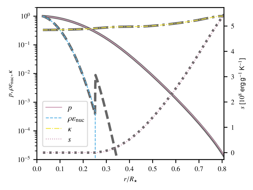
Figure 1: Stratification of the pressure $p$, energy generation rate per unit volume $\rho\varepsilon_{\mathrm{nuc}}$, opacity $\kappa$, and specific entropy $s$ in the MESA model (thick grey lines) and in the SLH model at $t=0$ (thin coloured lines). The profiles of $p$ and $\rho\varepsilon_{\mathrm{nuc}}$ are normalised such that their maximum values are unity. The entropy of the convective core is set to $0$. The jump in $\rho\varepsilon_{\mathrm{nuc}}$ at the boundary of the fully-mixed core is caused by a slight change in chemical composition, which is neglected in the SLH model.

2.3 2.5D and 3D simulations

As mentioned in Sect. 1, the time and length scales involved in the process of convective penetration in stars make the problem prohibitively costly for multidimensional hydrodynamic simulations. We illustrate this in Table 1, which is based on results of our simulations (see Sect. 3 for details). The last row of the table is an extrapolation to our $15\,\mathrm{M}_{\odot}$ star’s actual parameters. The thermal time scale of the model is $5.9\times 10^{4}$ yr, which corresponds to $6.5\times 10^{5}$ convective turnover time scales. This is well beyond what can currently be achieved using multidimensional simulations. Additionally, we must consider the need to resolve the length scale of radiative diffusion on the turnover time scale. Table 1 shows that this length scale evaluated at the core boundary is only $0.4$ cell widths on a grid with $512$ radial grid cells. To marginally resolve it by $4$ cells, we would need a grid with ${\approx}\,5000$ radial cells, making the simulations extremely expensive.

We solve these problems by increasing the energy-generation rate by a boost factor $b$ ranging from $10^{3}$ to $10^{6}$, which shortens both the thermal and convective turnover time scales. We decrease the opacity by the same factor, which increases the thermal diffusion length scale. This choice also has the advantage that the radiative temperature gradient $\nabla_{\mathrm{rad}}$, which is proportional to the product of the luminosity and opacity, becomes independent of $b$ and the stratification of the radiative layer remains largely the same.

Table 1: Time and length scales for the $15\,\mathrm{M}_{\odot}$ ZAMS star.

$b$	$\tau_{\mathrm{th}}$ [yr]	$\tau_{\mathrm{conv}}$ [d]	$\tau_{\mathrm{th}}/\tau_{\mathrm{conv}}$	$l_{\mathrm{d}}/\Delta r_{512}$
$10^{6}$	$5.9\times 10^{-2}$	$7.5\times 10^{-1}$	$2.9\times 10^{1}$	$69$
$10^{5}$	$5.9\times 10^{-1}$	$1.4\times 10^{0}$	$1.5\times 10^{2}$	$29$
$10^{4}$	$5.9\times 10^{0}$	$2.6\times 10^{0}$	$8.1\times 10^{2}$	$12$
$10^{3}$	$5.9\times 10^{1}$	$5.0\times 10^{0}$	$4.3\times 10^{3}$	$5.0$
$10^{0}$	$5.9\times 10^{4}$	$3.3\times 10^{1}$	$6.5\times 10^{5}$	$0.4$

We use the SLH code to simulate the convective penetration process using the simplified 1D model as an initial condition. The code solves the following set of compressible, inviscid Euler equations with gravity and diffusive heat transport:

$$\partial_{t}\,\rho+\bm{\nabla}{\cdot}(\rho\bm{u}) =0,$$ (3)

$$\partial_{t}(\rho\bm{u})+\bm{\nabla}{\cdot}(\rho\bm{u}\otimes\bm{u}+p\bm{\mathbb{I}}) =\rho\bm{g},$$ (4)

$$\partial_{t}(\rho e_{\mathrm{t}})+\bm{\nabla}{\cdot}[(\rho e_{\mathrm{t}}+p)\bm{u}-\chi\bm{\nabla}T] =\rho\varepsilon_{\mathrm{nuc}},$$ (5)

where $\rho$, $\bm{u}$, $p$, $\bm{\mathbb{I}}$, $\bm{g}$, $\chi$, $T$, $\varepsilon_{\mathrm{nuc}}$ denote the density, velocity, pressure, unit tensor, gravity, thermal conductivity, temperature, and energy generation rate by nuclear reactions, respectively. The specific total energy $e_{\mathrm{t}}=e_{\mathrm{i}}+e_{\mathrm{k}}+\Psi$ includes internal energy $e_{\mathrm{i}}(\rho,T)$, kinetic energy $e_{\mathrm{k}}=\frac{1}{2}|\bm{u}|^{2}$, and a time-independent gravitational potential $\Psi$.

The equations are solved on two types of grids: 2.5D and 3D. Both of them match the spherical geometry of stars to suppress discretisation errors. The 3D grid is a spherical grid with uniform spacing in the radius $r$, polar angle (colatitude) $\vartheta$, and azimuthal angle (longitude) $\varphi$. The 2.5D grid is a polar grid with uniform spacing in $r$ and $\vartheta$ that describes a 3D spherical system with all variables constant in $\varphi$ (rotational symmetry around the polar axis). This results in a geometric source term in the numerical scheme, which is taken into account. The grids cover the radial range from $8.7\times 10^{9}$ cm ($0.025\,R_{\star}$) to $2.8\times 10^{11}$ cm ($0.808\,R_{\star}$). We limit the range of polar angles to $30^{\circ}\leq\vartheta\leq 150^{\circ}$ because the cell width in the azimuthal direction drops close to the polar axis, severely limiting the time-step length. In the 3D case, we include azimuthal angles in the range $-60^{\circ}\leq\varphi\leq 60^{\circ}$.

To judge numerical convergence of our results, we run simulations with each boost factor $b$ on a range of grids. The number of radial grid cells is $N_{r}\in(128,256,512,1024)$ in 2.5D and $N_{r}\in(128,192,256)$ in 3D. The only exception is that we do not include a 2.5D simulation with $b=10^{3}$ and $N_{r}=1024$, which would be too costly. The number of cells in each of the two angular directions is always $N_{r}/2$.

We impose reflective boundary conditions at all boundaries of the computational domain. The only exception is the outer radial boundary, where the temperature in the first ghost cell is set to the value given by the initial 1D model when and only when the radiative-diffusion term is computed. The reflective boundaries in the angular directions eliminate horizontal shear flows, which often become strong with periodic boundaries.

The SLH code is based on a finite-volume discretisation and offers both explicit and implicit time steppers via the method of lines. In this work, we use the ESDIRK23 implicit stepper (Hosea & Shampine, 1996). The bulk Mach numbers reported in Sect. 3.2 may suggest that the flows in some of our simulations are fast enough to be better suited for explicit time steppers. However, this impression is misleading. Even without considering radiative diffusion, the length of explicit time steps would be limited by the inner edge of the computational grid, where the sound speed is fastest and grid cells are narrowest in the angular directions. For this reason, implicit time steps can be $50$ to $80$ times longer than explicit ones even with the highest boost factor $b=10^{6}$. This ratio is of similar order as the cost-per-step ratio of the implicit to a comparable explicit stepper, making both approaches comparably expensive with $b=10^{6}$. However, fast radiative diffusion caused by low density at the outer edge of the simulation domain imposes much stricter time-step constraints. The ratio of the lengths of implicit to diffusion-limited explicit time steps in the 2.5D simulation with $b=10^{6}$ and computed on the $1024\times 512$ grid is ${\approx}\,5000$. Diffusion is much less constraining in simulations with $b=10^{3}$ but convection is so slow in those that than longest possible explicit time steps would be ${\approx}\,500$ times shorter than implicit steps. All in all, the implicit approach saves a significant amount of computing time.

We use unlimited parabolic reconstruction in space. Because the stratification spans five orders of magnitude in pressure (see Fig. 1), hydrostatic equilibrium requires a special treatment to suppress spurious flows caused by discretisation errors, see Edelmann et al. (2021) for details. Specifically, we use the well-balancing method of Berberich et al. (2021), later referred to as the ,,deviation method” by Edelmann et al. (2021). We further increase our resolving power by employing the low-Mach-number numerical flux function AUSM+-up of Liou (2006), which is much less dissipative than standard Riemann solvers in slow flows. We slightly modify the flux function as described by Edelmann et al. (2021). The modified flux uses the parameters $f_{a}=10^{-10}$ and $f_{a}^{p}=10^{-1}$ in the notation of the latter paper.

Because simulations of turbulence are statistical in nature, we take great care to quantify and take into account statistical variation in the data we extract from the simulations. We express statistical-variation ranges using $\pm 1\sigma$ intervals, where $\sigma$ is the uncorrected standard deviation of the statistical sample, unless mentioned otherwise.

3 Results

3.1 Importance of radiative diffusion

We start by demonstrating that the presence of radiative diffusion is essential for our simulations to reach a statistically stationary state. In Fig. 2, we compare two simulations performed with a boost factor of $10^{4}$ on a $256\times 128$ grid. The convective core keeps growing in the simulation that does not include radiative diffusion until, ultimately, the whole model becomes convective. This effect can be understood even without considering hydrodynamic mass entrainment. The heat source in the core keeps increasing the mean entropy of the mixed core. Whenever that entropy becomes greater than the entropy of a stably stratified layer atop the core, that layer gets mixed into the core. Ultimately, the entropy of the whole model becomes approximately the same and the star becomes fully convective. This process is further accelerated by the presence of strong internal gravity waves, which seem to induce some mixing and flatten the entropy profile close to the outer boundary of the computational domain (i.e. where the waves reach their maximum amplitude). On the other hand, changes to the entropy profile are much more subtle in the simulation with radiative diffusion, in which the initial outward propagation of the convective boundary stops early on and the simulation reaches a statistically stationary state. This is possible because radiative diffusion is sufficiently fast to transport entropy generated in the core through the radiative envelope. The heat then leaves the box owing to the constant-temperature outer boundary condition. This statistically stationary state can be maintained indefinitely because we do not model changes to the chemical composition of the core due to nuclear burning. We only discuss simulations with radiative diffusion in the rest of this section.

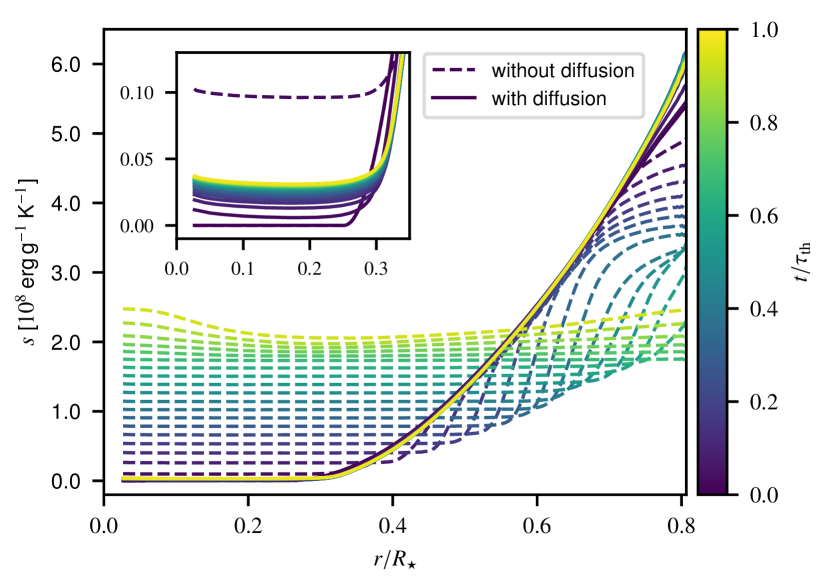
Figure 2: Time evolution of the radial profiles of the specific entropy $s$ in 2.5D simulations without and with radiative diffusion. Both simulations have $b=10^{4}$ and $N_{r}=256$. The profiles are shifted such that the entropy of the convective core is $0$ at $t=0$. Simulation time is given as a fraction of the thermal time scale $\tau_{\mathrm{th}}$ on the colour bar. Each curve, except for that showing the initial condition, corresponds to a time average over $0.05\tau_{\mathrm{th}}$.

3.2 Velocity field

The velocity field depends primarily on the boost factor $b$. This factor sets both convective velocity and efficiency. Because we scale $\kappa\propto b^{-1}$, the rate of radiative diffusion increases in proportion to $b$ and fluid parcels exchange increasing amounts of heat with their surroundings as they rise and sink in the convective core. This effect makes convection less efficient at transporting heat. Figure 3 shows the velocity field in 2.5D simulations with boost factors ranging from $10^{6}$ down to $10^{3}$. The velocity field in the core is dominated by large-scale vortices as typical of 2D convection. Small-scale motions are further suppressed by radiative damping. The structure of the convective flow is completely different in 3D, see Fig. 4. Instead of large vortices, we obtain a turbulent cascade from large to small scales as expected for 3D convection (without strong rotation or magnetic fields).

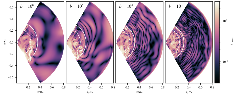
Figure 3: Velocity fields in 2.5D simulations with boost factors $b\in(10^{6},10^{5},10^{4},10^{3})$ performed on the $512\times 256$ grid. The velocity is normalised using the typical convective velocity $u_{\mathrm{conv}}$ as given by the scaling law shown in Fig. 6. The dashed and solid lines give the time-averaged radii of the Schwarzschild and convective boundaries, respectively. The simulations are shown at $t=0.5\tau_{\mathrm{th}}(b)$.

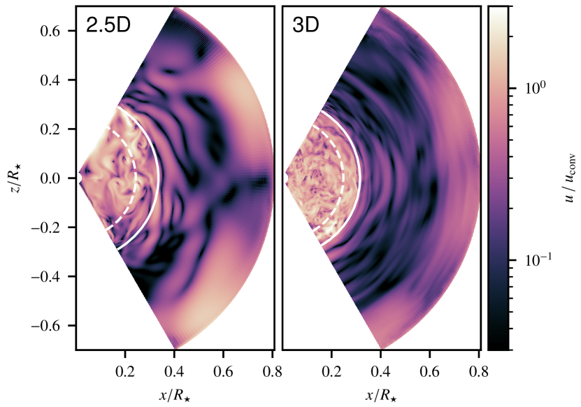
Figure 4: As Fig. 3 but comparing 2.5D and 3D simulations with a boost factor of $b=10^{5}$ performed on grids of $256\times 128$ and $256\times 128^{2}$ cells, respectively. In the 3D case, a slice with the spherical angle $\varphi=0$ is shown.

The convective core generates internal gravity waves (IGWs), which propagate through the radiative envelope. When we decrease the boost factor $b$, the convection becomes slower and it generates waves at lower temporal frequencies. Basic theory of linear IGWs (see e.g. Lighthill, 2001; Sutherland, 2010) predicts that a decrease in frequency corresponds to a decrease in the radial wavelength for the same horizontal wavelength. This effect is evident in Fig. 3 and it is further amplified by the dependence on $b$ of the radiative diffusivity, which filters out the shortest wavelengths.

The simulations in Fig. 3 are shown after a statistically stationary state has been reached. The figure also shows the radius of the convective boundary $r_{\mathrm{cb}}$ (solid lines), the exact definition of which we defer to the next section. For now, we only use it to measure convective velocity $u_{\mathrm{conv}}$. We define this quantity to be the the mass-weighted, root-mean-square (rms) velocity averaged between the inner boundary of the computational domain and the radius $r_{\mathrm{cb}}$ of the convective boundary. Figure 5 shows $u_{\mathrm{conv}}$ as a function of time, boost factor, grid resolution, and the dimensionality of the simulation. The convective velocity rapidly reaches a statistically stationary state. For each boost factor $b$, the velocity is not only statistically constant in time but it is also the same for 2.5D and 3D simulations and all grid resolutions. This is rather surprising since the structure of the convective flows differs substantially between 2.5D and 3D (Fig. 4). Although the same total energy flux has to be transported in both cases, the velocity is only one of several variables that contribute to the fluxes of enthalpy and kinetic energy. Indeed, numerical studies of stellar convection usually show faster convective velocities in 2D than in 3D with the same initial condition (Muthsam et al., 1995; Meakin & Arnett, 2007; Pratt et al., 2020; Horst et al., 2021). It is possible that the growth of convective instability is in our simulations limited by the same phenomenon in both geometries, which could be radiative damping or bouyancy braking in the penetration layer. More investigation is needed to disentangle these effects.

Convective velocity scales with $b^{1/3}$ in simulations of adiabatic convection (Jones et al., 2017; Cristini et al., 2019; Edelmann et al., 2019; Horst et al., 2021; Herwig et al., 2023). Our best-fit scaling is $u_{\mathrm{conv}}\propto b^{0.285\pm 0.002}$ for the four 2.5D simulations with $N_{r}=512$, see Fig. 6. The mean exponent of the scaling differs by $-26\sigma$ from the adiabatic value of $1/3$. To obtain a measure of statistical variation for each data point, we consider the convective velocities averaged over each of the $n_{\mathrm{bins}}=14$ time bins after the initial transient ($t>0.3\tau_{\mathrm{th}}$) as statistically independent measurements. The standard deviation of the average of all of the bins is then estimated to be $\sigma=\sigma_{\mathrm{series}}/n_{\mathrm{bins}}^{1/2}$, where $\sigma_{\mathrm{series}}$ is the standard deviation of the time series. We then compute $10^{5}$ statistical realisations of the scaling law assuming a normal distribution of statistical fluctuations, fit a power law to each of them, and compute the mean scaling and the statistical spread around the mean as a function of $b$. All 2.5D and 3D data points shown in Fig. 6 are statistically consistent with the scaling law. Our best estimate of convective velocity at the star’s nominal luminosity (i.e. $b=1$) is $(7.49\pm 0.13)\times 10^{4}$ cm s^-1. Taking the mass-weighted average sound speed $c_{\mathrm{ref}}=7.96\times 10^{7}$ cm s^-1 inside the initial Schwarzschild radius as a reference, we obtain a nominal Mach number of $(9.41\pm 0.16)\times 10^{-4}$. If we only fit the two lowest-luminosity 2.5D data points the resulting scaling exponent is $0.291\pm 0.004$, which is statistically consistent with the exponent based on the full 2.5D data set. Finally, if we only fit the two 3D data points we obtain a scaling exponent of $0.295\pm 0.006$, which differs by $-6.3\sigma$ from the adiabatic value of $1/3$ and is statistically consistent with the exponent based on the full 2.5D data set. The 3D-based scaling gives a convective velocity of $(6.65\pm 0.50)\times 10^{4}$ cm s^-1 at $b=1$, which is consistent with the 2.5D-based prediction. All of the 2.5D data points are also statistically consistent with the 3D-based scaling. It is possible that radiative damping makes the scaling shallower, although it is unclear why its exponent does not approach $1/3$ at low boost factors, i.e. when radiative diffusion becomes relatively slow in the core. One might also suspect numerical effects. However, Edelmann et al. (2021) demonstrate that the SLH code produces the expected $1/3$ velocity scaling for adiabatic convection down to Mach numbers of $2\times 10^{-4}$ in a star-like environment.

We define the convective turnover time scale as

$$\tau_{\mathrm{conv}}=\frac{2r_{\mathrm{cb}}}{u_{\mathrm{conv}}}.$$ (6)

For simplicity, we set $r_{\mathrm{cb}}=r_{\mathrm{Sb},0}+\alpha(b)H_{\mathrm{p,Sb},0}$ in this estimate, where the $r_{\mathrm{Sb},0}$ and $H_{\mathrm{p,Sb},0}$ are the radius of and pressure scale height at the Schwarzschild boundary in the initial MESA model, and we take the scaling law $\alpha(b)$ derived from our 2.5D simulations in Sect. 3.5 and shown in Fig. 12. The resulting values of $\tau_{\mathrm{conv}}$, summarised in Table 1, range from $0.75$ d at $b=10^{6}$ to $5.0$ d at $b=10^{3}$. Extrapolating to the nominal luminosity ($b=1$), we obtain $\tau_{\mathrm{conv}}=33$ d.

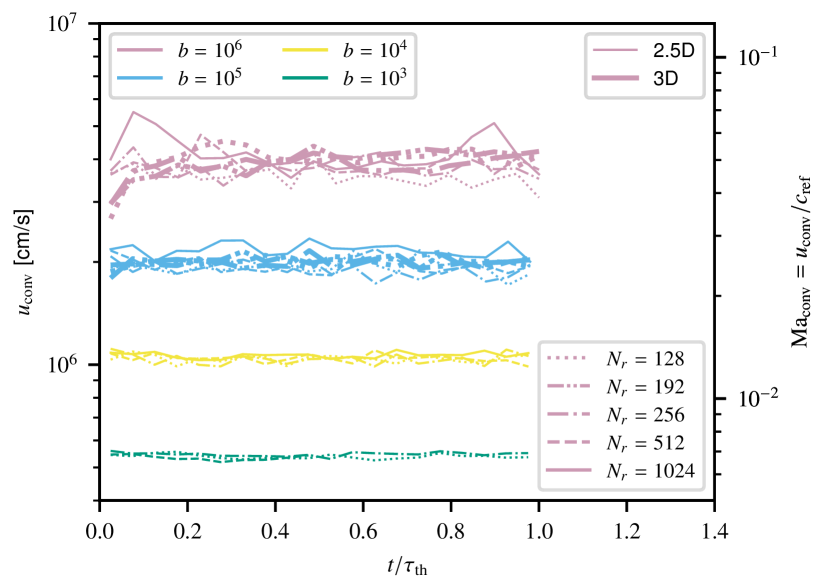
Figure 5: Time evolution of the convective velocity $u_{\mathrm{conv}}$ in all of our simulations with radiative diffusion. The time axis shows simulation time as a fraction of the thermal time scale $\tau_{\mathrm{th}}(b)$. Each data point corresponds to a time average over $0.05\tau_{\mathrm{th}}$. The right vertical axis shows the corresponding Mach numbers computed using the reference sound speed $c_{\mathrm{ref}}=7.96\times 10^{7}$ cm s^-1.

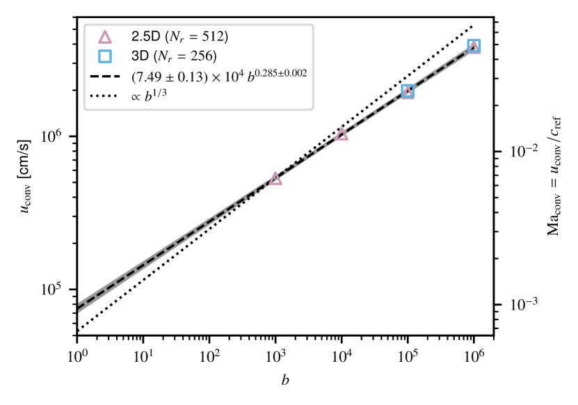
Figure 6: Dependence of the convective velocity $u_{\mathrm{conv}}$ on the boost factor $b$. The right vertical axis shows the corresponding Mach numbers computed using the reference sound speed $c_{\mathrm{ref}}=7.96\times 10^{7}$ cm s^-1. Statistical-variation ranges for the individual data points are smaller than the markers and not shown. A straight line is fitted to the 2.5D data points using the Monte-Carlo procedure described in Sect. 3.2. The grey shading shows the $3\sigma$ statistical-variation interval around the mean fit. Parameters of the scaling law are given in the legend. The usual adiabatic scaling $u_{\mathrm{conv}}\propto b^{1/3}$ is also shown for comparison.

3.3 Thermal evolution

In all of our simulations, we initially observe rapid growth in the size of the convective core. To illustrate this, we plot in Fig. 7 the time evolution of the actual and radiative temperature gradients $\nabla$ and $\nabla_{\mathrm{rad}}$ in the 2.5D simulation with $b=10^{4}$ and $N_{r}=1024$. The gradients are normalised using the adiabatic temperature gradient $\nabla_{\mathrm{ad}}$, so the formal Schwarzschild boundary is located at the radius $r_{\mathrm{Sb}}$ where $\nabla_{\mathrm{rad}}/\nabla_{\mathrm{ad}}=1$. The Schwarzschild boundary moves slightly inwards over the thermal time scale. In contrast, the growth in the radial extent of the nearly-adiabatic core is much more pronounced. A convective-penetration layer develops above the Schwarzschild boundary. The temperature gradient in the bulk of this layer is slightly sub-adiabatic but significantly super-radiative, i.e. the total flux could in principle be transported by radiative diffusion but vigorous convection is still present. The outward propagation rate of the convective boundary drops rapidly after ${\approx}\,0.1\tau_{\mathrm{th}}$ and a statistically stationary state seems to have been reached by ${\approx}\,(0.2-0.3)\tau_{\mathrm{th}}$. There is some slight late-time adjustment of the temperature gradient near the outer boundary of the simulation box. However, the layer affected by it is sufficiently far out to not influence the penetration distance.

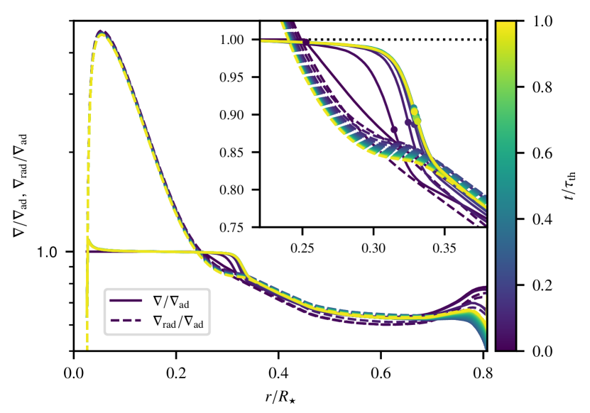
Figure 7: Time evolution of the radial profiles of the actual and radiative temperature gradients $\nabla$ and $\nabla_{\mathrm{rad}}$, respectively, in the 2.5D simulation with $b=10^{4}$ and $N_{r}=1024$. The gradients are normalised using the adiabatic temperature gradient $\nabla_{\mathrm{ad}}$. Simulation time is given as a fraction of the thermal time scale $\tau_{\mathrm{th}}$ on the colour bar. Each curve, except for that showing the initial condition, corresponds to a time average over $0.05\tau_{\mathrm{th}}$. The inset zooms in onto the convective-penetration layer with dots marking the location of the steepest gradient in $\nabla/\nabla_{\mathrm{ad}}$.

To better quantify when the penetration distance stops changing, we compute the radii $r_{\mathrm{Sb}}$ and $r_{\mathrm{cb}}$ of the Schwarzschild and convective boundaries, respectively, using simulation data averaged over the spherical angles and over time bins $0.05\,\tau_{\mathrm{th}}$ long. We define $r_{\mathrm{cb}}$ as the radius, where the drop in $\nabla(r)/\nabla_{\mathrm{ad}}(r)$ is the steepest, see the inset in Fig. 7. The dimensionless penetration distance is then $\alpha=(r_{\mathrm{cb}}-r_{\mathrm{Sb}})/H_{p,\mathrm{Sb}}$, where the pressure scale height $H_{p,\mathrm{Sb}}$ at the Schwarzschild boundary is derived from the same space- and time-averaged data. The time evolution of $\alpha$ is shown in Fig. 8 for four example simulations. The statistical variation in the simulations with $b=10^{6}$ is so large that all 20 data points seem to be consistent with a constant state. However, simulations with smaller boost factors cover many more convective time scales (see Table 1) and the statistical variation is largely suppressed in the time averages. These simulations show a clear initial increase in $\alpha$ followed by a statistically constant state. Based on Fig. 8, we define the first $0.3\tau_{\mathrm{th}}$ to be an initial transient for the purpose of measuring $\alpha$. This transient is excluded from further analysis.

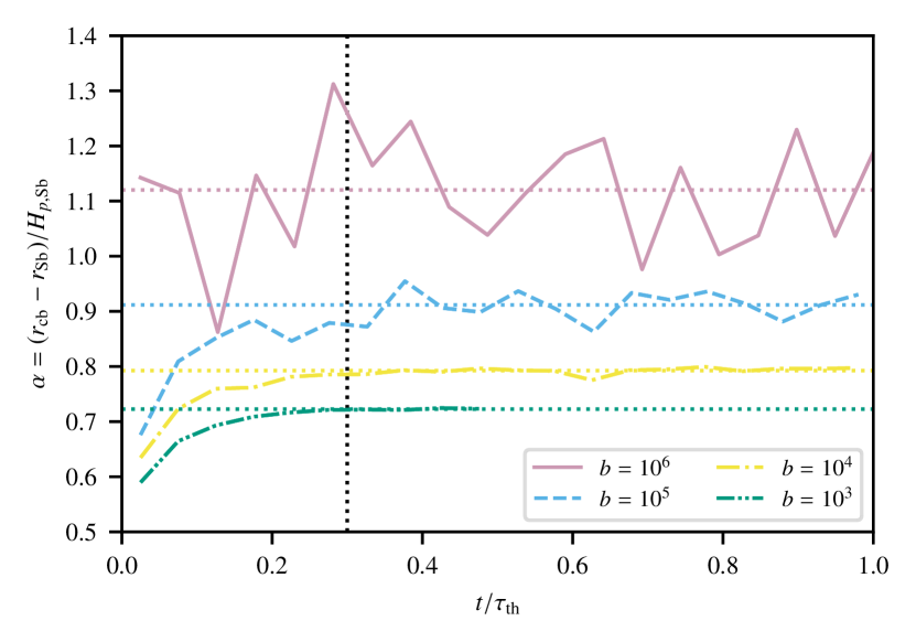
Figure 8: Time evolution of the dimensionless penetration distance $\alpha=(r_{\mathrm{cb}}-r_{\mathrm{Sb}})/H_{p,\mathrm{Sb}}$, where $r_{\mathrm{cb}}$ is the radius of the convective boundary, $r_{\mathrm{Sb}}$ the radius of the Schwarzschild boundary, and $H_{p,\mathrm{Sb}}$ the pressure scale height at $r_{\mathrm{Sb}}$. The four example simulations are 2.5D with $N_{r}=512$. The time axis shows the time as a fraction of the thermal time scale $\tau_{\mathrm{th}}(b)$. The dotted vertical line at $t=0.3\tau_{\mathrm{th}}$ marks the end of the initial transient. Each data point corresponds to a time average over $0.05\tau_{\mathrm{th}}$.

We show the radial profiles of the temperature gradient $\nabla$ in 2.5D simulations with four different boost factors in Fig. 9. The stratification in the core becomes increasingly closer to being adiabatic as the boost factor is decreased. However, the stratification is at least slightly sub-adiabatic at $r\gtrsim 0.17R_{\star}$, which is well inside the Schwarzschild boundary at all four boost factors. The drop in the temperature gradient at the convective boundary (the outer boundary of the penetration layer) becomes increasingly steep with decreasing boost factor.

Our simulations suggest that a simplified model, often referred to as ,,step overshoot”, which assumes that the penetration layer is fully mixed, perfectly adiabatic, and ends with a discontinuous jump to the radiative temperature gradient at the convective boundary is a good approximation to the thermal structure to be expected at the nominal luminosity ($b=1$). A MESA model of a $15$ M_⊙ ZAMS star computed using a parametric description of the penetration process is shown in Fig. 9 for comparison. We use $\alpha=0.6$ in this model, which is approximately the value we obtain by extrapolating the results of our 2.5D simulation to the actual stellar luminosity ($b=1$) in Sect. 3.5.

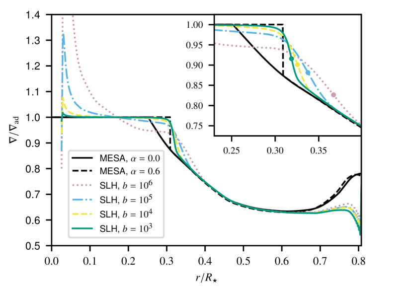
Figure 9: Radial profiles of the temperature gradient $\nabla$ in 2.5D simulations with $N_{r}=512$ and the boost factors given in the legend. The gradients are normalised using the adiabatic temperature gradient $\nabla_{\mathrm{ad}}$. The curves are derived from simulation data averaged over the time interval $0.3\tau_{\mathrm{th}}\leq t\leq\tau_{\mathrm{th}}$ except for the $b=10^{3}$ simulation, for which we use the interval $0.3\tau_{\mathrm{th}}\leq t\leq 0.5\tau_{\mathrm{th}}$. MESA models with $\alpha=0.0$ (our initial condition) and $\alpha=0.6$ are shown for comparison. The inset zooms in onto the convective-penetration layer with dots marking the location of the steepest gradient in $\nabla/\nabla_{\mathrm{ad}}$.

3.4 Numerical convergence of the penetration distance

For each boost factor and grid dimensionality, we run simulations on a range of grids in order to quantify and suppress discretisation effects. Figure 10 shows that 2.5D simulations with the highest boost factor ($b=10^{6}$) are consistent with having the same value of $\alpha$ for all of our 2.5D grids ($N_{r}=128$ to $N_{r}=1024$), i.e. the simulations resolve all relevant scales well enough and $\alpha$ is numerically converged. The remaining sets of 2.5D and 3D simulations show some resolution dependence. For our second-order code, we would asymptotically expect the dependence $\alpha=\alpha_{\infty}+CN_{r}^{-2}$, where $\alpha_{\infty}$ is the unknown value of $\alpha$ for $N_{r}\to\infty$, and the constant $C$ sets the magnitude of the error term. We observe first-order convergence, $\alpha=\alpha_{\infty}+CN_{r}^{-1}$, instead, see Fig. 10. Nevertheless, we can fit this law to the data to obtain the extrapolated penetration distance $\alpha_{\infty}$ that would correspond to a hypothetical, infinitely fine grid. We employ the Monte Carlo procedure described in Sect. 3.2, so we obtain a statistical-variation range in addition to the mean fit. We exclude the simulations with $N_{r}=128$ ($N_{r}^{-1}=7.8\times 10^{-3}$) for the two lowest boost factors because these simulations seem to be under-resolved and they deviate significantly from the fits based on finer grids. None of the points included in the fits deviate from the fitting lines by more than $2\sigma$. The resulting values of $\alpha_{\infty}$ are summarised in Table 2.

Table 2: Dimensionless penetration distance extrapolated to infinite grid resolution.

DIM	$b$	$\alpha_{\infty}$
2.5D	$10^{6}$	$1.124\pm 0.022$
2.5D	$10^{5}$	$0.944\pm 0.006$
2.5D	$10^{4}$	$0.862\pm 0.002$
2.5D	$10^{3}$	$0.781\pm 0.001$
3D	$10^{6}$	$1.090\pm 0.025$
3D	$10^{5}$	$0.718\pm 0.007$

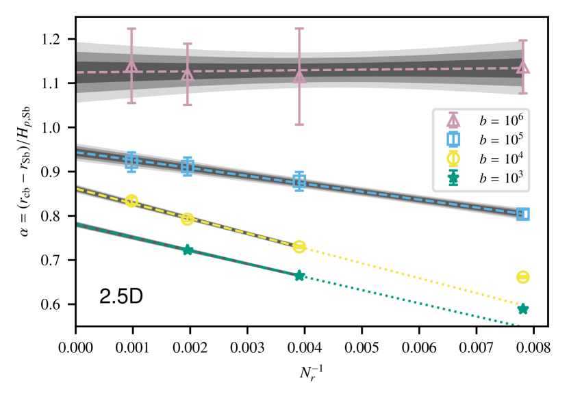
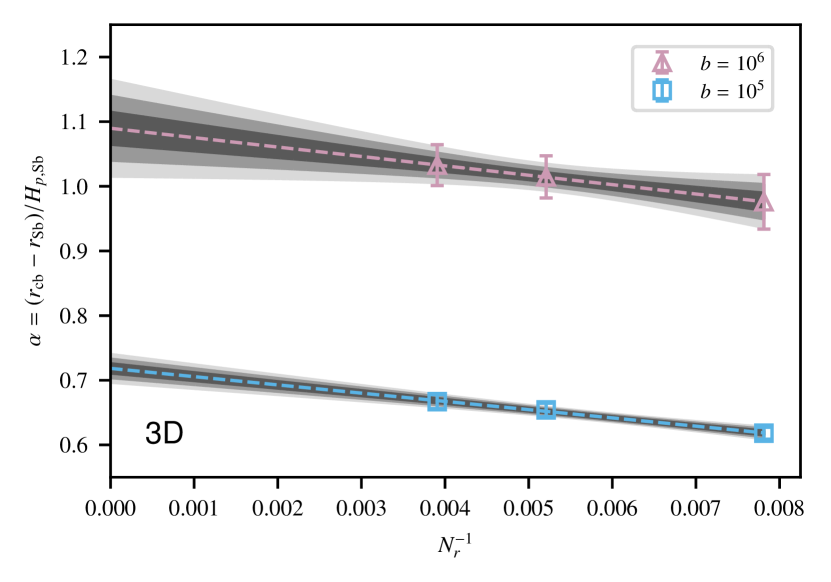
Figure 10: Numerical convergence of the penetration distance $\alpha$ for 2.5D and 3D simulations with different boost factors $b$. The radial grid spacing is expressed as the inverse number of radial grid cells, $N_{r}^{-1}$, so that first-order convergence corresponds to a straight line. The error bars indicate $3\sigma$ intervals of statistical variation. The grey shading shows $\sigma$, $2\sigma$, and $3\sigma$ statistical-variation intervals of the fits. The dashed lines show the mean fit in each case and the dotted lines extrapolate the fits towards data points excluded from the fitting procedure.

3.5 Luminosity dependence of the penetration distance

Having suppressed discretisation effects, we are left with a single estimate of the penetration distance and its range of statistical variation for each boost factor and grid dimensionality. We show these data points in Fig. 11. The 2.5D data points suggest a weak, although highly statistically significant, dependence of $\alpha$ on the boost factor $b$. We first blindly fit power laws to the 2.5D and 3D data sets individually using the Monte Carlo procedure described in Sect. 3.2. In the 2.5D case, the scaling exponent is only $0.043\pm 0.001$ and the penetration distance extrapolated to the nominal luminosity ($b=1$) is $\alpha_{2.5D}=0.580\pm 0.005$. If we assume that the $\alpha(b)$ dependence for 3D simulations can also be described by a single power law, we obtain a much steeper scaling with an exponent of $0.181\pm 0.011$. After extrapolating over five orders of magnitude, the power law would then imply a penetration distance of only $\alpha_{3D}=0.089\pm 0.012$. However, our current set of 3D simulations on its own does not contain enough evidence for the single-power-law model.

It is also possible that there is a power-law dependence $\alpha(b)$ but only for sufficiently low boost factors $b$, e.g. due to compressibility effects. Indeed, the 2.5D data point with $b=10^{6}$ deviates from the scaling law discussed above and shown in Fig. 11 by $3.2\sigma$. Therefore, we now exclude the $b=10^{6}$ data points and explore the alternative assumption that the power law’s slope is the same for 2.5D and 3D simulations with $b\leq 10^{5}$. Figure 12 shows that the scaling exponent based on the three remaining 2.5D data points remains essentially unchanged ($0.042\pm 0.001$) because the statistical weight of the $b=10^{6}$ data point considered in the fit in Fig. 11 is low. The largest deviation from the power law is only $0.5\sigma$ now. The penetration distance implied by the 2.5D simulations at the nominal luminosity does not change significantly either ($\alpha_{2.5D}=0.585\pm 0.005$). However, the much shallower scaling implies a much larger extrapolated penetration distance of $\alpha_{3D}=0.443\pm 0.006$ for the 3D simulations if we fix the scaling exponent and simply shift the 2.5D-based power law to make it pass through the 3D-based data point at $b=10^{5}$.

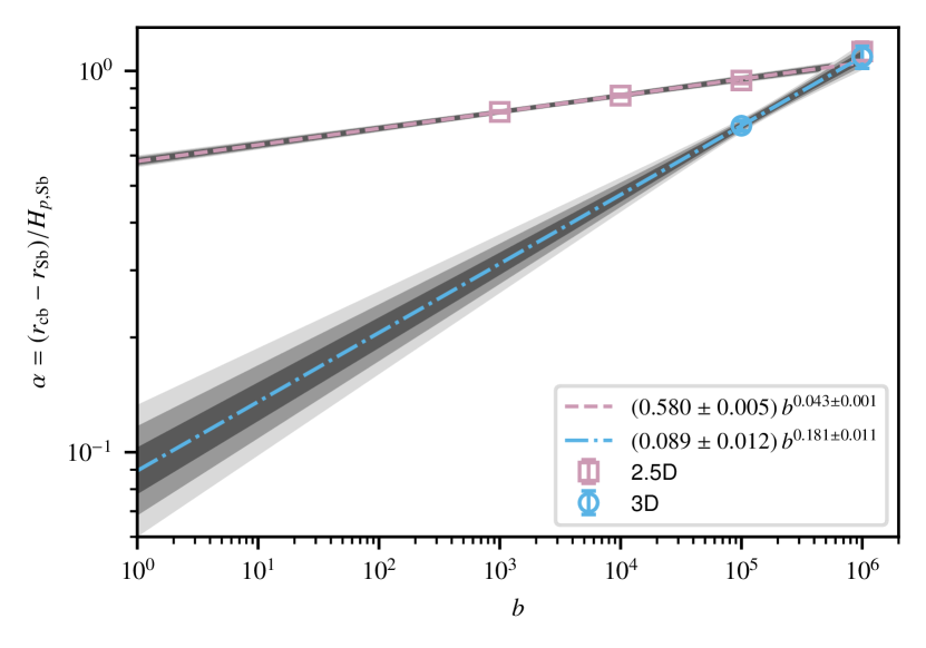
Figure 11: Penetration distance $\alpha$ extrapolated to an infinitely fine grid (see Fig. 10) as a function of the boost factor $b$. Assumed power-law dependencies $\alpha(b)$ are fitted to the 2.5D and 3D data points separately. The grey shading shows $\sigma$, $2\sigma$, and $3\sigma$ statistical-variation intervals of the fits.

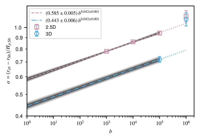
Figure 12: As Fig. 11 but here we exclude the simulations with $b=10^{6}$, fit a power law to the remaining 2.5D data points and, assuming that the scaling exponent is the same in 3D, we shift the power law to pass through the data point based on 3D simulations with $b=10^{5}$. The statistical variation associated with that data point is added to that associated with the scaling law.

4 Summary and discussion

Observational evidence strongly suggests that convective cores of intermediate-mass and massive, main-sequence stars are substantially larger that what is predicted by linear stability analysis. The process of convective penetration, first described by Roxburgh (1978), seems to be able to enlarge the convective cores of main-sequence stars enough to reconcile them with observations. However, the penetration distance depends on the complex physics of 3D turbulent convection in the core and such effects cannot be consistently captured in analytic treatments.

We have performed a large set of simulations of convective penetration in a chemically homogeneous model of a $15$ M_⊙ ZAMS star. We make it possible to cover the thermal time scale by increasing the luminosity and decreasing the opacity by the same large boost factor $b$ ranging from $10^{3}$ to $10^{6}$. This scaling procedure preserves the value of the radiative temperature gradient. We run both 2.5D and 3D simulations using our time-implicit, low-Mach-number code SLH and quantify their numerical convergence using a range of computational grids.

Comparing SLH simulations with and without radiative diffusion, we demonstrate that there is no process to stop mass entrainment into the core in the absence of radiative diffusion and the star becomes fully convective. Simulations with radiative diffusion reach a statistically stationary state with a convective core and radiative envelope on the thermal time scale.

All of our simulations with radiative diffusion show a clear penetration layer, the thickness of which becomes statistically constant in time once thermal equilibrium has been reached. As expected, simulations performed with large luminosity boost factors show large deviations from adiabacity in the core. However, the core, including the bulk of the penetration layer, becomes nearly adiabatic as the luminosity is decreased. This result qualitatively agrees with the simulations of penetrative convection in similar stellar environments performed by Baraffe et al. (2023), Mao et al. (2023), and Blouin et al. (2023) as well as with the much more idealised simulations of Anders et al. (2022).

There is a steep jump from the adiabatic to the radiative temperature gradient at the outer boundary of the penetration layer. This means that the popular simplified model, often referred to as „step overshoot”, which assumes that the penetration layer is fully mixed, perfectly adiabatic, and ends with a discontinuous jump to the radiative temperature gradient at the convective boundary, is a good approximation to the thermal structure to be expected at the nominal luminosity ($b=1$).

We find strong evidence for a weak dependence of the dimensionless penetration distance $\alpha$ on the boost factor $b$. Weak if any dependence of the core size on $b$ is expected also from the theoretical point of view. In the Roxburgh criterion (Eq. (1)), the energy flux $\overline{\Gamma}$ due to nuclear sources scales in proportion to $b$. So does the radiative flux $\overline{F}$ because we scale the opacity in inverse proportion to $b$. The turbulent dissipation rate $\Phi_{0}$ is expected to scale with $u_{\mathrm{conv}}^{3}/L_{\mathrm{turb}}$, where $L_{\mathrm{turb}}$ is an integral length scale of the turbulence. If $L_{\mathrm{turb}}$ is fixed and we consider adiabatic convection, we have the usual scaling $u^{3}\propto b$, so both sides of Eq. (1) scale in proportion to $b$ and the size of the core cannot depend on $b$. However, we show in Sect. 3.2 and Fig. 6 that the velocity scaling in our non-adiabatic simulations is slightly shallower than that of adiabatic convection. This changes the relative importance of the dissipation term as $b$ is varied over several orders of magnitude. The slight change in the core radius $r_{\mathrm{cb}}$ itself may affect the dissipation rate since it is reasonable to assume that $L_{\mathrm{turb}}\propto r_{\mathrm{cb}}$. We must also keep in mind that Roxburgh (1989) assumes the velocity vector to vanish at the convective boundary and that contributions from terms quadratic in fluctuations can be neglected. Some of those terms may not be negligible in our simulations, especially because some energy flux is needed to drive the waves we clearly see in the radiative envelope.

Extrapolating the results of our 2.5D simulations to $b=1$, we derive a rather large penetration distance $\alpha=0.585\pm 0.005$. Our set of 3D simulations covers only two relatively large boost factors at the moment. For this reason, we show two possible extrapolations to $b=1$ in Sect. 3.5, which give penetration distances $\alpha=0.089\pm 0.012$ and $\alpha=0.443\pm 0.006$. These two values differ by a factor of $5$ but both are broadly consistent with observations. For stars of similar masses, the compilation of Anders & Pedersen (2023, their Fig. 12) of observational constraints on the penetration distance from asteroseismology shows measurements and upper limits roughly spanning our two 3D-simulation-based $\alpha$ estimates. Brott et al. (2011) discuss a drop in rotational velocity observed at a certain value of surface gravity in a sample of stars in the Large Magellanic Cloud. Interpreting the drop as the terminal-age main sequence, their calibration gives $\alpha=0.34\pm 0.1$ for stellar models in the mass range approximately from $10$ to $20$ M_⊙. The calibration of Claret & Torres (2016), based on eclipsing binaries, shows that $\alpha$ increases from zero at $1.2$ M_⊙ to ${\approx}\,0.2$ at $2.1$ M_⊙, where it stops changing and remains approximately the same up to $4.4$ M_⊙. The fitting formula given by Eqs. (11) – (16) of Jermyn et al. (2022), which is based on the simulations and theory of Anders et al. (2022), gives $\alpha=0.19$ for a $15$ M_⊙ star.

The results presented here demonstrate only the most basic properties of the rich data set we have created. An analysis based on Reynolds averaging is already in progress and it is expected to quantify differences between our 2.5D and 3D simulations and become a basis for constructing simplified models of the penetration process. We are also working on extending our simulations, especially those in 3D geometry, to lower luminosity boost factors. Although the simulations are based on a realistic stellar model, the model is chemically homogeneous and it does not rotate or contain magnetic fields. Additionally, our computational grid currently covers a spherical wedge rather than the full sphere. All of these assumptions and simplifications should be gradually relaxed in order to generate predictions for a wide range of observed stars.