Local null controllability of a class of non-Newtonian incompressible viscous fluids
Abstract
We investigate the null controllability property of systems that mathematically describe the dynamics of some non-Newtonian incompressible viscous flows. The principal model we study was proposed by O. A. Ladyzhenskaya, although the techniques we develop here apply to other fluids having a shear-dependent viscosity. Taking advantage of the Pontryagin Minimum Principle, we utilize a bootstrapping argument to prove that sufficiently smooth controls to the forced linearized Stokes problem exist, as long as the initial data in turn has enough regularity. From there, we extend the result to the nonlinear problem. As a byproduct, we devise a quasi-Newton algorithm to compute the states and a control, which we prove to converge in an appropriate sense. We finish the work with some numerical experiments.
keywords:
Null controllability, shear dependent viscosity, nonlinear partial differential equations, non-Newtonian fluids.MSC:
[2010] 35K55, 76D55, 93B05, 93C10.1 Introduction
Let us fix an integer and let us take a non-empty, open, connected, and bounded subset of with a smooth boundary and a real number Henceforth, we write and In general, we understand all of the derivatives figuring in this work in the distributional sense.
We interpret the set as a region occupied by the particles of a fluid with a velocity field We represent its pressure by whereas stands for a distributed control which acts as a forcing term through a given open set We assume The model comprising the subject of the current investigation is the following:
| (1) |
Above, the function denotes the indicator function of we define the material derivative as
| (2) |
the stress tensor, is given by
| (3) |
in such a way that the constitutive law for the deviatoric stress tensor reads as
| (4) |
where
We remark that the three constants and appearing above are strictly positive, typically with although this assumption is not necessary in this work.
Therefore, we are focusing on the class of power-law shear-dependent fluids. Pioneers in the study of the system (1)-(4) were O. A. Ladyzhenskaya and J.-L. Lions, see [28, 27, 26, 31]. Particularly, let us introduce the usual spaces we use in the mathematical analysis of fluid dynamics, i.e.,
and
where denotes the outward unit normal on Then, the results [31, Chapitre 2, Thèoremes 5.1-5.2] (cf. [31, Chapitre 2, Remarque 5.4]) imply the following:
Theorem 1.
For and the system (1)-(4) is the simple turbulence model of Smagorinsky, see [46]. Since then, gradient-dependent (or shear-dependent) viscosity models of incompressible viscous fluids have attracted considerable attention from the mathematical, physical, and engineering communities. Some other works investigating the well-posedness for the model (1)-(4) under consideration are [40, 16, 33, 35, 34]. The paper [29] studies the energy dissipation for the Smagorinsky model. For the investigation of some regularity properties of solutions of (1)-(4), see [2] and the references therein.
On the one hand, the Navier-Stokes (NS) system of equations (corresponding to formally replacing in (4)) is deeply relevant, not only in mathematics, but for physics, engineering, and biology, see [50, 45]. For standard well-posedness results, which are now classic, see [51, 3]. However, even with a great effort of researchers, among the main longstanding open problems are the questions about global existence or finite-time blow-up of smooth solutions in dimension three of the incompressible Navier-Stokes (or else the Euler) equations. The system (1)-(4) is a generalization of the Navier-Stokes equations. From a practical perspective, as [16] points out, every fluid which solutions of NS decently models is at least as accurately described by those of (1)-(4).
On the other hand, for real-world problems, the advantage of considering the more general fluids of power-law type is not slight. In effect, as [35] describes, practitioners employed them to investigate problems in chemical engineering of colloids, suspensions, and polymeric fluids, see [49, 48, 52, 4, 9, 41, 44], in ice mechanics and glaciology, see [37, 53, 25], in blood-rheology, see [8, 7, 10, 14, 15, 39, 47, 17], and also in geology, see [36], to name a few instances.
We briefly describe the physical meanings of the constants and Firstly, stands for the kinematic viscosity of the fluid. If the physical variables are nondimensionalized, then is the Reynolds number of the fluid. Secondly, we can conceive the constants and in light of the kinetic theory of gases and the definition of a Stokesian fluid, see [26, 27]. For instance, from the point of view of turbulence modeling, we have where is a model parameter and is a mixing length, see [42]. In the latter perspective, a possible derivation of the model stands on the Boussinesq assumption for the Reynolds stress, further stipulating that the eddy viscosity takes the particular form
| (5) |
see [30, 43]. The term given by (5) leads to a stabilizing effect by increasing the viscosity for a corresponding increase in the velocity field gradient, see the discussion in [16]; hence, we call these fluids shear-thickening.
From the viewpoint of control theory, [19] establishes the local null controllability for the Navier-Stokes equations under no-slip boundary conditions; later developments worth mentioning are, e.g, [20, 11, 5, 12]. For the study of the Ladyzhenskaya-Smagorinsky model, see [21]. The paper [38] deals with a similar one-dimensional problem. Regarding local exact controllability properties for scalar equations having a locally nonlinear diffusion, some advances are [23, 6, 32]. However, although the diffusion coefficients can be functions of the state (in the case of [6] in a simplified form), the methods used in these works seem not enough to tackle the situation in which these coefficients depend on the gradient of the controlled solution. Furthermore, the assumptions they make rule out more general diffusions with power-law type nonlinearities. In the present work, we can circumvent all of these difficulties.
The notion of controllability we consider in this paper is defined as follows.
Definition 1.
We now state the main theoretical result we establish in this paper.
Remark 1.
Although we stated Theorem 1 in terms of weak solutions, our methodology yields smooth controls and transient trajectories for the nonlinear system (1)-(4). Namely, we will be able to prove that there is a control parameter such that
with a corresponding trajectory satisfying
for appropriate time-dependent positive weights which blow up exponentially as For more details and the proofs, we refer to Sections 2 and 3. Of course, there is a trade-off between such regularity and our requirements on the initial datum. We will comment upon questions that are related to this relation on Section 5.
We will prove Theorem 2 with the aid of a local inversion-to-the-right theorem. Namely, we will introduce Banach spaces and (we provide the details in the second subsection of Section 3) as well as a mapping such that a solution of the equation
| (7) |
for a given initial data meeting the assumptions of Theorem 2, is a solution of the control problem, i.e., a tuple subject to (1)-(4) and (6). We will use the inversion theorem to guarantee the existence of a local right inverse of For proving that is well-defined, as well as that it enjoys suitable regularity properties, the key steps are novel high-order weighted energy estimates for a control and the solution of the linearization of the system (1)-(4) around the zero trajectory.
Taking advantage of the invertibility properties of we construct the following algorithm allowing the computation of a tuple solving (1)-(4) and (6).
The following local convergence result for Algorithm 1 holds.
Theorem 3.
There exist a small enough constant as well as appropriate Banach spaces and 111We provide, in the second subsection of Section 3, the explicit definitions of both and such that, if with satisfying the compatibility conditions of Definition 1, then it is possible to find with the following property: the relations and
imply the existence of for which
for all In particular, in
Here, we fix some notations that we will use throughout the whole paper. Firstly, denotes a generic positive constant that may change from line to line within a sequence of estimates. In general, depends on and In case begins to depend on some additional quantity (or we want to emphasize some dependence), we write We will also write, for every integer
where we used the standard multi-index notation above. We denote the standard norm of by Finally, we set
We finish this introductory section outlining the structure of the remainder of the work.
-
1.
In Section 2, we study the linearization of (1)-(4) around the zero trajectory — it is a forced Stokes system. With the aid of a global Carleman estimate, we can to show that this system is null controllable. Assuming sufficiently regular initial data, we employ a bootstrapping argument to deduce higher regularity for the control, taking advantage of its characterization via Pontryagin’s minimum principle. The higher control regularity naturally leads to higher regularity of the velocity field..
- 2.
-
3.
It is in Section 4 that we prove Theorem 3. Then, we conduct some numerical experiments to illustrate our theoretical findings.
-
4.
Finally, we conclude the work in Section 5 with some comments and perspectives.
2 Study of the linearized problem
2.1 Some previous results
Our aim in the present Section is to establish the null controllability of the linear system:
| (8) |
In (8), we have written We achieve this result via a suitable Carleman inequality for the adjoint system of (8); upon writing it reads
| (9) |
In the present subsection, we fix notations that we will employ henceforth. Let us consider with For the proof of the following lemma, see [24].
Lemma 1.
There is a function satisfying
We take with
We define
and
Remark 2.
Given there exists such that for all
For we write
We are ready to recall the Carleman inequality that is the key to study the null controllability of the linear system (8).
Proposition 1.
There exist positive constants and depending solely on and for which the relations and imply
where is the solution of (9) corresponding to and .
As a consequence, we get the following Observability Inequality.
Corollary 1.
With the notations of Proposition 1 (possibly enlarging and the latter now depending on ), we have
From now on, we fix and Moreover, in view of Remark 2, given we can take large enough in such a way that
| (10) |
Whenever we need (10) in subsequent estimates, for a suitable positive real number we will assume it holds in all that follows.
For we introduce the weights
Regarding these weights, it is valuable to note:
Remark 3.
Let be nine real numbers.
-
(a)
One has the equality In particular, for integral
-
(b)
There exists a constant such that
-
(c)
There exists a constant such that if, and only if,
We define the weights
and
With these notations, we can gather Proposition 1 and Corollary 1 together, resulting in the following statement.
Corollary 2.
There is a constant such that the solution of (9) corresponding to and satisfies
2.2 Null controllability of the linear system
Theorem 4.
We suppose Then there exist controls such that the state of (8) corresponding to and satisfies
| (11) |
where
In particular, almost everywhere in
Proof.
We define we take with and we consider on the continuous bilinear form
By Corollary 2, is an inner product on Let us denote i.e., is the completion of under the norm induced by We also deduce, from the corollary we just mentioned, that that the linear form
is continuous, with
The Riesz representation theorem guarantees the existence of a unique for which
| (12) |
Upon taking above, we get
whence
Let us set
| (13) |
We observe that that is a solution of (8) corresponding to the datum and and applying Corollary 2 once more,
This proves the theorem. ∎
2.3 Weighted energy estimates
Along this subsection, we let and let us denote by the control-state pair constructed in the proof of Theorem 4.
Lemma 2.
Let us define and We have
| (14) |
and, if then
| (15) |
where
Proof.
For each let and be the projections of of and in the first eigenfunctions for the Stokes operator respectively. Let us denote by the corresponding solution for the finite dimensional approximate forced Stokes system. For simplicity, unless we state otherwise, we omit the subscript throughout the current proof. Moreover, we emphasize that we can take all of the constants appearing below to be independent of
Using as a test function in system (8), and doing some integrations by parts, we derive the identity
| (16) | ||||
From (10) and Remark 3, item (c), we have whence
| (17) |
and
| (18) |
From Remark 3, item (b), we have from where it follows that
| (19) |
Using (17), (18) and (19) in (16), and applying Gronwall’s inequality together with (11), we infer (14).
Now, we use as a test function in (8), from where we easily derive that
| (20) |
We observe that, for any
| (21) |
| (22) |
| (23) |
We take sufficiently small, in such a way that that the terms involving in (21) and (22) are absorbed by the left-hand side of (20). Also, from (23) and (14), the time integral of the third term in the right-hand side of (20) is bounded by Thus, it suffices to apply Gronwall’s Lemma to conclude (15) for the Galerkin approximates instead of the actual solution Employing standard limiting arguments, as we conclude that (15) does hold for the actual solution ∎
Lemma 3.
-
(a)
If then
with the estimate
-
(b)
Let us also assume that For we have the memberships
and the following inequality holds
Proof.
(a) For we notice that
Choosing and it follows that
Thus, and solve the Stokes equation
where
By standard regularity results for solutions of the Stokes system, we can infer the stated regularity for
(b) As in the previous item, for we derive
For the choice it is straightforward to check the inequalities
and
We can conclude by arguing similarly as in the first two memberships and corresponding estimates. The third ones are obtained doing the same analysis for the term ∎
Lemma 4.
Let us set and Supposing we have the following estimates:
| (24) |
If furthermore
| (25) |
where
and
Proof.
We establish the current estimates by following the same approach as in the proof of Lemma 2. Here, we begin by differentiating the system (8) with respect to time, and we use as a test function:
| (26) | ||||
We note that
hence,
| (27) |
| (28) |
so that by using (27) and (28) in (26), then integrating in time and applying of Gronwall’s lemma, it follows that
| (29) | ||||
It is simple to infer the subsequent estimate:
| (30) |
Next, we use as a test function in the system (8) differentiated with respect to time to deduce
| (31) |
We observe that
| (32) |
and for each
| (33) |
as well as
| (34) |
We fix a sufficiently small whence the second terms within the brackets in the right-hand sides of (33) and (34) are absorbed by the left-hand side of (31). Then, using (32) in (31), we infer
| (35) |
Employing Gronwall’s lemma in (35), we obtain
| (36) |
We easily establish, with the aid of item (a) of Lemma 3, that
whence
| (37) |
Lemma 5.
We write and Let us assume that and Then, the following estimate holds
| (40) |
If, furthermore, and then
| (41) |
where we have written
Proof.
Again, we proceed in the same framework as in the proof of Lemma 2. We begin by applying the Stokes operator on the equation of system (8), and then use as a test function:
| (42) |
We integrate (42) with respect to time, whence
| (43) |
We can now easily argue that, under suitable limiting arguments (having in view the compatibility conditions we required in the statement of the present lemma), Eq. (43) yields the corresponding estimate for the solution of (8). We observe that the relations and imply with
| (44) |
In the differential equation of system (8) differentiated once with respect to time, we use the test function
| (45) | ||||
For
| (46) |
| (47) |
| (48) |
and
| (49) |
Therefore, by taking sufficiently small, and using (46)-(49) in (45), we deduce
| (50) |
Next, we differentiate the equation of system (8) twice with respect to time and we use the test function
| (51) | ||||
We have
| (52) |
| (53) |
| (54) |
and
| (55) |
Using (52), (53) and (54) in (51), then integrating in time and using (55), we infer
| (56) |
Estimates (43), (44), (50) and (56) are enough to conclude (40).
Now, we use as a test function in the equation of system (8) twice differentiated in time, reaching
| (57) |
For
| (58) |
| (59) |
and we also notice that
| (60) |
We easily check that
| (61) |
As in the proof of (40), inequalities (58)-(61), we can infer from (57), through an adequate choice of a small positive and the aid of the previous estimates, the subsequent inequality
| (62) |
Estimate (62) is precisely (41); hence, we have finished the proof of the present result. ∎
3 Null controllability of the model (1)
3.1 Local right inversion theorem
It is possible to find a proof of the subsequent result in [1]. This is the inversion theorem that we will use to obtain our local null controllability result.
Theorem 5.
Let and be two Banach spaces, and be a continuous function, with We assume that there are three constants and a continuous linear mapping from onto with the following properties:
-
(i)
For all we have
-
(ii)
The constants and satisfy
-
(iii)
Whenever the inequality
holds.
Then, whenever the equation has a solution where
A typical way of verifying condition (iii) is through the remark presented below.
Remark 4.
Let and be two Banach spaces, and let us consider a continuous mapping with of class Then it has property for any positive subject to as long as we take as the continuity constant of at the origin of
3.2 The setup
Let us set
We define
| (63) |
We consider on the norm
| (64) |
where in (64) we have written Then, endowing the space with renders it a Banach space.
Now, we put
| (65) |
| (66) | ||||
and also consider the space of initial conditions
with the same topology as Then, we define
| (67) |
The space with the natural product topology is also a Banach space.
Finally, we define the mapping by
| (68) |
3.3 Three lemmas and the conclusion
Lemma 6.
The mapping is well-defined, and it is continuous.
Proof.
We write where
| (69) |
There is nothing to prove about since it is cleary linear and continuous. We will consider only the mapping in what follows.
We decompose where
By the definition of the norm of it follows promptly that
Next, we will prove that the quantity is finite.
CLAIM 1:
We notice that
In the case the term vanishes and thus is bounded by Otherwise, assuming we have
In the above equations, we used the continuous immersions: These are valid for see [18], and we will use them tacitly henceforth.
Now, we obtain the estimate for
Likewise, we show to be finite, since
CLAIM 2:
We begin with the pointwise estimate,
As in the previous claim, if then For the next estimate is valid:
Proceeding similarly, we prove the remaining inequalities:
This finishes the proof of the second claim.
CLAIM 3:
As before, we begin by considering the pointwise estimate:
Again, if then we need not consider since it vanishes. For
and
These inequalities confirm the third claim.
The remaining terms composing the norm of are norms of lower order derivatives of it, compared to the ones considered above, in adequate weighted spaces. Therefore, these terms are even easier to handle. A similar remark is also true for In addition, we can show the continuity of via estimates which are very similar to the ones that we carried out in the claims above; hence, we omit these computations. This ends the proof of the Lemma. ∎
Lemma 7.
The mapping is strictly differentiable at the origin of with derivative given by
| (70) |
In fact, is of class and, for each its derivative is given by
| (71) |
where we have written
Proof.
We will only prove the first claim, i.e., that is strictly differentiable at the origin with being onto There is no additional difficulty to prove the lemma in its full force.
We write as in (69) of Lemma 6. Again, it is only necessary to investigate since is linear and continuous, and therefore Given we note that
where
Let us take two positive real numbers, and and we suppose We must show that we can take such that
We assume, without loss of generality, that It is enough to show that
| (72) |
for a suitable To begin with, we observe that
If then whereas for we also have If we follow estimates similar to the ones we developed in Lemma 6, and make use of the immersions we described there, in such a way that
Next, for
Now, for every
Summing up, the computations we carried out above yield
We can treat the remaining terms composing the norm of likewise, as we argued in Lemma 6. Dealing with is even simpler, since it involves lower order derivatives of In this way, we deduce that
Thus, it suffices to take any positive in order to finish the proof. ∎
Lemma 8.
The linear operator is continuous and onto. Furthermore, there exists a constant such that
| (73) |
Proof.
The continuity of follows promptly from the definition of the norms of and As for the surjectiveness of this mapping, let us consider We take as the state-pressure-control tuple given by Theorem 4. By the estimates we proved in subsection 2.3, namely (11), (14), (15), (24), (25), (40), and (41), together with Lemma 3, the membership is valid. Moreover,
where the last equality holds by the choice of hence, is onto By the aforementioned estimates, (73) follows easily. This establishes the lemma. ∎
3.4 Proof of Theorem 2
According to Lemmas 6, 7 and 8, it is licit to apply Theorem 5. This result allows us to deduce the existence of such that, for each subject to
| (74) |
the equation
| (75) |
has a solution which satisfies
| (76) |
for a suitable constant which is independent of Explicitly, we can take where is given by Lemma 8 (cf. (73)), and where we select the positive constant such that satisfies condition (iii) of Theorem 5. Such a constant does in fact exist by Lemma 7.
4 Numerical analysis
4.1 Proof of the convergence of the algorithm
The proof of this result is straightforward once we have established Lemmas 7 and 8. We present it here for completeness.
Firstly, we observe that Lemma 8 ensures that is well-defined in terms of since in this lemma we showed that is bijective. Furthermore, we have according to the notations of this lemma.
Next, we take with and we let be the solution of We also consider By Lemma 7, there exists such that the relations
imply
Shrinking if necessary, we can assume Employing Lemma 7 once more, we find such that and together imply
We write and let us assume By the algorithm,
whence
| (78) | ||||
Assuming inductively that which holds true for it follows that
| (79) |
Thus, we also have By induction, it follows that for every hence, it is always possible to pass from (78) to (79). Let us take Applying inequality (79) iteratively in we conclude that
This proves Theorem 3.
4.2 Implementation of the algorithm
To implement the fixed-point numerical algorithm, we proceed in two steps. Firstly, it is necessary to implement a solver for the control problem of the forced Stokes system. We begin with the variational problem (12) and adequately reformulate it to achieve a mixed formulation, as in [22, 21]. Below, we recall the main ideas for After treating the linear problem, we iterate it by updating the source term according to our algorithm.
Under the notations of the proof of Theorem 4 (see (13)), we define and Let us introduce the spaces
and
as well as the bilinear forms by
and
The last element we introduce is the linear form which is given by
We reformulate problem (12) as: find and multipliers such that
After we solve it, we recover the control and corresponding velocity field of the linear control problem (12) via
If we assume that is polygonal, it is simple to find finite dimensional approximations and of the spaces and
4.3 A numerical experiment
In the sequel, we will employ the FreeFem++ library of C++; see http://www.freefem.org/ff++ for more informations. In Table 1, we describe the datum we used to apply the quasi-Newton method for (1).
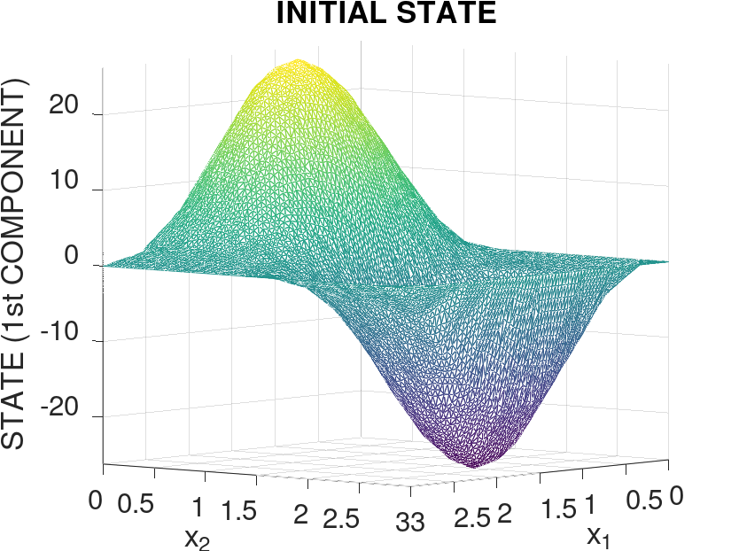
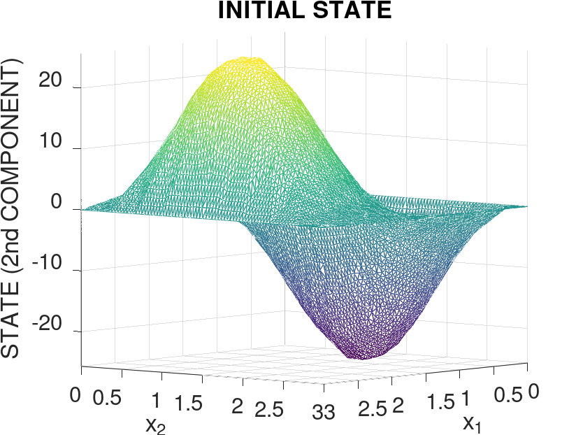
We illustrate in Figure 1 the mesh of and the mesh of the cylinder In Figure 2, we show both components of the initial state


Our stopping criterion is
with We took as the initial guess We attained convergence after six iterates, with a rate of .
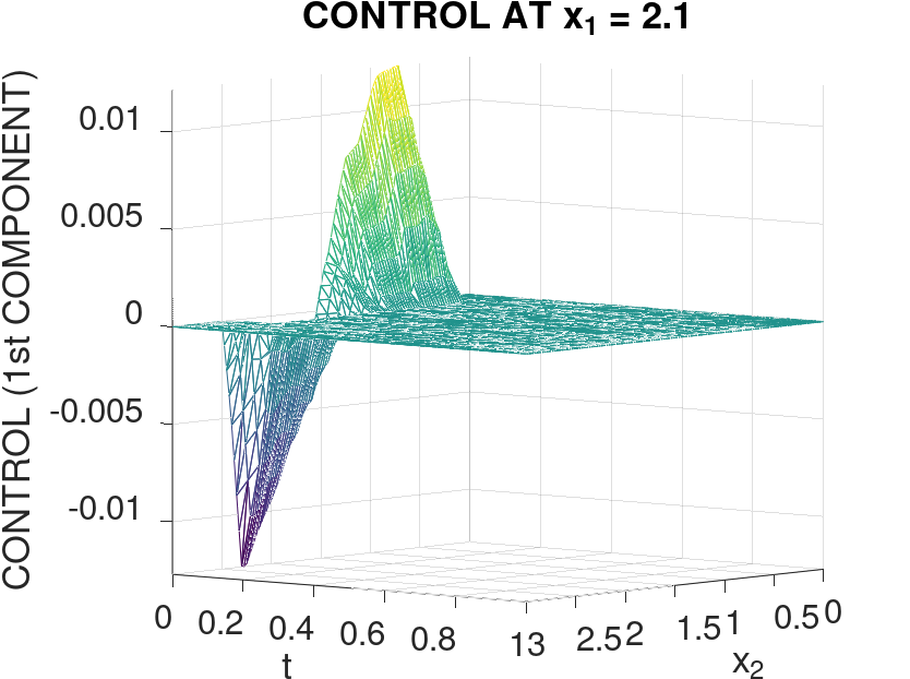
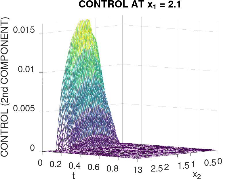
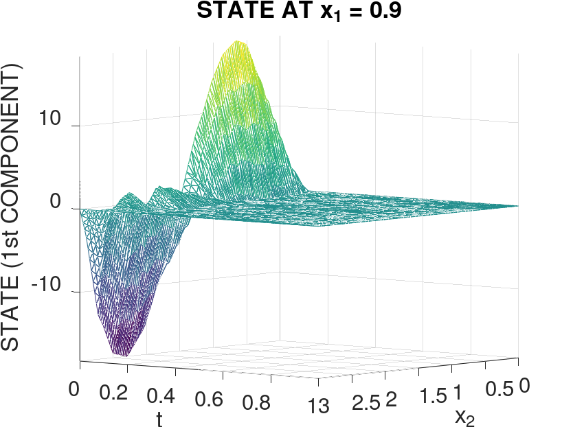
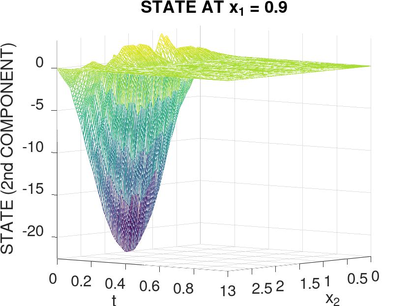
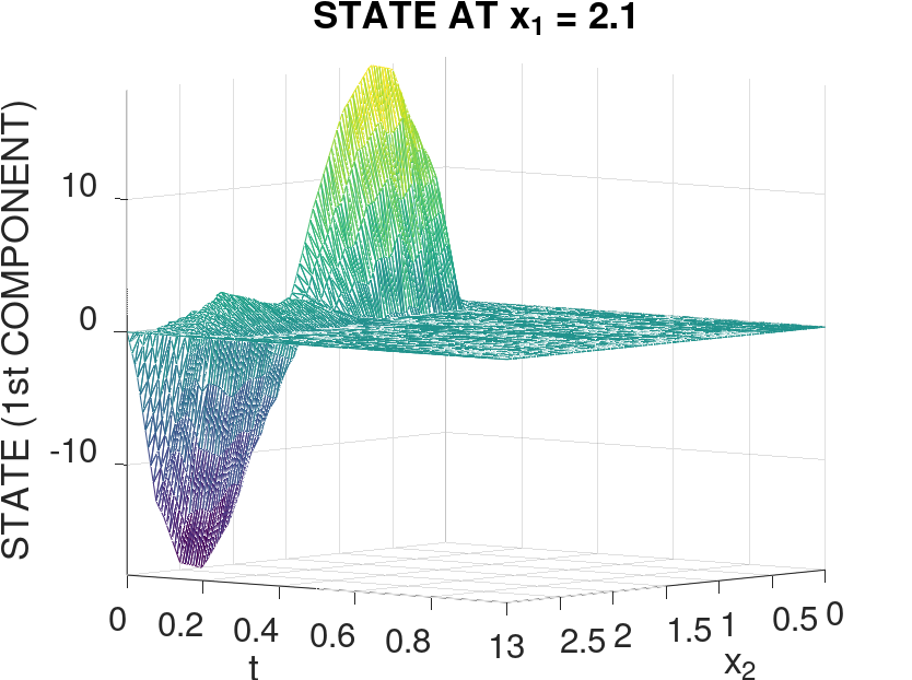
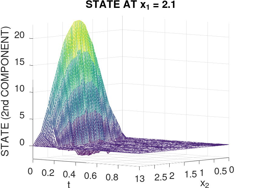
We begin to illustrate the overall behavior of the control and of the state we computed through the plots of some cross-sections in space of them. On the one hand, for the control, we plot the and cuts in Figures 3 and 4, respectively. On the other hand, we provide the surfaces comprising the values of the state components, relative to these cuts, in Figures 5 and 6.


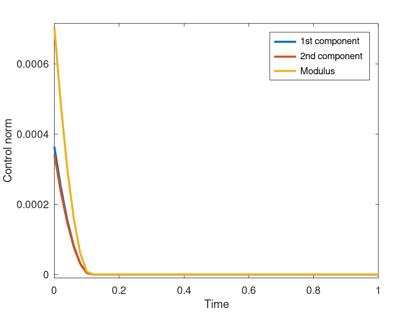
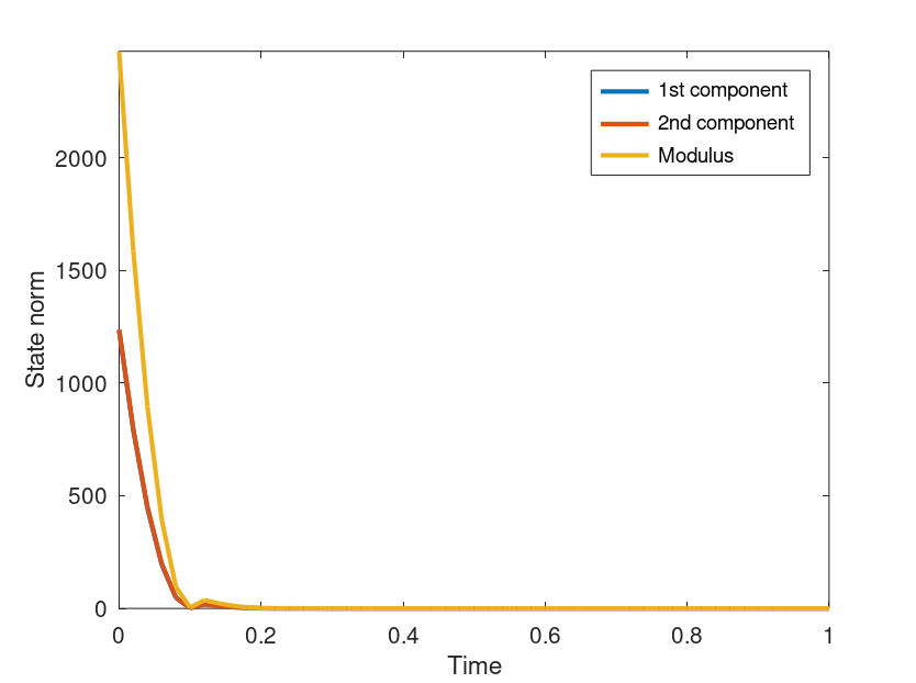
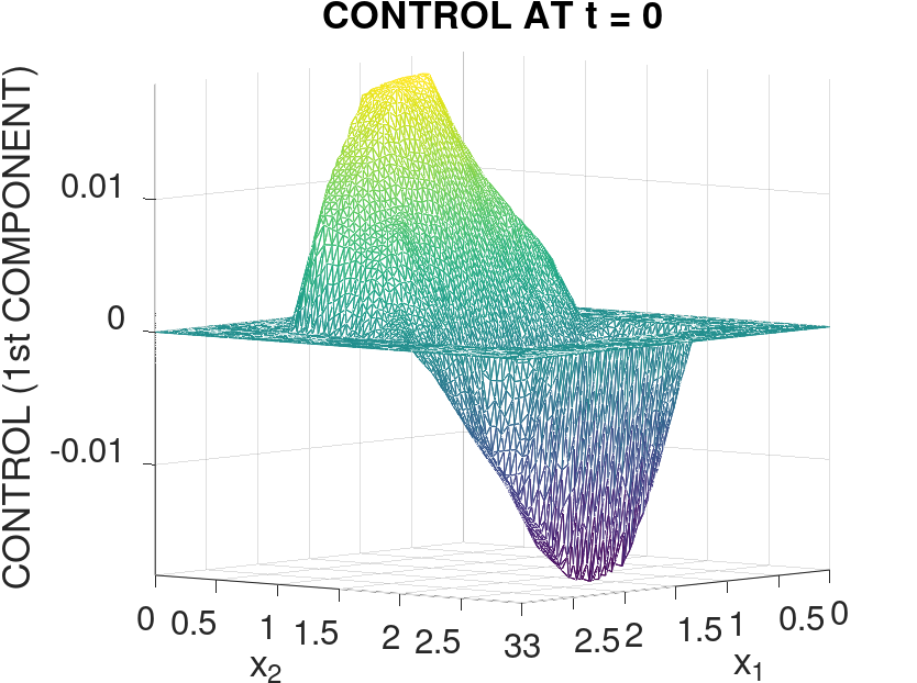
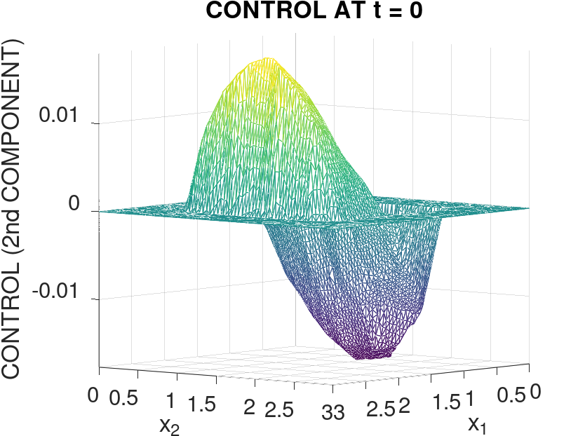
The time evolution of the norms of the control and of the corresponding state is what we illustrate in Figure 7. It corroborates our theoretical findings as these norms decay exponentially. To further illustrate the control, we provide a surface of its values at initial time in Figure 8. Then, we give some insight into the dynamics of the problem by showcasing some heat maps of the control and of its corresponding state. Namely, in Figure 9, we illustrate the control at time — it is already considerably small, as we would expect from Figure 7. For several times, viz., for each we give a heat map of the first (respectively, second) component of the velocity field in Figure 10 (respectively, Figure 11).


5 Comments and perspectives
5.1 On the constitutive law for the shear stress
Upon scrutinizing the proof of Lemmas 6 and 7, we conclude that they still hold for any function in (3) having the following properties:
-
1.
for some constant
-
2.
is of class
-
3.
There exists such that
for and for every
With Lemmas 6 and 7 at hand, we can follow the remaining steps towards the main result, i.e., Theorem 2, in the same manner as we proceeded in Section 3. This more general class of constitutive laws includes the one determining the reference model of this paper, namely, when or An example of another class of functions for which the properties we stated above hold are
5.2 On the use of the gradient instead of the deformation tensor
We can replace the gradient of the velocity field in (3) with the deformation tensor, without losing any of the results we established. From a practical viewpoint, this form of the model is more realistic. Analyzing the estimates we carried out throughout the present work, it is easy to see that the techniques we employed work just as well under this substitution. In particular, we notice the new framework shares the linearization around the zero trajectory with the one we studied in Section 2. Using the estimates developed there, alongside Korn-type inequalities, we can prove all of the corresponding results in Sections 3 and 4 for this alternate version of the model (1)-(4).
5.3 On extensions of Theorem 2 and some related open questions
Boundary controllability. We remark that a corresponding boundary local null controllability result follows from Theorem 2. In effect, let us assume that the initial data belongs to being sufficiently small in the (strong) topology of this space, and that we act with a control on a smooth portion of the boundary (with and ). We can employ standard geometrical arguments to extend to an open region with a smooth boundary and in a way that Acting distributively over with extended to zero outside of we obtain a control driving the corresponding state to zero at time A boundary control for the original problem is
Local controllability to trajectories. Regarding the local exact controllability to trajectories, there are two key aspects to investigate. Firstly, we must prove a global Carleman inequality, analogous to Proposition 1, but for the adjoint system of the linearization around the given trajectory, cf. Lemma 7. Secondly, we have to extend the estimates of Section 2 for this linearized problem. These endeavors are not straightforward, whence we leave this question open for future investigations.
On the restrictions on the exponent We notice that the estimates of Section 3 are not immediately extensible for the values of outside of However, we conjecture that our main result (viz., Theorem 2) is still in force for these values of A possible way to establish this is to parametrically regularize the function around zero, and attentively keep track of the regularization parameters throughout the estimates. We leave this question open here.
Requirements on the initial datum. Through another regularization argument, we possibly could require a less restrictive topology for the initial datum in the main theorem. Namely, if we assume only, we ought to carry out estimates for the uncontrolled problem (corresponding to (1) with ) to show that there exists for which as long as is sufficiently small. We choose not to delve in the technicalities of these estimates here (see [13, Lemma 5] for the application of such an argument in the case of the Navier-Stokes equations with the Navier boundary condition). However, we emphasize that this is a non-trivial task. Thus, assuming this is valid, Theorem 2 asserts that there exists a control driving to zero at time From the exponential decay of solutions, see [35, Theorem 4.5], this argument immediately provides a large-time global null controllability result.
Remarks on other boundary conditions. We observe that, if instead of no-slip boundary conditions, we assume Navier boundary conditions, the method of [13], used for the Navier-Stokes equations, may apply to the current model. If we manage to deal with the additional terms figuring in the expansions we must make after an appropriate time rescaling, especially the boundary layers, we should obtain a small-time global exact controllability to trajectories result (under Navier boundary conditions). Alternatively, if we consider the model (1)-(4) with (the dimensional torus) and periodic boundary conditions, then we can easily conduct the regularizing argument for the initial datum we outlined above, whence we can prove large-time global null controllability for this model — we omit the details here.
Stabilization results. It might be that, for an appropriate use of the stabilizing effect of the power-law model makes it easier to establish stabilization results for this class of non-Newtonian fluids. In this way, we propose that our current contributions could bridge such results with global null controllability ones. We remark that, even for the Navier-Stokes equations (corresponding to ) under no-slip boundary conditions, whether global null controllability holds is an open problem. We suggest that such results for (1)-(4) (with ) could provide insight on this important open question.
References
- Alekseev et al., [1987] Alekseev, V., Tikhomirov, V., and Fomin, S. (1987). Optimal Control. Springer Science & Business Media.
- Beirão da Veiga, [2005] Beirão da Veiga, H. (2005). On the regularity of flows with ladyzhenskaya shear-dependent viscosity and slip or non-slip boundary conditions. Communications on Pure and Applied Mathematics: A Journal Issued by the Courant Institute of Mathematical Sciences, 58(4):552–577.
- Boyer and Fabrie, [2012] Boyer, F. and Fabrie, P. (2012). Mathematical Tools for the Study of the Incompressible Navier-Stokes Equations andRelated Models, volume 183. Springer Science & Business Media.
- Carreau, [1968] Carreau, P. (1968). Rheological equations of state from molecular network theories. PhD thesis, PhD thesis, University of Wisconsin, Madison.
- Carreno and Guerrero, [2013] Carreno, N. and Guerrero, S. (2013). Local null controllability of the n-dimensional navier–stokes system with n- 1 scalar controls in an arbitrary control domain. Journal of Mathematical Fluid Mechanics, 15(1):139–153.
- Chaves-Silva and Guerrero, [2015] Chaves-Silva, F. W. and Guerrero, S. (2015). A uniform controllability result for the keller–segel system. Asymptotic Analysis, 92(3-4):313–338.
- Cho and Kensey, [1989] Cho, Y. and Kensey, K. (1989). Effects of the non-Newtonian viscosity of blood on hemodynamics of diiseased arterial flows, volume 1. Prat.
- Cho and Kensey, [1991] Cho, Y. I. and Kensey, K. R. (1991). Effects of the non-newtonian viscosity of blood on flows in a diseased arterial vessel. part 1: Steady flows. Biorheology, 28(3-4):241–262.
- Christiansen and Kelsey, [1973] Christiansen, E. and Kelsey, S. (1973). Isothermal and nonisothermal, laminar, inelastic, non-newtonian tube-entrance flow following a contraction. Chemical Engineering Science, 28(4):1099–1113.
- Cokelet et al., [1963] Cokelet, G. R., Merrill, E., Gilliland, E., Shin, H., Britten, A., and Wells Jr, R. (1963). The rheology of human blood—measurement near and at zero shear rate. Transactions of the Society of Rheology, 7(1):303–317.
- Coron and Guerrero, [2009] Coron, J.-M. and Guerrero, S. (2009). Null controllability of the n-dimensional stokes system with n- 1 scalar controls. Journal of Differential Equations, 246(7):2908–2921.
- Coron and Lissy, [2014] Coron, J.-M. and Lissy, P. (2014). Local null controllability of the three-dimensional navier–stokes system with a distributed control having two vanishing components. Inventiones mathematicae, 198(3):833–880.
- Coron et al., [2016] Coron, J.-M., Marbach, F., and Sueur, F. (2016). Small-time global exact controllability of the navier-stokes equation with navier slip-with-friction boundary conditions. arXiv preprint arXiv:1612.08087.
- Cross, [1965] Cross, M. M. (1965). Rheology of non-newtonian fluids: a new flow equation for pseudoplastic systems. Journal of colloid science, 20(5):417–437.
- Davies et al., [1990] Davies, P., Mazher, A., Giddens, D., Zarins, C., and Glagov, S. (1990). Effects of nonnewtonian fluid behavior on wall shear in a separated flow region. In Proc. 1st World Conf. of Biomech, volume 1, page 301.
- Du and Gunzburger, [1991] Du, Q. and Gunzburger, M. D. (1991). Analysis of a ladyzhenskaya model for incompressible viscous flow. Journal of Mathematical Analysis and Applications, 155(1):21–45.
- el Gibaly et al., [2016] el Gibaly, A., El-Bassiouny, O. A., Diaa, O., Shehata, A. I., Hassan, T., and Saqr, K. M. (2016). Effects of non-newtonian viscosity on the hemodynamics of cerebral aneurysms. In Applied Mechanics and Materials, volume 819, pages 366–370. Trans Tech Publ.
- Evans, [2010] Evans, L. C. (2010). Partial differential equations. American Mathematical Society, Providence, R.I.
- Fernández-Cara et al., [2004] Fernández-Cara, E., Guerrero, S., Imanuvilov, O. Y., and Puel, J.-P. (2004). Local exact controllability of the navier–stokes system. Journal de mathématiques pures et appliquées, 83(12):1501–1542.
- Fernández-Cara et al., [2006] Fernández-Cara, E., Guerrero, S., Imanuvilov, O. Y., and Puel, J.-P. (2006). Some controllability results forthe n-dimensional navier–stokes and boussinesq systems with n-1 scalar controls. SIAM journal on control and optimization, 45(1):146–173.
- Fernández-Cara et al., [2015] Fernández-Cara, E., Limaco, J., and de Menezes, S. (2015). Theoretical and numerical local null controllability of a ladyzhenskaya–smagorinsky model of turbulence. Journal of Mathematical Fluid Mechanics, 17(4):669–698.
- [22] Fernández-Cara, E., Münch, A., and Souza, D. A. (2017a). On the numerical controllability of the two-dimensional heat, stokes and navier–stokes equations. Journal of Scientific Computing, 70(2):819–858.
- [23] Fernández-Cara, E., Nina-Huamán, D., Nuñez-Chávez, M. R., and Vieira, F. B. (2017b). On the theoretical and numerical control of a one-dimensional nonlinear parabolic partial differential equation. Journal of Optimization Theory and Applications, 175(3):652–682.
- Fursikov and Imanuvilov, [1996] Fursikov, A. V. and Imanuvilov, O. Y. (1996). Controllability of evolution equations. Number 34. Seoul National University.
- Kjartanson et al., [1988] Kjartanson, B., Shields, D., Domaschuk, L., and Man, C.-S. (1988). The creep of ice measured with the pressuremeter. Canadian Geotechnical Journal, 25(2):250–261.
- [26] Ladyzhenskaya, O. (1970a). Modification of the navier–stokes equations for large velocity gradients. In Seminars in Mathematics VA Stheklov Mathematical Institute, volume 7.
- [27] Ladyzhenskaya, O. (1970b). New equations for the description of the viscoue incompressible fluids and solvability in the large of the boundary value problems for them. Boundary Value Problem of Mathematical Physics V, Amer. Math. Soc.: Providence.
- Ladyzhenskaya, [1969] Ladyzhenskaya, O. A. (1969). The mathematical theory of viscous incompressible flow, volume 2. Gordon and Breach New York.
- Layton, [2016] Layton, W. (2016). Energy dissipation in the smagorinsky model of turbulence. Applied Mathematics Letters, 59:56–59.
- Lesieur, [1987] Lesieur, M. (1987). Turbulence in fluids: stochastic and numerical modelling. Nijhoff Boston, MA.
- Lions, [1969] Lions, J. L. (1969). Quelques méthodes de résolution des problemes aux limites non linéaires.
- Liu and Zhang, [2012] Liu, X. and Zhang, X. (2012). Local controllability of multidimensional quasi-linear parabolic equations. SIAM Journal on Control and Optimization, 50(4):2046–2064.
- Málek et al., [1993] Málek, J., Nečas, J., and Rŭžička, M. (1993). On the non-newtonian incompressible fluids. Mathematical models and methods in applied sciences, 3(01):35–63.
- Málek et al., [2001] Málek, J., Necas, J., Ruzicka, M., et al. (2001). On weak solutions to a class of non-newtonian incompressible fluids in bounded three-dimensional domains: The case . Advances in Differential Equations, 6(3):257–302.
- Málek et al., [1995] Málek, J., Rajagopal, K. R., and Rŭžička, M. (1995). Existence and regularity of solutions and the stability of the rest state for fluids with shear dependent viscosity. Mathematical Models and Methods in Applied Sciences, 5(06):789–812.
- Malevsky and Yuen, [1992] Malevsky, A. V. and Yuen, D. A. (1992). Strongly chaotic non-newtonian mantle convection. Geophysical & Astrophysical Fluid Dynamics, 65(1-4):149–171.
- Metzner, [1956] Metzner, A. (1956). Non-newtonian technology: fluid mechanics, mixing, and heat transfer. In Advances in chemical engineering, volume 1, pages 77–153. Elsevier.
- Micu and Takahashi, [2018] Micu, S. and Takahashi, T. (2018). Local controllability to stationary trajectories of a burgers equation with nonlocal viscosity. Journal of Differential Equations, 264(5):3664–3703.
- Nakamura and Sawada, [1988] Nakamura, M. and Sawada, T. (1988). Numerical study on the flow of a non-newtonian fluid through an axisymmetric stenosis. Journal of Biomechanical Engineering, 110:137–143.
- Pokornỳ, [1996] Pokornỳ, M. (1996). Cauchy problem for the non-newtonian viscous incompressible fluid. Applications of Mathematics, 41(3):169–201.
- Powell and Eyring, [1944] Powell, R. E. and Eyring, H. (1944). Mechanisms for the relaxation theory of viscosity. Nature, 154(3909):427–428.
- Prandtl, [1952] Prandtl, L. (1952). Guide à travers la mécanique des fluides.
- Rebollo and Lewandowski, [2014] Rebollo, T. C. and Lewandowski, R. (2014). Mathematical and numerical foundations of turbulence models and applications. Springer.
- Ree et al., [1958] Ree, F., Ree, T., and Eyring, H. (1958). Relaxation theory of transport problems in condensed systems. Industrial & Engineering Chemistry, 50(7):1036–1040.
- Ruzicka, [2000] Ruzicka, M. (2000). Electrorheological fluids: modeling and mathematical theory. Springer Science & Business Media.
- Smagorinsky, [1963] Smagorinsky, J. (1963). General circulation experiments with the primitive equations: I. the basic experiment. Monthly weather review, 91(3):99–164.
- Steffan et al., [1990] Steffan, H., Brandstätter, W., Bachler, G., and Pucher, R. (1990). Comparison of newtonian and non-newtonian blood flow in stenotic vessels using numerical simulation. In Biofluid Mechanics, pages 479–485. Springer.
- Sutterby, [1966] Sutterby, J. (1966). Laminar converging flow of dilute polymer solutions in conical sections: Part i. viscosity data, new viscosity model, tube flow solution. AIChE Journal, 12(1):63–68.
- Sutterby, [1965] Sutterby, J. L. (1965). Laminar converging flow of dilute polymer solutions in conical sections. ii. Transactions of the Society of Rheology, 9(2):227–241.
- Tartar, [2006] Tartar, L. (2006). An introduction to Navier-Stokes equation and oceanography, volume 1. Springer.
- Temam and Chorin, [1978] Temam, R. and Chorin, A. (1978). Navier Stokes equations: Theory and numerical analysis. American Society of Mechanical Engineers Digital Collection.
- Turian, [1969] Turian, R. M. (1969). The critical stress in frictionally heated non-newtonian plane couette flow. Chemical Engineering Science, 24(10):1581–1587.
- Van Der Veen and Whillans, [1990] Van Der Veen, C. and Whillans, I. (1990). New and improved determinations of the velocity of ice stream-b and ice stream-c. West Antartica J. Glaciology, 36:324–339.