Coupled Quintessence scalar field model in light of observational datasets

Abstract

We do a detailed analysis of a well-theoretically motivated interacting dark energy scalar field model with a time-varying interaction term. Using current cosmological datasets from CMB, BAO, Type Ia Supernova, $H(z)$ measurements from cosmic chronometers, angular diameter measurements from Megamasers, growth measurements, and local SH0ES measurements, we found that dark energy component may act differently than a cosmological constant at early times. The observational data also does not disfavor a small interaction between dark energy and dark matter at late times. When using all these datasets in combination, our value of $H_{0}$ agrees well with SH0ES results but in 3.5$\sigma$ tension with Planck results. We also did AIC and BIC analysis, and we found that the cosmological data prefer coupled quintessence model over $\Lambda$CDM, although the chi-square per number of degrees of freedom test prefers the latter.

1 Introduction

The significant observational evidence about Universe’s dynamics [1, 2, 3] hint at the accelerated expansion at present. The elementary candidate to reveal the nature of this new physics includes Einstein’s cosmological constant $`\Lambda$’ with the equation of state (EoS) $`\omega$’ = $-1$ in the $\Lambda$CDM model. Though this model provides a good fit to the latest observations, it lacks solutions to other significant problems [4] in cosmology, especially to the fine-tuning problem and cosmic coincidence problem, also known as famous Why now? problem. Along with this, we still have no information about the nature of Dark Energy and Dark Matter. All we know is that our universe is composed of two types of perfect fluids, one of which is baryonic and responsible for the deceleration of the universe and the growth of structures. The other one, dominant at late times, has negative pressure and is responsible for the acceleration of the present universe. Both the components have different equation of state parameter $\omega=P/\rho$. The baryonic component is known to be like radiation-dominated, stiff matter, or the dust-like universe. However, the determination of the equation of state for dark energy ($\omega_{DE}$) is still one of the important unresolved questions in cosmology. Recent studies [5, 6, 7, 8, 9] rules out the possibility of $\omega_{DE}<<-1$ and other studies, SDSS and WMAP, [10] and [11] put bounds as $-$1.67 < $\omega_{DE}$ < $-$0.62 and $-$1.33 < $\omega_{DE}$ < $-$0.79 at present respectively.

Very recent results [12] and [13] very clearly rule out the possibility of rigid $\Lambda$ by $5\sigma$. In a complete cosmology model-independent way, the authors [14] showed at present, the universe requires a phantom equation of state ($\omega_{DE}<-1$) to explain the present observational datasets.

Thus, probing the cosmologists to explore beyond the standard model for dark energy candidates, perhaps dynamical dark energy model with varying EoS ($\omega$), see [15, 16, 17, 18], and references therein. The simplest possibility consists of a light scalar field such as a quintessence field, varying slowly during the Hubble time and can drive the accelerated expansion [19, 20, 21, 22, 23, 24]. Some studies also argue that the quintessence scalar field should couple (non-gravitationally) with the matter as provided by [25] unless some special symmetry inhibits the coupling. Such a coupling or interaction between Dark Energy (DE)/quintessence scalar field and Dark Matter (DM) can be characterized by a continuous energy flow or momenta between the two components. Many studies in the literature prescribe a purely phenomenological approach to deal with interacting cosmologies of dark sectors. Then, other classes of models are motivated from a field theory perspective and are well motivated. Numerous observations [26, 27, 28, 29, 30, 31, 32, 33, 34, 35, 36, 37] are in support of the theory of dark sector interaction, constraining energy transfer from DM to DE or the opposite paved their way into existence. Cosmological observations indicate that the coupling impacts the universe’s evolution [38, 39]. Effects of interaction on the CMB and linear matter power spectrum [40, 41] (for detailed review [42]), the structure formation at different scales and times and halo mass function [43, 44, 45, 46, 47] and on the behavior of the cosmological parameters [48, 49, 50] have been investigated in respective works. Based on these, coupled quintessence models were also studied theoretically in several other contexts [51, 52, 53, 54, 55, 56] to provide a viable cosmological solution. Interacting Dark Energy Models have also been studied extensively to alleviate "Hubble Tension" - which is now confirmed to be more than 5$\sigma$ after SH0ES 2022 results [57, 58, 59, 13]. Along with Hubble Tension is coupled the $S_{8}$ tension or $r_{drag}$ tension, i.e., the sound horizon at the drag epoch tension because BAO and CMB measure the product of $H_{0}$ and $r_{drag}$ and not $r_{drag}$ alone[60, 61]. Several works [62, 34, 63, 64, 65, 66, 67, 68, 69, 70, 42] tried to address these tensions in cosmology but could only solve one tension or the other by keeping the same number of parameters. The only solutions [71, 72, 64, 73, 74, 75] to resolve all cosmological tensions at present are those which are extremely fine-tuned or have more parameters and therefore increasing the uncertainties in the parameter space.

In the present work, we do a detailed and elaborate study of late-time cosmological dynamics. We mainly study the well-motivated dark matter and dark energy interaction case theoretically and try to understand how current observational data sets like CMB, Type Ia Supernovae, cosmic chronometers, BAO, Masers, growth rate data, and local $H_{0}$ measurement from SH0ES study influences the constraints on different cosmological parameters.

The work is structured as follows. In the next section, we present the model framework for the coupled dark sector and discuss its dynamics in brief. Later, we work out the linear dark matter perturbation evolution equation in section 3. Section 4 describes the observational data and methodology adopted in this work. Section 5 presents the results and thorough discussion from the observational analysis. We conclude the findings in Section 6.

2 Coupled field model and the Background dynamics

In our study, we assume that the geometry of the universe describing flat, isotropic, and homogeneous universe is given by Friedmann-Lema$\hat{i}$tre-Robertson-Walker (FLRW) metric and the line element for it is given by

$$\text{d}s^{2}=-\text{d}t^{2}+a^{2}(t)\big{(}\text{d}x^{2}+\text{d}y^{2}+\text{d}z^{2}\big{)}.$$ (2.1)

which when transformed into spherical coordinates reads as

$$\text{d}s^{2}=g_{\mu\nu}\text{d}x^{\mu}\text{d}x^{\nu}=-\text{d}t^{2}+a^{2}(t)\bigg{(}\frac{\text{d}r^{2}}{1-kr^{2}}+r^{2}\text{d}\theta^{2}+r^{2}\sin^{2}\theta\text{d}\phi^{2}\bigg{)}.$$ (2.2)

where k = $-$1, 0, and 1 denotes open, flat, and spatially closed universe. We consider a canonical scalar field $\phi$ (as dark energy component) and non-relativistic (cold) dark matter component with pressure $P_{dm}$ = 0 undergoing an interaction that leads to a coupled quintessence dark energy model. Under this assumption, the action for dark sector coupling can be set up as

$$S=\int\text{d}^{4}x\sqrt{-g}\bigg{(}\frac{R}{2}-\frac{1}{2}g^{\mu\nu}\partial_{\mu}\phi\partial_{\nu}\phi-V(\phi)+\sum_{i}{\pazocal{L}}^{i}_{m}(\chi_{i},\phi)\bigg{)}.$$ (2.3)

$\pazocal{L}_{m}$ is the matter Lagrangian for different matter field species, which also depends on the field $\phi$ through the coupling. Different matter species ($i$) may experience different couplings [76, 77]. However, radiation is assumed uncoupled to dark energy because of conformal invariance. We also neglect the baryons since coupling to the baryons is strongly constrained by the local gravity measurements [78]. Thus, our study assumes that only dark matter couples to the dark energy scalar field.
By taking varying the action (2.3) w.r.t. the inverse metric, we get Einstein’s gravitational field equation as follows

$$G_{\mu\nu}=T_{\mu\nu}\equiv T_{\mu\nu}^{(\phi)}+T_{\mu\nu}^{(m)}.$$ (2.4)

where $T_{\mu\nu}$ is the sum of $T_{\mu\nu}^{(\phi)}$ (energy-momentum tensor of DE component) and $T_{\mu\nu}^{(m)}$ (energy-momentum tensor of matter component). Since we allow interaction between the dark species, they do not evolve independently but coupled. Furthermore, they satisfy the local conservation equation in the form given:

$$-\nabla^{\mu}T_{\mu\nu}^{(\phi)}=Q_{\nu}=\nabla^{\mu}T_{\mu\nu}^{(dm)},$$ (2.5)

where $Q_{\nu}$ expresses the interaction between dark matter and dark energy.

$$Q_{\nu}=F_{,\phi}\rho_{dm}\nabla_{\nu}{\phi},$$ (2.6)

in which $F_{,\phi}\equiv\partial F/\partial\phi$. $F(\phi)$ = $F_{0}$ exp($\beta\phi)$ is the coupling strength. $\beta$ is a constant. The radiation component, on the other hand, being not interactive with dark species, is separately conserved and follows $\nabla^{\mu}T_{\mu\nu}^{(r)}=0$. Using the Einstein equations, Friedmann equations for the coupled case scenario can be expressed as

$$\begin{split}3H^{2}=\frac{\dot{\phi}^{2}}{2}+V(\phi)+F(\phi)\rho_{dm}+\rho_{r},\\[4.0pt] 3H^{2}+2\dot{H}=-\bigg{(}\frac{\dot{\phi}^{2}}{2}-V(\phi)+F(\phi)P_{dm}+P_{r}\bigg{)}.\end{split}$$ (2.7)

From the conservation of energy-momentum tensor (2.6) or equivalently from equation (2.7), one can easily derive energy conservation or continuity equation for each component.

$$\begin{split}\dot{\rho}_{\phi}+3H\rho_{\phi}(1+\omega_{\phi})=Q\\ \dot{\rho}^{\prime}_{dm}+3H\rho^{\prime}_{dm}=-Q\\ \dot{\rho}_{r}+3H\rho_{r}(1+\omega_{r})=0\end{split}$$ (2.8)

where $H\equiv\frac{\dot{a}}{a}$, indicates the time evolution of the universe. The dot indicates derivative respect to time $t$, and $\rho^{\prime}_{dm}=F(\phi)\rho_{dm}$ denotes the energy density of dark matter. Corresponding time component of interaction term in Eq.(2.6) is given by $Q=F_{,\phi}\rho_{dm}\dot{\phi}$.

To study the dynamics of cosmological scalar fields in the presence of background fluid, it is easier to work with dimensionless variables. In our case, we introduce

$$x =\frac{{\phi^{\prime}}}{\sqrt{6}}, y =\frac{{\sqrt{V(\phi)}}}{\sqrt{3}H}, \Omega_{dm} =\frac{{F(\phi)\rho_{dm}}}{3H^{2}}, \Omega_{r} =\frac{\rho_{r}}{3H^{2}}.$$ (2.9)

along with

$$\lambda=-\frac{{V,_{\phi}}}{V(\phi)},\qquad m=\frac{{F,_{\phi}}}{F(\phi)}.$$

where $`$prime’ denotes derivative w.r.t. ln(a). And we define energy fraction for dark energy as

$$\Omega_{\phi}=x^{2}+y^{2}$$

and dark matter energy density as

$$\Omega_{dm}=1-(x^{2}+y^{2})-\Omega_{r}$$ (2.10)

satisfying $\Omega_{\phi}+\Omega_{dm}+\Omega_{r}=1$. We introduce one another dimensionless quantity $\gamma$ for describing dark energy equation of state $\omega_{\phi}$ as:

$$\gamma=1+\omega_{\phi}=\frac{2x^{2}}{x^{2}+y^{2}}.$$ (2.11)

Also, total (effective) equation of state parameter $\omega_{eff}$ becomes

$$\omega_{eff}=x^{2}-y^{2}+\frac{\Omega_{r}}{3}$$ (2.12)

The coupled dynamical set of equations can now be expressed as:

$$\begin{split}\gamma^{\prime}=\big{(}2-\gamma\big{)}\sqrt{3\gamma\Omega_{\phi}}\bigg{(}-\sqrt{3\gamma\Omega_{\phi}}+\lambda\Omega_{\phi}+m(1-\Omega_{\phi}-\Omega_{r})\bigg{)},\\[0.5pt] \Omega_{\phi}^{\prime}=3(1-\gamma)\Omega_{\phi}(1-\Omega_{\phi})+\Omega_{\phi}\Omega_{r}+m\sqrt{3\gamma\Omega_{\phi}}(1-\Omega_{\phi}-\Omega_{r}),\\[0.5pt] \Omega_{r}^{\prime}=\Omega_{r}(\Omega_{r}-1)+3\Omega_{r}\Omega_{\phi}(\gamma-1),\\[0.5pt] \lambda^{\prime}=-\sqrt{3\gamma\Omega_{\phi}}\big{(}\Gamma_{\lambda}-1\big{)}\lambda^{2},\\[0.5pt] m^{\prime}=\sqrt{3\gamma\Omega_{\phi}}\big{(}\Gamma_{m}-1\big{)}m^{2}.\end{split}$$ (2.13)

where

$$\Gamma_{\lambda}=\frac{{V,_{\phi\phi}V}}{V,_{\phi}^{2}},\qquad\Gamma_{m}=\frac{{F,_{\phi\phi}F}}{F,_{\phi}^{2}}.$$ (2.14)

which for potential $V(\phi)\propto e^{-\lambda\phi}$ ($\lambda$ = constant) and for coupling parameter $F(\phi)$ = $F_{0}$ exp($\beta\phi)$ gives unity. To solve the above autonomous system set, we assume the initial value of $\omega_{\phi}$ to be near -1, i.e., $\gamma\simeq 0.0001$[24]. Other quantities, namely $\Omega_{\phi}$, $\Omega_{r}$, $\lambda$, and m are free parameters.

Now, we study the dynamics of the system (2.13) with the stationary points which satisfy the constraint (2.10). The physically viable critical points ($x_{c}$, $y_{c}$, $z_{c}$) are

$$P_{1} =\big{(}0,0,0\big{)}, P_{2}^{(\pm)} =\big{(}\pm 1,0,0\big{)}, P_{3}^{(\pm)} =\Bigg{(}\frac{\lambda}{\sqrt{6}},\pm\sqrt{1-\frac{\lambda^{2}}{6}},0\Bigg{)}, P_{4}^{(\pm)} =\Bigg{(}\frac{2\sqrt{\frac{2}{3}}\lambda}{1+\lambda^{2}},\pm\frac{2\sqrt{1+\frac{\lambda^{2}}{3}}}{1+\lambda^{2}},0\Bigg{)}.$$

Point $P_{1}$ explains the radiation-dominated universe as seen from Eq.(2.10) and takes the value of effective EoS parameter $\omega_{eff}$ as 1/3. Points $P_{2}^{(\pm)}$ describe the universe dominated by the kinetic part of the scalar field. Thus the solution corresponds to stiff fluid with the effective equation of state parameter $\omega_{eff}=\omega_{\phi}=1$. Moreover, stationary points $P_{3}^{(\pm)}$ describe an accelerated universe when $\mid\lambda\mid<\sqrt{2}$. A corresponding de Sitter solution occurs only when $\lambda=0$ making $\omega_{eff}=-1$, i.e., the field potential plays the part of the cosmological constant. Points $P_{3}^{(\pm)}$ are physically acceptable under the constraint $\mid\lambda\mid<\sqrt{6}$. However, points $P_{4}^{(\pm)}$ produces a dark energy dominated accelerated solution when $\mid\lambda\mid<(2\sqrt{2}-1)$.

We now study the stability of the above stationary points. The following are the eigenvalues corresponding to the stationary points

$$e(P_{1})=\left\{2,-1,\frac{1}{2}\right\},\qquad e(P_{2}^{(\pm)})=\left\{3,\quad\frac{1}{2}(3\pm\sqrt{6}m),\quad 3\mp\sqrt{\frac{3}{2}}\lambda\right\},$$

$$e(P_{3}^{(\pm)})=\left\{\frac{\lambda^{2}}{2}-3,\quad\lambda^{2}-3,\quad\frac{1}{2}(\lambda^{2}+m\lambda-3)\right\},\quad e(P_{4}^{(\pm)})=\left\{\frac{1}{2}+\frac{2(m\lambda-1)}{1+\lambda^{2}},\quad\frac{n\mp\sqrt{s}}{2(1+\lambda^{2})^{2}}\right\},$$

where, $n=9+\lambda^{2}-9\lambda^{4}-\lambda^{6}$ and $s=225+144\lambda^{2}+174\lambda^{4}-16\lambda^{6}-15\lambda^{8}$.
From the eigenvalues, we find that the point $P_{1}$ and the point $P_{2}^{(\pm)}$ exhibit saddle nature. Moreover, for $m=\lambda=0$, point $P_{2}^{(\pm)}$ exhibits instability too. Point $P_{3}^{(\pm)}$ becomes a stable attractor for $\lambda^{2}<3$ and $m<\frac{3}{\lambda}-\lambda$ and it is a repeller when $\lambda^{2}>6$ and $m>\frac{3}{\lambda}-\lambda$. Otherwise, the point shows saddle behaviour. Furthermore, point $P_{4}^{(\pm)}$ acts as an attractor for $m<\frac{1}{4\lambda}(3+\lambda^{2})$ and $n<\sqrt{s}$ and becomes unstable when $m>\frac{1}{4\lambda}(3+\lambda^{2})$ and $n>-\sqrt{s}$. Point $P_{4}^{(\pm)}$ can also describe an oscillatory solution if $`s$’ value becomes negative.

With these results, we now continue to investigate the perturbation theory for this model and its implications when confronted with cosmological observations.

3 Linear Perturbation Equation

Since the coupling modifies the evolution of matter perturbations and the clustering properties of galaxies, to gain further insight, we now study the evolution of the matter perturbations and, thence, include the linear growth rate data ($f\sigma_{8}$) from large-scale structure (LSS) survey. We re-scale the term $``F(\phi)\rho_{dm}$” as $\rho_{c}$. Given this, we define the perturbation variable as $\delta_{c}\equiv\frac{\delta\rho_{c}}{\rho_{c}}$, where the subscript $c$ stands for the (cold) dark matter component and $\delta\rho_{c}$ is the deviation from the background dark matter density. Mathematically, the equation governing the growth of perturbation (in the Newtonian gauge) at linear regime is given as

$$\delta_{c}^{{}^{\prime\prime}}+\Big{(}2+\frac{H^{{}^{\prime}}}{H}\Big{)}\delta_{c}^{{}^{\prime}}-\frac{3}{2}\Omega_{dm}\delta_{c}=0.$$ (3.1)

The introduction of coupling to the dark matter then modify the growth of matter perturbation as

$$\delta_{c}^{{}^{\prime\prime}}+\delta_{c}^{{}^{\prime}}\bigg{(}2+\frac{H^{{}^{\prime}}}{H}-\frac{F,_{\phi}}{F(\phi)}\phi^{{}^{\prime}}\bigg{)}-\frac{3}{2}\delta_{c}\bigg{(}\Omega_{dm}-\frac{1}{3}\phi^{{}^{\prime}2}\bigg{)}\big{(}1+\frac{2{F,_{\phi}}^{2}}{F(\phi)^{2}}\big{)}=0.$$ (3.2)

which can also be written in terms of dimensionless variables as

$$\delta_{c}^{{}^{\prime\prime}}=-\bigg{(}\frac{1}{2}-\frac{1}{2}\Omega_{r}-\frac{3}{2}(\gamma-1)\Omega_{\phi}-m\sqrt{3\gamma\Omega_{\phi}}\bigg{)}\delta_{c}^{{}^{\prime}}+\frac{3}{2}\bigg{(}1-\Omega_{\phi}(1+\gamma)-\Omega_{r}\bigg{)}\big{(}1+2m^{2}\big{)}\delta_{c}.$$ (3.3)

We write the modified Hubble normalized, in terms of N = $\ln{a}$ as

$$\frac{H}{H_{0}}=\Big{[}\Omega_{0,\phi}e^{-3N(1+\omega_{\phi})}+\Omega_{0,dm}e^{-3N}e^{-m\sqrt{3\gamma\Omega_{\phi}}N}+\Omega_{0,r}e^{-4N}\Big{]}^{\frac{1}{2}}.$$ (3.4)

The dark matter perturbations and the Hubble evolution for the uncoupled case are reproduced by setting $m$ = 0. We consider the time evolution of the universe at $N_{i}$ = $-7$ to ensure the evolution around the matter-dominated epoch. Therefore, we use the initial conditions as $\phi(N_{i})$ = $\phi^{{}^{\prime}}(N_{i})$ = 0. And for the matter density contrast we take $\delta_{c}(N_{i})=\delta_{c}^{{}^{\prime}}(N_{i})=10^{-3}$. The dynamical set of equations (Eq. 2.13) and the perturbation equation (Eq. 3.3) are addressed with the cosmological observations to constrain the interacting scalar field quintessence model and its parameters.

4 Observational data

We devote this section to presenting and describing the main observational data implemented to constrain the model parameters and the statistical analysis results.

• The Cosmic Microwave Background (CMB) data are an effective probe for observational analysis of the cosmological models. In this work, we work with the CMB distance priors on the acoustic scale $l_{A}$ leading to the alteration of the peak spacing and on the shift parameter $`\mathrm{R}$’ affecting the heights of the peaks. We consider using the Planck 2018 compressed likelihood TT, TE, EE + lowE obtained by Chen et al [79] (see Ade et al. [80] for the detailed method for obtaining the compressed likelihood).

• The direct local measurement of $H_{0}$ is based mainly on observations of Cepheids and Type Ia Supernovae (SNIa) (standard candles) calibrated with the cosmological distance ladder method. For this purpose, we use the latest SH0ES measurements of $H_{0}$, denoted as R21 [81].

• For SN data, we use Hubble rate data points, i.e. $E(z)=H(z)/H_{0}$ in the redshift range $z\in[0.01,2.3]$ from the latest Pantheon compilation [82].

• The cosmic chronometers (CC) approach allows us to obtain observational values of the Hubble function at different redshifts $z\leq$ 2 directly. Since these measurements are independent of any cosmological model and Cepheid distance scale, they can be used to place better constraints on it. In the present analysis, we measure $H(z)$ using the compilation of CC data points [82].

• For Baryon Acoustic Oscillations (BAO) data, we use data points from the following observations:
  Isotropic BAO measurements by 6dF galaxy survey ($z$ $=$ 0.106) [83], by SDSS DR7-MGS survey ($z$ $=$ 0.15) [84] and measurements by SDSS DR14-eBOSS quasar samples ($z$ $=$ 1.52) [85]. Measurement of BAO using Ly$\alpha$ samples jointly with quasar samples from the SDSS DR12 study [86]. We also consider anisotropic BAO measurements by BOSS DR12 galaxy sample at redshifts 0.38, 0.51, and 0.61 [87].

• The H₂O Megamaser (hereafter, “MASERS”) technique under the Megamaser Cosmology Project (MCP) leads to the direct measurement of the $H_{0}$ by measuring angular-diameter distances to galaxies UGC 3789, NGC 5765b, and NGC 4258 in the Hubble flow redshifts $z=0.0116,0.0340,$ and $0.0277$ respectively. [88, 89, 90, 91, 92]. The technique is based only on geometry, independent of standard candles and the extra-galactic distance ladder, and may provide an accurate determination of H₀.

• In addition to geometric probes, we use the growth rate ($f\sigma_{8}(z)$) data provided by various galaxy surveys as collected in [93] to constrain cosmological parameters.

Now, to constrain the free and derived parameters of this coupled cosmological scenario, we use the Markov Chain Monte Carlo (MCMC) technique, emcee: the MCMC Hammer [94]. We work with the following parameter space $\mathsf{P}\equiv\Bigl{\{}\Omega_{\phi_{i}}*10^{-9},r_{drag},\Lambda_{i},m_{i},\Omega_{r_{i}},h,\sigma_{8}\Bigr{\}}$ during the statistical analyses and the priors employed on these cosmological parameters are enlisted in Table 1. The physical limits are intact where $\Omega_{\phi}$ > 0, $\Omega_{dm}$ > 0 and $\Omega_{r}$ > 0. During our further analysis, the Hubble constant is assumed to be $H_{0}=100h$ km s^-1 Mpc^-1; hence, we define the dimensionless parameter $h$. We have fixed the baryon density parameter, $\Omega_{b_{0}}$ to be 0.045 according to CMB constraints from Planck (2018) [57], which is also in agreement with Big Bang Nucleosynthesis (BBN) constraints and $n_{s}$ to be 0.96. One should note that we have chosen positive priors on the interaction parameter. However, the results do not change if we choose negative or bigger priors alternatively.

Parameters	Flat prior interval
$\Omega_{\phi_{i}}*10^{-9}$	[1, 3]
$r_{\text{drag}}$	[130, 180] Mpc
$\lambda_{i}$	[$10^{-3}$, 1.5]
$m_{i}$	[$10^{-5}$, $10^{-3}$]
$\Omega_{\text{r}_{i}}$	[0.09, 0.17]
$h$	[0.5, 0.9]
$\sigma_{8}$	[0.6, 1.0]

Table 1: Flat priors on various parameters of the coupled model.

5 Results and Discussion

Parameters	$\Omega_{\phi_{i}}*10^{-9}$	$r_{drag}$(Mpc)	$\lambda_{i}$	$m_{i}$	$\Omega_{r_{i}}$	$h$	$\sigma_{8}$
CMB+CC+BAO+MASERS
Coupled	1.274${}^{+0.180}_{-0.189}$	147.06${}^{+3.27}_{-3.32}$	0.84${}^{+0.49}_{-0.53}$	0.00072$\pm$ 0.0005	0.147$\pm$ 0.0058	0.681$\pm$ 0.016	0.80$\pm$ 0.133
Un-coupled	1.493$\pm$ 0.056	146.61${}^{+3.09}_{-3.08}$	0.78${}^{+0.50}_{-0.52}$	-	0.160$\pm$ 0.0053	0.682${}^{+0.014}_{-0.015}$	0.79${}^{+0.140}_{-0.135}$
CMB+Pantheon+CC+BAO+MASERS
Coupled	1.273${}^{+0.177}_{-0.186}$	146.96 ${}^{+3.23}_{-3.21}$	0.85${}^{+0.48}_{-0.53}$	0.0007$\pm$ 0.00049	0.147$\pm$ 0.0056	0.68${}^{+0.0158}_{-0.0155}$	0.79${}^{+0.136}_{-0.134}$
Un-coupled	1.49$\pm$0.053	146.82${}^{+3.27}_{-3.23}$	0.506 $\pm$ 0.358	-	0.159${}^{+0.0055}_{-0.0053}$	0.686${}^{+0.014}_{-0.015}$	0.80${}^{+0.135}_{-0.136}$
CMB+Pantheon+CC+BAO+MASERS+$f\sigma_{8}(z)$
Coupled	1.27${}^{+0.17}_{-0.18}$	147.0${}^{+3.29}_{-3.32}$	0.85${}^{+0.48}_{-0.52}$	0.0007$\pm$0.0005	0.147$\pm$ 0.0057	0.68$\pm$ 0.016	0.748$\pm$ 0.023
Un-coupled	1.49$\pm$ 0.052	146.79${}^{+3.20}_{-3.14}$	0.512$\pm$0.36	-	0.159${}^{+0.0054}_{-0.0052}$	0.686$\pm$ 0.015	0.746${}^{+0.022}_{-0.021}$
CMB+Pantheon+CC+BAO+MASERS+$f\sigma_{8}(z)$+$H_{0}$
Coupled	1.29${}^{+0.192}_{-0.196}$	140.67${}^{+2.09}_{-2.11}$	0.535${}^{+0.417}_{-0.395}$	0.0008$\pm$ 0.0005	0.135$\pm$ 0.0035	0.718$\pm$0.0087	0.75$\pm$ 0.023
Un-coupled	1.53$\pm$0.049	140.59${}^{+1.97}_{-1.96}$	0.395${}^{+0.30}_{-0.29}$	-	0.148$\pm$ 0.0032	0.72$\pm$ 0.008	0.74$\pm$ 0.022

Table 2: Mean values with 68% confidence level (CL) errors on cosmological and free parameters within the interacting and non-interacting paradigm from various data combinations.

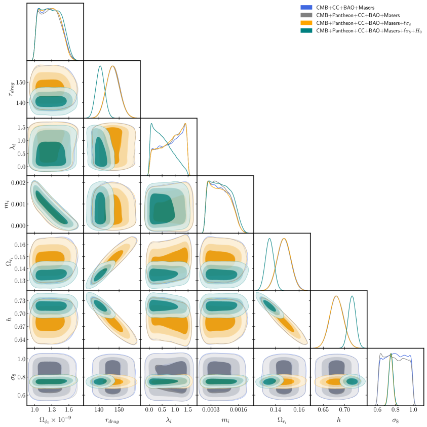
Figure 1: 68$\%$ and 95$\%$ CL contour plots and corresponding one-dimensional marginalized posterior distribution for all cosmological parameters obtained from the MCMC analysis within the present coupling scenario utilizing several combinations of data sets.

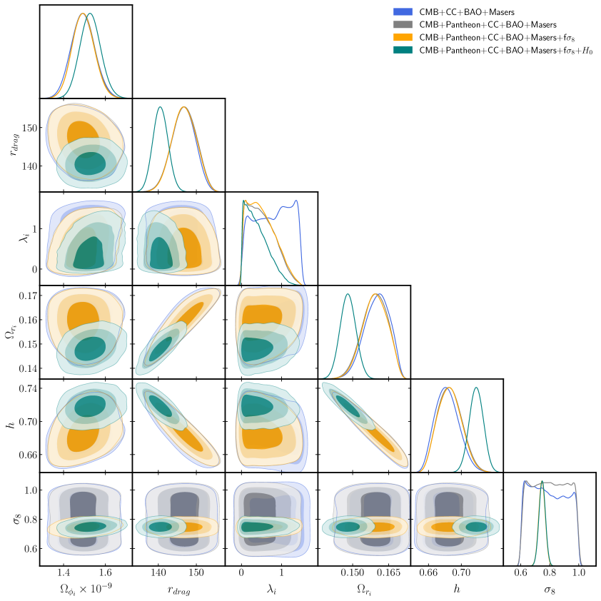
Figure 2: 68$\%$ and 95$\%$ CL contour plots and corresponding one-dimensional marginalized posterior distribution for all cosmological parameters obtained from the MCMC analysis for non-coupling scenario utilizing several combinations of data sets.

	Parameters	$\Omega_{dm}$	$r_{drag}$(Mpc)	$h$	$\Omega_{r_{0}}*10^{-5}$	$\sigma_{8}$
Data combinations	CMB+CC+BAO+MASERS	0.308${}^{+0.008}_{-0.007}$	147.09${}^{+3.304}_{-3.259}$	0.68$\pm$0.015	5.28${}^{+0.232}_{-0.231}$	0.80${}^{+0.136}_{-0.137}$
	CMB+Pantheon+CC+BAO+ MASERS	0.31$\pm$0.007	147.02${}^{+3.31}_{-3.32}$	0.684$\pm$0.015	5.24$\pm$0.226	0.80${}^{+0.136}_{-0.134}$
	CMB+Pantheon+CC+BAO+ MASERS+$f\sigma_{8}(z)$	0.306${}^{+0.007}_{-0.006}$	147.2${}^{+3.33}_{-3.34}$	0.683$\pm$0.015	5.26$\pm$0.227	0.73$\pm$0.021
	CMB+Pantheon+CC+BAO+ MASERS+$f\sigma_{8}(z)$+H0	0.303$\pm$0.0068	140.53${}^{+1.97}_{-1.95}$	0.72$\pm$0.0085	4.77$\pm$0.129	0.74$\pm$0.022

Table 3: Mean values with 68% confidence level (CL) errors on cosmological and free parameters within the $\Lambda$CDM paradigm from various data combinations.

We start by discussing the results obtained within the interacting canonical context. In table 2, we present the mean values and the 1$\sigma$ ranges of different cosmological parameters with both coupled and uncoupled scenarios.

To see the effect of the inclusion of each data set in the coupled scenario on the constraint of each parameter, we refer to Fig.1, where we show 1-dimensional marginalized posterior distributions and the corresponding 2D contour plots at 68$\%$ and 95$\%$ confidence level (CL) for all independent parameters. We gradually added Pantheon, $f\sigma_{8}$, and $H_{0}$ to the data set combination BAO + Masers + CMB + CC and can see more constrained parameters by adding more datasets. We also see a similar effect in the non-coupling case, as shown in Fig. 2. Since constraints on parameters show not much difference in the case of coupled or un-coupled scenarios, we, from now onward, focus on further studying the coupled case.

5.1 The $H_{0}$ and $\sigma_{8}$ Plane

We see that 1$\sigma$ confidence level contours are relatively larger for CMB + CC + BAO + Masers and CMB + Pantheon + CC + BAO + Masers data. Whereas the addition of $f\sigma_{8}$ and $H_{0}$ data strongly reduces the parameter space on parameter $\sigma_{8}$ and $h$, respectively. Interestingly, none of the parameters change their mean values except parameter $h$ when we add $H_{0}$ data from SH0ES or parameter $\sigma_{8}$ when we include $f\sigma_{8}$ data in the analysis.

In this study, we found that CMB + CC + BAO + Masers data combination shows $H_{0}$ = 68.1 $\pm$ 1.6 km/s/Mpc at 68$\%$ CL which is compatible well within 0.5$\sigma$ range with $H_{0}$ measurement from the joint result using TT,TE,EE + lowE + lensing in Planck (2018) under $\Lambda$CDM ($H_{0}$ = 67.37 $\pm$ 0.54 km/s/Mpc) [57]. But, the $H_{0}$ measurement from the same data combination shows 2$\sigma$ discrepancy with the prediction from SH0ES measurement in R21 ($H_{0}$ = 73.04 $\pm$ 1.01 km/s/Mpc) [81]. The consequent addition of Pantheon and growth rate data provides an identical estimate for the Hubble constant. However, the addition of $H_{0}$ data from SH0ES increases the difference to 3.5$\sigma$ with Planck (2018)+$\Lambda$CDM [57], we found that this value of $H_{0}$ is compatible within < 1$\sigma$ (mildly greater than 0.5$\sigma$) range with the value of the Hubble constant, $H_{0}$ = 73.04 $\pm$ 1.01 km/s/Mpc derived from the baseline fit with measurements from the latest SH0ES analysis in R21 [81].

Similarly, the matter fluctuation amplitude parameter $\sigma_{8}$ (also known as clustering parameter) is found to be well consistent within < 0.5$\sigma$ range with Planck (2018)+$\Lambda$CDM results ($\sigma_{8}$ = 0.8101 $\pm$ 0.0061) [57] for CMB + CC + BAO + Masers data set ($\sigma_{8}$ = 0.80 $\pm$ 0.133). We predict 0.3$\sigma$ compatibility with KiDS-1000-BOSS analysis ($\sigma_{8}$ = 0.760${}^{+0.021}_{-0.023}$ ) [95]. We also estimate 0.5$\sigma$ and 1$\sigma$ agreement with low redshift ($z\in$ [0.0, 0.55] ) and high redshift ($z\in$ [0.55, 1.5] ) DES-Y3 binned $\sigma_{8}(z)$ estimation [96], respectively. We must bear in mind that a good consistency with Planck (2018) and low-redshift DES-Y3 results come with an increase in the error bar of the parameter. Consequent addition of Pantheon data produces the identical estimate for the clustering parameter as above. However, the addition of priors from growth rate data reduces the clustering parameter, $\sigma_{8}$ to 0.748 $\pm$ 0.023 at 68$\%$ CL, in $\sim$2.5$\sigma$ tension with Planck (2018)+$\Lambda$CDM estimation. This prediction of $\sigma_{8}$ is at 0.3$\sigma$ agreement when compared with the KiDS-1000-BOSS predicted value [95]. Whereas the estimation is in good agreement with low-redshift and high-redshift DES-Y3 results at 0.1$\sigma$ and < 1$\sigma$ (mildly greater than 0.5$\sigma$), respectively [96]. The results from CMB + CC + BAO + Masers + Pantheon + $f\sigma_{8}(z)$ are more robust in tightening constraints on $\sigma_{8}$ parameter and justify the reduced uncertainty and the parameter space compared to the results from without growth rate data combination; see Table 2 and Fig.1. When additional data ($H_{0}$ from SH0ES measurement) are considered, the analysis remains unchanged.

5.2 The $h$-$r_{drag}$ Plane

In addition to a discrepancy in the Hubble constant, there is a discrepancy in the co-moving sound horizon at the end of the baryon drag epoch, $r_{drag}$ as well. The two parameters $H_{0}$ and $r_{drag}$ are strictly related when we consider BAO observations. In actuality, a combination of expansion history probes such as BAO and Pantheon data can provide a model-independent estimate of the low-redshift standard ruler, constraining the product of $h$ (with $H_{0}$= $h$ × 100 km/s/Mpc) and the sound horizon $r_{drag}$ directly. This implies that, to have a higher $H_{0}$ value in agreement with SH0ES, we need $r_{drag}$ $\sim$ 137 Mpc, while to agree with Planck, assuming $\Lambda$CDM, we need $r_{drag}$ $\sim$ 147 Mpc. For this reason, the solutions that increase the expansion rate and at the same time decrease $r_{drag}$ are most promising. In our analysis, this feature is completely in agreement with the Planck (2018) estimates due to the strong compatibility of estimated $H_{0}$ with the one from Planck (2018) + $\Lambda$CDM model. However, the addition of $H_{0}$ data that leads to the R21 value of $H_{0}$ also leads to an empirical determination of $r_{drag}$ near 140 Mpc. This modest discrepancy in the sound horizon value $r_{drag}$ from the one in [97] agrees with the slight discrepancy in the $H_{0}$ measurements from SH0ES. This correlation can also be seen from table 2. Evidently, this cosmological solution is promising and consistent with the fact that the relation $h$ - $r_{drag}$ is constant by the BAO measurements.

5.3 The $\sigma_{8}$- $\Omega_{dm}$ Plane

The model that allows larger $H_{0}$ values tend to introduce other tensions, such as higher $\sigma_{8}$ values. To obtain simultaneously higher values of $H_{0}$, lower values of $\sigma_{8}$, and consistent values of $\Omega_{dm}$ is also necessary to define the correct evolution. Since adding the BAO and SNe measurements to the Planck data strengthens the constraints towards Planck values, the correlation between their combined results is relatively strong. This is illustrated in Fig. 4. Adding $f{\sigma_{8}}$ results jointly with SH0ES improves the consistency with KiDS-1000-BOSS [95] and DES-Y3 [96] results and gives tighter constraint than other combinations. For this joint analysis, we found a slightly lower and constrained value for $\Omega_{dm}$, leading to a slightly lower but well-constrained value for $\sigma_{8}$ (Fig. 4). In summary, the analysis predicts the lower $\sigma_{8}$ and higher $H_{0}$ together, using the full combined likelihood for the data considered in this work.

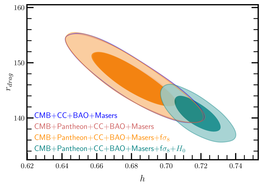
Figure 3: Constraints in the $h$-$r_{drag}$ plane from different combination of CMB, CC, BAO, Masers, Pantheon, growth and $H_{0}$ data (68% and 95% contours) in case of interacting model.

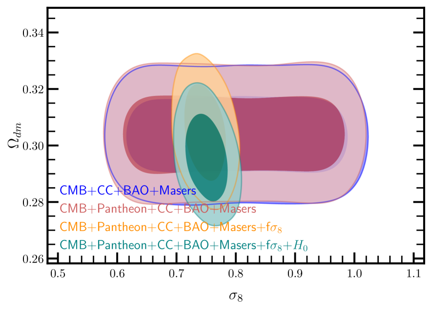
Figure 4: Marginalised constraints for the joint distributions of the fluctuation amplitude parameter $\sigma_{8}$ and dark matter density parameter $\Omega_{dm}$. The 68% and 95% credible regions are shown for different sets of CMB, SNIa, CC, BAO, Masers, $H_{0}$ and growth data for an interacting model.

5.4 The Co-moving Hubble Parameter

The recent BAO measurements along the line of sight and transverse directions lead to joint constraints on $H(z)r_{drag}$. Since Planck + $\Lambda$CDM constrains $r_{drag}$ to a precision of 0.2 %, the BAO measurements can be accurately converted into absolute measurements of H(z). These constraints on $H(z)$ from the BOSS analyses are plotted in Fig. 6. The error bars are constraints from BOSS DR12 galaxy sample [87], eBOSS DR14 quasar sample [85], the correlations of Ly$\alpha$ absorption in eBOSS DR14 at $z=2.34$ [98] and from the Ly$\alpha$ auto-correlation and cross-correlation with quasars from SDSS data release DR12 [86]. The error bar at $z=0$ shows the inferred distance-ladder Hubble measurement from R21 [81].

The illustration in Fig. 6 shows clearly how well the dark energy interaction model fits the BAO measurements of the Hubble parameter except for the DR12 $Ly$-$\alpha$ data point. It is also consistent with the R21 measurements of Hubble at $z=0$ for all the data sets combined in this work within one sigma error bars. This is also illustrated in Fig. 6, which shows the combined constraints on $h$ and $\Omega_{dm}$ from different data combinations. Without adding H0 to the combination of datasets BAO, Pantheon, $H(z)$ and Masers as seen in table 2, the tension with SH0ES measurement of $H_{0}$ still prevails. However, adding SH0ES data (green contour) constrain $\Omega_{dm}$ towards slightly lower values and shifts $H_{0}$ closer to the R21 measurement.

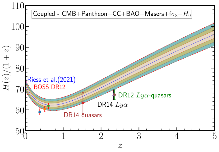
Figure 5: Co-moving Hubble parameter as a function of redshift, clearly showing the onset of acceleration just before the redshift around $z$ = 0.6, reconstructed using a combination of CMB, SNIa, CC, BAO, Masers, $H_{0}$ and growth data for interacting model. The solid blue line shows the best-fit reconstructed results, while the outer regions show results within 1$\sigma$, 2$\sigma$, 3$\sigma$ CL separated by orange, pink and red-dashed lines.

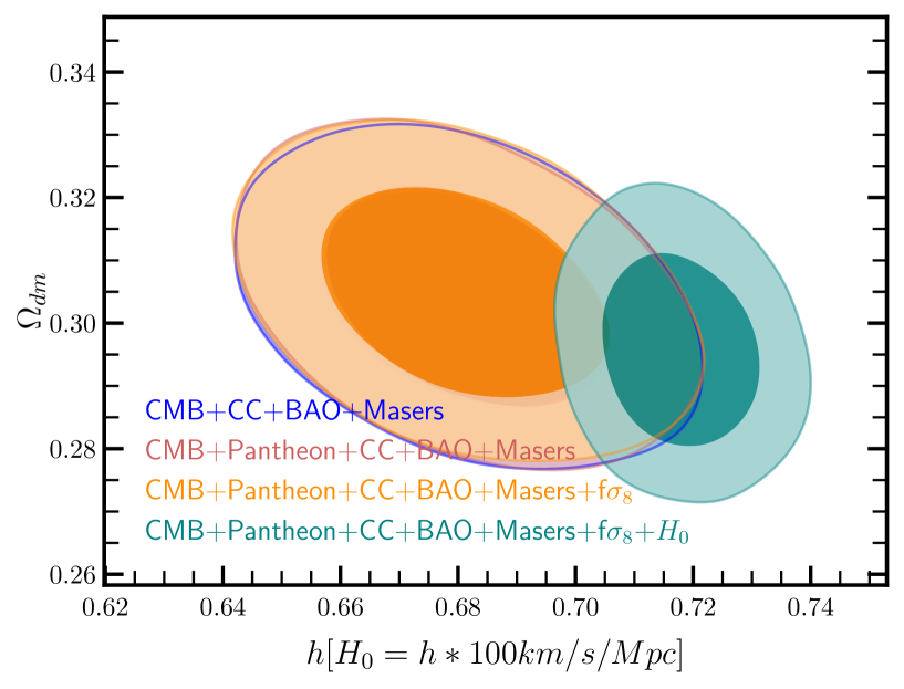
Figure 6: The CMB + SNIa + CC + BAO + Masers + $f{\sigma_{8}}$ + $H_{0}$ data constraints on $h$ and $\Omega_{dm}$ in the coupled model, compared to the results from without $H_{0}$ data. Adding SH0ES $H_{0}$ constrains the Hubble parameter, comparable to that R21 estimation. Darker and lighter contours show 68% and 95% of the probability, respectively.

5.5 Other Cosmological Parameters

We further analyse the model for completeness’ sake and clarity. We have plotted the energy density evolution parameter for dark energy and dark matter, along with 68% and 95% CL for the coupled case using all the data presented in this work in Fig. 8. Fig. 8 shows the overlapping confidence contours for the equation of state parameter as a function of redshift from coupled and uncoupled models using all the data presented in this work. The solid yellow and red lines indicate the best-fit values for the DE EoS parameter for coupled and uncoupled models, respectively. However, Fig. 9 shows the density parameters and equation of state parameters evolution from their best-fit values as a function of the logarithmic scale factor. These analyses exactly show the expected behaviour of the observed universe at present, which is dark energy-dominated accelerated expansion. Moreover, while fitting with the data, we found that the model favors small values of the coupling parameter $``$Q”, making the parameter evolution indistinguishable compared to the one from the uncoupled case. However, these predictions are model-dependent and may vary for other coupling models.

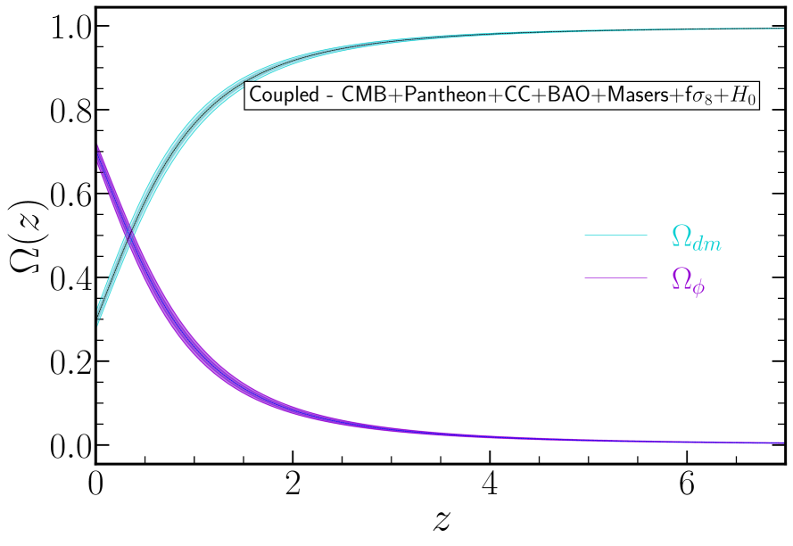
Figure 7: The 68% and 95% CL along with the mean value for relative energy density parameters $\Omega_{dm}$ (cyan) and $\Omega_{\phi}$ (purple) for the coupled model with respect to redshift $(z)$. The evolution is plotted for all the data combined together, considered in this work. The black-dashed and blue-dashed lines corresponds to the best-fit values of DM and DE density parameters.

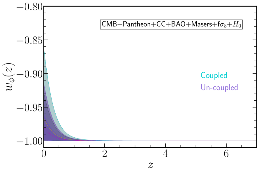
Figure 8: Evolution of dark energy equation of state parameter with respect to redshift $(z)$ for coupled and un-coupled scenario. The solid yellow line shows the best fit result while the outer blue and cyan regions show the 1$\sigma$ and 2$\sigma$ CL for coupled case. The solid red line shows the best fit result while the outer purple regions show the 1$\sigma$ and 2$\sigma$ CL for un-coupled case.

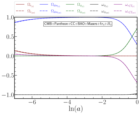
Figure 9: The best-fit evolution of key cosmological parameters for the coupled and uncoupled models is shown for the combined set of CMB, SNIa, CC, BAO, Masers, $H_{0}$, and growth data. The solid lines and dashed-dot lines show the evolution in the coupled case and un-coupled case, respectively.

5.6 Comparison with $\Lambda$CDM results

In Table 3, we present the constraints that we got from $\chi^{2}$ minimization fitting assuming the standard $\Lambda$CDM model. We also show how best-fit values change within the same model in addition to different datasets. Including growth data constrain $\sigma_{8}$ parameter compared to $``$CMB + Pantheon + CC + BAO + Masers” data set. It does not affect the constraints on other cosmological parameters. On further inclusion of local $H_{0}$ value from SH0ES et al.[99], the best-fit value of $h$ shifts towards Riess et al. value [13] and the error bar gets smaller too when related to without SH0ES data set. The effect of the shift in $h$ can also be seen in $r_{drag}$ parameter values (both best-fit and error bars). Because of cosmic chronometer data, we expect a co-relation between $h-\Omega_{dm}$. That effect can also be seen in the $``$CMB + Pantheon + CC + BAO + Masers + $f\sigma_{8}(z)+H_{0}$” case, how constraints on $\Omega_{dm}$ changes due to change of best-fit of $h$ and $r_{drag}$ as compared to $``$CMB + Pantheon + CC + BAO + Masers + $f\sigma_{8}(z)$” case. From Fig. 1, 4, 6 and Table 3, we can see that constraints on cosmological parameters do not vary much from $\Lambda$CDM bounds to interacting DE $-$ DM model bounds.

5.7 Model Selection Statistics

In this section, we discuss the comparison of our models (coupled and uncoupled) with the standard $\Lambda$CDM model. The $\Lambda$CDM model corresponds to the dark energy equation of state -1, whereas in our model, the dark energy equation of state is allowed to vary. One way to compare these dark energy models is Akaike Information Criterion (AIC), where AIC is defined as AIC = $\chi^{2}_{min}$ + 2 $\cdot$ d. Another way is Bayesian Information Criterion (BIC), where BIC is defined as BIC = $\chi^{2}_{min}$ + d $\cdot$ ln$(N)$. $\chi^{2}_{min}$ is the chi-squared minimization to measure how well the data fit a model. $`$d’ is the number of parameters in the model and $`N$’ is the number of observational data points. The lowest chi-squared and lowest AIC or BIC at each point indicate where the parameters and model most closely match the measured data. Comparing both the methods, we can see from table 4 that there is always an improvement in $\chi^{2}_{min}$ value for the coupled model when compared to the un-coupled or $\Lambda$CDM model. For all the data together, this leads to a large reduction in AIC and BIC estimates for the coupled model, and hence, the same is significantly preferred over the $\Lambda$CDM model.

We also considered $\chi^{2}_{min}$ per number of degrees of freedom approach for the present model, aiming to understand the observational solidity of the model with respect to the standard reference model. We found that $\frac{\chi^{2}_{min}}{n_{dof}}$ raises an overfitting issue with the coupled model opposing the analysis from AIC. This trait can be found in Table 4. However, using $\frac{\chi^{2}_{min}}{n_{dof}}$ method, it is clear that the $\Lambda$CDM model has the goodness of fit (GoF) to the data and hence, is the favoured model. In summary, from the point of view of the $\frac{\chi^{2}_{min}}{n_{dof}}$ analysis, $\Lambda$CDM is still a preferred candidate but from the perspective of AIC and BIC analyses, coupled cosmology is the preferred scenario for the universe’s evolution.

Model	$\chi^{2}_{min}$	$\frac{\chi^{2}_{min}}{n_{dof}}$	d	N	AIC	BIC	$\Delta$ AIC	$\Delta$ BIC
Coupled	43.25	0.697	7	69	57.25	72.89	10.64	6.17
Un-coupled	48.40	0.768	6	69	60.40	73.80	7.49	5.26
$\Lambda$CDM	57.89	0.904	5	69	67.89	79.06	0.0	0.0

Table 4: The $\chi^{2}_{min}$, AIC and BIC estimation for coupled/un-coupled and $\Lambda$CDM model for the combination of all data set.

6 Final Remarks

In this work, we study an interacting dark energy-dark matter model having time-varying interaction term $Q=F,_{\phi}\rho_{dm}\dot{\phi}$. This work is interesting because it is theoretically very well motivated from a field theory perspective, not just phenomenological. We can see that because of the time-varying interaction term, the dark energy component may differ from the cosmological constant at very early times ($z=1100$). Also, a small interaction is not disfavoured by the data at late times.

Initially, we tested our model to find the future attractor solution by formatting a coupled dynamical set of equations. Later, we subjected the model to various data combinations and tried to understand better the influence of each cosmological data set on respective cosmological parameters.

We found that while using all the datasets together, we found $H_{0}$ value to be in excellent agreement with the latest local determination by R21 [81], though in substantial ($\sim 3.5\sigma$) tension with Planck [57] measurements. It is widely discussed that the models that alleviate the $H_{0}$ discrepancy do not necessarily solve other tensions, such as a higher value of $\sigma_{8}$. Similarly, in our work, we found that the coupled model provides a remarkably better fit to the CMB, CC, BAO, Masers, $f\sigma_{8}$ and $H_{0}$ in combination with each other and predicts a (lower) late-time clustering parameter $\sigma_{8}$ = $0.75\pm 0.023$. The $\sigma_{8}$ value is in good agreement with KiDS-1000-BOSS and DES-Y3 low- and high-redshift estimations, although in moderate tension with Planck 2018 + $\Lambda$CDM results which prefer a roughly $2.5\sigma$ higher value of $\sigma_{8}$ compared to our model prediction.

We also emphasize the parameters like the sound horizon at the drag epoch $r_{drag}$ and the dark matter energy density $\Omega_{dm}$, and their respective correlations, in terms of $h$-$r_{drag}$ and $\sigma_{8}$-$\Omega_{dm}$ planes. The findings predicted the smaller value of $r_{drag}$ for a larger value of $H_{0}$ at the cost of increasing disagreement with the Planck data. Moreover, the results from the $\sigma_{8}$-$\Omega_{dm}$ parameter space showed marginal tension with Planck with lower and substantially constrained values of $\sigma_{8}$ and $\Omega_{dm}$ for all the combined data in this work. The illustration in Fig. 6 clearly showed some disagreement ($\sim$ 3$\sigma$) with high-redshift BAO measurements from quasar Ly$\alpha$ observations. The interacting model confirms the overall good consistency of reconstructed $H(z)$ with combined BAO measurements of $H(z)$. Later, we also presented the time evolution of key cosmological parameters along with their confidence ranges for the coupled cosmological model. We found no significant distinction in the parameter evolution compared with the uncoupled scenario due to very low coupling parameter values preferred by the cosmological datasets. Later, we also presented the time evolution of density parameters, the equation of state parameters, and their two-sigma confidence region for the coupled cosmological model.

We then discussed the model comparison techniques to measure the goodness of fit of a given model to the data. We found that introducing extra parameters improves the fit determined by AIC and BIC and strongly favors a complex, coupled model over the $\Lambda$CDM one. Moreover, this model introduces two extra parameters, so the $``$weighted” chi-square test favors the $\Lambda$CDM for all the combined data. Such inconsistencies and discrepancies motivate us to look further for the best theoretical model to describe the universe. Following the above analyses, these differences could signify either the need for new exotic dark energy physics to withstand the data or new observations to improve the quality of the data.

In the near future, we shall extend our analysis to incorporate one extra element which can mimic phantom dark energy at present, along with the already present interacting dark matter-dark energy scenarios to resolve present cosmological tensions.

References

- [1] S. Perlmutter et al., “Discovery of a supernova explosion at half the age of the Universe and its cosmological implications,” Nature, vol. 391, pp. 51–54, 1998.
- [2] A. G. Riess et al., “Observational evidence from supernovae for an accelerating universe and a cosmological constant,” Astron. J., vol. 116, pp. 1009–1038, 1998.
- [3] S. Perlmutter et al., “Measurements of and from 42 high redshift supernovae,” Astrophys. J., vol. 517, pp. 565–586, 1999.
- [4] P. J. E. Peebles and B. Ratra, “The Cosmological Constant and Dark Energy,” Rev. Mod. Phys., vol. 75, pp. 559–606, 2003.
- [5] A. G. Riess, L.-G. Sirolger, J. Tonry, S. Casertano, H. C. Ferguson, B. Mobasher, P. Challis, A. V. Filippenko, S. Jha, W. Li, R. Chornock, R. P. Kirshner, B. Leibundgut, M. Dickinson, M. Livio, M. Giavalisco, C. C. Steidel, T. Benítez, and Z. Tsvetanov, “Type ia supernova discoveries at z > 1 from the hubble space telescope: Evidence for past deceleration and constraints on dark energy evolution,” Astrophysical Journal Letters, vol. 607, no. 2 I, p. 665 – 687, 2004. Cited by: 3258; All Open Access, Bronze Open Access, Green Open Access.
- [6] P. Astier, J. Guy, N. Regnault, R. Pain, E. Aubourg, D. Balam, S. Basa, R. Carlberg, S. Fabbro, F. Dominique, I. Hook, D. Howell, H. Lafoux, J. Neill, N. Palanque-Delabrouille, K. Perrett, C. Pritchet, J. Rich, M. Sullivan, and N. Walton, “The supernova legacy survey: measurement of , and w from the first year data set,” http://dx.doi.org/10.1051/0004-6361:20054185, vol. 447, 10 2005.
- [7] D. J. Eisenstein, I. Zehavi, D. W. Hogg, R. Scoccimarro, M. R. Blanton, R. C. Nichol, R. Scranton, H.-J. Seo, M. Tegmark, Z. Zheng, et al., “Detection of the baryon acoustic peak in the large-scale correlation function of sdss luminous red galaxies,” The Astrophysical Journal, vol. 633, no. 2, p. 560, 2005.
- [8] C. J. MacTavish, P. A. R. Ade, J. J. Bock, J. R. Bond, J. Borrill, A. Boscaleri, P. Cabella, C. R. Contaldi, B. P. Crill, P. de Bernardis, G. D. Gasperis, A. de Oliveira-Costa, G. D. Troia, G. di Stefano, E. Hivon, A. H. Jaffe, W. C. Jones, T. S. Kisner, A. E. Lange, A. M. Lewis, S. Masi, P. D. Mauskopf, A. Melchiorri, T. E. Montroy, P. Natoli, C. B. Netterfield, E. Pascale, F. Piacentini, D. Pogosyan, G. Polenta, S. Prunet, S. Ricciardi, G. Romeo, J. E. Ruhl, P. Santini, M. Tegmark, M. Veneziani, and N. Vittorio, “Cosmological parameters from the 2003 flight of boomerang,” The Astrophysical Journal, vol. 647, p. 799, aug 2006.
- [9] E. Komatsu, J. Dunkley, M. R. Nolta, C. L. Bennett, B. Gold, G. Hinshaw, N. Jarosik, D. Larson, M. Limon, L. Page, D. N. Spergel, M. Halpern, R. S. Hill, A. Kogut, S. S. Meyer, G. S. Tucker, J. L. Weiland, E. Wollack, and E. L. Wright, “Five-year wilkinson microwave anisotropy probe* observations: Cosmological interpretation,” The Astrophysical Journal Supplement Series, vol. 180, p. 330, feb 2009.
- [10] M. Tegmark, M. A. Strauss, M. R. Blanton, K. Abazajian, S. Dodelson, H. Sandvik, X. Wang, D. H. Weinberg, I. Zehavi, N. A. Bahcall, et al., “Cosmological parameters from sdss and wmap,” Physical review D, vol. 69, no. 10, p. 103501, 2004.
- [11] G. Hinshaw, J. L. Weiland, R. S. Hill, N. Odegard, D. Larson, C. L. Bennett, J. Dunkley, B. Gold, M. R. Greason, N. Jarosik, E. Komatsu, M. R. Nolta, L. Page, D. N. Spergel, E. Wollack, M. Halpern, A. Kogut, M. Limon, S. S. Meyer, G. S. Tucker, and E. L. Wright, “Five-year wilkinson microwave anisotropy probe* observations: Data processing, sky maps, and basic results,” The Astrophysical Journal Supplement Series, vol. 180, p. 225, feb 2009.
- [12] G. Risaliti and E. Lusso, “Cosmological constraints from the Hubble diagram of quasars at high redshifts,” Nature Astron., vol. 3, no. 3, pp. 272–277, 2019.
- [13] A. G. Riess, W. Yuan, L. M. Macri, D. Scolnic, D. Brout, S. Casertano, D. O. Jones, Y. Murakami, G. S. Anand, L. Breuval, T. G. Brink, A. V. Filippenko, S. Hoffmann, S. W. Jha, W. D. Kenworthy, J. Mackenty, B. E. Stahl, and W. Zheng, “A comprehensive measurement of the local value of the hubble constant with 1 km/s/mpc uncertainty from the hubble space telescope and the sh0es team,” The Astrophysical Journal Letters, vol. 934, p. L7, jul 2022.
- [14] S. Capozziello, Ruchika, and A. A. Sen, “Model independent constraints on dark energy evolution from low-redshift observations,” Mon. Not. Roy. Astron. Soc., vol. 484, p. 4484, 2019.
- [15] E. J. Copeland, M. Sami, and S. Tsujikawa, “Dynamics of dark energy,” Int. J. Mod. Phys. D, vol. 15, pp. 1753–1936, 2006.
- [16] P. Bull et al., “Beyond CDM: Problems, solutions, and the road ahead,” Phys. Dark Univ., vol. 12, pp. 56–99, 2016.
- [17] L. Perivolaropoulos and F. Skara, “Challenges for CDM: An update,” New Astron. Rev., vol. 95, p. 101659, 2022.
- [18] N. Schöneberg, G. Franco Abellán, A. Pérez Sánchez, S. J. Witte, V. Poulin, and J. Lesgourgues, “The H0 Olympics: A fair ranking of proposed models,” Phys. Rept., vol. 984, pp. 1–55, 2022.
- [19] I. Zlatev, L.-M. Wang, and P. J. Steinhardt, “Quintessence, cosmic coincidence, and the cosmological constant,” Phys. Rev. Lett., vol. 82, pp. 896–899, 1999.
- [20] T. Chiba, T. Okabe, and M. Yamaguchi, “Kinetically driven quintessence,” Phys. Rev. D, vol. 62, p. 023511, 2000.
- [21] R. de Putter and E. V. Linder, “Kinetic k-essence and Quintessence,” Astropart. Phys., vol. 28, pp. 263–272, 2007.
- [22] P. F. Gonzalez-Diaz, “Cosmological models from quintessence,” Phys. Rev. D, vol. 62, p. 023513, 2000.
- [23] T. Duary, A. D. N. Banerjee, and N. Banerjee, “Thawing and Freezing Quintessence Models: A thermodynamic Consideration,” Eur. Phys. J. C, vol. 79, no. 11, p. 888, 2019.
- [24] R. R. Caldwell and E. V. Linder, “The Limits of quintessence,” Phys. Rev. Lett., vol. 95, p. 141301, 2005.
- [25] S. M. Carroll, “Quintessence and the rest of the world: Suppressing long-range interactions,” Phys. Rev. Lett., vol. 81, pp. 3067–3070, Oct 1998.
- [26] T. Barreiro, O. Bertolami, and P. Torres, “Gamma-Ray Bursts and Dark Energy - Dark Matter interaction,” Mon. Not. Roy. Astron. Soc., vol. 409, pp. 750–754, 2010.
- [27] W. Yang, S. Pan, and A. Paliathanasis, “Cosmological constraints on an exponential interaction in the dark sector,” Monthly Notices of the Royal Astronomical Society, vol. 482, pp. 1007–1016, 10 2018.
- [28] R. An, C. Feng, and B. Wang, “Relieving the tension between weak lensing and cosmic microwave background with interacting dark matter and dark energy models,” Journal of Cosmology and Astroparticle Physics, vol. 2018, p. 038, feb 2018.
- [29] W. Yang, N. Banerjee, and S. Pan, “Constraining a dark matter and dark energy interaction scenario with a dynamical equation of state,” Phys. Rev. D, vol. 95, no. 12, p. 123527, 2017. [Addendum: Phys.Rev.D 96, 089903 (2017)].
- [30] S. Fay, “Constraints from growth-rate data on some coupled dark energy models mimicking a CDM expansion,” Mon. Not. Roy. Astron. Soc., vol. 460, no. 2, pp. 1863–1868, 2016.
- [31] W. Yang and L. Xu, “Testing coupled dark energy with large scale structure observation,” JCAP, vol. 08, p. 034, 2014.
- [32] A. Piloyan, V. Marra, M. Baldi, and L. Amendola, “Linear perturbation constraints on multi-coupled dark energy,” Journal of Cosmology and Astroparticle Physics, vol. 2014, p. 045, feb 2014.
- [33] Y.-H. Li and X. Zhang, “Large-scale stable interacting dark energy model: Cosmological perturbations and observational constraints,” Phys. Rev. D, vol. 89, no. 8, p. 083009, 2014.
- [34] W. Yang, S. Pan, E. Di Valentino, R. C. Nunes, S. Vagnozzi, and D. F. Mota, “Tale of stable interacting dark energy, observational signatures, and the tension,” JCAP, vol. 09, p. 019, 2018.
- [35] E. Di Valentino, A. Melchiorri, O. Mena, and S. Vagnozzi, “Interacting dark energy in the early 2020s: A promising solution to the and cosmic shear tensions,” Phys. Dark Univ., vol. 30, p. 100666, 2020.
- [36] E. Di Valentino, A. Melchiorri, O. Mena, S. Pan, and W. Yang, “Interacting Dark Energy in a closed universe,” Mon. Not. Roy. Astron. Soc., vol. 502, no. 1, pp. L23–L28, 2021.
- [37] A. Gómez-Valent, Z. Zheng, L. Amendola, C. Wetterich, and V. Pettorino, “Coupled and uncoupled early dark energy, massive neutrinos, and the cosmological tensions,” Phys. Rev. D, vol. 106, no. 10, p. 103522, 2022.
- [38] B. M. Jackson, A. Taylor, and A. Berera, “On the large-scale instability in interacting dark energy and dark matter fluids,” Phys. Rev. D, vol. 79, p. 043526, Feb 2009.
- [39] W. Zimdahl and D. Pavon, “Interacting quintessence,” Phys. Lett. B, vol. 521, pp. 133–138, 2001.
- [40] M. S. Linton, A. Pourtsidou, R. Crittenden, and R. Maartens, “Variable sound speed in interacting dark energy models,” JCAP, vol. 04, p. 043, 2018.
- [41] G. Olivares, F. Atrio-Barandela, and D. Pavon, “Matter density perturbations in interacting quintessence models,” Phys. Rev. D, vol. 74, p. 043521, 2006.
- [42] B. Wang, E. Abdalla, F. Atrio-Barandela, and D. Pavón, “Dark matter and dark energy interactions: theoretical challenges, cosmological implications and observational signatures,” Reports on Progress in Physics, vol. 79, p. 096901, aug 2016.
- [43] J. Valiviita, E. Majerotto, and R. Maartens, “Instability in interacting dark energy and dark matter fluids,” JCAP, vol. 07, p. 020, 2008.
- [44] D. G. A. Duniya, D. Bertacca, and R. Maartens, “Probing the imprint of interacting dark energy on very large scales,” Phys. Rev. D, vol. 91, p. 063530, Mar 2015.
- [45] C. Carbone, M. Baldi, V. Pettorino, and C. Baccigalupi, “Maps of CMB lensing deflection from N-body simulations in Coupled Dark Energy Cosmologies,” JCAP, vol. 09, p. 004, 2013.
- [46] L. Amendola and D. Tocchini-Valentini, “Perturbations growth and bias during acceleration,” in 37th Rencontres de Moriond on the Cosmological Model, pp. 407–410, 5 2002.
- [47] E. R. M. Tarrant, C. van de Bruck, E. J. Copeland, and A. M. Green, “Coupled quintessence and the halo mass function,” Phys. Rev. D, vol. 85, p. 023503, Jan 2012.
- [48] J.-H. He and B. Wang, “Effects of the interaction between dark energy and dark matter on cosmological parameters,” Journal of Cosmology and Astroparticle Physics, vol. 2008, p. 010, jun 2008.
- [49] J. B. Binder and G. M. Kremer, “Model for a universe described by a non-minimally coupled scalar field and interacting dark matter,” Gen. Rel. Grav., vol. 38, pp. 857–870, 2006.
- [50] T. Patil, S. Panda, M. Sharma, and Ruchika, “Dynamics of interacting scalar field model in the realm of chiral cosmology,” Eur. Phys. J. C, vol. 83, no. 2, p. 131, 2023.
- [51] C. van de Bruck, J. Mifsud, J. P. Mimoso, and N. J. Nunes, “Generalized dark energy interactions with multiple fluids,” JCAP, vol. 11, p. 031, 2016.
- [52] T. S. Koivisto and N. J. Nunes, “Inflation and dark energy from three-forms,” Phys. Rev. D, vol. 80, p. 103509, 2009.
- [53] A. R. Gomes and L. Amendola, “The general form of the coupled Horndeski Lagrangian that allows cosmological scaling solutions,” JCAP, vol. 02, p. 035, 2016.
- [54] T. S. Koivisto and N. J. Nunes, “Coupled three-form dark energy,” Phys. Rev. D, vol. 88, p. 123512, Dec 2013.
- [55] T. S. Koivisto and N. J. Nunes, “Three-form cosmology,” Phys. Lett. B, vol. 685, pp. 105–109, 2010.
- [56] B. J. Barros and N. J. Nunes, “Three-form inflation in type II Randall-Sundrum,” Phys. Rev. D, vol. 93, no. 4, p. 043512, 2016.
- [57] N. Aghanim et al., “Planck 2018 results. VI. Cosmological parameters,” Astron. Astrophys., vol. 641, p. A6, 2020. [Erratum: Astron.Astrophys. 652, C4 (2021)].
- [58] D. Dutcher et al., “Measurements of the E-mode polarization and temperature-E-mode correlation of the CMB from SPT-3G 2018 data,” Phys. Rev. D, vol. 104, no. 2, p. 022003, 2021.
- [59] S. Aiola et al., “The Atacama Cosmology Telescope: DR4 Maps and Cosmological Parameters,” JCAP, vol. 12, p. 047, 2020.
- [60] L. Verde, T. Treu, and A. G. Riess, “Tensions between the Early and the Late Universe,” Nature Astron., vol. 3, p. 891, 7 2019.
- [61] J. Evslin, A. A. Sen, and Ruchika, “Price of shifting the Hubble constant,” Phys. Rev. D, vol. 97, no. 10, p. 103511, 2018.
- [62] S. Kumar and R. C. Nunes, “Echo of interactions in the dark sector,” Phys. Rev. D, vol. 96, no. 10, p. 103511, 2017.
- [63] W. Yang, A. Mukherjee, E. Di Valentino, and S. Pan, “Interacting dark energy with time varying equation of state and the tension,” Phys. Rev. D, vol. 98, no. 12, p. 123527, 2018.
- [64] E. Di Valentino, O. Mena, S. Pan, L. Visinelli, W. Yang, A. Melchiorri, D. F. Mota, A. G. Riess, and J. Silk, “In the realm of the Hubble tension—a review of solutions,” Class. Quant. Grav., vol. 38, no. 15, p. 153001, 2021.
- [65] F. Okamatsu, T. Sekiguchi, and T. Takahashi, “ tension without CMB data: Beyond the CDM,” Phys. Rev. D, vol. 104, no. 2, p. 023523, 2021.
- [66] E. Di Valentino et al., “Cosmology Intertwined III: and ,” Astropart. Phys., vol. 131, p. 102604, 2021.
- [67] V. Salvatelli, N. Said, M. Bruni, A. Melchiorri, and D. Wands, “Indications of a late-time interaction in the dark sector,” Phys. Rev. Lett., vol. 113, no. 18, p. 181301, 2014.
- [68] J. Väliviita and E. Palmgren, “Distinguishing interacting dark energy from wCDM with CMB, lensing, and baryon acoustic oscillation data,” JCAP, vol. 07, p. 015, 2015.
- [69] R. C. Nunes, S. Pan, and E. N. Saridakis, “New constraints on interacting dark energy from cosmic chronometers,” Phys. Rev. D, vol. 94, no. 2, p. 023508, 2016.
- [70] E. Marachlian, I. E. Sánchez G., and O. P. Santillán, “Emergent Universe as an interaction in the dark sector,” Mod. Phys. Lett. A, vol. 32, no. 28, p. 1750152, 2017.
- [71] L. Knox and M. Millea, “Hubble constant hunter’s guide,” Phys. Rev. D, vol. 101, no. 4, p. 043533, 2020.
- [72] E. Di Valentino et al., “Snowmass2021 - Letter of interest cosmology intertwined II: The hubble constant tension,” Astropart. Phys., vol. 131, p. 102605, 2021.
- [73] A. A. Sen, S. A. Adil, and S. Sen, “Do cosmological observations allow a negative ?,” Mon. Not. Roy. Astron. Soc., vol. 518, no. 1, pp. 1098–1105, 2022.
- [74] L. A. Escamilla, O. Akarsu, E. Di Valentino, and J. A. Vazquez, “Model-independent reconstruction of the Interacting Dark Energy Kernel: Binned and Gaussian process,” 2023.
- [75] S. A. Adil, O. Akarsu, E. Di Valentino, R. C. Nunes, E. Ozulker, A. A. Sen, and E. Specogna, “Omnipotent dark energy: A phenomenological answer to the Hubble tension,” 2023.
- [76] L. Amendola, “Coupled quintessence,” Phys. Rev. D, vol. 62, p. 043511, Jul 2000.
- [77] L. Amendola and D. Tocchini-Valentini, “Baryon bias and structure formation in an accelerating universe,” Phys. Rev. D, vol. 66, p. 043528, 2002.
- [78] T. Damour and C. Gundlach, “Nucleosynthesis constraints on an extended jordan-brans-dicke theory,” Phys. Rev. D, vol. 43, pp. 3873–3877, Jun 1991.
- [79] L. Chen, Q.-G. Huang, and K. Wang, “Distance Priors from Planck Final Release,” JCAP, vol. 02, p. 028, 2019.
- [80] P. A. R. Ade et al., “Planck 2015 results. XIV. Dark energy and modified gravity,” Astron. Astrophys., vol. 594, p. A14, 2016.
- [81] A. G. Riess et al., “A Comprehensive Measurement of the Local Value of the Hubble Constant with 1 km/s/Mpc Uncertainty from the Hubble Space Telescope and the SH0ES Team,” Astrophys. J. Lett., vol. 934, no. 1, p. L7, 2022.
- [82] A. Gómez-Valent and L. Amendola, “ from cosmic chronometers and Type Ia supernovae, with Gaussian Processes and the novel Weighted Polynomial Regression method,” JCAP, vol. 04, p. 051, 2018.
- [83] F. Beutler et al., “The 6df galaxy survey: baryon acoustic oscillations and the local hubble constant,” Monthly Notices of the Royal Astronomical Society, vol. 416, pp. 3017–3032, jul 2011.
- [84] A. J. Ross, L. Samushia, C. Howlett, W. J. Percival, A. Burden, and M. Manera, “The clustering of the SDSS DR7 main Galaxy sample – I. A 4 per cent distance measure at ,” Mon. Not. Roy. Astron. Soc., vol. 449, no. 1, pp. 835–847, 2015.
- [85] M. Ata et al., “The clustering of the SDSS-IV extended Baryon Oscillation Spectroscopic Survey DR14 quasar sample: first measurement of baryon acoustic oscillations between redshift 0.8 and 2.2,” Mon. Not. Roy. Astron. Soc., vol. 473, no. 4, pp. 4773–4794, 2018.
- [86] H. du Mas des Bourboux et al., “Baryon acoustic oscillations from the complete SDSS-III Ly-quasar cross-correlation function at ,” Astron. Astrophys., vol. 608, p. A130, 2017.
- [87] S. Alam et al., “The clustering of galaxies in the completed SDSS-III Baryon Oscillation Spectroscopic Survey: cosmological analysis of the DR12 galaxy sample,” Mon. Not. Roy. Astron. Soc., vol. 470, no. 3, pp. 2617–2652, 2017.
- [88] M. J. Reid, J. A. Braatz, J. J. Condon, L. J. Greenhill, C. Henkel, and K. Y. Lo, “The megamaser cosmology project. i. very long baseline interferometric observations of ugc 3789,” The Astrophysical Journal, vol. 695, p. 287, mar 2009.
- [89] J. A. Braatz, M. J. Reid, E. M. L. Humphreys, C. Henkel, J. J. Condon, and K. Lo, “The megamaser cosmology project. ii. the angular-diameter distance to ugc 3789,” The Astrophysical Journal, vol. 718, p. 657, jul 2010.
- [90] M. J. Reid, J. A. Braatz, J. J. Condon, K. Y. Lo, C. Y. Kuo, C. M. V. Impellizzeri, and C. Henkel, “The megamaser cosmology project. iv. a direct measurement of the hubble constant from ugc 3789,” The Astrophysical Journal, vol. 767, p. 154, apr 2013.
- [91] C. Y. Kuo, J. A. Braatz, M. J. Reid, K. Y. Lo, J. J. Condon, C. M. V. Impellizzeri, and C. Henkel, “The megamaser cosmology project. v. an angular-diameter distance to ngc 6264 at 140 mpc,” The Astrophysical Journal, vol. 767, p. 155, apr 2013.
- [92] F. Gao, J. A. Braatz, M. J. Reid, K. Y. Lo, J. J. Condon, C. Henkel, C. Y. Kuo, C. M. V. Impellizzeri, D. W. Pesce, and W. Zhao, “The megamaser cosmology project. viii. a geometric distance to ngc 5765b,” The Astrophysical Journal, vol. 817, p. 128, jan 2016.
- [93] S. Basilakos, S. Nesseris, and L. Perivolaropoulos, “Observational constraints on viable f(R) parametrizations with geometrical and dynamical probes,” Phys. Rev. D, vol. 87, no. 12, p. 123529, 2013.
- [94] D. Foreman-Mackey, D. W. Hogg, D. Lang, and J. Goodman, “emcee: The mcmc hammer,” Publications of the Astronomical Society of the Pacific, vol. 125, p. 306, feb 2013.
- [95] C. Heymans et al., “KiDS-1000 Cosmology: Multi-probe weak gravitational lensing and spectroscopic galaxy clustering constraints,” Astron. Astrophys., vol. 646, p. A140, 2021.
- [96] T. M. C. Abbott et al., “Dark Energy Survey Year 3 results: Constraints on extensions to CDM with weak lensing and galaxy clustering,” Phys. Rev. D, vol. 107, no. 8, p. 083504, 2023.
- [97] J. L. Bernal, L. Verde, and A. G. Riess, “The trouble with ,” JCAP, vol. 10, p. 019, 2016.
- [98] V. de Sainte Agathe et al., “Baryon acoustic oscillations at z = 2.34 from the correlations of Ly absorption in eBOSS DR14,” Astron. Astrophys., vol. 629, p. A85, 2019.
- [99] A. G. Riess, S. Casertano, W. Yuan, J. B. Bowers, L. Macri, J. C. Zinn, and D. Scolnic, “Cosmic distances calibrated to 1 precision with gaia edr3 parallaxes and hubble space telescope photometry of 75 milky way cepheids confirm tension with cdm,” The Astrophysical Journal Letters, vol. 908, p. L6, feb 2021.