A new expansion of the Coulomb potential and linear $r_{ij}$ terms

Abstract

In this work a new expansions of Coulomb potential and interparticle distance - linear term $r_{12}$ are proposed. Except the singularities, the expansions converge to the exact value in the whole coordinate space including the vicinity of the singularities or correlation cusp points. The disadvantage of the expansion is, that it leads to complicated goniometric functional forms. Anyway, for their simplification, we used the method of their expansion developed by the author in the past.

1 Introduction

Since the beginning of the quantum physics, it is well known [1, 2] that one of the necessary conditions of a rapid convergence towards the exact values of energy and other properties of systems consisting of few to many particles is inclusion of the interparticle coordinates $r_{ij}$ into the wave function. In previous work [3] the author has shown, that choosing special curvilinear coordinates together with inclusion of $r_{12}$ powers, leads to results for 3-body problem with very high precision. This approach was tested on helium and hydrogen anion system. There were also proposed exact (in the sense of classical quantum mechanics) integro-differential equations for determination of basis set of Helium like ions. Anyway, extension of different variational approaches with $r_{ij}$ coordinates leads to serious problems with the integration of overlap or Hamiltonian matrices,that in many cases were overcome by different expansions of linear $r_{ij}$ and Coulomb $1/r_{ij}$ terms. These approximations caused nonnegligible errors in energy and other atomic/molecular properties. A simple example of general function was proposed by Frost [4]

$$\Phi=\sum_{s}C_{s}\phi_{s},$$ (1)

where

$$\phi_{s}=\prod_{i<j}\phi_{ij}^{(s)},$$ (2)

$$\phi_{ij}^{(s)}=r_{ij}^{n_{ij}}\exp{(-\zeta_{ij}r_{ij})}.$$ (3)

The complexity of approaches using $r_{ij}$ terms increases exponentially with the number of particles in the studied system. Different methods were proposed, that avoid this problem. As an examples of such approaches we can mention CCR12/CCR12F12 methods([5], [6],[7]), or the work [8]. Anyway, we think, that the principal way how to solve this problem is expansion of $r_{ij}$ powers (positive or negative) into the power series ([9],[10],[11]). Remarkable work was done by Gill [9]. He proposed a method which correctly describes the tail of the Coulomb potential, but the solution for the singular part of the potential was still open. In this work we propose an expansion of the Coulomb potential and the linear $r_{ij}$ term, which converges in the whole space except at the singularity itself. The price to pay for this is the complexity of the function of individual terms. Here we must realize, that the output of this method are three dimensional complicated goniometric functions. To overcome the problems with the final integrals, these functions must be expanded by another expansions into (integreable) goniometric functions.

2 Derivation of the new expansions of the linear $r_{12}$ term and Coulomb potential

Our aime is to express $r_{12}$ and $1/r_{12}$ in a form which would be suitable for evaluation of integrals needed in many body problems. Using elementary trigonometry we have

$$r_{12}= \sqrt{r_{1}^{2}+r_{2}^{2}-2r_{1}r_{2}\cos(\theta_{12})}$$ (4)

where $\theta_{12}$ is the angle between vectors $\bf{r_{1}}$ and $\bf{r_{2}}$, $\cos(\theta_{12})=\bf{r_{1}}.\bf{r_{2}}/(|r_{1}||r_{2}|)$. In spherical coordinates (see. Fig1) we obtain for $\cos(\theta_{12})$

$$\cos(\theta_{12})=\cos(\theta_{1})\cos(\theta_{2})+\sin(\theta_{1})\sin(\theta_{2})\cos(\phi_{1}-\phi_{2})$$ (5)

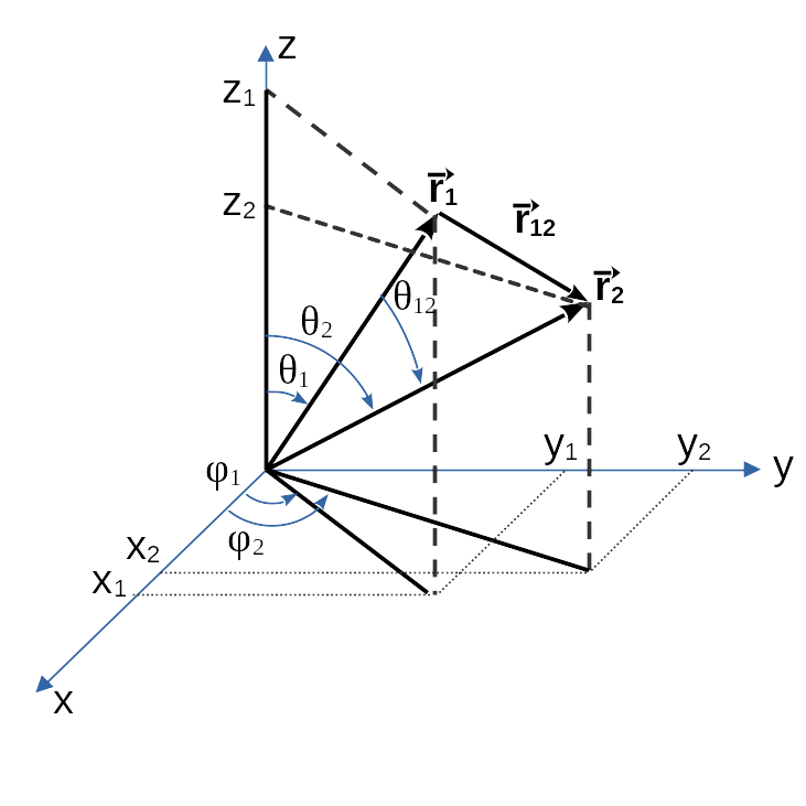
Figure 1: The vectors $\vec{r_{1}}$ and $\vec{r_{2}}$ in the spherical coordinates

It is clear that a direct Taylor expansion of $r_{12}$ or $1/r_{12}$ term, does not converge in the whole space,see Gill [9]. An alternative is an expansion employing the terms $r_{<}^{l}/r_{>}^{(l+1)}\mathit{P_{l}}(\cos{(\theta_{12})})$, where $\mathit{P_{l}}(\cos{(\theta_{12})})$ represents Legendre polynomials [12]. Unfortunatelly this expansion does not converge everywhere, especially at the larger vicinity of singular points.
Now we show an alternative method of expansion of the linear $r_{12}$ function and its Coulombic counterpart $1/r_{12}$ . Let us assign $r_{>}$ and $r_{<}$ to $r_{1}$ and $r_{2}$ in such a way that $r_{>}\geq r_{<}$. We employ the Goldman coordinates [13]

$$u=r_{>},v=\frac{r_{<}}{r_{>}}$$ (6)

Using (6) we can now write

$$r_{12}=u\sqrt{1-2.v.\cos{\theta_{12}}+v^{2}}=u\sqrt{1-2.v.\Big{(}\cos^{2}(\frac{\theta_{12}}{2})-\sin^{2}(\frac{\theta_{12}}{2})\Big{)}+v^{2}}\$$ (7)

Regrouping the terms we obtain the following form

$$r_{12}=u\sqrt{\sin^{2}(\frac{\theta_{12}}{2})(1+v)^{2}+\cos^{2}(\frac{\theta_{12}}{2})(1-v)^{2}}\$$ (8)

Notice that $\sin(\theta_{12}/2)$ and $\cos(\theta_{12}/2)$ are always non-negative in our case since $0\leq\theta_{12}\leq\pi$. Moreover, from (6) immediately follows $0\leq v\leq 1$, which guarantees

$$(1+v)\sin(\frac{\theta_{12}}{2})\geq 0$$ (9)

$$(1-v)\cos(\frac{\theta_{12}}{2})\geq 0.$$ (10)

Now we can define two regions in $(v,\theta_{12})$-coordinate system (see Fig.2)

subspace A

$${(1+v)\sin(\frac{\theta_{12}}{2})}\leq{(1-v)\cos(\frac{\theta_{12}}{2}))}$$ (11)

subspace B elsewhere.

In $(v,\theta_{12})$-coordinates we introduce the functions $X$ and $S$ in the following way:
for the A subspace

$$X=\tan(\frac{\theta_{12}}{2})\Big{(}\frac{1+v}{1-v}\Big{)},$$ (12)

while for the B subspace

$$X=\cot(\frac{\theta_{12}}{2})\Big{(}\frac{1-v}{1+v}\Big{)},$$ (13)

the function $S$ in the A subspace we define as

$$S=u.\cos(\frac{\theta_{12}}{2})(1-v)$$ (14)

while in the B subspace

$$S=u.\sin(\frac{\theta_{12}}{2})(1+v)$$ (15)

It is easy to see that the Coulomb potential can be expressed in both regions A,B in the same way,

$$\frac{1}{r_{12}}=\frac{1}{S\sqrt{1+X^{2}}}$$ (16)

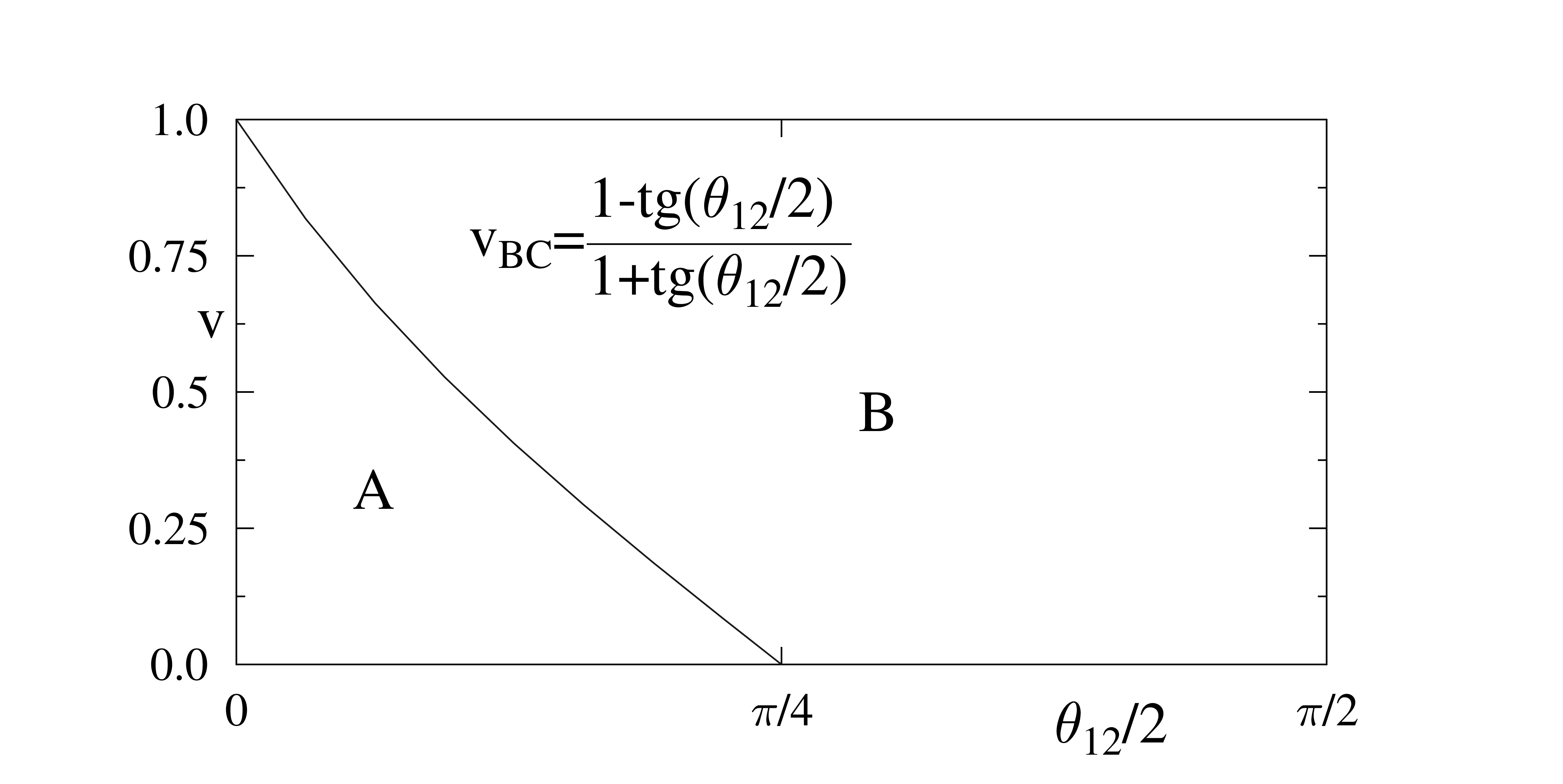
Figure 2: Definition of the subspaces A,B

For the boundary between A and B (Fig.2) follows,

$$v_{BC}=\frac{1-\tan(\frac{\theta_{12}}{2})}{1+\tan(\frac{\theta_{12}}{2})}$$ (17)

On both regions we now have $X\leq 1$. This guarantees the convergence of the Taylor expansion of the functions $\sqrt{1+X^{2}}$ (in the linear term) and $\frac{1}{\sqrt{1+X^{2}}}$ (in the Coulomb potential). Provided $X\leq 1$ these functions can be expanded at the point $X^{2}=X_{c}$:

$$r_{12}=S.\sqrt{1+X^{2}}=S.\Big{(}\sqrt{1+X_{c}}+\frac{1}{2}\frac{(X^{2}-X_{c})}{(1+X_{c})^{\frac{1}{2}}}-\frac{1.1}{2.4}\frac{(X^{2}-X_{c})^{2}}{(1+X_{c})^{\frac{3}{2}}}+$$

$$+\frac{1.1.3}{2.4.6}\frac{(X^{2}-X_{c})^{3}}{(1+X_{c})^{\frac{5}{2}}}-\frac{1.1.3.5}{2.4.6.8}\frac{(X^{2}-X_{c})^{4}}{(1+X_{c})^{\frac{7}{2}}}+\dots\Big{)}$$ (18)

the square root in the denominator can be expanded similarly

$$\frac{1}{r_{12}}=\frac{1}{S.\sqrt{1+X^{2}}}=\frac{1}{S}\Big{(}\frac{1}{\sqrt{1+X_{c}}}-\frac{1}{2}\frac{(X^{2}-X_{c})}{(1+X_{c})^{\frac{3}{2}}}+\frac{1.3}{2.4}\frac{(X^{2}-X_{c})^{2}}{(1+X_{c})^{\frac{5}{2}}}-$$

$$\frac{1.3.5}{2.4.6}\frac{(X^{2}-X_{c})^{3}}{(1+X_{c})^{\frac{7}{2}}}+\frac{1.3.5.7}{2.4.6.8}\frac{(X^{2}-X_{c})^{4}}{(1+X_{c})^{\frac{9}{2}}}-\dots\Big{)}=$$

$$\frac{1}{\sqrt{1+X_{c}}}+\sum_{k=1}^{\infty}(-1)^{k}\frac{(2k-1)!!}{2k!!}\frac{(X^{2}-X_{c})^{k}}{(1+X_{c})^{\frac{2k+1}{2}}}$$ (19)

It is now usefull to define for (18) the coefficients

$$C_{1}=\frac{1}{2},C_{2}=\frac{1.1}{2.4},C_{3}=\frac{1.1.3}{2.4.6},C_{4}=\frac{1.1.3.5}{2.4.6.8},...$$ (20)

(21)

and for (19) the coefficients

$$D_{k}=\frac{(2k-1)!!}{(2k!!)}.$$ (22)

After expansion of the denumerator of $X$ and $S$ we obtaine an expansion of the linear function $r_{12}$ and the Coulomb potential with separate functions of $u$, $v$, and $\theta_{12}/2$. This is the first step of the method. Now we must realize that direct usage of this expansion leads for many particle integrals to almost intractable problems. It is easy to see it from the type of the integrals with our functions $\sin{\frac{\theta_{ij}}{2}}=\sqrt{\frac{1-\cos{\theta_{ij}}}{2}}$ and $\cos{\frac{\theta_{ij}}{2}}=\sqrt{\frac{1+\cos{\theta_{ij}}}{2}}$. The integrations with inclusion of such functions with different combination of angles $\theta_{ij}/2$ lead to large problems, mainly to integrations with combinations of odd powers of our basic goniometric functions. Second, we expanded the goniometric functions with the half-angle argument with the method utilized by author for a long time. In the past author developed a package for expansion of goniometric functions occured in the expansions of the functions $S\sqrt{1+X^{2}}$ and $\frac{1}{S\sqrt{1+X^{2}}}$. It is clear that direct expansion of positive and negative powers of functions $\sin{\frac{\theta_{12}}{2}}=\sqrt{\frac{1-\cos{\theta_{12}}}{2}}$ at the point $\theta_{12}=0$ and in its very near surrounding and simiraly for $\cos{\frac{\theta_{12}}{2}}=\sqrt{\frac{1+\cos{\theta_{12}}}{2}}$ at the point $\theta_{12}=\pi$ leads to large errors in expansion series.
To overcome these problems we propose the following method for expansion of goniometric parts of our expansion of the Coulomb potential and the linear term. First we define new angular coordinates by these two regular transformations (Jacobian of the transformation is non-zero at the whole domain)

$$\theta_{+}=\frac{\theta_{1}+\theta_{2}}{2},\theta_{-}=\frac{\theta_{1}-\theta_{2}}{2}$$ (23)

$$\phi_{+}=\frac{\phi_{1}+\phi_{2}}{2},\phi_{-}=\frac{\phi_{1}-\phi_{2}}{2}.$$ (24)

Fig.3 shows the Domain1 of the regular transformation (23) and the Domain2 of (24), that could be used as subintegration domains. In the Domain1 the y axes belongs to $\theta_{+}/2$ and x axes belongs to $\theta_{-}/2$. Here the border is defined by $\theta_{+}/2$ which is linear function of $\theta_{-}/2$. Similar statements are valid for Domain2 with exchange $\theta\leftrightarrow\phi$.

(a) Domain 1

(b) Domain 2

Figure 3: Domains after regular transformations

It is easy to prove the following identities

$$\sin{\frac{\theta_{12}}{2}}=\sqrt{\sin^{2}(\theta_{-})\cos^{2}(\phi_{-})+\sin^{2}(\theta_{+})\sin^{2}(\phi_{-})}$$ (25)

$$\cos{\frac{\theta_{12}}{2}}=\sqrt{\cos^{2}(\theta_{-})\cos^{2}(\phi_{-})+\cos^{2}(\theta_{+})\sin^{2}(\phi_{-})}.$$ (26)

We can treat equations (25) and (26) in a similar way as we did for 11 for the subspace A and its complement B

$$\rm{Subspace} \rm{C}:|\sin{\theta_{-}}||\cos{\phi_{-}}|\geq|\sin{\theta_{+}}||\sin{\phi_{-}}|$$ (27)

$$\rm{Subspace} \rm{D}:|\sin{\theta_{-}}||\cos{\phi_{-}}|\leq|\sin{\theta_{+}}||\sin{\phi_{-}}|.$$ (28)

It is necessary to underline independence of functions $\cos(\theta_{12})$, $\sin(\theta_{12}/2)$ and $\cos(\theta_{12}/2)$ on the angle $\phi_{+}$, so definition of subspaces does not depend on $\phi_{+}$ either. Upper inequalities define $\phi_{-}$ as two dimensional function, that determines subspaces, where the expansions of the goniometric functions converge

$$|\tan{\phi_{-}}|=\frac{|\sin{\theta_{-}}|}{|\sin{\theta_{+}}|}$$ (29)

Defining $W_{1}$ and $W_{2}$ functions

$$W_{1}=\frac{|\sin{\theta_{+}}|}{|\sin{\theta_{-}}|}|\tan{\phi_{-}}|$$ (31)

$$W_{2}=\frac{|\sin{\theta_{-}}|}{|\sin{\theta_{+}}|}|\cot{\phi_{-}}|$$ (32)

we can rewrite (25) separetely on the subspaces as

$$\rm{Subspace} \rm{C}:\sin{\frac{\theta_{12}}{2}}=|\sin{\theta_{-}}||\cos{\phi_{-}}|\sqrt{1+W_{1}^{2}}$$ (33)

$$\rm{Subspace} \rm{D}:\sin{\frac{\theta_{12}}{2}}=|\sin{\theta_{+}}||\sin{\phi_{-}}|\sqrt{1+W_{2}^{2}}$$ (34)

Analogous manipulations can be done for 26, by changing $\sin{\theta_{-}}$ to $\cos{\theta_{-}}$ and $\sin{\theta_{+}}$ to $\cos{\theta_{+}}$.

$$W_{3}=\frac{|\cos{\theta_{+}}|}{|\cos{\theta_{-}}|}|\tan{\phi_{-}}|$$ (35)

$$W_{4}=\frac{|\cos{\theta_{-}}|}{|\cos{\theta_{+}}|}|\cot{\phi_{-}}|$$ (36)

we can rewrite (25) separetely on the subspaces as

$$\rm{Subspace} \rm{E}:\cos{\frac{\theta_{12}}{2}}=|\cos{\theta_{-}}||\cos{\phi_{-}}|\sqrt{1+W_{3}^{2}}$$ (37)

$$\rm{Subspace} \rm{F}:\cos{\frac{\theta_{12}}{2}}=|\cos{\theta_{+}}||\sin{\phi_{-}}|\sqrt{1+W_{4}^{2}}.$$ (38)

It is necessary to introduce expansions of $X(Space)$ and $1/S(Space)$ (the X and S functions depend on Subspaces A or B)

$$\tilde{X}(A)=\frac{(1+t)}{(1-t)}.R_{sin}.R_{cos^{-1}}$$ (39)

$$\tilde{X}(B)=\frac{(1-t)}{(1+t)}.R_{cos}.R_{sin^{-1}},$$ (40)

$$\frac{1}{\tilde{S}(A)}=\frac{1}{(1-t)}.R_{cos^{-1}}$$ (41)

$$\frac{1}{\tilde{S}(B)}=\frac{1}{(1+t)}.R_{sin^{-1}},$$ (42)

where $R_{sin/cos/sin^{-1}/cos^{-1}}$ are purely goniometric functions, that depend on subspaces C,D,E,F

$$R_{sin}(C)=|\sin{\theta_{-}}||\cos{\phi_{-}}|.(\sqrt{1+W_{1c}}+$$

$$\sum_{l=1}^{N}(-1)^{l+1}C_{l}\frac{(W_{1}^{2}-W_{1c})^{l}}{(1+W_{1c})^{\frac{2l-1}{2}}}),$$ (43)

$$R_{sin}(D)=|\sin{\theta_{+}}||\sin{\phi_{-}}|.(\sqrt{1+W_{2c}}+$$

$$\sum_{l=1}^{N}(-1)^{l+1}C_{l}\frac{(W_{2}^{2}-W_{2c})^{l}}{(1+W_{2c})^{\frac{2l-1}{2}}}),$$ (44)

$$R_{cos}(E)=|\cos{\theta_{-}}||\cos{\phi_{-}}|.(\sqrt{1+W_{3c}}+$$

$$\sum_{l=1}^{N}(-1)^{l+1}C_{l}\frac{(W_{3}^{2}-W_{3c})^{l}}{(1+W_{3c})^{\frac{2l-1}{2}}}),$$ (45)

$$R_{cos}(F)=|\cos{\theta_{+}}||\sin{\phi_{-}}|.(\sqrt{1+W_{4c}}+$$

$$\sum_{l=1}^{N}(-1)^{l+1}C_{l}\frac{(W_{4}^{2}-W_{4c})^{l}}{(1+W_{4c})^{\frac{2l-1}{2}}}),$$ (46)

and for negative powers of $\sin(\theta_{12}/2)$ and $\cos(\theta_{12}/2)$ we have

$$R_{sin^{-1}}(C)=\frac{1}{|\sin{\theta_{-}}||\cos{\phi_{-}}|}.(\frac{1}{\sqrt{1+W_{1c}}}+$$

$$\sum_{l=1}^{N}(-1)^{l}D_{l}\frac{(W_{1}^{2}-W_{1c})^{l}}{(1+W_{1c})^{\frac{2l+1}{2}}}),$$ (47)

$$R_{sin^{-1}}(D)=\frac{1}{|\sin{\theta_{+}}||\sin{\phi_{-}}|}.(\frac{1}{\sqrt{1+W_{2c}}}+$$

$$\sum_{l=1}^{N}(-1)^{l}D_{l}\frac{(W_{2}^{2}-W_{2c})^{l}}{(1+W_{2c})^{\frac{2l+1}{2}}}),$$ (48)

$$R_{cos^{-1}}(E)=\frac{1}{|\cos{\theta_{-}}||\cos{\phi_{-}}|}.(\frac{1}{\sqrt{1+W_{3c}}}+$$

$$\sum_{l=1}^{N}(-1)^{l}D_{l}\frac{(W_{3}^{2}-W_{3c})^{l}}{(1+W_{3c})^{\frac{2l+1}{2}}}),$$ (49)

$$R_{cos^{-1}}(F)=\frac{1}{|\cos{\theta_{+}}||\sin{\phi_{-}}|}.(\frac{1}{\sqrt{1+W_{4c}}}+$$

$$\sum_{l=1}^{N}(-1)^{l}D_{l}\frac{(W_{4}^{2}-W_{4c})^{l}}{(1+W_{4c})^{\frac{2l+1}{2}}}),$$ (50)

A package was written by the author that allows us enumarate Taylor series for both spaces A and B and for positive and negative powers of $\sin(\theta_{12}/2)$ and $\cos(\theta_{12}/2$. Now we can use (18) and (19) with exchange $X\leftrightarrow\tilde{X}$ and $S\leftrightarrow\tilde{S}$ to form final expansions

$$r_{12}\doteq\tilde{S}(\sqrt{1+X_{c}}+\sum_{l=1}^{N}(-1)^{l+1}C_{l}\frac{(\tilde{X}^{2}-X_{c})^{l}}{(1+X_{c})^{\frac{2l-1}{2}}}),$$ (51)

$$\frac{1}{r_{12}}\doteq\frac{1}{\tilde{S}}(\frac{1}{\sqrt{1+X_{c}}}+\sum_{l=1}^{N}(-1)^{l}D_{l}\frac{(\tilde{X}^{2}-X_{c})^{l}}{(1+X_{c})^{\frac{2l+1}{2}}}).$$ (52)

3 Numerical results

To simplify the evaluation of a complete Taylor expansions we define the next function

$$Y^{\pm{1}}\equiv(r_{12}/u)^{\pm{1}}=(\sqrt{1-2v\cos{\theta_{12}}+v^{2}})^{\pm{1}}$$ (54)

We used the averaged absolute differences (AAD) and the normalized averaged absolute differences (NAAD) to statistically assess total Taylor expansion of Coulomb potential and linear term

$$AAD=\frac{1}{N_{\rm{total}}}\sum_{i=1}^{N_{\rm{total}}}|Y^{\pm{1}}_{i}-\tilde{Y}^{\pm{1}}_{i}|$$ (55)

$$NAAD=\frac{1}{N_{\rm{total}}}\sum_{i=1}^{N_{\rm{total}}}\frac{|Y^{-1}_{i}-\tilde{Y}^{-1}_{i}|}{Y^{-1}_{i}}$$ (56)

where $\tilde{Y}^{\pm{1}}$ are expanded $Y^{\pm{1}}$. The sum over $i$-indices means the sum over the individual points of the $v$,$\theta_{1}$,$\theta_{2}$,$\phi_{-}$ space. Step for the $v$ coordinate was $0.01$, for $\theta_{1}$ and $\theta_{2}$ was equal to $\pi/60$ and finally for $\phi_{-}$ was $2\pi/60$. All singular points were excluded from the statistics and the remaining points with finite numerical values were statistically tested. Results are very promising. In the TABLE1 we calculated the AAD and the NAAD parameters for the Coulomb potential and the AAD for $r_{12}$ term. The normalized NAAD parameter could not be calculated for $r_{12}$ due to fact, that this function can reach also a zero values. In the TABLE2 we focus on the region near the singularities. The $v$ coordinate ranges from $0.9$ to $0.99999999999$ with increment $9\times 10^{-k}$, where $k=2,..,10$ and angles $\theta_{-}$($\theta_{-}=\theta_{1}-\theta_{2}$) and $\phi_{-}$ from $10^{-1}$,$10^{-2}$, etc. to $10^{-15}$. The AAD and NAAD were calculated by averaging over $\theta_{1}$ angles chosen from the interval $\theta_{1}\in\langle 0,\pi\rangle$ with the step $\delta=\pi/30$ , see TABLE2. Results are remarkably precise.

Table 1: Statistical parameters AAD (55) and NAAD (56) for $1/r_{12}$ and $r_{12}$

TAB1	AAD		NAAD
Series count	N=7	N=10	N=7	N=10
$1/r_{12}$	$1.58387059E-04$	$8.59742086E-06$	$1.70226807E-04$	$9.32504058E-06$
$r_{12}$	$2.31911797E-05$	$1.04832261E-06$	$-$	$-$
Series count	N=20	N=30	N=20	N=30
$1/r_{12}$	$7.10235347E-10$	$7.17956100E-14$	$7.82848163E-10$	$7.97365766E-14$
$r_{12}$	$6.63828690E-11$	$6.04972850E-15$	$-$	$-$

Table 2: AAD and NAAD near vicinity of singularities and cusp region
AAD and NAAD were averaged through 31 angles $\theta_{1}\in\langle 0,\pi\rangle$

TAB2	AAD	NAAD
Series count	N=30	N=30
$1/r_{12}$	$6.20562199E-05$	$2.63539895E-13$
$r_{12}$	$1.02031516E-16$	$-$

4 Discussion

The advantage of the new expansion of the Coulomb potential and the linear $r_{12}$ function is their accuracy, results are close to the exact potential also near singularities and close to the exact values of the linear term near cusp points. Its disadvantage is the complexity of the method. The author found also other methods of expansion of the potential, but the method shown in this article seems to us to be the most promising. Future work will be focused on a creation of the integral package for calculations of the integrals, which are necessary for quantum problems in the case, where our method for expansion of the Coulomb potential will be used.

5 Acknowledgement

The author is deeply indebted to Jiří Pittner for help with preparing the manuscript and for important valuable discussions of mathematical aspect of the problem. The autor is grateful for consultation the mathematical problems also to Ilja Martišovitš and Roman Čurík. Special thanks are due to Štefan Varga for his valuable comments on the article, previous version of the method and for its numerical testing. Author is very grateful
to Štefan Dobiš for technical support and to Michal Kopčok for preparing a figures for the article.
I would like to express many thanks to my doctor Lucia Mikulášová, without her care our work would not be finished. This work is dedicated to the memory of my father Ján Habrovský.
Our research was supported by the grant GACR 19-01897S.

References

[1]
E.A. Hylleraas, Über den grundzustand des heliumatoms, Z. Phys. 48, 469 (1928)
[2]
E.A. Hylleraas, Neue Berechnung der energie des heliums im grundzustande,sowie des terms von ortho-helium, Z. Phys. 54, 347 (1929)
[3]
R. Habrovský, An explicitly correlated helium wave function in hyperspherical coordinates, Chem. Phys. Lett. 698, 120 (2018)
[4]
A.A. Frost, The Use of Interparticle Coordinates in Electronic Energy Calculations for Atom and Molecules, Theoret. chim. Acta 1, 36 (1962)
[5]
J. Noga,W. Kloper and W.Kutzelnigg, CC-R12: An Explicitly Correlated Coupled-Cluster Theory, Recet Advances in Coupled-Cluster Methods,
I. Recent Advances in Computational Chemistry: Volume 3 (1997)
[6]
S. Ten-no,J. Noga, Explicitly correlated electronic structure theory from R12/F12 ansätze, Wiley Interdisciplinary Reviews,2, 114 (2011)
[7]
S. Kedžuch, O. Demel, J. Pittner, S. Ten-no, Multireference F12 coupld cluster theory. The Brillouin-Wigner approach with single and
double excitations, 511, 418 (2021)
[8]
O. Demel, M.J. Lecours, R. Habrovský, M. Nooijen, Towards Laplace MP2 method using range separated Coulomb potential and orbital selective virtuals,
J.Chem.Phys., 155, 154104 (2021)
[9]
P.M.W. Gill, A new expansion of the Coulomb interaction, Chem. Phys. Lett. 270, 193 (1997)
[10]
H.S. Cohl, A.R.P. Rau, J.E. Tohline, D.A. Browne, J. E. Cazes, E.I. Barnes, Useful alternative to the multipole expansion of 1/r potentials, Phys. Rev. A,
64, 052509 (2001)
[11]
J.G. Ángyán, I. Gerber, M. Marsman, Spherical harmonic expansion of short-range screened Coulomb interactions, J. Phys, A: Math. Gen. 39, 8613 (2006)
[12]
H.A. Bethe and E.E. Salpeter, Quantum mechanics of one- and
two-electron atoms, (Springer-Verlag 1952)
[13]
S.P. Goldman, Uncoupling correlated calculations in atomic physics: Very high accuracy and easy, Phys. Rev. A 57, 677 (1998)