Separability criterion using one observable for special states: Entanglement detection via quantum quench

Abstract

Detecting entanglement in many-body quantum systems is crucial but challenging, typically requiring multiple measurements. Here, we establish the class of states where measuring connected correlations in just one basis is sufficient and necessary to detect bipartite separability, provided the appropriate basis and observables are chosen. This methodology leverages prior information about the state, which, although insufficient to reveal the complete state or its entanglement, enables our one basis approach to be effective. We discuss the possibility of one observable entanglement detection in a variety of systems, including those without conserved charges, such as the Transverse Ising model, reaching the appropriate basis via quantum quench. This provides a much simpler pathway of detection than previous works. It also shows improved sensitivity from Pearson Correlation detection techniques.

Introduction:

Detection of many-body entanglement (bi-partite or multipartite) is an experimentally difficult task. So far only a handful of experiments [1, 2] have been able to successfully achieve it. The set-up of Ref. [1] uses a replica of the original many-body system to compute purity. On the other hand, Ref. [2] use a series of randomized measurements to detect entanglement in trapped ion quantum simulator. Both these set-ups are fine tuned and while they can measure the entanglement of a carefully prepared state in an idealized setting, measuring or witnessing entanglement of states obtained in many-body experiments simply and effectively is practically impossible[3].

Hence it is of paramount importance to connect entanglement detection in specific classes many-body states with quantities requiring less demanding experimental resources to measure. The definition of an entangled state is one that cannot be separated into individual states belonging in separate subspaces. In the case of a bipartite system with constituent Hilbert spaces $\mathcal{H}_{A}$ and $\mathcal{H}_{B}$, the combined space is given by $\mathcal{H}=\mathcal{H}_{A}\otimes\mathcal{H}_{B}$, and a pure state $|\psi\rangle\in\mathcal{H}$ is separable iff,

$$|\psi\rangle=|\psi_{A}\rangle\otimes|\psi_{B}\rangle$$ (1)

where $|\psi_{A[B]}\rangle\in\mathcal{H}_{A[B]}$. On the other hand, a mixed state represented by $\rho$ is separable iff

$$\rho=\sum_{i}p_{i}\rho_{i}^{A}\otimes\rho_{i}^{B}$$ (2)

where $\rho_{i}^{A[B]}\in\mathcal{H}_{A[B]}$ and $\sum_{i}p_{i}=1$.

Entanglement indicates quantum correlations, and measurement of classical correlations between one set of observables between the corresponding subsystems is typically not enough to detect entanglement — classical correlations should necessarily exist in all measurements. The search for detection of entanglement with least number of measurements have taken us in various directions in recent years[4, 5, 6, 7, 8, 9, 10], with specific techniques available for spin systems[11, 12, 13, 14, 15, 16], measuring charge fluctuations [17, 18, 19, 20], coherences [21] or number entropy[22, 23, 24, 25] in systems with locally conserved charge, and measurements of classical correlations in a set of Mutually Unbiased Bases(MUBs) or observables[26, 27, 28, 29, 30, 31].

In this work we shall focus on detection of bipartite entanglement efficiently. Previous studies involving MUBs have revealed that at least two measurements are necessary to establish a reliable criterion for detection. However, considering that bipartite entanglement typically implies classical correlation in all measurements, for separable states, there should exist at least one measurement that exhibits zero correlation. Then by measuring this specific quantity, our problem of entanglement detection should be resolved. But the challenge lies in the fact that there is no guarantee of existence of such a quantity that is independent of the state being examined, thus leading to a wide variety of state-dependent entanglement witnesses.

In this work we find a common observable which can efficiently detect bipartite entanglement for a wide class of states. We demonstrate that, (i) it is in fact possible to detect separability of any arbitrary mixed state via measuring correlations of one observable independently of the measured state, if they are separable to purely real or imaginary states. (ii) We also show that in presence of a locally conserved charge such as particle number/magnetization, detection of entanglement in any generic state (i.e. need not be separable to purely real or imaginary) is possible by this technique. (iii) We then test the efficacy of the observable to detect entanglement in mixed states generated by different Hamiltonians via exact numerical simulations.

In what follows, since our proposed criterion will be based on a MUB, we first define what is a MUB and discuss a specific entanglement witness which utilizes them. Then we elaborate our criterion and provide examples comparing efficiency of both approaches.

Mutually Unbiased Basis(MUB):

A set of mutually unbiased basis $\{\bm{\alpha}\}=\{\ket{\alpha_{i}}\}$ and $\{\bm{\alpha^{\prime}}\}=\{\ket{\alpha^{\prime}_{j}}\}$ where $i,j\in 1,\ldots,d$, for a Hilbert space $\mathcal{H}=\mathbb{C}^{d}$ is defined by the relation,

$$|\langle\alpha_{i}|\alpha^{\prime}_{j}\rangle|^{2}=1/d\hskip 36.135pt\forall\hskip 14.45377pti,j$$ (3)

Entanglement witnessing using MUBs

Entanglement detection using MUBs requires measurement of correlations. Among several different quantifiers addressed in previous works [26, 27, 28, 29, 30, 31], we focus on the Pearson correlation measurement, as it was shown to be among the more efficient measures.[28]

Consider a system $S$, divided into two subsystems $A$ and $B$. Let us denote an observable measured in subsystem $A$ as $\mathcal{O}_{A}$ and for $B$ as $\mathcal{O}_{B}$. Then the Pearson correlation between the observables is given by the normalized connected correlation,

$$\mathcal{P}_{\mathcal{O}}=\frac{\langle\mathcal{O}_{A}\otimes\mathcal{O}_{B}\rangle-\langle\mathcal{O}_{A}\otimes\mathbb{I}\rangle\langle\mathbb{I}\otimes\mathcal{O}_{B}\rangle}{\sqrt{\langle\mathcal{O}_{A}^{2}\otimes\mathbb{I}\rangle-\langle\mathcal{O}_{A}\otimes\mathbb{I}\rangle^{2}}\sqrt{\langle\mathbb{I}\otimes\mathcal{O}_{B}^{2}\rangle-\langle\mathbb{I}\otimes\mathcal{O}_{B}\rangle^{2}}},$$ (4)

where the expectation value is taken with respect to the state of the system $S$. For MUB measurement, we assume the set of eigenvectors for $\mathcal{O}_{A}$ as$\{\ket{\alpha}\}$, then we can find another observable $\mathcal{O}^{\prime}_{A}$ with eigenvectors $\{\ket{\alpha^{\prime}}\}$ fulfilling Eq. 3. Similar construction can be done for subsystem $B$. Then

$$|\mathcal{P}_{\mathcal{O}}|+|\mathcal{P}_{\mathcal{O}^{\prime}}|>1$$ (5)

is a sufficient but not necessary condition for the two halves of the system to be entangled [28]. Further improvements on the bound were provided by measuring correlations in more than two MUBs.

Hereafter, we shall establish the case where measurements in two basis are not needed, i.e., non-zero connected correlations in one basis immediately indicates entanglement.

One measurement entanglement detection:

For completeness we discuss the cases of both pure and mixed states,

1. Pure states: In the study of many-body physics we often work with pure states, when we isolate the experimental set-up from interactions with the environment. In this case,

   $$\mathcal{C}_{1}=\langle\mathcal{O}_{A}\otimes\mathcal{O}_{B}\rangle-\langle\mathcal{O}_{A}\otimes\mathbb{I}\rangle\langle\mathbb{I}\otimes\mathcal{O}_{B}\rangle$$ (6)

   $=0$, is a necessary and sufficient condition for zero entanglement between the partitions. $\mathcal{O}_{A}$ and $\mathcal{O}_{B}$ should be chosen so as to give non-zero expectation values.

   The proof directly follows from Eq. (1).

2. Mixed states: For generic mixed states, $\mathcal{C}_{1}=0$ is still a sufficient but not a necessary condition for separability. To illustrate this, consider a separable state $\rho_{CC}$ given by,

   $$\rho_{CC}=\frac{1}{d}\sum_{i=1}^{d}\ket{\alpha_{i}}\bra{\alpha_{i}}\otimes\ket{\beta_{i}}\bra{\beta_{i}}$$ (7)

   where $\{|\beta\rangle\}$ is the eigenbasis of $\mathcal{O}_{B}$. In this case, $\mathcal{C}_{1}$ can show high correlations, but

   $$\mathcal{C}_{2}=\langle\mathcal{O}^{\prime}_{A}\otimes\mathcal{O}^{\prime}_{B}\rangle-\langle\mathcal{O}^{\prime}_{A}\otimes\mathbb{I}\rangle\langle\mathbb{I}\otimes\mathcal{O}^{\prime}_{B}\rangle$$ (8)

   will be equal to $0$.

   For the generic separable mixed state of Eq. (2) correlations may exist in multiple bases, but there is no entanglement present. This can be seen by choosing appropriate $\mathcal{O}_{A}$ and $\mathcal{O}_{B}$ to compute,

   $$\langle\mathcal{O}_{A}\otimes\mathcal{O}_{B}\rangle =\sum_{i}p_{i}{\rm Tr}[\rho_{i}^{A}\mathcal{O}_{A}]{\rm Tr}[\rho_{i}^{b}\mathcal{O}_{b}]$$

   $$\langle\mathcal{O}_{A}\otimes\mathbb{I}\rangle\langle\mathbb{I}\otimes\mathcal{O}_{B}\rangle =\sum_{i}p_{i}{\rm Tr}[\rho_{i}^{A}\mathcal{O}_{A}]\sum_{j}p_{j}{\rm Tr}[\rho_{j}^{b}\mathcal{O}_{b}]$$ (9)

   If $p_{i}=1$, i.e., the system is separable to $\rho=\rho^{A}\otimes\rho^{B}$, then $\mathcal{C}_{1}=\mathcal{C}_{2}=0$, and the condition becomes necessary. For all other typical cases it is not. Thus, entanglement witness bounds usually involve computation of correlations in several measurements.

To overcome this difficulty, we attempt to construct a common observable for all density matrices whose measurement shall also provide the necessary criterion. As mentioned before, a common observable is not guaranteed to exist for arbitrary density matrices, so we search for classes of states which allow us to do so.

Construction of the observable:

Let us consider the case of L-qubits, i.e. Hilbert spaces of dimension $2^{L}$ and relegate the generalization to qudits to Appendix B. From the previous discussion of $\rho_{CC}$, choosing an observable whose eigenbasis is mutually unbiased to $\{|\alpha\rangle,|\beta\rangle\}$, which we label as the $\sigma_{z}$ (computational) basis of the respective systems is clearly necessary. Additionally, for separable states not of the form of $\rho_{CC}$, any arbitrary mutually unbiased observable does not yield $\mathcal{C}_{2}=0$. Ideally since we also want a basis easily implementable in experiments, the special observable should to be realized by very local (involving on-site or nearest neighbour) transformations. While this is not easily realizable for qudits of arbitrary dimensions, in the L-qubit scenario, a special observable whose eigenbasis is mutually unbiased to the computational basis can be created by rotating $\mathcal{O}_{A[B]}$ via

$$U_{A[B]}=(e^{-i\sigma^{x}\pi/4})^{\otimes L_{A[B]}},$$ (10)

where $L_{A[B]}$ is the length of subsystem $A[B],L_{A}+L_{B}=L$.

By explicit construction (see Appendix A), we see $U$ has the following properties.

1. $U_{A[B]}^{T}=U_{A[B]}$.
   

2. $(U_{A[B]})_{p,q}(U_{A[B]})_{d-p+1,q}=\frac{1}{L_{A[B]}}e^{-i\pi L_{A[B]}/2}$ and
   

3. $(U_{A[B]})_{p,q}=\frac{1}{\sqrt{L_{A[B]}}}e^{-i\pi(\phi_{p,q})/2}$, where $\phi_{p,q}\in[0,L_{A[B]}]\cap\mathbb{Z}$

Moving to the Schroedinger picture and henceforth dropping the subscript $i$ for brevity, we obtain the density matrix after the evolution,

$$\rho^{\prime}_{i_{A},i_{B},j_{A},j_{B}}=(U_{A}\otimes U_{B})_{i_{A},i_{B},k_{A},k_{B}}\rho_{k_{A},k_{B},l_{A},l_{B}}(U_{A}\otimes U_{B})^{\dagger}_{l_{A},l_{B},j_{A},j_{B}}$$ (11)

We see that the connected correlator with respect to $\rho^{\prime}$ is identically $0$, when the following conditions are fulfilled,

1. $\rho$ is separable to purely real [imaginary] density matrices, i.e. $\rho_{A[B]}\in\mathbb{R}^{d_{A[B]}\times d_{A[B]}}[i\mathbb{R}^{d_{A[B]}\times d_{A[B]}}]$.

2. The observable $\mathcal{O}$ is chosen to be diagonal in the computational basis with eigenvalues $E_{j}=\{f(j)+c_{1}\ni f(j)=-[+]f(d-j+1),j\in[1,d]\cap\mathbb{Z},c_{1}\in\mathbb{R}\}$. Examples of such observables include total particle number or total magnetization in many-body systems, or the $S_{z}$ index in large spin systems, all typically measurable by local measurements. The ‘$[+]$’ is required for imaginary case of the previous condition.

OR

$\rho$ is separable, the state has a locally conserved charge, such as magnetization or particle number, and we perform subsystem measurements of the conserved charge.

We first show our conjecture is valid when the first two conditions are fulfilled. We see that,

$$\begin{split}&{\rm Tr}[\rho^{\prime A}\mathcal{O}_{A}]=\frac{1}{d}\sum_{p=1}^{d/2}\sum_{q,r}^{d}(f(p)+c_{1})(U_{A})_{p,q}\rho_{qr}(U_{A})^{*}_{r,p}\\ &+\frac{1}{d}\sum_{p=1}^{d/2}\sum_{q,r}^{d}(-f(p)+c_{1})(U_{A})_{d-p+1,q}\rho_{q,r}(U_{A})^{*}_{r,d-p+1}\end{split}$$ (12)

Then using the properties of $U_{A}$ we can simplify Eq. 12 by realizing that,

$$\sum_{p=1}^{d/2}\sum_{q,r}^{d}f(p)(U_{A})_{d-p+1,q}\rho_{q,r}(U_{A}^{*})_{r,d-p+1}$$

$$=\sum_{p=1}^{d/2}\sum_{q,r}^{d}f(p)e^{-i\pi/2(\phi_{p,q}-\phi_{r,p})}\rho_{q,r}$$

$$=\sum_{p=1}^{d/2}\sum_{q,r}^{d}f(p)e^{-i\pi/2[(L_{A}-\phi_{p,q})-(L_{A}-\phi_{r,p})]}\rho_{q,r}$$

$$=\sum_{p=1}^{d/2}\sum_{q,r}^{d}f(p)(U_{A})_{p,q}\rho_{q,r}(U_{A}^{*})_{r,p}$$ (13)

where in the third step, we have used $U_{A}^{T}=U_{A}$ and $\rho_{q,r}=\rho_{r,q}$, for purely real $\rho_{A}$. For purely imaginary $\rho_{A}$, we shall have $\rho_{q,r}=-\rho_{r,q}$, hence we need to choose $f(j)=f(d-j+1)$. Then Eq. 12 immediately simplifies to yield

$${\rm Tr}[\rho^{\prime A}\mathcal{O}_{A}] = \frac{1}{d}\sum_{p=1}^{d}\sum_{q,r}^{d}c_{1}(U_{A})_{p,q}\rho_{q,r}(U_{A})^{*}_{r,p}$$ (14)

$$=c_{1}{\rm Tr}[\rho^{\prime A}]=c_{1}$$

Thus we have proven that for any real [imaginary] density matrix $\langle\mathcal{O}^{\prime}_{A}\otimes\mathbb{I}\rangle$ gives a constant value, $c_{1}$ depending on parameters of the operator chosen. Applying this to $\langle\mathbb{I}\otimes\mathcal{O}^{\prime}_{B}\rangle$ and $\langle\mathcal{O}^{\prime}_{A}\otimes\mathcal{O}^{\prime}_{B}\rangle$ and utilizing $\rho=\sum_{i}p_{i}\rho_{i}^{A}\otimes\rho_{i}^{B}$ we also obtain constant values say, $c_{2}$, and $c_{1}c_{2}$ respectively. Now the connected correlator becomes

$$\langle\mathcal{O}^{\prime}_{A}\otimes\mathcal{O}^{\prime}_{B}\rangle-\langle\mathcal{O}^{\prime}_{A}\otimes\mathbb{I}\rangle\langle\mathbb{I}\otimes\mathcal{O}^{\prime}_{B}\rangle$$ (15)

$$= \sum_{i=1}^{d}p_{i}c_{1}c_{2}-(\sum_{i=1}^{d}p_{i}c_{1})(\sum_{j=1}^{d}p_{j}c_{2})$$

$$= 0$$

Eq. 15 thus defines a sufficient condition for separability which becomes necessary when the two conditions are fulfilled. Hence,
For any set of states separable to purely real [or purely imaginary] states, a single measurement of the connected correlation in special MUBs is sufficient to detect entanglement.

Note that this result is stable against small perturbations to the first condition, i.e. if we add imaginary separable states of strength $O(\epsilon)$ to a real separable states, Eq. (14) is weakly upper bounded by $(1+O(\epsilon))c_{1}+O(\epsilon)|f(j)|_{{\rm max}}$, which indicates corrections are perturbative for bounded $\mathcal{O}_{A}$.

The unitary transformation $U_{A}$ is not unique, but it is also not an arbitrary MUB to the computational basis. In Appendix B, we provide another explicit example of $U_{A}$, although it is not as local as the current example, but has the advantage of working for a collection of qudits. Further note that if we were able to obtain $U_{A[B]}$ of the above form but with the additional property,

$$\phi_{p,q}-\phi_{p,r}=2m,\hskip 14.45377ptm\in\mathbb{Z}$$ (16)

this technique would be applicable without the first condition. Unfortunately, this renders the matrix non-unitary and thus is an invalid choice. However with conserved local magnetization (the alternative condition), only specific elements of $U_{A}$ are responsible for the rotation. In this set-up, Eq. (16) is fulfilled, leading to applicability for generic density matrices. See Appendix C for details. Nonetheless, an intuitive argument exists for the alternative condition for applicability to generic density matrices which we describe below.

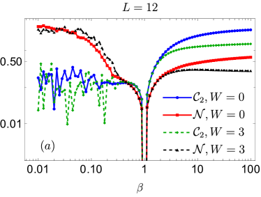
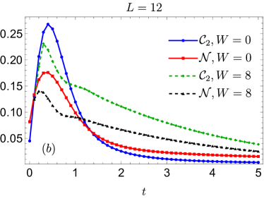
Figure 1: Comparison of behaviour of $\mathcal{C}_{2}$ [Eq. (8)] with $\mathcal{N}$ [Eq. (21)] for top: different values of $\beta$ for states defined in Eq. (19) of the model defined in Eq. (18) for two different $W$ and bottom: for dissipative evolution via Eq. (20) starting from Néel state. $\mathcal{O}_{A}=\sum_{i=1}^{L_{A}}\sigma^{z}_{i}$ and $\mathcal{O}_{B}=\sum_{i=L_{A}+1}^{L_{B}}\sigma^{z}_{i}$, $U_{A[B]}$ is given by Eq. (10)

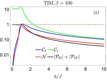
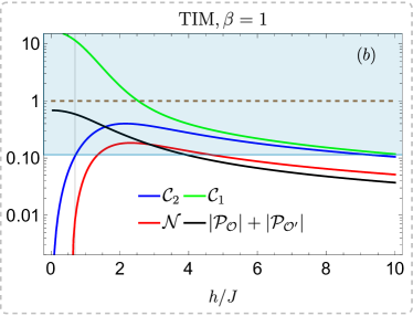
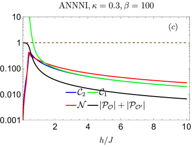
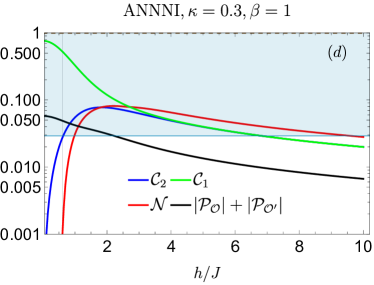
Figure 2: Comparison of behaviour of $\mathcal{C}_{1}$ and $\mathcal{C}_{2}$ defined in Eqs. (6),(8), to $\mathcal{N}$[Eq. (21)] and the criterion in Eq. (5) for the model given in Eq. (22), for(a) $\kappa=0$ at $\beta=1/T=100$, (b) $\kappa=0$ at $\beta=1$, (c) $\kappa=0.3$ at $\beta=100$ and (d) $\kappa=0.3$ at $\beta=1$. The system size is $L=12$, the blue shaded region in (b) and (d) shows the region where $\mathcal{C}_{2}$ is above the cut-off and entanglement detection is possible. The brown dashed line denotes the cut-off $1$ above with entanglement detection is possible via Eq. (5). A small longitudinal field of strength $10^{-3}$ is added to break degeneracy.

We borrow the result from Eq. (5) and choose $\mathcal{O}_{A[B]}$ to be the conserved local charge, say for example the magnetization. Since this implies $\sum_{i=1}^{L_{A}}\langle\sigma^{z}_{i}\rangle+\sum_{i=L_{A}+1}^{L_{B}}\langle\sigma^{z}_{i}\rangle=M$, then by choosing $\mathcal{O_{A}}=\sum_{i=1}^{L_{A}}\sigma^{z}_{i}$ and $\mathcal{O_{B}}=\sum_{i=L_{A}+1}^{L_{B}}\sigma^{z}_{i}$, $|\mathcal{P}_{\mathcal{O}}|=1$ as the two observables are always completely linearly correlated. This reduces Eq. (5) to,

$$|\mathcal{P}_{\mathcal{O^{\prime}}}|>0$$ (17)

Hence any connected correlation in any MUB to the computational basis will indicate entanglement . Since the unitary evolution in Eq. (10) generates such a basis, we shall be able to detect entanglement between $A$ and $B$ by measuring correlation between the total magnetization of the subsystems after the evolution. Thus we have,

In presence of a locally conserved charge, a single measurement of connected correlation in specific MUBs is sufficient to detect entanglement for arbitrary states.

For an arbitrary state where we have no prior knowledge, our test indicates whether it can be separated to completely real (or imaginary) states. This technique then serves as a complement to other entanglement witness techniques which focus on entanglement detection, by identifying the complementary—a large class of separable states. However typically when we generate a state we do have some prior information about it. Hence to test the efficacy of this technique in experimentally detecting entanglement of mixed states generated by generic Hamiltonians, we numerically compare $\mathcal{C}_{2}$ with a quantity originating from the PPT criterion[36, 37], entanglement negativity $\mathcal{N}$. We provide two examples below, (i) Heisenberg models, which conserves magnetization, (ii) Ising models, which do not conserve magnetization. A third example of PXP model, a constrained model which does not conserve magnetization, is provided in Appendix E. We shall see that while for the Heisenberg model it immediately detects entanglement, for the Ising models, additional information about the state is needed to detect entanglement.

Example I— Heisenberg model with quasi periodic disorder

The Heisenberg model with on-site quasiperiodic disorder is described by the following Hamiltonian[38],

$$H=-J\sum_{k}\bm{\sigma}_{k}\cdot\bm{\sigma}_{k+1}+\sum_{k}h_{k}\sigma_{k}^{z}.$$ (18)

In this equation, $\bm{\sigma}=(\sigma^{x},\sigma^{y},\sigma^{z})$ represents a vector of Pauli matrices. The term $h_{k}$ is the quasiperiodic component given by $h_{k}=W\cos(2\pi\eta k)$, where $\eta=\frac{\sqrt{5}-1}{2}$ and $W$ represents the strength of the disorder. We take $J=1$. The inclusion of the quasiperiodic term allows for the study of a more general model, while eliminating the need for averaging over realizations that would be required with random disorder.

We consider computing the entanglement in the following two cases, (i)for the equilibrium density matrix at any temperature $T=1/\beta$, given by the Gibbs state,

$$\rho=\sum_{i=1}^{d^{2}}\frac{e^{-\beta\epsilon_{i}}}{\sum_{i=1}^{d^{2}}e^{-\beta\epsilon_{i}}}\ket{E_{i}}\bra{E_{i}}$$ (19)

where $\epsilon_{i}$ denotes the eigenenergies and $\ket{E_{i}}$ denotes the corresponding eigenvectors; (ii)a time evolution in an open quantum system where the unitary evolution is governed via the Hamiltonian in Eq. (18) and the influence of the environment is effectively included via the Lindblad equation of motion [39]:

$$\frac{d\rho}{dt}=i[H,\rho]+\sum_{k}([L_{k}\rho,L_{k}^{\dagger}]+[L_{k},\rho L_{k}^{\dagger}]),$$ (20)

where $\rho$ represents the density matrix describing the system, and $H$ is the Hamiltonian from Eq. (18). The Lindblad operators $L_{k}$ capture the interactions between the system and the environment. We consider only on-site dephasing term of strength $\gamma$, $L_{k}=\sqrt{\frac{\gamma}{2}}\sigma^{z}_{k}$, which causes the system to eventually evolve to maximally mixed states, to ensure conservation of magnetization, and choose the initial state to be the Néel state[40, 41]. We select these specific cases in order to examine and analyse mixed states, thereby avoiding the trivial scenario of pure state entanglement detection. We restrict our system in the $\sum_{k=1}^{L}\sigma^{z}_{k}=0$ sector.

In Fig.1(a), we present the results for case (i). Notably, $\mathcal{C}_{2}$ (Eq.(8)) with observables $\mathcal{O}_{A[B]}=\sum_{i=1}^{L_{A[B]}}\sigma^{z}_{i}$, and unitary transformations $U_{A[B]}$ [Eq.(10)], successfully detects entanglement in the same parameter regimes where the entanglement measure $\mathcal{N}$, defined as

$$\mathcal{N}=\frac{||\rho^{\Gamma_{A}}||_{1}-1}{2},$$ (21)

is greater than $0$. Here, $\rho^{\Gamma_{A}}$ represents the partial transpose with respect to subsystem $A$, and $||X||_{1}$ denotes the trace norm of operator $X$. This correspondence demonstrates that our criterion of non-zero $\mathcal{C}_{2}$ aligns with the violation of the positive partial transpose (PPT) criterion for both instances of disorder considered. Additionally, it is worth noting that $\mathcal{C}_{2}$ exhibits a value of $0$ at $\beta=1$, consistent with separability according to the PPT criterion. Moreover, the qualitative agreement between $\mathcal{C}_{2}$ and $\mathcal{N}$ becomes more pronounced at higher $\beta$ values, corresponding to purer states.

In Fig. 1(b), where we examine case (ii), there is no separability during the time evolution. However, $\mathcal{C}_{2}$ exhibits the ‘entanglement barrier’ feature previously observed in other measures of entanglement and also in $\mathcal{N}$ [42]. For larger disorder, we observe that the barrier shifts to lower time-scales due to the earlier decay of long-range correlations in such systems [43]. Thus, the measurement of $\mathcal{C}_{2}$ provides a reliable technique to detect entanglement in such systems. It is worth noting that in the presence of locally conserved charge, one can adjust the quench procedure to suit the experiment as long as an observable is generated whose eigenbasis is mutually unbiased with respect to the computational basis.

Example II— Anisotropic next-nearest neighbour Transverse Ising model:

Next, consider the model Hamiltonian,

$$H=-J\sum_{k}\sigma^{z}_{k}\sigma^{z}_{k+1}+\kappa\sum_{k}\sigma^{z}_{k}\sigma^{z}_{k+2}-h\sum_{k}\sigma^{x}_{k}$$ (22)

This is the non-integrable anisotropic next-nearest neighbour Transverse Ising (ANNNI) model, which reduces to the integrable Transverse Ising (TI) model when $\kappa=0$. Note that this model does not have a simple locally conserved charge such as magnetization, so quantities such as number entropy or particle fluctuations cannot detect entanglement.

In the limit of $\beta\rightarrow\infty$, the Transverse Ising (TI) model undergoes a second-order phase transition at $h=h_{c}=1$ for $L\rightarrow\infty$. This phase transition is also observed in the anisotropic next-nearest neighbour Transverse Ising (ANNNI) model, but within a limited parameter range. As we gradually increase the parameter $\kappa$ in the ANNNI model, the critical value of $h$ decreases, and at $\kappa=0.5$, the critical value becomes $h_{c}=0$. [44, 45, 46]. Once again, we investigate the behaviour of $\mathcal{C}_{2}$ in comparison to $\mathcal{N}$ in the thermal states of the models described by the ANNNI Hamiltonian. The thermal states are given by Eq. (19), but with the Hamiltonian $H$ now specified by the ANNNI model.

From Fig. 2, it is evident that in all scenarios, the behaviour of $\mathcal{C}_{2}$ for the same observables as before is qualitatively similar to that of the entanglement measure $\mathcal{N}$. However, the agreement of $\mathcal{C}_{1}$ is dependent on the chosen parameters. Furthermore, the criteria in Eq. (5), $|\mathcal{P}_{\mathcal{O}}|+|\mathcal{P}_{\mathcal{O}}^{\prime}|>1$, denoted by the brown dashed line, is not fulfilled almost everywhere, thus being a poor entanglement witness in this set-up. An improvement could potentially be achieved by increasing the number of mutually unbiased basis (MUB) measurements, although the analysis of this is beyond the scope of the present study. However, a complete agreement between $\mathcal{C}_{2}$ and $\mathcal{N}$ for all values of $h$ with $\kappa=0$ and $\kappa=0.3$ only occurs at large values of $\beta$, where the state becomes minimally mixed.

For smaller $\beta$, there is a region where $\mathcal{N}=0$ while $\mathcal{C}_{2}$ has a small value. Here the system is separable via PPT criterion, but not to purely real states (or there exists bound entanglement). However there still exists a qualitative similarity of $\mathcal{C}_{2}$ with $\mathcal{N}$, which is due to the stability of the correlator to perturbation with imaginary separable states. We can utilize this qualitative similarity to define a lower non-zero cut-off of $\mathcal{C}_{2}$ at each $\beta$ which can be used to detect entanglement. The cut-off can be found using numerical simulations for small size systems and extrapolated to larger sizes, due to weak dependence on system size (See Appendix D) and thus provides a viable route to detect entanglement of states at thermal equilibrium. Note that an arbitrary MUB to computational basis does not yield qualitatively similar results to $\mathcal{N}$ in this case unlike the previous one.

The experimental realization of the Transverse Ising model is possible, for example, in quantum wires by tuning the chemical potential appropriately. [48]. After letting the system reach thermal equilibrium, to perform the rotation one would need perform a quench by ‘pinching’ between neighbouring electrons to ensure $J=\kappa=0$ and let the system evolve for time $t=\frac{\pi}{4h}+2k\pi$,for $k\in\mathbb{Z}$ and measure the total $\sigma_{z}$ correlations between the corresponding parts of the system. Then by using the thresholds for the specific temperature, we can detect entanglement.

Conclusion:

In this work, we have showcased how measuring the one-connected correlation in the appropriate basis can provide valuable insights into the separability of the state and effectively detect entanglement by leveraging specific properties of the state. This approach offers a substantial reduction in the experimental burden for a wide range of systems, as compared to previous correlation measurement methods that often require multiple basis measurements to achieve efficient detection. Moreover, our method presents an alternative means of detecting entanglement in charge-conserved systems.

We have demonstrated the immediate applicability of our technique in detecting entanglement in Heisenberg chains, where our technique provides an efficient entanglement detection pathway for both pure and mixed states and in quantum wires, where conventional correlation measurements face challenges in detecting entanglement. Although the detection in the later case may not be immediate, the qualitative similarity between our correlator and the Negativity measure allows for the establishment of thresholds based on experimental conditions to effectively detect entanglement.

Overall, our work provides a valuable approach for entanglement detection that offers both efficiency and applicability across various systems, and opens up possibilities for further exploration and utilization in experimental setups.

This work also raises several open questions that warrant further investigation. One of the key questions is whether it is possible to identify other observables that can effectively detect entanglement for a different class of states. While it is evident that a universal observable cannot be found for arbitrary states using the technique presented in this study, as the real and imaginary parts of a density matrix require observables to exhibit contrasting behaviours under the relevant symmetry transformation, there may be potential for exploring the application of this method to efficiently detect entanglement generation between specific separable states through specific interactions.

Furthermore, extending this technique to the realm of multipartite entanglement requires careful consideration. In such scenarios, the selection of the appropriate measure of correlations becomes crucial, as quantum entanglement can appear to exist without classical correlations if the measure is not chosen appropriately.[49]

There are intriguing avenues for future research, including the search for alternative observables tailored to different classes of states and the extension of this technique to multipartite entanglement, which would contribute to a deeper understanding of entanglement detection and its manifestations in various quantum systems.

Appendix A Properties of $U$ in Eq. (10)

We start with the following definition of $U$,

$$U=(e^{-i\sigma^{x}\pi/4})^{\otimes L},$$ (23)

where $L$ denotes the length of the subsystem and,

$$\sigma_{x}=\begin{pmatrix}0&1\\ 1&0\end{pmatrix}$$

For $L=1$, we have,

$$\left(\begin{array}[]{cc}\frac{1}{\sqrt{2}}&-\frac{i}{\sqrt{2}}\\ -\frac{i}{\sqrt{2}}&\frac{1}{\sqrt{2}}\\ \end{array}\right)$$ (24)

This can be written in the general form,

$$\frac{1}{\sqrt{2}}\begin{pmatrix}1&a\\ a&1\end{pmatrix}$$ (25)

with $a=e^{-i\pi/2}$. Then for $L=2,3$ respectively we have,

$$U=\frac{1}{2}\left(\begin{array}[]{cccc}1&a&a&a^{2}\\ a&1&a^{2}&a\\ a&a^{2}&1&a\\ a^{2}&a&a&1\\ \end{array}\right),$$ (30)

$$U=\frac{1}{2\sqrt{2}}\left(\begin{array}[]{cccccccc}1&a&a&a^{2}&a&a^{2}&a^{2}&a^{3}\\ a&1&a^{2}&a&a^{2}&a&a^{3}&a^{2}\\ a&a^{2}&1&a&a^{2}&a^{3}&a&a^{2}\\ a^{2}&a&a&1&a^{3}&a^{2}&a^{2}&a\\ a&a^{2}&a^{2}&a^{3}&1&a&a&a^{2}\\ a^{2}&a&a^{3}&a^{2}&a&1&a^{2}&a\\ a^{2}&a^{3}&a&a^{2}&a&a^{2}&1&a\\ a^{3}&a^{2}&a^{2}&a&a^{2}&a&a&1\\ \end{array}\right)$$ (39)

Clearly $U=U^{T}$, which comes from $\sigma_{x}^{T}=\sigma_{x}$. Additionally we observe for these examples, $U_{p,q}U_{d-p+1,q}=\frac{1}{L}a^{L}$, where $d=2^{L}$. This can be verified for a general case as follows.

Since we use the computational basis, the basis states in Eq. 25 will be $(\ket{0},\ket{1})$, hence $U_{L=1}=\frac{1}{\sqrt{2}}(\ket{0}\bra{0}+\ket{1}\bra{1}+a\ket{0}\bra{1}+a\ket{1}\bra{0})$. Any element of $U$ for a generic $L$ can be constructed out of these elements due to the tensor product. For example in $L=3$, the $\ket{110}\bra{010}$ element can be constructed as $\bra{1}U_{L=1}\ket{0}\bra{1}U_{L=1}\ket{1}\bra{0}U_{L=1}\ket{0}=a\times 1\times 1=a$, which matches with the corresponding element in $U_{L=3}$ (row-$7$, column-$3$) in Eq. (39). Now for an element of an arbitrary row index $p$, the basis state for the column indices $q$ and $d-q+1$ will be just bit flipped states of each other. For example, at $L=3$, if we consider $p=2$ then the $q=3$ and $q=6$ basis states would be $\ket{001}\bra{010}$ and $\ket{001}\bra{101}$. Then it can be seen that $U_{23}U_{26}=\frac{a^{3}}{2\sqrt{2}}$ using Eq. (25) and Eq. (23).

It follows that, $U_{p,q}U_{d-p+1,q}=\frac{1}{L}e^{-i\pi L/2}$, and any element of $U$ can be written as an integer power of $a$, i.e. $U_{p,q}=\frac{1}{\sqrt{L}}e^{-i\pi(\phi_{p,q})/2}$, where $\phi_{p,q}\in[0,L]\cap\mathbb{Z}$.

Appendix B An alternative unitary rotation

In this section we shall provide another example of the rotation which accomplishes the same task as the one described in the main text. While this rotation provides the advantage of applicability in qudit systems, it is significantly more non-local than the example in the main text, and thus harder to implement in practice.

The rotation matrix to be considered is closely related to the many-body Fourier transform local to the subsystems,

$$(U_{A})_{pq}=\frac{1}{\sqrt{d}}(e^{\frac{2i\pi(p-1/2)q}{d}})$$ (40)

and similarly for $U_{B}$. The purpose of adding the factor of $-2i\pi q/2$ with the usual Fourier transform will be clear in the following computation. Using the specific nature of $\mathcal{O}$ we have,

$${\rm Tr}[\rho^{\prime}\mathcal{O}_{A}]={\rm Tr}[\rho^{\prime A}\mathcal{O}_{A}]$$ (41)

$$=\frac{1}{d}\sum_{p,q,r,s}^{d}e^{2\pi iq\frac{p-1/2}{d}}\rho_{qr}e^{-2\pi ir\frac{s-1/2}{d}}(f(s)+c_{1})\delta_{sp}$$

$$= \frac{1}{d}\sum_{p=1}^{d/2}\sum_{q,r}^{d}(f(p)+c_{1})e^{2\pi i(\frac{p(q-r)}{d}-\frac{q-r}{2d})}\rho_{qr}$$

$$+ \frac{1}{d}\sum_{p=1}^{d/2}\sum_{q,r}^{d}(-[+]f(p)+c_{1})e^{2\pi i(-\frac{p(q-r)}{d}+\frac{q-r}{2d})}\rho_{qr}$$

Then using the symmetry [antisymmetry] of $\rho$ (the first condition), i.e., $\rho_{qr}=[-]\rho_{rq}$ we can simplify Eq. 41 to obtain,

$${\rm Tr}[\rho^{\prime A}\mathcal{O}_{A}] = \frac{1}{d}\sum_{p=1}^{d}\sum_{q,r}^{d}c_{1}e^{2\pi i(\frac{p(q-r)}{d}-\frac{q-r}{2d})}\rho_{qr}$$ (42)

$$=c_{1}{\rm Tr}[\rho^{\prime A}]=c_{1}$$

It is worth noting here, that for odd $d$ Eq. (41) will have an additional term and will be,

$${\rm Tr}[\rho^{\prime}\mathcal{O}_{A}]={\rm Tr}[\rho^{\prime A}\mathcal{O}_{A}]$$

$$= \frac{1}{d}\sum_{p=1}^{(d-1)/2}\sum_{q,r}^{d}(f(p)+c_{1})e^{2\pi i(\frac{p(q-r)}{d}-\frac{q-r}{2d})}\rho_{qr}$$

$$+ \frac{1}{d}\sum_{p=1}^{(d-1)/2}\sum_{q,r}^{d}(-[+]f(p)+c_{1})e^{2\pi i(-\frac{p(q-r)}{d}+\frac{q-r}{2d})}\rho_{qr}$$

$$+ \frac{1}{d}\sum_{q,r}^{d}(f([d+1]/2)+c_{1})e^{2\pi i(\frac{(d+1)(q-r)}{2d}-\frac{q-r}{2d})}\rho_{qr}$$

Choosing $f([d+1]/2)=0$ gives us Eq. (42) back. This naturally arises for separable real matrices from $f(p)=-f(d-p+1)$, but becomes an additional condition for the purely imaginary case. The rest of the proof follows as in the main text. Thus this rotation serves to obtain the appropriate observable in both even and odd dimensional Hilbert spaces, albeit is significantly harder to implement in experiments.

Appendix C Proof of $\mathcal{P}_{\mathcal{O}}=1$ for states with conservation of total magnetization

Let us consider a mixed state of the form $\rho=\sum_{i}p_{i}|\psi_{i}\rangle\langle\psi_{i}|$. $|\psi_{i}\rangle$ can be any pure state with the constraint $\langle\psi_{i}|\sum_{j=1}^{L}\sigma^{j}_{z}|\psi_{i}\rangle=M$. We choose $\mathcal{O}_{A[B]}=\sum_{i=1}^{L_{A[B]}}\sigma^{z}_{i}$, hence the various terms of the Pearson correlation for this state $|\psi_{i}\rangle$ are,

$$\langle\mathcal{O}_{A}\otimes\mathcal{O}_{B}\rangle = \sum_{k=0}^{M}|c_{k}|^{2}(M-k)k$$ (43)

$$\langle\mathcal{O}_{A}\otimes\mathbb{I}\rangle = (\sum_{k=0}^{M}(M-k)|c_{k}|^{2})$$ (44)

$$\langle\mathbb{I}\otimes\mathcal{O}_{B}\rangle = (\sum_{k=0}^{M}k|c_{k}|^{2})$$ (45)

$$\langle\mathcal{O}_{A}^{2}\otimes\mathbb{I}\rangle = \sum_{k=0}^{M}(M-k)^{2}|c_{k}|^{2}$$ (46)

$$\langle\mathbb{I}\otimes\mathcal{O}_{B}^{2}\rangle = \sum_{k=0}^{M}k^{2}|c_{k}|^{2}$$ (47)

where $|c_{k}|^{2}$ is the probability of measuring $k$ spins up in subsystem $B$. Now $\mathcal{P}_{\mathcal{O}}$ can be written as,

$$\mathcal{P}_{\mathcal{O}} = \frac{\langle\mathcal{O}_{A}\otimes\mathcal{O}_{B}\rangle-\langle\mathcal{O}_{A}\otimes\mathbb{I}\rangle\langle\mathbb{I}\otimes\mathcal{O}_{B}\rangle}{\sqrt{(\langle\mathcal{O}_{A}^{2}\otimes\mathbb{I}\rangle-\langle\mathcal{O}_{A}\otimes\mathbb{I}\rangle^{2})(\langle\mathbb{I}\otimes\mathcal{O}_{B}^{2}\rangle-\langle\mathbb{I}\otimes\mathcal{O}_{B}\rangle^{2})}}$$ (48)

$$= \frac{\sqrt{-[\sum_{k=0}^{M}(M-k)|c_{k}|^{2}]^{2}+M\sum_{k=0}^{M}(M-k)|c_{k}|^{2}-\sum_{k=0}^{M}(M-k)|c_{k}|^{2}\sum_{l=0}^{M}l|c_{l}|^{2}}}{\sqrt{\sum_{k=0}^{M}(M-k)^{2}|c_{k}|^{2}-(\sum_{k=0}^{M}(M-k)|c_{k}|^{2})^{2}}}\times$$

$$\frac{\sqrt{-[\sum_{k=0}^{M}(M-k)|c_{k}|^{2}]^{2}+M\sum_{k=0}^{M}k|c_{k}|^{2}-\sum_{l=0}^{M}(M-l)|c_{l}|^{2}\sum_{k=0}^{M}k|c_{k}|^{2}}}{\sqrt{\sum_{k=0}^{M}(M-k)^{2}|c_{k}|^{2}-(\sum_{k=0}^{M}k|c_{k}|^{2})^{2}}}=-1$$

where we have used $\sum_{k=1}^{M}|c_{k}|^{2}=1$ and separately computed the ratios between the two terms in the denominator by introducing a square root in the numerator. This result is valid unless $(\langle\mathcal{O}_{A[B]}^{2}\otimes\mathbb{I}\rangle-\langle\mathbb{I}\otimes\mathcal{O}_{A[B]}\rangle^{2}$ yields $0$, i.e. the subsystem has a fixed number of particles as well.

By substituting this result for each $\ket{\psi_{i}}$ and using $Tr[\rho]=1$ we can show $P_{\mathcal{O}}=1$ for the full density matrix. Using the result of Ref. [28] it immediately follows that any correlation found in the MUB basis denotes the state is entangled. Thus, again measuring correlation in one basis is enough to detect entanglement.

For this case of conserved magnetization, the proof for the validity of Eq. (14) without invoking Eq. (5) is as follows. First note that if indeed we obtain separable states with fixed total magnetization, then the magnetization of the subsystems of $\rho^{A}_{i}$ and $\rho^{B}_{i}$ will also be fixed, i.e. the elements will be restricted to a block of total magnetization. Then let us assume we have an element $U_{p,q_{M}}$ where $q_{M}$ denotes particular column indices corresponding to the conserved magnetization $M$. If write the corresponding computational basis element, then it is easy to see that we can find all the indices which conserve magnetization form one choice of $q_{M}$ by simple two site transformations which can be grouped into two–(i) The trivial ones $(\ket{0_{A}}\ket{0_{B}}\bra{0_{A}}\bra{0_{B}})\rightarrow(\ket{0_{A}}\ket{0_{B}}\bra{0_{B}}\bra{0_{A}})$, $(\ket{0_{A}}\ket{0_{B}}\bra{1_{A}}\bra{1_{B}})\rightarrow(\ket{0_{A}}\ket{0_{B}}\bra{1_{B}}\bra{1_{A}})$, etc. and (ii) the non trivial ones $(\ket{0_{A}}\ket{1_{B}}\bra{1_{A}}\bra{0_{B}})\rightarrow(\ket{0_{A}}\ket{1_{B}}\bra{0_{B}}\bra{1_{A}})$, $(\ket{1_{A}}\ket{0_{B}}\bra{1_{A}}\bra{0_{B}})\rightarrow(\ket{1_{A}}\ket{0_{B}}\bra{0_{B}}\bra{1_{A}})$ etc. For the non trivial ones, the change is by a factor of $a^{2}$ which can be seen from Eq. (39). Since $a=e^{i\pi/2}$, Eq. (16) is satisfied.

To complete the proof, notice that in this case we can write $e^{-i\pi/2(\phi_{pq}-\phi_{rp})}=e^{-im\pi}=e^{im\pi}=e^{-i\pi/2(\phi_{rp}-\phi_{pq})}=e^{-i\pi/2[(L-\phi_{pq})-(L-\phi_{rp})]}$. Then Eq. (13) follows without any assumption on $\rho$.

Appendix D Full phase diagram of TI model

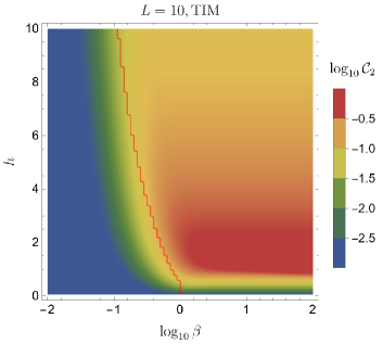
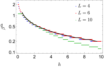
Figure 3: Top:Behaviour of $\mathcal{C}_{2}$ for model in Eq. (22) with $\kappa=0$ for different values if $\beta$ and $h$. The red line denotes the contour of $\mathcal{N}=10^{-4}$ to be used as an indicator to define lower bound of $\mathcal{C}_{2}$ to detect entanglement. Middle: Threshold $\mathcal{C}_{2}$ values which can be used to detect entanglement. Bottom:Threshold $\beta$ values above with $\mathcal{C}_{2}^{th}=0$ for different system sizes $L$. The black solid line denotes the moving average over $\delta h=0.1$

In the top panel of Fig. 3 we show the behaviour of $\mathcal{C}_{2}$ for a range of $\beta$ and $h$, while denoting the contour where $\mathcal{N}$ shows a non-zero value by red. Clearly for all values of $h$, $\mathcal{C}_{2}$ is an excellent witness of entanglement for $\beta>1$ i.e. at low temperature. For smaller $\beta$ we need to define a threshold value of $\mathcal{C}_{2}$, $\mathcal{C}_{2}^{th}$ to accurately detect entanglement. We show the numerically computed threshold values in the middle panel of Fig. 3. Two things are immediately apparent. The first is there is no significant finite size effect, in fact the threshold values reduce with system size which allows one to numerically compute the threshold for small system sizes and use them for experiments with a larger number of spins. Further accuracy can be achieved by a proper finite size analysis of the values which are beyond the scope of this work. The second prominent feature is the discrete ‘groupings’ of the values, which occurs due to discrete grid of $h$ and the finite tolerance available to detect $\mathcal{N}$. Finally in the bottom panel of Fig. 3, we plot the threshold value of $\beta$, $\beta^{th}$ for different $h$, which is defined as the smallest value of $\beta$ which allows for accurate detection of entanglement with $\mathcal{C}_{2}^{th}=0$. This also shows reduction with system size $L$.

Appendix E Example III — PXP model

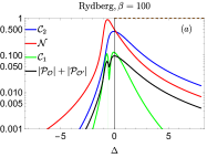
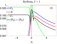
Figure 4: Plots showing comparison of behaviour of $\mathcal{C}_{2}$ and $\mathcal{C}_{1}$ defined in Eqs. (6) and (8), to Negativity $\mathcal{N}$ and the criterion in Eq. (5) for the model given in Eq. (49), (a) at $\beta=1/T=100$, (b) at $\beta=1$, The system size is $L=12$. The green grid line in panel (a) denotes the critical point.

As a final example, we consider the kinetically constrained Rydberg atom model which has recently gained a lot of attention due to presence of ‘quantum scars’. In particular we study entanglement detection for states in thermal equilibrium [Eq. (19)] obtained from the Hamiltonian,

$$H=\sum_{i=1}^{L}(\Omega\tilde{\sigma}_{i}^{x}+\Delta\sigma_{i}^{z})$$ (49)

and show that our method has the potential to be applied for entanglement witnessing. Mapping an empty Rydberg site to a down spin and a filled site to an up spin, we denote here $\tilde{\sigma}_{i}^{x}=P\sigma_{i}^{x}P$ operation where $P$ denotes projection to only those states in Hilbert space with no neighbouring up spins. It is known that this model has a ferromagnetic ground state with all spins pointing down, i.e., presence of zero excited Rydberg atoms when $\Delta\gg 0$ and $Z_{2}$ symmetry broken ground state for $\Delta\ll 0$. As shown in Fig. 4, at large $\beta=100$, different correlators behave similarly. In Fig. 4(a) we observe that while $\mathcal{N}$ shows a distinct peak at the known critical point of $\delta/\Omega=0.65$ and the maxima of $\mathcal{C}_{2}$ occurs at a slightly larger value. This is not unexpected as $\mathcal{C}_{2}$ is not an entanglement measure but a witness, hence we can only expect qualitative agreement. However, using Eq. (5) we cannot detect entanglement anywhere in the system as we never reach the threshold value of $1$. Expectedly, $\mathcal{C}_{1}$ shows completely different behaviour to $\mathcal{N}$ at low $\beta$ as seen Fig. 4(b) for a highly mixed state, where $\mathcal{C}_{2}$ qualitatively follows $\mathcal{N}$, but still there exists a region where $\mathcal{N}=0$ but $\mathcal{C}_{2}\neq 0$. Note that the agreement between $\mathcal{C}_{2}$ and $\mathcal{N}$ is more pronounced in this case than the Ising model, thus allowing for smaller cut-offs and providing better detection at larger temperatures. In Rydberg atoms, the change of basis can be simply executed experimentally via switching off the detuning field and the kinetic constraints by reducing the Rydberg blockade radius, and then taking a snapshot of the atomic density at different sites at $t=\frac{\pi}{4h}+2k\pi$,for $k\in\mathbb{Z}$, thus computing the correlation between the relevant subsystems.