Physics-based reduced-order modeling of flash-boiling sprays in the context of internal combustion engines

Abstract

Flash-boiling injection is one of the most effective ways to accomplish improved atomization compared to the high-pressure injection strategy. The tiny droplets formed via flash-boiling lead to fast fuel-air mixing and can subsequently improve combustion performance in engines. Most of the previous studies related to the topic focused on modeling flash-boiling sprays using three-dimensional (3D) computational fluid dynamics (CFD) techniques such as direct numerical simulations (DNS), large-eddy simulations (LES), and Reynolds-averaged Navier-Stokes (RANS) simulations. However, reduced order models can have significant advantages for applications such as the design of experiments, screening novel fuel candidates, and creating digital twins, for instance, because of the lower computational cost. In this study, the previously developed cross-sectionally averaged spray (CAS) model is thus extended for use in simulations of flash-boiling sprays. The present CAS model incorporates several physical submodels in flash-boiling sprays such as those for air entrainment, drag, superheated droplet evaporation, flash-boiling induced breakup, and aerodynamic breakup models. The CAS model is then applied to different fuels to investigate macroscopic spray characteristics such as liquid and vapor penetration lengths under flash-boiling conditions. It is found that the newly developed CAS model captures the trends in global flash-boiling spray characteristics reasonably well for different operating conditions and fuels. Moreover, the CAS model is shown to be faster by up to four orders of magnitude compared with simulations of 3D flash-boiling sprays. The model can be useful for many practical applications as a reduced-order flash-boiling model to perform low-cost computational representations of higher-order complex phenomena.

Abstract

Flash-boiling injection is one of the most effective ways to accomplish improved atomization compared to the high-pressure injection strategy. The tiny droplets formed via flash-boiling lead to fast fuel-air mixing and can subsequently improve combustion performance in engines. Most of the previous studies related to the topic focused on modeling flash-boiling sprays using three-dimensional (3D) computational fluid dynamics (CFD) techniques such as direct numerical simulations (DNS), large-eddy simulations (LES), and Reynolds-averaged Navier-Stokes (RANS) simulations. However, reduced order models can have significant advantages for applications such as the design of experiments, screening novel fuel candidates, and creating digital twins, for instance, because of the lower computational cost. In this study, the previously developed cross-sectionally averaged spray (CAS) model is thus extended for use in simulations of flash-boiling sprays. The present CAS model incorporates several physical submodels in flash-boiling sprays such as those for air entrainment, drag, superheated droplet evaporation, flash-boiling induced breakup, and aerodynamic breakup models. The CAS model is then applied to different fuels to investigate macroscopic spray characteristics such as liquid and vapor penetration lengths under flash-boiling conditions. It is found that the newly developed CAS model captures the trends in global flash-boiling spray characteristics reasonably well for different operating conditions and fuels. Moreover, the CAS model is shown to be faster by up to four orders of magnitude compared with simulations of 3D flash-boiling sprays. The model can be useful for many practical applications as a reduced-order flash-boiling model to perform low-cost computational representations of higher-order complex phenomena.

first-style=short

1 Introduction

Gasoline direct-injection spark-ignition (DISI) engines have been demonstrated to have the potential for higher thermal efficiencies than port-fuel injection (PFI) engines leading to lower fuel consumption and lower carbon dioxide ($\mathrm{CO_{2}}$) emissions [Leach et al., 2013]. DISI technology has several other advantages such as improved charge cooling potential, faster transient response, precise fuel metering, and lower cold start emissions [Reitz, 2013, Aleiferis and van Romunde, 2013, Yang et al., 2013, Zhao, 2010]. DISI engines use high-pressure injection systems for atomizing the liquid fuel into small droplets. Although an accurate control of fuel delivery, atomization, and good efficiency with reasonable emissions can be achieved via high-pressure injection systems, there are certain drawbacks associated with this injection mechanism. For example, due to high-pressure injection, the liquid fuel jet exits the injector nozzle normally with higher momentum, and thus increases the chances of spray impingement onto the cylinder liner and/or piston head [Xu et al., 2013]. The formation of a liquid film on the wall surface due to spray impingement will in turn affect the near-wall fuel-air mixing process [Zhao, 2021], as the fuel film is hard to evaporate and could lead to irregular combustion such as pool fire with subsequent production of soot and unburned hydrocarbons [Ratcliff et al., 2016, Xu et al., 2013]. Due to ever-increasing stringent emission regulations, the atomization characteristics of DISI engines also need to be improved further such that the resulting fine spray droplets from enhanced atomization lead to better fuel-air mixing with desired combustion characteristics [Xu et al., 2013]. Increasing injection pressure to extremely high values for achieving superior atomization characteristics has already been shown to be insufficient [Lefebvre, 1988]. However, the drawbacks mentioned above with the high-pressure injection strategy can be overcome by using the flash-boiling injection technique [Sun et al., 2021a, Yang et al., 2013].

Flash-boiling injection in DISI engines has become a promising alternative to generate a much finer spray compared to high-pressure injection [She, 2010, Schmitz et al., 2002, Fujimoto et al., 1997, Yamazaki et al., 1985]. Injecting liquid fuel into DISI engines operating at part-load, light-load, or idle conditions with early injection strategies for homogeneous-charge engine operation causes explosive vaporization of the fuel jet via bubble nucleation and growth [Badawy et al., 2022, Zeng et al., 2012]. This rapid phase-change phenomenon occurs due to the superheating of the liquid fuel upon entering the combustion chamber under the above-mentioned operating conditions. The potentially explosive nature of flash-boiling results in tiny droplets due to the abrupt disintegration of the liquid jet, which in turn enhances the mixture homogeneity between air and fuel by increasing the vaporization rate [Price et al., 2018], widening the spray plume due to the increased radial expansion via bubble growth, and reducing the droplet velocities, thus leading to shorter penetration [Badawy et al., 2022].

Flash-boiling consists of different sub-processes such as nucleation, bubble growth, and droplet burst [Senda et al., 1994]. The small length and time scales associated with these processes make it difficult to accurately quantify their influences on flash-boiling sprays [Dietzel, 2020, Price et al., 2018]. Many researchers have studied the flash-boiling phenomena at a microscopic single droplet level to have an in-depth understanding of the above-listed subprocesses (such as Saha et al. [2023, 2022, 2021], Wang et al. [2020], Xi et al. [2017], Li et al. [2017], among the most recent). Brown and York [1962] were the first to investigate the influence of flash-boiling at a macroscopic scale on the breakup and atomization process of superheated water and freon-11 jets. Sher and Elata [1977] quantified the flash-boiling spray formed by the binary mixture of toluene and freon 22 from pressure cans in terms of droplet size distributions for different pressures and temperatures. Adachi et al. [1997] reported a significant increase in fuel vapor concentration and subsequently more homogeneous fuel-air mixture formation from their experimental and theoretical investigations on the atomization process of superheated n-pentane sprays. Vanderwege and Hochgreb [1998] studied the effect of fuel volatility on sprays from high-pressure swirl injectors for fuel mixtures of doped and undoped iso-octane and indolene, and reported a 40$\%$ reduction in droplet diameter under flash-boiling conditions. Kale and Banerjee [2019] investigated the flash-boiling behavior of alcohol fuels using a direct-injection (DI) injector under engine-like hot injector body conditions. They also reported a significant reduction in droplet diameter (58.45$\%$ and 54.5$\%$ for butanol and iso-butanol, respectively) at elevated fuel temperatures due to the occurrence of flash-boiling. Senda et al. [2008] performed experiments with fuel mixtures of n-tridecane and liquefied $\mathrm{CO_{2}}$ to investigate the flash-boiling spray combustion characteristics. They found that the flash-boiling of the fuel mixture leads to a significant reduction in soot and $\mathrm{NO_{x}}$ emissions. The brake-specific fuel consumption was also observed to decrease due to the formation of an advanced flammable mixture resulting from flash-boiling. Aleiferis et al. [2010a] and Serras-Pereira et al. [2010] studied the combined effect of cavitation and flash-boiling on spray characteristics of different fuels using an optical DI injector nozzle. They revealed that an increase in the cavitation phenomenon inside the nozzle hole at higher fuel temperatures results in a large number of vapor bubbles, which then act as a strong source of nucleation sites and lead to an increase in the rate of superheated fuel vaporization. Several other experimental studies on flash-boiling injection are available in the literature (such as Sun et al. [2021b, 2020], Guo et al. [2018, 2017b], Mojtabi et al. [2014], Aleiferis et al. [2010b], to name a few), which confirm the potential of flash-boiling sprays in producing superior spray atomization along with improved combustion characteristics in DISI engines.

However, the characteristics of flash-boiling sprays deteriorate depending on the degree of superheating and the number and vicinity of the nozzle holes. With increasing superheating degrees, the radial expansion of the flash-boiling spray plumes increases, which may increase the possibility of jet-to-jet interactions and consequently the collapsing of the spray plumes. The collapsed flash-boiling sprays are associated with higher momentum flux and may lead to an increase in piston wall-wetting due to spray impingement [Duronio et al., 2021, Li et al., 2019, 2018b] and lubricant dilution, which are known to be one of the main sources of super-knock and engine damage [Wang et al., 2017a]. Studies on the collapsed flash-boiling spray characteristics and the detailed mechanism behind the spray collapse can be found in the literature (such as Zhou et al. [2018], Li et al. [2018a], Wang et al. [2017b, c], Guo et al. [2017a], to name a few).

Significant efforts were also made in developing numerical methods for modeling flash-boiling spray characteristics. Zuo et al. [2000] presented a superheated spray and vaporization model for studying the evolution and vaporization behavior of flashing sprays in GDI engines. Zeng and Lee [2001] developed an atomization model for flash-boiling sprays and concluded that the combined effect of aerodynamic forces and bubble expansion is responsible for breakup under flash-boiling conditions. Kawano et al. [2004] integrated the bubble nucleation, growth, and disruption sub-models into the KIVA3V code, and numerically investigated the flash-boiling characteristics of multicomponent fuels. Price et al. [2016] proposed a numerical framework for modeling flash-boiling sprays using a Lagrangian particle tracking (LPT) technique. The spray collapse and recirculations of droplets were well predicted by their model in comparison with the experimental measurements. Price et al. [2018] later applied this model to investigate the flash-boiling spray characteristics of high-volatility fuels (such as n-pentane, n-hexane, iso-hexane, and ethanol) as well as low-volatility fuels (such as iso-octane and n-butanol) over a wide range of injection systems. Guo et al. [2019] numerically investigated the flashing n-hexane sprays using the homogeneous relaxation model (HRM) in a diffuse Eulerian framework. They observed an under-expanded flashing jet due to the explosive evaporation within the intact liquid core, which was found to exist in the near nozzle regime. With increasing superheating degrees, the shock-wave structure, known as ‘Mach-disk’, was also identified at some distance from the nozzle exit. Duronio et al. [2021] developed a Lagrangian flash-boiling breakup model in OpenFOAM and studied the spray characteristics of the Engine Combustion Network (ECN) Spray G injector under flash boiling conditions for different injection pressures. Duronio et al. [2022] later simulated the internal nozzle flow in an Eulerian framework using the HRM model and coupled it with their previously developed Lagrangian external spray simulations to investigate the effect of in-nozzle phase change on global spray characteristics. Table 1 and Table 2 provide a comprehensive summary of the experimental and computational analysis contents of flash-boiling sprays, respectively, from several preceding studies mentioned earlier.

Although the three-dimensional (3D) computational fluid dynamics (CFD) simulations are necessary to get a detailed fundamental understanding of the underlying physics of the flash-boiling phenomena, the high computational cost associated with these simulations makes their application in the design of experiments, system simulations, creating digital twins, and screening of novel fuel candidates difficult. Model order reduction from 3D to 1D or 0D while preserving the essential multiphysics information is therefore useful as long as sufficient accuracy can be achieved. For example, in the fuel design process, each and every fuel candidate needs to undergo an extensive testing process before being used in real combustion systems. Assessing the spray characteristics and combustion performance is one of the crucial steps in this testing phase. However, conducting experiments on an engine test bench to investigate the spray and combustion characteristics for a large number of fuel candidates is extremely difficult [Deshmukh et al., 2022b]. The physics-based reduced-order models (ROM) can also be used as a digital twin of the internal combustion engine for closed-loop feedback control of the combustion performance [Deshmukh et al., 2022b]. Moreover, the simplicity of these ROMs allows for their interactive utilization with multi-dimensional spray simulations, as previously demonstrated by Wan [1997].

Sazhin et al. [2001] proposed simplified analytical expressions for obtaining the spray tip penetration during the initial stages and the later two-phase flow regimes. Desantes et al. [2006] derived a theoretical model to investigate the influence of the injection parameters on the macroscopic spray characteristics based on the assumption of the conservation of the momentum flux along the spray axis. Pastor et al. [2008] investigated the global spray characteristics of the transient inert diesel sprays using a 1D Eulerian spray model considering the mixing-controlled processes and locally-homogeneous flow field. Later, Desantes et al. [2009] extended it to reactive diesel spray cases. However, the droplet dynamics were neglected in these 1D Eulerian spray models. Wan [1997] was the first to derive a 1D cross-sectionally averaged spray model (CAS) from 3D multiphase governing equations for diesel sprays in the context of compression-ignition (CI) engines considering droplet dynamics. Recently, Deshmukh et al. [2022b] proposed some crucial improvements to the original CAS model by incorporating an additional vapor transport equation and state-of-the-art droplet breakup and evaporation models and found that the CAS model is able to predict the trend in inert subcooled spray characteristics reasonably well compared to the original work by Wan [1997] for different fuels under a wide range of operating conditions. They also extended the CAS model later to reactive turbulent spray cases [Deshmukh et al., 2022a]. Although considerable efforts have been made to the development of the ROMs for subcooled sprays, studies on the 1D physics-based ROM development for macroscopic characterization of the flash-boiling sprays are still scarce in the literature. Most computational studies on flash-boiling sprays are based on a 3D CFD approach. In this work, the CAS model developed by Deshmukh et al. [2022b] is further extended for the simulation of flash-boiling sprays. The extended CAS model is applied to different fuels under engine-like conditions, which are susceptible to flash-boiling. It incorporates several important physical sub-processes in flash-boiling sprays including air entrainment, drag, droplet internal as well as external vaporization, droplet heating, flash-boiling induced breakup, and aerodynamic breakup models. The proposed physics-based ROM for flash-boiling sprays is found to capture reasonably the trends in spray penetration lengths for different fuels under flash-boiling conditions.

The remaining manuscript is structured as follows. Section 2 introduces the new extended CAS model in detail. The numerical methods and the solution procedure are briefly discussed in Section 3. The detailed description of the experimental cases used for model validation is presented in Section 4. In Section 5, the macroscopic spray characteristics predicted by the previous CAS model as well as the newly developed CAS model are discussed. Finally, the findings of the present study are summarized in Section 6.

Year	Authors	Experiment details
1962	Brown and York [1962]	Exploration of the influence of flash-boiling at macroscopic scale on the atomization processes
1977	Sher and Elata [1977]	Quantification of droplet size distributions over a wide range of flash-boiling conditions
1997	Adachi et al. [1997]	Fuel vapor concentration characterization in n-pentane flash-boiling sprays
1998	Vanderwege and Hochgreb [1998]	Study of the effect of fuel volatility on flash-boiling sprays in high-pressure swirl injectors
2002	Schmitz et al. [2002]	Investigation of the impact of injector temperature on DI gasoline engine flash-boiling sprays
2008	Senda et al. [2008]	Characterization of flash-boiling spray combustion
2010	Aleiferis et al. [2010a]	Study of the influence of cavitation on flash-boiling behavior of hydrocarbon and alcohol fuels
2010	She [2010]	Impact of high-temperature flash-boiling on homogeneous-charge compression ignition diesel engine performance
2012	Zeng et al. [2012]	Multi-hole injector flash-boiling spray characteristics for alcohol fuels
2017	Li et al. [2017]	Quantitative investigation of the droplets morphology variation and breakup process in flash-boiling ethanol fuels
2019	Kale and Banerjee [2019]	Study of alcohol fuels flash-boiling behavior using DI injector
2020	Wang et al. [2020]	Investigation of bubble nucleation and micro-explosion phenomena in superheated jatropha oil droplets
2022	Badawy et al. [2022]	Effect of fuel temperature, ambient pressure, and fuel properties on multi-hole injector flash-boiling sprays

Table 1: Previous experimental studies on flash-boiling single droplets and sprays.

Year	Authors	Simulation details
1994	Senda et al. [1994]	Analytical modeling of atomization and evaporation processes in flash-boiling sprays
2000	Zuo et al. [2000]	Comprehensive modeling of superheated vaporization and breakup processes in GDI engines
2001	Zeng and Lee [2001]	Modeling of atomization process in flash-boiling sprays
2004	Kawano et al. [2004]	Modeling of atomization and vaporization processes in multi-component flash-boiling sprays
2017	Xi et al. [2017]	Lagrangian modeling of single droplet flash-boiling
2018	Price et al. [2018]	Lagrangian modeling of multi-hole flash-boiling spray over a broad range of injection systems and operating conditions
2017	Guo et al. [2019]	Eulerian modeling of flash-boiling characteristics of n-hexane fuel
2021	Duronio et al. [2021]	Lagrangian modeling of iso-octane flash-boiling behavior in ECN Spray G injector
2022	Duronio et al. [2022]	Investigation of the influence of in-nozzle phase change on flash-boiling spray using a combined Eulerian-Lagrangian framework
2020	Dietzel [2020]	Modeling of the influence of bubble interactions in flash-boiling cryogenic liquids using DNS
2022	Saha et al. [2022]	Modeling of single droplet flash-boiling behavior of e-fuels considering internal and external vaporization process
2023	Saha et al. [2023]	Reduced-order modeling of the influence of bubble interactions in highly volatile e-fuel microdroplets

Table 2: Previous simulation studies on flash-boiling single droplets and sprays.

2 Cross-sectionally averaged spray (CAS) model

The 3D multiphase governing equations for a complete spray [Hiroyasu and Arai, 1980] are reduced to 2D by assuming azimuthal symmetry and then radially integrated to obtain a one-dimensional system of equations. The reader is referred to Wan [1997] for more details about the model reduction. The governing equations (GEs) for the newly developed CAS model are given by

$$\mathrm{D_{g}}(\bar{\rho}\hat{Y}_{\mathrm{a}}b^{2}) =\dot{\omega}_{\mathrm{ent,\mathrm{a}}}b,$$ (1)

$$\mathrm{D_{g}}(\bar{\rho}\hat{Y}_{\mathrm{v}}b^{2}) =\left\langle\dot{\omega}_{\mathrm{vap,ext}}+\dot{\omega}_{\mathrm{vap,exp}}\right\rangle b^{2},$$ (2)

$$\mathrm{D_{g}}((\bar{\rho}\hat{Y}_{\mathrm{g}}\hat{u}_{\mathrm{g}}b^{2}) =-\left\langle\dot{\omega}_{\mathrm{drag}}\right\rangle b^{2}+\left\langle\dot{\omega}_{\mathrm{vap,ext}}+\dot{\omega}_{\mathrm{vap,exp}}\right\rangle\hat{u}_{\mathrm{l}}b^{2},$$ (3)

$$\mathrm{D_{g}}(\bar{\rho}\hat{Y}_{\mathrm{g}}\hat{T}_{\mathrm{g}}b^{2}) =-\left\langle\dot{\omega}_{\mathrm{heat}}\right\rangle\frac{C_{\mathrm{l}}}{C_{\mathrm{p,\mathrm{g}}}}b^{2}+\left\langle\left(\dot{\omega}_{\mathrm{vap,ext}}+\dot{\omega}_{\mathrm{vap,exp}}\right)\right\rangle\frac{C_{\mathrm{p,\mathrm{v}}}}{C_{\mathrm{p,\mathrm{g}}}}\hat{T}_{\mathrm{v}}b^{2}+\dot{\omega}_{\mathrm{ent,\mathrm{a}}}\frac{C_{\mathrm{p,\mathrm{a}}}}{C_{\mathrm{p,\mathrm{g}}}}\hat{T}_{\mathrm{a}}b,$$ (4)

$$\mathrm{D_{l}}((\bar{\rho}\hat{Y}_{\mathrm{l}}b^{2}) =-\left\langle\dot{\omega}_{\mathrm{vap,ext}}+\dot{\omega}_{\mathrm{vap,exp}}\right\rangle b^{2},$$ (5)

$$\mathrm{D_{l}}((\bar{\rho}\hat{Y}_{\mathrm{l}}\hat{u}_{\mathrm{l}}b^{2}) =\left\langle\dot{\omega}_{\mathrm{drag}}\right\rangle b^{2}-\left\langle\dot{\omega}_{\mathrm{vap,ext}}+\dot{\omega}_{\mathrm{vap,exp}}\right\rangle\hat{u}_{\mathrm{l}}b^{2},$$ (6)

$$\mathrm{D_{l}}(\bar{\rho}\hat{Y}_{\mathrm{l}}\langle\hat{d_{\mathrm{d}}}\rangle b^{2}) =-\left\langle\frac{\dot{\omega}_{\mathrm{bre}}}{2\hat{d_{\mathrm{d}}}}\right\rangle b^{2}-\frac{4}{3}\left\langle\dot{\omega}_{\mathrm{vap,ext}}\hat{d_{\mathrm{d}}}\right\rangle b^{2}-\frac{2}{3}\left\langle\dot{\omega}_{\mathrm{vap,exp}}\hat{d_{\mathrm{d}}}\right\rangle b^{2},$$ (7)

$$\mathrm{D_{l}}(\bar{\rho}\hat{Y}_{\mathrm{l}}\hat{T}_{\mathrm{d}}b^{2}) =\left\langle\dot{\omega}_{\mathrm{heat}}\right\rangle b^{2}-\left\langle\left(\dot{\omega}_{\mathrm{vap,ext}}+\dot{\omega}_{\mathrm{vap,exp}}\right)\right\rangle\hat{T}_{\mathrm{d}}b^{2},$$ (8)

where $\rho$ denotes the density, $b(z,t)$ the spray width, $z$ the axial coordinate, $t$ the temporal coordinate, $Y$ the mass fraction, $u$ the velocity, $d$ the droplet diameter, $C$ the specific heat capacity, $C_{\text{p}}$ the specific heat capacity at constant pressure, and $T$ the temperature. The subscripts ‘d’, ‘l’, ‘g’, ‘a’, and ‘v’ refer to the droplet variables, liquid phase, gas phase, ambient gas, and vapor, respectively. The radially integrated differential operator, $\mathrm{D}_{\text{i}}(\bar{\rho}\hat{\phi}b^{2})$, is defined as

$$\mathrm{D}_{\text{i}}(\bar{\rho}\hat{\phi}b^{2})=\frac{\partial}{\partial t}(\bar{\rho}\hat{\phi}b^{2})+\frac{\partial}{\partial z}(\bar{\rho}\hat{\phi}\hat{u}_{\mathrm{i}}b^{2})\hskip 14.22636pt\text{ with}\hskip 14.22636pti=\mathrm{g,\,l}\text{,}$$ (9)

where $\phi$ represents the quantity of interest. The density-weighted cross-sectional average of $\phi$ is defined as

$$\bar{\rho}\hat{\phi}b^{2}=2\int_{0}^{\infty}\rho\phi r\mathrm{~{}d}r,$$ (10)

where $r$ is the radial coordinate. The cross-sectional averaging with $\phi=1$ and density-weighted cross-sectional averaging are denoted by the ‘overline’ ($\bar{\cdot}$) and ‘hat’ ($\hat{\cdot}$) operators, respectively. The operator, $\langle\cdot\rangle$, in the GEs represents the expectation value of any term, $\zeta(\hat{d_{\mathrm{d}}})$, which is a function of droplet diameter and is defined as

$$\langle\zeta\rangle=\int\zeta(\hat{d}^{\prime})\mathcal{P}(\hat{d}^{\prime})\mathrm{d}\hat{d}^{\prime},$$ (11)

where $\mathcal{P}(\hat{d}^{\prime})$ denotes the droplet size distribution. However, due to the difficulties associated with the use of polydisperse droplet size distribution [Deshmukh et al., 2022b], the droplets are assumed to be monodisperse in this study. A schematic of the CAS model is shown in Fig. 1. The source terms on the right-hand side of the GEs describe different sub-models for the physical processes, such as air-entrainment ($\dot{\omega}_{\mathrm{ent,\mathrm{a}}}$), drag ($\dot{\omega}_{\mathrm{drag}}$), heat transfer ($\dot{\omega}_{\mathrm{heat}}$), droplet breakup ($\dot{\omega}_{\mathrm{bre}}$), vaporization ($\dot{\omega}_{\mathrm{vap,ext}}$), and droplet expansion ($\dot{\omega}_{\mathrm{vap,exp}}$) in flash-boiling sprays. The details of the sub-models are discussed in the next subsections.

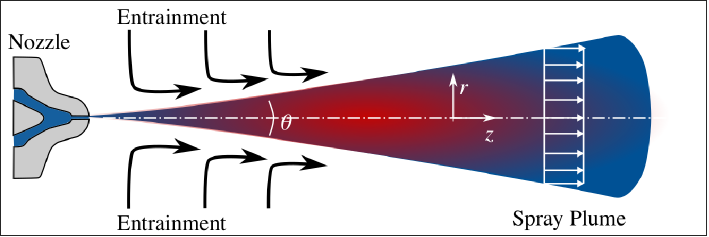
Figure 1: Schematic of the CAS model.

2.1 Air entrainment model

Air entrainment into the spray plume describes the air mass flow across the spray boundary. The spray morphology is significantly influenced by the entrained air [Ghandilou and Taghavifar, 2022]. The higher the entrainment rate, the better will be the mixing between the injected fuel and ambient air, and subsequently, the combustion performance will be improved. The air entrainment source term is modeled as [Deshmukh et al., 2022b]

$$\dot{\omega}_{\mathrm{ent},\mathrm{a}}=\rho_{\mathrm{a}}\beta\hat{u}_{\mathrm{g}},$$ (12)

where $\beta$ is the spreading coefficient defined as $\beta=\tan(\theta/2)$ and $\theta$ (in degree) the spray cone angle.

2.1.1 Spray cone angle model

The spray cone angle, which was previously modeled using the Hiroyasu and Arai [1980] correlation, is updated in this work for superheated conditions as [Price et al., 2018]

$$\theta=\log\left(\frac{R_{p}^{2}\Theta^{3}}{m_{\mathrm{a}}^{2}}\right),$$ (13)

where $R_{\mathrm{p}}$ denotes the ratio of saturated vapor pressure ($P_{\mathrm{v}}$) corresponding to the injection temperature ($T_{\mathrm{inj}}$) and ambient gas pressure ($P_{\mathrm{g}}$), and $m_{\mathrm{a}}$ the atomic mass of the injected fuel. $\Theta$ is the nondimensional surface tension defined as

$$\Theta=\frac{a\sigma}{k_{\mathrm{b}}T_{\mathrm{inj}}}\hskip 14.22636pt\text{ with}\hskip 14.22636pta=\left({36\pi}{v_{l}^{2}}\right)^{1/3}\text{,}$$ (14)

where $k_{\mathrm{b}}$ is the Boltzmann constant, $a$ the molecular surface area, $v_{l}$ the liquid molecular volume, and $\sigma$ the surface tension.

2.2 Drag model

The steady-state drag force on a droplet can be expressed as [Crowe et al., 2012]

$$F_{\mathrm{ss,drag}}=\frac{1}{2}\rho_{\mathrm{g}}C_{\mathrm{drag}}{A_{\mathrm{d}}}\left({u}_{\mathrm{g}}-{u}_{\mathrm{l}}\right)\left|{u}_{\mathrm{g}}-{u}_{\mathrm{l}}\right|,$$ (15)

where ${A_{\mathrm{d}}}$ is the droplet surface area and $C_{\mathrm{drag}}$ the droplet drag coefficient computed as [Wallis, 1969]

$$C_{\mathrm{drag}}=\left\{\begin{array}[]{ll}\frac{24}{\mathsf{Re}_{\mathrm{{d}}}}(1+\frac{1}{6}\mathsf{Re}_{\mathrm{{d}}}^{2/3})&\quad\text{for $\mathsf{Re}_{\mathrm{{d}}}\leq 1000$ }\\ 0.424&\quad\text{for $\mathsf{Re}_{\mathrm{{d}}}>1000$}.\end{array}\right.$$ (16)

$\mathsf{Re}_{\mathrm{{d}}}$ denotes the droplet Reynolds number and is given by

$$\mathsf{Re}_{\mathrm{{d}}}=\rho_{\mathrm{g}}\left|{u}_{\mathrm{g}}-{u}_{\mathrm{l}}\right|\hat{d_{\mathrm{d}}}/\mu_{\mathrm{g}},$$ (17)

where $\mu_{\mathrm{g}}$ is the gas-phase molecular viscosity. The source term due to the steady-state drag force on a droplet of diameter $\hat{d_{\mathrm{d}}}$ is thus computed as

$$\dot{\omega}_{\mathrm{drag}}=\frac{3C_{\mathrm{drag}}\rho_{\mathrm{g}}\bar{\rho}\hat{Y}_{\mathrm{l}}(\hat{u}_{\mathrm{g}}-\hat{u}_{\mathrm{l}})|\hat{u}_{\mathrm{g}}-\hat{u}_{\mathrm{l}}|}{4\rho_{\mathrm{l}}\hat{d_{\mathrm{d}}}}.$$ (18)

2.3 Superheated droplet breakup model

Deshmukh et al. [2022b] modeled the droplet breakup only via the aerodynamic breakup mechanism as the sub-cooled liquid droplet atomization is known to be mainly controlled by the aerodynamic forces acting on the droplet surface. However, for the flash-boiling droplet, the superheating degree plays an important role in determining the atomization characteristics. The spontaneous growth of the vapor bubbles and the aerodynamic forces compete with each other during the flash-boiling spray atomization process. Micro-explosions due to the bubble growth dominate in the regime of high superheating degrees, whereas aerodynamic forces dominate in low superheating degree regimes [Zeng and Lee, 2001]. Thus, in this work, the CAS model has been integrated with a hybrid breakup model which includes both the thermal and the aerodynamic breakup mechanisms.

A liquid droplet generates multiple child droplets at the end of the breakup. However, a continuous thermal and aerodynamic breakup approach is considered in the CAS model for simplicity, which results in a continuous reduction of the droplet diameter rather than generating multiple child droplets [Deshmukh et al., 2022b]. The source term due to the droplet breakup is expressed as $\dot{\omega}_{\mathrm{bre}}=K_{\mathrm{bre}}\bar{\rho}$, where $K_{\mathrm{bre}}$ is the breakup coefficient modeled either via $K_{\mathrm{bre,thm}}$ or via $K_{\mathrm{bre,aero}}$ depending on the breakup length and time scales. $K_{\mathrm{bre,thm}}$ and $K_{\mathrm{bre,aero}}$ describe the breakup coefficients resulting from the micro-explosion (herein referred to as ‘thermal breakup’) and aerodynamic force-induced breakup (herein referred to as ‘aerodynamic breakup’) mechanism, respectively. Details on the calculation of the breakup coefficients are discussed in the following subsections.

2.3.1 Thermal breakup

The breakup coefficient of the thermal breakup is modeled as

$$K_{\mathrm{bre,thm}}=\frac{2\hat{d_{\mathrm{d}}}(\hat{d_{\mathrm{d}}}-d_{\mathrm{st,thm}})}{\tau_{\mathrm{b,thm}}}\hskip 14.22636pt\text{with}\hskip 14.22636pt\tau_{\mathrm{b,thm}}=A_{0}\frac{\hat{d_{\mathrm{d}}}}{\eta_{\mathrm{thm}}\Omega_{\mathrm{thm}}}\hskip 11.38092pt\text{and}\hskip 11.38092ptd_{\mathrm{st,thm}}=A_{1}\eta_{\text{thm}},$$ (19)

where $d_{\mathrm{st,thm}}$ and $\tau_{\mathrm{b,thm}}$ denote the stable droplet diameter and breakup time associated with the thermal breakup mechanism, respectively. The amplitude of the disturbance due to the bubble growth ($\eta_{\text{thm}}$) and the disturbance growth rate ($\Omega_{\mathrm{thm}}$) are defined as

$$\eta_{\mathrm{thm}}=\left(\frac{6\epsilon_{\mathrm{crit}}V_{\mathrm{l}}}{\pi N_{\mathrm{bub}}\left(1-\epsilon_{\mathrm{crit}}\right)}\right)^{1/3}\hskip 14.22636pt\text{and}\hskip 14.22636pt\Omega_{\mathrm{thm}}=\frac{2\dot{R}_{\mathrm{b}}}{\mathsf{D_{o}}}\hskip 14.22636pt\text{with}\hskip 14.22636pt\dot{R}_{\mathrm{b}}=\sqrt{\frac{2}{3}\frac{P_{\mathrm{v}}\left(\hat{T}_{\mathrm{d}}\right)-P_{\mathrm{g}}}{\rho_{\mathrm{l}}}},$$ (20)

where $\epsilon_{\mathrm{crit}}$ denotes the critical void fraction given by $\epsilon_{\mathrm{crit}}=V_{\mathrm{b}}/\left(V_{\mathrm{b}}+V_{\mathrm{l}}\right)$. $V_{\mathrm{b}}$ and $V_{\mathrm{l}}$ are the total volume of the vapor bubbles and liquid in the superheated droplet, respectively. In the CAS model, a value of 0.55 is considered for $\epsilon_{\mathrm{crit}}$ [Kawano et al., 2004]. $N_{\mathrm{bub}}$ represents the total number of vapor bubbles in the superheated droplet and is calculated using the empirical bubble number density proposed by Senda et al. [1994] as

$$n=5.757\times 10^{12}\cdot\exp\left(\frac{-5.279\mathrm{~{}K}}{\Delta T}\right)\hskip 14.22636pt\text{with}\hskip 14.22636pt\Delta T=T_{\mathrm{inj}}-{T_{\mathrm{b}}}(P_{\mathrm{g}}),$$ (21)

where $\Delta T$ is the superheating degree of the liquid droplet.

2.3.2 Aerodynamic breakup

A combined Kelvin–Helmholtz (KH) - Rayleigh–Taylor (RT) breakup model is incorporated in the CAS model for the aerodynamic breakup. The aerodynamic breakup coefficient is expressed as

$$K_{\mathrm{bre,aero}}=\frac{2\hat{d_{\mathrm{d}}}(\hat{d_{\mathrm{d}}}-d_{\mathrm{st,aero}})}{\tau_{\mathrm{b,aero}}}.$$ (22)

The stable droplet diameter ($d_{\mathrm{st,aero}}$) and breakup time ($\tau_{\mathrm{b,aero}}$) associated with the aerodynamic breakup are computed either via the KH model as

$$d_{\mathrm{st,KH}}=2B_{0}\Lambda_{\mathrm{KH}},\hskip 14.22636pt\tau_{\mathrm{b,KH}}=3.788B_{1}\frac{\hat{d_{\mathrm{d}}}}{2\Lambda_{\mathrm{KH}}\Omega_{\mathrm{KH}}}$$ (23)

or via the RT model as

$$d_{\mathrm{st,RT}}=C_{3}\Lambda_{\mathrm{RT}},\hskip 14.22636pt\tau_{\mathrm{b,RT}}=\Omega_{\mathrm{RT}}^{-1},$$ (24)

where $\Lambda$ is the wavelength of the fastest-growing wave and $B_{0}$ the model constant equal to 0.61. The detailed calculation of $\Lambda$ and $\Omega$ corresponding to the KH-RT breakup model can be found in Patterson and Reitz [1998].

The breakup is modeled via the thermal breakup mechanism if $\hat{d_{\mathrm{d}}}>d_{\mathrm{st,thm}}$ and $\tau_{\mathrm{b,thm}}<\tau_{\mathrm{b,aero}}$, otherwise, the breakup takes place via the aerodynamic breakup mechanism. The RT model is used for aerodynamic breakup if $\hat{d_{\mathrm{d}}}>d_{\mathrm{st,RT}}$ and $\tau_{\mathrm{b,RT}}<\tau_{\mathrm{b,KH}}$, else the KH model is considered. The breakup model constants, $A_{0}$, $A_{1}$, $B_{1}$, and $C_{3}$, depend on the injector nozzle geometry and therefore need to be tuned for a given injector to match the experimental liquid length [Deshmukh et al., 2022b]. It is to be noted that for a given injector, once the tuning is performed, the breakup model can be used for any fuel under any operating conditions without further tuning the model constants.

2.4 Superheated droplet vaporization model

Deshmukh et al. [2022b] previously modeled evaporation using the Miller and Bellan [1999] model, which is not valid for superheated droplets. The phase transition in superheated liquid droplets occurs in two distinct ways: (1) by spontaneous nucleation and subsequent growth of the vapor bubbles in the droplet, herein referred to as ‘internal vaporization’, and (2) by vaporization from the droplet’s external surface due to the internal as well as external temperature gradient, herein referred to as ‘external vaporization’ [Yang, 2017, Saha et al., 2022]. The evaporation model in the CAS formulation is thus updated with the above-mentioned vaporization phenomena.

2.4.1 Internal vaporization

The internal vaporization via the formation of vapor bubbles causes the droplet to expand in the radially outward direction in the superheated regime. A schematic of the internal vaporization process is shown in Fig. 2. The source term of droplet expansion is modeled as

$$\dot{\omega}_{\mathrm{vap,exp}}=\frac{3K_{\mathrm{vap,exp}}\bar{\rho}\hat{Y}_{\mathrm{l}}}{2\hat{d}^{2}_{\mathrm{d}}},$$ (25)

where $K_{\mathrm{vap,exp}}$ is expressed as [Saha et al., 2023]

$$K_{\mathrm{vap,exp}}=\frac{4\hat{d_{\mathrm{d}}}\rho_{v}\dot{R}_{\mathrm{b}}}{\rho_{l}}N_{\text{bub}}.$$ (26)

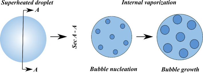
Figure 2: Schematic of the internal vaporization process [Saha et al., 2023].

2.4.2 External vaporization

The superheated liquid droplet undergoes a phase change from its external surface due to the heat transfer from the inner core of the droplet. The external phase transition may also take place due to the temperature gradient between the droplet outer interface and the ambient gas. The source term for the vaporization due to the heat flux from the droplet’s inner core is modeled as $\dot{\omega}_{\mathrm{vap,ht1}}={3K_{\mathrm{vap,ht1}}\bar{\rho}\hat{Y}_{\mathrm{l}}}/({2\hat{d}^{2}_{\mathrm{d}}})$. The vaporization coefficient, $K_{\mathrm{vap,ht1}}$, is given by [Adachi et al., 1997]

$$K_{\mathrm{vap,ht1}}=\frac{4\hat{d_{\mathrm{d}}}h_{\mathrm{1}}(\hat{T}_{\mathrm{d}}-{T_{\mathrm{b}}})}{\rho_{l}L\left({T_{\mathrm{b}}}\right)},$$ (27)

where ${T_{\mathrm{b}}}$ denotes the droplet boiling temperature and $L$ is the latent heat of vaporization at ${T_{\mathrm{b}}}$. The internal heat transfer coefficient, $h_{\mathrm{1}}$ (in kW/m²K), is approximated as [Adachi et al., 1997]

$$h_{\mathrm{1}}=\left\{\begin{array}[]{ll}0.76(\hat{T}_{\mathrm{d}}-T_{\mathrm{b}})^{0.26}&(0<\hat{T}_{\mathrm{d}}-T_{\mathrm{b}}<5)\\ 0.027(\hat{T}_{\mathrm{d}}-T_{\mathrm{b}})^{2.33}&(5<\hat{T}_{\mathrm{d}}-T_{\mathrm{b}}<25)\\ 13.8(\hat{T}_{\mathrm{d}}-T_{\mathrm{b}})^{0.39}&(\hat{T}_{\mathrm{d}}-T_{\mathrm{b}}>25).\end{array}\right.$$ (28)

The vaporization source term due to the temperature gradient between the droplet’s external surface and the surrounding gas is modeled as $\dot{\omega}_{\mathrm{vap,ht2}}={3K_{\mathrm{vap,ht2}}\bar{\rho}\hat{Y}_{\mathrm{l}}}/({2\hat{d}^{2}_{\mathrm{d}}})$, where the vaporization coefficient, $K_{\mathrm{vap,ht2}}$, is given by [Adachi et al., 1997]

$$K_{\mathrm{vap,ht2}}=\frac{4\hat{d_{\mathrm{d}}}f_{3}h_{\mathrm{2}}|\hat{T}_{\mathrm{g}}-\hat{T}_{\mathrm{s}}|}{\rho_{l}L(\hat{T}_{\mathrm{s}})},$$ (29)

where $h_{\mathrm{2}}$ represents the external heat transfer coefficient and $\hat{T}_{\mathrm{s}}$ the droplet surface temperature, which is assumed to be equal to ${T_{\mathrm{b}}}$ in the superheated regime [Saha et al., 2022]. The additional Stefan flow caused by the mass flux due to the heat transfer from the droplet’s inner core counteracts the external temperature gradient-based vaporization process and may significantly reduce the heat flux to/from the droplet’s outer surface [Zuo et al., 2000]. The factor $f_{3}$ is an evaporative heat transfer correction factor, which is introduced here to take into account the above-mentioned phenomena, and is defined as

$$f_{3}=\frac{1}{1-\text{PR}}\hskip 14.22636pt\text{with}\hskip 14.22636pt\text{PR}=\frac{P_{\mathrm{g}}}{P_{\mathrm{v}}(\hat{T}_{\mathrm{d}})}.$$ (30)

Combining the contributions from the different external vaporization sources, such as $\dot{\omega}_{\mathrm{vap,ht1}}$ and $\dot{\omega}_{\mathrm{vap,ht2}}$, yields the source term due to the total external vaporization in the superheated regime as

$$\dot{\omega}_{\mathrm{vap,ext}}=\frac{3K_{\mathrm{vap,ext}}\bar{\rho}\hat{Y}_{\mathrm{l}}}{2\hat{d}^{2}_{\mathrm{d}}}\hskip 14.22636pt\text{with}\hskip 11.38092ptK_{\mathrm{vap,ext}}=K_{\mathrm{vap,ht1}}+K_{\mathrm{vap,ht2}}.$$ (31)

When the superheated liquid droplet cools down to a temperature below ${T_{\mathrm{b}}}$, the standard non-equilibrium evaporation model proposed by Miller and Bellan [1999] is used to model the vaporization process. The vaporization coefficient in this sub-cooled regime is given by [Deshmukh et al., 2022b]

$$K_{\mathrm{vap,ext}}=4\frac{\rho_{\mathrm{g}}\mathit{\Gamma}_{\mathrm{v,g}}}{\rho_{\mathrm{l}}}\;\mathrm{ln}(1+\mathsf{B_{M,\mathrm{{d}}}})\mathsf{Sh_{\mathrm{{d}}}},$$ (32)

where $\mathit{\Gamma}_{\mathrm{v,g}}$ denotes the diffusion coefficient of fuel vapor in the ambient gas mixture and $\mathsf{B_{M,\mathrm{{d}}}}$ is the Spalding mass transfer number. The Sherwood number, $\mathsf{Sh_{\mathrm{{d}}}}$, is computed using the Ranz and Marshall [1952] correlation as

$$\mathsf{Sh_{\mathrm{{d}}}}=2+0.552~{}\mathsf{Re}_{\mathrm{{d}}}^{1/2}~{}\mathsf{Sc_{\mathrm{{g}}}}^{1/3},\\$$ (33)

where the gas-phase Schmidt number, $\mathsf{Sc_{\mathrm{{g}}}}$, is defined as

$$\mathsf{Sc_{\mathrm{{g}}}}=\frac{\mu_{\mathrm{g}}\left(T_{\mathrm{ref}}\right)}{\rho_{\mathrm{g}}\left(T_{\mathrm{ref}}\right)\mathit{\Gamma}_{\mathrm{v,g}}\left(T_{\mathrm{ref}}\right)}.$$ (34)

For additional details on the subcooled vaporization modeling, the reader is referred to Deshmukh et al. [2022b]. In the CAS model, the liquid properties such as density ($\rho_{\mathrm{l}}$), viscosity ($\mu_{\mathrm{l}}$), and surface tension ($\sigma$) are assumed to be constant throughout the liquid phase and computed at the injection temperature ($T_{\mathrm{inj}}$). The Wilke [1950] formula is used to evaluate the gas-phase mixture properties such as viscosity ($\mu_{\mathrm{g}}$) and thermal conductivity ($\lambda_{\mathrm{g}}$), whereas the mixture-specific heat capacity at constant pressure ($C_{\mathrm{p,\mathrm{g}}}$) is evaluated using the linear mixing rule [Deshmukh et al., 2022b]. All the gas-phase mixture properties and the correlations in the CAS model are computed at reference temperature ($T_{\mathrm{ref}}$) obtained by the one-third rule [Hubbard et al., 1975]. The derivation of the vaporization coefficients is provided in A.

2.5 Gas-phase energy transport

Deshmukh et al. [2022b] calculated the gas phase temperature, $\hat{T}_{\mathrm{g}}$, by assuming a homogeneous mixture of fuel vapor and ambient gas. In the present work, a more accurate formulation has been incorporated for obtaining $\hat{T}_{\mathrm{g}}$ considering the following physical phenomena: (1) the energy dissipation/deposition due to the heat transfer between the droplets and the gas-phase denoted by ${\dot{\omega}_{\mathrm{heat}}}(C_{\mathrm{l}}/C_{\mathrm{p,\mathrm{g}}})b^{2}$, (2) the energy transport by the vaporized fuel into the gas phase expressed as ${\left(\dot{\omega}_{\mathrm{vap,ext}}+\dot{\omega}_{\mathrm{vap,exp}}\right)}(C_{\mathrm{p,\mathrm{v}}}/C_{\mathrm{p,\mathrm{g}}})\hat{T}_{\mathrm{v}}b^{2}$, and (3) the energy transport by the fresh ambient air into the spray plume due to the air-entrainment phenomenon given by $\dot{\omega}_{\mathrm{ent,\mathrm{a}}}(C_{\mathrm{p,\mathrm{a}}}/C_{\mathrm{p,\mathrm{g}}})\hat{T}_{\mathrm{a}}b$. The fuel vapor temperature, $\hat{T}_{\mathrm{v}}$, in Eq. (4) is calculated based on the energy balance between the liquid and the fuel vapor as

$$\hat{T}_{\mathrm{v}}=\frac{C_{\mathrm{l}}\hat{T}_{\mathrm{d}}-L(\hat{T}_{\mathrm{s}})}{C_{\mathrm{p,\mathrm{v}}}}.$$ (35)

2.6 Heat transfer model

The droplet bulk temperature in the CAS model was calculated using the infinite-conductivity model proposed by Miller and Bellan [1999] only considering subcooled heat transfer. In this work, the energy balance equation has been updated for the superheated droplet as

$$\frac{\mathrm{d}\hat{T}_{\mathrm{d}}}{\mathrm{d}t}=\underbrace{\frac{6f_{\text{2,sup}}\mathsf{Nu_{\mathrm{{d}}}}\lambda_{\mathrm{g}}(T_{\mathrm{ref}})(\hat{T}_{\mathrm{g}}-\hat{T}_{\mathrm{s}})}{\rho_{\mathrm{l}}\hat{d}^{2}_{\mathrm{d}}C_{\mathrm{l}}(\hat{T}_{\mathrm{d}})}}_{\text{conductive heat flow}}-\underbrace{\overbrace{\frac{3K_{\mathrm{vap,ext}}L(\hat{T}_{\mathrm{s}})}{2\hat{d_{\mathrm{d}}}^{2}C_{\mathrm{l}}(\hat{T}_{\mathrm{d}})}}^{\text{external vaporization}}-\overbrace{\frac{3K_{\mathrm{vap,exp}}L(\hat{T}_{\mathrm{d}})}{2\hat{d_{\mathrm{d}}}^{2}C_{\mathrm{l}}(\hat{T}_{\mathrm{d}})}}^{\text{internal vaporization}}}_{\text{evaporative cooling}}=K_{\mathrm{heat}}.$$ (36)

The derivation of the heat transfer coefficient, $K_{\mathrm{heat}}$, is given in B. In Eq. (36), the first term on the right-hand side describes the conductive heat flow per unit time between the droplet surface and the external ambient. The second and third terms represent the evaporative cooling of the droplet due to external and internal vaporization, respectively. $f_{2}$ is the analytical evaporative heat transfer correction factor defined as

$$f_{\text{2,sup}}=\frac{\xi_{\text{sup}}}{e^{\xi_{\text{sup}}}-1}.$$ (37)

$\mathsf{Nu_{\mathrm{{d}}}}$ denotes the Nusselt number and is computed using Ranz and Marshall [1952] correlations as

$$\mathsf{Nu_{\mathrm{{d}}}}=2+0.552~{}\mathsf{Re}_{\mathrm{{d}}}^{1/2}~{}\mathsf{Pr_{\mathrm{{g}}}}^{1/3},$$ (38)

and $\xi_{\text{sup}}$ is the non-dimensional evaporation parameter under the superheated regime given by

$$\xi_{\text{sup}}=\left(\frac{\mathsf{Pr_{\mathrm{{g}}}}\hat{d_{\mathrm{d}}}}{2\mu_{\mathrm{g}}}\right)\left[\frac{h_{1}(\hat{T}_{\mathrm{d}}-\hat{T}_{\mathrm{s}})}{L(\hat{T}_{\mathrm{s}})}+\frac{f_{3}h_{2}|\hat{T}_{\mathrm{g}}-\hat{T}_{\mathrm{s}}|}{L(\hat{T}_{\mathrm{s}})}\right],$$ (39)

where $\mathsf{Pr_{\mathrm{{g}}}}$ is the gas-phase Prandtl number defined as

$$\mathsf{Pr_{\mathrm{{g}}}}=\frac{\mu_{\mathrm{g}}(T_{\mathrm{ref}})C_{\mathrm{p,\mathrm{g}}}(T_{\mathrm{ref}})}{\lambda_{\mathrm{g}}(T_{\mathrm{ref}})}.$$ (40)

For subcooled droplets, the conductive heat flow and the external vaporization are solely responsible for the change in droplet bulk temperature, and thus $K_{\mathrm{heat}}$ can be expressed as

$$K_{\mathrm{heat}}=\underbrace{\frac{6f_{\text{2,sub}}\mathsf{Nu_{\mathrm{{d}}}}\lambda_{\mathrm{g}}(T_{\mathrm{ref}})(\hat{T}_{\mathrm{g}}-\hat{T}_{\mathrm{s}})}{\rho_{\mathrm{l}}\hat{d}^{2}_{\mathrm{d}}C_{\mathrm{l}}(\hat{T}_{\mathrm{d}})}}_{\text{conductive heat flow}}-\underbrace{\overbrace{\frac{3K_{\mathrm{vap,ext}}L(\hat{T}_{\mathrm{s}})}{2\hat{d_{\mathrm{d}}}^{2}C_{\mathrm{l}}(\hat{T}_{\mathrm{d}})}}^{\text{external vaporization}}}_{\text{evaporative cooling}}\hskip 14.22636pt\text{with}\hskip 11.38092ptf_{\text{2,sub}}=\frac{\xi_{\text{sub}}}{e^{\xi_{\text{sub}}}-1}.$$ (41)

In the subcooled regime, $\hat{T}_{\mathrm{s}}$ is considered to be equal to the droplet bulk temperature $\hat{T}_{\mathrm{d}}$. The non-dimensional evaporation parameter in the subcooled regime, $\xi_{\text{sub}}$, is computed as [Deshmukh et al., 2022b]

$$\xi_{\text{sub}}=\frac{1}{2}\frac{\mathsf{Pr_{\mathrm{{g}}}}}{\mathsf{Sc_{\mathrm{{g}}}}}\;\mathrm{ln}(1+\mathsf{B_{M,\mathrm{{d}}}})\mathsf{Sh_{\mathrm{{d}}}}.$$ (42)

The source term due to heat transfer is thus modeled as

$$\dot{\omega}_{\mathrm{heat}}=K_{\mathrm{heat}}\bar{\rho}\hat{Y}_{\mathrm{l}}.$$ (43)

2.7 Nozzle exit conditions

A blob injection model [Reitz, 1987, Reitz and Diwakar, 1987] was incorporated by Deshmukh et al. [2022b] which injects the droplet with a diameter equivalent to the size of the effective nozzle hole diameter into the gas phase. However, during flash-boiling injection, near-nozzle droplet shattering due to rapid disintegration of the superheated liquid jet results in a significant reduction in droplet diameter at the nozzle exit (as low as $\sim$ 10 $\%$ of the nozzle hole diameter) [Price et al., 2020, 2016]. In-nozzle phase change due to cavitation may further enhance the near nozzle atomization characteristics of the superheated liquid jet [Gemci et al., 2004]. The use of an initial droplet of size comparable to the nozzle exit diameter at flash-boiling conditions would result in an unrealistic flash-boiling spray with no plume merging or spray collapse. The size of the initial droplet diameter is thus crucial in determining the global characteristics of a flash-boiling spray [Price et al., 2016, 2015]. In this work, the CAS model has been integrated with a correlation proposed by Gemci et al. [2004] to compute the initial droplet diameter ($\mathsf{D_{o}}$) as

$$\mathsf{D_{o}}=118.40-28.29\left(\Delta T^{*}-\text{CN}\right)\hskip 9.95863pt\text{with}\hskip 9.95863pt\Delta T^{*}=\frac{T_{\mathrm{inj}}-{T_{\mathrm{b}}}\left(P_{\mathrm{g}}\right)}{{T_{\mathrm{b}}}\left(P_{\mathrm{inj}}\right)-{T_{\mathrm{b}}}\left(P_{\mathrm{g}}\right)}\hskip 9.95863pt\text{and}\hskip 9.95863pt\text{CN}=\frac{P_{\mathrm{inj}}-P_{\mathrm{v}}\left(T_{\mathrm{inj}}\right)}{P_{\mathrm{inj}}-P_{\mathrm{g}}},$$ (44)

where $P_{\mathrm{inj}}$ is the injection pressure, $\Delta T^{*}$ the dimensionless superheating degree, and CN the cavitation number. The nozzle exit velocity is computed from the Bernoulli equation considering the losses in the nozzle through the measured discharge coefficient ($C_{\text{d}}$) as [von Kuensberg Sarre et al., 1999]

$$\mathsf{U_{o}}=C_{\text{d}}\sqrt{\frac{2\left(P_{\mathrm{inj}}-P_{\mathrm{g}}\right)}{\rho_{\mathrm{l}}}}.$$ (45)

3 Numerical methodology

The hyperbolic GEs shown in Eqs. (1)-(8) are non-dimensionalized using the initial droplet diameter ($\mathsf{D_{o}}$) as the length scale, the nozzle exit velocity ($\mathsf{U_{o}}$) as the velocity scale, and $\tau=\mathsf{D_{o}}/\mathsf{U_{o}}$ as the time scale. The non-dimensional GEs are then solved numerically in conservative form using the Lax-Friedrichs scheme incorporating Rusanov fluxes [Rusanov, 1961] with local wave speeds. The GEs are advanced in time using an explicit Euler scheme. The initialization of the non-dimensional variables in the GEs is performed in the 1D discretized domain with the left boundary treated as the liquid jet and the right boundary as the far-field condition. The initial and boundary conditions used in the CAS model are summarized in Table 3. For more details on the numerical methods and solution procedure, the reader is referred to Deshmukh et al. [2022b]. A Courant-Friedrichs-Lewy (CFL) number of 0.1 is used for all CAS simulations in this work. The CAS model is implemented in an in-house serial FORTRAN90 code framework.

Variable	Definition	IC	Left BC	Right BC	Bounds
${Y}^{*}_{\mathrm{l}}$	$\hat{Y}_{\mathrm{l}}$	0.0	Dirichlet 1.0	Neumann 0.0	[0.0,1.0]
${Y}^{*}_{\mathrm{v}}$	$\hat{Y}_{\mathrm{v}}$	0.0	Dirichlet 0.0	Neumann 0.0	[0.0,1.0]
${Y}^{*}_{\mathrm{a}}$	$\hat{Y}_{\mathrm{a}}$	1.0	Dirichlet 0.0	Neumann 0.0	[0.0,1.0]
$\rho^{*}$	$\bar{\rho}/\rho_{\mathrm{l}}$	$\rho_{\mathrm{a}}/\rho_{\mathrm{l}}$	Dirichlet 1.0	Neumann 0.0	[$\rho_{\mathrm{g}}/\rho_{\mathrm{l}}$,1.0]
${u}^{*}_{\mathrm{l}}$	$\hat{u}_{\mathrm{l}}/\mathsf{U_{o}}$	0.0	Dirichlet 1.0	Neumann 0.0	[0.0,1.0]
${u}^{*}_{\mathrm{g}}$	$\hat{u}_{\mathrm{g}}/\mathsf{U_{o}}$	0.0	Dirichlet 0.0	Neumann 0.0	[0.0,1.0]
$\langle{d^{*}_{\mathrm{d}}}\rangle$	$\langle\hat{d_{\mathrm{d}}}\rangle/\mathsf{D_{o}}$	0.0	Dirichlet 0.1-1.0	Neumann 0.0	[0.0,1.0]
${T}^{*}_{\mathrm{d}}$	$\hat{T}_{\mathrm{d}}/T_{\mathrm{inj}}$	0.0	Dirichlet 1.0	Neumann 0.0	[0.0,1.0]
${T}^{*}_{\mathrm{g}}$	$\hat{T}_{\mathrm{g}}/T_{\mathrm{inj}}$	$T_{\mathrm{amb}}/T_{\mathrm{inj}}$	Neumann 0.0	Neumann 0.0	[$T_{\mathrm{amb}}/T_{\mathrm{inj}}$,1.0]
${b}^{*}$	$b/\mathsf{D_{o}}$	0.5	Dirichlet 0.5	Neumann 0.0	[0.5,$\infty$)
${z}^{*}$	$z/\mathsf{D_{o}}$	-	0.0	800.0	[0.0,800.0]
${t}^{*}$	$t/\mathsf{\tau_{o}}$	0.0	-	-	[0.0,$\infty$)

Table 3: Initial and boundary conditions used in the CAS model.

4 Description of cases for model validation

The newly developed CAS model results on the evaluation of flash-boiling spray characteristics are validated against the experimental measurements reported by Aleiferis and van Romunde [2013] and Duronio et al. [2021] for two different injector nozzles. The first is a 6-hole asymmetric injector (herein referred to as ‘Aleiferis injector’), where the Shadowgraphy technique was used to visualize the spray and hence only the liquid phase was measured in their experiments Aleiferis and van Romunde [2013]. Differently, Duronio et al. [2021] measured both the liquid and vapor phase using Mie scattering and Schlieren techniques, respectively, for the ECN Spray G injector (8-hole asymmetric) [ECN, 2020]. The geometric details of both injectors are listed in Table 4. A detailed description of the cases selected for model validation is summarized in Table 5. The tuned values of the breakup model constants for different injector nozzles are shown in Table 6. The injection rate profiles for all the investigated cases are generated using the virtual injection rate generator provided by [CMT, 2023].

			Injectors
Parameter	Symbol	Unit	Aleiferis	Spray G
# no of holes	-	-	6	8
Orifice diameter	$\mathsf{D_{noz}}$	$\mathrm{\SIUnitSymbolMicro m}$	200	165
Length to diameter ratio	$\mathsf{L_{noz}}/\mathsf{D_{noz}}$	-	1.0$-$1.1	1.4
Outer spray angle	$\theta_{1}$	$\mathrm{\SIUnitSymbolDegree}$	60	80
Discharge coefficient	$C_{\mathrm{d}}$	-	0.6	0.64

Table 4: Geometric details of the different injector nozzles.

No $\downarrow$	Case	Injector	Fuel	$P_{\mathrm{inj}}$	$T_{\mathrm{inj}}$	$P_{\mathrm{g}}$	${T_{\mathrm{g}}}$	$\Delta T$
Unit $\rightarrow$	-	-	-	$\mathrm{bar}$	$\mathrm{K}$	$\mathrm{bar}$	$\mathrm{K}$	$\mathrm{K}$
1	‘PEN54’	Aleiferis	n-pentane	150	363.15	1.0	298.15	54
2	‘PEN84’	Aleiferis	n-pentane	150	393.15	1.0	298.15	84
3	‘PEN103’	Aleiferis	n-pentane	150	393.15	0.5	298.15	103
4	‘ETH29’	Aleiferis	ethanol	150	363.15	0.5	298.15	29
5	‘ETH42’	Aleiferis	ethanol	150	393.15	1.0	298.15	42
7	‘OCT44’	Aleiferis	iso-octane	150	393.15	0.5	298.15	44
6	‘G200’	Spray G	iso-octane	200	363.15	0.2	333.15	39
8	‘G150’	Spray G	iso-octane	150	363.15	0.2	333.15	39
9	‘G100’	Spray G	iso-octane	100	363.15	0.2	333.15	39

Table 5: Test cases chosen for model validation. The values of $\Delta T$ are given to their nearest degree. The breakup model constants are tuned for injector nozzles for cases no. 1 and 6.

Model	Constant	Present work
Kelvin-Helmholtz	$B_{0}$	0.61
	$B_{1}$		5.0
Rayleigh-Taylor	$C_{3}$		0.45
Thermal breakup	$A_{0}$	Aleiferis:	1.0
		Spray G:	0.5
	$A_{1}$	Aleiferis:	0.85
		Spray G:	0.75

Table 6: Tuned breakup model constants for Aleiferis and Spray G injectors.

5 Results and discussion

In this section, first, the performance of the CAS model without the model extensions is evaluated with the experimental measurements for different fuels and operating conditions, as listed in Table 5. Then, the improvements in the CAS model predictions with the proposed model extensions are discussed. Since the liquid and vapor penetration lengths are considered as the most important performance metric in determining the spray characteristics [Pickett et al., 2011, Siebers, 1999], the simulation results are compared in terms of the penetration lengths, which are calculated based on the ECN guidelines [ECN, 2020].

5.1 Results without model extensions

The spray penetration lengths predicted by the CAS model without the model extensions described in Section 2 are compared with the experimental measurements in Fig. 3 for different fuels and operating conditions. The detailed simulation parameters of the investigated cases are listed in Table 5. It is observed that the physical submodels used by Deshmukh et al. [2022b] are unable to reproduce the enhanced evaporation and atomization behavior of flash-boiling sprays, thus resulting in significant over-prediction in the spray penetrations for both injectors. The model even fails to capture the trends in spray characteristics for n-pentane and ethanol fuels. Fig. 3a depicts that for n-pentane fuel, the predicted penetration length increases with increasing superheating degree from $\Delta T=84$ K (case ‘PEN84’) to 103 K (case ‘PEN103’), whereas a decreasing trend was observed in the experiments. A similar increasing trend is also predicted for ethanol with increasing $\Delta T$ from 29 K (case ‘ETH29’) to 42 K (case ‘ETH42’), which is in contradiction with the experimental measurements. These emphasize the importance of the model extension for accurately predicting the spray characteristics under flash-boiling conditions.

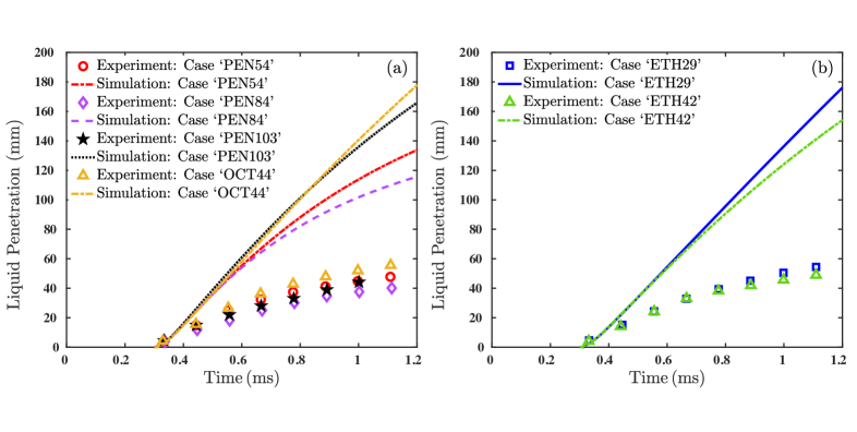
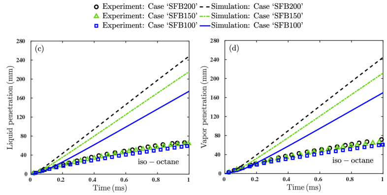
Figure 3: Comparison of the spray characteristics predicted by the CAS model without the model extensions and the experiments. Subfigures (a) & (b) show the comparison of liquid penetration lengths for the Aleiferis injector [Aleiferis and van Romunde, 2013] under different operating conditions for three different fuels, whereas subfigures (c) & (d) illustrate the comparison of liquid and vapor penetration lengths of iso-octane fuel, respectively, at different injection pressures for the ECN Spray G injector [Duronio et al., 2021].

5.2 Results with model extensions

This section discusses the gradual enhancements made in the previous CAS model performance, highlighting the inclusion or substitution of the new sub-models, as described in Section 2.

5.2.1 Spray cone angle and initial droplet size models

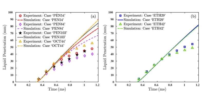
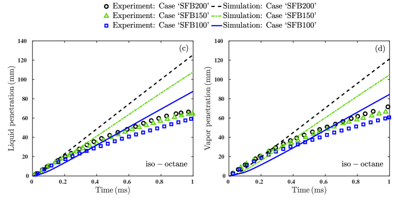
Figure 4: Spray characteristics predicted by the CAS model with updated spray cone angle (Eq. (13)) and initial droplet size (Eq. (44)) models. Subfigures (a) & (b) describe the comparison of liquid penetration lengths for the Aleiferis injector [Aleiferis and van Romunde, 2013] under different operating conditions for three different fuels, whereas subfigures (c) & (d) illustrate the comparison of liquid and vapor penetration lengths of iso-octane fuel, respectively, at different injection pressures for the ECN Spray G injector [Duronio et al., 2021].

Flash-boiling sprays are characterized by a widening of the spray plume due to the increased radial expansion resulting from the bubble growth and micro-explosion [Price et al., 2018]. Thus, accurate predictions of the spray cone angle as well as the initial droplet diameter play a crucial role in determining the global spray characteristics. Fig. 4 shows the CAS model performance with the upgraded models for spray cone angle (Eq. (13)) and initial droplet size (Eq. (44)) in comparison with the previous version during flash-boiling conditions. Here, the droplet heat transfer and vaporization processes are modeled via the standard Miller and Bellan model. For the droplet breakup, only KH–RT breakup model is incorporated. The gas phase temperature is obtained via the approach considered by Deshmukh et al. [2022b]. It is observed from Fig. 4 that the predictive capabilities of the CAS model are significantly improved with the updated cone angle and initial droplet diameter models compared to the previous version. However, the penetration lengths are quantitatively still overpredicted compared to the experimental measurements.

5.2.2 Superheated droplet vaporization, heat transfer, and breakup models

This section concludes the extension of the CAS model with the upgrade of the standard evaporation, heat transfer, and breakup models to that of the superheated vaporization, heat transfer, and hybrid aerodynamic-thermal breakup models, as described in Section 2. Here, Eq. (4) is incorporated for the calculation of the gas phase temperature. The improvements in the spray characteristics obtained from the fully updated CAS model are shown in Fig. 5 for different fuels under varying superheating degrees for the Aleiferis injector.

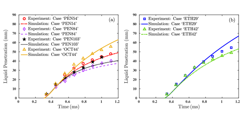
Figure 5: Spray characteristics predicted by the upgraded CAS model. Subfigures (a) & (b) describe the comparison of liquid penetration lengths for the Aleiferis injector [Aleiferis and van Romunde, 2013] for three different fuels under different operating conditions, as listed in Table 5.

Fig. 5a shows that the predicted spray penetration decreases with increasing $T_{\mathrm{inj}}$, from 363.15 K (case ‘PEN54’) to 393.15 K (case ‘PEN84’), at constant $P_{\mathrm{g}}=1.0$ bar for n-pentane fuel, as observed in the experiments. The increase in $T_{\mathrm{inj}}$ leads to an increase in liquid superheating degree ($\Delta T$) for the case ‘PEN84’, thus enhancing the evaporation rate and thermally induced breakup [Yang et al., 2013], which in turn produces the smaller droplets. These droplets then substantially decelerate due to the aerodynamic drag forces of the ambient gas, resulting in shorter spray penetrations. A similar trend is observed for flash-boiling ethanol (case ‘ETH29’ and ‘ETH42’), as illustrated in Fig. 5b.

With the system pressure $P_{\mathrm{g}}$, decreasing from 1.0 bar (case ‘PEN84’) to 0.5 bar (case ‘PEN103’), at $T_{\mathrm{inj}}=393.15$ K for n-pentane fuel, Fig. 5a shows that the predicted penetration length increases, as also reported in the experimental findings by Aleiferis and van Romunde [2013]. Table 5 shows that decreasing the system pressure for these n-pentane test cases leads to an increase in $\Delta T$ from 84 K to 103 K. The reason behind this phenomenon is the lower saturation temperature of the liquid under reduced pressure conditions. As described above, the liquid at higher $\Delta T$ is associated with increased evaporation and enhanced atomization effects, thus expected to result in smaller spray droplets and eventually shorter spray penetrations compared to the case with lower $\Delta T$. However, the resulting opposite trend in penetrations for these n-pentane test cases can be attributed to the lower system pressures. By lowering the pressures, the reduced aerodynamic drag forces are likely to outweigh the enhanced evaporation and atomization effects at high $\Delta T$, leading to an increase in penetration lengths. The predicted penetration length for iso-octane fuel at $\Delta T=44$ K (case ‘OCT44’) also agrees well with the experiment, as shown in Fig. 5a. Overall, the present CAS model is able to predict the trends in macroscopic spray characteristics similar to the experiments for different fuel properties and operating conditions for a given injector.

Fig. 6 depicts the improved spray characteristics of the ECN Spray G injector for varying injection pressures at a constant $R_{\mathrm{p}}$ of 0.26. The decreasing injection pressure leads to a reduction in the mass flow rate and subsequently, the residence time within the nozzle hole will be increased. Due to the longer residence time, the vapor bubbles start nucleating inside the injector nozzle leading to the formation of a well-atomized spray with a shorter penetration length. It is observed that the extended CAS model is able to predict the decreasing trend of spray penetrations with decreasing injection pressures, as also observed in the experiments.

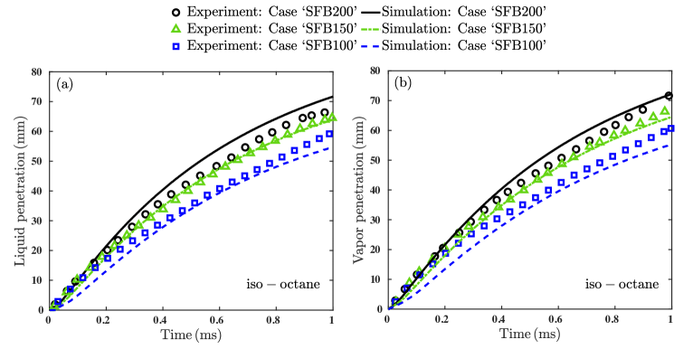
Figure 6: Spray characteristics predicted by the upgraded CAS model. Subfigures (a) & (b) illustrate the comparison of liquid and vapor penetration lengths of iso-octane fuel, respectively, for the ECN Spray G injector [Duronio et al., 2021] at different injection pressures, as listed in Table 5.

However, quantitatively, for some test cases, the present CAS model still over- and/or under-predicts the penetration lengths for both injectors. Although this is expected due to the averaged approach of the CAS model, the use of more accurate models for calculating the spray cone angle and initial droplet diameter is expected to improve the prediction towards the experiments vastly. This is because the increased radial expansion resulting from the bubble growth and micro-explosion would widen the spray plume as well as reduce initial droplet sizes under flash-boiling conditions [Price et al., 2018]. For a multi-hole injector, the wider spray plumes emerging from different injector holes could easily merge with each other depending on the inter-spacing and directions of the holes, thus resulting in even higher total plume widening compared to a single-hole injector. The present CAS model would not be able to capture the shattering of the child droplets due to micro-explosion and subsequent widening of the spray plume and reduced droplet sizes because of the continuous breakup approach considered. Thus, the spray cone angle and the initial droplet size models used in this study play a crucial role to mimic the above-mentioned phenomena. The influence of $\theta$ and $\mathsf{D_{o}}$ on the penetration length is illustrated in Fig. 7a and Fig. 7b for un-collapsed (case ‘ETH-29’) and collapsed (case ‘PEN103’) sprays, respectively. It can be seen that the reduced initial droplet size and higher spray cone angle improve the quantitative prediction of liquid penetration for the un-collapsed spray, whereas the increased droplet diameter associated with higher spray cone angle provides a more reasonable prediction of the liquid penetration length for the fully collapsed spray.

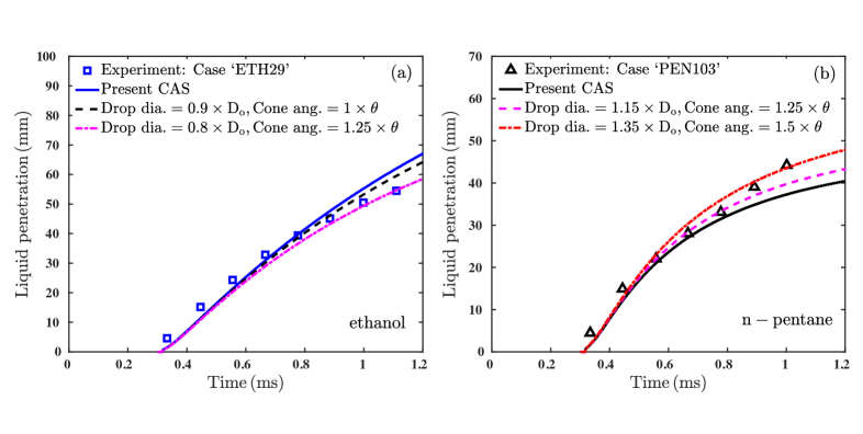
Figure 7: Influence of the spray cone angle and initial droplet diameter on the liquid penetration for (a) un-collapsed and (b) collapsed sprays of ethanol and n-pentane fuels, respectively.

5.3 Computational cost

In order to investigate the cost reduction factor associated with using the CAS model in comparison to the 3D simulations, an LES of flash-boiling spray is performed for case ‘PEN54’. A brief description of the numerical solver used for LES and the simulation results are included in C. Both the 1D and 3D simulations were run on machines that use the Intel Broadwell processor architecture. The 3D LES was run on 240 cores for $\approx$ 16.7 h leading to a total of 4008 CPUh. The 1D CAS was run on the same machine on 1 core for $\approx$ 205 s resulting in a total of 0.057 CPUh. Thus, the CAS model is faster by up to 4 orders of magnitude compared to the 3D LES while providing reasonable predictions in flash-boiling spray characteristics such as liquid and vapor penetration lengths for different operating conditions and fuels.

6 Conclusions

A reduced-order cross-sectionally averaged flash-boiling spray model was proposed in this work. The main conclusions of the present study can be summarized as follows:

• The previously developed CAS model was first applied to predict the spray characteristics such as penetration lengths for different fuels under flash-boiling conditions. It was found that the CAS model fails to reproduce the trend in the flash-boiling spray penetration lengths.

• An extension of the CAS model was then proposed to improve its predictive capabilities for the simulation of flash-boiling sprays. The important physical subprocesses in flash-boiling sprays such as internal vaporization, external vaporization, and thermally driven breakup were incorporated into the newly developed CAS model. The initial droplet diameter for flash-boiling sprays, which is expected to be considerably smaller than the nozzle exit diameter, was estimated using an experimental correlation available in the literature. Additionally, an appropriate empirical formulation was employed to model the wider spray plume angle observed in flash-boiling conditions

• The upgraded CAS model performance was compared with the experimental measurements of two different injector nozzles for varying injection pressures and superheating degrees. It was found that the trends in liquid and vapor penetration lengths predicted by the updated CAS model agree well with the experiments.

• Though in some cases, the penetration lengths were found to be under-and/or over-predicted due to the averaged approach of the CAS model, it was shown that the prediction could be improved with the more accurate modeling of the spray cone angle and initial droplet diameter.

• A 3D LES of a flash-boiling spray was also performed in order to assess the computational efficiency of the CAS model. The 1D CAS model was shown to be faster by up to four orders of magnitude in comparison to the 3D LES, thus making it really useful in many practical applications related to flash-boiling including but not limited to the design of experiments, rapid fuel-screening, and creating digital twins.

Appendix A Derivation of the superheated vaporization coefficients

subsectionInternal Vaporization The vaporization of the superheated liquid causes the vapor bubbles to grow in size and subsequently leads to the expansion of the liquid droplet. For a single bubble, from the mass continuity

$$\rho_{\mathrm{l}}\frac{\text{d}R_{\text{d}}}{\text{d}t}=\rho_{\text{v}}\frac{\text{d}R_{\text{b}}}{\text{d}t}.$$ (46)

Rearranging 46 yields

$$\frac{\text{d}d^{2}_{\text{d}}}{\text{d}t}=4d_{\text{d}}\frac{\rho_{\text{v}}}{\rho_{\mathrm{l}}}\frac{\text{d}R_{\text{b}}}{\text{d}t}.$$ (47)

Summing over the total number of vapor bubbles, 47 becomes

$$\frac{\text{d}d^{2}_{\text{d}}}{\text{d}t}=N_{\mathrm{bub}}\times 4d_{\text{d}}\frac{\rho_{\text{v}}}{\rho_{\mathrm{l}}}\frac{\text{d}R_{\text{.}}pdfb}{\text{d}t}=K_{\mathrm{vap,exp}}$$ (48)

A.1 External Vaporization

The vapor mass flux from the droplet outer surface due to the heat transfer from the droplet inner core is modeled as [Adachi et al., 1997]

$$\rho_{\text{s}}v_{\text{s}}=\frac{h_{\text{f}}\left(T_{\mathrm{d}}-{T_{\mathrm{b}}}\right)}{L\left({T_{\mathrm{b}}}\right)},$$ (49)

where $v_{\mathrm{s}}$ denotes the vapor flow rate from the droplet outer surface. From the mass continuity at the droplet surface

$$\frac{\rho_{\mathrm{l}}}{2}\frac{\mathrm{d}{d_{\mathrm{d}}}}{\mathrm{d}t}=\rho_{\text{s}}v_{\text{s}}.$$ (50)

Equating Eq. (50) with the Eq. (49) yields

$$\frac{\rho_{\mathrm{l}}}{2}\frac{\mathrm{d}{d_{\mathrm{d}}}}{\mathrm{d}t}=\frac{h_{\text{f}}\left(T_{\mathrm{d}}-{T_{\mathrm{b}}}\right)}{L\left({T_{\mathrm{b}}}\right)}.$$ (51)

Rearranging Eq. (51), the rate of change of ${d}^{2}_{\mathrm{d}}$ can be expressed as

$$\frac{\mathrm{d}{d}^{2}_{\mathrm{d}}}{\mathrm{d}t}=\frac{4{d_{\mathrm{d}}}h_{\text{f}}\left(T_{\mathrm{d}}-{T_{\mathrm{b}}}\right)}{\rho_{\mathrm{l}}L\left({T_{\mathrm{b}}}\right)}=K_{\mathrm{vap,ht1}}.$$ (52)

Similarly, the vapor mass flux due to the temperature gradient between the droplet surface and the external ambient is expressed as

$$\rho_{s}v_{s}=\frac{h_{\text{ex}}f_{3}\left|{T_{\mathrm{g}}}-{T_{\mathrm{s}}}\right|}{L\left({T_{\mathrm{s}}}\right)}.$$ (53)

Using mass continuity at the droplet surface (Eq. (50)) and rearranging Eq. (53) yields

$$\frac{\mathrm{d}{d}^{2}_{\mathrm{d}}}{\mathrm{d}t}=\frac{4{d_{\mathrm{d}}}f_{3}h_{\mathrm{ex}}\left|{T_{\mathrm{g}}}-{T_{\mathrm{s}}}\right|}{\rho_{\mathrm{l}}L\left({T_{\mathrm{s}}}\right)}=K_{\mathrm{vap,ht2}}.$$ (54)

Appendix B Derivation of the heat transfer coefficient

The energy balance of the droplet-bubble system in the superheated regime can be written as

$$m_{\text{d}}C_{\text{l}}\left(T_{\mathrm{d}}\right)\frac{\mathrm{d}T_{\mathrm{d}}}{\mathrm{d}t}=4\pi r^{2}_{\text{d}}Q_{\text{d}}-4\pi r^{2}_{\text{d}}\rho_{\text{s}}v_{\text{s}}L\left({T_{\mathrm{s}}}\right)-4\pi R^{2}_{\text{b}}\rho_{\mathrm{v}}N_{\mathrm{bub}}\dot{R}_{\text{b}}L\left(T_{\mathrm{d}}\right).$$ (55)

Substituting

$$Q_{\mathrm{d}}=\frac{\lambda_{\mathrm{g}}\left(T_{\mathrm{ref}}\right)\left({T_{\mathrm{g}}}-{T_{\mathrm{s}}}\right)}{{{d_{\mathrm{d}}}}}f_{\text{2,sup}}\mathsf{Nu_{\mathrm{{d}}}}$$ (56)

and

$$\rho_{s}v_{s}=\frac{h_{\text{f}}\left(T_{\mathrm{d}}-{T_{\mathrm{b}}}\right)}{L\left({T_{\mathrm{b}}}\right)}+\frac{f_{3}h_{\text{ex}}|{T_{\mathrm{g}}}-{T_{\mathrm{s}}}|}{L\left({T_{\mathrm{b}}}\right)}$$ (57)

in Eq. (55) and rearranging yields

$$\frac{\text{d}T_{\mathrm{d}}}{\text{d}t}=\frac{6f_{\text{2,sup}}\mathsf{Nu_{\mathrm{{d}}}}\lambda_{\mathrm{g}}(T_{\mathrm{ref}})({T_{\mathrm{g}}}-{T_{\mathrm{s}}})}{\rho_{\mathrm{l}}{d}^{2}_{\mathrm{d}}C_{\mathrm{p,\mathrm{l}}}(T_{\mathrm{d}})}-\frac{3K_{\mathrm{vap,ext}}L\left({T_{\mathrm{s}}}\right)}{2d^{2}_{\text{d}}C_{\text{l}}\left(T_{\mathrm{d}}\right)}-\frac{3K_{\mathrm{vap,exp}}L\left(T_{\mathrm{d}}\right)}{2d^{2}_{\text{d}}C_{\text{l}}\left(T_{\mathrm{d}}\right)}=K_{\mathrm{heat}}.$$ (58)

The energy balance of the droplet-bubble system in the subcooled regime can be written as

$$m_{\text{d}}C_{\text{l}}\left(T_{\mathrm{d}}\right)\frac{\mathrm{d}T_{\mathrm{d}}}{\mathrm{d}t}=4\pi r^{2}_{\text{d}}Q_{\text{d}}-4\pi r^{2}_{\text{d}}\rho_{\text{s}}v_{\text{s}}L\left({T_{\mathrm{s}}}\right).$$ (59)

Substituting

$$Q_{\mathrm{d}}=\frac{\lambda_{\mathrm{g}}\left(T_{\mathrm{ref}}\right)\left({T_{\mathrm{g}}}-{T_{\mathrm{s}}}\right)}{{{d_{\mathrm{d}}}}}f_{\text{2,sub}}\mathsf{Nu_{\mathrm{{d}}}}\hskip 14.22636pt\text{and}\hskip 14.22636pt\rho_{\text{s}}v_{\text{s}}=2\rho_{\text{s}}\Gamma_{\text{v,g}}\frac{ln(1+B_{\text{M,d}})}{d_{\text{d}}}$$ (60)

in Eq. (59) and rearranging yields

$$\frac{\mathrm{d}T_{\mathrm{d}}}{\mathrm{d}t}=\frac{6f_{\text{2,sub}}\mathsf{Nu_{\mathrm{{d}}}}\lambda_{\mathrm{g}}(T_{\mathrm{ref}})({T_{\mathrm{g}}}-{T_{\mathrm{s}}})}{\rho_{\mathrm{l}}{d}^{2}_{\mathrm{d}}C_{\mathrm{p,\mathrm{l}}}(T_{\mathrm{d}})}-\frac{3K_{\mathrm{vap,ext}}L\left({T_{\mathrm{s}}}\right)}{2d^{2}_{\text{d}}C_{\text{l}}\left(T_{\mathrm{d}}\right)}=K_{\mathrm{heat}}.$$ (61)

Appendix C LES of flash-boiling spray

An LES of a flash-boiling spray is performed using a two-way coupled 3D Lagrangian-Eulerian framework. The in-house code CIAO is used to solve the compressible Navier-Stokes equations (NSEs). CIAO is a structured, high-order, finite-difference code, which solves the NSEs using central difference schemes. For time-marching, CIAO uses a low-storage five-stage, explicit Runge-Kutta (RK) scheme. The subgrid stresses are modeled using a dynamic Smagorinski subfilter model considering Lagrangian averaging Germano et al. [1991]. For more details about the flow solver in CIAO, the reader is referred to Mittal et al. [2014]. For the computation of the dispersed liquid phase, the Lagrangian equations governing the single droplet position, velocity, mass, and temperature are solved Miller and Bellan [1999]. Both the internal and external vaporization processes of the superheated droplets are considered. The newly developed semi-analytical solution for bubble growth rate by Saha et al. [2023] is incorporated to obtain the bubble growth dynamics in the superheated droplets. Due to the smaller size of the droplets in flash-boiling sprays, the conductive thermal resistance in the superheated liquid droplets is neglected and the droplet bulk temperature is modeled using an infinite conductivity model [Miller and Bellan, 1999]. The vapor contained in the bubbles is assumed to be in equilibrium with the surrounding superheated liquid medium. A hybrid breakup model consisting of flash-boiling induced breakup [Senda et al., 1994] and aerodynamic breakup [Patterson and Reitz, 1998] is incorporated to simulate the breakup process under superheated conditions.

The LES is performed on a structured grid with a cell size of 180 $\mu$m resulting in a total cell count of 8.45 million. The simulation results are compared with the experiments in terms of the penetration length and the steady-state Sauter-mean diameter (SMD). Fig. 8 shows the comparison of the liquid penetration lengths obtained from the LES and the experimental measurements of Aleiferis and van Romunde [2013] for n-pentane fuel at $P_{\mathrm{inj}}=150$ bar, $P_{\mathrm{g}}=1.0$ bar, and $T_{\mathrm{inj}}=363.15$ K.

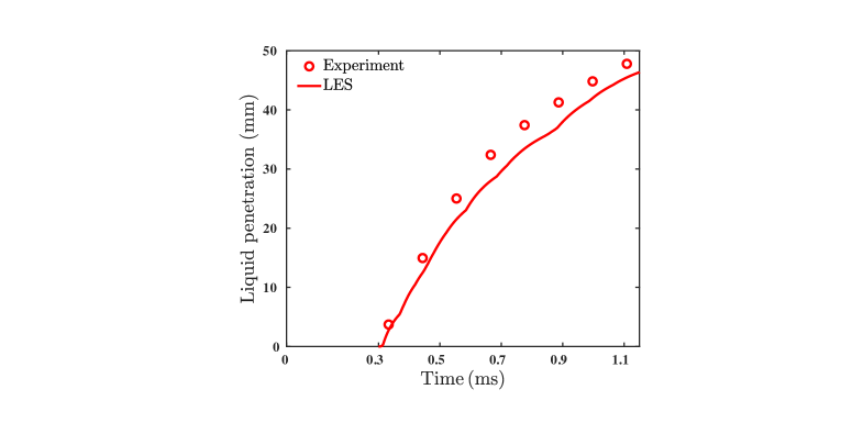
Figure 8: Comparison of the liquid penetration length of n-pentane fuel at $P_{\mathrm{inj}}=150$ bar, $P_{\mathrm{g}}=1.0$ bar, and $T_{\mathrm{inj}}=363.15$ K. Experimental measurements are taken from Aleiferis and van Romunde [2013].

Considering the complexity of flash-boiling modeling, the spray penetration length obtained from the LES shows reasonable agreement with the experiment. A steady-state SMD value of 7.6 $\mu$m is obtained from the LES, which is also found to be within a few microns of the experimentally measured value of 7.9 $\mu$m. The SMD was measured using a Laser diffraction technique at 30 mm along the injector central axis downstream of the nozzle exit in the experiment.

Appendix D Availability of the code

The FORTRAN90 code framework is made open-source and can be found here: https://git.rwth-aachen.de/avijitsaha021/cross-sectionally-averaged-spray-model/

References

- Adachi et al. [1997] Adachi, M., McDonell, V.G., Tanaka, D., Senda, J., Fujimoto, H., 1997. Characterization of fuel vapor concentration inside a flash boiling spray, in: International Congress & Exposition, SAE International. doi:https://doi.org/10.4271/970871.
- Aleiferis et al. [2010a] Aleiferis, P., Serras-Pereira, J., Augoye, A., Davies, T.J., Cracknell, R.F., Richardson, D., 2010a. Effect of fuel temperature on in-nozzle cavitation and spray formation of liquid hydrocarbons and alcohols from a real-size optical injector for direct-injection spark-ignition engines. International Journal of Heat and Mass Transfer 53, 4588–4606. doi:10.1016/j.ijheatmasstransfer.2010.06.033.
- Aleiferis et al. [2010b] Aleiferis, P., Serras-Pereira, J., van Romunde, Z., Caine, J., Wirth, M., 2010b. Mechanisms of spray formation and combustion from a multi-hole injector with e85 and gasoline. Combustion and Flame 157, 735–756. doi:https://doi.org/10.1016/j.combustflame.2009.12.019.
- Aleiferis and van Romunde [2013] Aleiferis, P., van Romunde, Z.R., 2013. An analysis of spray development with iso-octane, n-pentane, gasoline, ethanol and n-butanol from a multi-hole injector under hot fuel conditions. Fuel 105, 143–168. doi:http://dx.doi.org/10.1016/j.fuel.2012.07.044.
- Badawy et al. [2022] Badawy, T., Xu, H., Li, Y., 2022. Macroscopic spray characteristics of iso-octane, ethanol, gasoline and methanol from a multi-hole injector under flash boiling conditions. Fuel 307, 121820. doi:https://doi.org/10.1016/j.fuel.2021.121820.
- Brown and York [1962] Brown, R., York, J., 1962. Sprays formed by flashing liquid jets. AIChE Journal 8, 149–53.
- CMT [2023] CMT, 2023. Virtual injection rate generator, CMT-Motores Tér micos, Universitat Politècnica de València. URL: https://www.cmt.upv.es/. Accessed on 21.03.2023.
- Crowe et al. [2012] Crowe, C.T., Schwarzkopf, J.D., Sommerfeld, M., Tsuji, Y., 2012. Mulitphase Flows with Droplets and Particles. Taylor & Francis Group, LLC.
- Desantes et al. [2009] Desantes, J., Pastor, J., García-Oliver, J., Pastor, J., 2009. A 1D model for the description of mixing-controlled reacting diesel sprays. Combustion and Flame 156, 234–249. doi:10.1016/j.combustflame.2008.10.008.
- Desantes et al. [2006] Desantes, J.M., Payri, R., Salvador, F.J., Gil, A., 2006. Development and validation of a theoretical model for diesel spray penetration. Fuel 22, 87–110. doi:10.1016/j.fuel.2005.10.023.
- Deshmukh et al. [2022a] Deshmukh, A.Y., Davidovic, M., Grenga, T., Lakshmanan, R., Cai, L., Pitsch, H., 2022a. A reduced-order model for turbulent reactive sprays in compression ignition engines. Combustion and Flame 236, 111751. doi:https://doi.org/10.1016/j.combustflame.2021.111751.
- Deshmukh et al. [2022b] Deshmukh, A.Y., Grenga, T., Davidovic, M., Schumacher, L., Palmer, J., Reddemann, M.A., Kneer, R., Pitsch, H., 2022b. A reduced-order model for multiphase simulation of transient inert sprays. Internation Journal of Multiphase Flows 147, 103872. doi:https://doi.org/10.1016/j.ijmultiphaseflow.2021.103872.
- Dietzel [2020] Dietzel, D.R., 2020. Modeling and simulation of flash-boiling of cryogenic liquids. Ph.D. thesis.
- Duronio et al. [2022] Duronio, F., Mascio, A.D., Villante, C., Anatone, M., Vita, A.D., 2022. Ecn spray g: Coupled eulerian internal nozzle flow and lagrangian spray simulation in flash boiling conditions. International Journal of Engine Research 0, 14680874221090732. doi:10.1177/14680874221090732.
- Duronio et al. [2021] Duronio, F., Ranieri, S., Montanaro, A., Allocca, L., De Vita, A., 2021. Ecn spray g injector: Numerical modelling of flash-boiling breakup and spray collapse. International Journal of Multiphase Flow 145, 103817. doi:https://doi.org/10.1016/j.ijmultiphaseflow.2021.103817.
- ECN [2020] ECN, 2020. Engine Combustion Network (ECN). URL: https://ecn.sandia.gov/. Accessed on 12.10.2020.
- Fujimoto et al. [1997] Fujimoto, H., Iwami, Y., Senda, J., 1997. Atomization Characteristics of Liquefied n-Butane Spray with Flash Boiling Phenomena. International Journal of Fluid Mechanics Research 24, 273–282. doi:10.1615/InterJFluidMechRes.v24.i1-3.270.
- Gemci et al. [2004] Gemci, T., Yakut, K., Chigier, N., Ho, T.C., 2004. Experimental study of flash atomization of binary hydrocarbon liquids. International Journal of Multiphase Flows 30, 395–417. doi:doi:10.1016/j.ijmultiphaseflow.2003.12.003.
- Germano et al. [1991] Germano, M., Piomelli, U., Moin, P., Cabot, W.H., 1991. A dynamic subgrid‐scale eddy viscosity model. Physics of Fluids A: Fluid Dynamics 3, 1760–1765. doi:10.1063/1.857955.
- Ghandilou and Taghavifar [2022] Ghandilou, A.J., Taghavifar, H., 2022. New insight into air/spray boundary interaction for diesel and biodiesel fuels under different fuel temperatures. Biofuels 13, 1087–1101. doi:https://doi.org/10.1080/17597269.2022.2105867.
- Guo et al. [2017a] Guo, H., Ding, H., Li, Y., Ma, X., Wang, Z., Xu, H., Wang, J., 2017a. Comparison of spray collapses at elevated ambient pressure and flash boiling conditions using multi-hole gasoline direct injector. Fuel 199, 125–134. doi:https://doi.org/10.1016/j.fuel.2017.02.071.
- Guo et al. [2019] Guo, H., Li, Y., Wang, B., Zhang, H., Xu, H., 2019. Numerical investigation on flashing jet behaviors of single-hole gdi injector. International Journal of Heat and Mass Transfer 130, 50–59. doi:https://doi.org/10.1016/j.ijheatmasstransfer.2018.10.088.
- Guo et al. [2017b] Guo, H., Ma, X., Li, Y., Liang, S., Wang, Z., Xu, H., Wang, J., 2017b. Effect of flash boiling on microscopic and macroscopic spray characteristics in optical gdi engine. Fuel 190, 79–89. doi:http://dx.doi.org/10.1016/j.fuel.2016.11.043.
- Guo et al. [2018] Guo, H., Wang, B., Li, Y., Xu, H., Wu, Z., 2018. Characterizing external flashing jet from single-hole gdi injector. International Journal of Heat and Mass Transfer 121, 924–932. doi:https://doi.org/10.1016/j.ijheatmasstransfer.2018.01.042.
- Hiroyasu and Arai [1980] Hiroyasu, H., Arai, M., 1980. Fuel spray penetration and spray angle of diesel engines. Trans. JSAE 21, 5–11.
- Hubbard et al. [1975] Hubbard, G., Denny, V., Mills, A., 1975. Droplet evaporation: Effects of transients and variable properties. International Journal of Heat and Mass Transfer 18, 1003–1008. doi:10.1016/0017-9310(75)90217-3.
- Kale and Banerjee [2019] Kale, R., Banerjee, R., 2019. Understanding spray and atomization characteristics of butanol isomers and isooctane under engine like hot injector body conditions. Fuel 237, 191–201. doi:https://doi.org/10.1016/j.fuel.2018.09.142.
- Kawano et al. [2004] Kawano, D., Goto, Y., Odaka, M., Senda, J., 2004. Modeling atomization and vaporization processes of flash-boiling spray, in: SAE 2004 World Congress & Exhibition, SAE International. doi:https://doi.org/10.4271/2004-01-0534.
- Leach et al. [2013] Leach, F., Stone, R., Fennell, D., Hayden, D., Richardson, D., Wicks, N., 2013. Internal Combustion Engines: Performance, Fuel Economy and Emissions. Woodhead Publishing, London. pp. 193–202. doi:https://doi.org/10.1533/9781782421849.5.193.
- Lefebvre [1988] Lefebvre, A.H., 1988. Atomization and Sprays. Hemisphere Publishing Cooperation, New York, USA.
- Li et al. [2017] Li, S., Zhang, Y., Qi, W., Xu, B., 2017. Quantitative observation on characteristics and breakup of single superheated droplet. Experimental Thermal and Fluid Science 80, 305–312. doi:https://doi.org/10.1016/j.expthermflusci.2016.09.004.
- Li et al. [2018a] Li, Y., Guo, H., Fei, S., Ma, X., Zhang, Z., Chen, L., Feng, L., Wang, Z., 2018a. An exploration on collapse mechanism of multi-jet flash-boiling sprays. Applied Thermal Engineering 134, 20–28. doi:https://doi.org/10.1016/j.applthermaleng.2018.01.102.
- Li et al. [2018b] Li, Y., Guo, H., Ma, X., Qi, Y., Wang, Z., Xu, H., Shuai, S., 2018b. Morphology analysis on multi-jet flash-boiling sprays under wide ambient pressures. Fuel 211, 38–47. doi:https://doi.org/10.1016/j.fuel.2017.08.082.
- Li et al. [2019] Li, Y., Guo, H., Zhou, Z., Zhang, Z., Ma, X., Chen, L., 2019. Spray morphology transformation of propane, n-hexane and iso-octane under flash-boiling conditions. Fuel 236, 677–685. doi:https://doi.org/10.1016/j.fuel.2018.08.160.
- Miller and Bellan [1999] Miller, R.S., Bellan, J., 1999. Direct numerical simulation of a confined three-dimensional gas mixing layer with one evaporating hydrocarbon-droplet-laden stream. Journal of Fluid Mechanics 384, 293–338. doi:10.1017/S0022112098004042.
- Mittal et al. [2014] Mittal, V., Kang, S., Doran, E., Cook, D., Pitsch, H., 2014. LES of Gas Exchange in IC Engines. Oil & Gas Science and Technology – Revue d’IFP Energies nouvelles 69, 29–40. doi:10.2516/ogst/2013122.
- Mojtabi et al. [2014] Mojtabi, M., Wigley, G., Helie, J., 2014. The effect of flash boiling on the atomization performance of gasoline direct injection multistream injectors. Atomization and Sprays 24, 467–493. doi:10.1615/AtomizSpr.2014008296.
- Pastor et al. [2008] Pastor, J.V., Javier Lopez, J., Garcia, J., Pastor, J.M., 2008. A 1D model for the description of mixing-controlled inert diesel sprays. Fuel 87, 2871–2885. doi:10.1016/j.fuel.2008.04.017.
- Patterson and Reitz [1998] Patterson, M.A., Reitz, R.D., 1998. Modeling the effects of fuel spray characteristics on diesel engine combustion and emission, in: International Congress & Exposition, SAE International. doi:https://doi.org/10.4271/980131.
- Pickett et al. [2011] Pickett, L.M., Manin, J., Genzale, C.L., Siebers, D.L., Musculus, M.P., Idicheria, C.A., 2011. Relationship Between Diesel Fuel Spray Vapor Penetration/Dispersion and Local Fuel Mixture Fraction. SAE International Journal of Engines doi:10.4271/2011-01-0686.
- Price et al. [2015] Price, C., Hamzehloo, A., Aleiferis, P., Richardson, D., 2015. Aspects of numerical modelling of flash-boiling fuel sprays, in: 12th International Conference on Engines & Vehicles, SAE International. doi:https://doi.org/10.4271/2015-24-2463.
- Price et al. [2016] Price, C., Hamzehloo, A., Aleiferis, P., Richardson, D., 2016. An Approach to Modeling Flash-Boiling Fuel Sprays for Direct-injection Spark-ignition Engines. Atomization and Sprays 26, 1–43. doi:10.1615/AtomizSpr.2016015807.
- Price et al. [2018] Price, C., Hamzehloo, A., Aleiferis, P., Richardson, D., 2018. Numerical modelling of fuel spray formation and collapse from multi-hole injectors under flash-boiling conditions. Fuel 221, 518–541. doi:10.1016/j.fuel.2018.01.088.
- Price et al. [2020] Price, C., Hamzehloo, A., Aleiferis, P., Richardson, D., 2020. Numerical modelling of droplet breakup for flash-boiling fuel spray predictions. International Journal of Multiphase Flow 125, 103183. doi:https://doi.org/10.1016/j.ijmultiphaseflow.2019.103183.
- Ranz and Marshall [1952] Ranz, W.E., Marshall, W.R., 1952. Evaporation from drops. Parts I & II. Chem. Eng. Progr 48, 141–146; 173–180. doi:10.1016/S0924-7963(01)00032-X.
- Ratcliff et al. [2016] Ratcliff, M.A., Burton, J., Sindler, P., Christensen, E., Fouts, L., Chupka, G.M., McCormick, R.L., 2016. Knock resistance and fine particle emissions for several biomass-derived oxygenates in a direct-injection spark-ignition engine. SAE International Journal of Fuels and Lubricants 9, 59–70. URL: https://doi.org/10.4271/2016-01-0705, doi:https://doi.org/10.4271/2016-01-0705.
- Reitz [1987] Reitz, R.D., 1987. Modeling Atomization Processes in High-Pressure Vaporizing Sprays. Atomization and Sprays 3, 309–337.
- Reitz [2013] Reitz, R.D., 2013. Directions in internal combustion engine research. Combustion and Flame 160, 1–8. doi:https://doi.org/10.1016/j.combustflame.2012.11.002.
- Reitz and Diwakar [1987] Reitz, R.D., Diwakar, R., 1987. Structure of high-pressure fuel sprays, in: SAE International Congress and Exposition, SAE International. doi:https://doi.org/10.4271/870598.
- Rusanov [1961] Rusanov, V.V., 1961. Calculation of interaction of non–steady shock waves with obstacles. J. Comput. Math. Phys. USSR .
- Saha et al. [2021] Saha, A., Deshmukh, A.Y., Grenga, T., Bode, M., Grunewald, M., Kaya, Y., Kirsch, V., Reddemann, M.A., Kneer, R., Pitsch, H., 2021. Numerical Modeling of the Flash Boiling Characteristics of E-Fuels at Low Ambient Pressure, in: International Conference on Liquid Atomization and Spray Systems (ICLASS), 30th September - 2nd September, Edinburgh, Scotland UK.
- Saha et al. [2023] Saha, A., Deshmukh, A.Y., Grenga, T., Pitsch, H., 2023. Dimensional analysis of vapor bubble growth considering bubble-bubble interactions in flash boiling microdroplets of highly volatile liquid electrofuels. International Journal of Multiphase Flow 165, 104479. doi:https://doi.org/10.1016/j.ijmultiphaseflow.2023.104479.
- Saha et al. [2022] Saha, A., Grenga, T., Deshmukh, A.Y., Hinrichs, J., Bode, M., Pitsch, H., 2022. Numerical modeling of single droplet flash boiling behavior of e-fuels considering internal and external vaporization. Fuel 308, 121934.
- Sazhin et al. [2001] Sazhin, S., Feng, G., Heikal, M., 2001. A model for fuel spray penetration. Fuel 80, 2171–2180. doi:10.1016/S0016-2361(01)00098-9.
- Schmitz et al. [2002] Schmitz, I., Ipp, W., Leipertz, A., 2002. Flash Boiling Effects on the Development of Gasoline Direct-Injection Engine Sprays. SAE Journal of Fuels and Lubricants 111, 1025–1032. URL: https://www.jstor.org/stable/44734585.
- Senda et al. [1994] Senda, J., Hojyo, Y., Fujimoto, H., 1994. Modelling of atomization process in flash boiling spray, in: International Fuels & Lubricants Meeting & Exposition, SAE International. doi:https://doi.org/10.4271/941925.
- Senda et al. [2008] Senda, J., Wada, Y., Kawano, D., Fujimoto, H., 2008. Improvement of combustion and emissions indiesel engines by means of enhanced mixtureformation based on flash boiling of mixed fuel. International Journal of Engine Research 9, 15–27. doi:10.1243/14680874JER02007.
- Serras-Pereira et al. [2010] Serras-Pereira, J., van Romunde, Z., Aleiferis, P., Richardson, D., Wallace, S., Cracknell, R.F., 2010. Cavitation, primary break-up and flash boiling of gasoline, iso-octane and n-pentane with a real-size optical direct-injection nozzle. Fuel 89, 2592–2607. doi:https://doi.org/10.1016/j.fuel.2010.03.030.
- She [2010] She, J., 2010. Experimental study on improvement of diesel combustion and emissions using flash boiling injection, in: SAE 2010 World Congress & Exhibition, SAE International. URL: https://doi.org/10.4271/2010-01-0341, doi:https://doi.org/10.4271/2010-01-0341.
- Sher and Elata [1977] Sher, E., Elata, C., 1977. Spray Formation from Pressure Cans by Flashing. Ind. Eng. Chem., Process Des. Dev. 16, 237–242. doi:https://doi.org/10.1021/i260062a014.
- Siebers [1999] Siebers, D.L., 1999. Scaling liquid-phase fuel penetration in diesel sprays based on mixing-limited vaporization. SAE Technical Paper 1999-01-0528 doi:10.4271/1999-01-0528.
- Sun et al. [2021a] Sun, Z., Cui, M., Nour, M., Li, X., Hung, D., Xu, M., 2021a. Study of flash boiling combustion with different fuel injection timings in an optical engine using digital image processing diagnostics. Fuel 284, 119078. doi:https://doi.org/10.1016/j.fuel.2020.119078.
- Sun et al. [2021b] Sun, Z., Cui, M., Ye, C., Yang, S., Li, X., Hung, D., Xu, M., 2021b. Split injection flash boiling spray for high efficiency and low emissions in a gdi engine under lean combustion condition. Proceedings of the Combustion Institute 38, 5769–5779. doi:https://doi.org/10.1016/j.proci.2020.05.037.
- Sun et al. [2020] Sun, Z., Yang, S., Nour, M., Li, X., Hung, D., Xu, M., 2020. Significant impact of flash boiling spray on in-cylinder soot formation and oxidation process. Energy Fuels 34, 10030–10038. doi:https://doi.org/10.1021/acs.energyfuels.0c01942.
- Vanderwege and Hochgreb [1998] Vanderwege, B.A., Hochgreb, S., 1998. The effect of fuel volatility on sprays from high-pressure swirl injectors. Symposium (International) on Combustion 27, 1865–1871. doi:https://doi.org/10.1016/S0082-0784(98)80029-5.
- von Kuensberg Sarre et al. [1999] von Kuensberg Sarre, C., Kong, S.c., Reitz, R.D., 1999. Modeling the Effects of Injector Nozzle Geometry on Diesel Sprays. SAE Technical Paper 1999-01-0912 , 1–14doi:10.4271/1999-01-0912.
- Wallis [1969] Wallis, G.B., 1969. One-Dimensional Two-Phase Flow. McGraw-Hill, New York.
- Wan [1997] Wan, Y., 1997. Numerical Study of Transient Fuel Sprays with Autoignition and Combustion Under Diesel-Engine Relevant Conditions. Ph.D. thesis. RWTH Aachen University.
- Wang et al. [2020] Wang, J., Qiao, X., Ju, D., Sun, C., Wang, T., 2020. Bubble nucleation, micro-explosion and residue formation in superheated jatropha oil droplet: The phenomena of vapor plume and vapor cloud. Fuel 261, 116431. URL: https://www.sciencedirect.com/science/article/pii/S0016236119317855, doi:https://doi.org/10.1016/j.fuel.2019.116431.
- Wang et al. [2017a] Wang, Z., Badawy, T., Wang, B., Jiang, Y., Xu, H., 2017a. Experimental characterization of closely coupled split isooctane sprays under flash boiling conditions. Applied Energy 193, 199–209. doi:https://doi.org/10.1016/j.apenergy.2017.02.009.
- Wang et al. [2017b] Wang, Z., Liu, H., Reitz, R.D., 2017b. Knocking combustion in spark-ignition engines. Progress in Energy and Combustion Science 61, 78–112. doi:https://doi.org/10.1016/j.pecs.2017.03.004.
- Wang et al. [2017c] Wang, Z., Ma, X., Jiang, Y., Li, Y., Xu, H., 2017c. Influence of deposit on spray behaviour under flash boiling condition with the application of closely coupled split injection strategy. Fuel 190, 67–78. doi:https://doi.org/10.1016/j.fuel.2016.11.012.
- Wilke [1950] Wilke, C.R., 1950. A viscosity equation for gas mixtures. The Journal of Chemical Physics 18, 517. doi:10.1063/1.1747673.
- Xi et al. [2017] Xi, X., Liu, H., Jia, M., Xie, M., Yin, H., 2017. A new flash boiling model for single droplet. Fuel 107, 1129–1137. doi:10.1016/j.ijheatmasstransfer.2016.11.027.
- Xu et al. [2013] Xu, M., Zhang, Y., Zeng, W., Zhang, G., Zhang, M., 2013. Flash Boiling: Easy and Better Way to Generate Ideal Sprays than the High Injection Pressure. SAE International Journal of Fuels and Lubricants 6, 137–148. doi:10.4271/2013-01-1614.
- Yamazaki et al. [1985] Yamazaki, N., Miyamoto, N., Murayama, T., 1985. The Effects of Flash Boiling Fuel Injection on Spray Characteristics, Combustion, and Engine Performance in DI and IDI Diesel Engines. SAE Transactions 94, 388–395. URL: https://www.jstor.org/stable/44467680.
- Yang [2017] Yang, S., 2017. Development and validation of a flash boiling model for single-component fuel droplets. Atomization and Sprays 27, 963–997. doi:10.1615/AtomizSpr.2017020237.
- Yang et al. [2013] Yang, S., Song, Z., Wang, T., Yao, Z., 2013. An experimental study on phenomenon and mechanism of flash boiling spray from a multi-hole gasoline direct injector. Atomization and Sprays 23, 379–399. doi:10.1615/AtomizSpr.2013007539.
- Zeng et al. [2012] Zeng, W., Xu, M., Zhang, G., Zhang, Y., Cleary, D.J., 2012. Atomization and vaporization for flash-boiling multi-hole sprays with alcohol fuels. Fuel 95, 287–297. doi:10.1016/j.fuel.2011.08.048.
- Zeng and Lee [2001] Zeng, Y., Lee, C.F.F., 2001. An Atomization Model For Flash Boiling Sprays. Combustion Science and Technology 169, 45–67. doi:http://dx.doi.org/10.1080/00102200108907839.
- Zhao [2010] Zhao, H., 2010. Advanced Direct Injection Combustion Engine Technologies and Development: Gasoline and Gas Engines. Cambridge: Woodhead.
- Zhao [2021] Zhao, Z., 2021. High injection pressure impinging diesel spray characteristics and subsequent soot formation in reacting conditions. Ph.D. thesis. Michigan Technical University. doi:https://doi.org/10.37099/mtu.dc.etdr/1318.
- Zhou et al. [2018] Zhou, Z.F., Lu, G.Y., Chen, B., 2018. Numerical study on the spray and thermal characteristics of r404a flashing spray using openfoam. International Journal of Heat and Mass Transfer 117, 1312–1321. doi:https://doi.org/10.1016/j.ijheatmasstransfer.2017.10.095.
- Zuo et al. [2000] Zuo, B., Gomes, A.M., Rutland, C.J., 2000. Modelling superheated fuel sprays and vaproization. International Journal of Engine Research 1, 321–336. doi:10.1243/1468087001545218.