Exact recovery of the support of piecewise constant images via total variation regularization

Abstract

This work is concerned with the recovery of piecewise constant images from noisy linear measurements. We study the noise robustness of a variational reconstruction method, which is based on total (gradient) variation regularization. We show that, if the unknown image is the superposition of a few simple shapes, and if a non-degenerate source condition holds, then, in the low noise regime, the reconstructed images have the same structure: they are the superposition of the same number of shapes, each a smooth deformation of one of the unknown shapes. Moreover, the reconstructed shapes and the associated intensities converge to the unknown ones as the noise goes to zero.

1 Introduction

1.1 Reconstruction of images from noisy linear measurements

In their seminal work [Rudin et al., 1992], Rudin, Osher and Fatemi proposed a celebrated denoising method, which has the striking feature of removing noise from images while preserving their edges. This is achieved by minimizing a functional with a regularization term, the total (gradient) variation, which penalizes oscillations in the reconstructed image, while allowing for discontinuities. This approach was later applied outside the denoising setting, in order to solve general linear inverse problems (see e.g. [Acar and Vogel, 1994, Chavent and Kunisch, 1997]). Although state of the art algorithms now have much better performance, this work pioneered the use of the total variation in imaging, and is still an important baseline for image reconstruction methods.

It is well known that using the total variation as a regularizer promotes piecewise constant solutions. In denoising, for instance, Nikolova has explained in [Nikolova, 2000] that the non-differentiability of the regularizer tends create large flat zones instead of oscillating regions (see also [Ring, 2000, Jalalzai, 2016]), which is known as the staircasing effect. Alternatively, in inverse problems with few linear measurements, it is possible to prove that some solutions to the variational problem are indeed piecewise constant, by appealing to a representation principle derived in [Boyer et al., 2019, Bredies and Carioni, 2019] . Considering variational problems with a convex regularization term, they pointed out the link between the structural properties of the solutions on the one hand, and the structure of the unit ball defined by the regularizer on the other hand. In the context of total variation regularization, these results show that, under a few assumptions, some solutions are of the form $\sum_{i=1}^{N}a_{i}\mathbf{1}_{E_{i}}$. This suggests that such functions are the sparse objects naturally associated to this regularizer. In the present article, we follow this line of work and analyze total variation regularization from a new perspective, by drawing connections with the field of sparse recovery.

1.2 Problem formulation

We consider an unknown function $u_{0}\in\mathrm{L}^{2}(\mathbb{R}^{2})$ which models the image to reconstruct. We assume that, in order to recover $u_{0}$, we have access to a set of linear observations $y_{0}=\Phi u_{0}$, where $\Phi$ is defined by:

$$\!\begin{aligned} \Phi:\mathrm{L}^{2}(\mathbb{R}^{2})&\to\mathcal{H}\\ u&\mapsto\int_{\mathbb{R}^{2}}\phi(x)\,u(x)\,dx\,,\end{aligned}$$

with $\phi\in\mathrm{L}^{2}(\mathbb{R}^{2},\mathcal{H})$ and $\mathcal{H}$ a separable Hilbert space (typically $\mathbb{R}^{m}$ or $\mathrm{L}^{2}(\mathbb{R}^{2})$). To account for the presence of noise in the observations, we also consider the recovery of $u_{0}$ from $y_{0}+w$ where $w\in\mathcal{H}$ is an additive noise. Following the above-mentioned works, we aim at recovering $u_{0}$ from $y_{0}$ by solving

$$\underset{u\in\mathrm{L}^{2}(\mathbb{R}^{2})}{\text{inf}}~{}\mathrm{TV}(u)~{}\text{ s.t. }~{}\Phi u=y_{0}\,, \mathcal{P}_{0}(y_{0})$$ ()

where $\mathrm{TV}(u)$, defined below, denotes the total (gradient) variation of $u$. To recover $u_{0}$ from ${y_{0}+w}$, we solve instead, for some $\lambda>0$, the following problem:

$$\underset{u\in\mathrm{L}^{2}(\mathbb{R}^{2})}{\text{inf}}~{}\frac{1}{2}\|\Phi u-y\|_{\mathcal{H}}^{2}+\lambda\,\mathrm{TV}(u)\,, \mathcal{P}_{\lambda}(y)$$ ()

with $y=y_{0}+w$.

The question this work is concerned with is the following: if $w$ is small and $\lambda$ well chosen, are the solutions of ($\mathcal{P}_{\lambda}(y_{0}+w)$) close to some solutions of $\mathcal{P}_{0}(y_{0})$? If $u_{0}$ is the unique solution to $\mathcal{P}_{0}(y_{0})$ (in this case, we say that $u_{0}$ is identifiable), answering positively amounts to proving that the considered variational method enjoys some noise robustness, i.e. that solving (${\mathcal{P}_{\lambda}(y_{0}+w)}$) yields good approximations of $u_{0}$ in the low noise regime.

To our knowledge, finding sufficient conditions for the identifiablity of $u_{0}$ is mostly open. Still, let us point out that, in [Bredies and Vicente, 2019], an identifiability result is obtained for the recovery of $u_{0}$ from its image under a linear partial differential operator with unknown boundary conditions. An exact recovery result is also obtained in [Holler and Wirth, 2022] in a different setting, where the regularizer is the so-called anisotropic total variation.

1.3 Motivation

In order to motivate our analysis, we present in this subection a simple experiment showcasing the phenomenon we wish to analyze. We consider an unknown image of the form ${u_{0}=\sum_{i=1}^{N}a_{i}\mathbf{1}_{E_{i}}}$, and define $\Phi$ as the convolution with a Gaussian filter followed by a subsampling on a regular grid of size $50\times 50$. The noise is drawn from a multivariate Gaussian with a zero mean and an isotropic covariance matrix. Given these noisy observations $y_{0}+w$, we numerically approximate a solution $u_{\lambda,w}$ of ($\mathcal{P}_{\lambda}(y_{0}+w)$) using the method introduced in [Condat, 2017], which is a discrete image defined a grid $5$ times finer than the observation grid. We notice that, for two different choices of $u_{0}$, the approximation of $u_{\lambda,w}$ has a structure which is close to that of $u_{0}$. Up to discretization artifcats, it is the superposition of the same number of shapes, each being close to one of the unknown shapes.

In the present article, we wish to theoretically analyze this phenomenon. Our aim is to investigate whether, if $u_{0}$ is the superposition of a few simple shapes, solutions of ($\mathcal{P}_{\lambda}(y_{0}+w)$) have the same structure.

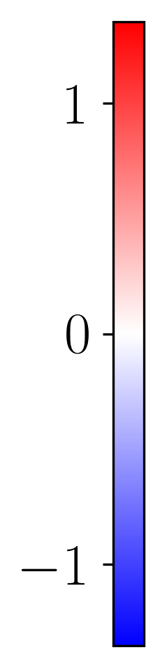
(a) $u_{0}$

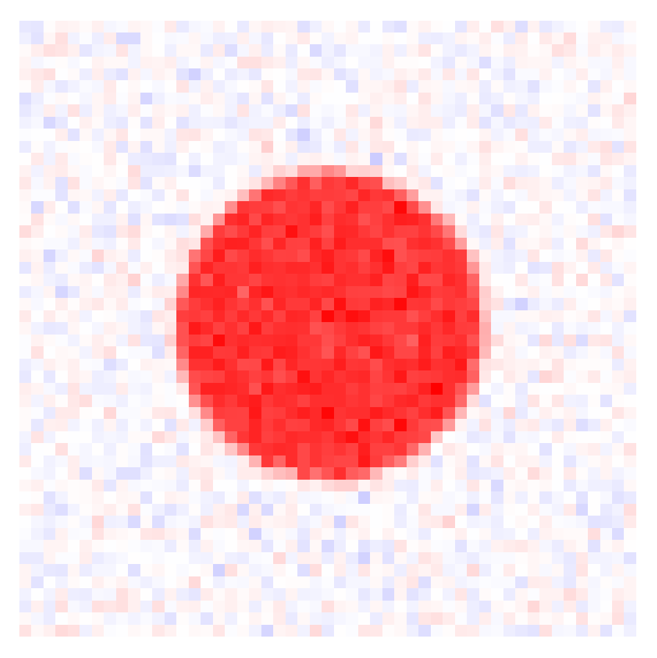
(b) $y_{0}+w$

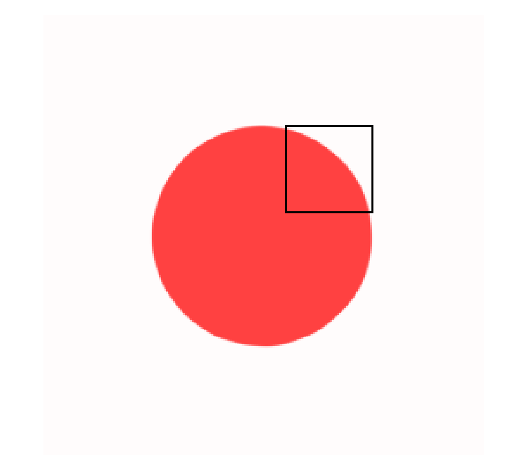
(c) approx. of $u_{\lambda,w}$

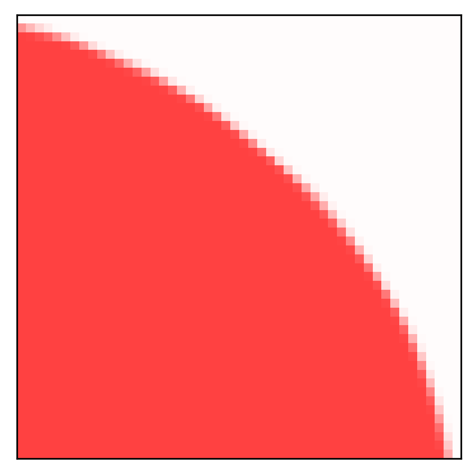
(d)

Figure 1: Numerical resolution of ($\mathcal{P}_{\lambda}(y_{0}+w)$) for $u_{0}=\mathbf{1}_{B(0,R)}$.

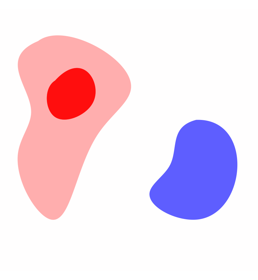
(a) $u_{0}$

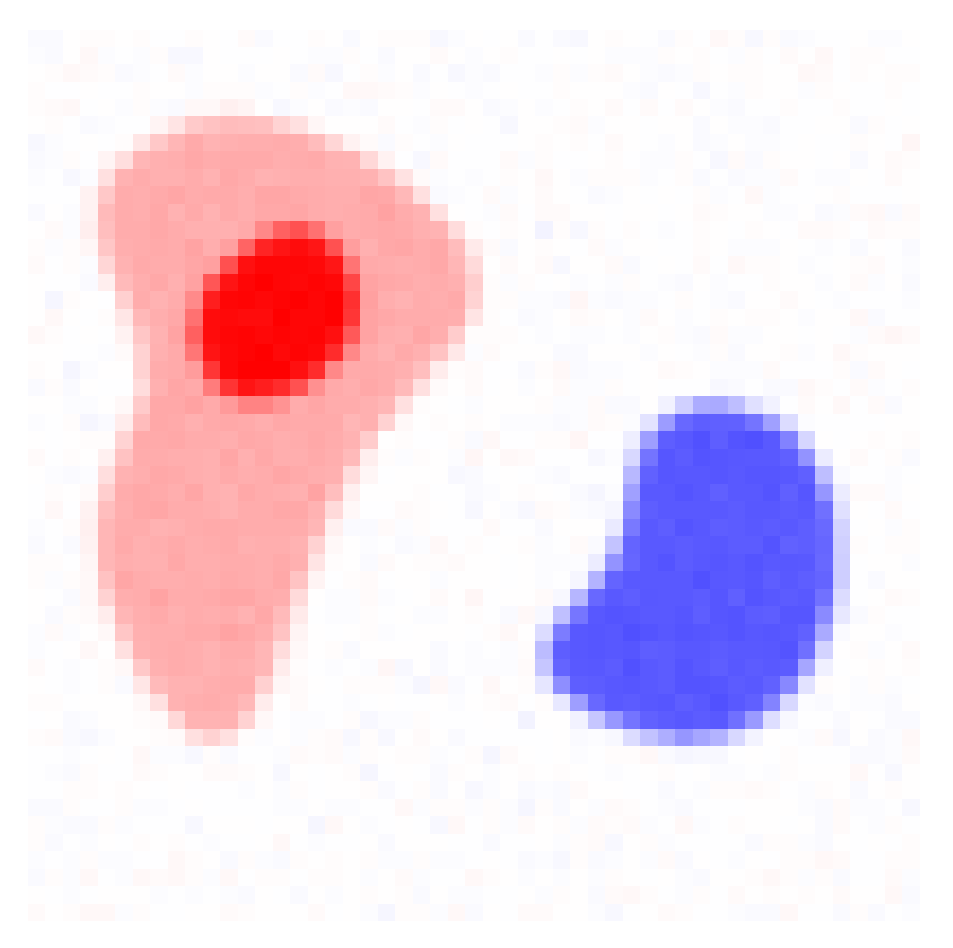
(b) $y_{0}+w$

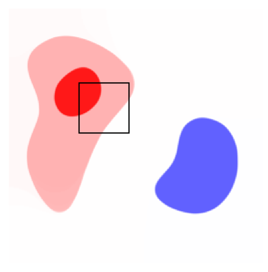
(c) approx. of $u_{\lambda,w}$

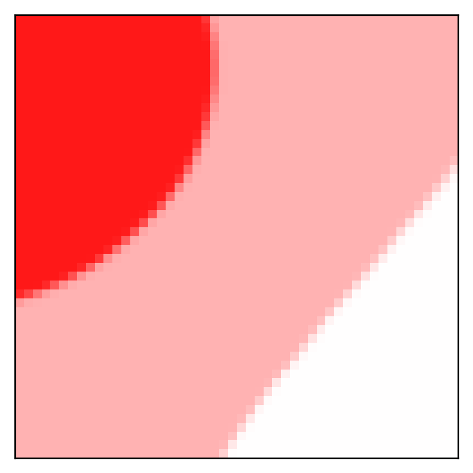
(d)

Figure 2: Numerical resolution of ($\mathcal{P}_{\lambda}(y_{0}+w)$) for $u_{0}=\mathbf{1}_{E_{1}}+2\mathbf{1}_{E_{2}}-2\mathbf{1}_{E_{3}}$.

1.4 Previous works

Total variation minimization in imaging.

The theoretical study of total variation regularization in imaging was initiated in [Chambolle and Lions, 1997, Ring, 2000]. Then, a lot of attention was focused on the denoising case, which can be regarded as one step of the total variation gradient flow, see [Bellettini et al., 2002, Alter et al., 2005b]. Its connection to the Cheeger problem was observed in [Alter et al., 2005a, Alter and Caselles, 2009] and was the key to understanding the properties of the Cheeger sets of convex bodies. Let us also mention the landmark result [Caselles et al., 2007], which shows that the jump set of the reconstructions is included in the jump set of the noisy input. Independently, Allard gave a precise description of the properties of the minimizers in the series of articles [Allard, 2008a, Allard, 2008b, Allard, 2009]. We refer to [Chambolle et al., 2010] for an introduction to total variation references and a much more comprehensive list of bibliographical references.

Piecewise constant images.

Let us emphasize that the above-mentioned representation principle [Boyer et al., 2019, Bredies and Carioni, 2019] only applies to inverse problems with a finite number of measurements. It does not cover the case of denoising or related tasks involving infinite-dimensional observations. For such cases, several authors have proposed specific approaches to promote piecewise constant solutions [Fornasier, 2006, Fornasier and March, 2007, Fonseca et al., 2010, Cristoferi and Fonseca, 2019]. These methods rely on the minimization of non-convex functionals which resemble the $\ell^{0}$ norm, while the total variation relates to the $\ell^{1}$ norm.

Noise robustness.

The general convergence results presented in [Burger and Osher, 2004, Hofmann et al., 2007] apply to the case of total variation regularization, and loosely speaking provide (under mild assumptions) strict convergence in $\mathrm{BV}_{\mathrm{loc}}$ of solutions of ($\mathcal{P}_{\lambda}(y_{0}+w)$) towards solutions of $\mathcal{P}_{0}(y_{0})$. Moreover, in specific cases, the analysis in [Burger and Osher, 2004] ensures that the variation of solutions to ($\mathcal{P}_{\lambda}(y_{0}+w)$) is mostly concentrated in a neighborhood of the support of $\mathrm{D}u_{0}$. In [Chambolle et al., 2016, Iglesias et al., 2018], improved convergence guarantees are derived by exploiting the optimality of level sets of solutions of ($\mathcal{P}_{\lambda}(y_{0}+w)$) for the prescribed curvature problem. The main finding of these works is that, under a few assumptions, the boundaries of the level sets converge in the Hausdorff sense.

Sparse spikes recovery.

Several works have investigated related questions for the sparse spikes recovery problem [De Castro and Gamboa, 2012, Bredies and Pikkarainen, 2013], which consists in recovering a discrete measure from noisy linear measurements. Contrary to our setting, sufficient identifiability conditions have been extensively studied (see for example the landmark paper [Candès and Fernandez-Granda, 2014] or its generalization [Poon et al., 2023]). A series of works has also focused on noise robustness. Among these, let us mention [Duval and Peyré, 2015, Poon and Peyré, 2019], in which structure-preserving convergence results are derived.

1.5 Contributions

In the above-mentioned works, little information about the structure of solutions of (${\mathcal{P}_{\lambda}(y_{0}+w)}$) in the low noise regime is provided. However, in light of the numerical evidence presented in Section 1.3, the following question is natural: if $u_{0}$ is identifiable and is the sum of a few indicator functions, do the solutions of ($\mathcal{P}_{\lambda}(y_{0}+w)$) have a similar property? Moreover, are these decompositions stable, i.e. are they made of the same number of atoms, and are their atoms related?

In this work, we answer these questions by using two main tools. The first is a set of results about the faces of the unit ball defined by the total variation, which provide useful information on the above-mentioned decompositions. The second is an analysis of the behaviour of solutions to the prescribed curvature problem under variations of the curvature functional. To state our main result, we introduce a non-degenerate version of the source condition, which relies on a regularity assumption on the measurement operator $\Phi$, namely that $\phi\in\mathrm{C}^{1}(\mathbb{R}^{2},\mathcal{H})$. This is for instance satisfied if $\Phi$ is the convolution with any $\mathrm{C}^{1}$ filter, possibly followed by a subsampling. However, our assumptions do not cover the case of denoising, which corresponds to $\mathcal{H}=\mathrm{L}^{2}(\mathbb{R}^{2})$ and $\Phi=Id$. In all the following, except in Section 2 in which we review existing results, we assume that $\phi\in\mathrm{C}^{1}(\mathbb{R}^{2},\mathcal{H})$.

Our main result, which is Theorem 5.4, informally states that, if the unknown image modeled by $u_{0}$ is the superposition of a few simple shapes and the non-degenerate source condition holds, then, in the low noise regime, every solution $u_{\lambda,w}$ of ($\mathcal{P}_{\lambda}(y_{0}+w)$) is made of the same number of shapes as $u_{0}$, each shape in $u_{\lambda,w}$ converging smoothly to the corresponding shape in $u_{0}$ as the noise goes to zero (see Figure 3 for an illustration).

(a) $u_{0}$

(b) $u_{\lambda,w}$

Figure 3: Illustration of the result stated in Theorem 5.4. Here $u_{0}$ is equal to $0$ in $A$ and $B$. The values taken by $u_{\lambda,w}$ in $A^{\lambda,w}$ and $B^{\lambda,w}$ are close (but not necessarily equal) to $0$.

2 Preliminaries

2.1 Smooth sets and normal deformations

Our analysis mainly concerns the level sets of the solutions to ($\mathcal{P}_{0}(y_{0})$) and ($\mathcal{P}_{\lambda}(y)$). As we strongly rely on their regularity, we recall here several definitions and properties related to smooth sets and their normal deformations. We refer to [Delfour and Zolesio, 2011] for more details.

Smooth set.

Let $E\subset\mathbb{R}^{2}$ be an open set such that $\partial E\neq\emptyset$, and $k\in\mathbb{N}^{*}$. We say that the set $E$ is of class $\mathrm{C}^{k}$ if, for every $x\in\partial E$, there exists $r_{x}>0$, a rotation matrix $R_{x}$, and a function $u_{x}\in\mathrm{C}^{k}([-r_{x},r_{x}])$ such that

$$\left\{\begin{aligned} R_{x}^{-1}(E-x)\cap C(0,r_{x})&=\left\{(z,t)\in C(0,r_{x})\mid t<u_{x}(z)\right\}\stackrel{{\scriptstyle\mbox{\tiny def.}}}{{=}}\mathrm{hypograph}(u_{x})\,,\\ R_{x}^{-1}(\partial E-x)\cap C(0,r_{x})&=\left\{(z,t)\in C(0,r_{x})\mid t=u_{x}(z)\right\}\stackrel{{\scriptstyle\mbox{\tiny def.}}}{{=}}\mathrm{graph}(u_{x})\,,\end{aligned}\right.$$

where $C(0,r)\stackrel{{\scriptstyle\mbox{\tiny def.}}}{{=}}(-r,r)^{2}$. In that case, one can choose $u_{x}(0)=0$ and $\nabla u_{x}(0)=0$. Moreover, if $\partial E$ is compact, $r_{x}$ can be taken independent of $x$, and the family $\{u_{x}\}_{x\in\partial E}$ uniformly equicontinuous (see [Delfour and Zolesio, 2011, Theorem 5.2]). In local coordinates, the outward unit normal to $E$ at $(z,u_{x}(z))$ is given by

$$\nu_{E}(z,u_{x}(z))=\frac{1}{\sqrt{1+u_{x}^{\prime}(z)^{2}}}\begin{pmatrix}-u_{x}^{\prime}(z)\\ 1\end{pmatrix}\,.$$

It is a geometric quantity, which does not depend on the choice of $r$, $x$ and $u_{x}$. Likewise, the signed curvature of $E$ at $(z,u_{x}(z))$ is given by

$$H_{E}(z,u_{x}(z))=\left(\frac{-u_{x}^{\prime}}{\sqrt{1+u_{x}^{\prime 2}}}\right)^{\prime}(z)=\frac{-u_{x}^{\prime\prime}(z)}{(1+u^{\prime}(z)^{2})^{3/2}}\,.$$

Remark 2.1

The same definitions and properties hold when replacing $\mathrm{C}^{k}$ with $\mathrm{C}^{k,\ell}$ the space of $k$-times continuously differentiable functions whose $k$-th derivative is $\ell$-Hölder ($0<\ell\leq 1$).

Lebesgue equivalence classes and smooth sets.

If $E\subset\mathbb{R}^{2}$ is an open set of class $\mathrm{C}^{1}$ and $x\in\mathbb{R}^{2}$, then its Lebesgue density exists everywhere and it is given by

$$\theta_{E}(x)\stackrel{{\scriptstyle\mbox{\tiny def.}}}{{=}}\underset{r\to 0^{+}}{\mathrm{lim}}~{}\frac{|E\cap B(x,r)|}{|B(x,r)|}=\begin{cases}1&\mbox{if $x\in E$},\\ 1/2&\mbox{if $x\in\partial E$},\\ 0&\mbox{if $x\in\mathbb{R}^{2}\setminus\overline{E}$.}\end{cases}$$ (1)

When working with measurable sets, it is common to regard them modulo Lebesgue negligible sets. The above equality shows that if a measurable set $\tilde{E}\in\mathbb{R}^{2}$ is equivalent to a $\mathrm{C}^{1}$ open set $E$, then $E$ is unique and can be recovered as the set of Lebesgue points of $\tilde{E}$, that is ${\{\theta_{\tilde{E}}=1\}}$. In the following, we usually work with Lebesgue equivalence classes. When $E$ has a $\mathrm{C}^{1}$ open representative, we say that $E$ is of class $\mathrm{C}^{1}$, and we denote by $\partial E$ the topological boundary of that representative.

Convergence.

Let us define the square of axis $\nu\in\mathbb{S}^{1}$ and side $r>0$ centered at $x\in\mathbb{R}^{2}$:

$$C(x,r,\nu)\stackrel{{\scriptstyle\mbox{\tiny def.}}}{{=}}x+R_{\nu}\,C(0,r)\,.$$ (2)

where $R_{\nu}\colon\mathbb{R}^{2}\rightarrow\mathbb{R}^{2}$ is the rotation that maps $(0,1)$ to $\nu$.

Let $E$ be a set of class $\mathrm{C}^{k}$ such that $\partial E$ is compact. We say that a sequence $(E_{n})_{n\in\mathbb{N}}$ converges to $E$ in $\mathrm{C}^{k}$ if there exists ${r>0}$ and $n_{0}\in\mathbb{N}$ such that

• for every $n\geq n_{0}$ we have $\partial E_{n}\subset\bigcup\limits_{x\in\partial E}C(x,r,\nu_{E}(x))$

• for every $n\geq n_{0}$ and $x\in\partial E$ there exists $u_{n,x}\in\mathrm{C}^{k}([-r,r])$ such that:

  $$\left\{\begin{aligned} R_{\nu_{E}(x)}^{-1}\left(\partial E_{n}-x\right)\cap C(0,r)&=\mathrm{graph}(u_{n,x})\\ R_{\nu_{E}(x)}^{-1}\left(\mathrm{int}\,E_{n}-x\right)\cap C(0,r)&=\mathrm{hypograph}(u_{n,x})\end{aligned}\right.$$

• denoting $(u_{x})_{x\in\partial E}$ some functions satisfying

  $$\left\{\begin{aligned} R_{\nu_{E}(x)}^{-1}\left(\partial E-x\right)\cap C(0,r)&=\mathrm{graph}(u_{x})\\ R_{\nu_{E}(x)}^{-1}\left(\mathrm{int}\,E-x\right)\cap C(0,r)&=\mathrm{hypograph}(u_{x})\end{aligned}\right.$$

  we have $\underset{n\to+\infty}{\mathrm{lim}}~{}\underset{x\in\partial E}{\mathrm{sup}}~{}\|u_{n,x}-u_{x}\|_{\mathrm{C}^{k}([-r,r])}=0$

Normal deformation.

We state below some useful results regarding normal deformations of a smooth set $E$. First, let us stress that such sets are parametrized by real-valued functions on $\partial E$, which leads us to use the notion of tangential gradient, tangential Jacobian, and the spaces $\mathrm{C}^{k}(\partial E)$, $\mathrm{L}^{p}(\partial E)$ and $\mathrm{H}^{1}(\partial E)$ (along with their associated norms). We refer to the reader to [Henrot and Pierre, 2018, Section 5.4.1, 5.4.3 and 5.9.1] for precise definitions.

Lemma 2.2

If $E$ is a bounded set of class $\mathrm{C}^{k}$ ($k\geq 2$), then there exists $C>0$ such that, for every $\varphi$ in $\mathrm{C}^{k-1}(\partial E)$, the mapping $\varphi\,\nu_{E}$ can be extended to $\xi_{\varphi}\in\mathrm{C}^{k-1}(\mathbb{R}^{2},\mathbb{R}^{2})$ with

$$\|\xi_{\varphi}\|_{\mathrm{C}^{k-1}(\mathbb{R}^{2},\mathbb{R}^{2})}\leq C\,\|\varphi\|_{\mathrm{C}^{k-1}(\partial E)}\,.$$

Proposition 2.3

Let $E$ be a bounded open set of class $\mathrm{C}^{k}$ (with $k\geq 2$). There exists $c>0$ such that, for every ${\varphi\in\mathrm{C}^{k-1}(\partial E)}$ with $\|\varphi\|_{\mathrm{C}^{k-1}(\partial E)}\leq c$, there is a unique bounded open set of class $\mathrm{C}^{k-1}$, denoted $E_{\varphi}$, satisfying

$$\partial E_{\varphi}=(Id+\varphi\,\nu_{E})(\partial E)\,.$$ (3)

Moreover, there exists an extension $\xi_{\varphi}$ of $\varphi\,\nu_{E}$ such that $E_{\varphi}=(Id+\xi_{\varphi})(E)$ and

$$\|\xi_{\varphi}\|_{\mathrm{C}^{k-1}(\mathbb{R}^{2},\mathbb{R}^{2})}<1\,.$$

In particular, $E_{\varphi}$ is $\mathrm{C}^{k-1}$-diffeomorphic to $E$.

Proposition 2.4

If $(E_{n})_{n\geq 0}$ converges to a bounded set $E$ in $\mathrm{C}^{k}$ with $k\geq 2$, then for $n$ large enough there exists $\varphi_{n}\in\mathrm{C}^{k-1}(\partial E)$ such that $E_{n}=E_{\varphi_{n}}$, and $\|\varphi_{n}\|_{\mathrm{C}^{k-1}(\partial E)}\to 0$.

2.2 Functions of bounded variation and sets of finite perimeter

We recall here a few properties of functions of bounded variation and sets of finite perimeter. More detail can be found in the monogaphs [Ambrosio et al., 2000, Maggi, 2012].

The total variation.

The total variation of a function $u\in\mathrm{L}^{1}_{\mathrm{loc}}(\mathbb{R}^{2})$ is given by

$$\mathrm{TV}(u)\stackrel{{\scriptstyle\mbox{\tiny def.}}}{{=}}\mathrm{sup}\,\bigg{\{}-\int_{\mathbb{R}^{2}}u\,\mathrm{div}\,z\,\bigg{\rvert}\,z\in\mathrm{C}^{\infty}_{c}(\mathbb{R}^{2},\mathbb{R}^{2}),~{}\|z\|_{\infty}\leq 1\bigg{\}}\,.$$

If $\mathrm{TV}(u)$ is finite, then $u$ is said to have bounded variation, and its distributional gradient $\mathrm{D}u$ is a finite Radon measure. In that case, we have $|\mathrm{D}u|(\mathbb{R}^{2})=\mathrm{TV}(u)$. In all the following, we consider $\mathrm{TV}$ as a mapping from $\mathrm{L}^{2}(\mathbb{R}^{2})$ to $\mathbb{R}\cup\{+\infty\}$. This mapping is convex, proper and lower semi-continuous.

Sets of finite perimeter.

If a measurable set $E\subset\mathbb{R}^{2}$ is such that $P(E)\stackrel{{\scriptstyle\mbox{\tiny def.}}}{{=}}\mathrm{TV}(\mathbf{1}_{E})<+\infty$, it is said to be of finite perimeter. If $E$ is an open set of class $\mathrm{C}^{1}$, then $P(E)$ is simply the length of its topological boundary, $P(E)=\mathcal{H}^{1}(\partial E)$, where $\mathcal{H}^{1}$ denotes the one-dimensional Hausdorff measure.

Coarea formula

Functions with bounded variation and sets of finite perimeter are related through the coarea formula [Ambrosio et al., 2000, Thm. 3.40]. For $u\in\mathrm{L}^{1}_{\mathrm{loc}}(\mathbb{R}^{2})$ and ${t\in\mathbb{R}}$, we consider the level sets of $u$,

$$U^{(t)}\stackrel{{\scriptstyle\mbox{\tiny def.}}}{{=}}\begin{cases}\{x\in\mathbb{R}^{2}\,\rvert\,u(x)\geq t\}&\text{if }t\geq 0\,,\\ \{x\in\mathbb{R}^{2}\,\rvert\,u(x)\leq t\}&\text{otherwise.}\end{cases}$$ (4)

It is worth noting that, if $u\in\mathrm{L}^{2}(\mathbb{R}^{2})$, then $|U^{(t)}|<+\infty$ for all $t\neq 0$. The coarea formula states that

$$\forall u\in\mathrm{L}^{2}(\mathbb{R}^{2}),\quad\mathrm{TV}(u) =\int_{-\infty}^{+\infty}P(U^{(t)})\mathrm{d}t.$$ (5)

The isoperimetric inequality.

For every set of finite perimeter $E$, the isoperimetric inequality states that

$$\sqrt{\mathrm{min}(|E|,|E^{c}|)}\leq c_{2}\,P(E)\,,$$ (6)

with equality if and only if $E$ is a ball, and where $c_{2}\stackrel{{\scriptstyle\mbox{\tiny def.}}}{{=}}1/\sqrt{4\pi}$ is the isoperimetric constant (see e.g. [Maggi, 2012, Chapter 14]). In particular, if $E$ is a set of finite perimeter, either $E$ or $E^{c}$ has finite measure. As a consequence of (6) and the coarea formula, the following Poincaré-type inequality holds (see [Ambrosio et al., 2000, Theorem 3.47]),

$$\forall u\in\mathrm{L}^{2}(\mathbb{R}^{2}),\quad\left\|u\right\|_{2}\leq c_{2}\,\mathrm{TV}(u).$$ (7)

Indecomposable and simple sets.

A set of finite perimeter $E\subset\mathbb{R}^{2}$ is said to be decomposable if there exists a partition of $E$ in two sets of positive Lebesgue measure $A$ and $B$ with ${P(E)=P(A)+P(B)}$. We say that $E$ is indecomposable if it is not decomposable. We say that a measurable set $E$ is simple if $E=\mathbb{R}^{2}$, or $|E|<+\infty$ and both $E$ and $\mathbb{R}^{2}\setminus E$ are indecomposable. The importance of simple sets stems from their connection with the extreme points of the total variation unit ball.

Proposition 2.5 ([Fleming, 1957, Ambrosio et al., 2001])

The extreme points of the convex set

$$\{\mathrm{TV}\leq 1\}\stackrel{{\scriptstyle\mbox{\tiny def.}}}{{=}}\left\{u\in\mathrm{L}^{2}(\mathbb{R}^{2})\,\big{\rvert}\,\mathrm{TV}(u)\leq 1\right\}$$

are the functions of the form $\pm\mathbf{1}_{E}/P(E)$, where $E$ is a simple set with $0<|E|<+\infty$.

However, it is worth noting that the exposed points of $\{\mathrm{TV}\leq 1\}$ in the $\mathrm{L}^{2}$ topology (i.e. points that are the only maximizer over $\{\mathrm{TV}\leq 1\}$ of a continuous linear form on $\mathrm{L}^{2}(\mathbb{R}^{2})$) have much more structure (see Sections 3 and 3.3).

2.3 Subdifferential of the total variation

Let us now collect several results on the subdifferential of $\mathrm{TV}$, which are useful to derive and analyze the dual problems of $\mathcal{P}_{0}(y_{0})$ and $\mathcal{P}_{\lambda}(y)$. Since $\mathrm{TV}$ is the support function of the convex set

$$C\stackrel{{\scriptstyle\mbox{\tiny def.}}}{{=}}\left\{\mathrm{div}\,z\,\big{\rvert}\,z\in\mathrm{C}_{c}^{\infty}(\mathbb{R}^{2},\mathbb{R}^{2}),~{}\|z\|_{\infty}\leq 1\right\},$$

its subdifferential at $0$ is the closure of $C$ in $\mathrm{L}^{2}(\mathbb{R}^{2})$, that is

$$\partial\mathrm{TV}(0)=\overline{C}=\left\{\text{div}\,z\,\big{\rvert}\,z\in\mathrm{L}^{\infty}(\mathbb{R}^{2},\mathbb{R}^{2}),~{}\text{div}z\in\mathrm{L}^{2}(\mathbb{R}^{2}),~{}||z||_{\infty}\leq 1\right\}.$$ (8)

We also have the following useful identity:

$$\partial\mathrm{TV}(0)=\left\{\eta\in\mathrm{L}^{2}(\mathbb{R}^{2})\,\bigg{\rvert}\,\forall u\in\mathrm{L}^{2}(\mathbb{R}^{2}),\,\left|\int_{\mathbb{R}^{2}}\eta\,u\right|\leq\mathrm{TV}(u)\right\}.$$ (9)

Finally, the sudifferential of $\mathrm{TV}$ at some $u\in\mathrm{L}^{2}(\mathbb{R}^{2})$ is given by:

$$\partial\mathrm{TV}(u)=\left\{\eta\in\partial\mathrm{TV}(0)\,\bigg{\rvert}\,\int_{\mathbb{R}^{2}}\eta\,u=\mathrm{TV}(u)\right\}\,.$$ (10)

Hence, if $\eta\in\partial\mathrm{TV}(u)$, then $\eta$ is an element of $\partial\mathrm{TV}(0)=\overline{C}$ for which the supremum in the definition of the total variation is attained.

2.4 Dual problems and dual certificates

The backbone of our main result is the relation between the solutions of $\mathcal{P}_{0}(y_{0})$ or $\mathcal{P}_{\lambda}(y)$ and the solutions of their dual problems. We gather here several properties of these dual problems which can be found in [Chambolle et al., 2016] (for the denoising case) and [Iglesias et al., 2018, Section 2] (for the general case).

Dual problems.

The Fenchel-Rockafellar dual problems to $\mathcal{P}_{0}(y_{0})$ and $\mathcal{P}_{\lambda}(y)$ are respectively

$$\underset{p\in\mathcal{H}}{\text{sup}}~{}\langle p,y_{0}\rangle_{\mathcal{H}}~{} \text{ s.t. }\Phi^{*}p\in\partial\mathrm{TV}(0)\,, \mathcal{D}_{0}(y_{0})$$ ()

$$\underset{p\in\mathcal{H}}{\text{sup}}~{}\langle p,y\rangle_{\mathcal{H}}-\frac{\lambda}{2}||p||_{\mathcal{H}}^{2}~{}\text{ s.t. }\Phi^{*}p\in\partial\mathrm{TV}(0)\,. \mathcal{D}_{\lambda}(y)$$ ()

The existence of a solution to $\mathcal{D}_{0}(y_{0})$ does not always hold. On the contrary, $\mathcal{D}_{\lambda}(y)$ can be reformulated as the problem of projecting $y/\lambda$ onto the closed convex set ${\{p\in\mathcal{H}\,\rvert\,\Phi^{*}p\in\partial\mathrm{TV}(0)\}}$, which has a unique solution.

Strong duality.

The values of $\mathcal{P}_{0}(y_{0})$ and $\mathcal{D}_{0}(y_{0})$ are equal. Moreover, if there exists a solution $p$ to $\mathcal{D}_{0}(y_{0})$, then for every solution $u$ of $\mathcal{P}_{0}(y_{0})$ we have

$$\Phi^{*}p\in\partial\mathrm{TV}(u)\,.$$ (11)

Conversely, if $(u,p)\in\mathrm{L}^{2}(\mathbb{R}^{2})\times\mathcal{H}$ with $\Phi u=y_{0}$ and 11 holds, then $u$ and $p$ respectively solve $\mathcal{P}_{0}(y_{0})$ and $\mathcal{D}_{0}(y_{0})$. From the perspective of inverse problems, given some unknown image $u_{0}\in\mathrm{L}^{2}(\mathbb{R}^{2})$ and observation $y_{0}=\Phi u_{0}$, it is therefore sufficient to assume the existence of $p\in\mathcal{H}$ with ${\Phi^{*}p\in\partial\mathrm{TV}(u_{0})}$ to ensure that $u_{0}$ is a solution to $\mathcal{P}_{0}(y_{0})$. This property is known as the source condition [Neubauer, 1989, Burger and Osher, 2004]. If, moreover, $\Phi$ is injective on the cone $\{u\in\mathrm{L}^{2}(\mathbb{R}^{2})\,\rvert\,\Phi^{*}p\in\partial\mathrm{TV}(u)\}$, then $u_{0}$ is the unique solution to  $\mathcal{P}_{0}(y_{0})$.

As in the noiseless case, the values of $\mathcal{P}_{\lambda}(y)$ and $\mathcal{D}_{\lambda}(y)$ are equal. Moreover, denoting by $p$ the unique solution to $\mathcal{D}_{\lambda}(y)$, for every solution $u$ of $\mathcal{P}_{\lambda}(y)$ we have

$$\left\{\begin{aligned} &\Phi u=y-\lambda\,p\,,\\ &\Phi^{*}p\in\partial\mathrm{TV}(u)\,.\end{aligned}\right.$$ (12)

Conversely, if 12 holds, then $u$ and $p$ respectively solve $\mathcal{P}_{\lambda}(y)$ and $\mathcal{D}_{\lambda}(y)$. Although there might not be a unique solution to $\mathcal{P}_{\lambda}(y)$, 12 yields that all of them have the same image by $\Phi$ and the same total variation.

Dual certificates.

If $\eta=\Phi^{*}p$ and $\eta\in\partial\mathrm{TV}(u)$, we call $\eta$ a dual certificate for $u$ with respect to $\mathcal{P}_{0}(y_{0})$, as its existence certifies the optimality of $u$ for $\mathcal{P}_{0}(y_{0})$, provided $y_{0}=\Phi u$. Similarly, if ${\eta=-\Phi^{*}(\Phi u-y)/\lambda}$ and $\eta\in\partial\mathrm{TV}(u)$, we call $\eta$ a dual certificate for $u$ with respect to $\mathcal{P}_{\lambda}(y)$. There could be multiple dual certificates associated to $\mathcal{P}_{0}(y_{0})$. One of them, the minimal norm certificate, plays a crucial role in the analysis of the low noise regime. A quick look at the objective of $\mathcal{D}_{\lambda}(y)$ indeed suggests that, as $\lambda$ goes to $0$, its solution converges to the solution to the limit problem $\mathcal{D}_{0}(y_{0})$ with minimal norm. This is Proposition 2.7 below.

Definition 2.6

If there exists a solution to $\mathcal{D}_{0}(y_{0})$, the minimal norm dual certificate associated to $\mathcal{P}_{0}(y_{0})$, denoted $\eta_{0}$, is defined as

$$\eta_{0}=\Phi^{*}p_{0}~{}\text{ with }~{}p_{0}=\mathrm{argmin}~{}\|p\|_{\mathcal{H}}~{}\text{ s.t. }~{}p\text{ solves }\lx@cref{creftype~refnum}{dual_noreg}\,.$$

If $\lambda>0$, we denote $p_{\lambda,w}$ the unique solution to ($\mathcal{D}_{\lambda}(y_{0}+w)$), and ${\eta_{\lambda,w}=\Phi^{*}p_{\lambda,w}}$ the associated dual certificate. Noise robustness results extensively rely on the behaviour of $\eta_{\lambda,w}$ as $\lambda$ and $w$ go to zero. This behaviour is described by the following results.

Proposition 2.7 ([Chambolle et al., 2016, Prop.6],[Iglesias et al., 2018, Prop. 3])

If there exists a solution to $\mathcal{D}_{0}(y_{0})$, then $p_{\lambda,0}$ converges strongly to $p_{0}$ as ${\lambda\to 0}$.

Since $p_{\lambda,w}$ is the projection of $(y_{0}+w)/\lambda$ onto the closed convex set $\{p\in\mathcal{H}\,\rvert\,\Phi^{*}p\in\partial\mathrm{TV}(0)\}$, the non-expansiveness of the projection mapping yields

$$\forall(\lambda,w)\in\mathbb{R}_{+}^{*}\times\mathcal{H},~{}\|p_{\lambda,w}-p_{\lambda,0}\|_{\mathcal{H}}\leq\frac{\|w\|_{\mathcal{H}}}{\lambda}\,,$$ (13)

and hence

$$\forall(\lambda,w)\in\mathbb{R}_{+}^{*}\times\mathcal{H},~{}\|\eta_{\lambda,w}-\eta_{\lambda,0}\|_{\mathrm{L}^{2}(\mathbb{R}^{2})}\leq\frac{\|\Phi^{*}\|\,\|w\|_{\mathcal{H}}}{\lambda}\,.$$

As a result, if $\lambda\to 0$ and $\|w\|_{\mathcal{H}}/\lambda\to 0$, the dual certificate $\eta_{\lambda,w}$ converges strongly in $\mathrm{L}^{2}(\mathbb{R}^{2})$ to the minimal norm certificate $\eta_{0}$.

2.5 Noise robustness results

Let us now review existing noise robustness results, which we use in various parts of this work. From Proposition 3.1 and the results of Section 2.4, we know that the levels sets of solutions to ($\mathcal{P}_{\lambda}(y_{0}+w)$) are solution to the prescribed curvature problem associated to $\eta_{\lambda,w}$. In [Chambolle et al., 2016, Iglesias et al., 2018], this fact is exploited to obtain uniform properties of the level sets in the low noise regime. We collect the byproducts of this analysis in the following lemma.

Lemma 2.8 ([Chambolle et al., 2016, Section 5])

Let $(\eta_{n})_{n\geq 0}\subset\partial\mathrm{TV}(0)$ be a sequence converging strongly in $\mathrm{L}^{2}(\mathbb{R}^{2})$ to $\eta_{\infty}$, and let $\mathcal{E}$ be defined by

$$\mathcal{E}\stackrel{{\scriptstyle\mbox{\tiny def.}}}{{=}}\left\{E\subset\mathbb{R}^{2},~{}0<|E|<+\infty\,\bigg{\rvert}\,\exists n\in\mathbb{N}\cup\{\infty\},~{}P(E)=\left|\int_{E}\eta_{n}\right|\right\}.$$

Then the following holds:

1. $\underset{E\in\mathcal{E}}{\mathrm{inf}}~{}P(E)>0$ and $\underset{E\in\mathcal{E}}{\mathrm{sup}}~{}P(E)<+\infty$,

2. $\underset{E\in\mathcal{E}}{\mathrm{inf}}~{}|E|>0$ and $\underset{E\in\mathcal{E}}{\mathrm{sup}}~{}|E|<+\infty$,

3. there exists $R>0$ such that, for every $E\in\mathcal{E}$, it holds $E\subset B(0,R)$,

4. there exists $r_{0}>0$ and $C\in(0,1/2)$ such that for every $r\in(0,r_{0}]$ and $E\in\mathcal{E}$:

   $$\forall x\in\partial E,~{}C\leq\frac{|E\cap B(x,r)|}{|B(x,r)|}\leq 1-C\,.$$

In the above-mentioned works, Lemma 2.8 is used to obtain the convergence result of Footnote 1. It indeed allows to show that, in the low noise regime, the solutions to ($\mathcal{P}_{\lambda}(y_{0}+w)$) have bounded support, and therefore belong to $\mathrm{L}^{1}(\mathbb{R}^{2})$. This can in turn be used to show their strict convergence in $\mathrm{BV}(\mathbb{R}^{2})$ towards a solution $u_{*}$ of $\mathcal{P}_{0}(y_{0})$, which in particular imply the weak-* convergence of their gradient (see e.g. [Ambrosio et al., 2000, Proposition 3.13 and Definition 3.14]). Finally, one obtains the convergence of their level set towards those of $u_{*}$ in the Hausdorff sense, which corresponds to the uniform convergence of the associated distance functions (see Theorem 6.1 and its proof in [Ambrosio et al., 2000]).

Proposition 2.9

Assume $\mathcal{D}_{0}(y_{0})$ has a solution, $\lambda_{n}\to 0$ and

$$\frac{\|w_{n}\|_{\mathcal{H}}}{\lambda_{n}}\leq\frac{1}{4c_{2}\,\|\Phi^{*}\|}\,.$$

Then, if $u_{n}$ is a solution of ($\mathcal{P}_{\lambda_{n}}(y_{0}+w_{n})$) for all $n\in\mathbb{N}$, we have that $(\mathrm{Supp}(u_{n}))_{n\geq 0}$ is bounded and that, up to the extraction of a subsequence (not relabeled), $(u_{n})_{n\geq 0}$ converges strictly in $\mathrm{BV}(\mathbb{R}^{2})$ to a solution $u_{*}$ of $\mathcal{P}_{0}(y_{0})$. Moreover, for almost every $t\in\mathbb{R}$, we have:

$$\big{|}U_{n}^{(t)}\triangle U_{*}^{(t)}\big{|}\longrightarrow 0~{}~{}~{}\mathrm{and}~{}~{}~{}\partial U_{n}^{(t)}\longrightarrow\partial U_{*}^{(t)}\,,$$

where the last limit holds in the Hausdorff sense.

3 The exposed faces of the total variation unit ball

We recall that, in the remaining of this work, we assume that $\phi\in\mathrm{C}^{1}(\mathbb{R}^{2},\mathcal{H})$, so that $\Phi^{*}$ is continuous from $\mathcal{H}$ to $\mathrm{C}^{1}(\mathbb{R}^{2})$.

In order to take advantage of the extremality relations (11) and (12), it is important to understand the properties of $u$ implied by the relation $\eta\in\partial\mathrm{TV}(u)$, for a given $\eta\in\partial\mathrm{TV}(0)$. In other words, our goal is to study the set

$$\partial\mathrm{TV}^{*}(\eta)=\left\{u\in\mathrm{L}^{2}(\mathbb{R}^{2})\,\big{\rvert}\,\eta\in\partial\mathrm{TV}(u)\right\}=\underset{u\in\mathrm{L}^{2}(\mathbb{R}^{2})}{\operatorname{Argmax}}\;\left(\int_{\mathbb{R}^{2}}\eta u-\mathrm{TV}(u)\right),$$ (14)

where $\mathrm{TV}^{*}$ denotes the Fenchel conjugate of $\mathrm{TV}$.

3.1 Subgradients and exposed faces

It is possible to relate (14) to the faces of the total variation unit ball, in connection with Fleming’s result (i.e. Proposition 2.5). We say that a set $\mathcal{F}\subseteq\{\mathrm{TV}\leq 1\}$ is an exposed face of ${\{\mathrm{TV}\leq 1\}}$ if there exists $\eta\in\mathrm{L}^{2}(\mathbb{R}^{2})$ such that

$$\mathcal{F}=\underset{u\in\{\mathrm{TV}\leq 1\}}{\operatorname{Argmax}}\;\int_{\mathbb{R}^{2}}\eta u\,.$$ (15)

Exposed faces are closed convex subsets of $\{\mathrm{TV}\leq 1\}$, and they are faces in the classical sense: if $u\in\mathcal{F}$ and $I\subset\{\mathrm{TV}\leq 1\}$ is an open line segment containing $u$, then $I\subset\mathcal{F}$. We refer the reader to [Rockafellar, 1970, Chapter 18] for more detail on faces and exposed faces. To emphasize the dependency on $\eta$ we sometimes write $\mathcal{F}_{\eta}$ for $\mathcal{F}$, and we note that

$$\mathcal{F}_{0}=\{\mathrm{TV}\leq 1\}\quad\mbox{and}\quad\mathcal{F}_{t\eta}=\mathcal{F}_{\eta}\ \mbox{for all $t>0$}.$$

It is also worth considering the corresponding value, which is sometimes called the $G$-norm in the literature [Meyer, 2001, Aujol et al., 2005, Kindermann et al., 2006, Haddad, 2007],

$$\forall\eta\in\mathrm{L}^{2}(\mathbb{R}^{2}),\quad\left\|\eta\right\|_{G}\stackrel{{\scriptstyle\mbox{\tiny def.}}}{{=}}\sup_{u\in\{\mathrm{TV}\leq 1\}}\int_{\mathbb{R}^{2}}\eta u\,.$$

In view of (9), we see that $\eta\in\partial\mathrm{TV}(0)$ if and only if $\left\|\eta\right\|_{G}\leq 1$. Assuming that $\left\|\eta\right\|_{G}\leq 1$, the condition $\int_{\mathbb{R}^{2}}\eta u=\mathrm{TV}(u)$ in (10) is equivalent to $u=0$ or

$$\int_{\mathbb{R}^{2}}\eta\left(\frac{u}{\mathrm{TV}(u)}\right)=1,$$ (16)

the latter equality implying that $\left\|\eta\right\|_{G}=1$ and $u/\mathrm{TV}(u)\in\mathcal{F}_{\eta}$. As a result, we obtain the following description,

$$\mathrm{TV}^{*}(\eta) =\begin{cases}\emptyset&\mbox{if $\left\|\eta\right\|_{G}>1$},\\ \{0\}\cup\left(\bigcup_{t>0}(t\mathcal{F}_{\eta})\right),&\mbox{if $\left\|\eta\right\|_{G}=1$,}\\ \{0\}&\mbox{if $\left\|\eta\right\|_{G}<1$}.\end{cases}$$ (17)

To summarize the connection between subgradients and exposed faces, if $\mathcal{F}$ is a face of $\{\mathrm{TV}\leq 1\}$ exposed by some $\eta\in\mathrm{L}^{2}(\mathbb{R}^{2})\setminus\{0\}$, its conic hull $\mathbb{R}_{+}\mathcal{F}$ is equal to $\partial\mathrm{TV}^{*}(\eta/\left\|\eta\right\|_{G})$. Conversely, if $\left\|\eta\right\|_{G}=1$, then $\partial\mathrm{TV}^{*}(\eta)\cap\{\mathrm{TV}=1\}$ is $\mathcal{F}_{\eta}$, the face of $\{\mathrm{TV}\leq 1\}$ exposed by $\eta$.

In the rest of this section, we fix some $\eta\in\mathrm{L}^{2}(\mathbb{R}^{2})$ such that $\left\|\eta\right\|_{G}=1$ (the only interesting case), and we study $\mathrm{TV}^{*}(\eta)$. Equivalently, we describe all the faces of $\{\mathrm{TV}\leq 1\}$ exposed by nonzero vectors.

3.2 Exposed versus non-exposed faces

The extreme points of $\{\mathrm{TV}\leq 1\}$ are described by Proposition 2.5: those are the (signed, renormalized) indicators of simple sets. The $k$-dimensional faces ($k\in\mathbb{N}$) are more complex, and they involve functions which are piecewise constant on some partition of $\mathbb{R}^{2}$ (see for instance [Duval, 2022], or the monographs [Fujishige, 2005, Bach, 2013] in a finite-dimensional setting). Even though it is known that the $k$-dimensional faces have a finite number of extreme points and are thus polytopes (see [Duval, 2022, Theorem 2.1]), the corresponding partition can be singular and counter-intuitive [Boyer et al., 2023].

However, the faces involved in (17) are the exposed faces, and we emphasize in this section that they have a simpler structure than arbitray faces, especially if $\eta\in\mathrm{C}^{1}$, as is the case in the extremality conditions (11) and (12). We prove in Theorem 3.7 that, under this assumption, the $k$-dimensional exposed faces of $\{\mathrm{TV}\leq 1\}$ are $k$-simplices.

At the core of our discussion is the reformulation of the subdifferential property into a geometric variational problem using level sets and the coarea formula (see (4) and (5)).

Proposition 3.1 ([Kindermann et al., 2006, Chambolle et al., 2016])

Let $u\in\mathrm{L}^{2}(\mathbb{R}^{2})$ be such that ${\mathrm{TV}(u)<+\infty}$, and let ${\eta\in\mathrm{L}^{2}(\mathbb{R}^{2})}$. Then the following conditions are equivalent.

1. $\eta\in\partial\mathrm{TV}(u)\,.$

2. $\eta\in\partial\mathrm{TV}(0)$ and the level sets of $u$ satisfy

   $$\forall t>0,~{}P(U^{(t)})=\int_{U^{(t)}}\eta~{}~{}~{}\text{and }~{}~{}\forall t<0,~{}P(U^{(t)})=-\int_{U^{(t)}}\eta\,.$$

3. The level sets of $u$ satisfy

   $$\forall t>0,~{}U^{(t)}\in\underset{E\subset\mathbb{R}^{2},\,|E|<+\infty}{\mathrm{Argmin}}\left(P(E)-\int_{E}\eta\right),$$

   $$\forall t<0,~{}U^{(t)}\in\underset{E\subset\mathbb{R}^{2},\,|E|<+\infty}{\mathrm{Argmin}}\left(P(E)+\int_{E}\eta\right).$$

3.3 The prescribed curvature problem

The geometric variational problem appearing in Proposition 3.1,

$$\underset{E\subset\mathbb{R}^{2},\,|E|<+\infty}{\mathrm{inf}}~{}J(E)\stackrel{{\scriptstyle\mbox{\tiny def.}}}{{=}}P(E)-\int_{E}\eta\,, \mathcal{PC}(\eta)$$ ()

is called the prescribed curvature problem associated to $\eta$. This terminology stems from the fact that, if $\eta$ is sufficiently regular, every solution to $\mathcal{PC}(\eta)$ has a (scalar) distributional curvature (see [Maggi, 2012, Section 17.3] for a definition) equal to $\eta$. This problem plays a crucial role in the analysis of total variation regularization, as explained below. For now, let us gather some properties of that problem.

Existence of minimizers.

Solutions to $\mathcal{PC}(\eta)$ exist provided $\eta\in\partial\mathrm{TV}(0)$. Indeed, the objective $J$ is nonnegative, and equal to zero for $E=\emptyset$. From Proposition 3.1, we also know there is a non-empty solution as soon as ${\eta\in\partial\mathrm{TV}(u)}$ for some $u\in\mathrm{L}^{2}(\mathbb{R}^{2})\setminus\{0\}$.

Boundedness.

By [Chambolle et al., 2016, Lemma 4], all solutions of $\mathcal{PC}(\eta)$ are included in some common ball, i.e. there exists $R>0$ such that, for every solution $E$ of $\mathcal{PC}(\eta)$, we have ${E\subset B(0,R)}$.

Regularity of the solutions.

The regularity of the solutions to $\mathcal{PC}(\eta)$ is well understood. If $\eta$ is only assumed to be square integrable, the solutions can be singular but they have some weak form of regularity, as shown in [Gonzales et al., 1993]. In particular, it is known that the square $C=[0,1]^{2}$ is not a solution to $\mathcal{PC}(\eta)$ for any $\eta\in\mathrm{L}^{2}(\mathbb{R}^{2})$ (see, e.g. [Meyer, 2001]). As a result, the function $\mathds{1}_{C}/P(C)$ is an extreme point of $\{\mathrm{TV}\leq 1\}$ which is not exposed. More regularity can be obtained by strengthening the integrability and smoothness of $\eta$. If, in addition to being square integrable, ${\eta\in\mathrm{L}^{\infty}_{\mathrm{loc}}(\mathbb{R}^{2})}$ (which ensures that ${\eta\in\mathrm{L}^{\infty}(B(0,R))}$), then any solution to ($\mathcal{PC}(\eta)$) is a strong quasi-minimizer of the perimeter, and, consequently, is equivalent to an open set of class $\mathrm{C}^{1,1}$ (see e.g. [Ambrosio, 2010, Definition 4.7.3 and Theorem 4.7.4]). Furthermore, if $\eta$ is continuous, then the boundary of any solution is locally the graph of a function $u$ which solves (in the sense of distributions) the Euler-Lagrange equation associated to ($\mathcal{PC}(\eta)$), that is (up to a translation and a rotation):

$$\left(\frac{u^{\prime}}{\sqrt{1+{u^{\prime}}^{2}}}\right)^{\prime}\-(z)=\eta(z,u(z))\,.$$ (18)

This in turn implies that $u$ is $\mathrm{C}^{2}$ ($\mathrm{C}^{k+2,\alpha}$ if $\eta\in\mathrm{C}^{k,\alpha}(\mathbb{R}^{2})$) and solves 18 in the classical sense.

3.4 Indicator functions corresponding to a given face

We fix $\eta\in\mathrm{L}^{2}(\mathbb{R}^{2})$ such that $\left\|\eta\right\|_{G}=1$ (hence $\eta\in\partial\mathrm{TV}(0)$), and we study the face $\mathcal{F}$ of $\{\mathrm{TV}\leq 1\}$ exposed by $\eta$. We assume in addition that $\eta\in\mathrm{C}^{1}(\mathbb{R}^{2})$.

As we know that the extreme points of $\mathcal{F}$ must be (signed, renormalized) indicators of simple sets, it is natural to focus on such functions. The main result we prove in this section is the following. propositionextrpointsdisjsupp For any extreme point $u$ of $\mathcal{F}$, there exists a unique pair $(s,E)$, where $E$ is a simply connected open set of class $\mathrm{C}^{3}$ and ${s\in\{-1,1\}}$, such that $u=s\mathds{1}_{E}/P(E)$.

If $u_{1}$ and $u_{2}$ are two distinct extreme points of $\mathcal{F}$, and $\{(s_{i},E_{i})\}_{i=1,2}$ are their corresponding decompositions, then $\partial E_{1}\cap\partial E_{2}=\emptyset$.

To obtain this result, we study the elements of $\mathcal{F}$ which are (proportional to) indicator functions, and we introduce the collection

$$\mathcal{E} \stackrel{{\scriptstyle\mbox{\tiny def.}}}{{=}}\mathcal{E}^{+}\cup\mathcal{E}^{-}\cup\{\emptyset,\mathbb{R}^{2}\}\,,~{}\mbox{where}$$ (19)

$$\mathcal{E}^{+} \stackrel{{\scriptstyle\mbox{\tiny def.}}}{{=}}\left\{E\subset\mathbb{R}^{2}\,\bigg{\rvert}\,|E|<+\infty,~{}0<P(E)<+\infty,~{}\frac{\mathbf{1}_{E}}{P(E)}\in\mathcal{F}\right\},$$

$$\mathcal{E}^{-} \stackrel{{\scriptstyle\mbox{\tiny def.}}}{{=}}\left\{E\subset\mathbb{R}^{2}\,\bigg{\rvert}\,|E^{c}|<+\infty,~{}0<P(E^{c})<+\infty,~{}\frac{-\mathbf{1}_{E^{c}}}{P(E^{c})}\in\mathcal{F}\right\}.$$

If $\left\lvert E\right\rvert<+\infty$ (resp. $\left\lvert E\right\rvert=+\infty$), Proposition 3.1 above shows that $E\in\mathcal{E}^{+}$ (resp. $E\in\mathcal{E}^{-}$) if and only if $E$ is a solution to ($\mathcal{PC}(\eta)$) (resp. $E^{c}$ is a solution to $\mathcal{PC}(-\eta)$).

3.4.1 Structure of $\mathcal{E}$

The collection $\mathcal{E}$ has the remarkable property of being closed under union and intersection.

Proposition 3.2

Let $E\in\mathcal{E}$ and $F\in\mathcal{E}$. Then $E\cap F\in\mathcal{E}$ and $E\cup F\in\mathcal{E}$.

In fact, $\mathcal{E}$ is even closed under countable union and intersection, but we do not need this property here.

Proof.

If $E\in\mathcal{E}^{+}$ and $F\in\mathcal{E}^{+}$ the submodularity of the perimeter (see e.g. [Ambrosio et al., 2001, Proposition 1]) yields:

$$P(E\cap F)+P(E\cup F)\leq P(E)+P(F)=\int_{E}\eta+\int_{F}\eta=\int_{E\cap F}\eta+\int_{E\cup F}\eta\,.$$

We hence obtain:

$$\left(P(E\cap F)-\int_{E\cap F}\eta\right)+\left(P(E\cup F)-\int_{E\cup F}\eta\right)\leq 0\,.$$

By (9), the above two terms are nonnegative, which yields ${E\cap F\in\mathcal{E}^{+}}$ (unless ${E\cap F=\emptyset}$) and $E\cup F\in\mathcal{E}^{+}$. The same argument applies to the complements, when both $E$ and $F$ are in $\mathcal{E}^{-}$. Now, if $E\in\mathcal{E}^{+}$ and $F\in\mathcal{E^{-}}$,

$$P(E\cap F)+P((E\cup F)^{c}) =P(E\cap F)+P(E\cup F)$$

$$\leq P(E)+P(F)$$

$$=P(E)+P(F^{c})$$

$$=\int_{E}\eta-\int_{F^{c}}\eta$$

$$=\int_{E\cap F}\eta-\int_{(E\cup F)^{c}}\eta$$

Reasoning as above, we obtain that $E\cap F\in\mathcal{E}^{+}$ (unless $E\cap F=\emptyset$) and $E\cup F\in\mathcal{E}^{-}$ (unless ${E\cup F=\mathbb{R}^{2}}$). ∎

3.4.2 Relative position of elements of $\mathcal{E}$

In view of the regularity results of Section 3.3 and the assumption that $\eta\in\mathrm{C}^{1}$, the solutions of the prescribed curvature problem associated to $\pm\eta$ (and hence the elements of $\mathcal{E}$) are equivalent to open sets of class $\mathrm{C}^{3}$. This property, together with Proposition 3.2, imposes strong constraints on the intersection of the boundaries of elements of $\mathcal{E}$, as the next proposition shows.

Proposition 3.3

Let $E,F\in\mathcal{E}$. Then

$$\partial E\cap\partial F=\{\nu_{E}=\nu_{F}\}\cup\{\nu_{E}=-\nu_{F}\}\,.$$ (20)

Moreover, the sets $\{\nu_{E}=-\nu_{F}\}$ and $\{\nu_{E}=\nu_{F}\}$ are both open and closed in $\partial E$ and $\partial F$.

Let us recall that the topological boundaries and the normals mentioned above are those of the unique open representative of $E$ (resp. $F$), see Section 2.1. The proof of Proposition 3.3 follows from the next two Lemmas.

Lemma 3.4

Let $E$ and $F$ be two sets of class $\mathrm{C}^{1}$. If $E\cap F$ and $E\cup F$ (modulo a Lebesgue-negligible set) are trivial or $\mathrm{C}^{1}$, then

$$\partial E\cap\partial F=\{\nu_{E}=\nu_{F}\}\cup\{\nu_{E}=-\nu_{F}\}\,$$

and ${\{\nu_{E}=-\nu_{F}\}}$ is both open and closed in $\partial E$ and $\partial F$

Proof.

The regularity of $E,~{}F,~{}E\cap F$ and $E\cup F$ implies that the densities $\theta_{E},~{}\theta_{F},~{}\theta_{E\cap F}$ and $\theta_{E\cup F}$ (defined in Section 2.1) are well-defined on $\mathbb{R}^{2}$ and take values in $\{0,1/2,1\}$. Moreover, since

$$|E\cap B(x,r)|+|F\cap B(x,r)|=|(E\cap F)\cap B(x,r)|+|(E\cup F)\cap B(x,r)|\,,$$

we have:

$$\theta_{E}+\theta_{F}=\theta_{E\cap F}+\theta_{E\cup F}\,.$$

Since $E$ and $F$ are $\mathrm{C}^{1}$, for every $x\in\partial E\cap\partial F$ we have $\theta_{E}(x)=\theta_{F}(x)=1/2$, which yields

$$\theta_{E\cap F}(x)+\theta_{E\cup F}(x)=1\,.$$

Since $\theta_{E\cap F}\leq\theta_{E\cup F}$, we obtain $(\theta_{E\cap F}(x),\theta_{E\cup F}(x))=(0,1)$ or $(\theta_{E\cap F}(x),\theta_{E\cup F}(x))=(1/2,1/2)$.

Now, by a blow-up argument as in the proof of [Maggi, 2012, Theorem 16.3], we note that:

$$\frac{(E\cap F)-x}{r}\cap B(0,1)=\left[\frac{E-x}{r}\cap B(0,1)\right]\cap\left[\frac{F-x}{r}\cap B(0,1)\right]\xrightarrow{r\to 0^{+}}B_{\nu_{E}(x)}^{-}\cap B_{\nu_{F}(x)}^{-}\,,$$

with $B_{\nu}^{-}\stackrel{{\scriptstyle\mbox{\tiny def.}}}{{=}}\left\{x\in B(0,1)\mid\langle x,\nu\rangle\leq 0\right\}$, and where the convergence is in measure. Since, for any measurable set $A$,

$$\left|\frac{A-x}{r}\cap B(0,1)\right|=\frac{|A\cap B(x,r)|}{r^{d}}\,,$$

we deduce that, if $\theta_{E\cap F}(x)=0$, then $|B^{-}_{\nu_{E}(x)}\cap B^{-}_{\nu_{F}(x)}|=0$, hence $\nu_{E}(x)=-\nu_{F}(x)$. Similarly, if $\theta_{E\cap F}(x)=1/2$, then $|B^{-}_{\nu_{E}(x)}\cap B^{-}_{\nu_{F}(x)}|=\pi/2$ and $\nu_{E}(x)=\nu_{F}(x)$.

Let us now prove that $\{\nu_{E}=-\nu_{F}\}$ is both open and closed in $\partial E$ (similar arguments hold for $\partial F$). Since $\nu_{E}$ and $\nu_{F}$ are continuous, the set $\{\nu_{E}=-\nu_{F}\}$ is closed. Now, we show that $\{\nu_{E}=-\nu_{F}\}$ is open in $\partial E$. Let $x\in\partial E$. Since both $E$ and $F$ are of class $\mathrm{C}^{1}$, the above blow-up argument shows that

$$x\in\{\nu_{E}=-\nu_{F}\}\Longleftrightarrow\theta_{E\cap F}(x)=0\ \mbox{and}\ \theta_{E\cup F}(x)=1.$$

Since $E\cap F$ is (equivalent to) the empty set or an open set of class $\mathrm{C}^{1}$, the set $\{\theta_{E\cap F}=0\}$ is open. Similarly, since $E\cup F$ is (equivalent to) $\mathbb{R}^{2}$ or an open set of class $\mathrm{C}^{1}$, the set $\{\theta_{E\cup F}=1\}$ is open. As a result $\{\nu_{E}=-\nu_{F}\}=(\partial E)\cap\{\theta_{E\cap F}=0\}\cap\{\theta_{E\cup F}=1\}$ is open in $\partial E$. ∎

In the next lemma, we prove that $\{\nu_{E}=\nu_{F}\}$ is both open and closed in $\partial E$ and $\partial F$. Contrary to the results of Lemma 3.4, this does not hold in general if we only assume that $E$ and $F$ are sets of class $\mathrm{C}^{1}$ such that $E\cap F$ and $E\cup F$ are also of class $\mathrm{C}^{1}$, as the example given in Figure 4 shows.

Figure 4: An example of two smooth sets $E$ (blue region) and $F$ (hatched region) such that $E\cap F$ and $E\cup F$ are smooth but $\{\nu_{E}=\nu_{F}\}$ is neither open in $\partial E$ nor in $\partial F$.

Lemma 3.5

If $E,F\in\mathcal{E}$ then $\{\nu_{E}=\nu_{F}\}$ is both open and closed in $\partial E$ and $\partial F$.

Proof.

The set $\{\nu_{E}=\nu_{F}\}$ is closed, by continuity of the normals. Let us prove that it is open in $\partial E$ and $\partial F$. We begin with the case $E,F\in\mathcal{E}^{+}$. Let ${x\in\{\nu_{E}=\nu_{F}\}}$, and let us denote $\nu\stackrel{{\scriptstyle\mbox{\tiny def.}}}{{=}}\nu_{E}(x)=\nu_{F}(x)$. There exists $r>0$ such that, in $C(x,r,\nu)$, $\partial E$ and $\partial F$ coincide with the graphs of two $\mathrm{C}^{3}$ functions which solve the prescribed curvature equation

$$\frac{u^{\prime\prime}(z)}{(1+u^{\prime}(z)^{2})^{3/2}}=H(z,u(z))~{}~{}\mathrm{with}~{}~{}H(z,t)=\eta(x+R_{\nu}(z,t))$$ (21)

on $(-r,r)$, with Cauchy data $u(0)=u^{\prime}(0)=0$. The prescribed curvature equation can be reduced to a first order ODE on $\mathbb{R}\times\mathbb{R}^{2}$ defined by the mapping

$$(t,x)\in\mathbb{R}\times\mathbb{R}^{2}\mapsto\begin{pmatrix}x_{2}\\ H(t,x_{1})(1+x_{2}^{2})^{3/2}\end{pmatrix}$$

Since this mapping is locally Lipschitz continuous with respect to its second variable, the Cauchy-Lipschitz theorem ensures that the two functions mentioned above coincide on $(-r,r)$. In particular, as

$$\nu_{E}\left(x+R_{\nu}(z,u(z))\right)=(u^{\prime}(z),-1)/\sqrt{1+(u^{\prime}(z))^{2}}=\nu_{F}\left(x+R_{\nu}(z,u(z))\right),$$

the outer unit normals coincide in $C(x,r,\nu)$. As a result,

$$\{\nu_{E}=\nu_{F}\}\cap C(x,r,\nu)=\partial E\cap C(x,r,\nu)=\partial F\cap C(x,r,\nu)\,.$$

which shows that $\{\nu_{E}=\nu_{F}\}$ is open in $\partial E$ and $\partial F$.

If $E,F\in\mathcal{E}^{-}$, then $E^{c}$ and $F^{c}$ are solutions to $\mathcal{PC}(-\eta)$, hence we may apply the above argument to $E^{c}$ and $F^{c}$, with obvious adaptations, to deduce that $\{\nu_{E^{c}}=\nu_{F^{c}}\}=\{\nu_{E}=\nu_{F}\}$ is open in $\partial E$ and $\partial F$.

If $E\in\mathcal{E}^{+}$ and $F\in\mathcal{E}^{-}$, let $\nu\stackrel{{\scriptstyle\mbox{\tiny def.}}}{{=}}\nu_{E}(x)=\nu_{F}(x)=-\nu_{F^{c}}(x)$. As above, for $r>0$ small enough, $\partial E$ coincides in $C(x,r,\nu)$ with the graph of some function $u$ which satisfies (21), with ${u(0)=0}$, $u^{\prime}(0)=0$. On the other hand, $F^{c}$ is a solution to $\mathcal{PC}(-\eta)$, so that for $r>0$ small enough, it coincides in $C(x,r,-\nu)$ with the solution to

$$\frac{v^{\prime\prime}(z)}{(1+v^{\prime}(z)^{2})^{3/2}}=G(z,v(z))~{}~{}\mathrm{with}~{}~{}G(z,t)=-\eta(x+R_{-\nu}(z,t)),$$ (22)

with $v(0)=0$, $v^{\prime}(0)=0$. Since $C(x,r,-\nu)=C(x,r,\nu)$ and $R_{-\nu}(z,t)=R_{\nu}(z,-t)$ for all ${t\in(-r,r)}$, we observe that $\partial F$ coincides in $C(x,r,\nu)$ with the graph of some function ${\tilde{u}=-v}$ which satisfies (21) with $\tilde{u}(0)=0$, $\tilde{u}^{\prime}(0)=0$. We conclude as before that $u$ and $\tilde{u}$ coincide in $(-r,r)$, so that the set $\{\nu_{E}=\nu_{F}\}$ is open in $\partial E$ and $\partial F$. ∎

Now, we conclude this section by proving Section 3.4, whose statement is recalled below. *

Proof.

If $u$ is an extreme point of $\mathcal{F}$, it must be an extreme point of $\{\mathrm{TV}\leq 1\}$, hence Fleming’s result (Proposition 2.5) implies that ${u=s\mathds{1}_{E}/P(E)}$ for some simple set $E\subset\mathbb{R}^{2}$ with ${0<\left\lvert E\right\rvert<+\infty}$. Now, by Proposition 3.1, $E$ is a solution to $\mathcal{PC}\left(s\eta\right)$, so that $E$ is (equivalent to) an open set of class $\mathrm{C}^{3}$. Since $E$ is simple, that open set is the interior of a rectifiable Jordan curve, as a consequence of [Ambrosio et al., 2001, Theorem 7]. Then, the Jordan-Schoenflies theorem implies that $E$ is homeomorphic to a disk, hence simply connected.

Now, let $u_{1}$ and $u_{2}$ be two distinct extreme points. First, we note that $E_{1}\neq E_{2}$. Otherwise, we would have $s_{1}=-s_{2}$, hence $0=\frac{1}{2}s_{1}\mathds{1}_{E_{1}}/P(E_{1})+\frac{1}{2}s_{2}\mathds{1}_{E_{2}}P(E_{2})\in\mathcal{F}$, so that

$$0=\max_{u\in\{\mathrm{TV}\leq 1\}}\int_{\mathbb{R}^{2}}\eta u=\left\|\eta\right\|_{G}=1,$$

a contradiction.

Hence, $E_{1}\neq E_{2}$, and we recall that $E_{i}\in\mathcal{E}^{+}$ if $s_{i}=1$ and $E_{i}^{c}\in\mathcal{E}^{-}$ if $s_{i}=-1$. From Proposition 3.3, we know that, in any case, $\partial E_{1}\cap\partial E_{2}$ is open and closed in $\partial E_{1}$ and $\partial E_{2}$. Since $\partial E_{1}$ and $\partial E_{2}$ are Jordan curves (in particular, they are connected) this implies $\partial E_{1}\cap\partial E_{2}=\emptyset$ or $\partial E_{1}=\partial E_{2}$. Now, if we had $\partial E_{1}=\partial E_{2}$, the Jordan curve theorem would yield $E_{1}=E_{2}$, which is impossible. As a result, we obtain $\partial E_{1}\cap\partial E_{2}=\emptyset$. ∎

3.5 Structure of finite-dimensional exposed faces

As a consequence of Section 3.4, we obtain the following result.

Corollary 3.6

Every family of pairwise distinct extreme points of $\mathcal{F}$ is linearly independent.

Proof.

Let $(u_{i}=s_{i}\mathbf{1}_{E_{i}}/P(E_{i}))_{i\in I}$ be a family of pairwise distinct extreme points of $\mathcal{F}$. If there exists $\lambda\in\mathbb{R}^{I}$ (if $I$ is infinite, we assume that $\lambda$ vanishes except on a finite set) such that ${\sum_{i\in I}\lambda_{i}u_{i}=0}$, then ${\sum_{i\in I}\lambda_{i}\mathrm{D}u_{i}=0}$. Since, for every $i\neq j$, we have

$${\mathrm{Supp}(\mathrm{D}u_{i})\cap\mathrm{Supp}(\mathrm{D}u_{j})=\partial E_{i}\cap\partial E_{j}=\emptyset}\,,$$

we obtain that the measures $(\mathrm{D}u_{i})_{i\in I}$ have disjoint support, which yields $\lambda_{i}=0$ for every ${i\in I}$. ∎

We eventually deduce the main result of this section.

Theorem 3.7

If $\mathrm{dim}(\mathcal{F})=d<+\infty$ then $\mathcal{F}$ has exactly $d+1$ extreme points. It is a $d$-simplex.

Proof.

Let $u_{1},...,u_{m}$ be distinct extreme points of $\mathcal{F}$. From Corollary 3.6, we know that $u_{1},...,u_{m}$ are linearly independent, which is hence also the case of $u_{2}-u_{1},...,u_{m}-u_{1}$. But since this last family is contained in the direction space of $\mathrm{Aff}(\mathcal{F})$, we obtain $m-1\leq\mathrm{dim}(\mathcal{F})=d$.

Conversely, $\mathcal{F}$ has at least $d+1$ extreme points, otherwise, by Carathéodory’s theorem, it would be contained in a $d-1$-dimensional affine space, a contradiction. ∎

Theorem 3.7 is illustrated in Figure 5 and Figure 6. The 2-face depicted in Figure 5 has more than $3$ extreme points, therefore it is not exposed by any $\mathrm{C}^{1}$ function. On the contrary, Figure 6 illustrates a typical 2-face of $\{\mathrm{TV}\leq 1\}$ exposed by some $\mathrm{C}^{1}$ function: it is a triangle (2-simplex).

[scale=0.5]face4_3d

Figure 5: An example of 2-face of the total variation unit ball $\{\mathrm{TV}\leq 1\}$. Such a face has more than 3 extreme points and therefore it is not exposed by any $\mathrm{C}^{1}$ function, by virtue of Theorem 3.7 (notice that $A\cap B$ and $A\cup B$ are not smooth).

[scale=0.5]face3_3d

Figure 6: An example of 2-face of the total variation unit ball $\{\mathrm{TV}\leq 1\}$ that is exposed by some $\mathrm{C}^{1}$ function. Such a face has exactly 3 extreme points.

If $\mathrm{dim}(\mathcal{F})=d<+\infty$, Carathéodory’s theorem implies that every function $u\in\mathcal{F}$ is of the form

$$u=\sum\limits_{i\in I}a_{i}\mathbf{1}_{E_{i}}\,,\quad\mbox{where $1\leq\mathrm{card}\,I\leq d+1$},\ a\in(\mathbb{R}\setminus\{0\})^{I},$$ (23)

and $\{E_{i}\}_{i\in I}$ is a collection of simple sets with positive finite measure that satisfy

$$\mathrm{TV}(u)=\sum\limits_{i\in I}|a_{i}|P(E_{i})\,.$$

As a consequence of Corollary 3.6 and Theorem 3.7, the decomposition (23) is unique (the $E_{i}^{\prime}s$ must form a subcollection of the extreme points of $\mathcal{F}$, and the corresponding $a_{i}$’s are then uniquely determined).

Coming back to our inverse problem, we deduce that, if some dual certificate $\eta=\Phi^{*}p$, with $p$ a solution to $\mathcal{D}_{0}(y_{0})$, exposes some face $\mathcal{F}$ of $\{\mathrm{TV}\leq\min\eqref{primal_noreg}\}$ with dimension $d$, every solution to ($\mathcal{P}_{0}(y_{0})$) has the form (23). If, moreover, the operator

$$\!\begin{aligned} \Phi_{\mathcal{F}}:\mathbb{R}^{d+1}&\to\mathcal{H}\\ a&\mapsto\Phi\Bigg{(}\sum\limits_{i=1}^{d+1}a_{i}\mathbf{1}_{E_{i}}\Bigg{)}\,,\end{aligned}$$

is injective, the solution is unique. We see that, in that case, total (gradient) variation minimization behaves similarly to $\ell^{1}$ (synthesis) minimization [Chen et al., 1998] or total variation (of Radon measures) minimization [Candès and Fernandez-Granda, 2014], in the sense that the only faces $\mathcal{F}$ that are involved are simplices. In the next sections, we show that, under some stability assumption given below, that similarity also holds at low noise: not only $\mathcal{F}$ (the face of the unknown), but all the faces involved in the solutions of ($\mathcal{P}_{\lambda}(y)$) for small $\lambda$ and small $\left\|w\right\|_{\mathcal{H}}$ are simplices, with the same dimension. Hence, with low noise and regularization, the problem ($\mathcal{P}_{\lambda}(y)$) behaves like the Lasso [Tibshirani, 1996] or the Beurling Lasso [Bredies and Pikkarainen, 2013, Azaïs et al., 2015, Duval and Peyré, 2015].

In our context, the equivalent notion to $k$-sparse vectors (or measures) is the following class of piecewise constant functions.

Definition 3.8 ($k$-simple functions)

If $k\in\mathbb{N}^{*}$, we say that a function $u:\mathbb{R}^{2}\to\mathbb{R}$ is $k\text{-simple}$ if there exists a collection $\{E_{i}\}_{1\leq i\leq k}$ of simple sets of class $\mathrm{C}^{1}$ with positive finite measure such that ${\partial E_{i}\cap\partial E_{j}=\emptyset}$ for every $i\neq j$, and $a\in\mathbb{R}^{k}$ such that

$$u=\sum\limits_{i=1}^{k}a_{i}\mathbf{1}_{E_{i}}\,.$$

In particular $1$-simple functions are (proportional to) indicators of simple sets.

The next step is thus to study the stability of $k$-simple functions with respect to noise and regularization: if $u_{0}$ is $k$-simple and identifiable, with $w$ and $\lambda$ small enough, are the solutions of ($\mathcal{P}_{\lambda}(y_{0}+w)$) $k$-simple? What is the number of atoms appearing in their decomposition, and how are they related to those appearing in the decomposition of $u_{0}$?

4 Stability analysis of the prescribed curvature problem

The simple sets appearing in the decomposition of any solution to ($\mathcal{P}_{\lambda}(y_{0}+w)$) are all solutions of the prescribed curvature problem associated to $\eta_{\lambda,w}$. In Section 2.4, we have also seen that, under a few assumptions, $\eta_{\lambda,w}$ converges to the minimal norm certificate $\eta_{0}$ when $w$ and $\lambda$ go to zero. It is therefore natural to investigate how solutions of the prescribed curvature problem behave under variations of the curvature functional.

In this section, we consider the prescribed curvature problem $\mathcal{PC}(\eta)$ associated to some function ${\eta\in\partial\mathrm{TV}(0)\cap\mathrm{C}^{1}(\mathbb{R}^{2})}$. We investigate how the solution set of $\mathcal{PC}(\eta)$ behaves when $\eta$ varies. To be more specific, given two sufficiently close curvature functionals $\eta$ and $\eta^{\prime}$, we address the following two questions.

1. Are the solutions to ($\mathcal{PC}(\eta^{\prime})$) close to some solutions to ($\mathcal{PC}(\eta)$)?

2. How many solutions to ($\mathcal{PC}(\eta^{\prime})$) are there in a neighborhood of a given solution to ($\mathcal{PC}(\eta)$)?

We answer the first question using the notion of quasi-minimizers of the perimeter, as well as first order optimality conditions for $\mathcal{PC}(\eta)$. Then, under a strict stability assumption on solutions to $\mathcal{PC}(\eta)$, we answer the second question using second order shape derivatives.

Convergence result.

First, we tackle Question (i) with the following proposition which states that any neighborhood (in terms of $\mathrm{C}^{2}$-normal deformations) of the solution set of (${\mathcal{PC}(\eta_{0})}$) contains the solution set of $\mathcal{PC}(\eta)$ provided $\eta$ is sufficiently close to $\eta_{0}$ in $\mathrm{C}^{1}(\mathbb{R}^{2})$ and $\mathrm{L}^{2}(\mathbb{R}^{2})$. The proof, which relies on standard compactness results for quasi-minimizers of the perimeter, is postponed to Appendix A.

Proposition 4.1

Let $\eta_{0}\in\partial\mathrm{TV}(0)\cap\mathrm{C}^{1}(\mathbb{R}^{2})$. For every $\epsilon>0$ there exists $r>0$ such that for every ${\eta\in\partial\mathrm{TV}(0)}\cap\mathrm{C}^{1}(\mathbb{R}^{2})$ with ${\|\eta-\eta_{0}\|_{\mathrm{L}^{2}(\mathbb{R}^{2})}+\|\eta-\eta_{0}\|_{\mathrm{C}^{1}(\mathbb{R}^{2})}\leq r}$, the following holds: every non-empty solution $F$ of $\mathcal{PC}(\eta)$ is a $\mathrm{C}^{2}$-normal deformation of size at most $\epsilon$ of a non-empty solution $E$ of ($\mathcal{PC}(\eta_{0})$), i.e., using the notation of Proposition 2.3, $F=E_{\varphi}$ with ${\|\varphi\|_{\mathrm{C}^{2}(\partial E)}\leq\epsilon}$.

4.1 Stability result

Question (ii) is closely linked to the stability of minimizers to $\mathcal{PC}(\eta)$, that is to the behaviour of the objective $J$ in a neighborhood of a solution. To analyze this behaviour, we use the general framework presented in [Dambrine and Lamboley, 2019], which relies on the notion of second order shape derivative. In this section, unless otherwise stated, $E$ denotes a non-empty bounded open set of class $\mathrm{C}^{2}$.

Approach.

The natural path to obtain our main stability result, which is Proposition 4.5, is to prove that $J$ is in some sense of class $\mathrm{C}^{2}$, i.e. that its second order shape derivative is continuous at zero (see Proposition 4.3 for a precise statement). Although it is likely to be known, we could not find this result in the literature. We postpone its proof to Section A.2. To obtain Proposition 4.5, we had to use a stronger condition than the “improved continuity condition” $(\mathbf{IC}_{\mathrm{H}^{1},\mathrm{C}^{2}})$ of [Dambrine and Lamboley, 2019], which is satisfied by our functional. The latter only requires some uniform control of second order directional derivatives at zero, which is weaker than the result of Proposition 4.3.

Structure of shape derivatives.

We introduce the following mapping, where $E_{\varphi}$ denotes the normal deformation of $E$ associated to $\varphi$, defined in Proposition 2.3:

$$\!\begin{aligned} \mathrm{j}_{E}:\mathrm{C}^{1}(\partial E)&\to\mathbb{R}\\ \varphi&\mapsto J(E_{\varphi})\,.\end{aligned}$$

With this notation, the following result holds.

Proposition 4.2 (See e.g. [Henrot and Pierre, 2018, Chapter 5])

If $\eta\in\mathrm{C}^{1}(\mathbb{R}^{2})$, then $\mathrm{j}_{E}$ is twice Fréchet differentiable at $0$ and, for every $\psi\in\mathrm{C}^{1}(\partial E)$, we have:

$$\mathrm{j}^{\prime}_{E}(0).(\psi) =\int_{\partial E}\left[H-\eta\right]\psi\,d\mathcal{H}^{1}$$

$$\mathrm{j}^{\prime\prime}_{E}(0).(\psi,\psi) =\int_{\partial E}\left[|\nabla_{\tau}\psi|^{2}-\left(H\,\eta+\frac{\partial\eta}{\partial\nu}\right)\psi^{2}\right]d\mathcal{H}^{1}$$

where $H$ denotes the curvature of $E$ and $\nabla_{\tau}\psi\stackrel{{\scriptstyle\mbox{\tiny def.}}}{{=}}\nabla\psi-(\nabla\psi\cdot\nu)\,\nu$ is the tangential gradient of $\psi$ with respect to $E$.

From the expression of $\mathrm{j}^{\prime}_{E}(0)$ and $\mathrm{j}^{\prime\prime}_{E}(0)$ given above, we immediately notice that $\mathrm{j}^{\prime}_{E}(0)$ can be extended to a continuous linear form on $\mathrm{L}^{1}(\partial E)$, and $\mathrm{j}^{\prime\prime}_{E}(0)$ to a continuous bilinear form on ${\mathrm{H}^{1}(\partial E)}$.

Strict stability.

Following [Dambrine and Lamboley, 2019], we say that a non-empty open solution $E$ of ($\mathcal{PC}(\eta)$) is strictly stable if $\mathrm{j}^{\prime\prime}_{E}(0)$ is coercive in ${\mathrm{H}^{1}(\partial E)}$, i.e. if the following property holds:

$$\exists\alpha>0,~{}\forall\psi\in\mathrm{H}^{1}(\partial E),\quad\mathrm{j}^{\prime\prime}_{E}(0).(\psi,\psi)\geq\alpha\,\|\psi\|_{\mathrm{H}^{1}(\partial E)}^{2}\,.$$

As noticed by Dambrine and Lamboley, this strict stability condition is a key ingredient (together with several assumptions) to ensure that $E$ is a strict local minimizer of $J$ (see Theorem 1.1 in the above-mentioned reference), and is hence the only minimizer among the sets $E_{\varphi}$ with $\varphi$ in a neighborhood of $0$. It plays a crucial role in our answer to Question (ii).

Continuity results.

Now, we state two important results concerning the convergence of $\mathrm{j}^{\prime\prime}_{E}$ towards $\mathrm{j}^{\prime\prime}_{0,E}$ and the continuity of ${\varphi\mapsto\mathrm{j}^{\prime\prime}_{E}(\varphi)}$, where $\mathrm{j}_{E}$ and $\mathrm{j}_{0,E}$ are the functionals respectively associated to $\eta$ and $\eta_{0}$. Their proof is postponed to Section A.2. In all the following, if $X$ is a (real) vector space, we denote by $\mathcal{Q}(X)$ the set of quadratic forms over $X$, and define $\|\cdot\|_{\mathcal{Q}(X)}$ as follows:

$$\|q\|_{\mathcal{Q}(X)}\stackrel{{\scriptstyle\mbox{\tiny def.}}}{{=}}\underset{x\in X\setminus\{0\}}{\mathrm{sup}}~{}\frac{\left\lvert q(x,x)\right\rvert}{\|x\|_{X}^{2}}$$

Proposition 4.3

If $\eta\in\mathrm{C}^{1}(\mathbb{R}^{2})$, the mapping

$$\!\begin{aligned} \mathrm{j}^{\prime\prime}_{E}:\mathrm{C}^{2}(\partial E)&\to\mathcal{Q}(\mathrm{H}^{1}(\partial E))\\ \varphi&\mapsto\mathrm{j}^{\prime\prime}_{E}(\varphi)\end{aligned}$$

is continuous at $0$.

Proposition 4.4

Let $\eta_{0}\in\mathrm{C}^{1}(\mathbb{R}^{2})$. There exists $\epsilon>0$ such that

$$\underset{\|\eta-\eta_{0}\|_{\mathrm{C}^{1}(\mathbb{R}^{2})}\to 0}{\mathrm{lim}}~{}\underset{\|\varphi\|_{\mathrm{C}^{2}(\partial E)}\leq\epsilon}{\mathrm{sup}}~{}\left\|\mathrm{j}^{\prime\prime}_{E}(\varphi)-\mathrm{j}^{\prime\prime}_{0,E}(\varphi)\right\|_{\mathcal{Q}(\mathrm{H}^{1}(\partial E))}=0\,.$$

Stability result.

We are now able to state the final result of this section, which states that if $E$ is a strictly stable solution to ($\mathcal{PC}(\eta_{0})$), there is at most one $\varphi$ in a neighborhood of $0$ such that $E_{\varphi}$ is a solution to ($\mathcal{PC}(\eta)$), provided $\|\eta-\eta_{0}\|_{\mathrm{C}^{1}(\mathbb{R}^{2})}$ is small engouh.

Proposition 4.5

Let $\eta_{0}\in\partial\mathrm{TV}(0)\cap\mathrm{C}^{1}(\mathbb{R}^{2})$ and $E$ be a strictly stable solution to ($\mathcal{PC}(\eta_{0})$). Then there exists ${\epsilon>0}$ and $r>0$ such that for every $\eta\in\partial\mathrm{TV}(0)$ with $\|\eta-\eta_{0}\|_{\mathrm{C}^{1}(\mathbb{R}^{2})}\leq r$ there is at most one ${\varphi\in\mathrm{C}^{2}(\partial E)}$ such that ${\|\varphi\|_{\mathrm{C}^{2}(\partial E)}\leq\epsilon}$ and $E_{\varphi}$ solves ($\mathcal{PC}(\eta)$).

Proof.

The fact that $E$ is a strictly stable solution to ($\mathcal{PC}(\eta_{0})$) and the results above give the existence of $\epsilon>0$, $r>0$ and $\alpha>0$ such that, for every $(\varphi,\eta)\in\mathrm{C}^{2}(\partial E)\times\mathrm{C}^{1}(\mathbb{R}^{2})$ with $\|\varphi\|_{\mathrm{C}^{2}(\partial E)}\leq\epsilon$ and ${\|\eta-\eta_{0}\|_{\mathrm{C}^{1}(\mathbb{R}^{2})}\leq r}$, we have:

$$\underset{\psi\in\mathrm{H}^{1}(\partial E)\setminus\{0\}}{\mathrm{sup}}~{}\frac{\mathrm{j}^{\prime\prime}_{E}(\varphi).(\psi,\psi)}{\|\psi\|_{\mathrm{H}^{1}(\partial E)}^{2}}\geq\alpha$$

As a result, $\mathrm{j}^{\prime\prime}_{E}(\varphi)$ is coercive (and hence positive definite) for every $\varphi$ such that $\|\varphi\|_{\mathrm{C}^{2}(\partial E)}\leq\epsilon$. We therefore obtain that $\mathrm{j}_{E}$ is strictly convex on this set and the result follows. ∎

Summary.

Combining the results of Propositions 4.1 and 4.5, we have proved that, provided $\eta$ is sufficiently close to $\eta_{0}$ in $\mathrm{C}^{1}(\mathbb{R}^{2})$ and $\mathrm{L}^{2}(\mathbb{R}^{2})$, every solution to $\mathcal{PC}(\eta)$ belongs to a neighborhood (in terms of $\mathrm{C}^{2}$-normal deformations) of a solution to (${\mathcal{PC}(\eta_{0})}$), and that, under a strict stability assumption, each of these neighborhoods contains at most one solution to $\mathcal{PC}(\eta)$. In Section 4.2 below, we discuss this strict stability assumption in greater details. Then, in Theorem 5.4, we prove (under suitable assumptions) that, if $\eta=\eta_{\lambda,w}$ is the dual certificate associated to ($\mathcal{P}_{\lambda}(y_{0}+w)$) and $\eta_{0}$ the minimal norm dual certificate associated to $\mathcal{P}_{0}(y_{0})$, then each neighborhood of a solution to (${\mathcal{PC}(\eta_{0})}$) contains exactly one solution to (${\mathcal{PC}(\eta_{\lambda,w})}$).

4.2 A sufficient condition for strict stability

As mentioned above, we here discuss how to ensure that a non-empty open solution to $\mathcal{PC}(\eta)$ is strictly stable. We derive a sufficient condition for this property to hold, and then discuss to what extent it is necessary.

Setting.

We fix $\eta\in\partial\mathrm{TV}(0)\cap\mathrm{C}^{1}(\mathbb{R}^{2})$ and $E$ a non-empty open solution to $\mathcal{PC}(\eta)$. We recall that, necessarily, $H_{E}=\eta$ on $\partial E$, and the quadratic form $\mathrm{j}^{\prime\prime}_{E}(0)$ is positive semi-definite. By definition, the set $E$ is a strictly stable solution to $\mathcal{PC}(\eta)$ if and only if $\mathrm{j}^{\prime\prime}_{E}(0)$ is coercive in $\mathrm{H}^{1}(\partial E)$, with

$$\forall\psi\in\mathrm{H}^{1}(\partial E),~{}\mathrm{j}^{\prime\prime}_{E}(0).(\psi,\psi)=\int_{\partial E}\left[|\nabla_{\tau_{E}}\psi|^{2}-\left(H_{E}^{2}+\frac{\partial\eta}{\partial\nu_{E}}\right)\psi^{2}\right]d\mathcal{H}^{1}\,.$$

Equivalence of coercivity and positive definiteness.

As explained (in a more general context) in [Dambrine and Lamboley, 2019], the bilinear form $\mathrm{j}^{\prime\prime}_{E}(0)$ is in fact coercive if and only if it is positive definite. Our functional $J$ fits the assumptions of Lemma 3.1 in the above reference. Indeed, writing $\mathrm{j}^{\prime\prime}_{E}(0)=\ell_{m}+\ell_{r}$ with

$$\ell_{m}(\psi,\psi) =\int_{\partial E}|\nabla_{\tau_{E}}\psi|^{2}\,,$$

$$\ell_{r}(\psi,\psi) =-\int_{\partial E}\left[\left(H_{E}^{2}+\frac{\partial\eta}{\partial\nu_{E}}\right)\psi^{2}\right]d\mathcal{H}^{1}\,,$$

we see that $\mathrm{j}^{\prime\prime}_{E}(0)$ satisfies $(\mathbf{C}_{\mathrm{H}^{s_{2}}})$ with $s_{1}=s_{2}=1$. We consequently obtain the following result, which we do not use in the following but which is interesting in itself.

Lemma 4.6 ([Dambrine and Lamboley, 2019, Lemma 3.1])

The following two propositions are equivalent:

1. $\mathrm{j}^{\prime\prime}_{E}(0)$ is positive definite, i.e.

   $$\forall\psi\in\mathrm{H}^{1}(\partial E)\setminus\{0\},\quad\mathrm{j}^{\prime\prime}_{E}(0).(\psi,\psi)>0\,,$$

2. $\mathrm{j}^{\prime\prime}_{E}(0)$ is coercive, i.e.

   $$\exists\alpha>0,~{}\forall\psi\in\mathrm{H}^{1}(\partial E),\quad\mathrm{j}^{\prime\prime}_{E}(0).(\psi,\psi)\geq\alpha\|\psi\|_{\mathrm{H}^{1}(\partial E)}^{2}\,.$$

A sufficient condition for coercivity.

Using the expression of $\mathrm{j}^{\prime\prime}_{E}(0)$, the following result can be directly obtained.

Proposition 4.7

If

$$\underset{x\in\partial E}{\mathrm{sup}}\left[H_{E}(x)^{2}+\frac{\partial\eta}{\partial\nu_{E}}(x)\right]<0\,,$$ (24)

then $\mathrm{j}^{\prime\prime}_{E}(0)$ is coercive.

Necessity of the condition?

A natural question is whether the condition in Proposition 4.7 is necessary. We conjecture that it is not the case. Indeed, assuming that $E$ is simple and $\gamma$ is an arc-length parametrization of $\partial E$, we have:

$$\forall\psi\in\mathrm{H}^{1}(\partial E),~{}\mathrm{j}^{\prime\prime}_{E}(0).(\psi,\psi)=\int_{I}(\psi\circ\gamma)^{\prime 2}-\bigg{(}\bigg{(}H_{E}^{2}+\frac{\partial\eta}{\partial\nu_{E}}\bigg{)}\circ\gamma\bigg{)}\,(\psi\circ\gamma)^{2}\,,$$ (25)

where $I\stackrel{{\scriptstyle\mbox{\tiny def.}}}{{=}}(0,\mathcal{H}^{1}(\partial E))$. The existence of $\psi\neq 0$ such that $\mathrm{j}^{\prime\prime}_{E}(0).(\psi,\psi)=0$ is hence equivalent to the existence of a non-zero minimizer of $\int_{I}\varphi^{\prime 2}+V\varphi^{2}$ under periodicity constraint, where

$${V\stackrel{{\scriptstyle\mbox{\tiny def.}}}{{=}}-\left(H_{E}^{2}+\frac{\partial\eta}{\partial\nu_{E}}\right)\circ\gamma}\,.$$

The first order optimality condition associated to this problem writes ${-\varphi^{\prime\prime}+V\varphi=0}$. The coercivity of $\mathrm{j}^{\prime\prime}_{E}(0)$ can hence be related to the spectrum of the Schrödinger operator with periodic boundary conditions associated to $V$. It is known that there exist potentials $V$ which are not positive and yet correspond to positive definite Schrödinger operators. Therefore, it might be possible to construct examples where (24) does not hold and yet $\mathrm{j}^{\prime\prime}_{E}(0)$ is positive definite.

However, as we explain in Proposition 4.8, if $H_{E}^{2}+\frac{\partial\eta}{\partial\nu_{E}}\geq\alpha$ on a connected portion $\Gamma$ of $\partial E$ and $\alpha\geq(\pi/\mathcal{H}^{1}(\Gamma))^{2}$, we are able to prove that $\mathrm{j}^{\prime\prime}_{E}(0)$ is not coercive. Let us consider a $\mathrm{C}^{1}$ simple open curve $\Gamma$ with finite length. We define the first Dirichlet eigenvalue of the Laplacian associated to $\Gamma$ by:

$$\lambda_{1}(\Gamma)\stackrel{{\scriptstyle\mbox{\tiny def.}}}{{=}}\underset{\psi\in\mathrm{H}_{0}^{1}(\Gamma)\setminus\{0\}}{\mathrm{inf}}~{}\frac{\|\nabla_{\tau_{\Gamma}}\psi\|^{2}_{\mathrm{L}^{2}(\Gamma)}}{\|\psi\|^{2}_{\mathrm{L}^{2}(\Gamma)}}\,.$$ (26)

Using a change of variable as in 25, one can see that the infimum in 26 is attained and is actually equal to the Dirichlet eigenvalue of the interval ${I=(0,\mathcal{H}^{1}(\Gamma))\subset\mathbb{R}}$, which is $(\pi/\mathcal{H}^{1}(\Gamma))^{2}$. Using this fact, we can now prove the following result.

Proposition 4.8

If there exists $\alpha>0$ such that $H_{E}^{2}+\frac{\partial\eta}{\partial\nu_{E}}\geq\alpha$ on a connected subset $\Gamma$ of $\partial E$ with $\alpha\geq(\pi/\mathcal{H}^{1}(\Gamma))^{2}$, then $\mathrm{j}^{\prime\prime}_{E}(0)$ is not coercive.

Proof.

Since the infimum in the definition of $\lambda_{1}(\Gamma)$ is attained, we have the existence of a nonzero function ${\varphi\in\mathrm{H}^{1}_{0}(\Gamma)}$ such that

$$\frac{\|\nabla_{\tau_{\Gamma}}\varphi\|^{2}_{\mathrm{L}^{2}(\Gamma)}}{\|\varphi\|^{2}_{\mathrm{L}^{2}(\Gamma)}}=\lambda_{1}(\Gamma)=\left(\frac{\pi}{\mathcal{H}^{1}(\Gamma)}\right)^{2}\leq\alpha\,.$$

We hence obtain

$$\int_{\Gamma}\left[|\nabla_{\tau_{\Gamma}}\varphi|^{2}-\left(H_{E}^{2}+\frac{\partial\eta}{\partial\nu_{E}}\right)\varphi^{2}\right]d\mathcal{H}^{1}\leq\int_{\Gamma}\left[|\nabla_{\tau_{\Gamma}}\varphi|^{2}-\alpha\,\varphi^{2}\right]d\mathcal{H}^{1}\leq 0\,.$$

We can then extend $\varphi$ to $\psi\in\mathrm{H}^{1}(\partial E)$ whose support is compactly included in $\Gamma$, which yields

$$\int_{\partial E}\left[|\nabla_{\tau_{E}}\psi|^{2}-\left(H_{E}^{2}+\frac{\partial\eta}{\partial\nu_{E}}\right)\psi^{2}\right]d\mathcal{H}^{1}\leq 0\,.$$

We can therefore conclude that $\mathrm{j}^{\prime\prime}_{E}(0)$ is not coercive. ∎

5 Exact support recovery

To obtain our support recovery result, which is Theorem 5.4, we first prove a stability result for the exposed faces of the total variation unit ball, which is Theorem 5.1.

5.1 Stability of the exposed faces of the total variation unit ball

Notations and definitions.

In the following, if $\eta$ (resp. $\eta_{n}$) belongs to $\partial\mathrm{TV}(0)\cap\mathrm{C}^{1}(\mathbb{R}^{2})$, we denote by $\mathcal{F}$ (resp. by $\mathcal{F}_{n}$) the face of $\{\mathrm{TV}\leq 1\}$ exposed by $\eta$. We say that $s\,\mathbf{1}_{E}/P(E)\in\mathrm{extr}(\mathcal{F})$ is strictly stable if $s=1$ and $E$ is a strictly stable solution to ($\mathcal{PC}(\eta)$) or $s=-1$ and $E$ is a strictly stable solution to ($\mathcal{PC}(-\eta)$).

Theorem 5.1

Let $\eta_{0}\in\partial\mathrm{TV}(0)\cap\mathrm{C}^{1}(\mathbb{R}^{2})$ be such that $\mathcal{F}_{0}$ has finite dimension, with all its extreme points strictly stable. Then for every $\epsilon>0$, there exists $r>0$ such that, for every ${\eta\in\partial\mathrm{TV}(0)\cap\mathrm{C}^{1}(\mathbb{R}^{2})}$ with

$$\|\eta-\eta_{0}\|_{\mathrm{L}^{2}(\mathbb{R}^{2})}+\|\eta-\eta_{0}\|_{\mathrm{C}^{1}(\mathbb{R}^{2})}\leq r\,,$$

there exists an injective mapping $\theta:\mathrm{extr}(\mathcal{F})\to\mathrm{extr}({\mathcal{F}_{0}})$ such that, for every ${u=s\,\mathbf{1}_{F}/P(F)}$ in $\mathrm{extr}(\mathcal{F})$, we have $\theta(u)=s\,\mathbf{1}_{E}/P(E)$ with

$$F=E_{\varphi}~{}\mathrm{and}~{}\|\varphi\|_{\mathrm{C}^{2}(\partial E)}\leq\epsilon\,.$$

In particular $\mathrm{dim}(\mathcal{F})\leq\mathrm{dim}(\mathcal{F}_{0})$.

To prove Theorem 5.1, we rely on Lemma 5.2 below and its corollary.

Lemma 5.2

Let $(\eta_{n})_{n\in\mathbb{N}^{*}}$ be a sequence of functions in $\partial\mathrm{TV}(0)\cap\mathrm{C}^{1}(\mathbb{R}^{2})$ converging in $\mathrm{L}^{2}(\mathbb{R}^{2})$ and $\mathrm{C}^{1}(\mathbb{R}^{2})$ to $\eta_{0}$. Assume that $\mathcal{F}_{0}$ has finite dimension, with all its extreme points strictly stable, and that there are infinitely many $n\in\mathbb{N}^{*}$ such that $\mathcal{F}_{n}$ has at least $m$ pairwise distinct extreme points, say $(s_{n,i}\,\mathbf{1}_{E_{n,i}}/P(E_{n,i}))_{1\leq i\leq m}$. Then there exists $(s_{i})_{1\leq i\leq m}$ and pairwise distinct sets $(E_{i})_{1\leq i\leq m}$ such that ${s_{i}\,\mathbf{1}_{E_{i}}/P(E_{i})\in\mathrm{extr}({F}_{0}})$ for all $i\in\{1,...,m\}$ and, up to the extraction of a (not relabeled) subsequence,

$$\forall n\in\mathbb{N}^{*},~{}\forall i\in\{1,...,m\},\quad\left\{\begin{aligned} &s_{n,i}=s_{i},\\ &E_{n,i}=(E_{i})_{\varphi_{n,i}}~{}\mathrm{with}~{}\underset{n\to+\infty}{\mathrm{lim}}~{}\|\varphi_{n,i}\|_{\mathrm{C}^{2}(\partial E_{i})}=0.\end{aligned}\right.$$ (27)

In particular $m\leq\mathrm{card}(\mathrm{extr}(\mathcal{F}_{0}))$.

Proof.

For every $i\in\{1,...,m\}$, there are infinitely many $n\in\mathbb{N}^{*}$ such that $s_{n,i}=1$, or infinitely many $n\in\mathbb{N}^{*}$ such that $s_{n,i}=-1$. Hence, there exists $(s_{i})_{1\leq i\leq m}$ such that, up to the extraction of a (not relabeled) subsequence , $s_{n,i}=s_{i}$ for all $n\in\mathbb{N}^{*}$ and $i\in\{1,...,m\}$. Now, from Proposition 4.1, up to the extraction of a subsequence, for every $i\in\{1,...,m\}$, the sequence $(E_{n,i})_{n\in\mathbb{N}^{*}}$ converges in $\mathrm{C}^{3}$ towards a solution $E_{i}$ of ($\mathcal{PC}(s_{i}\eta_{0})$), which yields 27. Moreover, since $E_{n,i}$ is simple and diffeomorphic to $E_{i}$ for $n$ large enough, we obtain that $E_{i}$ is simple and hence $s_{i}\,\mathbf{1}_{E_{i}}/P(E_{i})\in\mathrm{extr}(\mathcal{F}_{0})$.

Now, let us prove that the $(E_{i})_{1\leq i\leq m}$ are pairwise distinct. By contradiction, if $E_{i}=E_{j}$ for some $i\neq j$, then

$$s_{i}=\frac{\int_{E_{i}}\eta_{0}}{P(E_{i})}=\frac{\int_{E_{j}}\eta_{0}}{P(E_{j})}=s_{j}\,.$$

Thus, there would exist two distinct solutions of ($\mathcal{PC}(\epsilon_{i}\eta_{n})$) (namely $E_{n,i}$ and $E_{n,j}$) in arbitrarily small neighborhoods of $E_{i}$, which would contradict its strict stability (Proposition 4.5). ∎

Proof of Theorem 5.1.

By contradiction, we assume the existence of some $\epsilon>0$ and of some sequence $(\eta_{n})_{n\in\mathbb{N}^{*}}$ in $\partial\mathrm{TV}(0)\cap\mathrm{C}^{1}(\mathbb{R}^{2})$ converging in $\mathrm{L}^{2}(\mathbb{R}^{2})$ and $\mathrm{C}^{1}(\mathbb{R}^{2})$ to $\eta_{0}$, and such that, for all ${n\in\mathbb{N}^{*}}$, the claimed property does not hold.

Let $m=\limsup_{n\to+\infty}\mathrm{card}(\mathrm{extr}(\mathcal{F}_{n}))$. Lemma 5.2 ensures that $m\leq\mathrm{card}(\mathrm{extr}(\mathcal{F}_{0}))$ and that, up to the extraction of a subsequence, there exists an injection $\theta_{n}:\mathrm{extr}(\mathcal{F}_{n})\to\mathrm{extr}({\mathcal{F}_{0}})$ such that for every ${u=s\,\mathbf{1}_{F}/P(F)}$ in $\mathrm{extr}(\mathcal{F}_{n})$, we have $\theta_{n}(u)=s\,\mathbf{1}_{E}/P(E)$ with $F=E_{\varphi_{u}}$, and

$$\lim_{n\to+\infty}\left(\max_{u\in\mathrm{extr}(\mathcal{F}_{n})}\|\varphi_{u}\|_{\mathrm{C}^{2}(\partial E)}\right)=0\,.$$

In particular, for all $n$ large enough $\|\varphi_{u}\|_{\mathrm{C}^{2}(\partial E)}\leq\epsilon$ for all deformations $\varphi_{u}$, so that the conclusion of Theorem 5.1 holds. We hence obtain a contradiction. ∎

5.2 Main result

We are now able to introduce a non-degenerate version of the source condition, which ultimately allows us to state our support recovery result.

Definition 5.3 (Non-degenerate source condition)

Let $u_{0}=\sum_{i=1}^{N}a_{i}\,\mathbf{1}_{E_{i}}$ be a simple function. We say that $u_{0}$ satisfies the non-degenerate source condition if

1. the source condition $\mathrm{Im}\,\Phi^{*}\cap\partial\mathrm{TV}(u_{0})\neq\emptyset$ holds,

2. for every $i\in\{1,...,N\}$, the set $E_{i}$ is a strictly stable solution to ($\mathcal{PC}(\mathrm{sign}(a_{i})\eta_{0})$),

3. for every simple set $E\subset\mathbb{R}^{2}$ s.t. $|E\triangle E_{i}|>0$ for all $i\in\{1,...,N\}$, we have $\left|\int_{E}\eta_{0}\right|<P(E)$ .

In that case, we say that $\eta_{0}$ is non-degenerate.

Theorem 5.4

Assume that $u_{0}=\sum_{i=1}^{N}a_{i}\mathbf{1}_{E_{i}}$ is a simple function satisfying the non-degenerate source condition, and that $\Phi_{\mathcal{F}_{0}}$ is injective. Then there exist constants $\alpha,\lambda_{0}\in\mathbb{R}_{+}^{*}$ such that, for every $(\lambda,w)\in\mathbb{R}_{+}^{*}\times\mathcal{H}$ with $\lambda\leq\lambda_{0}$ and ${\|w\|_{\mathcal{H}}/\lambda\leq\alpha}$, every solution $u_{\lambda,w}$ of $\mathcal{P}_{\lambda}(y)$ is such that

$$u_{\lambda,w}=\sum\limits_{i=1}^{N}a_{i}^{\lambda,w}\,\mathbf{1}_{E_{i}^{\lambda,w}}$$ (28)

with

$$\forall i\in\{1,...,N\},\,\left\{\begin{aligned} &\mathrm{sign}(a_{i}^{\lambda,w})=\mathrm{sign}(a_{i})\\ &E^{\lambda,w}_{i}=(E_{i})_{\varphi_{i}^{\lambda,w}}~{}\mathrm{with}~{}\varphi^{\lambda,w}_{i}\in\mathrm{C}^{2}(\partial E_{i})\,.\end{aligned}\right.$$ (29)

Moreover,

$$\lim_{\begin{subarray}{c}(\lambda,w)\to(0,0),\\ 0<\lambda\leq\lambda_{0},\\ \|w\|_{\mathcal{H}}\leq\alpha\lambda\end{subarray}}a_{i}^{\lambda,w}=a_{i},\quad\mbox{and}\quad\lim_{\begin{subarray}{c}(\lambda,w)\to(0,0),\\ 0<\lambda\leq\lambda_{0},\\ \|w\|_{\mathcal{H}}\leq\alpha\lambda\end{subarray}}\big{\|}\varphi_{i}^{\lambda,w}\big{\|}_{\mathrm{C}^{2}(\partial E_{i})}=0.$$ (30)

Proof.

We fix $\delta>0$ small enough to have $(\partial E_{i})^{\delta}\cap(\partial E_{j})^{\delta}=\emptyset$ for every $i\neq j$, where

$${A^{\delta}\stackrel{{\scriptstyle\mbox{\tiny def.}}}{{=}}\cup_{x\in A}B(x,\delta)}\,.$$

We also fix $\epsilon>0$ small enough to have $\epsilon<|a_{i}|P(E_{i})$ for all $i\in\{1,...,N\}$ and

$${(Id+\varphi\,\nu_{E_{i}})(\partial E_{i})\subset(\partial E_{i})^{\delta}}$$

as soon as $\|\varphi\|_{\mathrm{C}^{2}(\partial E_{i})}\leq\epsilon$. Finally, we take $r>0$ such that the assumptions of Theorem 5.1 hold.

Our assumptions imply that $u_{0}$ is the unique solution to $\mathcal{P}_{0}(y_{0})$. Hence, by Footnote 1, we get that $\mathrm{D}u_{\lambda,w}$ and $|\mathrm{D}u_{\lambda,w}|$ respectively converge towards $\mathrm{D}u_{0}$ and $|\mathrm{D}u_{0}|$ in the weak-* topology when $\lambda\to 0$ and $\|w\|_{\mathcal{H}}/\lambda\to 0$. Since $|\mathrm{D}u_{0}|$ does not charge the boundary of the open set $(\partial E_{i})^{\delta}$ for $1\leq i\leq N$, there exist $\alpha>0$ and $\lambda_{0}>0$ such that for every ${(\lambda,w)\in\mathbb{R}_{+}^{*}\times\mathcal{H}}$ with ${\lambda\leq\lambda_{0}}$ and ${\|w\|_{\mathcal{H}}/\lambda\leq\alpha}$,

$$\forall i\in\{1,...,N\},\quad\left||\mathrm{D}u_{\lambda,w}|((\partial E_{i})^{\delta})-|\mathrm{D}u_{0}|((\partial E_{i})^{\delta})\right|\leq\epsilon.$$ (31)

Moreover, possibly reducing $\alpha$ and $\lambda_{0}$, we may also require that

$$\|\eta_{\lambda,w}-\eta_{0}\|_{\mathrm{L}^{2}(\mathbb{R}^{2})}+\|\eta_{\lambda,w}-\eta_{0}\|_{\mathrm{C}^{1}(\mathbb{R}^{2})}\leq r\,,$$

which is possible by the continuity of $\Phi^{*}\colon\mathcal{H}\rightarrow\mathrm{C}^{1}(\mathbb{R}^{2})$, Propositions 2.7 and 13. Let us fix such a pair $(\lambda,w)$, and write

$$\mathrm{extr}(\mathcal{F}_{\lambda,w})=\left\{s^{\lambda,w}_{i}\frac{\mathbf{1}_{E_{i}^{\lambda,w}}}{P(E_{i}^{\lambda,w})}\right\}_{1\leq i\leq N_{\lambda,w}}$$

where $\mathcal{F}_{\lambda,w}$ is the face of $\{\mathrm{TV}\leq 1\}$ exposed by $\eta_{\lambda,w}$. By Theorem 5.1, there exists an injective mapping $\theta_{\lambda,w}:\{1,...,N_{\lambda,w}\}\to\{1,...,N\}$ such that

$$\forall i\in\{1,...,N_{\lambda,w}\},\quad\left\{\begin{aligned} &s_{i}^{\lambda,w}=s_{\theta_{\lambda,w}(i)}\,,\\ &E_{i}^{\lambda,w}=(E_{\theta_{\lambda,w}(i)})_{\varphi_{i}^{\lambda,w}}~{}\mathrm{with}~{}\|\varphi_{i}^{\lambda,w}\|_{\mathrm{C}^{2}(\partial E_{\theta_{\lambda,w}(i)})}\leq\epsilon\,.\end{aligned}\right.$$

Let us show that $N_{\lambda,w}=N$. For all $j\in\{1,...,N\}$, since

$$|\mathrm{D}u_{\lambda,w}|((\partial E_{j})^{\delta})\geq|\mathrm{D}u_{0}|((\partial E_{j})^{\delta})-\epsilon=|a_{j}|P(E_{j})-\epsilon>0\,,$$

we note that $\mathrm{Supp}(\mathrm{D}u_{\lambda,w})\cap(\partial E_{j})^{\delta}\neq\emptyset$. On the other hand, the sets $\{(\partial E_{j})^{\delta}\}_{j=1}^{N}$ are pairwise disjoint and

$$\mathrm{Supp}(\mathrm{D}u_{\lambda,w})\subseteq\bigcup\limits_{i=1}^{N_{\lambda,w}}\partial E_{i}^{\lambda,w}\subseteq\bigcup\limits_{i=1}^{N_{\lambda,w}}(\partial E_{\theta_{\lambda,w}(i)})^{\delta}.$$

Therefore, $\theta_{\lambda,w}$ must be surjective, and $N_{\lambda,w}=N$. Moreover, up to a permutation,

$$\forall i\in\{1,...,N\},~{}s_{i}^{\lambda,w}=s_{i}~{}\mathrm{and}~{}E_{i}^{\lambda,w}=(E_{i})_{\varphi_{i}^{\lambda,w}}\,.$$

Now, the fact that $\big{\|}\varphi_{i}^{\lambda,w}\big{\|}_{\mathrm{C}^{2}(\partial F_{i})}\to 0$ as $\left(\lambda,\left\|w\right\|_{\mathcal{H}}/\lambda\right)\to(0,0)$ follows from Proposition 4.1. Moreover, since $s_{i}^{\lambda,w}=s_{i}$ implies that $\mathrm{sign}(a_{i}^{\lambda,w})=\mathrm{sign}(a_{i})$, we have

$$||\mathrm{D}u_{\lambda,w}|((\partial E_{i})^{\delta})-|\mathrm{D}u_{0}|((\partial E_{i})^{\delta})| =|a_{i}^{\lambda,w}P(E_{i}^{\lambda,w})-a_{i}P(E_{i})|\,.$$ (32)

Finally, the weak-* convergence mentioned above implies that the left hand side of (32) vanishes as ${\left(\lambda,\left\|w\right\|_{\mathcal{H}}/\lambda\right)\to(0,0)}$. Since $P(E_{i}^{\lambda,w})\to P(E_{i})>0$, we deduce that $a_{i}^{\lambda,w}\to a_{i}$. ∎

5.3 Verification of the non-degenerate source condition

Given $u$ an admissible function for $\mathcal{P}_{0}(y_{0})$, one may prove its optimality by finding some $p\in\mathcal{H}$ such that $\Phi^{*}p\in\partial\mathrm{TV}(u)$. We adopt here a strategy which is common in the literature on sparse recovery (see, e.g., [Duval and Peyré, 2015, Section 4] and references therein), which is to define a dual pre-certificate, that is, some “good candidate” $p\in\mathcal{H}$ for solving $\Phi^{*}p\in\partial\mathrm{TV}(u)$, usually defined by linearizing the dual problem. In this subsection, we introduce the natural analog of the vanishing derivatives pre-certificate of [Duval and Peyré, 2015]. Then we investigate its behaviour when the unknown function is simple and radial. All the plots and experiments contained in this section can be reproduced using the code available online at https://github.com/rpetit/2023-support-recovery-tv.

5.3.1 The vanishing derivatives pre-certificate

Let $N\in\mathbb{N}^{*}$ and $u=\sum_{i=1}^{N}a_{i}\mathbf{1}_{E_{i}}$ be a $N$-simple function with $a\in(\mathbb{R}^{*})^{N}$. If $p\in\mathcal{H}$, then $\Phi^{*}p$ is a dual certificate associated to $u$ if and only if ${\Phi^{*}p\in\partial\mathrm{TV}(u)}$, that is, $\Phi^{*}p\in\partial\mathrm{TV}(0)$ and

$$\forall i\in\{1,...,N\},\quad E_{i}\in\underset{E\subset\mathbb{R}^{2},~{}|E|<+\infty}{\mathrm{Argmin}}~{}\left(P(E)-\mathrm{sign}(a_{i})\int_{E}\Phi^{*}p\right)\,.$$

The optimality conditions at order 0 and 1 respectively yield

$$\forall i\in\{1,...,N\},~{}\int_{E_{i}}\Phi^{*}p=\mathrm{sign}(a_{i})\,P(E_{i})~{}~{}\mathrm{and}~{}~{}\mathchoice{{\Phi^{*}p\,\smash{\vrule height=6.5089pt,depth=2.54974pt}}_{\,\partial E_{i}}}{{\Phi^{*}p\,\smash{\vrule height=6.5089pt,depth=2.54974pt}}_{\,\partial E_{i}}}{{\Phi^{*}p\,\smash{\vrule height=4.57112pt,depth=2.07751pt}}_{\,\partial E_{i}}}{{\Phi^{*}p\,\smash{\vrule height=3.47778pt,depth=2.07751pt}}_{\,\partial E_{i}}}=\mathrm{sign}(a_{i})\,H_{E_{i}}\,.$$ (33)

We can then define a candidate dual certificate as the solution to 33 with minimal norm.

Definition 5.5

We call vanishing derivatives pre-certificate associated to some $N$-simple function ${u=\sum_{i=1}^{N}a_{i}\mathbf{1}_{E_{i}}}$ the function $\eta_{v}=\Phi^{*}p_{v}$ with $p_{v}$ the unique solution to

$$\underset{p\in\mathcal{H}}{\mathrm{min}}~{}\|p\|_{\mathcal{H}}^{2}~{}~{}\mathrm{s.t.}~{}~{}\forall i\in\{1,...,N\},~{}\int_{E_{i}}\Phi^{*}p=\mathrm{sign}(a_{i})\,P(E_{i})~{}~{}\mathrm{and}~{}~{}\mathchoice{{\Phi^{*}p\,\smash{\vrule height=6.5089pt,depth=2.54974pt}}_{\,\partial E_{i}}}{{\Phi^{*}p\,\smash{\vrule height=6.5089pt,depth=2.54974pt}}_{\,\partial E_{i}}}{{\Phi^{*}p\,\smash{\vrule height=4.57112pt,depth=2.07751pt}}_{\,\partial E_{i}}}{{\Phi^{*}p\,\smash{\vrule height=3.47778pt,depth=2.07751pt}}_{\,\partial E_{i}}}=\mathrm{sign}(a_{i})\,H_{E_{i}}\,.$$ (34)

The admissible set of 34 is weakly closed. Hence, if the source condition holds (i.e. there exists $\eta\in\mathrm{Im}\,\Phi^{*}$ such that $\eta\in\partial\mathrm{TV}(u)$), 34 is feasible and $p_{v}$ is therefore well-defined.

Since any dual certificate satisfies 33, we have the following result.

Proposition 5.6

If 34 is feasible and $\eta_{v}\in\partial\mathrm{TV}(0)$, then $\eta_{v}$ is the minimal norm dual certificate, i.e. $\eta_{v}=\eta_{0}$.

5.3.2 Deconvolution of radial simple functions

We now focus on the case where $\mathcal{H}=\mathrm{L}^{2}(\mathbb{R}^{2})$ and $\Phi=h\star\cdot$ is the convolution with the Gaussian kernel $h$ with variance $\sigma$, and $E_{i}=\mathbf{1}_{B(0,R_{i})}$ for all $i\in\{1,...,N\}$ with $0<R_{1}<...<R_{N}$. Let us introduce the following mappings

$$\Phi_{E}:\mathbb{R}^{N} \to\mathcal{H} \Phi^{\prime}_{E}:\mathbb{R}^{N} \to\mathcal{H} \Gamma_{E}:\mathbb{R}^{2N} \to\mathcal{H}$$

$$a \mapsto\sum\limits_{i=1}^{N}a_{i}\,h\star\mathbf{1}_{E_{i}}\,, b \mapsto\sum\limits_{i=1}^{N}b_{i}\,h\star(\mathcal{H}^{1}\mathbin{\vrule height=6.88889pt,depth=0.0pt,width=0.55974pt\vrule height=0.55974pt,depth=0.0pt,width=5.59721pt}\partial E_{i})\,, \begin{pmatrix}a\\ b\end{pmatrix} \mapsto\Phi_{E}a+\Phi^{\prime}_{E}b\,.$$

With these notations, we can show the following.

Lemma 5.7

If 34 is feasible, $p_{v}$ is radial and is the unique solution of

$$\underset{p\in\mathcal{H}}{\mathrm{min}}~{}\|p\|_{\mathcal{H}}^{2}~{}~{}\mathrm{s.t.}~{}~{}\Gamma_{E}^{*}p=\begin{pmatrix}(\mathrm{sign}(a_{i})P(E_{i}))_{1\leq i\leq N}\\ (\mathrm{sign}(a_{i})2\pi)_{1\leq i\leq N}\end{pmatrix}.$$ (35)

To prove this, we introduce the radialization $\tilde{p}$ of any function $p\in\mathrm{L}^{2}(\mathbb{R}^{2})$, defined by:

$$\mbox{for a.e. $x\in\mathbb{R}^{2}$},~{}\tilde{p}(x)=\frac{1}{2\pi}\int_{\mathbb{S}^{1}}p(\|x\|e)\,d\mathcal{H}^{1}(e)\,.$$ (36)

The radialization operator is self-adjoint and $\|\tilde{u}\|_{\mathrm{L}^{2}(\mathbb{R}^{2})}\leq\|u\|_{\mathrm{L}^{2}(\mathbb{R}^{2})}$ for every $u\in\mathrm{L}^{2}(\mathbb{R}^{2})$.

Proof of 35.

Let us show that, if $p$ is admissible for 34, then so is $\tilde{p}$. Using the fact that $\|\tilde{p}\|_{\mathrm{L}^{2}(\mathbb{R}^{2})}\leq\|p\|_{\mathrm{L}^{2}(\mathbb{R}^{2})}$ and the uniqueness of the solution to (34), this will conclude that (if it exists) $p_{v}$ is radial.

Note that the radialization (36) can be seen a Bochner integral in $\mathrm{L}^{2}(\mathbb{R}^{2})$:

$$\forall p\in\mathrm{L}^{2}(\mathbb{R}^{2}),\quad\tilde{p}=\frac{1}{2\pi}\int_{\mathbb{S}^{1}}(p\circ{R}_{e})\mathrm{d}\mathcal{H}^{1}(e),$$

where $R_{e}$ is the rotation which maps $(0,1)$ to $e$, and the integral is well-defined since $e\mapsto p\circ R_{e}$ is continuous from $\mathbb{S}^{1}$ to $\mathrm{L}^{2}(\mathbb{R}^{2})$. Moreover, since $h$ is radial, for all $e\in\mathbb{S}^{1}$ and $x\in\mathbb{R}^{2}$,

$$\left\langle p\circ R_{e},\varphi(x)\right\rangle=\int_{\mathbb{R}^{2}}p\circ R_{e}(x-t)h(t)\mathrm{d}t=\int_{\mathbb{R}^{2}}p(R_{e}(x)-t^{\prime})h(t^{\prime})\mathrm{d}t^{\prime}=\left\langle p,\varphi(R_{e}(x))\right\rangle.$$

As a result, if $p$ is admissible for 34, since the sets $(E_{i})_{1\leq i\leq N}$ are radial, we get

$$\int_{E_{i}}\langle\tilde{p},\varphi(x)\rangle\mathrm{d}x =\frac{1}{2\pi}\int_{\mathbb{S}^{1}}\left(\int_{E_{i}}\langle{p},\varphi(R_{e}(x))\rangle\mathrm{d}x\right)\mathrm{d}\mathcal{H}^{1}(e)=\int_{E_{i}}\langle{p},\varphi(x)\rangle\mathrm{d}x=\mathrm{sign}(a_{i})\,P(E_{i}),$$

and for all $$x\in\partial E_{i},$$

$$\left\langle\tilde{p},\varphi(x)\right\rangle =\frac{1}{2\pi}\int_{\mathbb{S}^{1}}\left\langle(p,\varphi(R_{e}(x))\right\rangle\mathrm{d}\mathcal{H}^{1}(e)=\frac{1}{R_{i}}.$$

Hence $\tilde{p}$ is admissible too. The reformulation (35) follows from the fact that the convolution with $h$ is self-adjoint. ∎

Proposition 5.8

The operator $\Gamma_{E}$ is injective. Moreover, if 35 is feasible, then

$$\eta_{v}=\Phi^{*}\Gamma^{+,*}_{E}\begin{pmatrix}(\mathrm{sign}(a_{i})P(E_{i}))_{1\leq i\leq N}\\ (\mathrm{sign}(a_{i})2\pi)_{1\leq i\leq N}\end{pmatrix}.$$

where $\Gamma_{E}^{+,*}=\Gamma_{E}(\Gamma_{E}^{*}\Gamma_{E})^{-1}$.

Proof.

First, we prove that $\Gamma_{E}$ is injective. Let $(a,b)\in\mathbb{R}^{2N}$ be such that $\Phi_{E}a+\Phi^{\prime}_{E}b=0$. We get that $h\star(\sum_{i=1}^{N}a_{i}\mathbf{1}_{E_{i}}+b_{i}\mathcal{H}^{1}\mathbin{\vrule height=6.88889pt,depth=0.0pt,width=0.55974pt\vrule height=0.55974pt,depth=0.0pt,width=5.59721pt}\partial E_{i})=0$, which, using the injectivity of $h\star\cdot$, yields

$$\sum_{i=1}^{N}a_{i}\mathbf{1}_{E_{i}}+b_{i}\mathcal{H}^{1}\mathbin{\vrule height=6.88889pt,depth=0.0pt,width=0.55974pt\vrule height=0.55974pt,depth=0.0pt,width=5.59721pt}\partial E_{i}=0\,.$$

Integrating both sides of this equality against a test function compactly supported in the open set $B(0,R_{N})\setminus\overline{B(0,R_{N-1})}$ shows that $a_{N}=0$. Apply this argument repeatedly also allows to obtain $a_{1}=...=a_{N}=0$. Then, since the measures $(\mathcal{H}^{1}\mathbin{\vrule height=6.88889pt,depth=0.0pt,width=0.55974pt\vrule height=0.55974pt,depth=0.0pt,width=5.59721pt}\partial E_{i})_{1\leq i\leq N}$ have disjoint support, we obtain $b_{1}=...=b_{N}=0$.

Now, 35 reformulates $p_{v}$ as the least-norm solution of a linear system, therefore

$$p_{v}=(\Gamma_{E}^{*})^{+}\begin{pmatrix}(\mathrm{sign}(a_{i})P(E_{i}))_{1\leq i\leq N}\\ (\mathrm{sign}(a_{i})2\pi)_{1\leq i\leq N}\end{pmatrix}$$

where $(\Gamma_{E}^{*})^{+}$ is the Moore-Penrose pseudoinverse (see [Engl et al., 1996]) of the (closed-range) operator $\Gamma_{E}^{*}\colon\mathcal{H}\rightarrow\mathbb{R}^{2N}$. Since $\Gamma_{E}$ is injective (hence $\Gamma_{E}^{*}$ is surjective), it is standard that the normal equations imply that $(\Gamma_{E}^{*})^{+}=\Gamma_{E}(\Gamma_{E}^{*}\Gamma_{E})^{-1}=(\Gamma_{E}^{+})^{*}$. ∎

Proposition 5.8 asserts that there exist Lagrange multipliers $(a,b)\in\mathbb{R}^{2N}$ such that

$$p_{v}=\sum\limits_{i=1}^{N}\left(a_{i}\,h\star\mathbf{1}_{E_{i}}+b_{i}\,h\star(\mathcal{H}^{1}\mathbin{\vrule height=6.88889pt,depth=0.0pt,width=0.55974pt\vrule height=0.55974pt,depth=0.0pt,width=5.59721pt}\partial E_{i})\right)\,.$$

We provide in Figure 7 a plot of ${\Phi^{*}(h\star\mathbf{1}_{E})}=h\star h\star\mathbf{1}_{E}$ and ${\Phi^{*}(\mathcal{H}^{1}\mathbin{\vrule height=6.88889pt,depth=0.0pt,width=0.55974pt\vrule height=0.55974pt,depth=0.0pt,width=5.59721pt}\partial E)}=h\star h\star(\mathcal{H}^{1}\mathbin{\vrule height=6.88889pt,depth=0.0pt,width=0.55974pt\vrule height=0.55974pt,depth=0.0pt,width=5.59721pt}\partial E)$ for $E=B(0,1)$, which are the two “basis functions” from which $\eta_{v}$ is built.

Figure 7: Plots of $h\star h\star\mathbf{1}_{E}$ and $h\star h\star(\mathcal{H}^{1}\mathbin{\vrule height=6.88889pt,depth=0.0pt,width=0.55974pt\vrule height=0.55974pt,depth=0.0pt,width=5.59721pt}\partial E)$ for $E=\mathbf{1}_{B(0,1)}$ and $h$ the Gaussian kernel with variance $\sigma=0.2$.

Ensuring $\bm{\eta_{v}}$ is a valid dual certificate.

From 8, we know that to show $\eta_{v}\in\partial\mathrm{TV}(0)$, it is sufficient to find ${z\in\mathrm{L}^{\infty}(\mathbb{R}^{2},\mathbb{R}^{2})}$ such that $\|z\|_{\infty}\leq 1$ and $\mathrm{div}\,z=\eta_{v}$. Since $p_{v}$ is radial, so is $\eta_{v}$. It is hence natural to look for a radial vector field $z$ (i.e. such that there exists $z_{r}:\mathbb{R}_{+}\to\mathbb{R}$ with ${z(x)=z_{r}(\|x\|)\,x/\|x\|}$ for almost every $x\in\mathbb{R}^{2}$). In this case we have $\mathrm{div}\,z=\eta_{v}$ if and only if, for every $r>0$:

$$\tilde{\eta}_{v}(r)=\frac{1}{r}\frac{\partial}{\partial r}(r\,z_{r})(r) \iff r\,\tilde{\eta}_{v}(r)=\frac{\partial}{\partial r}(r\,z_{r})(r)$$

$$\iff z_{r}(r)=\frac{1}{r}\int_{0}^{r}\tilde{\eta}_{v}(s)\,s\,ds\,,$$

where, abusing notation, we have denoted by $\tilde{\eta}_{v}(r)$ the value of $\tilde{\eta}_{v}(x)$ for any $x$ such that $\|x\|=r$. Thus, one only needs to ensure that the mapping $f_{v}$ defined by

$$f_{v}:\mathbb{R}_{+} \to\mathbb{R}$$ (37)

$$r \mapsto\frac{1}{r}\int_{0}^{r}\tilde{\eta}_{v}(s)\,s\,ds$$

satisfies $\|f_{v}\|_{\infty}\leq 1$ to show $\eta_{v}\in\partial\mathrm{TV}(0)$.

Remark 5.9

Looking for a radial vector field is not restrictive. In fact, if a vector field $z$ is suitable, then so is the radial vector field $\tilde{z}$ defined by

$$\tilde{z}(x)\stackrel{{\scriptstyle\mbox{\tiny def.}}}{{=}}\tilde{z}_{r}(\|x\|)\frac{x}{\|x\|}~{}~{}~{}\mathrm{with}~{}~{}~{}\tilde{z}_{r}(r)\stackrel{{\scriptstyle\mbox{\tiny def.}}}{{=}}\frac{1}{2\pi}\int_{0}^{2\pi}z_{r}(r,\theta)\,d\theta\,,$$

where $z_{r}$ denotes the radial component of $z$. Indeed, we have $|\tilde{z}(r)|\leq 1$ for all $r$ with equality if and only if ${z_{r}(r,\theta)=1}$ for almost every $\theta$ or $z_{r}(r,\theta)=-1$ for almost every $\theta$. Moreover

$$\eta_{v}(r)=\frac{1}{2\pi}\int_{0}^{2\pi}\eta_{v}(r)\,dr =\frac{1}{r}\frac{\partial}{\partial r}\left(r\,\frac{1}{2\pi}\int_{0}^{2\pi}z_{r}(r,\theta)\,d\theta\right)+\frac{1}{r}\,\frac{1}{2\pi}\int_{0}^{2\pi}\frac{\partial z_{\theta}}{\partial\theta}(r,\theta)\,d\theta$$

$$=\frac{1}{r}\frac{\partial}{\partial r}\left(r\,\tilde{z}_{r}\right)=\mathrm{div}\,\tilde{z}.$$

Verification of the non-degenerate source condition.

Finally, we can investigate the validity of the non-degenerate source condition. In this setting, it holds if and only if the following three conditions are simultaneously satisfied:

$$\forall R\in\mathbb{R}_{+}\setminus\{R_{1},...,R_{N}\},~{} |f_{v}(R)|<1\,,$$ (38)

$$\forall i\in\{1,...,N\},~{} f_{v}(R_{i})=\mathrm{sign}(a_{i})\,,$$

$$\forall i\in\{1,...,N\},~{} E_{i}\text{ is a strictly stable solution to }\textup{(}\hyperref@@ii[prescribed_curv]{\textup{$\mathcal{PC}(\mathrm{sign}(a_{i})\eta_{v})$}}\textup{)}\,.$$

As explained in Section 4.2, the last property holds provided that

$$\forall i\in\{1,...,N\},~{}-\mathrm{sign}(a_{i})\underset{x\in\partial E_{i}}{\mathrm{sup}}\left[H_{E_{i}}^{2}(x)+\frac{\partial\eta_{v}}{\partial\nu_{E_{i}}}(x)\right]>0\,.$$

In our case $H_{E_{i}}$ is constant equal to $1/R_{i}$, and, since $\eta_{v}$ is radial, $\frac{\partial\eta_{v}}{\partial\nu_{E_{i}}}$ is constant on $\partial E_{i}$. Proving that

$$\forall i\in\{1,...,N\},~{}-\mathrm{sign}(a_{i})\left[\frac{1}{R_{i}^{2}}+\frac{\partial\eta_{v}}{\partial r}(R_{i})\right]>0$$ (39)

is hence sufficient. Moreover, a direct computation also shows that, if 35 is feasible, then

$$\forall i\in\{1,...,N\},~{}f_{v}^{\prime\prime}(R_{i})=\frac{1}{R_{i}^{2}}+\frac{\partial\eta_{v}}{\partial r}(R_{i})\,,$$

so that 39 can be directly checked by looking at the graph of $f_{v}$.

Numerical experiment ($\bm{N=1}$).

Here, we investigate the case where $N=1$, $R_{1}=1$ and ${\mathrm{sign}(a_{1})=1}$. Figure 8 shows the graph of $f_{v}$ for several values of $\sigma$. This suggests that there exists $\sigma_{0}>0$ such that $\eta_{v}$ is a dual certificate (and hence the one with minimal norm) for every $\sigma<\sigma_{0}$. It even seems that ${\sigma_{0}\geq 0.75}$.

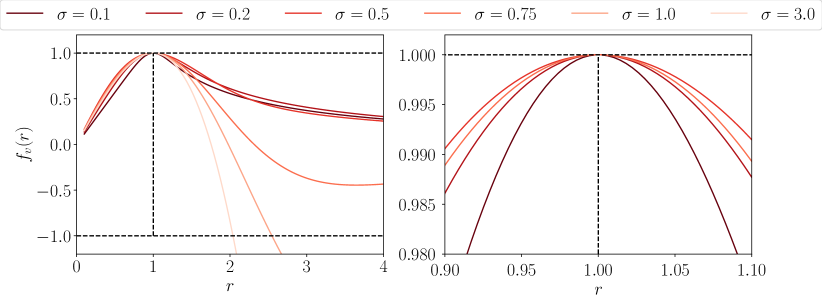
Figure 8: Graph of $f_{v}$ defined in 37 when $N=1$, $R_{1}=1$ and $\mathrm{sign}(a_{1})=1$ (left: global graph, right: zoom around $r=1$).

In Figure 9, we numerically compute $f_{v}^{\prime\prime}(R_{1})$ and notice it is (strictly) negative, even when ${\eta_{v}\notin\partial\mathrm{TV}(0)}$. This suggests that there exists ${\sigma_{0}>0}$ such that, for every ${\sigma\leq\sigma_{0}}$, the non-degenerate source condition holds (and, from our experiments, it seems that ${\sigma_{0}\geq 0.75}$). Surprisingly, $\sigma\mapsto f_{v}^{\prime\prime}(R_{1})$ does not seem to be monotonous, even on ${[0,\sigma_{0})}$.

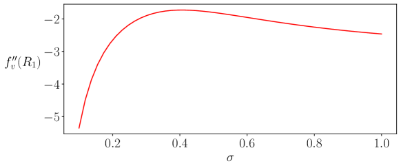
Figure 9: Graph of $f_{v}^{\prime\prime}(R_{1})$ as a function of $\sigma$ when $N=1$, $R_{1}=1$ and $\mathrm{sign}(a_{1})=1$.

Numerical experiments ($\bm{N\geq 2}$).

Now, we investigate the case where $N=2$. Our experiments suggest the existence of two completely different regimes. If $\mathrm{sign}(a_{1})\neq\mathrm{sign}(a_{2})$, then $\eta_{v}$ is non-degenerate only if $R_{1}$ and $R_{2}$ are not too close (see Figure 10). On the contrary, the case where $\mathrm{sign}(a_{1})=\mathrm{sign}(a_{2})$ seems to correspond to a real super-resolution regime, as $\eta_{v}$ is non-degenerate even for arbitrarily close $R_{1}$ and $R_{2}$ (see Figure 11). Still, we notice that, in this last case, the quantities $f_{v}^{\prime\prime}(R_{1})$ and $f_{v}^{\prime\prime}(R_{2})$, which control the stability of the recovery, go to $0$ as $R_{1}$ and $R_{2}$ get closer.

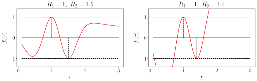
Figure 10: Graph of $f_{v}$ defined in 37 when $\sigma=0.2$, $N=2$, $\mathrm{sign}(a_{1})=-\mathrm{sign}(a_{2})$, $R_{1}=1$, ${R_{2}=1.5}$ (left) and $R_{2}=1.4$ (right).

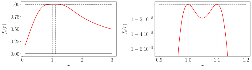
Figure 11: Graph of $f_{v}$ defined in 37 when $\sigma=0.2$, $N=2$, $\mathrm{sign}(a_{1})=\mathrm{sign}(a_{2})$, $R_{1}=1$ and ${R_{2}=1.1}$ (left: global graph, right: zoom around $1$).

Beyond the radial case.

In the general case, to numerically ensure that $\eta_{v}\in\partial\mathrm{TV}(0)$, one can solve

$$\underset{u\in\{\mathrm{TV}\leq 1\}}{\mathrm{sup}}~{}\int_{\mathbb{R}^{2}}\eta_{v}u\,,$$ (40)

which can be done by relying on standard discretization techniques. Indeed, as underlined in Section 3.1, we have that $\eta_{v}\in\partial\mathrm{TV}(0)$ if and only if 40 has a value which is no greater than $1$. To ensure the non-degenerate source condition holds, one must also show that ${|\int_{E}\eta_{v}|<P(E)}$ for every simple set $E$ such that $|E\triangle E_{i}|>0$ for every $i\in\{1,...,N\}$. This last property holds if and only if $\mathrm{Supp}(\mathrm{D}u)\subseteq\bigcup_{i=1}^{N}\partial E_{i}$ for every solution $u$ of 40. It can therefore be checked by finding, among all solutions of 40, the one such that $\mathrm{Supp}(\mathrm{D}u)$ is maximal.

Conclusion

We have showed that, in the low noise regime, the support of piecewise constant images can be exactly recovered from noisy linear measurements, provided that the measurement operator is smooth enough and some non-degenerate source condition holds. We have also provided numerical evidence that this last condition is satisfied for some radial images in the deconvolution setting. The investigation of its validity beyond the radial case, which we briefly discussed, is an interesting avenue for future research. It is also natural to wonder whether some quantitative version of our main result could be proved. This might be achieved by studying the stability of solutions to the prescribed curvature problem for non-smooth perturbations, possibly by adapting the selection principle of [Cicalese and Leonardi, 2012]. Finally, another direction could be to study the denoising case, which is not covered by our assumptions. In this setting, dual certificates are a priori non-smooth, which is a major source of difficulties.

Appendix A Proofs of Section 4

A.1 Proof of Proposition 4.1

We argue by contradiction and assume the existence of two sequences $(\eta_{n})_{n\in\mathbb{N}^{*}}$ and $(F_{n})_{n\in\mathbb{N}^{*}}$ such that

• for all $n\in\mathbb{N}^{*}$, $\eta_{n}\in\partial\mathrm{TV}(0)\cap\mathrm{C}^{1}(\mathbb{R}^{2})$,

• the sequence $(\eta_{n})_{n\in\mathbb{N}^{*}}$ converges to $\eta_{0}$ in $\mathrm{L}^{2}(\mathbb{R}^{2})$ and $\mathrm{C}^{1}(\mathbb{R}^{2})$,

• for all $n\in\mathbb{N}^{*}$, the set $F_{n}$ is a non-empty solution to ($\mathcal{PC}(\eta_{n})$) and cannot be written as a $\mathrm{C}^{2}$-normal deformation of size at most $\epsilon$ of a non-empty solution to ($\mathcal{PC}(\eta_{0})$) .

We hence have that $(F_{n})_{n\in\mathbb{N}^{*}}$ is bounded (by Lemma 2.8) and that $F_{n}$ is a strong $(\Lambda,r_{0})$-quasi minimizer of the perimeter (in short form ${F_{n}\in\mathcal{QM}(\Lambda,r_{0})}$, see [Maggi, 2012, Section 21] and [Ambrosio, 2010, Definition 4.7.3]) for all ${n\in\mathbb{N}^{*}}$, with $\Lambda=\mathrm{sup}\,\{\|\eta_{n}\|_{\infty},\,n\in\mathbb{N}^{*}\}$ and $r_{0}$ any positive real number. Taking $r_{0}$ small enough to have $\Lambda\,r_{0}\leq 1$, from [Maggi, 2012, Propositions 21.13 and 21.14] we get (up to the extraction of a not relabeled subsequence) that $(F_{n})_{n\in\mathbb{N}^{*}}$ converges in measure to a bounded set $E\in\mathcal{QM}(\Lambda,r_{0})$, and that $(\partial F_{n})_{n\in\mathbb{N}^{*}}$ converges to $\partial E$ in the Hausdorff sense. From $|F_{n}\triangle E|\to 0$ we obtain that $E$ is a solution to ($\mathcal{PC}(\eta_{0})$). In addition, since $F_{n}$ is non-empty for all $n$, using Lemma 2.8, we get that $E$ is non-empty. The convergence of $(\partial F_{n})_{n\in\mathbb{N}^{*}}$ towards $\partial E$ also yields

$$\forall r>0,~{}\exists n_{0}\in\mathbb{N},~{}\forall n\geq n_{0},~{}\partial F_{n}\subset\bigcup\limits_{x\in\partial E}C(x,r,\nu_{E}(x))\,,$$

where $C(x,r,\nu_{E}(x))$ denotes the square of axis $\nu_{E}(x)$ and side $r$ centered at $x$, defined in 2. From [Ambrosio, 2010, 4.7.4], and arguing as in the proof of [Maggi, 2012, Theorem 26.6], for every $x\in\partial E$ we obtain the existence of $r>0$, of $n_{0}\in\mathbb{N}$, of $u\in\mathrm{C}^{1,1}([-r,r])$ and of a sequence ${(u_{n})_{n\geq n_{0}}}$ which is uniformly bounded in $\mathrm{C}^{1,1}([-r,r])$, such that, in $C(x,r,\nu_{E}(x))$, the set $E$ is the hypograph of $u$ and, for every ${n\geq n_{0}}$, the set $F_{n}$ is the hypograph of $u_{n}$. Moreover, we have that $\|u_{n}-u\|_{\mathrm{C}^{1}([-r,r])}\to 0$.

Now, we also have that $u$ and $u_{n}$ (for $n\geq n_{0}$) respectively solve (in the sense of distributions) the following equations in $(-r,r)$:

$$\frac{u^{\prime\prime}(z)}{\left(1+u^{\prime}(z)^{2}\right)^{3/2}} =H(z,u(z))\,, \mathrm{with}~{}H(z,t) \stackrel{{\scriptstyle\mbox{\tiny def.}}}{{=}}\eta_{0}(x+R_{\nu_{E}(x)}(z,t))\,,$$ (41)

$$\frac{u_{n}^{\prime\prime}(z)}{\left(1+u_{n}^{\prime}(z)^{2}\right)^{3/2}} =H_{n}(z,u_{n}(z))\,, \mathrm{with}~{}H_{n}(z,t) \stackrel{{\scriptstyle\mbox{\tiny def.}}}{{=}}\eta_{n}(x+R_{\nu_{E}(x)}(z,t))\,.$$

We hence immediately obtain that $u$ and $u_{n}$ belong to $\mathrm{C}^{2}([-r,r])$. Moreover, for every $z\in(-r,r)$ we have:

$$|u^{\prime\prime}_{n}(z)-u^{\prime\prime}(z)| =\Big{|}H_{n}(z,u_{n}(z))\left(1+u^{\prime}_{n}(z)^{2}\right)^{3/2}-H(z,u(z))\left(1+u^{\prime}(z)^{2}\right)^{3/2}\Big{|}$$

$$\leq~{}~{}~{}~{}(\|H_{n}-H\|_{\infty}+|H(z,u_{n}(z))-H(z,u(z))|)\left(1+u^{\prime}_{n}(z)^{2}\right)^{3/2}$$

$$~{}~{}~{}~{}\,+\|H\|_{\infty}\left[\left(1+u^{\prime}_{n}(z)^{2}\right)^{3/2}-\left(1+u^{\prime}(z)^{2}\right)^{3/2}\right],$$

from which we obtain that $\|u^{\prime\prime}_{n}-u^{\prime\prime}\|_{\infty}\to 0$.

Using these new results in combination with 41, we get that $u$ and $u_{n}$ belong to $\mathrm{C}^{3}([-r,r])$. Differentiating 41, we obtain, for every $z\in(-r,r)$:

$$u^{(3)}(z) =~{}~{}~{}~{}\big{[}\partial_{1}H(z,u(z))+u^{\prime}(z)\,\partial_{2}H(z,u(z))\big{]}\,(1+u^{\prime}(z)^{2})^{3/2}$$

$$~{}~{}~{}~{}\,+3\,H(z,u(z))\,u^{\prime\prime}(z)\,u^{\prime}(z)\,(1+u^{\prime}(z)^{2})^{3/2}\,,$$

$$u_{n}^{(3)}(z) =~{}~{}~{}~{}\big{[}\partial_{1}H_{n}(z,u_{n}(z))+u^{\prime}_{n}(z)\,\partial_{2}H_{n}(z,u_{n}(z))\big{]}\,(1+u^{\prime}_{n}(z)^{2})^{3/2}$$

$$~{}~{}~{}~{}\,+3\,H_{n}(z,u_{n}(z))\,u^{\prime\prime}_{n}(z)\,u^{\prime}_{n}(z)\,(1+u^{\prime}_{n}(z)^{2})^{3/2}\,,$$

from which we can finally show $\|u^{(3)}_{n}-u^{(3)}\|_{\infty}\to 0$.

Finally, using the compactness of $\partial E$, we obtain that $(F_{n})_{n\geq 0}$ converges in $\mathrm{C}^{3}$ towards $E$, and Proposition 2.4 allows to eventually write $F_{n}$ as a $\mathrm{C}^{2}$-normal deformation of $E$, whose norm converges to zero. This yields a contradiction.

A.2 Proofs of Section 4.1

To prove Propositions 4.3 and 4.4, we need to compute $\mathrm{j}^{\prime\prime}_{E}(\varphi)$ for $\varphi\in\mathrm{C}^{1}(\partial E)$ in a neighborhood of $0$. This may be done using Lemma A.1 below. To state it, given a bounded set $E$ of class $\mathrm{C}^{2}$ and $\varphi$ in a neighborhood of $0$ in $\mathrm{C}^{1}(\partial E)$, we introduce the mapping $f_{\varphi}=Id+\xi_{\varphi}$, with $\xi_{\varphi}$ defined as in Lemma 2.2. If $\|\varphi\|_{\mathrm{C}^{1}(\partial E)}$ is sufficiently small then $f_{\varphi}$ is a $\mathrm{C}^{1}$-diffeomorphism, and we denote its inverse by $g_{\varphi}$.

Lemma A.1

Let $E$ be a bounded set of class $\mathrm{C}^{2}$. Then for every $\varphi$ in a neighborhood of $0$ in $\mathrm{C}^{1}(\partial E)$, and for every ${\psi\in\mathrm{H}^{1}(\partial E)}$, we have:

$$\mathrm{j}^{\prime\prime}_{E}(\varphi).(\psi,\psi)=j^{\prime\prime}_{E_{\varphi}}(0).(\xi_{\psi}\circ g_{\varphi}\cdot\nu_{\varphi},\,\xi_{\psi}\circ g_{\varphi}\cdot\nu_{\varphi})+\mathrm{j}^{\prime}_{E_{\varphi}}(0).(Z_{\varphi,\psi})$$ (42)

where $\nu_{\varphi}$ is the unit outward normal to $E_{\varphi}$ and

$$Z_{\varphi,\psi}=B_{\varphi}((\xi_{\psi}\circ g_{\varphi})_{\tau_{\varphi}},(\xi_{\psi}\circ g_{\varphi})_{\tau_{\varphi}})-2(\nabla_{\tau_{\varphi}}(\xi_{\psi}\circ g_{\varphi}\cdot\nu_{\varphi}))\cdot(\xi_{\psi}\circ g_{\varphi})_{\tau_{\varphi}}\,,$$

with $\zeta_{\tau_{\varphi}}$ and $\nabla_{\tau_{\varphi}}\zeta$ the tangential part and the tangential gradient of $\zeta$ with respect to $E_{\varphi}$, and $B_{\varphi}$ the second fundamental form of $E_{\varphi}$.

Proof.

To prove this result, we need to introduce $\mathcal{J}_{E}$ defined by

$$\!\begin{aligned} \mathcal{J}_{E}:\mathrm{C}^{1}_{b}(\mathbb{R}^{2},\mathbb{R}^{2})&\to\mathbb{R}\\ \xi&\mapsto J((Id+\xi)(E))\,.\end{aligned}$$

We denote by $\nu$ the outward unit normal to $E$ and $B$ its second fundamental form. We also denote $\zeta_{\tau}$ and $\nabla_{\tau}\zeta$ the tangential part and the tangential gradient of $\zeta$ with respect to $E$. The structure theorem (see e.g. [Henrot and Pierre, 2018, Theorem 5.9.2] or [Dambrine and Lamboley, 2019, Theorem 2.1]) then yields, for every sufficiently smooth vector field $\zeta$:

$$\mathcal{J}^{\prime}_{E}(0).(\zeta) =\mathrm{j}_{E}^{\prime}(0).(\mathchoice{{\zeta\,\smash{\vrule height=5.55557pt,depth=1.65279pt}}_{\,\partial E}}{{\zeta\,\smash{\vrule height=5.55557pt,depth=1.65279pt}}_{\,\partial E}}{{\zeta\,\smash{\vrule height=3.88889pt,depth=1.18056pt}}_{\,\partial E}}{{\zeta\,\smash{\vrule height=2.77777pt,depth=1.18056pt}}_{\,\partial E}}\cdot\nu)\,,$$

$$\mathcal{J}^{\prime\prime}_{E}(0).(\zeta,\zeta) =\mathrm{j}_{E}^{\prime\prime}(0).(\mathchoice{{\zeta\,\smash{\vrule height=5.55557pt,depth=1.65279pt}}_{\,\partial E}}{{\zeta\,\smash{\vrule height=5.55557pt,depth=1.65279pt}}_{\,\partial E}}{{\zeta\,\smash{\vrule height=3.88889pt,depth=1.18056pt}}_{\,\partial E}}{{\zeta\,\smash{\vrule height=2.77777pt,depth=1.18056pt}}_{\,\partial E}}\cdot\nu,\mathchoice{{\zeta\,\smash{\vrule height=5.55557pt,depth=1.65279pt}}_{\,\partial E}}{{\zeta\,\smash{\vrule height=5.55557pt,depth=1.65279pt}}_{\,\partial E}}{{\zeta\,\smash{\vrule height=3.88889pt,depth=1.18056pt}}_{\,\partial E}}{{\zeta\,\smash{\vrule height=2.77777pt,depth=1.18056pt}}_{\,\partial E}}\cdot\nu)+\mathrm{j}_{E}^{\prime}(0).(Z_{\zeta})\,,$$

where

$$Z_{\zeta}\stackrel{{\scriptstyle\mbox{\tiny def.}}}{{=}}B(\zeta_{\tau},\zeta_{\tau})-2\,(\nabla_{\tau}(\zeta\cdot\nu))\cdot\zeta_{\tau}\,.$$

Now, we first notice that, for every pair of vector fields $\xi,\zeta$ such that $Id+\xi$ is invertible, we have:

$$(Id+\xi+\zeta)(E)=(Id+\zeta\circ(Id+\xi)^{-1})((Id+\xi)(E))\,.$$

Defining $F\stackrel{{\scriptstyle\mbox{\tiny def.}}}{{=}}(Id+\xi)(E)$ we hence obtain $\mathcal{J}_{E}(\xi+\zeta)=\mathcal{J}_{F}(\zeta\circ(Id+\xi)^{-1},\zeta\circ(Id+\xi)^{-1})$, which yields

$$\mathcal{J}^{\prime\prime}_{E}(\xi).(\zeta,\zeta)=\mathcal{J}_{F}^{\prime\prime}(0).(\zeta\circ(Id+\xi)^{-1})\,.$$

Using this with $\xi=\xi_{\varphi}$ and $\zeta=\xi_{\psi}$, we get:

$$\mathrm{j}_{E}^{\prime\prime}(\varphi).(\psi,\psi)=\mathcal{J}^{\prime\prime}_{E}(\xi_{\varphi})(\xi_{\psi},\xi_{\psi})=\mathcal{J}^{\prime\prime}_{E_{\varphi}}(0).(\xi_{\psi}\circ g_{\varphi},\xi_{\psi}\circ g_{\varphi})\,,$$

and we finally obtain 42 by applying the structure theorem. ∎

Most of the results below rely on the following technical lemma, whose first part is contained in [Dambrine and Lamboley, 2019, Lemma 4.7].

Lemma A.2

Let $E$ be a bounded $\mathrm{C}^{2}$ set. If $\|\varphi\|_{\mathrm{C}^{1}(\partial E)}\to 0$ we have:

$$(i) \|f_{\varphi}-Id\|_{\mathrm{C}^{1}(\partial E)}\to 0\,, \|\nu_{\varphi}\circ f_{\varphi}-\nu\|_{\mathrm{C}^{0}(\partial E)}\to 0\,, (iii)$$

$$(ii) \|g_{\varphi}-Id\|_{\mathrm{C}^{1}(\partial E_{\varphi})}\to 0\,, \|\mathrm{Jac}_{\tau}f_{\varphi}-1\|_{\mathrm{C}^{0}(\partial E)}\to 0\,. (iv)$$

If $\|\varphi\|_{\mathrm{C}^{2}(\partial E)}\to 0$ then we also have:

$$(v) \|H_{\varphi}\circ f_{\varphi}-H\|_{\mathrm{C}^{0}(\partial E)}\to 0\,, \|B_{\varphi}\circ f_{\varphi}-B\|_{\mathrm{C}^{0}(\partial E)}\to 0\,. (vi)$$

Moreover, the following holds:

$$(a){}{} \underset{\|\varphi\|_{\mathrm{C}^{1}(\partial E)}\to 0}{\mathrm{lim}}~{}\underset{\psi\in\mathrm{L}^{2}(\partial E)\setminus\{0\}}{\mathrm{sup}}~{}\frac{\|(\xi_{\psi}\circ g_{\varphi})_{\tau_{\varphi}}\|_{\mathrm{L}^{2}(\partial E_{\varphi})}}{\|\psi\|_{\mathrm{L}^{2}(\partial E)}}=0\,,$$

$$(b){}{} \underset{\|\varphi\|_{\mathrm{C}^{1}(\partial E)}\to 0}{\mathrm{lim}}~{}\underset{\psi\in\mathrm{H}^{1}(\partial E)\setminus\{0\}}{\mathrm{sup}}\frac{\left|\|\nabla_{\tau_{\varphi}}(\xi_{\psi}\circ g_{\varphi}\cdot\nu_{\varphi})\|_{\mathrm{L}^{2}(\partial E_{\varphi})}-\|\nabla_{\tau}\psi\|_{\mathrm{L}^{2}(\partial E)}\right|}{\|\psi\|_{\mathrm{H}^{1}(\partial E)}}=0\,,$$

$$(c){}{} \underset{\|\varphi\|_{\mathrm{C}^{2}(\partial E)}\to 0}{\mathrm{lim}}~{}\underset{\psi\in\mathrm{H}^{1}(\partial E)\setminus\{0\}}{\mathrm{sup}}\frac{\|Z_{\varphi,\psi}\|_{\mathrm{L}^{1}(\partial E_{\varphi})}}{\|\psi\|_{\mathrm{H}^{1}(\partial E)}^{2}}=0\,.$$

Proof.

See [Dambrine and Lamboley, 2019, Lemma 4.7] for a proof of the results stated in the first part of the lemma. To prove $(a)$ we use the fact that

$$\|(\xi_{\psi}\circ g_{\varphi})_{\tau_{\varphi}}\|_{\mathrm{L}^{2}(\partial E_{\varphi})}^{2} =\int_{\partial E}(\nu\circ g_{\varphi})^{2}_{\tau_{\varphi}}\circ f_{\varphi}~{}\mathrm{Jac}_{\tau}f_{\varphi}\,\psi^{2}\,d\mathcal{H}^{1}$$

$$\leq\|\mathrm{Jac}_{\tau}f_{\varphi}\|_{\mathrm{C}^{0}(\partial E)}\,\|(\nu\circ g_{\varphi})_{\tau_{\varphi}}\circ f_{\varphi}\|_{\mathrm{C}^{0}(\partial E)}^{2}\,\|\psi\|_{\mathrm{L}^{2}(\partial E)}^{2}$$

$$=\|\mathrm{Jac}_{\tau}f_{\varphi}\|_{\mathrm{C}^{0}(\partial E)}\,\|\nu-(\nu\cdot\nu_{\varphi}\circ f_{\varphi})\,\nu_{\varphi}\circ f_{\varphi}\|_{\mathrm{C}^{0}(\partial E)}^{2}\,\|\psi\|_{\mathrm{L}^{2}(\partial E)}^{2}\,.$$

which, using $(i)$, $(iii)$ and $(iv)$, yields the result.

To prove $(b)$, we notice that:

$$\nabla_{\tau_{\varphi}}(\xi_{\psi}\circ g_{\varphi}\cdot\nu_{\varphi}) =\left[c^{1}_{\varphi}\,\psi\circ g_{\varphi}+c^{2}_{\varphi}\cdot\nabla_{\tau}\psi\circ g_{\varphi}\right]\tau_{\varphi}\,,$$

with $\tau=\nu^{\perp}$, $\tau_{\varphi}=\nu_{\varphi}^{\perp}$ and

$$c^{1}_{\varphi}\stackrel{{\scriptstyle\mbox{\tiny def.}}}{{=}}\tau\circ g_{\varphi}\cdot\nu_{\varphi}~{}(J_{g_{\varphi}}\,\tau_{\varphi})\cdot\tau\circ g_{\varphi}+\tau_{\varphi}\cdot\nu\circ g_{\varphi}\,,~{}~{}~{}~{}~{}~{}c^{2}_{\varphi}\stackrel{{\scriptstyle\mbox{\tiny def.}}}{{=}}\nu\circ g_{\varphi}\cdot\nu_{\varphi}~{}(J_{g_{\varphi}}\,\tau_{\varphi})\,.$$

We hence obtain

$$|\nabla_{\tau_{\varphi}}(\xi_{\psi}\circ g_{\varphi}\cdot\nu_{\varphi})\circ f_{\varphi}\,\mathrm{Jac}_{\tau}f_{\varphi}-\nabla_{\tau}\psi|\leq c_{\varphi}\,(|\psi|+|\nabla_{\tau}\psi|)$$

with $c_{\varphi}$ independant of $\psi$. Moreover, using $(ii)$ and $(iii)$, we have:

$$\underset{\|\varphi\|_{\mathrm{C}^{1}(\partial E)}\to 0}{\mathrm{lim}}~{}\|c_{\varphi}\|_{\mathrm{C}^{0}(\partial E)}\to 0\,.$$

Denoting $\mathcal{A}\stackrel{{\scriptstyle\mbox{\tiny def.}}}{{=}}\left|\|\nabla_{\tau_{\varphi}}(\xi_{\psi}\circ g_{\varphi}\cdot\nu_{\varphi})\|_{\mathrm{L}^{2}(\partial E_{\varphi})}-\|\nabla_{\tau}\psi\|_{\mathrm{L}^{2}(\partial E)}\right|$, this finally yields

$$\mathcal{A} \leq\|\nabla_{\tau_{\varphi}}(\xi_{\psi}\circ g_{\varphi}\cdot\nu_{\varphi})\circ f_{\varphi}\,\mathrm{Jac}_{\tau}f_{\varphi}-\nabla_{\tau}\psi\|_{\mathrm{L}^{2}(\partial E)}$$

$$\leq\sqrt{2}~{}\|c_{\varphi}\|_{\mathrm{C}^{0}(\partial E)}\,\|\psi\|_{\mathrm{H}^{1}(\partial E)}\,.$$

We now prove $(c)$. Since

$$\|B_{\varphi}((\xi_{\psi}\circ g_{\varphi})_{\tau_{\varphi}},(\xi_{\psi}\circ g_{\varphi})_{\tau_{\varphi}})\|_{\mathrm{L}^{1}(\partial E_{\varphi})} \leq\|B_{\varphi}\|_{\mathrm{C}^{0}(\partial E_{\varphi})}\,\|(\xi_{\psi}\circ g_{\varphi})_{\tau_{\varphi}}\|_{\mathrm{L}^{2}(\partial E_{\varphi})}^{2}$$

and

$$\mathcal{B} \leq\|\nabla_{\tau_{\varphi}}(\xi_{\psi}\circ g_{\varphi}\cdot\nu_{\varphi}))\|_{\mathrm{L}^{2}(\partial E_{\varphi})}\,\|(\xi_{\psi}\circ g_{\varphi})_{\tau_{\varphi}}\|_{\mathrm{L}^{2}(\partial E_{\varphi})}$$

with $\mathcal{B}\stackrel{{\scriptstyle\mbox{\tiny def.}}}{{=}}\|(\nabla_{\tau_{\varphi}}(\xi_{\psi}\circ g_{\varphi}\cdot\nu_{\varphi}))\cdot(\xi_{\psi}\circ g_{\varphi})_{\tau_{\varphi}}\|_{\mathrm{L}^{1}(\partial E_{\varphi})}$, we get the result. ∎

Using the above result, we now prove the continuity of $\varphi\mapsto\mathrm{j}^{\prime\prime}_{E}(\varphi)$ by proving the continuity of the two terms appearing in its expression. We recall that, if $E$ is a (real) vector space, we denote by $\mathcal{Q}(E)$ the set of quadratic forms over $E$.

Proposition A.3

If $E$ is a bounded $\mathrm{C}^{2}$ set and $\mathrm{p}_{E}:\varphi\mapsto P(E_{\varphi})$, the mapping

$$\!\begin{aligned} \mathrm{p}^{\prime\prime}_{E}:\mathrm{C}^{2}(\partial E)&\to\mathcal{Q}(\mathrm{H}^{1}(\partial E))\\ \varphi&\mapsto\mathrm{p}^{\prime\prime}_{E}(\varphi)\end{aligned}$$

is continuous at $0$.

Proof.

Using Lemma A.2, for every $\varphi\in\mathrm{C}^{2}(\partial E)$ in a neighborhood of $0$ and $\psi\in\mathrm{H}^{1}(\partial E)$, we obtain:

$$\mathrm{p}^{\prime\prime}_{E}(\varphi).(\psi,\psi)-\mathrm{p}^{\prime\prime}_{E}(0).(\psi,\psi)=\mathcal{A}+\mathrm{p}^{\prime}_{E_{\varphi}}(0).(Z_{\varphi,\psi})\,,$$

with $\mathcal{A}\stackrel{{\scriptstyle\mbox{\tiny def.}}}{{=}}\mathrm{p}^{\prime\prime}_{E_{\varphi}}(0).((\xi_{\psi}\circ g_{\varphi})\cdot\nu_{\varphi},(\xi_{\psi}\circ g_{\varphi})\cdot\nu_{\varphi})-\mathrm{p}^{\prime\prime}_{E}(0).(\psi,\psi)$. Now, we also have:

$$\mathcal{A}=\|\nabla_{\tau_{\varphi}}(\xi_{\psi}\circ g_{\varphi}\cdot\nu_{\varphi})\|_{\mathrm{L}^{2}(\partial E_{\varphi})}^{2}-\|\nabla_{\tau}\psi\|_{\mathrm{L}^{2}(\partial E)}^{2}\,,$$

and using Lemma A.2 we obtain

$$\underset{\|\varphi\|_{\mathrm{C}^{2}(\partial E)}\to 0}{\mathrm{lim}}~{}\underset{\psi\in\mathrm{H}^{1}(\partial E)\setminus\{0\}}{\mathrm{sup}}\frac{\left|\mathrm{p}^{\prime\prime}_{E_{\varphi}}(0).((\xi_{\psi}\circ g_{\varphi})\cdot\nu_{E_{\varphi}},(\xi_{\psi}\circ g_{\varphi})\cdot\nu_{E_{\varphi}})-\mathrm{p}^{\prime\prime}_{E}(0).(\psi,\psi)\right|}{\|\psi\|_{\mathrm{H}^{1}(\partial E)}^{2}}=0\,.$$

Moreover

$$|\mathrm{p}^{\prime}_{E}(0).(Z_{\varphi,\psi})| \leq\|H_{\varphi}\|_{\mathrm{L}^{\infty}(\partial E_{\varphi})}\,\|Z_{\varphi,\psi}\|_{\mathrm{L}^{1}(\partial E_{\varphi})}\,,$$

and Lemma A.2 allows to conclude. ∎

Proposition A.4

If $E$ is a bounded $\mathrm{C}^{2}$ set, $\eta\in\mathrm{C}^{1}(\mathbb{R}^{2})$ and $\mathrm{g}_{E}:\varphi\mapsto\int_{E_{\varphi}}\eta$, the mapping

$$\!\begin{aligned} \mathrm{g}^{\prime\prime}_{E}:\mathrm{C}^{2}(\partial E)&\to\mathcal{Q}(\mathrm{H}^{1}(\partial E))\\ \varphi&\mapsto\mathrm{g}^{\prime\prime}_{E}(\varphi)\end{aligned}$$

is continuous at $0$.

Proof.

We proceed as in Proposition A.3. Defining

$$\mathcal{A}\stackrel{{\scriptstyle\mbox{\tiny def.}}}{{=}}\mathrm{g}^{\prime\prime}_{E_{\varphi}}(0).((\xi_{\psi}\circ g_{\varphi})\cdot\nu_{E_{\varphi}},(\xi_{\psi}\circ g_{\varphi})\cdot\nu_{E_{\varphi}})$$

we have:

$$\mathcal{A} =\int_{\partial E_{\varphi}}\left[H_{\varphi}\,\eta+\frac{\partial\eta}{\partial\nu_{\varphi}}\right]((\psi\,\nu)\circ g_{\varphi}\cdot\nu_{E_{\varphi}})^{2}\,d\mathcal{H}^{1}$$

$$=\int_{\partial E}\left[H_{\varphi}\,\eta+\frac{\partial\eta}{\partial\nu_{\varphi}}\right]\circ f_{\varphi}\,(\nu\cdot\nu_{\varphi}\circ f_{\varphi})^{2}\,\mathrm{Jac}_{\tau}f_{\varphi}\,\psi^{2}\,d\mathcal{H}^{1}.$$

This yields:

$$\frac{\left|\mathrm{g}^{\prime\prime}_{E_{\varphi}}(0).((\xi_{\psi}\circ g_{\varphi})\cdot\nu_{\varphi},(\xi_{\psi}\circ g_{\varphi})\cdot\nu_{\varphi})-\mathrm{g}^{\prime\prime}_{E}(0).(\psi,\psi)\right|}{\|\psi\|_{\mathrm{L}^{2}(\partial E)}^{2}}\leq c_{\varphi}\,,$$

with

$$c_{\varphi}\stackrel{{\scriptstyle\mbox{\tiny def.}}}{{=}}\left\|\left[H_{\varphi}\,\eta+\frac{\partial\eta}{\partial\nu_{\varphi}}\right]\circ f_{\varphi}\,(\nu\cdot\nu_{\varphi}\circ f_{\varphi})^{2}\,\mathrm{Jac}_{\tau}f_{\varphi}-\left[H\,\eta+\frac{\partial\eta}{\partial\nu}\right]\right\|_{\infty}.$$

Using Lemma A.2 we obtain

$$\underset{\|\varphi\|_{\mathrm{C}^{2}(\partial E)\to 0}}{\mathrm{lim}}~{}\underset{\psi\in\mathrm{H}^{1}(\partial E)\setminus\{0\}}{\mathrm{sup}}\frac{\left|\mathrm{g}^{\prime\prime}_{E_{\varphi}}(0).((\xi_{\psi}\circ g_{\varphi})\cdot\nu_{\varphi},(\xi_{\psi}\circ g_{\varphi})\cdot\nu_{\varphi})-\mathrm{g}^{\prime\prime}_{E}(0).(\psi,\psi)\right|}{\|\psi\|_{\mathrm{H}^{1}(\partial E)}^{2}}=0\,.$$

Moreover

$$|\mathrm{g}^{\prime}_{E_{\varphi}}(0).(Z_{\varphi,\psi})| \leq\|\eta\|_{\infty}\,\|Z_{\varphi,\psi}\|_{\mathrm{L}^{1}(\partial E_{\varphi})}\,,$$

and using again Lemma A.2 we finally obtain the result. ∎

Proof of Proposition 4.4:

Proof.

Since $\left|(\mathrm{j}_{E}-\mathrm{j}_{0,E})^{\prime\prime}(\varphi).(\psi,\psi)\right|\leq c^{1}_{\varphi}+c^{2}_{\varphi}$ with

$$c^{1}_{\varphi} \stackrel{{\scriptstyle\mbox{\tiny def.}}}{{=}}\left|\int_{\partial E_{\varphi}}\left(H_{\varphi}\,(\eta-\eta_{0})+\frac{\partial\,(\eta-\eta_{0})}{\partial\nu_{\varphi}}\right)(\xi_{\psi}\circ g_{\varphi}\cdot\nu_{\varphi})^{2}\,d\mathcal{H}^{1}\right|,$$

$$c^{2}_{\varphi} \stackrel{{\scriptstyle\mbox{\tiny def.}}}{{=}}\left|\int_{\partial E_{\varphi}}(\eta-\eta_{0})\,Z_{\varphi,\psi}\,d\mathcal{H}^{1}\right|,$$

the result readily follows from Lemma A.2. ∎

References

- [Acar and Vogel, 1994] Acar, R. and Vogel, C. R. (1994). Analysis of bounded variation penalty methods for ill-posed problems. Inverse Problems, 10(6):1217.
- [Allard, 2008a] Allard, W. K. (2008a). Total Variation Regularization for Image Denoising, I. Geometric Theory. SIAM Journal on Mathematical Analysis, 39(4):1150–1190. Publisher: Society for Industrial and Applied Mathematics.
- [Allard, 2008b] Allard, W. K. (2008b). Total Variation Regularization for Image Denoising, II. Examples. SIAM Journal on Imaging Sciences, 1(4):400–417. Publisher: Society for Industrial and Applied Mathematics.
- [Allard, 2009] Allard, W. K. (2009). Total Variation Regularization for Image Denoising, III. Examples. SIAM Journal on Imaging Sciences, 2(2):532–568. Publisher: Society for Industrial and Applied Mathematics.
- [Alter and Caselles, 2009] Alter, F. and Caselles, V. (2009). Uniqueness of the Cheeger set of a convex body. Nonlinear Analysis: Theory, Methods & Applications, 70(1):32–44.
- [Alter et al., 2005a] Alter, F., Caselles, V., and Chambolle, A. (2005a). A characterization of convex calibrable sets in Rn. Mathematische Annalen, 332(2):329–366.
- [Alter et al., 2005b] Alter, F., Caselles, V., and Chambolle, A. (2005b). Evolution of characteristic functions of convex sets in the plane by the minimizing total variation flow. Interfaces and Free Boundaries, 7(1):29–53.
- [Ambrosio, 2010] Ambrosio, L. (2010). Corso introduttivo alla teoria geometrica della misura e alle superfici minime. Scuola Normale Superiore.
- [Ambrosio et al., 2001] Ambrosio, L., Caselles, V., Masnou, S., and Morel, J.-M. (2001). Connected components of sets of finite perimeter and applications to image processing. Journal of the European Mathematical Society, 3(1):39–92.
- [Ambrosio et al., 2000] Ambrosio, L., Fusco, N., and Pallara, D. (2000). Functions of Bounded Variation and Free Discontinuity Problems. Oxford Mathematical Monographs. Oxford University Press, Oxford, New York.
- [Aujol et al., 2005] Aujol, J.-F., Aubert, G., Blanc-Féraud, L., and Chambolle, A. (2005). Image Decomposition into a Bounded Variation Component and an Oscillating Component. Journal of Mathematical Imaging and Vision, 22(1):71–88.
- [Azaïs et al., 2015] Azaïs, J.-M., de Castro, Y., and Gamboa, F. (2015). Spike detection from inaccurate samplings. Applied and Computational Harmonic Analysis, 38(2):177–195.
- [Bach, 2013] Bach, F. (2013). Learning with Submodular Functions: A Convex Optimization Perspective. Foundations and Trends® in Machine Learning, 6(2-3):145–373.
- [Bellettini et al., 2002] Bellettini, G., Caselles, V., and Novaga, M. (2002). The Total Variation Flow in RN. Journal of Differential Equations, 184(2):475–525.
- [Boyer et al., 2019] Boyer, C., Chambolle, A., De Castro, Y., Duval, V., De Gournay, F., and Weiss, P. (2019). On Representer Theorems and Convex Regularization. SIAM Journal on Optimization, 29(2):1260–1281.
- [Boyer et al., 2023] Boyer, C., Chambolle, A., De Castro, Y., Duval, V., De Gournay, F., and Weiss, P. (2023). in preparation.
- [Bredies and Carioni, 2019] Bredies, K. and Carioni, M. (2019). Sparsity of solutions for variational inverse problems with finite-dimensional data. Calculus of Variations and Partial Differential Equations, 59(1):14.
- [Bredies and Pikkarainen, 2013] Bredies, K. and Pikkarainen, H. K. (2013). Inverse problems in spaces of measures. ESAIM: Control, Optimisation and Calculus of Variations, 19(1):190–218.
- [Bredies and Vicente, 2019] Bredies, K. and Vicente, D. (2019). A perfect reconstruction property for PDE-constrained total-variation minimization with application in Quantitative Susceptibility Mapping. ESAIM: Control, Optimisation and Calculus of Variations, 25:83.
- [Burger and Osher, 2004] Burger, M. and Osher, S. (2004). Convergence rates of convex variational regularization. Inverse Problems, 20(5):1411–1421.
- [Candès and Fernandez-Granda, 2014] Candès, E. J. and Fernandez-Granda, C. (2014). Towards a Mathematical Theory of Super-resolution. Communications on Pure and Applied Mathematics, 67(6):906–956.
- [Caselles et al., 2007] Caselles, V., Chambolle, A., and Novaga, M. (2007). The Discontinuity Set of Solutions of the TV Denoising Problem and Some Extensions. Multiscale Modeling & Simulation, 6(3):879–894.
- [Chambolle et al., 2010] Chambolle, A., Caselles, V., Cremers, D., Novaga, M., and Pock, T. (2010). An Introduction to Total Variation for Image Analysis. In An Introduction to Total Variation for Image Analysis, pages 263–340. De Gruyter.
- [Chambolle et al., 2016] Chambolle, A., Duval, V., Peyré, G., and Poon, C. (2016). Geometric properties of solutions to the total variation denoising problem. Inverse Problems, 33(1):015002.
- [Chambolle and Lions, 1997] Chambolle, A. and Lions, P.-L. (1997). Image recovery via total variation minimization and related problems. Numerische Mathematik, 76(2):167–188.
- [Chavent and Kunisch, 1997] Chavent, G. and Kunisch, K. (1997). Regularization of linear least squares problems by total bounded variation. ESAIM: Control, Optimisation and Calculus of Variations, 2:359–376.
- [Chen et al., 1998] Chen, S. S., Donoho, D. L., and Saunders, M. A. (1998). Atomic decomposition by basis pursuit. SIAM Journal on Scientific Computing, 20(1):33–61.
- [Cicalese and Leonardi, 2012] Cicalese, M. and Leonardi, G. P. (2012). A Selection Principle for the Sharp Quantitative Isoperimetric Inequality. Archive for Rational Mechanics and Analysis, 206(2):617–643.
- [Condat, 2017] Condat, L. (2017). Discrete Total Variation: New Definition and Minimization. SIAM Journal on Imaging Sciences, 10(3):1258–1290. Publisher: Society for Industrial and Applied Mathematics.
- [Cristoferi and Fonseca, 2019] Cristoferi, R. and Fonseca, I. (2019). Piecewise constant reconstruction of damaged color images. ESAIM: Control, Optimisation and Calculus of Variations, 25:37.
- [Dambrine and Lamboley, 2019] Dambrine, M. and Lamboley, J. (2019). Stability in shape optimization with second variation. Journal of Differential Equations, 267(5):3009–3045.
- [De Castro and Gamboa, 2012] De Castro, Y. and Gamboa, F. (2012). Exact reconstruction using Beurling minimal extrapolation. Journal of Mathematical Analysis and Applications, 395(1):336–354.
- [Delfour and Zolesio, 2011] Delfour, M. C. and Zolesio, J.-P. (2011). Shapes and Geometries: Metrics, Analysis, Differential Calculus, and Optimization, Second Edition. SIAM.
- [Duval, 2022] Duval, V. (2022). Faces and Extreme Points of Convex Sets for the Resolution of Inverse Problems. Habilitation à diriger des recherches, Université Paris Dauphine - PSL.
- [Duval and Peyré, 2015] Duval, V. and Peyré, G. (2015). Exact Support Recovery for Sparse Spikes Deconvolution. Foundations of Computational Mathematics, 15(5):1315–1355.
- [Engl et al., 1996] Engl, H., Hanke, M., and Neubauer, A. (1996). Regularization of Inverse Problems. Mathematics and Its Applications. Springer Netherlands.
- [Fleming, 1957] Fleming, W. H. (1957). Functions with generalized gradient and generalized surfaces. Annali di Matematica Pura ed Applicata, 44(1):93–103.
- [Fonseca et al., 2010] Fonseca, I., Leoni, G., Maggi, F., and Morini, M. (2010). Exact reconstruction of damaged color images using a total variation model. Annales de l’IHP Analyse non linéaire, 27(5):1291–1331.
- [Fornasier, 2006] Fornasier, M. (2006). Nonlinear projection recovery in digital inpainting for color image restoration. Journal of Mathematical Imaging and Vision, 24:359–373.
- [Fornasier and March, 2007] Fornasier, M. and March, R. (2007). Restoration of color images by vector valued bv functions and variational calculus. SIAM Journal on Applied Mathematics, 68(2):437–460.
- [Fujishige, 2005] Fujishige, S. (2005). Submodular Functions and Optimization. Elsevier.
- [Gonzales et al., 1993] Gonzales, E. H. A., Massari, U., and Tamanini, I. (1993). Boundaries of prescribed mean curvature. Atti della Accademia Nazionale dei Lincei. Classe di Scienze Fisiche, Matematiche e Naturali. Rendiconti Lincei. Matematica e Applicazioni, 4(3):197–206.
- [Haddad, 2007] Haddad, A. (2007). Texture Separation and Models. Multiscale Modeling & Simulation, 6(1):273–286. Publisher: Society for Industrial and Applied Mathematics.
- [Henrot and Pierre, 2018] Henrot, A. and Pierre, M. (2018). Shape Variation and Optimization : A Geometrical Analysis. Number 28 in Tracts in Mathematics. European Mathematical Society.
- [Hofmann et al., 2007] Hofmann, B., Kaltenbacher, B., Pöschl, C., and Scherzer, O. (2007). A convergence rates result for Tikhonov regularization in Banach spaces with non-smooth operators. Inverse Problems, 23(3):987–1010.
- [Holler and Wirth, 2022] Holler, M. and Wirth, B. (2022). Exact reconstruction and reconstruction from noisy data with anisotropic total variation.
- [Iglesias et al., 2018] Iglesias, J. A., Mercier, G., and Scherzer, O. (2018). A note on convergence of solutions of total variation regularized linear inverse problems. Inverse Problems, 34(5):055011.
- [Jalalzai, 2016] Jalalzai, K. (2016). Some Remarks on the Staircasing Phenomenon in Total Variation-Based Image Denoising. Journal of Mathematical Imaging and Vision, 54(2):256–268.
- [Kindermann et al., 2006] Kindermann, S., Osher, S., and Xu, J. (2006). Denoising by BV-duality. Journal of Scientific Computing, 28(2):411–444.
- [Kuttler and Sigillito, 1984] Kuttler, J. R. and Sigillito, V. G. (1984). Eigenvalues of the Laplacian in Two Dimensions. SIAM Review, 26(2):163–193.
- [Maggi, 2012] Maggi, F. (2012). Sets of Finite Perimeter and Geometric Variational Problems: An Introduction to Geometric Measure Theory. Cambridge Studies in Advanced Mathematics. Cambridge University Press, Cambridge.
- [Meyer, 2001] Meyer, Y. (2001). Oscillating Patterns in Image Processing and Nonlinear Evolution Equations: The Fifteenth Dean Jacqueline B. Lewis Memorial Lectures. American Mathematical Society, Boston, MA, USA.
- [Neubauer, 1989] Neubauer, A. (1989). Tikhonov regularisation for non-linear ill-posed problems: Optimal convergence rates and finite-dimensional approximation. Inverse Problems, 5(4):541.
- [Nikolova, 2000] Nikolova, M. (2000). Local Strong Homogeneity of a Regularized Estimator. SIAM Journal on Applied Mathematics, 61(2):633–658.
- [Poon et al., 2023] Poon, C., Keriven, N., and Peyré, G. (2023). The Geometry of Off-the-Grid Compressed Sensing. Foundations of Computational Mathematics, 23(1):241–327.
- [Poon and Peyré, 2019] Poon, C. and Peyré, G. (2019). Multi-dimensional Sparse Super-Resolution. SIAM Journal on Mathematical Analysis, 51(1):1–44.
- [Ring, 2000] Ring, W. (2000). Structural Properties of Solutions to Total Variation Regularization Problems. ESAIM: Mathematical Modelling and Numerical Analysis, 34(4):799–810.
- [Rockafellar, 1970] Rockafellar, R. T. (1970). Convex Analysis. Princeton University Press.
- [Rockafellar and Wets, 1998] Rockafellar, R. T. and Wets, R. J.-B. (1998). Variational Analysis. Grundlehren Der Mathematischen Wissenschaften. Springer-Verlag, Berlin Heidelberg.
- [Rudin et al., 1992] Rudin, L. I., Osher, S., and Fatemi, E. (1992). Nonlinear total variation based noise removal algorithms. Physica D: Nonlinear Phenomena, 60(1):259–268.
- [Tibshirani, 1996] Tibshirani, R. (1996). Regression Shrinkage and Selection Via the Lasso. Journal of the Royal Statistical Society: Series B (Methodological), 58(1):267–288.