\newsiamthm

claimClaim \newsiamremarkremarkRemark \newsiamremarkhypothesisHypothesis


\headersTikhonov Regularized Primal-Dual Dynamical MethodsT.T. ZHU, R. HU, and Y.P. FANG


Tikhonov regularized second-order plus first-order primal-dual dynamical systems with asymptotically vanishing damping for linear equality constrained convex optimization problemsthanks: The authors certify that the general content of the manuscript, in whole or in part, is not submitted, accepted, or published elsewhere, including conference proceedings. \fundingThis work was supported by the National Natural Science Foundation of China (11471230).

Ting Ting Zhu Department of Mathematics, Sichuan University, Chengdu, Sichuan, P.R. China (). zttsicuandaxue@126.com    Rong Hu Department of Applied Mathematics, Chengdu University of Information Technology, Chengdu, Sichuan, P.R. China (). ronghumath@aliyun.com    Ya Ping Fang Department of Mathematics, Sichuan University, Chengdu, Sichuan, P.R. China (, The corresponding author). ypfang@scu.edu.cn
Abstract

In this paper, in the setting of Hilbert spaces, we consider a Tikhonov regularized second-order plus first-order primal-dual dynamical system with asymptotically vanishing damping for a linear equality constrained convex optimization problem. The convergence properties of the proposed dynamical system depend heavily upon the choice of the Tikhonov regularization parameter. When the Tikhonov regularization parameter decreases rapidly to zero, we establish the fast convergence rates of the primal-dual gap, the objective function error, the feasibility measure, and the gradient norm of the objective function along the trajectory generated by the system. When the Tikhonov regularization parameter tends slowly to zero, we prove that the primal trajectory of the Tikhonov regularized dynamical system converges strongly to the minimal norm solution of the linear equality constrained convex optimization problem. Numerical experiments are performed to illustrate the efficiency of our approach.

keywords:
Linear equality constrained convex optimization problem, second-order plus first-order primal-dual dynamical system, asymptotically vanishing damping, Tikhonov regularization, convergence rate, strong convergence
{MSCcodes} 34D05, 37N40, 46N10, 90C25

1 Introduction

Let $\mathcal{X}$ and $\mathcal{Y}$ be two real Hilbert spaces which are endowed with the inner product $\langle\cdot,\cdot\rangle$ and the associated norm $\|\cdot\|$. Consider the linear equality constrained convex optimization problem

(1) minf(x), s.t. Ax=b,𝑓𝑥 s.t. 𝐴𝑥𝑏\min\quad f(x),\quad\text{ s.t. }\ Ax=b,

where $A:\mathcal{X}\rightarrow\mathcal{Y}$ is a continuous linear operator, $b\in\mathcal{Y}$, and $f:\mathcal{X}\rightarrow\mathbb{R}$ is a continuously differentiable convex function such that the gradient operator $\nabla f$ of $f$ is Lipschitz continuous. The problem (1) is a basic model for many important applications arising in various areas, such as machine learning [18, 33], image recovery [24], the energy dispatch of power grids [45, 46], network optimization [40, 47], and distributed optimization [35, 48]. When $A=0$ and $b=0$, the problem (1) reduces to the unconstrained optimization problem

(2) minf(x).𝑓𝑥\min\quad f(x).

In the literature there has been a flurry of research on second-order dynamical systems for the unconstrained optimization problem (2). A seminal work is due to Polyak [38] who proposed the heavy ball with friction system

$\displaystyle\ddot{x}(t)+\gamma\dot{x}(t)+\nabla f(x(t))=0,\qquad\qquad\text{(HBF)}$

where the damping coefficient $\gamma>0$ is a constant. Another seminal work is due to Su, Boyd, and Cand$\grave{e}$s [41] who proposed the asymptotically vanishing damping inertial dynamical system

$\displaystyle\ddot{x}(t)+\frac{\alpha}{t}\dot{x}(t)+\nabla f(x(t))=0,\qquad\qquad\text{(AVD)}_{\alpha}$

where $\alpha>0$. Su, Boyd, and Cand$\grave{e}$s [41] showed that $\text{(AVD)}_{\alpha}$ with $\alpha=3$ can be seen as the continuous limit of Nesterov’s accelerated gradient algorithm [36, 37]. In the case $\alpha\geq 3$, they proved that the objective function error along the trajectory generated by $\text{(AVD)}_{\alpha}$ enjoys the $\mathcal{O}(\frac{1}{t^{2}})$ convergence rate. $\text{(AVD)}_{\alpha}$ provides an important model for designing fast methods for the problem (2) since its asymptotically vanishing damping coefficient $\frac{\alpha}{t}$ vanishes in a controlled manner, neither too fast nor too slowly, as $t$ goes to infinity. For more results on $\text{(AVD)}_{\alpha}$ and other second-order dynamical systems with time-depending damping can be founded in [42, 8, 5, 6, 10, 43, 39, 34].

The importance of the Tikhonov regularization techniques has been widely recognized in dynamical system methods for optimization problems, which may assure the strong convergence of the generated trajectory to the minimal norm solution of the problem under consideration. For results on the Tikhonov regularized first-order dynamical systems, we refer the reader to [2, 3, 21, 20, 15]. Recently, Tikhonov regularizations of second-order dynamical systems for unconstrained optimization problems have attached much attention of researchers. Attouch and Czarnecki [12] considered a Tikhonov regularization of Polyak’s heavy ball with friction system $\text{(HBF})$ by proposing the following dynamical system

$\displaystyle\ddot{x}(t)+\gamma\dot{x}(t)+\nabla f(x(t))+\epsilon(t)x(t)=0,\qquad\qquad\text{(HBF)}_{\epsilon}$

where $\epsilon:[0,+\infty)\to[0,+\infty)$ is the Tikhonov regularization parameter. Under the condition $\int_{0}^{+\infty}\epsilon(t)dt=+\infty$, Attouch and Czarnecki [12] showed that the trajectory generated by $\text{(HBF)}_{\epsilon}$ converges strongly to the minimal norm solution of the problem (2). See also [13, 19, 31]. Attouch, Chbani, and Riahi [9] further considered a Tikhonov regularization of $\text{(AVD)}_{\alpha}$ by proposing the dynamical system

$\displaystyle\ddot{x}(t)+\frac{\alpha}{t}\dot{x}(t)+\nabla f(x(t))+\epsilon(t)x(t)=0.\qquad\qquad\text{(AVD)}_{\alpha,\epsilon}$

Attouch, Chbani, and Riahi [9] showed that the convergence properties of $\text{(AVD)}_{\alpha,\epsilon}$ depend upon the speed of convergence of the Tikhonov regularization parameter $\epsilon(t)$ to zero: (i) When $\epsilon(t)$ decreases rapidly to zero, $\text{(AVD)}_{\alpha,\epsilon}$ enjoys the fast convergence properties analogous to $\text{(AVD)}_{\alpha}$. (ii) When $\epsilon(t)$ tends slowly to zero, the trajectory of $\text{(AVD)}_{\alpha,\epsilon}$ converges strongly to the minimal norm solution of the problem (2). In the case $\epsilon(t)=\frac{1}{t^{r}}$ with $r>0$, it was shown that the critical value of $r$ separating the two above cases is $r=2$. For more results on the Tikhonov regularized second-order dynamical systems for unconstrained optimization problems, we refer the reader to [14, 32, 1, 22, 16, 4, 9, 44].

Very recently, some researchers were devoted to the study of second-order primal-dual dynamical systems for the linear equality constrained convex optimization problem (1). Zeng, Lei, and Chen [47] proposed and studied the following second-order primal-dual dynamical system

{x¨(t)+αtx˙(t)+f(x(t))+AT(λ(t)+θtλ˙(t))+AT(Ax(t)b)=0,λ¨(t)+αtλ˙(t)(A(x(t)+θtx˙(t))b)=0,(Z-AVD)α,θcases¨𝑥𝑡𝛼𝑡˙𝑥𝑡𝑓𝑥𝑡superscript𝐴𝑇𝜆𝑡𝜃𝑡˙𝜆𝑡superscript𝐴𝑇𝐴𝑥𝑡𝑏0otherwise¨𝜆𝑡𝛼𝑡˙𝜆𝑡𝐴𝑥𝑡𝜃𝑡˙𝑥𝑡𝑏0otherwisesubscript(Z-AVD)𝛼𝜃\displaystyle\begin{cases}\ddot{x}(t)+\frac{\alpha}{t}\dot{x}(t)+\nabla f(x(t))+A^{T}(\lambda(t)+\theta t\dot{\lambda}(t))+A^{T}(Ax(t)-b)=0,\\ \ddot{\lambda}(t)+\frac{\alpha}{t}\dot{\lambda}(t)-(A(x(t)+\theta t\dot{x}(t))-b)=0,\end{cases}\quad\text{(Z-AVD)}_{\alpha,\theta}

where $t\geq t_{0}>0$, $\alpha>0$ and $\theta>0$. Zeng, Lei, and Chen [47] extended the work of Su, Boyd, and Cand$\grave{e}$s [41] from the unconstrained optimization problem (2) to the linear equality constrained optimization problem (1). He, Hu, and Fang [27] and Attouch et al. [7] further proposed and studied second-order primal-dual dynamical systems with general time-dependent damping coefficients for a linear equality constrained convex optimization problem with a separable structure. Fast convergence of the primal-dual gap and the feasibility measure along the trajectories were derived in [47, 27, 7], and the fast convergence of the objective function value along the trajectory was established in [7]. Besides fast convergence properties of the primal-dual gap, the feasibility measure, and the objective function value along the trajectories, Bot and Nguyen [17] further proved that the primal-dual trajectory of a second-order primal-dual dynamical system converges weakly to a primal-dual solution of the linear equality constrained convex optimization problem (1). It is worth mentioning that the second-order dynamical systems considered in [47, 27, 7, 17] involve second-order terms both for the primal variable and the dual variable. Different from [47, 27, 7, 17], He, Hu, and Fang [29] considered a second-order plus first-order primal-dual dynamical system with fixed damping coefficient and time-dependent scaling coefficient for the problem (1), where the second-order term appears only in the primal variable. Recently, He, Hu, and Fang [28] further proposed the following second-order plus first-order primal-dual dynamical system

{x¨(t)+αtx˙(t)=β(t)(f(x(t))+ATλ(t))+ε(t),λ˙(t)=tβ(t)(A(x(t)+tα1x˙(t))b),(He-AVD)αcases¨𝑥𝑡𝛼𝑡˙𝑥𝑡𝛽𝑡𝑓𝑥𝑡superscript𝐴𝑇𝜆𝑡𝜀𝑡otherwise˙𝜆𝑡𝑡𝛽𝑡𝐴𝑥𝑡𝑡𝛼1˙𝑥𝑡𝑏otherwisesubscript(He-AVD)𝛼\displaystyle\begin{cases}\ddot{x}(t)+\frac{\alpha}{t}\dot{x}(t)=-\beta(t)(\nabla f(x(t))+A^{T}\lambda(t))+\varepsilon(t),\\ \dot{\lambda}(t)=t\beta(t)(A(x(t)+\frac{t}{\alpha-1}\dot{x}(t))-b),\end{cases}\quad\qquad\text{(He-AVD)}_{\alpha}

where $t\geq t_{0}>0$, $\alpha>1$, $\beta:[t_{0},+\infty)\to(0,+\infty)$ is a scaling coefficient, and $\varepsilon:[t_{0},+\infty)\to\mathbb{R}^{n}$ can be viewed as a perturbation term. He, Hu, and Fang [28] proved that $\text{(He-AVD)}_{\alpha}$ enjoys fast convergence properties on the primal-dual gap, the feasibility measure, and the objective function value along the trajectories, which are analogous to second-order plus second-order dynamical systems considered in [47, 27, 7, 17].

In this paper, we consider the following Tikhonov regularized second-order plus first-order primal-dual dynamical system with asymptotically vanishing damping

(3) {x¨(t)+αtx˙(t)+f(x(t))+ATλ(t)+ρAT(Ax(t)b)+ϵ(t)x(t)=0,λ˙(t)t(A(x(t)+tα1x˙(t))b)=0,cases¨𝑥𝑡𝛼𝑡˙𝑥𝑡𝑓𝑥𝑡superscript𝐴𝑇𝜆𝑡𝜌superscript𝐴𝑇𝐴𝑥𝑡𝑏italic-ϵ𝑡𝑥𝑡0otherwise˙𝜆𝑡𝑡𝐴𝑥𝑡𝑡𝛼1˙𝑥𝑡𝑏0otherwise\displaystyle\begin{cases}\ddot{x}(t)+\frac{\alpha}{t}\dot{x}(t)+\nabla f(x(t))+A^{T}\lambda(t)+\rho A^{T}(Ax(t)-b)+\epsilon(t)x(t)=0,\\ \dot{\lambda}(t)-t(A(x(t)+\dfrac{t}{\alpha-1}\dot{x}(t))-b)=0,\end{cases}

where tt0>0𝑡subscript𝑡00t\geq t_{0}>0, α>1𝛼1\alpha>1, ρ0𝜌0\rho\geq 0 is the penalty parameter of the augmented Lagrangian function ρ(x,λ)subscript𝜌𝑥𝜆\mathcal{L}_{\rho}(x,\lambda), and ϵ:[t0,+)[0,+):italic-ϵsubscript𝑡00\epsilon:[t_{0},+\infty)\rightarrow[0,+\infty) is the Tikhonov regularization parameter, which is a 𝒞1superscript𝒞1\mathcal{C}^{1} nonincreasing function such that limt+ϵ(t)=0subscript𝑡italic-ϵ𝑡0\lim_{t\rightarrow+\infty}\epsilon(t)=0. When ϵ(t)=0italic-ϵ𝑡0\epsilon(t)=0 and ρ=0𝜌0\rho=0, the primal-dual dynamical system (3) becomes a particular case of (He-AVD)αsubscript(He-AVD)𝛼\text{(He-AVD)}_{\alpha} considered by He, Hu, and Fang [28].

Following the approaches developed in [9, 28], we shall analyze the convergence properties of the trajectories of the dynamical system (3) with $\alpha\geq 3$. Our main contributions are summarized as follows: For $\alpha\geq 3$,

  • (a)

    when $\int_{t_{0}}^{+\infty}t\epsilon(t)dt<+\infty$ which reflects a fast vanishing $\epsilon(t)$, all of the primal-dual gap, the objective function value, and the feasibility measure along the trajectories of (3) enjoy the $\mathcal{O}(\frac{1}{t^{2}})$ convergence rate.

  • (b)

    under the condition $\int_{t_{0}}^{+\infty}\frac{\epsilon(t)}{t}dt<+\infty$, we derive a general minimization property of the trajectories of (3). Further, when $\epsilon(t)=\frac{c}{t^{r}}$ with $0<r\leq 2$ and $c>0$, the convergence rate depends upon $r$.

  • (c)

    when $\lim_{t\to+\infty}t^{2}\epsilon(t)\to+\infty$ which reflects a slow vanishing $\epsilon(t)$, and under the condition $\int_{t_{0}}^{+\infty}\frac{\epsilon(t)}{t}dt<+\infty$, the primal trajectory $x(t)$ of (3) converges strongly to the minimal norm solution of the problem (1).

The rest of this paper is organized as follows: In section 2, we give some preliminary results. In section 3, we prove the existence and uniqueness of a global solution of the proposed dynamical system (3). In section 4, we analyze the convergence properties of the trajectories of (3). In section 5, we prove that the primal trajectory $x(t)$ generated by (3) converges strongly to the minimal norm solution of the problem 1 when $\epsilon(t)$ decreases slowly to zero. In section 6, we perform numerical experiments to illustrate the efficiency of our approach.

2 Preliminary results

Recall that the Lagrangian function $\mathcal{L}:\mathcal{X}\times\mathcal{Y}\rightarrow\mathbb{R}$ of the problem (1) is defined by

$\displaystyle\mathcal{L}(x,\lambda)=f(x)+\langle\lambda,Ax-b\rangle$

and the augmented Lagrangian function $\mathcal{L}_{\rho}:\mathcal{X}\times\mathcal{Y}\rightarrow\mathbb{R}$ is defined by

$\displaystyle\mathcal{L}_{\rho}(x,\lambda)=\mathcal{L}(x,\lambda)+\frac{\rho}{2}\|Ax-b\|^{2}=f(x)+\langle\lambda,Ax-b\rangle+\frac{\rho}{2}\|Ax-b\|^{2},$

where ρ0𝜌0\rho\geq 0 is the penalty parameter. The associated dual problems for the problem (1) are

(4) maxλ𝒴d(λ)subscript𝜆𝒴𝑑𝜆\displaystyle\max_{\lambda\in\mathcal{Y}}d(\lambda)

and

(5) maxλ𝒴dρ(λ),subscript𝜆𝒴subscript𝑑𝜌𝜆\max_{\lambda\in\mathcal{Y}}d_{\rho}(\lambda),

where

$$d(\lambda)=\min_{x\in\mathcal{X}}\mathcal{L}(x,\lambda)$$

and

$$d_{\rho}(\lambda)=\min_{x\in\mathcal{X}}\mathcal{L}_{\rho}(x,\lambda).$$

If $x^{*}$ is a solution of the problem (1) and $\lambda^{*}$ is a solution of the problem (4), then $(x^{*},\lambda^{*})$ is called a primal-dual solution. In what follows, we always suppose that the primal-dual solution set $\Omega$ associated with the problem (1) is nonempty. As a consequence, the solution set $S$ of the problem (1) is always nonempty. It is well-known that

(6) (x,λ)Ωsuperscript𝑥superscript𝜆Ω\displaystyle(x^{*},\lambda^{*})\in\Omega \displaystyle\Leftrightarrow {f(x)+ATλ=0Axb=0{f(x)+ATλ+ρAT(Axb)=0Axb=0\displaystyle\left\{\begin{aligned} &\nabla f(x^{*})+A^{T}\lambda^{*}&=0\\ &Ax^{*}-b&=0\end{aligned}\right.\Leftrightarrow\left\{\begin{aligned} &\nabla f(x^{*})+A^{T}\lambda^{*}+\rho A^{T}(Ax^{*}-b)&=0\\ &Ax^{*}-b&=0\end{aligned}\right.
\displaystyle\Leftrightarrow {xρ(x,λ)=0λρ(x,λ)=0\displaystyle\left\{\begin{aligned} \nabla_{x}\mathcal{L}_{\rho}(x^{*},\lambda^{*})&=0\\ \nabla_{\lambda}\mathcal{L}_{\rho}(x^{*},\lambda^{*})&=0\end{aligned}\right.

and $\mathcal{L}(x,\lambda)$ and $\mathcal{L}_{\rho}(x,\lambda)$ have a same saddle point set $\Omega$.

Given $\lambda$, define

$$\mathcal{D}(\lambda)=\arg\min_{x\in\mathcal{X}}\mathcal{L}_{\rho}(x,\lambda).$$

Then, when $\rho>0$, $d_{\rho}(\lambda)$ is differentiable (see [23, Chapter III: Remark 2.5]) and

$$\nabla d_{\rho}(\lambda)=Ax(\lambda)-b,$$

where x(λ)𝑥𝜆x(\lambda) is any element of 𝒟(λ)𝒟𝜆\mathcal{D}(\lambda). If λsuperscript𝜆\lambda^{*} is a solution of the augmented Lagrangian dual problem (5), then A(x(λ))=b𝐴𝑥superscript𝜆𝑏A(x(\lambda^{*}))=b for any x(λ)𝒟(λ)𝑥superscript𝜆𝒟superscript𝜆x(\lambda^{*})\in\mathcal{D}(\lambda^{*}). This together with (6) implies

(7) 𝒟(λ)={x𝒳|xargminx𝒳ρ(x,λ)}S,𝒟superscript𝜆conditional-set𝑥𝒳𝑥subscript𝑥𝒳subscript𝜌𝑥superscript𝜆𝑆\displaystyle\mathcal{D}(\lambda^{*})=\{x\in\mathcal{X}|x\in\arg\min_{x\in\mathcal{X}}\mathcal{L}_{\rho}(x,\lambda^{*})\}\subseteq S,

where ρ>0𝜌0\rho>0. The above results in the finite dimensional framework can be founded in [33, Lemma 3.4], [30, Lemma 2.1] and [25].

3 Existence and uniqueness of the trajectories

In this section, we will prove existence and uniqueness of a global solution of the dynamical system (3).

Theorem 3.1.

Suppose that $\nabla f$ is $L$-Lipschitz continuous over $\mathcal{X}$ with $L>0$ and $\epsilon(t)\in L_{loc}^{1}([t_{0},+\infty))$, where $L_{loc}^{1}([t_{0},+\infty))$ denotes the family of local integrable functions on $[t_{0},+\infty)$. Then, for any given initial condition $(x(t_{0}),\lambda(t_{0}),\dot{x}(t_{0}))=(x_{0},\lambda_{0},u_{0})\in\mathcal{X}\times\mathcal{Y}\times\mathcal{X}$, the dynamical system (3) has a unique global solution.

Proof 3.2.

Denote $u(t)=\dot{x}(t)$ and $Z(t)=(x(t),\lambda(t),u(t))$. The dynamical system (3) can be rewritten as

(8) {Z˙(t)+G(t,Z(t))=0,Z(t0)=(x0,λ0,u0),cases˙𝑍𝑡𝐺𝑡𝑍𝑡0otherwise𝑍subscript𝑡0subscript𝑥0subscript𝜆0subscript𝑢0otherwise\displaystyle\begin{cases}\dot{Z}(t)+G(t,Z(t))=0,\\ Z(t_{0})=(x_{0},\lambda_{0},u_{0}),\end{cases}

where

(9) G(t,Z(t)))=(ut(A(x+tα1u)b)αtu+f(x)+ATλ+ρAT(Axb)+ϵ(t)x).\displaystyle G(t,Z(t)))=\left(\begin{aligned} &-u\\ &-t(A(x+\dfrac{t}{\alpha-1}u)-b)\\ &\frac{\alpha}{t}u+\nabla f(x)+A^{T}\lambda+\rho A^{T}(Ax-b)+\epsilon(t)x\end{aligned}\right).

Since $\nabla f$ is $L$-Lipschitz continuous, it follows from (9) that for any $Z,\bar{Z}\in\mathcal{X}\times\mathcal{Y}\times\mathcal{X}$,

G(t,Z)G(t,Z¯)norm𝐺𝑡𝑍𝐺𝑡¯𝑍\displaystyle\|G(t,Z)-G(t,\bar{Z})\| \displaystyle\leq (1+αt+t2α1A)uu¯+ATλλ¯1𝛼𝑡superscript𝑡2𝛼1norm𝐴norm𝑢¯𝑢normsuperscript𝐴𝑇norm𝜆¯𝜆\displaystyle(1+\frac{\alpha}{t}+\dfrac{t^{2}}{\alpha-1}\|A\|)\|u-\bar{u}\|+\|A^{T}\|\|\lambda-\bar{\lambda}\|
$\displaystyle+t\|A\|\|x-\bar{x}\|+\|\nabla f(x)-\nabla f(\bar{x})\|+\rho\|A^{T}A\|\|x-\bar{x}\|$
$\displaystyle+\epsilon(t)\|x-\bar{x}\|$
\displaystyle\leq (C1+αt+t2α1A+tA+ϵ(t))ZZ¯,subscript𝐶1𝛼𝑡superscript𝑡2𝛼1norm𝐴𝑡norm𝐴italic-ϵ𝑡norm𝑍¯𝑍\displaystyle(C_{1}+\frac{\alpha}{t}+\dfrac{t^{2}}{\alpha-1}\|A\|+t\|A\|+\epsilon(t))\|Z-\bar{Z}\|,

where C1=max{1,AT,L+ρATA}subscript𝐶11normsuperscript𝐴𝑇𝐿𝜌normsuperscript𝐴𝑇𝐴C_{1}=\max\{1,\|A^{T}\|,L+\rho\|A^{T}A\|\}. Taking K(t)=C1+αt+t2α1A+tA+ϵ(t)𝐾𝑡subscript𝐶1𝛼𝑡superscript𝑡2𝛼1norm𝐴𝑡norm𝐴italic-ϵ𝑡K(t)=C_{1}+\frac{\alpha}{t}+\dfrac{t^{2}}{\alpha-1}\|A\|+t\|A\|+\epsilon(t), we get

$\displaystyle\|G(t,Z)-G(t,\bar{Z})\|\leq K(t)\|Z-\bar{Z}\|,$

where K(t)Lloc1([t0,+))𝐾𝑡superscriptsubscript𝐿𝑙𝑜𝑐1subscript𝑡0K(t)\in L_{loc}^{1}([t_{0},+\infty)). Because f𝑓\nabla f is L𝐿L-Lipschitz continuous, we have

$\displaystyle\|\nabla f(x)-\nabla f(0)\|\leq L\|x\|\leq L\|Z\|,$

which together with (9) implies

G(t,Z)norm𝐺𝑡𝑍\displaystyle\|G(t,Z)\| \displaystyle\leq (1+αt+t2α1A)Z+ATZ1𝛼𝑡superscript𝑡2𝛼1norm𝐴norm𝑍normsuperscript𝐴𝑇norm𝑍\displaystyle(1+\frac{\alpha}{t}+\dfrac{t^{2}}{\alpha-1}\|A\|)\|Z\|+\|A^{T}\|\|Z\|
$\displaystyle+(t\|A\|+\rho\|A^{T}A\|+\epsilon(t))\|Z\|+t\|b\|+(L\|Z\|+\|\nabla f(0)\|+\rho\|A^{T}b\|)$
\displaystyle\leq (1+αt+t2α1A)(1+Z)+AT(1+Z)1𝛼𝑡superscript𝑡2𝛼1norm𝐴1norm𝑍normsuperscript𝐴𝑇1norm𝑍\displaystyle(1+\frac{\alpha}{t}+\dfrac{t^{2}}{\alpha-1}\|A\|)(1+\|Z\|)+\|A^{T}\|(1+\|Z\|)
$\displaystyle+(t\|A\|+\rho\|A^{T}A\|+\epsilon(t))(1+\|Z\|)+C_{2}(1+\|Z\|)+t\|b\|(1+\|Z\|)$
\displaystyle\leq (C3+αt+t2α1A+tb)(1+Z)+C3(1+Z)subscript𝐶3𝛼𝑡superscript𝑡2𝛼1norm𝐴𝑡norm𝑏1norm𝑍subscript𝐶31norm𝑍\displaystyle(C_{3}+\frac{\alpha}{t}+\dfrac{t^{2}}{\alpha-1}\|A\|+t\|b\|)(1+\|Z\|)+C_{3}(1+\|Z\|)
$\displaystyle+(C_{3}+t\|A\|+\epsilon(t))(1+\|Z\|)+C_{3}(1+\|Z\|),$

where $C_{2}=\max\{L,\|\nabla f(0)\|+\rho\|A^{T}b\|\}$ and $C_{3}=\max\{1,\rho\|A^{T}A\|,C_{2},\|A^{T}\|\}$. Take

$$S(t)=C_{3}+\frac{\alpha}{t}+\dfrac{t^{2}}{\alpha-1}\|A\|+t\|b\|+t\|A\|+\epsilon(t).$$

Then, for any $Z\in\mathcal{X}\times\mathcal{Y}\times\mathcal{X}$, we have

G(t,Z)norm𝐺𝑡𝑍\displaystyle\|G(t,Z)\| \displaystyle\leq S(t)(1+Z),𝑆𝑡1norm𝑍\displaystyle S(t)(1+\|Z\|),

where S(t)Lloc1([t0,+))𝑆𝑡superscriptsubscript𝐿𝑙𝑜𝑐1subscript𝑡0S(t)\in L_{loc}^{1}([t_{0},+\infty)). According to [26, Proposition 6.2.1] and [7, Theorem 5], the dynamical system (8) has a unique global solution. As a consequence, the dynamical system (3) has a unique global solution.

4 Minimization properties of the trajectories

In this section, depending on the speed of convergence of the Tikhonov regularization parameter $\epsilon(t)$ to zero, we analyze the convergence properties of the trajectories of the dynamical system (3). The analysis is based on the approach developed in [9, 28].

Theorem 4.1.

Let $\epsilon:[t_{0},+\infty)\rightarrow[0,+\infty)$ be a $\mathcal{C}^{1}$ nonincreasing function such that $\int_{t_{0}}^{+\infty}t\epsilon(t)dt<+\infty$ and let $(x,\lambda):[t_{0},+\infty)\rightarrow\mathcal{X}\times\mathcal{Y}$ be a solution of (3). For any $(x^{*},\lambda^{*})\in\Omega$, the following conclusions hold:

  • (i)

    If $\alpha\geq 3$, then the trajectory $(x(t),\lambda(t))_{t\geq t_{0}}$ is bounded and it holds

    $$L_{\rho}(x(t),\lambda^{*})-L_{\rho}(x^{*},\lambda^{*})=\mathcal{O}(\frac{1}{t^{2}}),$$
    $$|f(x(t))-f(x^{*})|=\mathcal{O}(\frac{1}{t^{2}}),$$
    $$\|Ax(t)-b\|=\mathcal{O}(\frac{1}{t^{2}}),$$
    $$\|\dot{x}(t)\|=\mathcal{O}(\frac{1}{t}),$$
    $$\|\nabla f(x(t))-\nabla f(x^{*})\|=\mathcal{O}(\frac{1}{t}),$$
    $$\rho\int_{t_{0}}^{+\infty}t\|Ax(t)-b\|^{2}dt<+\infty,$$
    $$\int_{t_{0}}^{+\infty}t\epsilon(t)\|x(t)\|^{2}dt<+\infty.$$
  • (ii)

    If $\alpha>3$, it also holds

    $$\int_{t_{0}}^{+\infty}t(L_{\rho}(x(t),\lambda^{*})-L_{\rho}(x^{*},\lambda^{*}))dt<+\infty,$$
    $$\int_{t_{0}}^{+\infty}t\|\nabla f(x(t))-\nabla f(x^{*})\|^{2}dt<+\infty.$$

Proof 4.2.

Define $\mathcal{E}:[t_{0},+\infty)\to[0,+\infty)$ by

(10) (t)𝑡\displaystyle\mathcal{E}(t) =\displaystyle= t2(ρ(x(t),λ)ρ(x,λ)+ϵ(t)2x(t)2)superscript𝑡2subscript𝜌𝑥𝑡superscript𝜆subscript𝜌superscript𝑥superscript𝜆italic-ϵ𝑡2superscriptnorm𝑥𝑡2\displaystyle t^{2}(\mathcal{L}_{\rho}(x(t),\lambda^{*})-\mathcal{L}_{\rho}(x^{*},\lambda^{*})+\frac{\epsilon(t)}{2}\|x(t)\|^{2})
$\displaystyle+\frac{1}{2}\|(\alpha-1)(x(t)-x^{*})+t\dot{x}(t)\|^{2}+\frac{\alpha-1}{2}\|\lambda(t)-\lambda^{*}\|^{2}.$

It follows that

˙(t)˙𝑡\displaystyle\dot{\mathcal{E}}(t) =\displaystyle= 2t(ρ(x(t),λ)ρ(x,λ))+t2xρ(x(t),λ),x˙(t)+t2ϵ(t)x(t),x˙(t)2𝑡subscript𝜌𝑥𝑡superscript𝜆subscript𝜌superscript𝑥superscript𝜆superscript𝑡2subscript𝑥subscript𝜌𝑥𝑡superscript𝜆˙𝑥𝑡superscript𝑡2italic-ϵ𝑡𝑥𝑡˙𝑥𝑡\displaystyle 2t(\mathcal{L}_{\rho}(x(t),\lambda^{*})-\mathcal{L}_{\rho}(x^{*},\lambda^{*}))+t^{2}\langle\nabla_{x}\mathcal{L}_{\rho}(x(t),\lambda^{*}),\dot{x}(t)\rangle+t^{2}\epsilon(t)\langle x(t),\dot{x}(t)\rangle
$\displaystyle+(t\epsilon(t)+\frac{t^{2}}{2}\dot{\epsilon}(t))\|x(t)\|^{2}+\langle(\alpha-1)(x(t)-x^{*})+t\dot{x}(t),\alpha\dot{x}(t)+t\ddot{x}(t)\rangle$
$\displaystyle+(\alpha-1)\langle\lambda(t)-\lambda^{*},\dot{\lambda}(t)\rangle.$

By using (3), we have

$\displaystyle\langle(\alpha-1)(x(t)-x^{*})+t\dot{x}(t),\alpha\dot{x}(t)+t\ddot{x}(t)\rangle$
=\displaystyle= (α1)(x(t)x)+tx˙(t),txρ(x(t),λ(t))tϵ(t)x(t)𝛼1𝑥𝑡superscript𝑥𝑡˙𝑥𝑡𝑡subscript𝑥subscript𝜌𝑥𝑡𝜆𝑡𝑡italic-ϵ𝑡𝑥𝑡\displaystyle\langle(\alpha-1)(x(t)-x^{*})+t\dot{x}(t),-t\nabla_{x}\mathcal{L}_{\rho}(x(t),\lambda(t))-t\epsilon(t)x(t)\rangle
=\displaystyle= (α1)tx(t)x,xρ(x(t),λ)t2x˙(t),xρ(x(t),λ)𝛼1𝑡𝑥𝑡superscript𝑥subscript𝑥subscript𝜌𝑥𝑡superscript𝜆superscript𝑡2˙𝑥𝑡subscript𝑥subscript𝜌𝑥𝑡superscript𝜆\displaystyle-(\alpha-1)t\langle x(t)-x^{*},\nabla_{x}\mathcal{L}_{\rho}(x(t),\lambda^{*})\rangle-t^{2}\langle\dot{x}(t),\nabla_{x}\mathcal{L}_{\rho}(x(t),\lambda^{*})\rangle
$\displaystyle-t\langle(\alpha-1)(x(t)-x^{*})+t\dot{x}(t),A^{T}(\lambda(t)-\lambda^{*})\rangle$
$\displaystyle-(\alpha-1)t\epsilon(t)\langle x(t)-x^{*},x(t)\rangle-t^{2}\epsilon(t)\langle x(t),\dot{x}(t))\rangle$

and

$\displaystyle\langle\lambda(t)-\lambda^{*},\dot{\lambda}(t)\rangle=t\langle A^{T}(\lambda(t)-\lambda^{*}),x(t)-x^{*}+\dfrac{t}{\alpha-1}\dot{x}(t)\rangle.$

Then, we get

(11) ˙(t)˙𝑡\displaystyle\dot{\mathcal{E}}(t) =\displaystyle= 2t(ρ(x(t),λ)ρ(x,λ))+(tϵ(t)+t22ϵ˙(t))x(t)22𝑡subscript𝜌𝑥𝑡superscript𝜆subscript𝜌superscript𝑥superscript𝜆𝑡italic-ϵ𝑡superscript𝑡22˙italic-ϵ𝑡superscriptnorm𝑥𝑡2\displaystyle 2t(\mathcal{L}_{\rho}(x(t),\lambda^{*})-\mathcal{L}_{\rho}(x^{*},\lambda^{*}))+(t\epsilon(t)+\frac{t^{2}}{2}\dot{\epsilon}(t))\|x(t)\|^{2}
$\displaystyle-(\alpha-1)t\langle x(t)-x^{*},\nabla_{x}\mathcal{L}_{\rho}(x(t),\lambda^{*})\rangle-(\alpha-1)t\epsilon(t)\langle x(t)-x^{*},x(t)\rangle.$

Since $f(x)+\frac{\epsilon(t)}{2}\|x\|^{2}$ is a $\epsilon(t)$-strongly convex function, we get

$\displaystyle f(x^{*})+\frac{\epsilon(t)}{2}\|x^{*}\|^{2}-f(x(t))-\frac{\epsilon(t)}{2}\|x(t)\|^{2}$
\displaystyle\geq f(x(t))+ϵ(t)x(t),xx(t)+ϵ(t)2x(t)x2.𝑓𝑥𝑡italic-ϵ𝑡𝑥𝑡superscript𝑥𝑥𝑡italic-ϵ𝑡2superscriptnorm𝑥𝑡superscript𝑥2\displaystyle\langle\nabla f(x(t))+\epsilon(t)x(t),x^{*}-x(t)\rangle+\frac{\epsilon(t)}{2}\|x(t)-x^{*}\|^{2}.

This implies

$\displaystyle\langle\nabla_{x}\mathcal{L}_{\rho}(x(t),\lambda^{*}),x^{*}-x(t)\rangle$
$\displaystyle\quad=\langle\nabla f(x(t))+A^{T}\lambda^{*}+\rho A^{T}(Ax(t)-b),x^{*}-x(t)\rangle$
$\displaystyle\quad=\langle\nabla f(x(t)),x^{*}-x(t)\rangle-\langle\lambda^{*},Ax(t)-b\rangle-\rho\|Ax(t)-b\|^{2}$
(12) ρ(x,λ)ρ(x(t),λ)+ϵ(t)2(x2x(t)2x(t)x2)absentsubscript𝜌superscript𝑥superscript𝜆subscript𝜌𝑥𝑡superscript𝜆italic-ϵ𝑡2superscriptnormsuperscript𝑥2superscriptnorm𝑥𝑡2superscriptnorm𝑥𝑡superscript𝑥2\displaystyle\quad\leq\mathcal{L}_{\rho}(x^{*},\lambda^{*})-\mathcal{L}_{\rho}(x(t),\lambda^{*})+\frac{\epsilon(t)}{2}(\|x^{*}\|^{2}-\|x(t)\|^{2}-\|x(t)-x^{*}\|^{2})
$\displaystyle\qquad+\epsilon(t)\langle x(t),x(t)-x^{*}\rangle-\frac{\rho}{2}\|Ax(t)-b\|^{2},$

which together with (11) implies

˙(t)˙𝑡\displaystyle\dot{\mathcal{E}}(t) \displaystyle\leq (3α)t(ρ(x(t),λ)ρ(x,λ))+[(1α12)tϵ(t)+t22ϵ˙(t)]x(t)23𝛼𝑡subscript𝜌𝑥𝑡superscript𝜆subscript𝜌superscript𝑥superscript𝜆delimited-[]1𝛼12𝑡italic-ϵ𝑡superscript𝑡22˙italic-ϵ𝑡superscriptnorm𝑥𝑡2\displaystyle(3-\alpha)t(\mathcal{L}_{\rho}(x(t),\lambda^{*})-\mathcal{L}_{\rho}(x^{*},\lambda^{*}))+\Big{[}(1-\frac{\alpha-1}{2})t\epsilon(t)+\frac{t^{2}}{2}\dot{\epsilon}(t)\Big{]}\|x(t)\|^{2}
$\displaystyle+\frac{(\alpha-1)t\epsilon(t)}{2}(\|x^{*}\|^{2}-\|x(t)-x^{*}\|^{2})-\frac{\rho(\alpha-1)t}{2}\|Ax(t)-b\|^{2}.$

Since $\alpha\geq 3$ and $\epsilon(t)$ is nonnegative and nonincreasing, we have

$\displaystyle\dot{\mathcal{E}}(t)-(3-\alpha)t(\mathcal{L}_{\rho}(x(t),\lambda^{*})-\mathcal{L}_{\rho}(x^{*},\lambda^{*}))+\frac{(\alpha-1)t\epsilon(t)}{2}\|x(t)-x^{*}\|^{2}$
$\displaystyle\quad+\frac{\rho(\alpha-1)t}{2}\|Ax(t)-b\|^{2}\leq\frac{(\alpha-1)\|x^{*}\|^{2}}{2}t\epsilon(t).$

(i) Integrating the last inequality from $t_{0}$ to $t$, we have

$\displaystyle\quad\mathcal{E}(t)+(\alpha-3)\int_{t_{0}}^{t}s(\mathcal{L}_{\rho}(x(s),\lambda^{*})-\mathcal{L}_{\rho}(x^{*},\lambda^{*}))ds+\frac{(\alpha-1)}{2}\int_{t_{0}}^{t}s\epsilon(s)\|x(s)-x^{*}\|^{2}ds$
(13) +ρ(α1)2t0tsAx(s)b2𝑑s(t0)+(α1)x22t0tsϵ(s)𝑑s.𝜌𝛼12superscriptsubscriptsubscript𝑡0𝑡𝑠superscriptnorm𝐴𝑥𝑠𝑏2differential-d𝑠subscript𝑡0𝛼1superscriptnormsuperscript𝑥22superscriptsubscriptsubscript𝑡0𝑡𝑠italic-ϵ𝑠differential-d𝑠\displaystyle\quad\qquad+\frac{\rho(\alpha-1)}{2}\int_{t_{0}}^{t}s\|Ax(s)-b\|^{2}ds\leq\mathcal{E}(t_{0})+\frac{(\alpha-1)\|x^{*}\|^{2}}{2}\int_{t_{0}}^{t}s\epsilon(s)ds.

Since $\int_{t_{0}}^{+\infty}t\epsilon(t)dt<+\infty$, $\mathcal{E}(t)\geq 0$ and $\mathcal{L}_{\rho}(x(t),\lambda^{*})-\mathcal{L}_{\rho}(x^{*},\lambda^{*})\geq 0$, it follows from (4.2) that $(\mathcal{E}(t))_{t\geq t_{0}}$ is bounded,

$\displaystyle\rho\int_{t_{0}}^{+\infty}t\|Ax(t)-b\|^{2}dt<+\infty$

and

$\displaystyle\int_{t_{0}}^{+\infty}t\epsilon(t)\|x(t)-x^{*}\|^{2}dt<+\infty.$

Since $\int_{t_{0}}^{+\infty}t\epsilon(t)dt<+\infty$ and

$$t\epsilon(t)\|x(t)\|^{2}\leq 2t\epsilon(t)\|x(t)-x^{*}\|^{2}+2t\epsilon(t)\|x^{*}\|^{2},$$

we get

$\displaystyle\int_{t_{0}}^{+\infty}t\epsilon(t)\|x(t)\|^{2}dt<+\infty.$

Further, by using (10) and the boundedness of $(\mathcal{E}(t))_{t\geq t_{0}}$, we have

(14) ρ(x(t),λ)ρ(x,λ)=𝒪(1t2),subscript𝜌𝑥𝑡superscript𝜆subscript𝜌superscript𝑥superscript𝜆𝒪1superscript𝑡2\displaystyle\mathcal{L}_{\rho}(x(t),\lambda^{*})-\mathcal{L}_{\rho}(x^{*},\lambda^{*})=\mathcal{O}(\frac{1}{t^{2}}),

the trajectory $(\lambda(t))_{t\geq t_{0}}$ is bounded, and

$$\{\frac{1}{2}\|x(t)-x^{*}+\dfrac{t}{\alpha-1}\dot{x}(t)\|^{2}\}_{t\geq t_{0}}$$

is bounded. By Lemma A.1, (x(t))tt0subscript𝑥𝑡𝑡subscript𝑡0(x(t))_{t\geq t_{0}} is bounded. As a sequence,

$$\|\dot{x}(t)\|=\mathcal{O}(\frac{1}{t}).$$

Since $f$ is convex and $\nabla f$ is $L$-Lipschitz continuous, we have

$\displaystyle f(x(t))-f(x^{*})-\langle\nabla f(x^{*}),x(t)-x^{*}\rangle\geq\dfrac{1}{2L}\|\nabla f(x(t))-\nabla f(x^{*})\|^{2},$

which together with (6) implies

(15) ρ(x(t),λ)ρ(x,λ)subscript𝜌𝑥𝑡superscript𝜆subscript𝜌superscript𝑥superscript𝜆\displaystyle\mathcal{L}_{\rho}(x(t),\lambda^{*})-\mathcal{L}_{\rho}(x^{*},\lambda^{*})
\displaystyle\geq f(x(t))f(x)+λ,Ax(t)b𝑓𝑥𝑡𝑓superscript𝑥superscript𝜆𝐴𝑥𝑡𝑏\displaystyle f(x(t))-f(x^{*})+\langle\lambda^{*},Ax(t)-b\rangle
\displaystyle\geq f(x),x(t)x+ATλ,x(t)x𝑓superscript𝑥𝑥𝑡superscript𝑥superscript𝐴𝑇superscript𝜆𝑥𝑡superscript𝑥\displaystyle\langle\nabla f(x^{*}),x(t)-x^{*}\rangle+\langle A^{T}\lambda^{*},x(t)-x^{*}\rangle
$\displaystyle+\dfrac{1}{2L}\|\nabla f(x(t))-\nabla f(x^{*})\|^{2}$
=\displaystyle= 12Lf(x(t))f(x)2.12𝐿superscriptnorm𝑓𝑥𝑡𝑓superscript𝑥2\displaystyle\dfrac{1}{2L}\|\nabla f(x(t))-\nabla f(x^{*})\|^{2}.

This together with (14) yields

$\displaystyle\|\nabla f(x(t))-\nabla f(x^{*})\|=\mathcal{O}(\frac{1}{t}).$

By using (3), we have

λ(t)λ(t0)𝜆𝑡𝜆subscript𝑡0\displaystyle\lambda(t)-\lambda(t_{0}) =\displaystyle= t0tλ˙(s)𝑑ssuperscriptsubscriptsubscript𝑡0𝑡˙𝜆𝑠differential-d𝑠\displaystyle\int_{t_{0}}^{t}\dot{\lambda}(s)ds
=\displaystyle= t0ts(A(x(s)+sα1x˙(s))b)𝑑ssuperscriptsubscriptsubscript𝑡0𝑡𝑠𝐴𝑥𝑠𝑠𝛼1˙𝑥𝑠𝑏differential-d𝑠\displaystyle\int_{t_{0}}^{t}s(A(x(s)+\frac{s}{\alpha-1}\dot{x}(s))-b)ds
=\displaystyle= t0ts(Ax(s)b)𝑑s+t0ts2α1d(Ax(s)b)superscriptsubscriptsubscript𝑡0𝑡𝑠𝐴𝑥𝑠𝑏differential-d𝑠superscriptsubscriptsubscript𝑡0𝑡superscript𝑠2𝛼1𝑑𝐴𝑥𝑠𝑏\displaystyle\int_{t_{0}}^{t}s(Ax(s)-b)ds+\int_{t_{0}}^{t}\frac{s^{2}}{\alpha-1}d(Ax(s)-b)
=\displaystyle= t2(Ax(t)b)α1t02(Ax(t0)b)α1+t0t(α3)α1s(Ax(s)b)𝑑s,superscript𝑡2𝐴𝑥𝑡𝑏𝛼1superscriptsubscript𝑡02𝐴𝑥subscript𝑡0𝑏𝛼1superscriptsubscriptsubscript𝑡0𝑡𝛼3𝛼1𝑠𝐴𝑥𝑠𝑏differential-d𝑠\displaystyle\frac{t^{2}(Ax(t)-b)}{\alpha-1}-\frac{t_{0}^{2}(Ax(t_{0})-b)}{\alpha-1}+\int_{t_{0}}^{t}\frac{(\alpha-3)}{\alpha-1}s(Ax(s)-b)ds,

which together with the boundedness of $(\lambda(t))_{t\geq t_{0}}$ implies

$\displaystyle\|\frac{t^{2}(Ax(t)-b)}{\alpha-1}+\int_{t_{0}}^{t}\frac{(\alpha-3)}{s}\frac{s^{2}}{\alpha-1}(Ax(s)-b)ds\|\leq C_{4},\quad\forall t\geq t_{0},$

where C4subscript𝐶4C_{4} is a nonnegative constant. Applying Lemma A.2 with g(t)=t2(Ax(t)b)α1𝑔𝑡superscript𝑡2𝐴𝑥𝑡𝑏𝛼1g(t)=\frac{t^{2}(Ax(t)-b)}{\alpha-1} and a(t)=(α3)t𝑎𝑡𝛼3𝑡a(t)=\frac{(\alpha-3)}{t} to the last inequality, we get

$$\sup_{t\geq t_{0}}\|\frac{t^{2}(Ax(t)-b)}{\alpha-1}\|<+\infty,$$

which yields

(16) Ax(t)b=𝒪(1t2).norm𝐴𝑥𝑡𝑏𝒪1superscript𝑡2\displaystyle\|Ax(t)-b\|=\mathcal{O}(\frac{1}{t^{2}}).

Since

$$\mathcal{L}_{\rho}(x(t),\lambda^{*})-\mathcal{L}_{\rho}(x^{*},\lambda^{*})=f(x(t))-f(x^{*})+\langle\lambda^{*},Ax(t)-b\rangle+\frac{\rho}{2}\|Ax(t)-b\|^{2},$$

it follows from (14) and (16) that

$$|f(x(t))-f(x^{*})|=\mathcal{O}(\frac{1}{t^{2}}).$$

(ii) If $\alpha>3$, by using (4.2), we have

$\displaystyle\int_{t_{0}}^{+\infty}t(\mathcal{L}_{\rho}(x(t),\lambda^{*})-\mathcal{L}_{\rho}(x^{*},\lambda^{*}))dt<+\infty.$

This together with (15) implies

$\displaystyle\int_{t_{0}}^{+\infty}t\|\nabla f(x(t))-\nabla f(x^{*})\|^{2}dt<+\infty.$

The proof is complete.

Remark 4.3.

Under the condition $\int_{t_{0}}^{+\infty}t\epsilon(t)dt<+\infty$, Attouch, Chbani, and Riahi proved in [9, Theorem 3.1] that $\text{(AVD)}_{\alpha,\epsilon}$ enjoys fast convergence rates: (i) For $\alpha\geq 3$, $|f(x(t))-f(x^{*})|=\mathcal{O}(\frac{1}{t^{2}})$. (ii) For $\alpha>3$, $|f(x(t))-f(x^{*})|={o}(\frac{1}{t^{2}})$ and the trajectory $x(t)$ converges weakly to a solution of the problem (2). As a comparison, in Theorem 4.1 we can obtain only $|f(x(t))-f(x^{*})|=\mathcal{O}(\frac{1}{t^{2}})$ for $\alpha\geq 3$. We cannot prove $|f(x(t))-f(x^{*})|=o(\frac{1}{t^{2}})$ and the weak convergence of $x(t)$ for $\alpha>3$ by using the approach developed in Attouch, Chbani, and Riahi [9, Theorem 3.1] for $\alpha>3$, since the second-order term appears only in the primal variable in our dynamical system (3). For $\alpha>3$, some natural problems arise: 1) Whether is the convergence rate is $o(\frac{1}{t^{2}})$ for the primal-dual gap and the objective function value, and the feasibility measure along the trajectories of second-order plus first-order primal-dual dynamical systems? 2) Whether does the primal-dual trajectory of the second-order plus first-order primal-dual dynamical system converge weakly to a primal-dual solution of the problem (1). The latter has been shown to be true for second-order plus second-order primal-dual dynamical system. See Bot and Nguyen [17].

Remark 4.4.

Under the condition $\int_{t_{0}}^{+\infty}t\|\varepsilon(t)\|dt<+\infty$, it was shown in [28, Theorem 2] that $\text{(He-AVD)}_{\alpha}$ with $\beta(t)=1$ enjoys fast convergence rates: $|f(x(t))-f(x^{*})|=\mathcal{O}(\frac{1}{t^{2}})$ and $\|Ax(t)-b\|=\mathcal{O}(\frac{1}{t^{2}})$ which are same to the ones in Theorem 4.1. However, the convergence results of Theorem 4.1 is not a consequence of [28, Theorem 2] since we don’t know a priori if the trajectory $(x(t))_{t\geq t_{0}}$ is bounded.

Remark 4.5.

By taking $\epsilon(t)=\frac{c}{t^{r}}$ with $r>2$ and $c>0$, we have $\int_{t_{0}}^{+\infty}t\epsilon(t)<+\infty$. Thus, we can obtain all the conclusions of Theorem 4.1.

In Theorem 4.1, we establish fast convergence properties of (3) when $\int_{t_{0}}^{+\infty}t\epsilon(t)dt<+\infty$ which reflects the case that the Tikhonov regularization parameter $\epsilon(t)$ decreases rapidly to zero. Next, we analyze the minimization properties of (3) under the condition $\int_{t_{0}}^{+\infty}\frac{\epsilon(t)}{t}dt<+\infty$. To do so, we first give a lemma.

Lemma 4.6.

Let $(x,\lambda):[t_{0},+\infty)\rightarrow\mathcal{X}\times\mathcal{Y}$ be a solution of (3) and $(x^{*},\lambda^{*})\in\Omega$. Denote

$\displaystyle u(t)=\frac{\alpha-1}{t}(x(t)-x^{*})+\dot{x}(t)$

and

~(t)~𝑡\displaystyle\widetilde{\mathcal{E}}(t) =\displaystyle= (ρ(x(t),λ)ρ(x,λ))+ϵ(t)2x(t)2+12u(t)2subscript𝜌𝑥𝑡superscript𝜆subscript𝜌superscript𝑥superscript𝜆italic-ϵ𝑡2superscriptnorm𝑥𝑡212superscriptnorm𝑢𝑡2\displaystyle(\mathcal{L}_{\rho}(x(t),\lambda^{*})-\mathcal{L}_{\rho}(x^{*},\lambda^{*}))+\frac{\epsilon(t)}{2}\|x(t)\|^{2}+\frac{1}{2}\|u(t)\|^{2}
$\displaystyle+\frac{\alpha-1}{2t^{2}}\|\lambda(t)-\lambda^{*}\|^{2}.$

Then, it holds

2t~(t)+~˙(t)2𝑡~𝑡˙~𝑡\displaystyle\frac{2}{t}\widetilde{\mathcal{E}}(t)+\dot{\widetilde{\mathcal{E}}}(t) \displaystyle\leq (3α)t(ρ(x(t),λ)ρ(x,λ))+(α1)x22ϵ(t)t3𝛼𝑡subscript𝜌𝑥𝑡superscript𝜆subscript𝜌superscript𝑥superscript𝜆𝛼1superscriptnormsuperscript𝑥22italic-ϵ𝑡𝑡\displaystyle\frac{(3-\alpha)}{t}(\mathcal{L}_{\rho}(x(t),\lambda^{*})-\mathcal{L}_{\rho}(x^{*},\lambda^{*}))+\frac{(\alpha-1)\|x^{*}\|^{2}}{2}\dfrac{\epsilon(t)}{t}
$\displaystyle+\frac{1}{2t}\Big{[}(3-\alpha)\epsilon(t)+t\dot{\epsilon}(t)\Big{]}\|x(t)\|^{2}-\frac{(\alpha-1)\epsilon(t)\|x(t)-x^{*}\|^{2}}{2t}$
$\displaystyle-\frac{\rho(\alpha-1)}{2t}\|Ax(t)-b\|^{2},\quad\forall t\geq t_{0}.$

Proof 4.7.

By the definitions of $u(t)$ and $\widetilde{\mathcal{E}}(t)$, we have

~˙(t)˙~𝑡\displaystyle\dot{\widetilde{\mathcal{E}}}(t) =\displaystyle= xρ(x(t),λ),x˙(t)+ϵ(t)x(t),x˙(t)+ϵ˙(t)2x(t)2+u(t),u˙(t)subscript𝑥subscript𝜌𝑥𝑡superscript𝜆˙𝑥𝑡italic-ϵ𝑡𝑥𝑡˙𝑥𝑡˙italic-ϵ𝑡2superscriptnorm𝑥𝑡2𝑢𝑡˙𝑢𝑡\displaystyle\langle\nabla_{x}\mathcal{L}_{\rho}(x(t),\lambda^{*}),\dot{x}(t)\rangle+\epsilon(t)\langle x(t),\dot{x}(t)\rangle+\frac{\dot{\epsilon}(t)}{2}\|x(t)\|^{2}+\langle u(t),\dot{u}(t)\rangle
$\displaystyle+\frac{\alpha-1}{t^{2}}\langle\lambda(t)-\lambda^{*},\dot{\lambda}(t)\rangle-\frac{(\alpha-1)}{t^{3}}\|\lambda(t)-\lambda^{*}\|^{2}$
=\displaystyle= xρ(x(t),λ),x˙(t)+ϵ(t)x(t),x˙(t)+ϵ˙(t)2x(t)2subscript𝑥subscript𝜌𝑥𝑡superscript𝜆˙𝑥𝑡italic-ϵ𝑡𝑥𝑡˙𝑥𝑡˙italic-ϵ𝑡2superscriptnorm𝑥𝑡2\displaystyle\langle\nabla_{x}\mathcal{L}_{\rho}(x(t),\lambda^{*}),\dot{x}(t)\rangle+\epsilon(t)\langle x(t),\dot{x}(t)\rangle+\frac{\dot{\epsilon}(t)}{2}\|x(t)\|^{2}
$\displaystyle+\langle\frac{\alpha-1}{t}(x(t)-x^{*})+\dot{x}(t),-\frac{(\alpha-1)}{t^{2}}(x(t)-x^{*})+\frac{\alpha-1}{t}\dot{x}(t)+\ddot{x}(t)\rangle$
$\displaystyle+\frac{\alpha-1}{t^{2}}\langle\lambda(t)-\lambda^{*},\dot{\lambda}(t)\rangle-\frac{(\alpha-1)}{t^{3}}\|\lambda(t)-\lambda^{*}\|^{2}.$

From (3), we have

$\displaystyle\langle\frac{\alpha-1}{t}(x(t)-x^{*})+\dot{x}(t),-\frac{(\alpha-1)}{t^{2}}(x(t)-x^{*})+\frac{\alpha-1}{t}\dot{x}(t)+\ddot{x}(t)\rangle$
$\displaystyle\quad=\langle\frac{\alpha-1}{t}(x(t)-x^{*})+\dot{x}(t),-\frac{(\alpha-1)}{t^{2}}(x(t)-x^{*})-\frac{1}{t}\dot{x}(t)-\nabla_{x}\mathcal{L}_{\rho}(x(t),\lambda(t))\rangle$
$\displaystyle\qquad-\langle\frac{\alpha-1}{t}(x(t)-x^{*})+\dot{x}(t),\epsilon(t)x(t)\rangle$
$\displaystyle\quad=-\frac{(\alpha-1)^{2}}{t^{3}}\|x(t)-x^{*}\|^{2}-\frac{2(\alpha-1)}{t^{2}}\langle x(t)-x^{*},\dot{x}(t)\rangle-\frac{1}{t}\|\dot{x}(t)\|^{2}$
$\displaystyle\qquad-\frac{(\alpha-1)}{t}\langle x-x^{*},\nabla_{x}\mathcal{L}_{\rho}(x(t),\lambda^{*})\rangle-\langle\dot{x}(t),\nabla_{x}\mathcal{L}_{\rho}(x(t),\lambda^{*})\rangle$
$\displaystyle\qquad-\langle\frac{\alpha-1}{t}(x(t)-x^{*})+\dot{x}(t),A^{T}(\lambda(t)-\lambda^{*})\rangle-\frac{(\alpha-1)\epsilon(t)}{t}\langle x(t)-x^{*},x(t)\rangle$
$\displaystyle\qquad-\epsilon(t)\langle x(t),\dot{x}(t)\rangle$

and

$\displaystyle\langle\lambda(t)-\lambda^{*},\dot{\lambda}(t)\rangle=t\langle A^{T}(\lambda(t)-\lambda^{*}),x(t)-x^{*}+\frac{t}{\alpha-1}\dot{x}(t)\rangle.$

Thus, we have

~˙(t)˙~𝑡\displaystyle\dot{\widetilde{\mathcal{E}}}(t) =\displaystyle= ϵ˙(t)2x(t)2(α1)2t3x(t)x22(α1)t2x(t)x,x˙(t)˙italic-ϵ𝑡2superscriptnorm𝑥𝑡2superscript𝛼12superscript𝑡3superscriptnorm𝑥𝑡superscript𝑥22𝛼1superscript𝑡2𝑥𝑡superscript𝑥˙𝑥𝑡\displaystyle\frac{\dot{\epsilon}(t)}{2}\|x(t)\|^{2}-\frac{(\alpha-1)^{2}}{t^{3}}\|x(t)-x^{*}\|^{2}-\frac{2(\alpha-1)}{t^{2}}\langle x(t)-x^{*},\dot{x}(t)\rangle
$\displaystyle-\frac{1}{t}\|\dot{x}(t)\|^{2}-\frac{(\alpha-1)}{t}\langle x-x^{*},\nabla_{x}\mathcal{L}_{\rho}(x(t),\lambda^{*})\rangle$
$\displaystyle-\frac{(\alpha-1)\epsilon(t)}{t}\langle x(t)-x^{*},x(t)\rangle-\frac{(\alpha-1)}{t^{3}}\|\lambda(t)-\lambda^{*}\|^{2},$

which together with (4.2) implies

~˙(t)˙~𝑡\displaystyle\dot{\widetilde{\mathcal{E}}}(t) \displaystyle\leq [ϵ˙(t)2(α1)ϵ(t)2t]x(t)2(α1)2t3(2(α1)+t2ϵ(t))x(t)x2delimited-[]˙italic-ϵ𝑡2𝛼1italic-ϵ𝑡2𝑡superscriptnorm𝑥𝑡2𝛼12superscript𝑡32𝛼1superscript𝑡2italic-ϵ𝑡superscriptnorm𝑥𝑡superscript𝑥2\displaystyle\Big{[}\frac{\dot{\epsilon}(t)}{2}-\frac{(\alpha-1)\epsilon(t)}{2t}\Big{]}\|x(t)\|^{2}-\frac{(\alpha-1)}{2t^{3}}(2(\alpha-1)+t^{2}\epsilon(t))\|x(t)-x^{*}\|^{2}
$\displaystyle+\frac{(\alpha-1)\epsilon(t)}{2t}\|x^{*}\|^{2}-\frac{1}{t}\|\dot{x}(t)\|^{2}-\frac{(\alpha-1)}{t}(\mathcal{L}_{\rho}(x(t),\lambda^{*})-\mathcal{L}_{\rho}(x^{*},\lambda^{*}))$
$\displaystyle-\frac{2(\alpha-1)}{t^{2}}\langle x(t)-x^{*},\dot{x}(t)\rangle-\frac{(\alpha-1)}{t^{3}}\|\lambda(t)-\lambda^{*}\|^{2}$
$\displaystyle-\frac{\rho(\alpha-1)}{2t}\|Ax(t)-b\|^{2}.$

According to (4.6), we obtain

~(t)~𝑡\displaystyle\widetilde{\mathcal{E}}(t) =\displaystyle= (ρ(x(t),λ)ρ(x,λ))+ϵ(t)2x(t)2+(α1)22t2x(t)x2subscript𝜌𝑥𝑡superscript𝜆subscript𝜌superscript𝑥superscript𝜆italic-ϵ𝑡2superscriptnorm𝑥𝑡2superscript𝛼122superscript𝑡2superscriptnorm𝑥𝑡superscript𝑥2\displaystyle(\mathcal{L}_{\rho}(x(t),\lambda^{*})-\mathcal{L}_{\rho}(x^{*},\lambda^{*}))+\frac{\epsilon(t)}{2}\|x(t)\|^{2}+\frac{(\alpha-1)^{2}}{2t^{2}}\|x(t)-x^{*}\|^{2}
$\displaystyle+\frac{1}{2}\|\dot{x}(t)\|^{2}+\frac{\alpha-1}{t}\langle x(t)-x^{*},\dot{x}(t)\rangle+\frac{\alpha-1}{2t^{2}}\|\lambda(t)-\lambda^{*}\|^{2}.$

Thus, we can obtain

2t~(t)+~˙(t)2𝑡~𝑡˙~𝑡\displaystyle\frac{2}{t}\widetilde{\mathcal{E}}(t)+\dot{\widetilde{\mathcal{E}}}(t) \displaystyle\leq (3α)t(ρ(x(t),λ)ρ(x,λ))+(α1)x22ϵ(t)t3𝛼𝑡subscript𝜌𝑥𝑡superscript𝜆subscript𝜌superscript𝑥superscript𝜆𝛼1superscriptnormsuperscript𝑥22italic-ϵ𝑡𝑡\displaystyle\frac{(3-\alpha)}{t}(\mathcal{L}_{\rho}(x(t),\lambda^{*})-\mathcal{L}_{\rho}(x^{*},\lambda^{*}))+\frac{(\alpha-1)\|x^{*}\|^{2}}{2}\frac{\epsilon(t)}{t}
$\displaystyle+\frac{1}{2t}\Big{[}(3-\alpha)\epsilon(t)+t\dot{\epsilon}(t)\Big{]}\|x(t)\|^{2}-\frac{(\alpha-1)\epsilon(t)\|x(t)-x^{*}\|^{2}}{2t}$
$\displaystyle-\frac{\rho(\alpha-1)}{2t}\|Ax(t)-b\|^{2},\quad\forall t\geq t_{0}.$

This completes the proof.

With Lemma 4.6 in hands, we start to discuss the minimization properties of (3).

Theorem 4.8.

Suppose that α3𝛼3\alpha\geq 3 and ϵ:[t0,+)+:italic-ϵsubscript𝑡0superscript\epsilon:[t_{0},+\infty)\rightarrow\mathbb{R}^{+} is a 𝒞1superscript𝒞1\mathcal{C}^{1} nonincreasing function satisfying t0+ϵ(t)t𝑑t<+superscriptsubscriptsubscript𝑡0italic-ϵ𝑡𝑡differential-d𝑡\int_{t_{0}}^{+\infty}\frac{\epsilon(t)}{t}dt<+\infty. Let (x,λ):[t0,+)𝒳×𝒴:𝑥𝜆subscript𝑡0𝒳𝒴(x,\lambda):[t_{0},+\infty)\rightarrow\mathcal{X}\times\mathcal{Y} be a solution of (3). For any (x,λ)Ωsuperscript𝑥superscript𝜆Ω(x^{*},\lambda^{*})\in\Omega, the following conclusions hold:

$$\lim_{t\rightarrow+\infty}\mathcal{L}_{\rho}(x(t),\lambda^{*})-\mathcal{L}_{\rho}(x^{*},\lambda^{*})=0,$$
$$\lim_{t\rightarrow+\infty}\|\frac{\alpha-1}{t}(x(t)-x^{*})+\dot{x}(t)\|=0,$$
$$\|x(t)\|=o(\frac{1}{\sqrt{\epsilon(t)}}).$$

Proof 4.9.

Since $\alpha\geq 3$, $\dot{\epsilon}(t)\leq 0$ and $\mathcal{L}_{\rho}(x(t),\lambda^{*})-\mathcal{L}_{\rho}(x^{*},\lambda^{*})\geq 0$, it follows from Lemma 4.6 that

2t~(t)+~˙(t)2𝑡~𝑡˙~𝑡\displaystyle\frac{2}{t}\widetilde{\mathcal{E}}(t)+\dot{\widetilde{\mathcal{E}}}(t) \displaystyle\leq (α1)x22ϵ(t)t,tt0.𝛼1superscriptnormsuperscript𝑥22italic-ϵ𝑡𝑡for-all𝑡subscript𝑡0\displaystyle\frac{(\alpha-1)\|x^{*}\|^{2}}{2}\frac{\epsilon(t)}{t},\quad\forall t\geq t_{0}.

Multiplying both sides of the above inequality by $t^{2}$, we have

$\displaystyle\frac{d}{dt}(t^{2}\widetilde{\mathcal{E}}(t))\leq\frac{(\alpha-1)\|x^{*}\|^{2}}{2}t\epsilon(t),\quad\forall t\geq t_{0}.$

Integrating it from $t_{0}$ to $t$, we get

t2~(t)superscript𝑡2~𝑡\displaystyle t^{2}\widetilde{\mathcal{E}}(t) \displaystyle\leq t02~(t0)+(α1)x22t0tsϵ(s)𝑑s.superscriptsubscript𝑡02~subscript𝑡0𝛼1superscriptnormsuperscript𝑥22superscriptsubscriptsubscript𝑡0𝑡𝑠italic-ϵ𝑠differential-d𝑠\displaystyle t_{0}^{2}\widetilde{\mathcal{E}}(t_{0})+\frac{(\alpha-1)\|x^{*}\|^{2}}{2}\int_{t_{0}}^{t}s\epsilon(s)ds.

Dividing its both sides by $t^{2}$, we have

(18) ~(t)~𝑡\displaystyle\widetilde{\mathcal{E}}(t) \displaystyle\leq t02~(t0)t2+(α1)x22t2t0ts2ϵ(s)s𝑑s.superscriptsubscript𝑡02~subscript𝑡0superscript𝑡2𝛼1superscriptnormsuperscript𝑥22superscript𝑡2superscriptsubscriptsubscript𝑡0𝑡superscript𝑠2italic-ϵ𝑠𝑠differential-d𝑠\displaystyle\frac{t_{0}^{2}\widetilde{\mathcal{E}}(t_{0})}{t^{2}}+\frac{(\alpha-1)\|x^{*}\|^{2}}{2t^{2}}\int_{t_{0}}^{t}s^{2}\frac{\epsilon(s)}{s}ds.

Because of t0+ϵ(t)t𝑑t<+superscriptsubscriptsubscript𝑡0italic-ϵ𝑡𝑡differential-d𝑡\int_{t_{0}}^{+\infty}\frac{\epsilon(t)}{t}dt<+\infty, applying Lemma A.3 with ψ(t)=t2𝜓𝑡superscript𝑡2\psi(t)=t^{2} and ϕ(t)=ϵ(t)titalic-ϕ𝑡italic-ϵ𝑡𝑡\phi(t)=\frac{\epsilon(t)}{t} to (18), we have

$\displaystyle\lim_{t\rightarrow+\infty}\frac{1}{t^{2}}\int_{t_{0}}^{t}s^{2}\frac{\epsilon(s)}{s}ds=0,$

which together with $\widetilde{\mathcal{E}}(t)\geq 0$ implies

$\displaystyle\lim_{t\rightarrow+\infty}\widetilde{\mathcal{E}}(t)=0.$

This together with (4.6) implies

$\displaystyle\lim_{t\rightarrow+\infty}\mathcal{L}_{\rho}(x(t),\lambda^{*})-\mathcal{L}_{\rho}(x^{*},\lambda^{*})=0,$
$$\lim_{t\rightarrow+\infty}\|\frac{\alpha-1}{t}(x(t)-x^{*})+\dot{x}(t)\|=0,$$
$$\|x(t)\|=o(\frac{1}{\sqrt{\epsilon(t)}}).$$

The proof is complete.

Futher, when $\epsilon(t)=\frac{c}{t^{r}}$ with $0<r\leq 2$ and $c>0$, we show that the convergence rates of the trajectories of (3) depend upon $r$.

Theorem 4.10.

Suppose that $\epsilon(t)=\frac{c}{t^{r}}$ with $0<r\leq 2$ and $c>0$ and $\alpha\geq 3$. Let $(x,\lambda):[t_{0},+\infty)\rightarrow\mathcal{X}\times\mathcal{Y}$ be a solution of (3). For any $(x^{*},\lambda^{*})\in\Omega$, the following conclusions hold:

  • (i)

    If $0<r<2$, then the trajectory $(x(t))_{t\geq t_{0}}$ is bounded, and it holds

    $$\mathcal{L}_{\rho}(x(t),\lambda^{*})-\mathcal{L}_{\rho}(x^{*},\lambda^{*})=\mathcal{O}(\frac{1}{t^{r}}),$$
    $$\|\frac{\alpha-1}{t}(x(t)-x^{*})+\dot{x}(t)\|=\mathcal{O}(\frac{1}{t^{\frac{r}{2}}}),$$
    $$\|\dot{x}(t)\|=\mathcal{O}(\frac{1}{t^{\frac{r}{2}}}).$$
  • (ii)

    If $r=2$, it holds

    $$\mathcal{L}_{\rho}(x(t),\lambda^{*})-\mathcal{L}_{\rho}(x^{*},\lambda^{*})=\mathcal{O}(\frac{\ln t}{t^{2}}),$$
    $$\|\frac{\alpha-1}{t}(x(t)-x^{*})+\dot{x}(t)\|=\mathcal{O}(\frac{\sqrt{\ln t}}{t}).$$

Proof 4.11.

(i) By using (4.6) and $\epsilon(t)=\frac{c}{t^{r}}$ with $0<r<2$, we have

(19) ~(t)~𝑡\displaystyle\quad\widetilde{\mathcal{E}}(t) =\displaystyle= (ρ(x(t),λ)ρ(x,λ))+c2trx(t)2+12α1t(x(t)x)+x˙(t)2subscript𝜌𝑥𝑡superscript𝜆subscript𝜌superscript𝑥superscript𝜆𝑐2superscript𝑡𝑟superscriptnorm𝑥𝑡212superscriptnorm𝛼1𝑡𝑥𝑡superscript𝑥˙𝑥𝑡2\displaystyle(\mathcal{L}_{\rho}(x(t),\lambda^{*})-\mathcal{L}_{\rho}(x^{*},\lambda^{*}))+\frac{c}{2t^{r}}\|x(t)\|^{2}+\frac{1}{2}\|\frac{\alpha-1}{t}(x(t)-x^{*})+\dot{x}(t)\|^{2}
$\displaystyle+\frac{\alpha-1}{2t^{2}}\|\lambda(t)-\lambda^{*}\|^{2}.$

Because of $0<r<2$ and $\alpha\geq 3$, it is easy to verify that all the conditions of Theorem 4.8 are satisfied. Similar to prove (18), we can obtain

~(t)~𝑡\displaystyle\widetilde{\mathcal{E}}(t) \displaystyle\leq t02~(t0)t2+c(α1)x22t2t0ts1r𝑑ssuperscriptsubscript𝑡02~subscript𝑡0superscript𝑡2𝑐𝛼1superscriptnormsuperscript𝑥22superscript𝑡2superscriptsubscriptsubscript𝑡0𝑡superscript𝑠1𝑟differential-d𝑠\displaystyle\frac{t_{0}^{2}\widetilde{\mathcal{E}}(t_{0})}{t^{2}}+\frac{c(\alpha-1)\|x^{*}\|^{2}}{2t^{2}}\int_{t_{0}}^{t}s^{1-r}ds
\displaystyle\leq t02~(t0)t2+c(α1)x22(2r)tr.superscriptsubscript𝑡02~subscript𝑡0superscript𝑡2𝑐𝛼1superscriptnormsuperscript𝑥222𝑟superscript𝑡𝑟\displaystyle\frac{t_{0}^{2}\widetilde{\mathcal{E}}(t_{0})}{t^{2}}+\frac{c(\alpha-1)\|x^{*}\|^{2}}{2(2-r)t^{r}}.

Multiplying both sides of the last inequality by $t^{r}$, we have

$\displaystyle t^{r}\widetilde{\mathcal{E}}(t)\leq\frac{t_{0}^{2}\widetilde{\mathcal{E}}(t_{0})}{t^{2-r}}+\frac{c(\alpha-1)\|x^{*}\|^{2}}{2(2-r)},\quad\forall t\geq t_{0}.$

This together with (19) implies that the trajectory $(x(t))_{t\geq t_{0}}$ is bounded,

$$\mathcal{L}_{\rho}(x(t),\lambda^{*})-\mathcal{L}_{\rho}(x^{*},\lambda^{*})=\mathcal{O}(\frac{1}{t^{r}}),$$
$$\|\frac{\alpha-1}{t}(x(t)-x^{*})+\dot{x}(t)\|=\mathcal{O}(\frac{1}{t^{\frac{r}{2}}}),$$

and

$$\|\dot{x}(t)\|=\mathcal{O}(\frac{1}{t^{\frac{r}{2}}}).$$

(ii) By using (4.6) and $\epsilon(t)=\frac{c}{t^{2}}$, we can obtain

(20) ~(t)~𝑡\displaystyle\quad\widetilde{\mathcal{E}}(t) =\displaystyle= (ρ(x(t),λ)ρ(x,λ))+c2t2x(t)2+12α1t(x(t)x)+x˙(t)2subscript𝜌𝑥𝑡superscript𝜆subscript𝜌superscript𝑥superscript𝜆𝑐2superscript𝑡2superscriptnorm𝑥𝑡212superscriptnorm𝛼1𝑡𝑥𝑡superscript𝑥˙𝑥𝑡2\displaystyle(\mathcal{L}_{\rho}(x(t),\lambda^{*})-\mathcal{L}_{\rho}(x^{*},\lambda^{*}))+\frac{c}{2t^{2}}\|x(t)\|^{2}+\frac{1}{2}\|\frac{\alpha-1}{t}(x(t)-x^{*})+\dot{x}(t)\|^{2}
$\displaystyle+\frac{\alpha-1}{2t^{2}}\|\lambda(t)-\lambda^{*}\|^{2}.$

Since r=2𝑟2r=2 and α3𝛼3\alpha\geq 3, all the conditions of Theorem 4.8 are satisfied. Similar to prove (18), we have

~(t)~𝑡\displaystyle\widetilde{\mathcal{E}}(t) \displaystyle\leq t02~(t0)t2+(α1)x22t2t0t1s𝑑ssuperscriptsubscript𝑡02~subscript𝑡0superscript𝑡2𝛼1superscriptnormsuperscript𝑥22superscript𝑡2superscriptsubscriptsubscript𝑡0𝑡1𝑠differential-d𝑠\displaystyle\frac{t_{0}^{2}\widetilde{\mathcal{E}}(t_{0})}{t^{2}}+\frac{(\alpha-1)\|x^{*}\|^{2}}{2t^{2}}\int_{t_{0}}^{t}\frac{1}{s}ds
\displaystyle\leq t02~(t0)t2+(α1)x2lnt2t2(α1)x2lnt02t2superscriptsubscript𝑡02~subscript𝑡0superscript𝑡2𝛼1superscriptnormsuperscript𝑥2𝑡2superscript𝑡2𝛼1superscriptnormsuperscript𝑥2subscript𝑡02superscript𝑡2\displaystyle\frac{t_{0}^{2}\widetilde{\mathcal{E}}(t_{0})}{t^{2}}+\frac{(\alpha-1)\|x^{*}\|^{2}\ln t}{2t^{2}}-\frac{(\alpha-1)\|x^{*}\|^{2}\ln t_{0}}{2t^{2}}
\displaystyle\leq C42t2+(α1)x2lnt2t2,subscript𝐶42superscript𝑡2𝛼1superscriptnormsuperscript𝑥2𝑡2superscript𝑡2\displaystyle\dfrac{C_{4}}{2t^{2}}+\frac{(\alpha-1)\|x^{*}\|^{2}\ln t}{2t^{2}},

where $C_{4}\geq 2t_{0}^{2}\widetilde{\mathcal{E}}(t_{0})-(\alpha-1)\|x^{*}\|^{2}\ln t_{0}$ is a nonnegative constant. This together with (20) implies

$$\mathcal{L}_{\rho}(x(t),\lambda^{*})-\mathcal{L}_{\rho}(x^{*},\lambda^{*})=\mathcal{O}(\frac{\ln t}{t^{2}})$$

and

$$\|\frac{\alpha-1}{t}(x(t)-x^{*})+\dot{x}(t)\|=\mathcal{O}(\frac{\sqrt{\ln t}}{t}).$$

The proof is complete.

5 Strong convergence of the trajectory to the minimal norm solution

In this section, we will prove that the trajectory $(x(t))_{t\geq t_{0}}$ generated by our dynamical system (3) converges strongly to the minimizer of minimal norm of (1) when the Tikhonov regularization parameter $\epsilon(t)$ decreases slowly to zero. Throughout this section, we assume $\rho>0$.

Let $\bar{x}^{*}$ be the element of minimal norm of the solution set $S$ of the problem (1), that is $\bar{x}^{*}=Proj_{S}0$, where $Proj$ means the projection operator. Then, there exists an optimal solution $\bar{\lambda}^{*}$ of the Lagrange dual problem (4) such that $(\bar{x}^{*},\bar{\lambda}^{*})\in\Omega$. For any $\epsilon>0$, define $\mathcal{L}_{\epsilon}:\mathcal{X}\rightarrow\mathbb{R}$ by

(21) ϵ(x):=ρ(x,λ¯)+ϵ2x2.assignsubscriptitalic-ϵ𝑥subscript𝜌𝑥superscript¯𝜆italic-ϵ2superscriptnorm𝑥2\displaystyle\mathcal{L}_{\epsilon}(x):=\mathcal{L}_{\rho}(x,\bar{\lambda}^{*})+\frac{\epsilon}{2}\|x\|^{2}.

Set

$$x_{\epsilon}:=\arg\min_{\mathcal{X}}\mathcal{L}_{\epsilon}$$

which is the unique minimizer of the strongly convex function $\mathcal{L}_{\epsilon}$. The first-order optimality condition gives

(22) ϵ(xϵ)=xρ(xϵ,λ¯)+ϵxϵ=0.subscriptitalic-ϵsubscript𝑥italic-ϵsubscript𝑥subscript𝜌subscript𝑥italic-ϵsuperscript¯𝜆italic-ϵsubscript𝑥italic-ϵ0\displaystyle\nabla\mathcal{L}_{\epsilon}(x_{\epsilon})=\nabla_{x}\mathcal{L}_{\rho}(x_{\epsilon},\bar{\lambda}^{*})+\epsilon x_{\epsilon}=0.

It follows from $(\bar{x}^{*},\bar{\lambda}^{*})\in\Omega$ and (6) that $\bar{x}^{*}\in\mathcal{D}(\bar{\lambda}^{*})$. Since $\bar{x}^{*}=Proj_{S}0$, from (7) we get

$\displaystyle\bar{x}^{*}=Proj_{\mathcal{D}(\bar{\lambda}^{*})}0.$

By the classical properties of the Tikhonov regularization, we get

$\displaystyle\|x_{\epsilon}\|\leq\|\bar{x}^{*}\|,\quad\forall\epsilon>0$

and

(23) limϵ0xϵx¯=0.subscriptitalic-ϵ0normsubscript𝑥italic-ϵsuperscript¯𝑥0\displaystyle\lim_{\epsilon\rightarrow 0}\|x_{\epsilon}-\bar{x}^{*}\|=0.

For the directed results of the Tikhonov regularization, we refer the reader to [3] and [11].

Lemma 5.1.

Suppose that ϵ:[t0,+)[0,+):italic-ϵsubscript𝑡00\epsilon:[t_{0},+\infty)\rightarrow[0,+\infty) such that limt+ϵ(t)=0subscript𝑡italic-ϵ𝑡0\lim_{t\rightarrow+\infty}\epsilon(t)=0 and x¯=ProjS0superscript¯𝑥𝑃𝑟𝑜subscript𝑗𝑆0\bar{x}^{*}=Proj_{S}0. Let (x,λ):[t0,+)𝒳×𝒴:𝑥𝜆subscript𝑡0𝒳𝒴(x,\lambda):[t_{0},+\infty)\rightarrow\mathcal{X}\times\mathcal{Y} be a solution of (3). Then, it holds

$\displaystyle\frac{\epsilon(t)}{2}(\|x(t)-x_{\epsilon(t)}\|^{2}+\|x_{\epsilon(t)}\|^{2}-\|\bar{x}^{*}\|^{2})\leq\mathcal{L}_{\epsilon(t)}(x(t))-\mathcal{L}_{\epsilon(t)}(\bar{x}^{*}).$

Proof 5.2.

By definition, $\mathcal{L}_{\epsilon(t)}$ is $\epsilon(t)$-strongly convex. It follows that

$\displaystyle\mathcal{L}_{\epsilon(t)}(x(t))-\mathcal{L}_{\epsilon(t)}(x_{\epsilon(t)})\geq\langle\nabla\mathcal{L}_{\epsilon(t)}(x_{\epsilon(t)}),x(t)-x_{\epsilon(t)}\rangle+\frac{\epsilon(t)}{2}\|x(t)-x_{\epsilon(t)}\|^{2},$

which together with (22) implies

$\displaystyle\mathcal{L}_{\epsilon(t)}(x(t))-\mathcal{L}_{\epsilon(t)}(x_{\epsilon(t)})\geq\frac{\epsilon(t)}{2}\|x(t)-x_{\epsilon(t)}\|^{2}.$

By using (21), we have

ϵ(t)(x¯)ϵ(t)(xϵ(t))subscriptitalic-ϵ𝑡superscript¯𝑥subscriptitalic-ϵ𝑡subscript𝑥italic-ϵ𝑡\displaystyle\mathcal{L}_{\epsilon(t)}(\bar{x}^{*})-\mathcal{L}_{\epsilon(t)}(x_{\epsilon(t)}) =\displaystyle= ρ(x¯,λ¯)ρ(xϵ(t),λ¯)+ϵ(t)2x¯2ϵ(t)2xϵ(t)2subscript𝜌superscript¯𝑥superscript¯𝜆subscript𝜌subscript𝑥italic-ϵ𝑡superscript¯𝜆italic-ϵ𝑡2superscriptnormsuperscript¯𝑥2italic-ϵ𝑡2superscriptnormsubscript𝑥italic-ϵ𝑡2\displaystyle\mathcal{L}_{\rho}(\bar{x}^{*},\bar{\lambda}^{*})-\mathcal{L}_{\rho}(x_{\epsilon(t)},\bar{\lambda}^{*})+\frac{\epsilon(t)}{2}\|\bar{x}^{*}\|^{2}-\frac{\epsilon(t)}{2}\|x_{\epsilon(t)}\|^{2}
\displaystyle\leq ϵ(t)2x¯2ϵ(t)2xϵ(t)2,italic-ϵ𝑡2superscriptnormsuperscript¯𝑥2italic-ϵ𝑡2superscriptnormsubscript𝑥italic-ϵ𝑡2\displaystyle\frac{\epsilon(t)}{2}\|\bar{x}^{*}\|^{2}-\frac{\epsilon(t)}{2}\|x_{\epsilon(t)}\|^{2},

where the last inequality uses the fact that ρ(x¯,λ¯)ρ(xϵ,λ¯)0subscript𝜌superscript¯𝑥superscript¯𝜆subscript𝜌subscript𝑥italic-ϵsuperscript¯𝜆0\mathcal{L}_{\rho}(\bar{x}^{*},\bar{\lambda}^{*})-\mathcal{L}_{\rho}(x_{\epsilon},\bar{\lambda}^{*})\leq 0. As a consequence,

$\displaystyle\frac{\epsilon(t)}{2}(\|x(t)-x_{\epsilon(t)}\|^{2}+\|x_{\epsilon(t)}\|^{2}-\|\bar{x}^{*}\|^{2})\leq\mathcal{L}_{\epsilon(t)}(x(t))-\mathcal{L}_{\epsilon(t)}(\bar{x}^{*}).$

The proof is complete.

Theorem 5.3.

Suppose that $\bar{x}^{*}=proj_{S}0$, $\alpha\geq 3$ and $\epsilon:[t_{0},+\infty)\rightarrow\mathbb{R}^{+}$ is a $\mathcal{C}^{1}$ nonincreasing function satisfying

  • (i)

    $\lim_{t\rightarrow+\infty}t^{2}\epsilon(t)=+\infty$;

  • (ii)

    $\int_{t_{0}}^{+\infty}\frac{\epsilon(t)}{t}dt<+\infty$.

Let $(x,\lambda):[t_{0},+\infty)\rightarrow\mathcal{X}\times\mathcal{Y}$ be a solution of (3). Then,

$$\liminf_{t\rightarrow+\infty}\|x(t)-\bar{x}^{*}\|=0.$$

Further, if there exists a large enough $T$ such that the trajectory $\{x(t):t\geq T\}$ stays in either the open ball $B(0,\|\bar{x}^{*}\|)$ or its complement, then

$$\lim_{t\rightarrow+\infty}\|x(t)-\bar{x}^{*}\|=0.$$

Proof 5.4.

Depending upon the sign of the term $\|\bar{x}^{*}\|-\|x(t)\|$, we analyze separately the following three situations.

Case I: There exists a large enough $T$ such that $\{x(t):t\geq T\}$ stays in the complement of $B(0,\|\bar{x}^{*}\|)$. In this case,

(24) x(t)x¯,tT.formulae-sequencenorm𝑥𝑡normsuperscript¯𝑥for-all𝑡𝑇\displaystyle\|x(t)\|\geq\|\bar{x}^{*}\|,\quad\forall t\geq T.

Since $\bar{x}^{*}$ is the minimal norm solution of the problem (1), there exists $\bar{\lambda}^{*}$ such that $(\bar{x}^{*},\bar{\lambda}^{*})$ is a primal-dual solution, i.e., $(\bar{x}^{*},\bar{\lambda}^{*})\in\Omega$.

Denote

^(t)^𝑡\displaystyle\widehat{\mathcal{E}}(t) =\displaystyle= ϵ(t)(x(t))ϵ(t)(x¯)+12α1t(x(t)x¯)+x˙(t)2subscriptitalic-ϵ𝑡𝑥𝑡subscriptitalic-ϵ𝑡superscript¯𝑥12superscriptnorm𝛼1𝑡𝑥𝑡superscript¯𝑥˙𝑥𝑡2\displaystyle\mathcal{L}_{\epsilon(t)}(x(t))-\mathcal{L}_{\epsilon(t)}(\bar{x}^{*})+\frac{1}{2}\|\frac{\alpha-1}{t}(x(t)-\bar{x}^{*})+\dot{x}(t)\|^{2}
$\displaystyle\quad+\frac{\alpha-1}{2t^{2}}\|\lambda(t)-\bar{\lambda}^{*}\|^{2}.$

Similar to the proof of Lemma 4.6, we obtain

2t^(t)+^˙(t)2𝑡^𝑡˙^𝑡\displaystyle\frac{2}{t}\widehat{\mathcal{E}}(t)+\dot{\widehat{\mathcal{E}}}(t) \displaystyle\leq (3α)t(ρ(x(t),λ¯)ρ(x¯,λ¯))3𝛼𝑡subscript𝜌𝑥𝑡superscript¯𝜆subscript𝜌superscript¯𝑥superscript¯𝜆\displaystyle\frac{(3-\alpha)}{t}(\mathcal{L}_{\rho}(x(t),\bar{\lambda}^{*})-\mathcal{L}_{\rho}(\bar{x}^{*},\bar{\lambda}^{*}))
$\displaystyle+\frac{1}{2t}[t\dot{\epsilon}(t)+(3-\alpha)\epsilon(t)](\|x(t)\|^{2}-\|\bar{x}^{*}\|^{2})$
$\displaystyle-\frac{(\alpha-1)\epsilon(t)\|x(t)-\bar{x}^{*}\|^{2}}{2t}-\frac{\rho(\alpha-1)}{2t}\|Ax(t)-b\|^{2},\quad\forall t\geq t_{0}.$

Since $\alpha\geq 3$ and $\mathcal{L}_{\rho}(x(t),\bar{\lambda}^{*})-\mathcal{L}_{\rho}(\bar{x}^{*},\bar{\lambda}^{*})\geq 0$, we get

2t^(t)+^˙(t)2𝑡^𝑡˙^𝑡\displaystyle\frac{2}{t}\widehat{\mathcal{E}}(t)+\dot{\widehat{\mathcal{E}}}(t) \displaystyle\leq 12t[tϵ˙(t)+(3α)ϵ(t)](x(t)2x¯2),tt0,12𝑡delimited-[]𝑡˙italic-ϵ𝑡3𝛼italic-ϵ𝑡superscriptnorm𝑥𝑡2superscriptnormsuperscript¯𝑥2for-all𝑡subscript𝑡0\displaystyle\frac{1}{2t}[t\dot{\epsilon}(t)+(3-\alpha)\epsilon(t)](\|x(t)\|^{2}-\|\bar{x}^{*}\|^{2}),\quad\forall t\geq t_{0},

which together with $\dot{\epsilon}(t)\leq 0$ and (24) implies

2t^(t)+^˙(t)2𝑡^𝑡˙^𝑡\displaystyle\frac{2}{t}\widehat{\mathcal{E}}(t)+\dot{\widehat{\mathcal{E}}}(t) \displaystyle\leq 0,tT.0for-all𝑡𝑇\displaystyle 0,\quad\forall t\geq T.

Multiplying both sides of the above inequality by $t^{2}$, we have

$\displaystyle\frac{d}{dt}(t^{2}\widehat{\mathcal{E}}(t))\leq 0,\quad\forall t\geq T.$

Integrating it from $T$ to $t$, we have

$\displaystyle t^{2}\widehat{\mathcal{E}}(t)\leq T^{2}\widehat{\mathcal{E}}(T),\quad\forall t\geq T.$

As a consequence,

$\displaystyle\widehat{\mathcal{E}}(t)\leq\frac{T^{2}\widehat{\mathcal{E}}(T)}{t^{2}},\quad\forall t\geq T.$

By using (5.4), we get

$\displaystyle\mathcal{L}_{\epsilon(t)}(x(t))-\mathcal{L}_{\epsilon(t)}(\bar{x}^{*})\leq\widehat{\mathcal{E}}(t)\leq\frac{T^{2}\widehat{\mathcal{E}}(T)}{t^{2}},\quad\forall t\geq T.$

By Lemma 5.1,

$\displaystyle\|x(t)-x_{\epsilon(t)}\|^{2}+\|x_{\epsilon(t)}\|^{2}-\|\bar{x}^{*}\|^{2}\leq\frac{2T^{2}\widehat{\mathcal{E}}(T)}{t^{2}\epsilon(t)},\quad\forall t\geq T.$

It follows from (23) and $\lim_{t\rightarrow+\infty}t^{2}\epsilon(t)=+\infty$ that

$\displaystyle\lim_{t\rightarrow+\infty}\|x(t)-\bar{x}^{*}\|=0.$

Case II: There exists a large enough $T$ such that $\{x(t):t\geq T\}$ stays in $B(0,\|\bar{x}^{*}\|)$. In this case,

(26) x(t)<x¯,tT.formulae-sequencenorm𝑥𝑡normsuperscript¯𝑥for-all𝑡𝑇\displaystyle\|x(t)\|<\|\bar{x}^{*}\|,\quad\forall t\geq T.

Let $\bar{x}$ be a weak cluster point of $\{x(t)\}_{t\geq t_{0}}$ and let $\{t_{n}\}_{n\in\mathbb{N}}$ satisfying $t_{n}\to+\infty$ and

(27) x(tn)x¯asn+.formulae-sequence𝑥subscript𝑡𝑛¯𝑥𝑎𝑠𝑛\displaystyle x(t_{n})\rightharpoonup\bar{x}\quad as\quad n\rightarrow+\infty.

It follows that

$\displaystyle\mathcal{L}_{\rho}(\bar{x},\bar{\lambda}^{*})\leq\liminf_{n\rightarrow+\infty}\mathcal{L}_{\rho}(x(t_{n}),\bar{\lambda}^{*}).$

By Theorem 4.8,

$\displaystyle\lim_{n\rightarrow+\infty}\mathcal{L}_{\rho}(x(t_{n}),\bar{\lambda}^{*})-\mathcal{L}_{\rho}(\bar{x}^{*},\bar{\lambda}^{*})=0.$

Thus, we can obtain

$\displaystyle\mathcal{L}_{\rho}(\bar{x},\bar{\lambda}^{*})\leq\mathcal{L}_{\rho}(\bar{x}^{*},\bar{\lambda}^{*}).$

Because of $(\bar{x}^{*},\bar{\lambda}^{*})\in\Omega$, we have

$\displaystyle\mathcal{L}_{\rho}(\bar{x}^{*},\bar{\lambda}^{*})=\min_{x\in\mathcal{X}}\mathcal{L}_{\rho}(x,\bar{\lambda}^{*})\leq\mathcal{L}_{\rho}(\bar{x},\bar{\lambda}^{*}))\leq\mathcal{L}_{\rho}(\bar{x}^{*},\bar{\lambda}^{*}).$

As a consequence,

$\displaystyle\mathcal{L}_{\rho}(\bar{x},\bar{\lambda}^{*})=\mathcal{L}_{\rho}(\bar{x}^{*},\bar{\lambda}^{*})=\min_{x\in\mathcal{X}}\mathcal{L}_{\rho}(x,\bar{\lambda}^{*}),$

which implies

$\displaystyle\bar{x}\in\arg\min_{x\in\mathcal{X}}\mathcal{L}_{\rho}(x,\bar{\lambda}^{*}).$

From (7), we get x¯S¯𝑥𝑆\bar{x}\in S. By using (26), we have

$\displaystyle\limsup_{n\rightarrow+\infty}\|x(t_{n})\|\leq\|\bar{x}^{*}\|.$

On the other hand, since $\|\cdot\|$ is weakly lower semicontinuous, it follows from (27) that

$\displaystyle\|\bar{x}\|\leq\liminf_{t_{n}\rightarrow+\infty}\|x(t_{n})\|\leq\limsup_{n\rightarrow+\infty}\|x(t_{n})\|\leq\|\bar{x}^{*}\|,$

which together with $\bar{x}\in S$ and $\bar{x}^{*}=Proj_{S}0$ yields $\bar{x}=\bar{x}^{*}$. Thus, the trajectory $(x(t))_{t\geq t_{0}}$ has a unique weak cluster point $\bar{x}^{*}$. As a consequence,

$\displaystyle x(t)\rightharpoonup\bar{x}^{*}\quad as\quad t\rightarrow+\infty.$

Using again (26), we get

$\displaystyle\limsup_{t\rightarrow+\infty}\|x(t)\|\leq\|\bar{x}^{*}\|.$

Since $x(t)\rightharpoonup\bar{x}^{*}$, we get

$$\|\bar{x}^{*}\|\leq\liminf_{t\rightarrow+\infty}\|x(t)\|.$$

Combing the last two inequalities, we get

$\displaystyle\lim_{t\rightarrow+\infty}\|x(t)\|=\|\bar{x}^{*}\|.$

Hence,

$\displaystyle\lim_{t\rightarrow+\infty}\|x(t)-\bar{x}^{*}\|=0.$

Case III: For any Tt0𝑇subscript𝑡0T\geq t_{0}, the trajectory {x(t):tT}conditional-set𝑥𝑡𝑡𝑇\{x(t):t\geq T\} remains neither in the ball B(0,x¯)𝐵0normsuperscript¯𝑥B(0,\|\bar{x}^{*}\|), nor in the complement of the ball B(0,x¯)𝐵0normsuperscript¯𝑥B(0,\|\bar{x}^{*}\|), which means that the trajectory {x(t):tT}conditional-set𝑥𝑡𝑡𝑇\{x(t):t\geq T\} passes indefinitely from one domain to the other. In this case, there exists a sequence (tn)n[t0,+)subscriptsubscript𝑡𝑛𝑛subscript𝑡0(t_{n})_{n\in\mathbb{N}}\subseteq[t_{0},+\infty) such that tn+subscript𝑡𝑛t_{n}\rightarrow+\infty as n+𝑛n\rightarrow+\infty, and

(28) x(tn)=x¯,n.formulae-sequencenorm𝑥subscript𝑡𝑛normsuperscript¯𝑥𝑛\displaystyle\|x(t_{n})\|=\|\bar{x}^{*}\|,\quad n\in\mathbb{N}.

Let $\hat{x}$ be a weak sequential cluster point of $(x(t_{n}))_{n\in\mathbb{N}}$. By similar arguments as in Case II, we can obtain

$$x(t_{n})\rightharpoonup\bar{x}^{*},\quad as\quad n\rightarrow+\infty.$$

This together with (28) implies

$\displaystyle\lim_{n\rightarrow+\infty}\|x(t_{n})-\bar{x}^{*}\|=0.$

As a consequence,

$\displaystyle\liminf_{t\rightarrow+\infty}\|x(t)-\bar{x}^{*}\|=0.$

The proof is complete.

Remark 5.5.

Attouch, Chbani, and Riahi proved in [9, Theorem 4.1] that the trajectory x(t)𝑥𝑡x(t) of (AVD)α,ϵsubscript(AVD)𝛼italic-ϵ\text{(AVD)}_{\alpha,\epsilon} converges strongly to the minimal norm solution of the unconstrained optimization problem (2) when the Tikhonov regularization parameter decreases slowly to zero. Following the approach developed in [9, Theorem 4.1], we prove in Theorem 5.3 that the primal trajectory x(t)𝑥𝑡x(t) of the primal-dual dynamical system (3) enjoys a same convergence property. So, Theorem 5.3 can be viewed as an extension of [9, Theorem 4.1] from the unconstrained case to the optimization problem (1).

Remark 5.6.

By taking $\epsilon(t)=\frac{c}{t^{r}}$ with $0<r<2$ and $c>0$, we have $\lim_{t\rightarrow+\infty}t^{2}\epsilon(t)=+\infty$ and $\int_{t_{0}}^{+\infty}\frac{\epsilon(t)}{t}<+\infty$. Thus, we can obtain all the conclusions of Theorem 5.3.

6 Numerical experiments

In this section, we perform numerical experiments to illustrate our approach associated with the dynamical system (3) for solving the linear equality constrained optimization problem (1). Here, we consider two optimization problems: The first example is a linear equality constrained optimization problem with the convex but not strong convex objective function. The second example is the quadratic programming problem. All codes are run on a PC (with 2.70GHz Dual-Core Intel Core i5 and 4GB memory) under MATLAB Version R2017b.

6.1 The linear equality constrained optimization problem with the convex but not strong convex objective function

In this subsection, we consider two numerical experiments to illustrate the evolution of our dynamical system (3) for the linear equality constrained convex optimization problem

$\displaystyle\min_{x}\quad f(x)=(mx_{1}+nx_{2}+ex_{3})^{2},\quad\text{ s.t. }Ax=b,$

where f:3,:𝑓superscript3f:\mathbb{R}^{3}\rightarrow\mathbb{R}, A=(m,n,e),𝐴𝑚𝑛𝑒A=(m,-n,e), b=0𝑏0b=0 and m,n,e\{0}𝑚𝑛𝑒\0m,n,e\in\mathbb{R}\backslash\{0\}. This example is motivated by the example considered in [32, Section 4] for the unconstrained optimization problem. Observe that the solution set is {(x1,0,mex1)T:x1}conditional-setsuperscriptsubscript𝑥10𝑚𝑒subscript𝑥1𝑇subscript𝑥1\{(x_{1},0,-\frac{m}{e}x_{1})^{T}:x_{1}\in\mathbb{R}\} and the optimal objective function value is 00. Obviously, the minimizer of minimal norm of this convex programming problem is x¯=(0,0,0)Tsuperscript¯𝑥superscript000𝑇\bar{x}^{*}=(0,0,0)^{T}. In our numerical experiments, we consider the starting point x(1)=(1,1,1)T𝑥1superscript111𝑇x(1)=(1,1,1)^{T}, λ(1)=1𝜆11\lambda(1)=1, x˙(1)=(1,1,1)T˙𝑥1superscript111𝑇\dot{x}(1)=(1,1,1)^{T} and the continuous time dynamical system (3) is solved numerically with the ode23 in MATLAB.
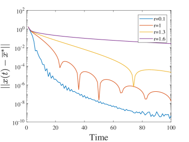
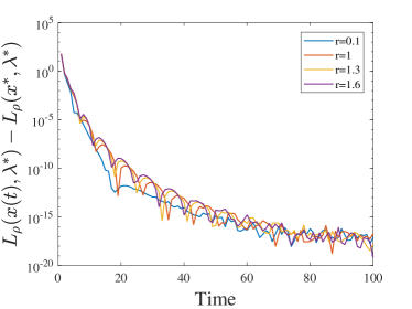
In the first experiment, we take $m=5,$ $n=1$, $e=1$, $\alpha=13$, $\epsilon(t)=\frac{3}{t^{r}}$ and $\rho=1$. Fig. 1 shows the evolution of $\|x(t)-\bar{x}^{*}\|$ and $\mathcal{L}_{\rho}(x(t),\lambda^{*})-\mathcal{L}_{\rho}(x^{*},\lambda^{*})$ for the trajectory $(x(t))_{t\geq t_{0}}$ generated by our dynamical system (3) with different values of $r$, where $0<r<2$.

Refer to caption
Refer to caption
Figure 1: Error analysis with different Tikhonov regularization parameters in the dynamical system (3) for the convex but not strong convex objective function

As shown in Fig. 1, the trajectory (x(t))tt0subscript𝑥𝑡𝑡subscript𝑡0(x(t))_{t\geq t_{0}} converges to the minimizer of minimal norm, and our dynamical system performs better in error x(t)x¯norm𝑥𝑡superscript¯𝑥\|x(t)-\bar{x}^{*}\| when the parameter r𝑟r is small. Further, we can observe that the error ρ(x(t),λ)ρ(x,λ)subscript𝜌𝑥𝑡superscript𝜆subscript𝜌superscript𝑥superscript𝜆\mathcal{L}_{\rho}(x(t),\lambda^{*})-\mathcal{L}_{\rho}(x^{*},\lambda^{*}) is not very sensitive for the Tikhonov regularization parameter.
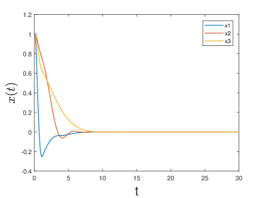
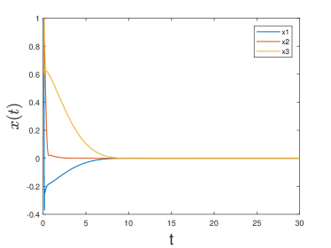
In the second experiment, fix $\alpha=13$, $\rho=1$ and $\epsilon(t)=\frac{3}{t^{r}}$ with $r=0.5$. Then, under different choices of $m$, $n$ and $e$, we illustrate the behaviors of the trajectory $(x(t))_{t\geq t_{0}}$.

Refer to caption
(a) m=5, n=1, e=1.
Refer to caption
(b) m=50, n=10, e=15.
Figure 2: The behaviors of the trajectories $(x(t))_{t\geq t_{0}}$ generated by our dynamical system (3) for the convex but not strong convex objective function

As shown in Fig. 2, the trajectory $(x(t))_{t\geq t_{0}}$ converges to the minimal norm solution $\bar{x}^{*}=(0,0,0)^{T}$ under different choices of $m$, $n$ and $e$.

6.2 The quadratic programming problem

In this subsection, we test the proposed dynamical methods (3) on the linearly constrained quadratic programming problem
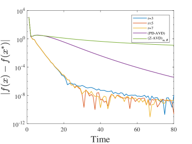
$$\min_{x}f(x)=\frac{1}{2}x^{T}Mx+q^{T}x,\quad\text{ s.t. }Ax=b,$$

where $M\in\mathbb{R}^{n\times n}$ is a symmetric and positive semidefinite matrix, $A\in\mathbb{R}^{m\times n}$, $q\in\mathbb{R}^{n}$, and $b\in\mathbb{R}^{m}$. We compare our dynamical system (3) with $\text{(Z-AVD)}_{\alpha,\theta}$ of [47] and the primal-dual dynamical system with vanishing damping (PD-AVD) of [17]. Here, take starting point $(x(1),\lambda(1),\dot{x}(1))=\mathbf{1}^{(2n+m)\times 1}$, $\epsilon(t)=\frac{1}{t^{r}}$ with $r>2$, $\alpha=15$ and $\rho=1$ in our dynamical system, take starting point $(x(1),\lambda(1),\dot{x}(1),\dot{\lambda}(1))=\mathbf{1}^{2(n+m)\times 1}$ and $\theta=\frac{1}{\alpha-1}$, $\alpha=15$ and $\beta=1$ in (PD-AVD) and take take starting point $(x(1),\lambda(1),\dot{x}(1),\dot{\lambda}(1))=\mathbf{1}^{2(n+m)\times 1}$, $\theta=\frac{1}{2}$ and $\alpha=15$ in $(Z-AVD)_{\alpha,\theta}$. And this numerical experiment uses the ode23 in MATLAB on the interval $[1,100].$

Set $m=20$ and $n=40$. Let $q$ and $b$ be generated by the standard Gaussian distribution and the uniform distribution, respectively. Let $A$ be generated by the standard Gaussian distribution, $M=H^{\top}H$ with $H\in\mathbb{R}^{n\times n}$ generated by the standard Gaussian distribution. By using the Matlab function $quadprog$ with tolerance $10^{-15}$, we get the optimal value $f(x^{*})$. The results are depicted on Fig. 3.

Refer to caption
Refer to caption
Figure 3: Errors of the objective function and the constraint of our dynamical system (3) with different Tikhonov regularization parameters, (PD-AVD) and $(Z-AVD)_{\alpha,\theta}$

As shown in Fig. 3, our dynamical system (3) with a fast vanishing Tikhonov regularization parameter performs better than (PD-AVD) and $\text{(Z-AVD)}_{\alpha,\theta}$ on the quadratic programming problem. In Fig. 3, we also observe that the errors of the objective function and the constraint of our dynamical system are not very sensitive for the fast vanishing Tikhonov regularization parameter.

Conclusion and perspective

In this paper we consider a Tikhonov regularized second-order plus first-order primal-dual dynamical systems with asymptotically vanishing damping. Following the approaches developed in Attouch, Chbani and Riahi [9] and He, Hu and Fang [28], we analyze the convergence properties of the trajectories of the proposed dynamical system (3): For $\alpha\geq 3$, when the Tikhonov regularization parameter tends rapidly to zero, all of the primal-dual gap, the objective function value, and the feasibility measure along the trajectories enjoy the $\mathcal{O}(\frac{1}{t^{2}})$ convergence rate, while when the Tikhonov regularization parameter decreases slowly to zero, the primal trajectory $x(t)$ of the dynamical system converges strongly to the minimal norm solution of the problem (1).

Our study raises some interesting questions:

  • It is interesting to know if the convergence rate of the primal-dual gap and the objective function error along the trajectory of second-order plus first-order primal-dual dynamical system (3) with $\alpha>3$ can be improved to $o(\frac{1}{t^{2}})$, and if the trajectory $x(t)$ converges to a solution of the problem (1) when the Tikhonov regularization parameter tends rapidly to zero.

  • How to discretize the dynamical system (3) to yield an algorithm which enjoys convergence properties matching that of the dynmaical system?

We will consider these questions in the futher work.

Appendix A Some auxiliary results

The following lemmas have been used in the convergence analysis.

Lemma A.1.

[44] Let z𝒳𝑧𝒳z\in\mathcal{X} and let x:[t0,+)𝒳:𝑥subscript𝑡0𝒳x:[t_{0},+\infty)\rightarrow\mathcal{X} be a 𝒞1superscript𝒞1\mathcal{C}^{1} function. If there exists C~>0~𝐶0\widetilde{C}>0 such that

$$\frac{1}{2}\|x(t)-z+\frac{t}{\alpha-1}\dot{x}(t)\|^{2}\leq\widetilde{C},\quad\forall t\geq t_{0},$$

then $(x(t))_{t\geq t_{0}}$ is bounded.

Lemma A.2.

[28, Lemma 6] Assume that g:[t0,+)n:𝑔subscript𝑡0superscript𝑛g:[t_{0},+\infty)\rightarrow\mathbb{R}^{n} is a continuous differentiable function, a:[t0,+)[0,+):𝑎subscript𝑡00a:[t_{0},+\infty)\rightarrow[0,+\infty) is a continuous differentiable function, t0>0subscript𝑡00t_{0}>0, and C0𝐶0C\geq 0. If

$$\|g(t)+\int_{t_{0}}^{t}a(s)g(s)ds\|\leq C,\quad\forall t\geq t_{0},$$

then

$$\sup_{t\geq t_{0}}\|g(t)\|<+\infty.$$

Lemma A.3.

[9, Lemma A.3] Suppose that δ>0𝛿0\delta>0, ϕL1(δ,+)italic-ϕsuperscript𝐿1𝛿\phi\in L^{1}(\delta,+\infty) is a nonnegative and continuous function, and ψ:[δ,+)(0,+):𝜓𝛿0\psi:[\delta,+\infty)\rightarrow(0,+\infty) is a nondecreasing function such that limt+ψ(t)=+subscript𝑡𝜓𝑡\lim_{t\rightarrow+\infty}\psi(t)=+\infty. Then,

$$\lim_{t\rightarrow+\infty}\frac{1}{\psi(t)}\int_{\delta}^{t}\psi(s)\phi(s)ds=0.$$

References

  • [1] C. D. Alecsa and S. C. László, Tikhonov regularization of a perturbed heavy ball system with vanishing damping, SIAM Journal on Optimization, 31 (2021), pp. 2921–2954.
  • [2] F. Alvarez and A. Cabot, Asymptotic selection of viscosity equilibria of semilinear evolution equations by the introduction of a slowly vanishing term, Discrete Contin. Dyn. Syst., 15 (2006), pp. 921–938.
  • [3] H. Attouch, Viscosity solutions of minimization problems, SIAM Journal on Optimization, 6 (1996), pp. 769–806.
  • [4] H. Attouch, A. Balhag, Z. Chbani, and H. Riahi, Damped inertial dynamics with vanishing tikhonov regularization: strong asymptotic convergence towards the minimum norm solution, Journal of Differential Equations, 311 (2022), pp. 29–58.
  • [5] H. Attouch and A. Cabot, Asymptotic stabilization of inertial gradient dynamics with time-dependent viscosity, Journal of Differential Equations, 263 (2017), pp. 5412–5458.
  • [6] H. Attouch, A. Cabot, Z. Chbani, and H. Riahi, Rate of convergence of inertial gradient dynamics with time-dependent viscous damping coefficient, Evolution Equations and Control Theory, 7 (2018), pp. 353–371.
  • [7] H. Attouch, Z. Chbani, J. Fadili, and H. Riahi, Fast convergence of dynamical admm via time scaling of damped inertial dynamics, Journal of Optimization Theory and Applications, 193 (2022), pp. 704–736.
  • [8] H. Attouch, Z. Chbani, P. Juan, and P. Redont, Fast convergence of inertial dynamics and algorithms with asymptotic vanishing viscosity, Mathematical Programming, 168 (2018), pp. 123–175.
  • [9] H. Attouch, Z. Chbani, and H. Riahi, Combining fast inertial dynamics for convex optimization with tikhonov regularization, Journal of Mathematical Analysis and Applications, 457 (2018), pp. 1065–1094.
  • [10] H. Attouch, Z. Chbani, and H. Riahi, Rate of convergence of the nesterov accelerated gradient method in the subcritical case α3𝛼3\alpha\leq 3, ESAIM. Control, Optimisation and Calculus of Variations, 25 (2019).
  • [11] H. Attouch and R. Cominetti, A dynamical approach to convex minimization coupling approximation with the steepest descent method, Journal of Differential Equations, 128 (1996), pp. 519–540.
  • [12] H. Attouch and M. O. Czarnecki, Asymptotic control and stabilization of nonlinear oscillators with non-isolated equilibria, J. Differential Equations, 179 (2002), pp. 278–310.
  • [13] H. Attouch and M. O. Czarnecki, Asymptotic behavior of gradient-like dynamical systems involving inertia and multiscale aspects, J. Differential Equations, 262 (2017), pp. 2745–2770.
  • [14] H. Attouch and S. László, Convex optimization via inertial algorithms with vanishing tikhonov regularization: fast convergence to the minimum norm solution, arXiv:2104.11987, (2021).
  • [15] J. B. Baillon and R. Cominetti, A convergence result for non-autonomous subgradient evolution equations and its application to the steepest descent exponential penalty trajectory in linear programming, J. Funct. Anal., 187 (2001), pp. 263–273.
  • [16] R. I. Bot, E. R. Csetnek, and S. C. László, Tikhonov regularization of a second order dynamical system with hessian driven damping, Mathematical Programming, 189 (2021), pp. 151–186.
  • [17] R. I. Bot and D. K. Nguyen, Improved convergence rates and trajectory convergence for primal-dual dynamical systems with vanishing damping, Journal of Differential Equations, 303 (2021), pp. 369–406.
  • [18] S. Boyd, N. Parikh, E. Chu, B. Peleato, and J. Eckstein, Distributed optimization and statistical learning via the alternating direction method of multipliers, Found. Trends Mach. Learn., 3 (2011), pp. 1–122.
  • [19] A. Cabot, Inertial gradient-like dynamical system controlled by a stabilizing term, Journal of Optimization Theory and Applications, 120 (2004), pp. 275–303.
  • [20] A. Cabot, Proximal point algorithm controlled by a slowly vanishing term: applications to hierarchical minimization, SIAM J. Optim., 15 (2005), pp. 555–572.
  • [21] R. Cominetti, J. Peypouquet, and S. Sorin, Strong asymptotic convergence of evolution equations governed by maximal monotone operators with tikhonov regularization, J. Differential Equations, 245 (2008), pp. 3753–3763.
  • [22] E. R. Csetnek and M. A. Karapetyants, A fast continuous time approach for non-smooth convex optimization with time scaling and tikhonov regularization, arXiv:2207.12023, (2022).
  • [23] M. Fortin and R. Glowinski, Augmented Lagrangian methods, vol. 15, Elsevier, 1983.
  • [24] T. Goldstein, B. O’Donoghue, S. Setzer, and R. Baraniuk, Fast alternating direction optimization methods, SIAM J. Imaging Sci., 7 (2014), pp. 1588–1623.
  • [25] D. R. Han, A survey on some recent developments of alternating direction method of multipliers, Journal of the Operations Research Society of China, 10 (2022), pp. 1–52.
  • [26] A. Haraux, Systèmes dynamiques dissipatifs et applications, Masson, Paris, 1991.
  • [27] X. He, R. Hu, and Y. P. Fang, Convergence rates of inertial primal-dual dynamical methods for separable convex optimization problems, SIAM J. Control Optim., 59 (2021), pp. 3278–3301.
  • [28] X. He, R. Hu, and Y. P. Fang, Fast primal–dual algorithm via dynamical system for a linearly constrained convex optimization problem, Automatica, 146 (2022).
  • [29] X. He, R. Hu, and Y. P. Fang, “second-order primal” + “first-order dual” dynamical systems with time scaling for linear equality constrained convex optimization problems, IEEE Trans. Automat. Control, 67 (2022), pp. 4377–4383.
  • [30] M. Hong and Z. Luo, On the linear convergence of the alternating direction method of multipliers, Mathematical Programming, 162 (2017), pp. 165–199.
  • [31] M. A. Jendoubi and R. May, On an asymptotically autonomous system with tikhonov type regularizing term, Archiv der Mathematik, 95 (2010), pp. 389–399.
  • [32] S. C. László, On the strong convergence of the trajectories of a tikhonov regularized second order dynamical system with asymptotically vanishing damping, Journal of Differential Equations, 362 (2023), pp. 355–381.
  • [33] Z. Lin, H. Li, and C. Fang, Accelerated Optimization for Machine Learning, Springer, Singapore, 2020.
  • [34] H. Luo and L. Chen, From differential equation solvers to accelerated first-order methods for convex optimization, Mathematical Programming, 195 (2022), pp. 735–781.
  • [35] R. Madan and S. Lall, Distributed algorithms for maximum lifetime routing in wireless sensor networks, IEEE Transactions on Wireless Communications, 5 (2006), pp. 2185–2193.
  • [36] Y. Nesterov, A method of solving a convex programming problem with convergence rate 𝒪(1/k2)𝒪1𝑘2\mathcal{O}(1/k2), Sov. Math. Dokl., 27 (1983), pp. 372–376.
  • [37] Y. Nesterov, Gradient methods for minimizing composite functions, Mathematical Programming, 140 (2013), pp. 125–161.
  • [38] B. T. Polyak, Some methods of speeding up the convergence of iteration methods, USSR Comput. Math. Math. Phys., 4 (1964), pp. 1–17.
  • [39] B. Shi, S. S. Du, M. I. Jordan, and W. J. Su, Understanding the acceleration phenomenon via high-resolution differential equations, Mathematical Programming, 195 (2022), pp. 79–148.
  • [40] G. Shi and K. H. Johansson, Randomized optimal consensus of multi-agent systems, Automatica, 48 (2012), pp. 3018–3030.
  • [41] W. Su, S. Boyd, and E. Candès, A differential equation for modeling nesterov’s accelerated gradient method: theory and insights, J. Mach. Learn. Res., 17 (2016), pp. 5312–5354.
  • [42] A. Wibisono, A. C. Wilson, and M. I. Jordan, A variational perspective on accelerated methods in optimization, Proceedings of the National Academy of Sciences, 113 (2016), pp. E7351–E7358.
  • [43] A. C. Wilson, B. Recht, and M. I. Jordan, A lyapunov analysis of accelerated methods in optimization, Journal of Machine Learning Research, 22 (2021), pp. 5040–5073.
  • [44] B. Xu and B. Wen, On the convergence of a class of inertial dynamical systems with tikhonov regularization, Optimization Letters, 15 (2021), pp. 2025–2052.
  • [45] P. Yi, Y. Hong, and F. Liu, Distributed gradient algorithm for constrained optimization with application to load sharing in power systems, Syst. Control Lett., 83 (2015), pp. 45–52.
  • [46] P. Yi, Y. Hong, and F. Liu, Initialization-free distributed algorithms for optimal resource allocation with feasibility constraints and application to economic dispatch of power systems, Automatica, 74 (2016), pp. 259–269.
  • [47] X. Zeng, J. Lei, and J. Chen, Dynamical primal-dual nesterov accelerated method and its application to network optimization, IEEE Transactions on Automatic Control, 68 (2023), pp. 1760–1767.
  • [48] X. Zeng, P. Yi, Y. Hong, and L. Xie, Distributed continuous-time algorithms for nonsmooth extended monotropic optimization problems, SIAM J. Control Optim., 56 (2018), pp. 3973–3993.