Approach to the lower critical dimension of the $\varphi^{4}$ theory in the derivative expansion of the Functional Renormalization Group

Abstract

We revisit the approach to the lower critical dimension $d_{\rm lc}$ in the Ising-like $\varphi^{4}$ theory within the functional renormalization group by studying the lowest approximation levels in the derivative expansion of the effective average action. Our goal is to assess how the latter, which provides a generic approximation scheme valid across dimensions and found to be accurate in $d\geq 2$, is able to capture the long-distance physics associated with the expected proliferation of localized excitations near $d_{\rm lc}$. We show that the convergence of the fixed-point effective potential is nonuniform when $d\to d_{\rm lc}$ with the emergence of a boundary layer around the minimum of the potential. This allows us to make analytical predictions for the value of the lower critical dimension $d_{\rm lc}$ and for the behavior of the critical temperature as $d\to d_{\rm lc}$, which are both found in fair agreement with the known results. This confirms the versatility of the theoretical approach.

I Introduction

Collective behavior characterized by an emergent scale invariance is encountered in a wide variety of physical situations where many degrees of freedom are correlated over long distances. Since its introduction, the Renormalization Group has been the theoretical tool of choice for understanding and describing this phenomenon.wilson-kogut It provides a powerful conceptual framework but, exact results being scarce, the search for generic and efficient approximation schemes has been very active from the very beginning.wilson-wavelet ; wilson-fisher72 ; ma72 ; migdal-kadanoff One relatively recent line of research starts from an exact formulation of the Renormalization Group, in the form of a functional Renormalization Group (FRG) for scale-dependent generating functionals of correlation functions,wegner-houghton ; polchinski ; wetterich93 and introduces potentially nonperturbative approximations through ansatzes for the scale-dependent generating functional under study. The question we want to address is to what extent such generic approximation schemes are able to describe specific problems in which the long-distance behavior involves strongly nonuniform configurations with localized excitations.

An example of such an approximation scheme within the FRG is the so-called derivative expansion of the effective average action (coarse-grained Gibbs free energy in the language of magnetic systems), which amounts to truncating the functional form of the latter in powers of the external momenta or equivalently in gradients of the fields.morris94 The versatility and the effectiveness of the approach have been discussed in several reviews: see Refs. [berges02, ; dupuis21, ]. One key advantage of such an approach is that space dimension $d$ (as well as number of components of the fields, etc.) can be continuously varied at will, allowing one to describe critical behavior from the upper dimension $d_{\rm uc}$ where spatial fluctuations of the local order parameter are easily tamed and classical (mean-field) exponents are observed down to the lower critical dimension $d_{\rm lc}$ below which fluctuations become so strong that no phase transition is possible.

The derivative-expansion approximation focuses on the long-distance properties and, in terms of coarse-grained configurations of the system, works about uniform configurations. One may therefore wonder if such a scheme is able to capture the physics associated with nonuniform configurations containing, e.g., domain walls, spin waves, or localized defects. The answer appears to be positive in the case of configurations involving extended defects, i.e., defects whose energy scales with the system size but in a subextensive way. For instance, the effect of spin waves or domain walls which are associated with the return to convexity of the free energy of an O($N$) model in its low-temperature ordered phase when spatial fluctuations are taken into account,ringwald-wetterich ; tetradis92 ; berges02 ; pelaez-wschebor or the role of singular avalanche events and of scale-free droplet excitations in the critical random-field Ising modeltissier06 ; tissier12 ; tarjus20 are all properly accounted for by the truncated derivative expansion even at the lowest orders.

Yet, the jury is still out when the relevant coarse-grained configurations that control the large-scale behavior involve localized excitations such as the kinks and anti-kinks found in the instanton analysis of the 1-dimensional Ising model.rulquin15 As the approach to the lower critical dimension for systems with a discrete symmetry is expected to be controlled by the proliferation of such localized excitations,bruce81 ; bruce83 ; wallace84 describing the long-distance physics in, say, a model in the Ising universality class such as the $\varphi^{4}$ theory in $d=1+\epsilon$ when $\epsilon\to 0$ is thus a more demanding task for the nonperturbative but approximate FRG than describing the O($N>2$) universality class near $d=2$.footnote_2d

In this paper we investigate how low orders of the derivative expansion in the FRG describe the approach to the lower critical dimension of the $\varphi^{4}$ theory. The lowest order is known as the Local Potential Approximation (LPA)wegner-houghton and is clearly unphysical in low dimensions as it predicts $d_{\rm lc}=2$. Indeed, field renormalization is not accounted for in the LPA, implying that the anomalous dimension of the field is always $\eta=0$. This then misses a crucial ingredient for investigating Ising criticality in dimensions less than $2$. We thus consider the simplest approximation beyond the LPA that incorporates this effect and is often referred to as the LPA’.berges02 ; dupuis21 Working at this level allows us to provide a detailed analytical treatment of the problem.

We stress that the issue per se is not to provide another characterization of the $\varphi^{4}$ theory near $d=1$, as for instance Bruce and Wallacebruce81 ; bruce83 ; wallace84 have already developed an efficient approach in terms a specifically tailored droplet theory. The issue is to assess the ability of a generic nonperturbative approximation scheme within the FRG to quantitatively describe the long-distance physics of a model across the whole range of space dimensions from $d_{\rm lc}$ to $d_{\rm uc}$ without a priori knowledge of the relevant real-space coarse-grained configurations. This also involves the question of the continuity of the critical behavior in the dimensionality of space, which was first investigated by Ballhausen et al.ballhausen04 At odds with the latter work we show that convergence of the critical behavior of the $\varphi^{4}$ theory when $d\to d_{\rm lc}$ within the FRG is nonuniform.

The outline of the paper is as follows. In Sec. II we summarize the FRG framework and the derivative expansion scheme for the scalar $\varphi^{4}$ theory. We also introduce the LPA’ approximation and the approach to the lower critical dimension $d_{\rm lc}$. We then show in Sec. III that the convergence of the fixed-point effective potential to the lower critical dimension is nonuniform in the field and involves a boundary (or interior) layer around the minimum of the potential. We detail the singular perturbation treatment that allows us to find the solution at leading order over the whole range of field. We next present in Sec. IV the results that we obtain for the value the lower critical dimension, which we find close to the exact value $d_{\rm lc}=1$, as well as for the critical temperature and for the critical exponents as $d\to d_{\rm lc}$. We finally give some concluding remarks and provide additional details on the method and the solution in several appendices.

II Functional RG, derivative expansion, and the LPA’

We are interested in the critical behavior of the Ising universality class, which can be represented at a field-theoretical level by a a scalar $\varphi^{4}$ theory,

$$S[\varphi]=\int_{x}\big{(}\frac{1}{2}(\partial_{x}\varphi(x))^{2}+\frac{r}{2}\varphi(x)^{2}+\frac{u}{4!}\varphi(x)^{4}\big{)},$$ (1)

where $\int_{x}\equiv\int d^{d}x$. To do so, we use the FRG approach which is a modern version of Wilson’s RG in which fluctuations are progressively incorporated in the calculation of the partition function of the model through the addition to the action of an infrared (IR) regulator,berges02

$$\Delta S_{k}[\varphi]=\frac{1}{2}\int_{xy}R_{k}(x-y)\varphi(x)\varphi(y),$$ (2)

where $R_{k}$ is an IR cutoff function that suppresses integration of modes with momenta less than $k$ without altering that of modes with momenta larger than $k$. Typical choices of $R_{k}$ will be discussed below. The modified partition function

$$Z_{k}[J]=\int\mathcal{D}\varphi\exp(-S[\varphi]-\Delta S_{k}[\varphi])$$ (3)

is the scale-dependent generating functional of correlation functions and via a modified Legendre transform,

$$\Gamma_{k}[\phi]=-\ln Z_{k}[J]+\int_{x}J(x)\phi(x)-\Delta S_{k}[\phi]),$$ (4)

one can introduce the effective average action $\Gamma_{k}[\phi]$, with $\phi(x)=\langle\varphi(x)\rangle=\delta\ln Z_{k}[J]/\delta J(x)$, which is the scale-dependent generating functional of the 1-particle irreducible (1-PI) correlation functions. It obeys an exact functional RG equation that describes its evolution with the IR scale $k$,wetterich93

$$\partial_{t}\Gamma_{k}[\phi]=\frac{1}{2}\int_{xy}\partial_{t}R_{k}(x-y)\big{[}(\Gamma_{k}^{(2)}[\phi]+R_{k})^{-1}\big{]}_{xy},$$ (5)

where $\Gamma_{k}^{(2)}$ is the second functional derivative of $\Gamma_{k}$ and $t=\ln(k/\Lambda)$ with $\Lambda$ a UV cutoff.

The exact FRG equation in Eq. (5) is a convenient starting point for devising nonperturbative approximation schemes in the form of ansatzes for the functional dependence of the effective average action. One such scheme used to capture the long-distance physics is the derivative expansion in which the Lagrangian associated with $\Gamma_{k}$ is expanded in gradients of the fields,

$$\Gamma_{k}[\phi]=\int_{x}\big{[}U_{k}(\phi(x))+\frac{1}{2}Z_{k}(\phi(x))(\partial_{x}\phi(x))^{2}+{\rm O}(\partial\partial\partial\partial)\big{]}.$$ (6)

When inserted in Eq. (5) the above ansatz provides a hierarchy of coupled FRG equations for the functions $U_{k}(\phi)$, $Z_{k}(\phi)$, etc., where the field configurations involved are now uniform, i.e., $\phi(x)=\phi$.

Scale invariance associated with criticality is described by a fixed point in the FRG equations once the latter have been cast in a dimensionless form via the use of scaling dimensions. One defines dimensionless quantities $\varphi$, $u_{k}$, $z_{k}$, etc., through

$$\phi=k^{D_{\phi}}\varphi,\;\;U_{k}(\phi)=k^{d}u_{k}(\varphi),\;\;Z_{k}(\phi)=Z_{k}z_{k}(\varphi),$$ (7)

etc., where the dimension of the field is related to the anomalous dimension $\eta$ by $D_{\phi}=(d-2+\eta)/2$ and where the field renormalization constant $Z_{k}$ goes as $k^{-\eta}$ in the vicinity of the fixed point. (Note that we have used the same notation $\varphi$ for the bare variable in Eq. (1) and the dimensionless average field, as the former will no longer appear in what follows.)

The hierarchy of FRG equations when expressed in terms of dimensionless quantities takes the form

$$\partial_{t}u_{k}(\varphi)=-du_{k}(\varphi)+\frac{(d-2+\eta_{k})}{2}\varphi u_{k}^{\prime}(\varphi)+\beta_{u}(\varphi;\eta_{k})$$ (8)

$$\partial_{t}z_{k}(\varphi)=\eta_{k}z_{k}(\varphi)+\frac{(d-2+\eta_{k})}{2}\varphi z_{k}^{\prime}(\varphi)+\beta_{z}(\varphi;\eta_{k}),$$

etc., where a prime indicates a derivative with respect to the argument of the function; $\beta_{u}$, $\beta_{z}$, etc. are functionals of $u_{k}^{\prime\prime}$, $z_{k}$, etc., and are given in Appendix A. The fixed points of the flow equations are reached when $t\to-\infty$ (i.e., $k\to 0$) and the left-hand sides go to zero.

As already stressed, a proper description of the approach to the lower critical dimension should incorporate field renormalization and a nonzero anomalous dimension $\eta$. The lowest order of the derivative expansion that achieves this is the so-called LPA’ in which one retains on top of the renormalized potential $U_{k}(\phi)$ a field independent but scale dependent $Z_{k}$. In explicit form, the dimensionless equation for the fixed-point potential is now

$$0=-d\,u(\varphi)+\frac{d-2+\eta}{2}\varphi u^{\prime}(\varphi)+2v_{d}\ell_{0}^{(d)}(u^{\prime\prime}(\varphi);\eta),$$ (9)

where $v_{d}^{-1}=2^{d+1}\pi^{d/2}\Gamma(d/2)$ and $\ell_{0}^{(d)}$ is a (strictly positive) dimensionless threshold function which enforces the decoupling of the low-momentum and high-momentum modes; it is defined in terms of the dimensionless IR cutoff function $r(y=q^{2}/k^{2})=R_{k}(q^{2})/(Z_{k}q^{2})$ by

$$\ell_{0}^{(d)}(w;\eta)=-\frac{1}{2}\int_{0}^{\infty}dyy^{\frac{d}{2}}\frac{\eta r(y)+2yr^{\prime}(y)}{(y[1+r(y)]+w)}$$ (10)

and is described in more detail in Appendix B. We have dropped the subscript $k\to 0$ for quantities at the fixed point in the above equation to simplify the notation.

Deriving Eq. (LABEL:eq_FPpotential) gives an equation for $u^{\prime}(\varphi)$ from which one extracts the equation for its minima $\pm\varphi_{\rm m}$ [through $u^{\prime}(\pm\varphi_{\rm m})=0$],

$$0=\frac{(d-2+\eta)}{2}\varphi_{{\rm m}}+2v_{d}\frac{u^{\prime\prime\prime}(\varphi_{\rm m})}{u^{\prime\prime}(\varphi_{{\rm m}})}\partial_{w}\ell_{0}^{(d)}(w;\eta)|_{w=u^{\prime\prime}(\varphi_{\rm m})},$$ (11)

and deriving one more time gives an equation for the “squared mass” $u^{\prime\prime}(\varphi)$. Both equations will be useful below.

In the LPA’ the field renormalization constant $Z_{k}$ is chosen such that at the minimum of the potential $z_{k}(\pm\varphi{\rm m})=1$.berges02 ; ballhausen04 From Eq. (LABEL:eq_ERGEdimensionless) and the explicit form of $\beta_{z}$ given in Appendix A one then obtains that

$$\eta=\frac{4v_{d}}{d}u^{\prime\prime\prime}(\varphi_{\rm m})^{2}m_{4,0}^{(d)}(u^{\prime\prime}(\varphi_{\rm m});\eta),$$ (12)

where $m_{4,0}^{(d)}$ is another (strictly positive) dimensionless threshold function defined by

$$m_{4,0}^{(d)}(w;\eta)=\frac{1}{2}\int_{0}^{\infty}dyy^{\frac{d}{2}}\frac{1+(yr(y))^{\prime}}{(y[1+r(y)]+w)^{4}}\bigg{[}2\eta(yr(y))^{\prime}$$ (13)

$$+4(y^{2}r^{\prime}(y))^{\prime}-4\,\frac{y[1+(yr(y))^{\prime}][\eta r(y)+2yr^{\prime}(y)]}{y[1+r(y)]+w}\bigg{]}$$

and discussed in Appendix B. Once a specific form for the dimensionless IR cutoff function $r(y)$ has been chosen, the solution of Eqs. (LABEL:eq_FPpotential-LABEL:eq_threshold_m40) fully characterizes the LPA’ fixed point. In what follows we will use two much studied forms of $r(y)$:

$$r(y)=\alpha\Theta(1-y)(1-y)/y$$ (14)

$$r(y)=\alpha e^{-y}/y$$

where $\Theta$ is the Heaviside step function and $\alpha$ is a variational parameter of O(1) that can be determined, e.g., by the principle of minimum sensitivity.litim01 ; dupuis21 ; balog19 We will refer to these two choices as Theta and Exponential cutoff functions.

We illustrate the results for the fixed point at LPA’ and the choice of the Theta cutoff function with $\alpha=1$ (similar results are obtained with other choices, see the discussion further below) in Figs. 1 and 2. Fig 1 displays the evolution of the dimensionless potential $u(\varphi)$ and the “square mass” function $u^{\prime\prime}(\varphi)$ as the space dimension $d$ decreases, and Fig. 2 that of the field scaling dimension $D_{\phi}=(d-2+\eta)/2$. To show that a similar behavior in low dimension is also expected for higher orders of the derivative expansion, so that the LPA’ level is not atypical, we plot the evolution with $d$ of the dimensionless potential and of the field dimension $D_{\phi}$ at the second order of the derivative expansion for which the field renormalization is now a full function of the field [see Eq. (LABEL:eq_ERGEdimensionless)] in Fig. 3

Figure 1: Dimensionless effective potential $u(\varphi)$ (a) and its second derivative $u^{\prime\prime}(\varphi)$ (b) at the LPA’ fixed point for several dimensions $d$ between $1.6$ and $1.1$. We have used the Theta IR cutoff function with $\alpha=1$ and a numerical resolution of the FRG equations.

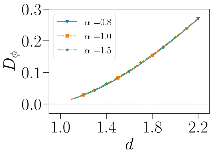
Figure 2: Variation with the space dimension $d$ of the field scaling dimension $D_{\phi}=(d-2+\eta)/2$ at the LPA’ fixed point as obtained from a numerical resolution and the Exponential IR cutoff function.

Figure 3: Dimensionless effective potential $u(\varphi)$ (a) and field scaling dimension $D_{\phi}=(d-2+\eta)/2$ (b) at the fixed point obtained of the second order of the derivative expansion for several dimensions $d$ between $1.8$ and $1.11$. We have used the Exponential IR cutoff function with $\alpha=1$ and a numerical resolution of the FRG equations.

A defining property of the lower critical dimension is that $(d-2+\eta)|_{d\to d_{l}}\to 0$. This is equivalent to stating that the scaling dimension $D_{\phi}$ of the field vanishes (see above and Fig. 2). If the field does not rescale, its fluctuations along the RG flow remain of order $1$ in terms of the dimensionful field and ordering associated with a nonzero dimensionful average field in zero applied source is impossible. We thus find it convenient to define

$$\tilde{\epsilon}(d)=\frac{d-2+\eta}{2(2-\eta)},$$ (15)

which goes to $0$ as $d\to d_{\rm lc}$. We use the notation $\tilde{\epsilon}$ to avoid confusion with $\epsilon=d-d_{\rm lc}$ (with $d_{\rm lc}=1$ in an exact treatment.)

Another anticipated feature of the approach to the lower critical dimension is the fact that the propagator of the theory approaches a pole. Indeed, the lower critical dimension corresponds to the merging of the critical fixed point and the zero-temperature fixed point associated with the symmetry-broken ordered phase, and the return to convexity of the effective potential along the FRG flow is controlled in the latter by the presence of a pole in the propagator.tetradis92 ; berges02 ; pelaez-wschebor In the LPA’ the dimensionless propagator is given by

$$p(y;\varphi)=\frac{1}{y[1+r(y)]+u^{\prime\prime}(\varphi)}$$ (16)

and must of course be positive. With the choice of the Theta cutoff function in Eq. (LABEL:eq_cutoff_choices) the pole in either in $y=q^{2}/k^{2}=0$ and $u^{\prime\prime}(\varphi)=-\alpha$ when $\alpha<1$ or in $y=1$ and $u^{\prime\prime}(\varphi)=-1$ when $\alpha>1$. With the Exponential cutoff function the pole is either in $y=0$ and $u^{\prime\prime}(\varphi)=-\alpha$ when $\alpha<1$ or in $y=\ln\alpha$ and $u^{\prime\prime}(\varphi)=-(1+\ln\alpha)$ when $\alpha>1$: see Appendix B.

In the following we will investigate in more detail the structure of the fixed-point solution at LPA’ when $d\to d_{\rm lc}$. As the numerical solution becomes harder if not impossible in this limit, progress should be made through an analytical treatment. We stress again that contrary to what happens for the O($N>2$) models where there are Goldstone modes associated with the breaking of a continuous symmetry which quite straightforwardly imply that $d_{\rm lc}=2$,zinn-justin89 ; berges02 ; delamotte04 ; dupuis21 the LPA’ or any level of truncation of the derivative expansion within the FRG need not predict the exact value of the lower critical dimension, $d_{\rm lc}=1$, for the present model with a discrete $Z_{2}$ symmetry. The approximate $d_{\rm lc}$ must then be computed.

III Nonuniform convergence to the lower critical dimension

III.1 nonuniform convergence and boundary layer

Consider the LPA’ fixed-point equation for the second derivative of the potential,

$$0=-u^{\prime\prime}(\varphi)+\tilde{\epsilon}(d)\varphi u^{\prime\prime\prime}(\varphi)+\frac{2v_{d}}{2-\eta(d)}\partial^{2}_{\varphi}\ell_{0}^{(d)}(u^{\prime\prime}(\varphi);\eta(d)),$$ (17)

where $\eta=2-d+d\tilde{\epsilon}+{\rm O}(\tilde{\epsilon}^{2})$. As the dependence of $\tilde{\epsilon}$ on $d$ is expected to be monotonic, one can study the above equation at fixed $\tilde{\epsilon}$ instead of fixed $d$, and when $\tilde{\epsilon}\to 0$,

$$0=-u^{\prime\prime}(\varphi)+\tilde{\epsilon}\varphi u^{\prime\prime\prime}(\varphi)+\frac{2v_{d}}{d}\partial^{2}_{\varphi}\ell_{0}^{(d)}(u^{\prime\prime}(\varphi);2-d),$$ (18)

where $d\equiv d(\tilde{\epsilon})\to d_{\rm lc}$ and $d_{\rm lc}$ a priori unknown.

If $u^{\prime\prime}(\varphi)$, its first derivatives, and $\varphi$ are of O(1) the second term in Eq. (18) can be set to zero as a leading approximation in which $\tilde{\epsilon}=0$ altogether. This describes a uniform convergence toward the lower critical dimension, as was assumed in Ref. [ballhausen04, ]. Our claim, which we substantiate below, is that the second term leads to a singular-perturbation problem and that the limit $\tilde{\epsilon}\to 0$ is nonuniform in the field.

From the shape of the fixed-point potential in Fig. 1 one can see that three domains of field values can be distinguished: the large-field region, $|\varphi|\to+\infty$, where $u(\varphi)$ and its first derivatives blow up, the region of the minima where the first derivative is zero but higher-order derivatives grow large as $d$ decreases, and the inner region of fields of order O(1) in which the potential and its derivatives appear of O(1). The latter region should be describable by the $\tilde{\epsilon}=0$ equation (plus regular perturbation in $\tilde{\epsilon}$) and the large-field one corresponds to the situation where the square mass $u^{\prime\prime}(\varphi)$ diverges and the nontrivial beta functions go to zero to only leave the scaling part of the equation: here, $0=-u^{\prime\prime}(\varphi)+\tilde{\epsilon}\varphi u^{\prime\prime\prime}(\varphi)$, which leads to

$$u^{\prime\prime}(\varphi)\sim|\varphi|^{\frac{1}{\tilde{\epsilon}}}\;\;{\rm when}\;\;\varphi\to\pm\infty.$$ (19)

The region of the close vicinity of the minima needs more care and entails a boundary-layer treatment. (Note that interior layer would be more adequate in this case than boundary layer because the region in which variation is very fast is away from the boundaries, but with this caveat we will nonetheless keep using the term boundary layer.) A unique global solution valid for all fields is finally obtained by “matching” the partial solutions obtained in each domain in the intermediate regions of field over which they overlap. This matching procedure is a key element of the singular perturbation treatment.singular-perturbation

The potential $u(\varphi)$ being $Z_{2}$ symmetric, we choose to restrict our analysis to positive fields, $\varphi\geq 0$.

III.2 The solution of the $\tilde{\epsilon}=0$ equation

Consider first the LPA’ equation for $\tilde{\epsilon}=0$. Introducing for simplicity the notation $w(\varphi):=u^{\prime\prime}(\varphi)$, one has

$$w(\varphi)=\frac{2v_{d}}{d}\partial^{2}_{\varphi}\ell_{0}^{(d)}(w(\varphi);2-d),$$ (20)

where $d=d_{\rm lc}$, which we assume in the following to be strictly less than $2$, and the initial conditions are $w(0)=w_{0}$ and all the odd derivatives of $w$ are zero in $\varphi=0$. Let also define $\Phi(\varphi):=\ell_{0}^{(d)}(w(\varphi);2-d)$. The function $\ell_{0}^{(d)}(w;2-d)$ being monotonically increasing with $w$, one can invert it and define $w=F(\Phi)$ with $F$ such that $F(\ell_{0}^{(d)}(w;2-d)=w$. Eq. (20) can then be rewritten as

$$\partial^{2}_{\varphi}\Phi(\varphi)=\frac{d}{2v_{d}}F(\Phi(\varphi)),$$ (21)

which is the equation of motion of an anharmonic oscillator $\Phi(\varphi)$ with $\varphi$ playing the role of time and $(d/(2v_{d}))F(\Phi)$ being the force. The solution for $\Phi(\varphi)$ is a periodic function starting in $\Phi_{0}=\ell_{0}^{(d)}(w_{0};2-d)$ with a velocity $\partial_{\varphi}\Phi|_{0}=0$. The half-period $\varphi_{*}$ corresponds to the first time at which the velocity is again equal to $0$. By using the energy balance equation associated with Eq. (21),

$$\int_{\Phi_{0}}^{\Phi(\varphi)}d\Phi^{\prime}\frac{d}{2v_{d}}F(\Phi^{\prime})=\frac{1}{2}[\partial_{\varphi}\Phi(\varphi)]^{2},$$ (22)

one derives that $\varphi_{*}$ is obtained from

$$\int_{0}^{\varphi_{*}}d\varphi^{\prime}\partial_{\varphi^{\prime}}\Phi(\varphi^{\prime})w(\varphi^{\prime})=0.$$ (23)

Note that $\varphi_{*}$ and the solution $\Phi(\varphi)$ are parametrized by the initial value $w_{0}$.

Because of the monotonic relation between $\Phi$ and $w$, the solution for $w(\varphi)$ is also a periodic function of half-period $\varphi_{*}$ that oscillates between a minimum value $w_{0}$ and a maximum one $w_{*}=w(\varphi_{*})$, the two values being uniquely related. Clearly, this solution cannot be that of the full problem (which is not periodic: see Fig. 1(b)) when $\varphi$ is close to and larger than $\varphi_{*}$. As alluded to above, a boundary-layer type of solution must replace the solution of the $\tilde{\epsilon}=0$ equation. Since $w(\varphi)$ is very large in the close vicinity of the (exact) minimum of the potential, $\varphi_{\rm m}$, a potential matching between the two types of solution must take place for $\varphi<\varphi_{\rm m}\lesssim\varphi_{*}$, which requires that $w(\varphi_{*})$ very large. In this limit, it can be shown from the properties of the $\tilde{\epsilon}=0$ solution (see Appendix C) that

$$\varphi_{*}\sim\sqrt{\ln w_{*}}.$$ (24)

The matching requirement and the constraint it puts on the value of $w(\varphi_{0})=w_{0}$ will be considered in more detail below.

III.3 The inner solution within the layer

The $\tilde{\epsilon}=0$ equation ceases to be the proper description when the second term of Eq. (18) becomes of the same order as the other terms and a new solution must be found. Guided by the numerical solution and by physical intuition, we argue that a new solution takes place within a “boundary layer” (actually, an “interior layer”: see the above comment) around the minimum $\varphi_{\rm m}$ of the potential. In this region, $w\gg 1$, and Eq. (18) becomes

$$0=-w(\varphi)+\tilde{\epsilon}\varphi w^{\prime}(\varphi)+\frac{2v_{d}}{d}\alpha A_{d}\partial^{2}_{\varphi}\left[\frac{1}{w(\varphi)}\right],$$ (25)

where we have used that for large square mass $w$, Eq. (10) gives

$$\ell_{0}^{(d)}(w;2-d)\sim\frac{\alpha A_{d}}{w}+{\rm O}(\frac{1}{w^{2}})$$ (26)

with, after some manipulations, $A_{d}$ obtained as

$$A_{d}=d\int_{0}^{\infty}dyy^{\frac{d}{2}}\left[\frac{r(y)}{\alpha}\right].$$ (27)

More details are given in Appendix B. It is then convenient to rescale the field $\varphi$ by a multiplicative factor $\sqrt{d/(2\alpha v_{d}A_{d})}$, so that Eq. (25) reads

$$0=-w(\varphi)+\tilde{\epsilon}\varphi w^{\prime}(\varphi)+\partial^{2}_{\varphi}\left[\frac{1}{w(\varphi)}\right],$$ (28)

with no explicit dependence on $d$ (which we recall should be taken as $d_{\rm lc}$ in the limit $\tilde{\epsilon}\to 0$ that we consider).

In the vicinity of $\varphi_{\rm m}$ we introduce a rescaled variable $x=(\varphi-\varphi_{\rm m})/\delta(\tilde{\epsilon})$ with $x={\rm O}(1)$ as $\tilde{\epsilon}\to 0$. By balancing the first two terms of Eq. (28) one obtains that $\delta(\tilde{\epsilon})=\tilde{\epsilon}\varphi_{\rm m}$, i.e.,

$$x=\frac{\varphi-\varphi_{\rm m}}{\tilde{\epsilon}\varphi_{\rm m}},$$ (29)

where we assume for now, and check later on, that $\tilde{\epsilon}\varphi_{\rm m}\to 0$ when $\tilde{\epsilon}\to 0$. By also requiring that the third term is of the same order of magnitude as the first two, one is further led to introduce a function $g(x)$ which is defined by

$$w(\varphi)=\frac{g(x)}{\tilde{\epsilon}\varphi_{\rm m}}$$ (30)

and which is of O(1) when $x$ is of O(1). The LPA’ equation in the boundary layer can then be expressed as

$$-g(x)+g^{\prime}(x)+\partial^{2}_{x}\left[\frac{1}{g(x)}\right]=0.$$ (31)

This is complemented by the equation for the minimum, Eq. (11), which leads to

$$g^{\prime}(0)=g(0)^{3}.$$ (32)

The boundary layer equation can be solved in an implicit form by first introducing the auxiliary function

$$X(x)=g(x)+\partial_{x}\left[\frac{1}{g(x)}\right]$$ (33)

which satisfies $X(0)=0$ because of Eq. (32). Then, one has that

$$g(x)=X^{\prime}(x),$$ (34)

and the solution for $g(x)$ as a function of $X(x)$ is given by

$$g(x)=g(0)\frac{e^{-\frac{X(x)^{2}}{2}}}{\left[1-\sqrt{\frac{\pi}{2}}g(0)+g(0)\int_{X(x)}^{+\infty}dt\,e^{-\frac{t^{2}}{2}}\right]}\,.$$ (35)

The interest of the above expression is that it allows us to study the limit $x\to+\infty$ and require matching with the outer solution at large field, $w(\varphi\to\infty)\sim\varphi^{1/\tilde{\epsilon}}\to+\infty$, already derived. (This is the standard method of matched asymptotic expansions used in singular perturbation problems.) Choosing the matching region such that $1/\tilde{\epsilon}\gg x\gg 1$, the latter then imposes that $g(x)$ diverges as $\exp(x)$ at large positive $x$. From Eqs. (35) and (33) it is straightforward to see that one must have

$$1-\sqrt{\frac{\pi}{2}}g(0)=0,$$ (36)

which fixes $g(0)$ and via Eq. (32) $g^{\prime}(0)$.

We plot in Fig. 4 the inverse of $g(x)$, as obtained from the solution of the above equations. It is a monotonically decreasing function. When $x$ is negative and $|x|$ very large, it behaves as one finds that

$$\frac{1}{g(x)}\sim\sqrt{2}|x|\sqrt{\ln|x|}\Big{[}1+{\rm O}\left(\frac{\ln(\ln|x|)}{\ln|x|}\right)\Big{]},$$ (37)

an expression which will be useful when considering matching with the outer solution obtained from the equation with $\tilde{\epsilon}=0$ (see Sec. III.2).

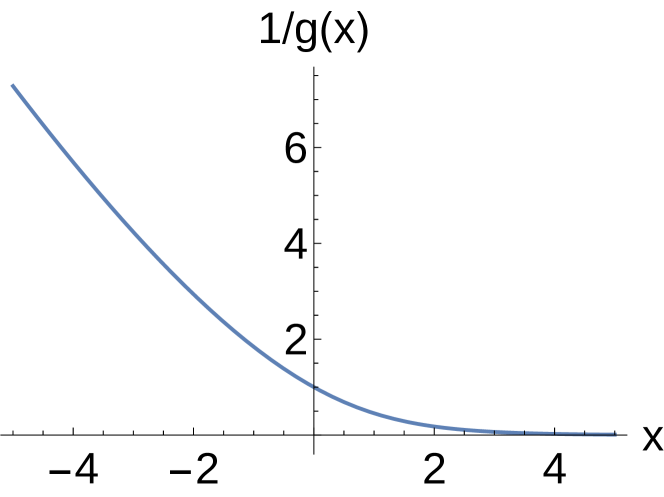
Figure 4: Inverse of the inner solution $g(x)$ giving the square-mass function within the layer around the minimum of the potential. The latter corresponds to $x=0$.

III.4 Matching the inner solution with that of the $\tilde{\epsilon}=0$ equation

At least at the present LPA’ level of approximation the solution $g(x)$ within the layer around $\varphi_{\rm m}$ is fully determined by matching with the outer solution obtained at large field. However, the relation between $\varphi_{\rm m}$ and $\tilde{\epsilon}$ is yet to be determined. It is also crucial to check that matching with the outer solution corresponding to fields less than $\varphi_{\rm m}$ and to the $\tilde{\epsilon}=0$ equation can be enforced, so that a solution can be constructed for all field values.

In Sec. III.2 we have argued that matching should take place for fields $\varphi<\varphi_{\rm m}\lesssim\varphi_{*}$, where furthermore the outer solution associated with the $\tilde{\epsilon}=0$ equation should be such that $1\ll w(\varphi)\ll w(\varphi_{\rm m}),w_{*}$. We can choose the matching region where the two solutions overlap such that

$$\varphi_{\rm m}-\varphi={\rm O}((\tilde{\epsilon}\varphi_{\rm m})^{a})\;\;{\rm with}\;0<a<1,$$ (38)

and, as a result, $x\sim-(\tilde{\epsilon}\varphi_{\rm m})^{1-a}$ is negative and very large. The asymptotic limit of the inner solution is then given by Eq. (37), which implies that

$$w_{*}\gg w(\varphi)={\rm O}\big{(}\tilde{\epsilon}\varphi_{\rm m})^{-a}|\ln(\tilde{\epsilon}\varphi_{\rm m})|^{-\frac{1}{2}}\big{)}\to+\infty.$$ (39)

From Eq. (23) one can obtain the relation between $w_{*}$ and $w_{0}$ as

$$0 =\int_{w_{0}}^{w_{*}}dw^{\prime}w^{\prime}\partial_{w^{\prime}}\Phi(w^{\prime})$$ (40)

$$=w_{*}\Phi(w_{*})-w_{0}\Phi(w_{0})-\int_{w_{0}}^{w_{*}}dw^{\prime}\Phi(w^{\prime}),$$

where, we recall, $\Phi(w)=\ell_{0}^{(d)}(w;2-d)$ with the latter given in Eq. (10). To evaluate the quantities in the above equation we split the integral by introducing an intermediate value $w_{c}$, which we choose positive and of O(1). Taking into account that $w_{*}$ diverges and using the property that the function $\Phi(w)$ is monotonically decreasing and asymptotically goes to zero as $\alpha A_{d}/w+{\rm O}(1/w^{2})$, we transform Eq. (40) into

$$\alpha A_{d}\ln w_{*}=-w_{0}\Phi(w_{0})+\int_{w_{0}}^{w_{c}}dw^{\prime}\Phi(w^{\prime}),$$ (41)

up to O(1) terms, and, since $w_{0}$ and $w_{c}$ are of O(1), this implies that $\Phi(w_{0})$ diverges. This can only occur if $w_{0}$ approaches the pole of the propagator, which we call $w_{P}$ and can be either $-1$, $-\alpha$, or $-(1+\ln\alpha)$ depending on the IR cutoff function and on $\alpha$ [see Eq. 16) and below]. Notwithstanding the precise asymptotic behavior of $\Phi(w)\equiv\ell_{0}^{(d)}(w;2-d)$ when the pole is approached (this depends on the IR cutoff function, see Appendix B), the second term of the right-hand side is subdominant compared to the first one and one has

$$\Phi(w_{0})\sim\frac{\alpha A_{d}}{|w_{P}|}\ln w_{*}\to+\infty.$$ (42)

Matching thus entails that the square mass in zero field $w_{0}\to w_{P}^{+}$, which, as argued above, is one of the expected hallmarks of the approach to the lower critical dimension. Note that in the limit process $w_{0}$ must remain strictly larger than the pole $w_{P}$ by a quantity that goes to zero with $\tilde{\epsilon}$: this again illustrates the highly singular and nonuniform approach to the lower critical dimension.

To complete the proof, we note that in the chosen matching region, the leading behavior of $w(\varphi)$ in the boundary layer and that corresponding to the $\tilde{\epsilon}=0$ solution obey the same equation, $-w(\varphi)+\partial^{2}_{\varphi}[1/w(\varphi)]=0$. The difference is in the boundary condition at large field: The $\tilde{\epsilon}=0$ is limited by $\varphi_{*}$ while it is convenient to consider the boundary-layer one up to $\varphi_{\rm m}$. Taking this into account, the solution can then be obtained either as

$$\varphi_{\rm m}-\varphi(w)=\tilde{\epsilon}\varphi_{\rm m}|x|\approx\frac{\sqrt{2}}{2}\frac{1}{w\sqrt{\ln(\frac{1}{\tilde{\epsilon}\varphi_{\rm m}w})}}$$ (43)

or as

$$\varphi_{*}-\varphi(w)\approx\frac{\sqrt{2}}{2}\frac{1}{w\sqrt{\ln(\frac{w_{*}}{w})}}.$$ (44)

Matching between the two solutions is then enforced at leading order if

$$\varphi_{*}\sim\varphi_{\rm m},$$ (45)

$$w_{*}\sim\frac{1}{\tilde{\epsilon}\varphi_{\rm m}}\sim w_{\rm m},$$

which, since $\varphi_{*}$ diverges as $\sqrt{\ln w_{*}}$ (see Eq. (24) and Appendix C), immediately leads to

$$w_{\rm m}\sim w_{*}\sim\frac{1}{\tilde{\epsilon}\sqrt{\ln(\frac{1}{\tilde{\epsilon}})}},$$ (46)

$$\varphi_{\rm m}\sim\varphi_{*}\sim\sqrt{\ln(\frac{1}{\tilde{\epsilon}})}+{\rm O}(\ln\ln(\frac{1}{\tilde{\epsilon}})).$$

So, as anticipated the location of the minimum of the potential $\varphi_{\rm m}$ diverges when $\tilde{\epsilon}\to 0$ but the width of the layer $\tilde{\epsilon}\varphi_{\rm m}$ goes to $0$. This is supported by the numerical resolution of the LPA’ flow equation for values of $d$ approaching as close as possible the lower critical dimension: see Fig. 5. This result is different than the prediction of the previous FRG analysis of the approach to the lower critical dimension within the truncated derivative expansion in Ref. [ballhausen04, ]. The latter missed the emergence of the boundary layer near the minimum of the potential, which led to the scaling $\varphi_{\rm m}\sim 1/\sqrt{\tilde{\epsilon}}$ that does not fit the data as shown in Fig. 5a.

Figure 5: (a) Location of the minimum of the potential $\varphi_{\rm m}$ divided by $\sqrt{\ln(1/\tilde{\epsilon})}$ as a function of $\tilde{\epsilon}$. (b) Same but for the square mass $w_{\rm m}\equiv u^{\prime\prime}(\varphi_{\rm m})$ multiplied by $\delta(\tilde{\epsilon})=\tilde{\epsilon}\sqrt{\ln(1/\tilde{\epsilon})}$. As predicted, both curves appear to essentially go to finite nonzero values as $\tilde{\epsilon}\to 0$, in agreement with our singular perturbation analysis (loglog corrections are not detectable with our data). On the other hand the prediction from [ballhausen04, ] (dashed black line in (a)) clearly does not fit the data. The data points in (a) and (b) are obtained from the numerical resolution of the LPA’ fixed-point equations for the Exponential cutoff functions with several different values of the prefactor $\alpha$.

Collecting all of the above results allows one to build a fixed-point solution $w(\varphi)\equiv u^{\prime\prime}(\varphi)$ that is valid over the whole range of field values when $\tilde{\epsilon}\to 0$. One can note the peculiar form of the present singular perturbation problem in which neither the initial condition in $\varphi=0$ nor the location of the layer in $\varphi_{\rm m}$ are determined a priori and must be determined through the matching procedure.

We now discuss the consequences for the LPA’ prediction of the lower critical dimension $d_{\rm lc}$, the behavior of the critical temperature $T_{c}$, and the critical exponents as $\tilde{\epsilon}\to 0$.

IV Results

IV.1 Determination of the lower critical dimension

To determine the value of the lower critical dimension $d_{\rm lc}$ we consider the last of the LPA’ equations that we have not yet used, i.e., Eq. (12) for the anomalous dimension of the field. This equation involves the square mass $w(\varphi)$ in the boundary layer only. When $\tilde{\epsilon}\to 0$, $w(\varphi_{\rm m})\to\infty$, $\eta\to 2-d$, and the threshold function $m_{4,0}^{(d)}(w;\eta)$ can be replaced in Eq. (12) by its asymptotic form,

$$m_{4,0}^{(d)}(w;2-d)\sim\frac{\alpha dA_{d}-\alpha^{2}B_{d}}{w^{4}}$$ (47)

where $A_{d}$ is given in Eq. (27) and, as derived in Appendix B,

$$B_{d}=\frac{3d-2}{2}\int_{0}^{\infty}dyy^{\frac{d}{2}}[(y\frac{r(y)}{\alpha})^{\prime}]^{2}\,.$$ (48)

As before a prime indicates a derivative with respect to the argument of the function and the IR cutoff functions that we use are defined in Eq. (LABEL:eq_cutoff_choices).

With the rescaling of the field and the notations introduced in Sec. III.3, one can then rewrite Eq. (12) as

$$2-d=2(d-\alpha\,\frac{B_{d}}{A_{d}})\frac{g^{\prime}(0)^{2}}{g(0)^{4}}=\frac{4}{\pi}(d-\alpha\,\frac{B_{d}}{A_{d}})$$ (49)

where we have used that the solution within the layer around the minimum satisfies Eqs. (32) and (36). The solution of the above equation gives $d=d_{\rm lc}$.

For the Theta cutoff function, $B_{d}/A_{d}=(3d-2)/4$ (see Appendix B), so that we obtain an explicit analytical expression for the lower critical dimension:

$$d_{\rm lc}(\alpha)=2\frac{\pi-\alpha}{\pi+4-3\alpha},$$ (50)

which for instance predicts $d_{\rm lc}=1.03419\cdots$ for $\alpha=1$. Note that the solution derived in the previous section required $d<2$. This entails that $\alpha<2$, so that the pole in $\alpha=(\pi+4)/3$ is not attained. The variation of $d_{\rm lc}$ with $\alpha$ is shown in Fig. 6.

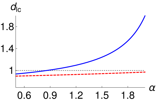
Figure 6: Lower critical dimension $d_{\rm lc}(\alpha)$ predicted by the solution of the LPA’ with the Theta (upper blue curve) and Exponential (lower red curve) IR cutoff functions.

For the Exponential cutoff function, one finds that $B_{d}/A_{d}=2^{-(1+d/2)}(3d-2)/4$ (see Appendix B), so that $d_{\rm lc}$ is solution of the implicit equation

$$d_{\rm lc}(\alpha)=2\frac{\pi-\alpha_{*}(d)}{\pi+4-3\alpha_{*}(d)}$$ (51)

with $\alpha_{*}(d)=2^{-(1+d/2)}\alpha$. The outcome is plotted in Fig. 6.

We therefore obtain that for a reasonable range of the variational parameter $\alpha$ (which cannot be fixed by any principle of minimum sensitivity on the variation of $d_{\rm lc}(\alpha)$ because the latter does not display a minimum at the present level of approximation) the predicted lower critical dimension is indeed close to the exact result, $d_{\rm lc}=1$ (within $10\%$ for the Exponential cutoff function; the result found with the Theta regulator appears less well-behaved than that of the Exponential cutoff).

IV.2 Critical temperature $T_{c}$ as $\tilde{\epsilon}\to 0$

One of the many defining properties of the lower critical dimension is that the critical temperature $T_{c}$ goes to zero. This is a bare quantity which is not easily retrieved from the RG flow. However when it goes to zero, a simple reasoning based on the Boltzmann form of the distribution suggests that the field scales as the square root of the inverse temperature. As the dimension of the field at criticality goes to zero at the lower critical dimension, one therefore expects that $T_{c}\sim 1/\varphi_{\rm m}^{2}$. This is indeed what is found in the correspondance between the Wilsonian dimensionless action of the O($N>2$) model and the nonlinear sigma model near the lower critical dimension $d=2$.??? Together with Eq. (LABEL:eq_matchingfinal), this scaling leads to

$$T_{c}\sim\frac{1}{\ln(\frac{1}{\tilde{\epsilon}})}\to 0$$ (52)

when $\tilde{\epsilon}\to 0$.

Recast in terms of the field dimension $D_{\phi}=(d-2+\eta)/2$ the above expression is equivalent to

$$T_{c}\propto\frac{1}{\ln(\frac{1}{D_{\phi}})}.$$ (53)

This relation is similar to that obtained by Bruce and Wallace from a detailed droplet theory.bruce81 ; bruce83 In the latter, the expansion is performed in $\epsilon=d-d_{\rm lc}$ with $d_{\rm lc}=1$. The outcome is that $T_{c}$ has a simple expansion in powers of $\epsilon$, $T_{c}\propto\epsilon+{\rm O}(\epsilon^{2})$, but $D_{\phi}$ has instead a singular behavior, with $D_{\phi}\sim e^{-2/\epsilon}/\epsilon$. Combining the two gives Eq. (53). Note that this relation is not verified by the prediction of Ref. [ballhausen04, ].

IV.3 Stability of the fixed point, essential scaling, and correlation-length critical exponent as $\tilde{\epsilon}\to 0$

The stability of the fixed point can be studied by looking at perturbations around it and the resulting eigenvalue equation equation obtained in linear order of the perturbation. For the present LPA’ approximation, after introducing small perturbations around the fixed point as $w_{k}(\varphi)=w(\varphi)+k^{\lambda}\delta w(\varphi)$, $\eta_{k}=\eta+k^{\lambda}\delta\eta$, $\varphi_{\rm mk}=\varphi_{\rm m}+k^{\lambda}\delta\varphi_{\rm m}$, etc., with $\lambda$ an eigenvalue to be determined, the linearized equation for $\delta w(\varphi)$ reads

$$\lambda\delta w(\varphi)=-(2-\eta)\delta w(\varphi)+(2-\eta)\tilde{\epsilon}\varphi\delta w^{\prime}(\varphi)+$$ (54)

$$2v_{d}\partial^{2}_{\varphi}[\partial_{w}\ell_{0}^{(d)}(w(\varphi);\eta)\delta w(\varphi)]+\big{(}w(\varphi)+\frac{1}{2}\varphi w^{\prime}(\varphi)$$

$$+2v_{d}\partial^{2}_{\varphi}[\partial_{\eta}\ell_{0}^{(d)}(w(\varphi);\eta)]\big{)}\delta\eta,$$

and the expressions for $\delta\eta$ and $\delta\varphi_{\rm m}$ are given in Appendix D. We are especially interested in finding the relevant eigenvalue that gives the correlation length exponent $\nu$ which is known to diverge at the lower critical dimension in an exact treatment.

As we did for the fixed point, one can attempt a singular perturbation analysis when $\tilde{\epsilon}\to 0$ (and $\eta\to 2-d$) by looking separately at the $\tilde{\epsilon}=0$ equation for $\varphi$ of O(1) and at an equation in terms of the scaled variable $x=(\varphi-\varphi_{\rm m})/(\tilde{\epsilon}\varphi_{\rm m})$ near the minimum $\varphi_{\rm m}$. However, one immediately sees that if $\lambda={\rm O}(\tilde{\epsilon})$ or more generally goes to zero when $\tilde{\epsilon}\to 0$, which is the expected behavior of the relevant eigenvalue(s), working at the leading order in $\tilde{\epsilon}$ does not allow the determination of $\lambda$ beyond the fact that it starts as $0$.

This can be illustrated by considering one eigenvalue that can be exactly obtained together with its eigenfunction. One easily finds that $\lambda=-(2-\eta)\tilde{\epsilon}$ is a solution of Eq. (LABEL:eq_eigenvalue) with

$$\delta w(\varphi)=\delta K\,w^{\prime}(\varphi)$$ (55)

$$\delta\eta=0=\delta\tilde{\epsilon}$$

$$\delta\varphi_{{\rm m}}=-\delta K$$

with $\delta K$ a constant that can be taken as infinitesimal to linearize the RG flow equations. Note that despite the fact that it corresponds to a relevant direction around the fixed point this eigenvalue is not the one we are interested in because it is associated with an odd ($Z_{2}$ antisymmetric) perturbation. We would instead like to determine the relevant eigenvalue associated with an even ($Z_{2}$ symmetric) perturbation which gives the correlation-length exponent $\nu$ through $1/\nu=-\lambda$. It is nonetheless instructive to study how the exact result for $\lambda=-(2-\eta)\tilde{\epsilon}$ translates into the leading order of the singular perturbation analysis and we trivially find that only $\lambda=0$ can be obtained by working at the leading order of the $\tilde{\epsilon}=0$ and of the boundary-layer equations.

This example confirms that eigenvalues going to zero as $\tilde{\epsilon}\to 0$ cannot be determined from the singular perturbation analysis at the leading order. One needs to go to the next order. In the present case this seems a formidable task that we will not undertake. We instead perform a numerical investigation by solving the LPA’ eigenvalue equation, Eq. (LABEL:eq_eigenvalue), together with the fixed-point equation at fixed $d$, trying to reach as low as possible values near the lower critical dimension. As it should, we find that the critical fixed point has two relevant eigendirections: one corresponds to an even eigenfunction and gives the critical exponent $\nu$ and the other is equal to $-(2-\eta)\tilde{\epsilon}=-D_{\phi}$ and is associated with an odd eigenfunction related to the magnetic field (the scaling dimension of the magnetic field is then $d-D_{\varphi}$). All the other eigenvalues are positive, i.e., irrelevant, and of O(1) when $\tilde{\epsilon}\to 0$, as it should for a critical fixed point. We show $1/\nu$ as obtained for the Exponential IR cutoff function and several values of the parameter $\alpha$ in Fig. 7. It is plotted both versus $\tilde{\epsilon}$ and versus the boundary-layer width $\delta(\tilde{\epsilon})\sim\tilde{\epsilon}\sqrt{\ln(1/\tilde{\epsilon})}$. We observe that $1/\nu$ seems to be heading toward $0$ when $\tilde{\epsilon}\to 0$, which is the expected behavior for an essential scaling of the correlation length as one approaches the lower critical dimension. Over the accessible range of dimensions, it appears to do so slower than linearly in $\tilde{\epsilon}$, possibly like $\tilde{\epsilon}\sqrt{\ln(1/\tilde{\epsilon})}$. On the other hand the behavior is not compatible with the prediction of the droplet theory which would be $1/\ln(1/\tilde{\epsilon})$.bruce81 ; bruce83 ; wallace84 However, our numerical results may not yet be in the asymptotic regime near $d_{\rm lc}$ and the conclusion should therefore be taken with a grain of salt.

Figure 7: The relevant eigenvalue $1/\nu$ obtained from the numerical resolution of the LPA’ equations with the Exponential IR cutoff function and several values of the parameter $\alpha$. It is plotted as a function of $\tilde{\epsilon}$ (a) and $\tilde{\epsilon}\sqrt{\ln(1/\tilde{\epsilon})}\sim\delta(\tilde{\epsilon})$ (b).

V Conclusion

We have presented a functional renormalization group (FRG) description of the approach to the lower critical dimension $d_{\rm lc}$ in a scalar $\varphi^{4}$ theory by using one of the simplest nonperturbative approximation level obtained as a truncation of the derivative expansion, the so-called LPA’. Our purpose is to test how a generic approximation scheme that works across dimensions in a continuous way and has been shown to be accurate in dimensions $d\geq 2$ for instancedupuis21 is able to describe dimensions close to the lower critical dimension in a system with a discrete symmetry where it is known that the long-distance physics is controlled by the proliferation of localized excitations (in the present case, droplets that become point-like kinks and anti-kinks at the lower critical dimension $d_{\rm lc}=1$bruce81 ; bruce83 ; wallace84 ). We show that the limit of $d$ going to $d_{\rm lc}$ for the fixed-point effective action is nonuniform in the (average) field, with the emergence of a boundary (or more precisely, interior) layer around the minimum of the dimensionless potential. The minimum goes to infinity and the width of the layer goes to zero as $d\to d_{\rm lc}$, at odds with the outcome of an earlier FRG study.ballhausen04 The behavior of the critical temperature $T_{c}$ is compatible with the expected exact results and, although the prediction of $d_{\rm lc}$ is dependent on the infrared regulator used in the FRG, we find it rather close to the exact value $d_{\rm lc}=1$ (within $10\%$ for a range of regulators).

The next step is to check that the scenario found at the LPA’ is valid at all orders of the truncated derivative expansion. Work is now in progress to investigate the next order, which includes a field-renormalization function in addition to the potential. Preliminary results indicate that the same mechanism of a nonuniform convergence to the lower critical dimension with the emergence of an interior layer around the minimum of the dimensionless potential is also at play. The next order of the derivative expansion also seems to more properly describe the form of divergence of the correlation length exponent $\nu$.

As already stressed, our goal is not to provide yet another theoretical description of the approach to the lower critical dimension for systems in the universality class of the Ising model, a question which has been quite well understood for several decades. It is to benchmark a generic nonperturbative but approximate FRG approach to later tackle problems that are still open such as the value of the lower critical dimension of the athermally driven random-field Ising model (RFIM).sethna The lower critical dimension of the RFIM in equilibrium has been rigorously shown to be $d_{\rm lc}=2$aizenman-wehr , but that for the far-from-equilibrium driven RFIM is debated.shukla ; spasojevic ; hayden-sethna Finally one might also hope that the present solution near the lower critical dimension can suggest new approximation schemes of the FRG that are not necessarily based on the truncation of the derivative expansion.

Appendix A FRG flow equations

The beta functional describing the FRG flow of the dimensionless effective potential $u_{k}(\varphi)$ is given byberges02

$$\beta_{u}(\varphi;\eta)=2v_{d}\ell_{0}^{(d)}(u^{\prime\prime}(\varphi);\eta,z(\varphi)),$$ (56)

where $v_{d}^{-1}=2^{d+1}\pi^{d/2}\Gamma(d/2)$; $\ell_{n}^{(d)}$ is a (strictly positive) dimensionless threshold function defined by

$$\ell_{n}^{(d)}(w;\eta,z)=-\left(\frac{n+\delta_{n,0}}{2}\right)\int_{0}^{\infty}dyy^{\frac{d}{2}}\frac{\eta r(y)+2yr^{\prime}(y)}{(y[z+r(y)]+w)^{n+1}}$$ (57)

where the dimensionless infrared cutoff function (or IR regulator) $r(y)$ is obtained from the dimensionful one, $R_{k}(q^{2})$, introduced in Eq. (2) through

$$R_{k}(q^{2})=Z_{k}k^{2}y\,r(y)\;\;\;{\rm with}\;\;y=\frac{q^{2}}{k^{2}}$$ (58)

with $k$ is the running IR cutoff and $Z_{k}$ the dimensionful field renormalization (such that the running anomalous dimension is defined by $\eta_{k}=-k\partial_{k}Z_{k}$).

From the exact FRG equation for the 2-point 1-PI correlation function evaluated for a uniform field configuration one can extract the beta functional for the dimensionless field renormalization function $z_{k}(\varphi)$,berges02

$$\beta_{z}(\varphi;\eta)=-\frac{4v_{d}}{d}u^{\prime\prime\prime}(\varphi)^{2}m_{4,0}^{(d)}(u^{\prime\prime}(\varphi);\eta,z(\varphi))-$$ (59)

$$\frac{8v_{d}}{d}u^{\prime\prime\prime}(\varphi)z^{\prime}(\varphi)m_{4,0}^{(d+2)}(u^{\prime\prime}(\varphi);\eta,z(\varphi))$$

$$-\frac{4v_{d}}{d}z^{\prime}(\varphi)^{2}m_{4,0}^{(d+4)}(u^{\prime\prime}(\varphi);\eta,z(\varphi))-2v_{d}z^{\prime\prime}(\varphi)\times$$

$$\ell_{1}^{(d)}(u^{\prime\prime}(\varphi);\eta,z(\varphi))+4v_{d}u^{\prime\prime\prime}(\varphi)z^{\prime}(\varphi)\ell_{2}^{(d)}(u^{\prime\prime}(\varphi);\eta,z(\varphi))$$

$$+2v_{d}\frac{1+2d}{d}z^{\prime}(\varphi)^{2}\ell_{2}^{(d+2)}(u^{\prime\prime}(\varphi);\eta,z(\varphi)),$$

where $m_{n,0}^{(d)}$ is another (strictly positive) threshold function defined as

$$m_{n,0}^{(d)}(w;\eta,z)=\frac{1}{2}\int_{0}^{\infty}dyy^{\frac{d}{2}}\frac{z+(yr(y))^{\prime}}{(y[z+r(y)]+w)^{n}}\bigg{[}2\eta(yr(y))^{\prime}$$ (60)

$$+4(y^{2}r^{\prime}(y))^{\prime}-n\,\frac{y[z+(yr(y))^{\prime}][\eta r(y)+2yr^{\prime}(y)]}{y[z+r(y)]+w}\bigg{]}.$$

To derive Eq. (LABEL:eq_beta_fieldrenormalization) we have neglected the higher-order terms in Eq. (6) which involve four spatial derivatives: It therefore represents the second order of the derivative expansion which is fully characterized by the two functions $U_{k}(\phi)$ and $Z_{k}(\phi)$. Three more functions are required at the order O($\partial^{4}$), etc.

Appendix B Properties of the threshold functions

The threshold functions introduced in the main text and in the above Appendix are a strictly positive dimensionless functions that enforce the decoupling of the low-momentum and high-momentum modes.berges02 We only consider the LPA’ approximation so that the dimensionless field renormalization function $z(\varphi)\equiv 1$, but this is easily generalizable.

Before discussing some of their generic properties it is illustrative to give their explicit expression for a specific choice of IR cutoff function, $r(y)=\Theta(1-y)(1-y)/y$, which is the Theta cutoff function with $\alpha=1$ (also called Litim or optimized regulatorlitim01 ):

$$\ell_{n}^{(d)}(w;\eta)=\frac{2(d+2-\eta)}{d(d+2)}\frac{n}{(1+w)^{n+1}}$$ (61)

$$m_{n,0}^{(d)}(w;\eta)=\frac{1}{(1+w)^{n}}.$$

One can see that the threshold functions monotonically decrease as $w$ increases, blow up near the pole of the propagator $w_{P}$ (here $w_{P}=-1$) and go to zero as power laws when $w\to+\infty$. They are defined for $w>w_{P}$.

We analyze the behavior of the threshold functions in two limiting cases, when the mass $w$ is large and when it approaches the pole of the propagator, i.e., when $w+\min_{y}{\{y(1+r(y))\}}\to 0$.

When the mass $w\to\infty$ and $z=1$ one easily finds from Eq. (57) that

$$\ell_{n}^{(d)}(w;\eta)\sim\frac{A_{n}^{(d)}(\eta)}{w^{n+1}}+{\rm O}(\frac{1}{w^{n+2}})$$ (62)

where

$$A_{n}^{(d)}(\eta) =-\left(\frac{n+\delta_{n,0}}{2}\right)\int_{0}^{\infty}dyy^{\frac{d}{2}}[\eta r(y)+2yr^{\prime}(y)]$$ (63)

$$=(n+\delta_{n,0})A_{0}^{(d)}(\eta)$$

and $A_{0}^{(d)}(\eta)$ can be rewritten as

$$A_{0}^{(d)}(\eta)=\frac{d+2-\eta}{2}\int_{0}^{\infty}dyy^{\frac{d}{2}}r(y).$$ (64)

The choices of $r(y)$ that we use in this work are given in Eq. (LABEL:eq_cutoff_choices) so that $A_{0}^{(d)}(\eta)$ is proportional to $\alpha$. When $\eta=2-d$ this leads to the expression of $A_{d}$ in Eq. (27).

Similarly, from Eq. (LABEL:eq_threshold_m) one finds

$$m_{n,0}^{(d)}(w;\eta)\sim\frac{-B^{(d)}(\eta)+dA_{0}^{(d)}(\eta)}{w^{n}}+{\rm O}(\frac{1}{w^{n+1}})\,,$$ (65)

with

$$B^{(d)}(\eta)=-\int_{0}^{\infty}dyy^{\frac{d}{2}}(yr(y))^{\prime}[\eta(yr(y))^{\prime}+2(y^{2}r^{\prime}(y))^{\prime}]$$ (66)

$$=\frac{d+2-2\eta}{2}\int_{0}^{\infty}dyy^{\frac{d}{2}}[(yr(y))^{\prime}]^{2}.$$

When $\eta=2-d$ one immediately obtains Eq. (48).

All of the above results of course match with the expansion of the expressions in Eq. (LABEL:eq_litim).

We now turn to the expression of the threshold functions near the pole of the propagator, when $w\to w_{P}=-\min_{y}{\{y(1+r(y))\}}$. Note that the FRG equations are well behaved for $w+\min_{y}{\{y(1+r(y))\}}>0$. The approach to the pole is what controls the return to convexity of the effective potential in the ordered phasetetradis92 ; pelaez-wschebor ; berges02 and is therefore important in the vicinity of the lower critical dimension where the critical fixed and the fixed point describing the ordered phase merge.

For the Theta cutoff function and for $z=1$,

$$\ell_{n}^{(d)}(w;\eta)=\alpha\frac{n+\delta_{n,0}}{2}\int_{0}^{1}dyy^{\frac{d}{2}-1}\frac{[(2-\eta)+\eta y]}{[w+\alpha+(1-\alpha)y]^{n+1}}$$ (67)

$$m_{n,0}^{(d)}(w;\eta)=$$ (68)

$$\alpha\frac{2-\alpha}{[w+1]^{n}}-\alpha\eta(1-\alpha)\int_{0}^{1}dyy^{\frac{d}{2}}\frac{1}{[w+\alpha+(1-\alpha)y]^{n}}+$$

$$\alpha\frac{n}{2}(1-\alpha)^{2}\int_{0}^{1}dyy^{\frac{d}{2}}\frac{[(2-\eta)+\eta y]}{[w+\alpha+(1-\alpha)y]^{n+1}}\,.$$

The pole of the propagator $1/[w+\alpha+(1-\alpha)y]$ is $w_{P}=-\alpha$ if $\alpha<1$, and is reached in $y=0$, and is $w_{P}=-1$ if $\alpha>1$, and is reached in $y=1$. The case $\alpha=1$ corresponds to the expressions in Eq. (LABEL:eq_litim) and the approach to the pole in $w_{P}=-1$ can be read off directly. The threshold functions generically diverge as inverse power laws of $(w+w_{P})$ when $w$ approaches the pole $w_{P}$ which is either $-\alpha$ or $-1$. An exception is $\ell_{0}^{(d)}(w;\eta)$ which behaves as $-\ln(w+1)$ when $\alpha>1$.

For the Exponential cutoff function (and for $z=1$), a similar behavior is encountered except that the pole is attained either in $y=0$ and is equal to $w_{P}=-\alpha$ when $\alpha<1$ or in $y=\ln\alpha$ and is equal to $w=-(1+\ln\alpha)$ when $\alpha>1$. The divergence of the threshold function as $w+w_{P}\to 0^{+}$ is generically power-law-like.

Appendix C Further analysis of the $\tilde{\epsilon}=0$ solution

To prove Eq. (24) we start from Eq. (22) where we recall that $F(\Phi)\equiv w(\Phi)$ and $\Phi(w)=\ell_{0}^{(d)}(w;2-d)$. From the analysis of the threshold functions in the preceding section, one can infer that $w(\Phi)$ is a monotonically decreasing function that starts from $+\infty$ when $\Phi=0$ and asymptotically goes to the pole $w_{P}<0$ when $\Phi\to+\infty$. In the regime of interest where $w_{0}=w(0)\to w_{P}^{+}$ and $w_{*}=w(\varphi_{*})\to+\infty$, the relevant range of $\Phi$ is from $\Phi_{*}\sim\alpha A_{d}/w_{*}\to 0$ (see Eq. (26) to $\Phi_{0}\sim\alpha(A_{d}/|w_{P}|)\ln w_{*}\to+\infty$ (see Eq. (42).

Eq. (22) can be rewritten as

$$\frac{\partial\Phi}{\partial\varphi}=-\sqrt{\frac{d}{v_{d}}}\sqrt{-\int_{\Phi}^{\Phi_{0}}d\Phi^{\prime}w(\Phi^{\prime})},$$ (69)

with $\Phi(\varphi)$ is a monotonically decreasing function between $0$ and $\varphi_{*}$. (Note that by definition $\int_{\Phi_{*}}^{\Phi_{0}}d\Phi\,w(\Phi)=0$.) This leads to

$$\varphi(\Phi)=\sqrt{\frac{v_{d}}{d}}\int_{\Phi}^{\Phi_{0}}\frac{d\Phi^{\prime}}{\sqrt{-\int_{\Phi^{\prime}}^{\Phi_{0}}d\Phi^{\prime\prime}w(\Phi^{\prime\prime})}}\,,$$ (70)

We define $\Phi_{\rm i}$ and the associated field $\varphi_{\rm i}$ such that $w(\Phi_{\rm i})=w(\varphi_{\rm i})=0$. Then,

$$\varphi_{\rm i}=\sqrt{\frac{v_{d}}{d}}\int_{\Phi_{\rm i}}^{\Phi_{0}}\frac{d\Phi}{\sqrt{-\int_{\Phi}^{\Phi_{0}}d\Phi^{\prime}w(\Phi^{\prime})}}\,,$$ (71)

where $\Phi_{\rm i}=\ell_{0}^{(d)}(w=0)$ is of O($1$) and $w(\Phi)$ is monotonically decreasing and negative in the interval between $\Phi_{\rm i}$ and $\Phi_{0}$. From the properties of the threshold functions it is easily check that that $w(\Phi)$ is concave: indeed, its second derivative is $w^{\prime\prime}(\Phi)=-\partial_{w}^{2}\ell_{0}^{(d)}(w)/[\partial_{w}\ell_{0}^{(d)}(w)]^{3}$ with $\partial_{w}\ell_{0}^{(d)}(w)=-\ell_{1}^{(d)}(w)<0$ and $\partial_{w}^{2}\ell_{0}^{(d)}(w)=\ell_{2}^{(d)}(w)>0$. In consequence, when $\Phi_{\rm i}\leq\Phi\leq\Phi_{0}$,

$$|w_{0}|\geq-w(\Phi)\geq|w_{0}|\frac{\Phi-\Phi_{\rm i}}{\Phi_{0}-\Phi_{\rm i}}.$$ (72)

When inserted in Eq. (71), after some elementary algebra and using the asymptotic behavior of $\Phi_{0}$ when $w_{*}\to\infty$, this implies that

$$\frac{\sqrt{2}}{2}\pi\sqrt{\frac{\alpha v_{d}A_{d}}{d\,w_{P}^{2}}}\sqrt{\ln w_{*}}\geq\varphi_{\rm i}\geq 2\sqrt{\frac{\alpha v_{d}A_{d}}{d\,w_{P}^{2}}}\sqrt{\ln w_{*}}\,,$$ (73)

which proves that $\varphi_{\rm i}\sim\sqrt{\ln w_{*}}$.

To complete the demonstration for all $\varphi$’s between $\varphi_{\rm i}$ and $\varphi_{*}$ we can rewrite Eqs. (70) and (71) as

$$\varphi_{*}-\varphi_{\rm i}=\sqrt{\frac{v_{d}}{d}}\int_{\Phi_{*}}^{\Phi_{\rm i}}\frac{d\Phi}{\sqrt{\int_{\Phi_{*}}^{\Phi}d\Phi^{\prime}w(\Phi^{\prime})}}\,.$$ (74)

By using the properties of the function $w(\Phi)$ we find that $\int_{\Phi_{*}}^{\Phi}d\Phi^{\prime}w(\Phi^{\prime})$ is a monotonically increasing and concave function of $\Phi$ for $\Phi\leq\Phi_{\rm i}$, which implies that

$$\int_{\Phi_{*}}^{\Phi}d\Phi^{\prime}w(\Phi^{\prime})\geq\int_{\Phi_{*}}^{\Phi_{i}}d\Phi w(\Phi)\left(\frac{\Phi-\Phi_{*}}{\Phi_{i}-\Phi_{*}}\right).$$ (75)

Then,

$$\varphi_{*}-\varphi_{\rm i} \leq\sqrt{\frac{v_{d}}{d}}\sqrt{\frac{\Phi_{i}-\Phi_{*}}{\int_{\Phi_{*}}^{\Phi_{i}}d\Phi w(\Phi)}}\int_{\Phi_{*}}^{\Phi_{\rm i}}\frac{d\Phi}{\sqrt{\Phi-\Phi_{*}}}$$ (76)

$$\leq 2\sqrt{\frac{v_{d}}{d}}\frac{\Phi_{i}-\Phi_{*}}{\sqrt{\int_{\Phi_{*}}^{\Phi_{i}}d\Phi w(\Phi)}},$$

where we recall that $\Phi_{\rm i}=\ell_{0}^{(d)}(w=0)={\rm O}(1)$ and $\Phi_{*}\sim\alpha A_{d}/w_{*}\to 0$. After rewriting $\int_{\Phi_{*}}^{\Phi_{i}}d\Phi w(\Phi)=-\int_{0}^{w_{*}}dww\partial_{w}\ell_{0}^{(d)}(w)$, integrating by part and using the properties of the threshold function $\ell_{0}^{(d)}$, one obtains that the integral behaves as $\alpha A_{d}\ln w_{*}$ when $w_{*}\gg 1$. This finally leads to

$$\varphi_{*}-\varphi_{\rm i}\lesssim 2\sqrt{\frac{v_{d}}{\alpha dA_{d}}}\frac{\ell_{0}^{(d)}(w=0)}{\sqrt{\ln w_{*}}}\,,$$ (77)

so that $\varphi_{*}\sim\varphi_{\rm i}\sim\sqrt{\ln w_{*}}$, as announced.

Appendix D Eigenvalue equations

the linearized equation for the perturbation of the square-mass function $k^{\lambda}\delta w(\varphi)$ in Eq. (LABEL:eq_eigenvalue) should be complemented by linearized equations for the perturbation of the anomalous dimension $\delta\eta$ and of the minimum of the potential $\delta\varphi_{\rm m}$. That for $\delta\eta$ follows directly from Eq. (12) which is valid for all scales $k$ in the LPA’. It reads

$$\delta\eta= \frac{4v_{d}}{d}\Big{(}2w^{\prime}(\varphi_{\rm m})m_{4,0}^{(d)}(w(\varphi_{\rm m});\eta)[\delta w^{\prime}(\varphi_{\rm m})+w^{\prime\prime}(\varphi_{\rm m})\delta\varphi_{\rm m}]$$ (78)

$$+w^{\prime}(\varphi_{\rm m})^{2}\partial_{w}m_{4,0}^{(d)}(w(\varphi_{\rm m});\eta)[\delta w(\varphi_{\rm m})+w^{\prime}(\varphi_{\rm m})\delta\varphi_{\rm m}]$$

$$+w^{\prime}(\varphi_{\rm m})^{2}\partial_{\eta}m_{4,0}^{(d)}(w(\varphi_{\rm m});\eta)\delta\eta\Big{)}$$

and does not involve $\lambda$ explicitly.

We next need the flow equation for the $k$-dependent minimum which is obtained from that of $u^{\prime}_{k}(\varphi)$ as

$$\partial_{t}\varphi_{{\rm m}k}= -\frac{(d-2+\eta_{k})}{2}\varphi_{{\rm m},k}-2v_{d}\,\frac{w_{k}^{\prime}(\varphi_{{\rm m}k})}{w_{k}(\varphi_{{\rm m}k})}\times$$ (79)

$$\partial_{w}\ell_{0}^{(d)}(w;\eta_{k})|_{w=w_{k}(\varphi_{{\rm m}k})}.$$

Linearizing then leads to

$$\lambda\delta\varphi_{{\rm m}}=-\Big{[}\frac{(d-2+\eta)}{2}+2v_{d}\ell_{1}^{(d)}(w(\varphi_{{\rm m}});\eta)\Big{(}\frac{w^{\prime}(\varphi_{{\rm m}})^{2}}{w(\varphi_{{\rm m}})^{2}}-$$ (80)

$$\frac{w^{\prime\prime}(\varphi_{{\rm m}})}{w(\varphi_{{\rm m}})}\Big{)}-4v_{d}\ell_{2}^{(d)}(w(\varphi_{{\rm m}});\eta)\frac{w^{\prime}(\varphi_{{\rm m}})^{2}}{w(\varphi_{{\rm m}})}\Big{]}\delta\varphi_{{\rm m}}+$$

$$2v_{d}\Big{[}\ell_{1}^{(d)}(w(\varphi_{{\rm m}});\eta)\Big{(}\frac{\delta w^{\prime}(\varphi_{{\rm m}})}{w(\varphi_{{\rm m}})}-\frac{w^{\prime}(\varphi_{{\rm m}})\delta w(\varphi_{{\rm m}})}{w(\varphi_{{\rm m}})^{2}}\Big{)}+$$

$$2\ell_{2}^{(d)}(w(\varphi_{{\rm m}});\eta)\frac{w^{\prime}(\varphi_{{\rm m}})\delta w(\varphi_{{\rm m}})}{w(\varphi_{{\rm m}})}\Big{]}-\delta\eta\Big{[}\frac{\varphi_{{\rm m}}}{2}+$$

$$2v_{d}\partial_{\eta}\ell_{1}^{(d)}(w(\varphi_{{\rm m}});\eta)\frac{w^{\prime}(\varphi_{{\rm m}})}{w(\varphi_{{\rm m}})}\Big{]}$$

where we have used the property of the threshold functions that $\partial_{w}\ell_{n}^{(d)}(w;\eta)=-(n+1)\ell_{n+1}^{(d)}(w;\eta)$.

References

- (1) K. G. Wilson and J.B. Kogut, Phys. Rep. 12 C, 75 (1974).
- (2) K. G. Wilson, Phys. Rev. B 4, 3184 (1971).
- (3) K. G. Wilson and M. E. Fisher, Phys. Rev. Lett. 28, 240 (1972).
- (4) S. K. Ma, Phys. Rev. Lett. 29, 1311 (1972).
- (5) A. A. Migdal, Sov. Phys. JETP 42, 413 and 743 (1975); L. P. Kadanoff, Ann. Phys. 100, 359 (1976).
- (6) J. Polchinski, Nucl. Phys. B 231, 269 (1984).
- (7) C. Wetterich, Physics Letters B 301, 90 (1993).
- (8) F. Wegner and A. Houghton, Phys. Rev. A 8, 401 (1973).
- (9) T. Morris, Phys. Lett. B 329, 241 (1994).
- (10) J. Berges, N. Tetradis, and C. Wetterich, Phys. Rep. 363, 223 (2002).
- (11) N. Dupuis, L. Canet, A. Eichhorn, W. Metzner, J. M. Pawlowski, M. Tissier, and N. Wschebor, Phys. Rep. 910, 1 (2021).
- (12) A. Ringwald and C. Wetterich, Nuclear Physics B 334, 506 (1990).
- (13) N. Tetradis and C. Wetterich, Nucl. Phys. B 383, 197 (1992).
- (14) M. Peláez and N. Wschebor, Phys. Rev. E 94, 042136 (2016).
- (15) M. Tissier and G. Tarjus, Phys. Rev. Lett 96, 087202 (2006); Phys. Rev. B 78, 024204 (2008).
- (16) M. Tissier and G. Tarjus, Phys. Rev. Lett. 107, 041601 (2011); Phys. Rev. B 85, 104202 (2012); ibid, 104203 (2012).
- (17) For a review, see G. Tarjus and M. Tissier, Eur. Phys. J. B 93, 50 (2020).
- (18) C. Rulquin, P. Urbani, G Biroli, G Tarjus, and M Tarzia, J. Stat. Mech. 2016, 023209 (2016).
- (19) A. D. Bruce and D. J. Wallace, Phys. Rev. Lett. 47, 1743 (1981).
- (20) A. D. Bruce and D. J. Wallace, J. Phys. A: Math. Gen. 16, 1721 (1983).
- (21) D. J. Wallace, in Proceedings of the 1982 Les Houches Summer School, Zuber and Stora Eds. (North Holland, Amsterdam, 1984).
- (22) A similar difficulty for the truncated derivative expansion of the FRG arises for the 2-dimensional linear O(2) model when trying to capture the asymptotic critical BKT behaviorberezinskii ; KT which is controlled by localized vortices.wetterich-XY ; jakubczyk-XY On the other hand, the instantons/solitons in the 2-dimensional sine Gordon model are actually extended defects in one dimension (and localized kinks or anti-kinks in the other) and are well described by low orders of the derivative expansion.daviet-dupuis
- (23) V. L. Berezinskii, Sov. Phys. JETP 32, 493 (1970); 34, 610 (1971).
- (24) J. M. Kosterlitz and D. J. Thouless, J. Phys. C: Solid State Phys. 6, 1181(1973); 7, 1046 (1974).
- (25) G. von Gersdorff and C. Wetterich, Phys. Rev. B 64, 054513 (2001).
- (26) P. Jakubczyk, N. Dupuis, and B. Delamotte, Phys. Rev. E 90, 062105 (2014).
- (27) R. Daviet and N. Dupuis, Phys. Rev. Lett. 122, 155301 (2019).
- (28) H. ballhausen, J. Berges, and C. Wetterich, Phys. Lett. B 582, 144 (2004).
- (29) D. F. Litim, Phys. Rev. D 64, 105007 (2001).
- (30) I. Balog, H. Chaté, B. Delamotte, M. Marohnić, and N. Wschebor, Phys. Rev. Lett. 123, 240604 (2019).
- (31) J. Zinn-Justin, Quantum Field Theory and Critical Phenomena (Oxford University Press, New York, 1989).
- (32) B. Delamotte, D. Mouhanna, and M. Tissier, Phys. Rev. B 69, 134413 (2004).
- (33) J. Kervorkian and J. D. Cole, Perturbation Methods in Applied Mathematics (Springer-Verlag, New York, 1981). J. K. Hunter, Asymptotic Analysis and Singular Perturbation Theory, (University of California at Davis, Davis, 2004).
- (34) J. P. Sethna, K. Dahmen, S. Kartha, J. A. Krumhansi, B. W. Roberts, and J. D. Shore, Phys. Rev. Lett. 70, 3347 (1993).
- (35) M. Aizenman, and J. Wehr, Phys. Rev. Lett. 62, 2503 (1989); Commun. Math. Phys. 130, 489 (1990).
- (36) D. Spasojević, S. Janićević, and M. Knežević, Phys. Rev. Lett. 106, 175701 (2011).
- (37) P. Shukla and D. Thongjaomayum, Phys. Rev. E 95, 042109 (2017).
- (38) L. X. Hayden, A. Raju, and J. P. Sethna, Phys. Rev. Res. 1, 033060 (2019)