On the gain of entrainment in a class of weakly contractive bilinear control systems with applications to the master equation and the ribosome flow model

Abstract

We consider a class of bilinear weakly contractive systems that entrain to periodic excitations. Entrainment is important in many natural and artificial processes. For example, in order to function properly synchronous generators must entrain to the frequency of the electrical grid, and biological organisms must entrain to the 24h solar day. A dynamical system has a positive gain of entrainment (GOE) if entrainment also yields a larger output, on average. This property is important in many applications from the periodic operation of bioreactors to the periodic production of proteins during the cell cycle division process. We derive a closed-form formula for the GOE to first-order in the control perturbation. This is used to show that in the class of systems that we consider the GOE is always a higher-order phenomenon. We demonstrate the theoretical results using two applications: the master equation and a model from systems biology called the ribosome flow model, both with time-varying and periodic transition rates.

I Introduction

Nonlinear contractive systems [2, 24] share many properties with asymptotically stable linear systems. For example, if the vector field of a contractive system is time-varying and $T$-periodic then the system admits a unique $T$-periodic solution $\gamma$ that is exponentially globally asymptotically stable (EGAS) [45]. In particular, if the vector field of the contractive system is time-invariant then the system admits a unique equilibrium that is EGAS. In the case when $T$-periodicity of the vector field is driven by a $T$-periodic excitation, the convergence to the $T$-periodic EGAS solution $\gamma$ implies that the system entrains to the excitation. This property is important in many scientific fields including: (1) internal processes in biological organisms that entrain to the 24h solar day [18]; (2) seasonal outbreaks of epidemics due to periodicity in contact rates [51]; (3) synchronous generators that entrain to the frequency of the electric grid; and (4) brain wave synchronization between interacting people [8].

I-A Sensitivity of entrainment

A natural and important question is: what is the sensitivity of $\gamma$ to small perturbations in the periodic control? In other words, if $u$ and $u+\Delta u$ are two $T$-periodic controls, differing by a small (in some appropriate sense) perturbation $\Delta u$, what can be said about the difference between the corresponding $T$-periodic solutions $\gamma^{u}$ and $\gamma^{u+\Delta u}$? Such questions are important, for example, when designing synthetic biology oscillators (see, e.g., [16]). However, addressing these questions rigorously is a non-trivial task, as typically there is no explicit description of the periodic solutions, that is, the mapping $u\mapsto\gamma^{u}$ is not explicitly known. Moreover, the perturbation $\Delta u$ belongs to an infinite-dimensional vector space. Thus, any analysis of the difference between $\gamma^{u+\Delta u}$ and $\gamma^{u}$, for a “small” $\Delta u$, requires using an infinite-dimensional operator mapping $\Delta u$ to the “difference” $\gamma^{u+\Delta u}-\gamma^{u}$.

Pavlov et al. [37] considered contractive systems (more precisely, the closely related and slightly more general class of convergent systems [46]) that are excited by the output $\omega(t,\omega_{0})$ of a linear harmonic oscillator (where $\omega_{0}$ denotes the initial condition) and showed that there exists a continuous mapping $\alpha$ such that

$$\gamma^{\omega}(t)=\alpha(\omega(t,\omega_{0})).$$

Pavlov et al. [37] refer to this property as the frequency response of the contractive system. This result implies that $\gamma^{u}$ is continuous in $u$. However, in this paper we want to study the difference between $\gamma^{u}$ and $\gamma^{u+\Delta u}$ for small $\Delta u$. For this task we do not only need continuity, but also differentiability of $\gamma^{u}$ with respect to $u$, in a suitable functional analytic sense. The analysis in this paper will provide such a differentiability result and moreover closed-form formulas for the corresponding derivatives.

I-B Gain of entrainment

A closely related topic is the gain of entrainment (GOE) problem, that is, the question of whether applying periodic controls may lead to a “better” output, on average, than equivalent constant controls. To explain this, consider the nonlinear system

$$\dot{x} =f(x,u),$$

$$y =h(u,x),$$

with state $x\in\mathbb{R}^{n}$, input $u\in\mathbb{R}^{m}$, and a scalar output $y\in\mathbb{R}$. Here the output represents a quantity that should be maximized. For example, in the ribosome flow model (RFM) described in Section VI, $y(t)$ is the protein production rate at time $t$.

Assume that for any $T>0$ and any admissible $T$-periodic control $v$ the system admits a corresponding $T$-periodic EGAS solution $\gamma^{v}$. This property holds in particular for contractive systems (see Section II below). Note that this property implies that for constant controls, $\gamma$ is just an equilibrium point. The average output along the $T$-periodic solution is then

$$\bar{y}(v):=\frac{1}{T}\int_{0}^{T}y(\gamma^{v}(t),v(t))\mathop{}\!\mathrm{d}t.$$

Let $\bar{v}:=\frac{1}{T}\int_{0}^{T}v(t)\mathop{}\!\mathrm{d}t$. Then for the constant control $u(t)\equiv\bar{v}$ the system admits an EGAS equilibrium $e^{\bar{v}}$, so the corresponding average output is $h(e^{\bar{v}},\bar{v})$. We say that the system admits a GOE for the periodic control $v$ if

$$\bar{y}(v)>h(e^{\bar{v}},\bar{v})$$

In other words, we consider two controls $u^{1}(t)=v(t)$ and $u^{2}(t)\equiv\bar{v}$ that have the same average value, and compare the resulting average outputs, along the corresponding EGAS trajectories. GOE implies that in terms of maximizing the output, the periodic control $u^{1}$ is preferable to the “equivalent” constant control $u^{2}(t)\equiv\overline{v}$ (see Fig. 1).

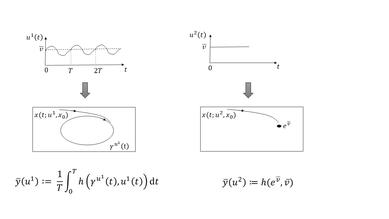
Figure 1: Gain of entrainment (GOE) in a system with output $y=h(x,u)$. Left: $u^{1}(t)$ is a $T$-periodic control and $\gamma^{u^{1}}(t)$, $t\in[0,T)$, is the corresponding EGAS trajectory. Right: $u^{2}(t)\equiv\overline{v}:=\frac{1}{T}\int_{0}^{T}u^{1}(t)\mathop{}\!\mathrm{d}t$ is a constant control and $e^{\overline{v}}$ is the corresponding EGAS equilibrium. The system admits a GOE if $\bar{y}(u^{1})>\bar{y}(u^{2})$.

GOE may be relevant in numerous applications including vehicular control using periodic traffic lights, periodic fishery [5], periodic operation of chemical processes [48], periodic outbreaks of epidemics [31], periodic gene expression [45], and more. All these processes can also be controlled using constant controls, and assessing the GOE can be used to determine if periodic controls are “better” than constnt ones.

Asymptotically stable linear time-invariant (LTI) systems admit no GOE. The next example demonstrates this.

Example 1.

Consider the single-input single-output system:

$$\dot{x}(t) =Ax(t)+bu(t),$$

$$y(t) =c^{T}x(t),$$

where $A$ is a Hurwitz matrix. Let $G:\mathbb{C}\to\mathbb{C}$ denote the transfer function of this system, i.e., $G(s):=c^{T}(sI-A)^{-1}b$. Fix a frequency $\omega>0$, and consider the system response to two controls

$$u(t)\equiv\bar{v},$$

and

$$u(t)+\Delta u(t)=\bar{v}+\sin(\omega t).$$

Let $T:=2\pi/\omega$. For the first control, the output converges to the $T$-periodic solution

$$\gamma^{u}(t)\equiv G(0)\bar{v},$$

and for the second control to

$$\gamma^{u+\Delta u}(t)=G(0)\bar{v}+|G(\mathrm{i}\omega)|\sin\bigl{(}\omega t+\arg G(\mathrm{i}\omega)\bigl{)}.$$ (1)

The average values of these outputs are $\frac{1}{T}\int_{0}^{T}\gamma^{u}(t)\mathop{}\!\mathrm{d}t=G(0)\bar{v},$ and $\frac{1}{T}\int_{0}^{T}\gamma^{u+\Delta u}(t)\mathop{}\!\mathrm{d}t=G(0)\bar{v},$ implying no GOE.

Non-linear systems may admit a GOE. The next example from [37] demonstrates this.

Example 2.

Consider the non-linear system

$$\dot{x}_{1} =-x_{1}+x_{2}^{2},$$

$$\dot{x}_{2} =-x_{2}+u,$$

$$y =x_{1}.$$ (2)

This is the series interconnection of two (scalar) contractive systems (see Section II), and is thus a contractive system [35]. Consider two controls. The first is $u(t)\equiv 0$. For this control the output of (2) converges to the steady-state value $\gamma^{u}(t)\equiv 0$. The second control is $u+\Delta u$, with $\Delta u(t):=a\sin(\omega t)$, where $a,\omega>0$. This control is $T$-periodic for $T:=2\pi/\omega$, and has average $\frac{1}{T}\int_{0}^{T}(u(t)+\Delta u(t))\mathop{}\!\mathrm{d}t=0$. A calculation shows that for this control the output of (2) converges to a peridoic solution $\gamma^{u+\Delta u}$ satisfying

$$2(4\omega^{4}+5\omega^{2}+1)\gamma^{u+\Delta u}(t)=4a^{2}\omega^{2}+a^{2}-2a^{2}\omega\sin(2t\omega-2\tan^{-1}(\omega))-a^{2}\cos(2t\omega-2\tan^{-1}(\omega)),$$ (3)

so

$$\frac{1}{T}\int_{0}^{T}\gamma^{u+\Delta u}(t)\mathop{}\!\mathrm{d}t=\frac{a^{2}}{2(1+\omega^{2})}.$$ (4)

Thus, the GOE for this input is always positive and depends on both the excitation amplitude $a$ and frequency $\omega$. Note that the GOE is quadratic in $a$.

Examples 1 and 2 raise several interesting questions. For example, given a nonlinear system, how can one determine if it admits a GOE and for what controls? What control gives the best possible GOE? Are there systems that have (or do not have) a GOE for any admissible control?

Several recent papers analyzed the GOE in a nonlinear model from systems biology called the ribosome flow model (RFM). This is a non-linear ODE model for the flow of ribosomes and the production of proteins during mRNA translation [34, 1], where the output is the protein production rate. It was shown that, perhaps surprisingly, for several special cases the RFM has no GOE. In other words, $T$-periodic controls are not better than constant ones in terms of maximizing the average protein production rate.

GOE may also be studied in the framework of optimal control theory. The basic idea behind this approach is to pose the problem of finding an admissible control, within the set of $T$-periodic control inputs, which maximizes the average output under: (1) a constraint on the average of the control, and (2) considering the output along the EGAS $T$-periodic solution. However, these constraints make the problem difficult to tackle, and solutions exist only for special cases, e.g., for scalar systems [4, 13].

I-C Contributions of this paper

Motivated by the considerations in the previous subsection, in this paper we rigorously analyze the sensitivity of entrainment and the GOE in a specific class of bilinear and weakly contractive systems. The main contributions of this paper include:

• We analyze the sensitivity function of solutions with respect to a change in the control input. The latter is given as the solution of an ODE on an appropriate infinite-dimensional Banach space. Rather than analyzing this infinite-dimensional ODE directly, we reduce the analysis to an ODE in $\mathbb{R}^{n}$ and employ tools from finite-dimensional systems, thereby making the analysis more accessible to a wider audience;

• We then show that the mapping $u\to\gamma^{u}(0)$ from a periodic control $u$ to the initial value of the corresponding $T$-periodic solution $\gamma^{u}$ admits a Fréchet derivative, and that this derivative is continuous. We derive an explicit expression for the Fréchet derivative. This can be used in conjunction with numerical tools to study various properties of the mapping $u\to\gamma^{u}$. In particular, it provides new formulas that may reduce the numerical work for finding controls that improve the output of the system;

• We show that at constant controls this Fréchet derivative is zero, implying that their GOE is inherently a higher-order phenomenon in the norm of the control perturbation. We consider this a surprising phenomenon, which is due to the interplay of the first-order terms of the periodic perturbation $\Delta u$ entering the system and the resulting change of the initial condition $\gamma^{u+\Delta u}(0)$ of the corresponding periodic solution, which effectively cancel out in the integrated output;

• We demonstrate these results by applying them to two important mathematical models: the master equation for irreducible finite state Markov processes and the RFM, both with $T$-periodic transition rates. It should be noted that the master equations obey a weak version of contractiveness. Indeed, the equations are only non-expanding in general, and irreducibility of the underlying Markov-process is required to guarantee some form of contraction. Therefore our proofs avoid making unnecessary use of contraction. In fact, we found that entrainment for all admissible controls is the basic assumption, and this must be supplemented by a non-degeneracy condition for the associated Poincaré map.

The remainder of this paper is organized as follows. The next section introduces some notation and several known results that will be used later on. Section III describes the bilinear control system that we analyze. Section IV details our main results. Section V includes the proofs of the main results. Sections VI and VII detail applications of the theoretical results to two models: the RFM and time-varying Markov chains. Section VIII describes a generalization of our results. The final section concludes, and describes possible topics for further research.

II Preliminaries

We begin with a short review on contraction in finite-dimensional ODEs. For more details and proofs, see, e.g., [2, 49, 7].

II-A Contraction in finite-dimensional ODE systems

Consider the nonlinear dynamical system:

$$\begin{array}[]{lll}&\dot{x}(t)=f(x(t),u(t)),\\ &x(0)=x_{0}\in\Omega,\end{array}$$ (5)

with state $x(t)\in\Omega\subseteq\mathbb{R}^{n}$, and control input $u(t)=\begin{bmatrix}u_{1}(t)&\dots&u_{m}(t)\end{bmatrix}^{T}\in U\subseteq\mathbb{R}^{m}$. Let $\mathcal{U}\subseteq Z$ denote the subset of admissible controls, where $Z$ is a Banach space. We assume that the vector field $f\in C^{1}$, and let

$$f_{x}(x,u):=\frac{\partial}{\partial x}f(x,u),\quad f_{u}(x,u):=\frac{\partial}{\partial u}f(x,u),$$

denote its Jacobians with respect to the state and the control, respectively.

For $u\in\mathcal{U}$ and $x_{0}\in\Omega$, let $x(t;u,x_{0})$ denote the solution of (5) at time $t\geq 0$. We say that the system (5) is contractive if there exist $\eta>0$ (called the contraction rate) and a norm $|\cdot|:\mathbb{R}^{n}\to[0,\infty)$ such that for any admissible control $u$, and any two initial conditions $a,b\in\Omega$, we have

$$|x(t;u,a)-x(t;u,b)|\leq\exp(-\eta t)|a-b|,\text{ for all }t\geq 0.$$ (6)

In other words, any two trajectories approach each other at an exponential rate, and this holds uniformly with respect to the controls.

Recall that the norm $|\cdot|:\mathbb{R}^{n}\to[0,\infty)$ induces a matrix norm $\|\cdot\|:\mathbb{R}^{n\times n}\to[0,\infty)$ defined by $\|A\|:=\max_{|x|=1}|Ax|,$ and a matrix measure $\mu:\mathbb{R}^{n\times n}\to\mathbb{R}$ (also called logarithmic norm [53]) defined by

$$\mu(A):=\lim_{\varepsilon\downarrow 0}\frac{\|I_{n}+\varepsilon A\|-1}{\varepsilon}.$$ (7)

Assume that the state space $\Omega$ is forward-invariant, convex and bounded, and that $U\subseteq\mathbb{R}^{m}$ is bounded. Then a sufficient condition for contractivity of (5) is that the matrix measure $\mu:\mathbb{R}^{n\times n}\to\mathbb{R}$ induced by $|\cdot|$ satisfies

$$\mu\left(f_{x}(x,u)\right)\leq-\eta<0\text{ for all }x\in\Omega,u\in U.$$ (8)

In both applications described in this paper, namely, the RFM and time-varying Markov chains, neither (8) nor (6) hold uniformly for all of the forward invariant state space. Therefore we do not use these bounds and their powerful consequences like the input-to-state stability (ISS) property [9, 49]. Instead, we use entrainment to periodic controls as our main hypothesis. This property has already been established for the application systems in this paper, see [27, 25].

II-B Sensitivity functions, abstract ODEs and evolution equations

Recall that $x(t;u,x_{0})$ is the solution of (5) at time $t\geq 0$. Consider the sensitivity function $\frac{\partial x}{\partial x_{0}}(t):=\frac{\partial x}{\partial x_{0}}(t;u,x_{0})$. Formally, $\frac{\partial x}{\partial x_{0}}(t)$ belongs to the set of bounded linear operators from $\mathbb{R}^{n}$ to $\mathbb{R}^{n}$ (and can thus be considered as an $n\times n$ matrix), and describes how a small perturbation in the initial condition $x_{0}$ translates to a change in the solution value $x(t;u,x_{0})$ at time $t$. It is well-known that $\frac{\partial x}{\partial x_{0}}:[0,\infty)\rightarrow\mathbb{R}^{n\times n}$ satisfies the variational (matrix) ODE:

$$\frac{d}{dt}\frac{\partial x(t)}{\partial x_{0}} =f_{x}(x(t),u(t))\frac{\partial x(t)}{\partial x_{0}},$$

$$\frac{\partial x(t)}{\partial x_{0}}(0) =I_{n}.$$

Given a Banach space of controls $Z$ and a set of admissible controls $\mathcal{U}\subseteq Z$, the sensitivity with respect to controls at time $t$ is denoted by $\frac{\partial x(t)}{\partial u}$. Then $\frac{\partial x(t)}{\partial u}\in\mathcal{B}(Z,\mathbb{R}^{n})$, where $\mathcal{B}(Z,\mathbb{R}^{n})$ is the space of bounded linear operators mapping $Z$ to $\mathbb{R}^{n}$. The operator $\frac{\partial x(t)}{\partial u}$ describes how a perturbation in the control input translates to a change in the solution value $x(t;u,x_{0})$. Differently from $\frac{\partial x(t)}{\partial x_{0}}$, the domain of $\frac{\partial x(t)}{\partial u}$ lies in an infinite-dimensional space. Assuming for the moment that $\frac{\partial x}{\partial u}:[0,\infty)\rightarrow\mathcal{B}(Z,\mathbb{R}^{n})$ exists and is differentiable (in an appropriate sense) for all $t\geq 0$, we expect it to satisfy two properties. First, $\frac{\partial x}{\partial u}(0)=0$, as $x(0;u,x_{0})=x_{0}$ does not depend on the control. Second, a formal calculation gives:

$$\frac{d}{dt}\frac{\partial x(t)}{\partial u}=\frac{\partial}{\partial u}f(x(t),u(t))=f_{x}(x(t),u(t))\frac{\partial x(t)}{\partial u}+f_{u}(x(t),u(t)).$$ (9)

These considerations suggest the abstract ODE (evolution equation) over the Banach space $X=\mathcal{B}(Z,\mathbb{R}^{n})$:

$$\dot{\psi}(t) =A(t)\psi(t)+\lambda(t),$$

$$\psi(0) =0,$$ (10)

where $A(t):=f_{x}(x(t),u(t))$ are $n\times n$ matrices and $\lambda(t):=f_{u}(x(t),u(t))$. In (II-B) we interpret $A(t)$ as a map $\mathcal{B}(Z,\mathbb{R}^{n})\ni\psi\mapsto A(t)\psi\in\mathcal{B}(Z,\mathbb{R}^{n})$; that is for all $z\in Z$, $\left[A(t)\psi\right](z)=A(t)\psi(z)$. If $f(x,u)$ satisfies the infinitesimal condition for contraction (8) then, by definition, so does $A(t)$ in (II-B).

The study of evolution equations of the form (II-B) relies on the theory of $C_{0}$ semigroups of bounded linear operators and their generators, see, e.g., [38]. Yet, in this paper we prove existence and uniqueness of a classical solution to (9), for a class of weakly contractive bilinear control systems, using an alternative approach that is more tractable and, in particular, involves only finite-dimensional ODEs. Indeed, for $\Delta u\in Z$, set $z(t):=\frac{\partial x(t)}{\partial u}\Delta u\in\mathbb{R}^{n}$. Then $z(t)$ is the solution of the finite-dimensional system $\dot{z}(t)=A(t)z(t)+\lambda(t)\Delta u(t)$ with zero initial condition. However, this is only true if existence of $\frac{\partial x(t)}{\partial u}$ has been established. Below, we will consider the system for $z(t)$ as a starting point and prove that $B(t):\Delta u\mapsto z(t)$ is a bounded linear map, which is a candidate for $\frac{\partial x(t)}{\partial u}$. We then show that

$$x(t;u+\Delta u,x_{0})=x(t;u,x_{0})+B(t)\Delta u+o(\left\|\Delta u\right\|_{Z}),$$

which demonstrates that indeed $B(t)=\frac{\partial x(t)}{\partial u}$ is the Fréchet derivative. This proof strategy relies only on tools from finite-dimensional systems. For contraction analysis of infinite-dimensional systems, see [52] and the references therein.

II-C An implicit function theorem on Banach spaces

The following implicit function theorem will be central to our analysis (see e.g. [10, Section VI.2] and [44, Section 4]):

Theorem 1.

[Implicit function theorem on Banach space.] Let $M$, $N$, and $G$ be Banach spaces. Let $D\subseteq M\times N$ be an open set, and let $f:D\to G$ be a continuously Fréchet differentiable mapping. Assume that for some $(a,b)\in D$, we have $f(a,b)=0$ and that the Fréchet derivative $d_{n}f(a,b):N\to G$ is a bijection. Then there exists a neighborhood $W_{a}\subseteq M$ of $a$, a neighborhood $W_{b}\subseteq N$ of $b$ and a continuously Fréchet differentiable mapping $g:W_{a}\to W_{b}$ such that

$$f(x,y)=0\iff y=g(x),\text{ for all }(x,y)\in W_{a}\times W_{b}.$$

III The model

In this section, we describe the bilinear control system that we consider, and our standing assumptions. The control system is of the form

$$\dot{x}(t) =f(u(t))+M(x(t))u(t),$$ (11)

$$y(t) =h(u(t),x(t)),$$

and we denote by $x(t;u,x_{0})$ the solution of (11) that satisfies in addition the initial condition $x(0)=x_{0}$. Note that (11) is not the standard affine in the control system, as the “drift vector” $f$ depends on $u$ and not on $x$. However, as shown in Sections VI and VII, several important real-world models can be written in the form (11). Also, an extension of our results to more general models is described in Section VIII.

We begin by defining the ambient space $Z$ for the set of admissible controls $u(t)\in\mathbb{R}^{m}$. Given $T>0$, let $Z:=C_{\text{Per}}(0,T)$ denote the space of continuous functions $g:[0,T]\rightarrow\mathbb{R}^{m}$ satisfying $g_{i}(0)=g_{i}(T)$ for all $i=1,\dots,m$. Then any $g\in Z$ can be extended to a continuous function on $[0,\infty)$ via periodicity, and it is this extension that is used in the control system (11). The set $Z$, equipped with the norm

$$\left\|g\right\|_{Z}:=\max_{i=1,\dots,m}\;\max_{t\in[0,T]}|g_{i}(t)|,$$

is a Banach space. We are now ready to formulate our assumptions on the functions appearing in the control system (11) with state space in $\mathbb{R}^{n}$ and scalar output $y$.

III-A General Assumptions

There exist nonempty, open sets $\Omega\subset\mathbb{R}^{n}$ and $\mathcal{U}\subset Z$ such that conditions (C1) – (C3) hold.

• Regularity. The maps $f:\mathbb{R}^{m}\rightarrow\mathbb{R}^{n}$, $M:\Omega\to\mathbb{R}^{n\times m}$, and $h:\mathbb{R}^{m}\times\Omega\rightarrow\mathbb{R}$ are continuously differentiable.

• Entrainment. For every $u\in\mathcal{U}$ system (11) has a unique $T$-periodic solution $\gamma^{u}$ in $\Omega$.

• Non-degeneracy. For every $u\in\mathcal{U}$ the sensitivity function $\frac{\partial x}{\partial x_{0}}(T;u,\gamma^{u}(0))$ at time $T$ for the periodic solution $\gamma^{u}$ does not have $1$ as an eigenvalue.

III-B Discussion of the Assumptions and first conclusions

We now describe a setting in which our general assumptions are always satisfied. Suppose we have a contractive system in the sense that the bound (6) holds for all $a$, $b$ in a compact and forward invariant subset $K\subset\mathbb{R}^{n}$ and for all admissible controls $u\in\mathcal{U}$. Let us further assume that the boundary of $K$ is repelling in the sense that solutions cannot remain in $\partial K$ for all times $t\geq 0$ and that a solution that lies in the interior of $K$ at some time $t^{*}$ will stay there for all times $t>t^{*}$. Then the interior $\Omega:=\operatorname{Int}(K)$ of $K$ is also forward invariant and condition (C2) is satisfied. Indeed, as the Poincaré maps $P^{u}:K\to K$ defined by $P^{u}(x_{0}):=x(T;u,x_{0})$ is a contraction on $K$ there exists for every admissible control $u$ a unique fixed point ${x}^{u}\in K$ of $P^{u}$. The solution starting in ${x}^{u}$ at time $0$ provides the unique periodic solution $\gamma^{u}$. The assumption of a repelling boundary as detailed above implies that all of $\gamma^{u}$ lies in $\Omega$. Condition (C3) can be verified by contradiction. If there exists $u\in\mathcal{U}$ and an eigenvector $v\in\mathbb{R}^{n}\setminus\{0\}$ with $\frac{\partial x}{\partial x_{0}}(T;u,\gamma^{u}(0))v=v$, then inequality (6) is violated for $t=T$, $a=\gamma^{u}(0)$, and $b=\gamma^{u}(0)+\varepsilon v$ for $\varepsilon$ sufficiently small.

The conditions that we have posed as general assumptions are weaker than the one described in Subsection II-A. Our choice of conditions was motivated by the applications described in Sections VI and VII below. A crucial ingredient for the proofs of our main results, which follows from our general assumptions, is stated in the following proposition.

Proposition 2.

Assume conditions (C1) – (C3) hold. Fix $u_{0}\in\mathcal{U}$. Then there exist numbers $d$, $r_{x}$, $r_{u}>0$ such that for all $(u,x_{0})$ in the open set $\mathcal{D}_{u_{0}}:=B(u_{0},r_{u})\times B(\gamma^{u_{0}}(0),r_{x})\subset\Omega\times\mathcal{U}$ the solution $x(t;u,x_{0})$ of system (11) with initial condition $x(0)=x_{0}$ stays within a compact set $K_{u_{0}}\subset\Omega$ for all times $t\in[0,T]$. Moreover, for all $(u,x_{0})$, $(\tilde{u},\tilde{x}_{0})\in\mathcal{D}_{u_{0}}$ and $t\in[0,T]$ we have

$$|x(t;u,x_{0})-x(t;\tilde{u},\tilde{x}_{0})|\leq d\left(|x_{0}-\tilde{x}_{0}|+\|u-\tilde{u}\|_{Z}\right).$$ (12)

Finally, for constant controls $u_{0}(t)\equiv\bar{v}$ with $u_{0}\in\mathcal{U}$, we have that $\gamma^{u_{0}}(t)\equiv e^{\bar{v}}$, that is, an equilibrium point.

Proof.

Choose $\varepsilon>0$ such that the closure $K_{u_{0}}$ of the $\varepsilon$-neighborhood $\Omega_{\varepsilon}:=\cup_{t\in[0,T]}B(\gamma^{u_{0}}(t),\varepsilon)$ of the compact set $\gamma^{u_{0}}([0,T])$ is contained in $\Omega$. For $x_{0}\in B(\gamma^{u_{0}}(0),\varepsilon)$ and $u\in B(u_{0},1)$ we consider the difference $\Delta x(t):=x(t;u,x_{0})-\gamma^{u_{0}}(t)$ for $t\in[0,T^{*})$ with $T^{*}=T^{*}(u,x_{0})$ chosen so that $[0,T^{*})$ is the maximal interval for which $|\Delta x(t)|<\varepsilon$ holds. Let

$$J(x,u):=\frac{\partial M(x)}{\partial x}u$$ (13)

denote the Jacobian of the vector field in (11) with respect to $x$. Then $\Delta x$ satisfies the linear initial value problem

$$\frac{d}{dt}\Delta x(t) =A(t)\Delta x(t)+b(t),$$

$$\Delta x(0) =x_{0}-\gamma^{u_{0}}(0)$$

with

$$A(t) :=\int_{0}^{1}J(\gamma^{u_{0}}(t)+r\Delta x(t),u_{0}(t))\mathop{}\!\mathrm{d}r,$$

$$b(t) :=f(u(t))-f(u_{0}(t))+M(x(t;u,x_{0}))\bigl{(}u(t)-u_{0}(t)\bigl{)},$$

where we used the fact that $A(t)\Delta x(t)=\bigl{(}M(x(t;u;x_{0}))-M(\gamma^{u_{0}}(t))\bigl{)}u_{0}(t)$ by the fundamental theorem of calculus, and the convexity of the balls $B(\gamma^{u_{0}}(t),\varepsilon)$. Condition (C1) together with the compactness of $K_{u_{0}}$ implies that there exists a constant $d^{\prime}=d^{\prime}(u_{0})>0$ such that $|b(t)|\leq d^{\prime}\|u-u_{0}\|_{Z}$ for all $u\in B(u_{0},1)$. Moreover, for all $r\in[0,1]$, $t\in[0,T^{*})$ the argument $(\gamma^{u_{0}}(t)+r\Delta x(t),u_{0}(t))$ of the continuous map $J$ in the definition of $A(t)$ is contained in some compact set $K_{u_{0}}\times\hat{K}_{u_{0}}\subset\Omega\times\mathbb{R}^{m}$ that only depends on $u_{0}$. Thus there exists a constant $\hat{d}=\hat{d}(u_{0})>0$ such that the transfer matrix $\Phi(t;s)$ of the linear time-varying system $\dot{z}=A(t)z$ satisfies $\|\Phi(t;s)\|\leq\hat{d}$ for $0\leq s\leq t<T^{*}$. By the variation of constants formula we have

$$\Delta x(t)=\Phi(t;0)\left(x_{0}-\gamma^{u_{0}}(0)\right)+\int_{0}^{t}\Phi(t;s)b(s)\mathop{}\!\mathrm{d}s$$

and therefore

$$|\Delta x(t)|\leq\hat{d}\,|x_{0}-\gamma^{u_{0}}(0)|\,+\,t\hat{d}d^{\prime}\,\|u-u_{0}\|_{Z},\text{ for all }t\in[0,T^{*}).$$ (14)

Choosing $r_{u}:=\min\{\varepsilon/(2T\hat{d}d^{\prime}),1\}$ and $r_{x}:=\min\{1/\hat{d},1\}\varepsilon/2$ ensures that the solution $x(t;u,x_{0})$ cannot leave the neighborhood $\Omega_{\varepsilon}$ for $t\in[0,T]$. In other words $T^{*}>T$.

In order to prove the bound (12) we proceed as above, with the only difference that we replace $u_{0}$ by $\tilde{u}$ and, consequently, $\gamma^{u_{0}}(0)$ by $\tilde{x}_{0}$ and $\gamma^{u_{0}}(t)$ by $x(t;\tilde{u},\tilde{x}_{0})$. Observe that the convexity of the balls $B(\gamma^{u_{0}}(t),\varepsilon)$ implies that the interpolations $rx(t;u,x_{0})+(1-r)x(t;\tilde{u},\tilde{x}_{0})$, $0\leq r\leq 1$, that appear in the analogue formula for matrix $A(t)$ above are still contained in the set $\Omega_{\varepsilon}\subset\Omega$. One may again derive estimate (14) with constants $d^{\prime}$, $\hat{d}$ only depending on $u_{0}$. Choosing $d:=\hat{d}\max\{Td^{\prime},1\}$ yields claim (12).

For a constant control $u_{0}\equiv\bar{v}$ system (11) is autonomous and $Y(t):=\frac{d}{dt}\gamma^{u_{0}}(t)$ solves the initial value problem

$$\dot{Y}(t) =J\bigl{(}\gamma^{u_{0}}(t),\bar{v}\bigl{)}Y(t),$$

$$Y(0) =\frac{d}{dt}\gamma^{u_{0}}(0).$$

Observe that the fundamental matrix $\Phi(t)$ for this system, with $\Phi(0)=I_{n}$, equals the sensitivity function $\frac{\partial x}{\partial x_{0}}(t;u_{0},\bar{v})$. Using periodicity of $\gamma^{u_{0}}$ gives $Y(0)=Y(T)=\Phi(T)Y(0)$. Condition (C3) implies that $Y(0)=0$ because $1$ is not an eigenvalue of $\Phi(T)$. Thus $Y(t)=\Phi(t)Y(0)=0$ for all $t\in[0,T]$. This shows that $\gamma^{u_{0}}(t)$ is a constant function. ∎

III-C The map $\Gamma:u\mapsto\gamma^{u}(0)$ and a Poincaré-type map

According to condition (C2) we can uniquely define $\Gamma:\mathcal{U}\rightarrow\Omega$ by

$$\Gamma(u):=\gamma^{u}(0),$$ (15)

that maps a $T$-periodic control to the initial condition at time zero of the corresponding $T$-periodic solution. It is crucial for our analysis to prove differentiability of the map $\Gamma$ and to find an expression for its derivative. The key observation to achieve this is that for every $u\in\mathcal{U}$, we have $\Gamma(u)=\gamma^{u}(T)=x(T;u,\Gamma(u))$. This relation characterizes $\Gamma(u)$, as we have assumed the uniqueness of the periodic solution for any admissible control. Thus $\Gamma(u)$ is the unique zero of the Poincaré-type map $P:\mathcal{D}\to\mathbb{R}^{n}$ defined by

$$P(u,x_{0}):=x(T;u,x_{0})-x_{0},$$ (16)

with $\mathcal{D}:=\bigcup_{u\in\mathcal{U}}\mathcal{D}_{u}$, where the open sets $\mathcal{D}_{u}\subset\mathcal{U}\times\Omega$ are defined as in Proposition 2.

Let us revisit previous examples where we can read off $\Gamma(u)$ for some controls $u$ from the explicit solution formulas. In Example 1 above, we find that for the controls $u,u+\Delta u$ defined there, we have

$$\Gamma(u)=G(0)\bar{v},\qquad\Gamma(u+\Delta u)=G(0)\bar{v}+\operatorname{Im}(G(\mathrm{i}\omega)).$$

Similarly, in Example 2, we obtain

$$\Gamma(u)=0,\qquad\Gamma(u+\Delta u)=\frac{a^{2}\omega^{2}(2\omega^{2}+5)}{(\omega^{2}+1)^{2}(4\omega^{2}+1)}.$$

We conclude this section with a very simple example that satisfies conditions (C1) – (C3).

Example 3.

Consider the scalar equation with state space $\Omega=\mathbb{R}$

$$\dot{x}=-ux,$$ (17)

where $u(t)$ takes values in $(c,\infty)$, $c>0$, for all $t\geq 0$. This is in the form (11) with $n=m=1$, $f=0$, and $M(x)=-x$. The solution of (17) is given by

$$x(t;u,x_{0})=\exp(-w(t))x_{0},$$ (18)

with $w(t):=\int_{0}^{t}u(s)\mathop{}\!\mathrm{d}s$. As $w(T)>0$, condition (C3) holds. Moreover,

$$P(u,x_{0}):=x(T;u,x_{0})-x_{0}=\bigl{(}\exp(-w(T))-1\bigl{)}x_{0}.$$

yields that the Poincaré-type map $P(u,\cdot)$ has a unique zero $\Gamma(u)=0$, so condition (C2) holds. Finally, in this case we can compute the derivatives of $P$ explicitly,

$$\frac{\partial P}{\partial x_{0}}(u,x_{0})=\exp(-w(T))-1\,,\qquad\frac{\partial P}{\partial u}(u,x_{0})\Delta u=\exp(-w(T))x_{0}\left(-\int_{0}^{T}\Delta u(s)\mathop{}\!\mathrm{d}s\right)$$

for $\Delta u\in Z$ $($recall that $\frac{\partial P}{\partial u}(u,x_{0})$ lies in $\mathcal{B}(Z,\mathbb{R}))$. The second formula can be derived from

$$x(T;u+\Delta u,x_{0})-x(T;u,x_{0}) =\left(\exp(-\int_{0}^{T}\Delta u(s)\mathop{}\!\mathrm{d}s)-1\right)\exp(-w(T))x_{0}$$

$$=\left(-\int_{0}^{T}\Delta u(s)\mathop{}\!\mathrm{d}s\right)\exp(-w(T))x_{0}+o(\|\Delta u\|_{Z}),$$

where $o(\epsilon)$ denotes the set of functions $g:\mathbb{R}_{+}\to\mathbb{R}$ satisfying $\lim_{\epsilon\to 0^{+}}\frac{g(\epsilon)}{\epsilon}=0.$

IV Main results

This section describes the main results. All the proofs are placed in the next section. Throughout the present section we assume that the general assumptions of Section III-A are satisfied. Moreover, we use freely the notation introduced in Proposition 2 and the definitions provided by (15) and (16).

Modifying a control $u$ to $u+\Delta u$ generates a change from $\gamma^{u}$ to $\gamma^{u+\Delta u}$. Since $\Gamma(u)$ and $\Gamma(u+\Delta u)$ are the initial condition of these periodic solutions, respectively, it is important to know the derivative of $\Gamma$. The next result provides an explicit expression for this quantity.

Theorem 3 (Explicit expression for the derivative of $\Gamma$).

Consider the system (11) . Then the mapping $\Gamma$ in (15) is continuously Fréchet differentiable, and its Fréchet derivative $d\Gamma(u)\in\mathcal{B}(Z,\mathbb{R}^{n})$ is given by

$$d\Gamma(u)\Delta u =-\left(\frac{\partial x}{\partial x_{0}}(T;u,\Gamma(u))-I_{n}\right)^{-1}\frac{\partial x}{\partial u}(T;u,\Gamma(u))\Delta u$$

$$=-\left(\Phi_{u,\Gamma(u)}(T;0)-I_{n}\right)^{-1}\int_{0}^{T}\Phi_{u,\Gamma(u)}(T;s)\Bigl{(}M(\gamma^{u}(s))+Df(u(s))\Bigl{)}\Delta u(s)\mathop{}\!\mathrm{d}s$$ (19)

for all $\Delta u\in Z$. Here $\Phi_{u,x_{0}}(t;t_{0})$ is the solution at time $t$ of the linear time-varying matrix ODE:

$$\dot{\Phi}(\tau) =J\bigl{(}x(\tau;u,x_{0}),u(\tau)\bigl{)}\Phi(\tau),$$

$$\Phi(t_{0}) =I_{n}$$ (20)

with $J$ from (13).

Example 4.

Consider again the system in Example 3. For this system, Eq. (3) gives

$$d\Gamma(u)\Delta u =-\left(\frac{\partial x}{\partial x_{0}}(T;u,\Gamma(u))-I_{n}\right)^{-1}\frac{\partial x}{\partial u}(T;u,\Gamma(u))\Delta u$$

$$=-\left(\exp(-w(T))-1\right)^{-1}\bigl{(}-\int_{0}^{T}\Delta u(s)\mathop{}\!\mathrm{d}s\bigl{)}\exp(-w(T))\Gamma(u)$$

$$=0,$$

and this is correct, as in this case $\Gamma(u)\equiv 0$.

Remark 1.

Pavlov et al. [37] considered the more general class of convergent systems and showed that for such systems the map $u\mapsto\gamma^{u}$ is continuous. Theorem 3 shows that for the class of systems we study, and assuming that conditions (C1)–(C3) hold, $\Gamma$ satisfies a stronger regularity condition. Furthermore, as we will see below the explicit expression for $d\Gamma$ plays a crucial role in the analysis of the GOE. We note that Pavlov et al. [37] did not assume condition (C3), but it is possible to demonstrate that this condition is necessary to guarantee that Theorem 3 holds.

The next result analyzes $d\Gamma(u)$ in the particular case where $u$ is a constant control.

Corollary 4.

Let $u(t)\equiv\bar{v}$ be a constant control in $\mathcal{U}$. Denote by $e^{\bar{v}}$ the corresponding equilibrium point of the system according to Proposition 2 so, in particular, $\Gamma(u)=e^{\bar{v}}$. Let $H:=J(e^{\bar{v}},\bar{v})$. Then

$$d\Gamma(u)\Delta u=-\left(\exp(HT)-I_{n}\right)^{-1}\int_{0}^{T}\exp\left(H(T-s)\right)\left(M(e^{\bar{v}})+{Df(\bar{v})}\right)\Delta u(s)\mathop{}\!\mathrm{d}s$$ (21)

for any $\Delta u\in Z$.

The next result considers the difference in the outputs along the periodic solutions corresponding to two controls: $u$ and $u+\Delta u$.

Theorem 5 (A first-order expression for the GOE).

Consider the system (11). Fix $u\in\mathcal{U}$. For all $u+\Delta u$ with $(u+\Delta u,\Gamma(u+\Delta u))\in\mathcal{D}_{u}$ let $\gamma^{u}$ and $\gamma^{u+\Delta u}$ denote the corresponding $T$-periodic solutions, and consider the outputs

$$y^{u}(t) :=h\left(u(t),\gamma^{u}(t)\right),$$

$$y^{u+\Delta u}(t) :=h\left(u(t)+\Delta u(t),\gamma^{u+\Delta u}(t)\right).$$ (22)

Let

$$\overline{y^{u+\Delta u}-y^{u}}:=\frac{1}{T}\int_{0}^{T}\left(y^{u+\Delta u}(t)-y^{u}(t)\right)\mathop{}\!\mathrm{d}t$$

denote the difference in the average of these outputs. Then

$$\overline{y^{u+\Delta u}-y^{u}} =\frac{1}{T}\int_{0}^{T}\frac{\partial h}{\partial u}(u(t),\gamma^{u}(t))\Delta u(t)\mathop{}\!\mathrm{d}t$$

$$+\frac{1}{T}\int_{0}^{T}\frac{\partial h}{\partial x}(u(t),\gamma^{u}(t))\left(\frac{\partial x}{\partial x_{0}}(t;u,\Gamma(u))d\Gamma(u)\Delta u+\frac{\partial x}{\partial u}(t;u,\Gamma(u))\Delta u\right)\mathop{}\!\mathrm{d}t$$

$$+o(\left\|\Delta u\right\|_{Z}).$$ (23)

Remark 2.

Given $u\in\mathcal{U}$, it is often of interest to numerically verify whether a $T$-periodic perturbation $\Delta u$ in the control yields an increase in the average output. A straightforward approach is to use a numerical ODE solver to converge to the solutions $\gamma^{u}$ and $\gamma^{u+\Delta u}$ and then numerically compute the average of the difference $y^{\gamma+\Delta\gamma}-y^{\gamma}$. However, if the system dimension and/or the set of candidate perturbations are large, this may be a costly procedure.

Combining Theorem 5 with the explicit expressions derived for $\frac{\partial x}{\partial x_{0}}(t;u,\Gamma(u))$, $\frac{\partial x}{\partial u}(t;u,\Gamma(u))$ and $d\Gamma(u)$ yields, via Fubini’s theorem, the following kernel representation

$$\overline{y^{u+\Delta u}-y^{u}} =\frac{1}{T}\int_{0}^{T}\mathcal{K}(t)\Delta u(t)\mathop{}\!\mathrm{d}t+o(\left\|\Delta u\right\|_{Z}),$$ (24)

where

$$\mathcal{K}(t) :=\frac{\partial h}{\partial u}(u(t),\gamma^{u}(t))-\left(\int_{0}^{T}\frac{\partial h}{\partial x}(u(s),\gamma^{u}(s)\Phi_{u,\Gamma(u)}(s;0))\mathop{}\!\mathrm{d}s\right)\left(\Phi_{u,\Gamma(u)}(T;0)-I_{n}\right)^{-1}$$

$$\times\Phi_{u,\Gamma(u)}(T;t)\Bigl{(}M(\gamma^{u}(t))+Df(u(t))\Bigl{)}+\left(\int_{t}^{T}\frac{\partial h}{\partial x}(u(s),\gamma^{u}(s))\Phi_{u,\Gamma(u)}(s;t)\mathop{}\!\mathrm{d}s\right)$$

$$\times\Bigl{(}M(\gamma^{u}(t))+Df(u(t))\Bigl{)}.$$

The latter suggests an approach for maximizing the GOE (to first order). Indeed, for $\left\|\Delta u\right\|_{Z}\leq 1$, we have

$$\left|\frac{1}{T}\int_{0}^{T}\mathcal{K}(t)\Delta u(t)\mathop{}\!\mathrm{d}t\right|\leq\frac{1}{T}\int_{0}^{T}\left|\mathcal{K}(t)\right|_{1}\mathop{}\!\mathrm{d}t.$$

Thus, to increase the first term on the right-hand side of (24), one can take $\Delta u\in Z$ which approximates $\operatorname{sgn}(\mathcal{K}(t))^{\top}=\left(\operatorname{sgn}(\mathcal{K}_{1}(t)),\dots,\operatorname{sgn}(\mathcal{K}_{m}(t))\right)^{\top}$ on $[0,T]$. Note that the numerical approximation of $\mathcal{K}$ requires computing only $\gamma^{u}$ and $\Phi_{u,\Gamma(u)}$.

The next result uses Corollary 4 to analyze the GOE in the vicinity of a constant control.

Theorem 6 (GOE w.r.t. a constant control is a higher-order phenomenon).

Consider the system (11). Fix a constant control $u(t)\equiv\bar{v}$, and let $e^{\bar{v}}$ denote the corresponding equilibrium point. For all $u+\Delta u$ with $(u+\Delta u,\Gamma(u+\Delta u))$, let $\gamma^{u+\Delta u}$ denote the corresponding $T$-periodic solution. Let

$$\begin{array}[]{lll}&y^{u}(t):=h(\bar{v},e^{\bar{v}}),\\ &y^{u+\Delta u}(t):=h\left(u(t)+\Delta u(t),\gamma^{u+\Delta u}(t)\right),\quad t\in[0,T),\end{array}$$ (25)

that is, the outputs along the constant and $T$-periodic solution, respectively. Then for any $\Delta u$, such that $\overline{\Delta u}:=\frac{1}{T}\int_{0}^{T}\Delta u(t)\mathop{}\!\mathrm{d}t=0$, we have

$$\frac{1}{T}\int_{0}^{T}\left(y^{u+\Delta u}(t)-y^{u}(t)\right)\mathop{}\!\mathrm{d}t=o(\|\Delta u\|_{Z}).$$ (26)

To explain why this result is important, assume for a moment that

$$\frac{1}{T}\int_{0}^{T}\left(y^{u+\Delta u}(t)-y^{u}(t)\right)\mathop{}\!\mathrm{d}t=r(\Delta u)+o(\|\Delta u\|_{Z}),$$

where $r:Z\to\mathbb{R}$ is linear in $\Delta u$, and $r(\Delta u)\not=0$. This would imply that either the perturbation $\Delta u$ or $-\Delta u$ always yields a GOE. Theorem 6 states that the linear term $r(\Delta u)$ is zero. Thus, the problem of finding a control that yields a GOE, if it exists, is non trivial. Furthermore, Theorem 6 implies that the GOE for constant controls is determined by terms that are at least second-order in $\Delta u$, suggesting that the study of GOE may be related to some form of “convexity” of higher-order operators (see [21] for some related considerations).

V Proofs

We begin with the proof of Theorem 3. This requires several auxiliary results.

V-A Analysis of the partial derivatives $\frac{\partial x}{\partial u}(t;u,x_{0})$ and $\frac{\partial x}{\partial x_{0}}(t;u,x_{0})$

The partial derivative $\frac{\partial x}{\partial u}(t;u,x_{0})$ is a bounded linear operator and an element of $\mathcal{B}(Z,\mathbb{R}^{n})$. It satisfies an abstract ODE in this space. However, as explained in Section II-B we begin by considering the time evolution of the directional derivatives $\frac{\partial x}{\partial u}(t;u,x_{0})\phi\in\mathbb{R}^{n}$ for $\phi\in Z$ and discuss the question of Fréchet differentiability later. The presented analysis is inspired by the discussion on “linearizations compute differentials” in [50, Section 2.8].

More precisely, fix $u_{0}\in\mathcal{U}$. We seek to determine $\frac{\partial x}{\partial u}(t;u,x_{0})\phi$ for $t\in[0,T]$ and $(u,x_{0})$ in the neighborhood $\mathcal{D}_{u_{0}}$ of $(u_{0},\gamma^{u_{0}}(0))$ specified in Proposition 2. The direction $\phi$ is represented by $\Delta u\in Z$ where $(u+\Delta u,x_{0})$ is also required to lie in $\mathcal{D}_{u_{0}}$. We consider the difference of the two corresponding solutions

$$\Delta x(t):=x(t;u+\Delta u,x_{0})-x(t;u,x_{0}).$$

To simplify the notation, let $x(t):=x(t;u,x_{0})$, $\tilde{u}(t):=u(t)+\Delta u(t)$, $\tilde{x}(t):=x(t;\tilde{u},x_{0})$. Proceeding as in the derivation of (12) in Proposition 2 we obtain

$$\frac{d}{dt}\Delta x(t) =A(t)\Delta x(t)+b(t),$$

$$\Delta x(0) =0,$$

with

$$A(t) =\int_{0}^{1}J(x(t)+r\Delta x(t),u(t))dr,$$

$$b(t) =f(\tilde{u}(t))-f(u(t))+M(\tilde{x}(t))\Delta u(t).$$

Moreover, Proposition 2 provides a constant $d>0$ only depending on the choice of $u_{0}$ such that

$$|\Delta x(t)|\leq d\|\Delta u\|_{Z},\text{ for all }t\in[0,T].$$ (27)

It is our task to find, in an appropriate sense, the best approximation $z$ for $\Delta x$ that depends linearly on $\Delta u$ for the given pair $(u,x_{0})\in\mathcal{D}_{u_{0}}$. Rewrite the above initial value problem in the form

$$\frac{d}{dt}\Delta x(t) =A_{0}(t)\Delta x(t)+b_{0}(t)+R(t),$$

$$\Delta x(0) =0,$$

with

$$A_{0}(t) :=J(x(t),u(t)),$$

$$b_{0}(t) :=Df(u(t))\Delta u(t)+M(x(t))\Delta u(t),$$

$$R(t) :=b(t)-b_{0}(t)+(A(t)-A_{0}(t))\Delta x(t).$$

Observe that $A_{0}$ does not depend on $\Delta u$ and that $b_{0}$ is a linear function of $\Delta u$. As we see below $R$ collects terms that are of higher order in $\Delta u$. This suggests that the best approximation $z$ should satisfy the initial value problem

$$\dot{z} =A_{0}(t)z+b_{0}(t),$$

$$z(0) =0,$$

and this is the same equation that is derived by an abstract approach at the end of Section II-B, although with different notation. Recalling the definition of the transfer matrix $\Phi_{u,x_{0}}(t;t_{0})$ in (3) the solution $z$ of the initial value problem is given by

$$z(t)=\int_{0}^{t}\Phi_{u,x_{0}}(t;s)\Bigl{(}M(x(s;u,x_{0}))+Df(u(s))\Bigl{)}\Delta u(s)\mathop{}\!\mathrm{d}s$$ (28)

and depends linearly on $\Delta u$. Finally, we bound the deviation $e:=\Delta x-z$. We use that $e$ solves the initial value problem

$$\dot{e}(t) =A_{0}(t)e(t)+R(t),$$

$$e(0) =0,$$

together with the representation

$$R(t) =\left[\int_{0}^{1}Df(u(t)+r\Delta u(t))-Df(u(t))\mathop{}\!\mathrm{d}r\right]\Delta u(t)$$

$$+\left[\int_{0}^{1}J(x(t)+r\Delta x(t),\Delta u(t))\mathop{}\!\mathrm{d}r\right]\Delta u(t)$$

$$+\left[\int_{0}^{1}J(x(t)+r\Delta x(t),u(t))-J(x(t),u(t))\mathop{}\!\mathrm{d}r\right]\Delta x(t).$$

For $0\leq r\leq 1$ we have by construction that $x(t)+r\Delta x(t)$ is contained in the compact set $K_{u_{0}}$ obtained in Proposition 2 and $u(t)+r\Delta u(t)$ lies in some compact subset of $\mathbb{R}^{m}$. Condition (C1) thus implies uniform continuity of $Df$ and $J$ and the boundedness of $J$. Together with inequality (27) and the linearity of $J$ in the second argument we conclude $R(t)=o(\|\Delta u\|_{Z})$ uniformly for all $t\in[0,T]$. Since $e(t)=\int_{0}^{t}\Phi_{u,x_{0}}(t;s)R(s)\mathop{}\!\mathrm{d}s$ we learn that $e(t)=o(\|\Delta u\|_{Z})$ uniformly for all $t\in[0,T]$. We summarize our findings.

Proposition 7.

Fix $u_{0}\in\mathcal{U}$ and denote by $\mathcal{D}_{u_{0}}$ the open set in $\mathcal{U}\times\Omega$ specified in Proposition 2. For any $(u,x_{0})\in\mathcal{D}_{u_{0}}$ and $\Delta u\in Z$ with $(u+\Delta u,x_{0})\in\mathcal{D}_{u_{0}}$, we have

$$x(t;u+\Delta u,x_{0})=x(t;u,x_{0})+z(t)+o(\left\|\Delta u\right\|_{Z}),\text{ uniformly over }t\in[0,T],$$ (29)

where $z(t)$, given in (28), is linear in $\Delta u$. In particular, $x(t;u,x_{0})$ is Fréchet differentiable with respect to $u$ and $z(t)=\frac{\partial x}{\partial u}(t;u,x_{0})\Delta u$. Moreover, $z$ solves the initial value problem

$$\dot{z}(t) =J(x(t;u,x_{0}),u(t))z(t)+\Bigl{(}M(x(t;u,x_{0}))+Df(u(t))\Bigl{)}\Delta u(t),$$ (30)

$$z(0) =0.$$

The next result describes the continuity of $\frac{\partial x}{\partial u}(t;u.x_{0})$ as a function of the initial condition $x_{0}$ and control $u$.

Proposition 8.

Fix $u_{0}\in\mathcal{U}$ and denote by $\mathcal{D}_{u_{0}}$ the open set in $\mathcal{U}\times\Omega$ specified in Proposition 2. The mapping $\mathcal{D}_{u_{0}}\ni(u,x_{0})\mapsto\frac{\partial x}{\partial u}(t;u,x_{0})\in\mathcal{B}(Z,\mathbb{R}^{n})$ is continuous, uniformly in $t\in[0,T]$, i.e., for any $(u,x_{0})\in\mathcal{D}_{u_{0}}$, we have

$$\lim_{\begin{subarray}{c}\tilde{u}\to u\\ \tilde{x}_{0}\to x_{0}\end{subarray}}\left(\sup_{t\in[0,T]}\left\|\frac{\partial x}{\partial u}(t;\tilde{u},\tilde{x}_{0})-\frac{\partial x}{\partial u}(t;u,x_{0})\right\|_{\mathcal{B}(Z,\mathbb{R}^{n})}\right)=0.$$

Proof.

Fix $(u,x_{0})\in\mathcal{D}_{u_{0}}$. Let $\Delta x_{0}\in\mathbb{R}^{n}$ and $\Delta u\in Z$ be small enough such that  $\tilde{x}_{0}:=x_{0}+\Delta x_{0}$ and $\tilde{u}:=u+\Delta u$ satisfy $(\tilde{u},\tilde{x}_{0})\in\mathcal{D}_{u_{0}}$. To simplify the notation, set

$$x(t):=x(t;u,x_{0}),\quad\tilde{x}(t):=x(t;\tilde{u},\tilde{x}_{0}).$$

Let $\phi\in Z$ with $\left\|\phi\right\|_{Z}=1$ . Recalling (3) and (28), we define for all $t\in[0,T]$

$$n(t) :=\frac{\partial x}{\partial u}(t;u,x_{0})\phi=\int_{0}^{t}\Phi_{u,x_{0}}(t;s)\Bigl{(}M(x(s))+Df(u(s))\Bigl{)}\phi(s)\text{d}s,$$

$$\tilde{n}(t) :=\frac{\partial x}{\partial u}(t;\tilde{u},\tilde{x}_{0})\phi=\int_{0}^{t}\Phi_{\tilde{u},\tilde{x}_{0}}(t;s)\Bigl{(}M(\tilde{x}(s))+Df(\tilde{u}(s))\Bigl{)}\phi(s)\text{d}s.$$

Then, $n(t)-\tilde{n}(t)=I_{1}(t)+I_{2}(t),$ where

$$I_{1}(t) :=\int_{0}^{t}\Phi_{u,x_{0}}(t;s)\Bigl{(}M(x(s))+Df(u(s))-M(\tilde{x}(s))-Df(\tilde{u}(s))\Bigl{)}\phi(s)\mathop{}\!\mathrm{d}s,$$

$$I_{2}(t) :=\int_{0}^{t}\left(\Phi_{u,x_{0}}(t;s)-\Phi_{\tilde{u},\tilde{x}_{0}}(t;s)\right)\Bigl{(}M(\tilde{x}(s))+Df(\tilde{u}(s))\Bigl{)}\phi(s)\mathop{}\!\mathrm{d}s.$$

We bound each of these integrals separately. Note that $x(s),\tilde{x}(s)$ are contained in the compact set $K_{u_{0}}$ of Proposition 2 and $u(s),\tilde{u}(s)$ lie in some compact subset $\hat{K}_{u_{0}}$ of $\mathbb{R}^{m}$ for all $s\in[0,T]$. As in the proof of Proposition 2 this implies the existence of a constant $\hat{d}=\hat{d}(u_{0})>0$ such that for all $(\tilde{u},\tilde{x}_{0})\in\mathcal{D}_{u_{0}}$ and $0\leq s\leq t\leq T$ we have $\|\Phi_{\tilde{u},\tilde{x}_{0}}(t;s)\|\leq\hat{d}$.

Consider $I_{1}$. Condition (C1) implies uniform continuity of $M$ on $K_{u_{0}}$ and of $Df$ on $\hat{K}_{u_{0}}$ Taking into account that $\left\|\phi\right\|_{Z}=1$ together with inequality (12) we conclude that $|I_{1}(t)|\rightarrow 0$ uniformly for $t\in[0,T]$ as $(\Delta u,\Delta x_{0})\rightarrow(0,0)$.

To bound $I_{2}$, it is enough to bound

$$\Delta\Phi(t;s):=\Phi_{u,x_{0}}(t;s)-\Phi_{\tilde{u},\tilde{x}_{0}}(t;s),\quad 0\leq s\leq t\leq T.$$

Note that $\Delta\Phi(s;s)=I-I=0$. By (3),

$$\frac{d}{dt}\Delta\Phi(t;s) =J(\tilde{x}(t),\tilde{u}(t))\Delta\Phi(t;s)+\Bigl{(}J(x(t),u(t))-J(\tilde{x}(t),\tilde{u}(t))\Bigl{)}\Phi_{u,x_{0}}(t;s).$$

This implies the following representation for $\Delta\Phi(t;s)$:

$$\Delta\Phi(t;s)=\int_{s}^{t}\Phi_{\tilde{u},\tilde{x}_{0}}(t;\tau)\Bigl{(}J(x(\tau),u(\tau))-J(\tilde{x}(\tau),\tilde{u}(\tau))\Bigr{)}\Phi_{u,x_{0}}(\tau;s)\mathop{}\!\mathrm{d}\tau.$$

Using the uniform continuity of $J$ on the compact set $K_{u_{0}}\times\hat{K}_{u_{0}}$, together with the uniform bound $\hat{d}$ on the matrix norms of the transfer matrices $\Phi_{u,x_{0}}$ and $\Phi_{\tilde{u},\tilde{x}_{0}}$ we conclude that also $|I_{2}(t)|\rightarrow 0$ uniformly for $t\in[0,T]$ as $(\Delta u,\Delta x_{0})\rightarrow(0,0)$. This completes the proof of Proposition 8. ∎

The next result analyzes ${Y}(t):=\frac{\partial x}{\partial x_{0}}(t;u,x_{0})$. Recall that this sensitivity function is the solution at time $t\geq 0$ of the linear time-varying ODE:

$$\dot{Y}(t) =J(x(t;u,x_{0}),u(t))Y(t),$$

$$Y(0) =I_{n},$$

that is, $\frac{\partial x}{\partial x_{0}}(t;u,x_{0})=\Phi_{u,x_{0}}(t;0)$. The continuous dependence of this quantity on $(u,x_{0})\in\mathcal{D}_{u_{0}}$ uniformly in $t\in[0,T]$ was shown as part of the proof of Proposition 8. We thus have

Proposition 9.

The mapping $\mathcal{D}_{u_{0}}\ni$ $(u,x_{0})\mapsto\frac{\partial x}{\partial x_{0}}(t;u,x_{0})$ is continuous, uniformly in $t\in[0,T]$.

V-B Proof of Theorem 3 and of Corollary 4

We can now prove Theorem 3. Recall the Poincaré-type map $P:\mathcal{D}\to\mathbb{R}^{n}$ in (16). It follows from Propositions 8 and 9 and from the definition of the domain $\mathcal{D}$ that $P$ is continuously differentiable and its Fréchet derivative at $(u,x_{0})$ is given by

$$\begin{bmatrix}\Delta u\\ \Delta{x}_{0}\end{bmatrix}\mapsto\begin{bmatrix}\frac{\partial x}{\partial u}(T;u,x_{0})&\frac{\partial x}{\partial x_{0}}(T;u,x_{0})-I_{n}\end{bmatrix}\begin{bmatrix}\Delta u\\ \Delta{x}_{0}\end{bmatrix}.$$ (31)

Now, recall that $P(u,x_{0})=0$ iff $x(t;u,x_{0})=\gamma^{u}(t)$, i.e., the $T$-periodic trajectory corresponding to $u$, i.e., iff $x_{0}=\gamma^{u}(0)=\Gamma(u)$.

Let $u\in\mathcal{U}$ and $x_{0}=\Gamma(u)=\gamma^{u}(0)$. Then, $P(u,x_{0})=0$. Condition (C3) says that no eigenvalue of $\frac{\partial x}{\partial x_{0}}(T;u,x_{0})$ equals $1$. Therefore

$$\frac{\partial P}{\partial x_{0}}(u,\Gamma(u))=\frac{\partial x}{\partial x_{0}}(T;u,x_{0})-I_{n},$$

is non-singular and the implicit function theorem can be applied to analyze the zero-set of $P$. Indeed, by Theorem 1, there exist a neighborhood $W_{x_{0}}$ of $x_{0}$, a neighborhood $W_{u}$ of $u$, and a continuously Fréchet differentiable mapping $g:W_{u}\to W_{x_{0}}$ such that for every $x_{1}\in W_{x_{0}}$ and $v\in W_{u}$, we have that

$$P(v,x_{1})=0\ \iff x_{1}=g(v).$$ (32)

We conclude by uniqueness that $\Gamma|_{W_{u}}=g$, which shows that $\Gamma:u\mapsto\gamma^{u}(0)$ is continuously Fréchet differentiable. Now differentiating the identity

$$P(v,\Gamma(v))=0$$

with respect to the control $v$ and using the chain rule and (31) gives

$$\frac{\partial x}{\partial u}(T;v,\Gamma(v))+\left(\frac{\partial x}{\partial x_{0}}(T;v,\Gamma(v))-I_{n}\right)d\Gamma(v)=0,$$

so for any $\Delta v\in Z$ we obtain with the help of Proposition 7

$$d\Gamma(v)\Delta v =-\left(\frac{\partial x}{\partial x_{0}}(T;v,\Gamma(v))-I_{n}\right)^{-1}\frac{\partial x}{\partial u}(T;v,\Gamma(v))\Delta v$$

$$=-\left(\Phi_{v,\Gamma(v)}(T;0)-I_{n}\right)^{-1}\int_{0}^{T}\Phi_{v,\Gamma(v)}(T;s)\Bigl{(}M(\gamma^{v}(s))+Df(v(s))\Bigl{)}\Delta v(s)\text{d}s.$$ (33)

This completes the proof of Theorem 3. In the case of constant controls $u(t)\equiv\bar{v}$ we know from Proposition 2 that $x(t;u,\Gamma(u))\equiv e^{\bar{v}}$. The definitions of $H$ in the statement of Corollary 4 and of the transfer matrix in (3) imply $\Phi_{u,\Gamma(u)}(t;s)=\exp(H(t-s))$. This proves Corollary 4.

V-C Proof of Theorem 5

For $t\in[0,T]$ introduce $\Delta\gamma(t):=\gamma^{u+\Delta u}(t)-\gamma^{u}(t)$. Differentiability of $\Gamma$ yields

$$\Gamma(u+\Delta u)-\Gamma(u)=d\Gamma(u)\Delta u+o(\left\|\Delta u\right\|_{Z})=O(\left\|\Delta u\right\|_{Z})$$

The bound (12) of Proposition 2 then implies that $\Delta\gamma(t)=O(\left\|\Delta u\right\|_{Z})$ uniformly in $t\in[0,T]$. The differentiablity of the output function $h$ gives

$$h(u(t)+\Delta u(t),\gamma^{u}(t)+\Delta\gamma(t))-h(u(t),\gamma^{u}(t))$$

$$\qquad=\frac{\partial h}{\partial u}(u(t),\gamma^{u}(t))\Delta u(t)+\frac{\partial h}{\partial x}(u(t),\gamma^{u}(t))\Delta\gamma(t)+o(\left\|\Delta u\right\|_{Z})$$ (34)

uniformly in $t\in[0,T]$. Finally, since $\Delta\gamma(t)=x\bigl{(}t;u+\Delta u,\Gamma(u+\Delta u)\bigr{)}-x\bigl{(}t;u,\Gamma(u)\bigr{)}$ we learn from Propositions 8 and 9 and from the uniform bounds on the transfer matrices that

$$\Delta\gamma(t)=\frac{\partial x}{\partial x_{0}}(t;u,\Gamma(u))d\Gamma(u)\Delta u+\frac{\partial x}{\partial u}(t;u,\Gamma(u))\Delta u+o(\left\|\Delta u\right\|_{Z})$$

uniformly in $t\in[0,T]$. The claim of Theorem 5 follows by taking the time average of (V-C).

V-D Proof of Theorem 6

Since $u(t)\equiv\bar{v}$ is constant, we have $\gamma^{u}(t)\equiv e^{\bar{v}}$. Theorem 5 and the assumption that $\overline{\Delta u}=0$ yield

$$\frac{1}{T}\int_{0}^{T}\left(y^{u+\Delta u}(t)-y^{u}(t)\right)\mathop{}\!\mathrm{d}t =\frac{\partial h}{\partial x}(\bar{v},e^{\bar{v}})\left(\frac{1}{T}\int_{0}^{T}\frac{\partial x}{\partial x_{0}}(t;u,e^{\bar{v}})\mathop{}\!\mathrm{d}t\right)d\Gamma(u)\Delta u$$

$$+\frac{\partial h}{\partial x}(\bar{v},e^{\bar{v}})\left(\frac{1}{T}\int_{0}^{T}\frac{\partial x}{\partial u}(t;u,e^{\bar{v}})\Delta u\mathop{}\!\mathrm{d}t\right)+o(\left\|\Delta u\right\|_{Z}).$$ (35)

We combine the first and second terms on the right-hand side of equation (V-D) in the form

$$\frac{\partial h}{\partial x}(\bar{v},e^{\bar{v}})\left(\frac{1}{T}\int_{0}^{T}w(t)\mathop{}\!\mathrm{d}t\right)$$

with

$$\qquad\qquad\qquad w(t) :=\frac{\partial x}{\partial x_{0}}(t;u,e^{\bar{v}})d\Gamma(u)\Delta u+\frac{\partial x}{\partial u}(t;u,e^{\bar{v}})\Delta u.$$

Using $\frac{\partial x}{\partial x_{0}}(t;u,e^{\bar{v}})=\Phi_{u,e^{\bar{v}}}(t;0)$ and Proposition 7 we deduce that $w$ solves the linear equation

$$\dot{w}=Hw+\left(M(e^{\bar{v}})+Df(\bar{v})\right)\Delta u(t),$$ (36)

where we denote $H:=J(e^{\bar{v}},\bar{v})$ as in Corollary 4. Observe that we may write $w(t)=\frac{\partial W}{\partial v}(t;u)\Delta u$ with $W(t;v):=x(t;v,\Gamma(v))$. The $T$-periodicity of $W(\cdot\,;v)$ is inherited by $w$ and we have $\int_{0}^{T}\dot{w}(t)\mathop{}\!\mathrm{d}t=0$. As it is assumed that $\overline{\Delta u}=0$ we obtain $H(\int_{0}^{T}w(t)\mathop{}\!\mathrm{d}t)=0$ by integrating (36) over one period. The relation $\frac{\partial x}{\partial x_{0}}(T;u,e^{\bar{v}})=\Phi_{u,e^{\bar{v}}}(T;0)=\exp(HT)$ together with condition (C3) yield that $0$ cannot be an eigenvalue of $H$ and that $H$ is non-singular. This implies $\int_{0}^{T}w(t)\mathop{}\!\mathrm{d}t=0$. Thus the sum of the second and third term on the right hand side of equation (V-D) vanishes, too. This completes the proof of Theorem 6.

Remark 3.

In Theorem 6 we assume that the average of the $T$-periodic perturbation satisfies $\overline{\Delta u}=0$ in order to guarantee that $\overline{u}=\overline{u+\Delta u}$. However, if we allow perturbations whose average is not necessarily zero then the above proof can be used to determine the perturbation $\Delta u$ that optimizes, to first order in $\Delta u$, the average difference between the periodic outputs corresponding to $u$ and to $u+\Delta u$. Indeed, in this case we learn from equations (V-D) and (36) that

$$\frac{1}{T}\int_{0}^{T}\left(y^{u+\Delta u}(t)-y^{u}(t)\right)\mathop{}\!\mathrm{d}t =\left(\frac{\partial h}{\partial u}(\bar{v},e^{\bar{v}})-\frac{\partial h}{\partial x}(\bar{v},e^{\bar{v}})H^{-1}\left(M(e^{\bar{v}})+Df(\bar{v})\right)\right)\overline{\Delta u}$$ (37)

$$+o(\left\|\Delta u\right\|_{Z}).$$

It is interesting to note that, to first order in $\Delta u$, the maximization only depends on the average $\overline{\Delta u}\in\mathbb{R}^{m}$, so one can always restrict the search to a constant control perturbation rather than a more general (non-trivial) $T$-periodic control perturbation. This reduces the infinite-dimensional optimization problem to a finite-dimensional one. Moreover, the optimal $\overline{\Delta u}$ is just a scaling of the vector

$$\left(\frac{\partial h}{\partial u}(\bar{v},e^{\bar{v}})-\frac{\partial h}{\partial x}(\bar{v},e^{\bar{v}})H^{-1}\left(M(e^{\bar{v}})+Df(\bar{v})\right)\right)^{\top}.$$

Remark 4.

We assume throughout an $n$-dimensional state vector and a scalar output $y(t)=h(u(t),x(t))$. However, the results can be easily used to study the average difference

$$T^{-1}\int_{0}^{T}(\gamma^{u+\Delta u}(t)-\gamma^{u}(t))\mathop{}\!\mathrm{d}t.$$

Indeed, for any $i\in\{1,\dots,n\}$ setting $h(u(t),x(t))=x_{i}(t)$ implies that $y^{u}(t)=h(u(t),\gamma^{u}(t))=\gamma_{i}^{u}(t)$, so for example (37) gives

$$T^{-1}\int_{0}^{T}\left(\gamma_{i}^{u+\Delta u}(t)-\gamma_{i}^{u}(t)\right)\mathop{}\!\mathrm{d}t =-(\alpha^{i})^{T}H^{-1}\left(M(e^{\bar{v}})+Df(\bar{v})\right)\overline{\Delta u}+o(\left\|\Delta u\right\|_{Z}),$$

where $\alpha^{i}$ is the $i$th vector in the standard basis of $\mathbb{R}^{n}$.

VI Application I: the Ribosome Flow Model

The ribosome flow model (RFM) is a phenomenological model for the flow of “particles” along a one-dimensional “traffic lane” that includes $n$ sites. The RFM is the dynamical mean-field approximation of an important model from statistical mechanics called the totally asymmetric simple exclusion process (TASEP). TASEP includes a 1D chain of sites and particles hop stochastically along this chain in a uni-directional manner. Each site can be either empty or include a particle, and simple exclusion means that a particle cannot hop to a site that is already occupied. This model has attracted enormous interest, as it is one of the simplest models where phase-transitions appear and can be addressed rigorously, see e.g., [6, 23, 47].

The RFM (and its variants) has been extensively used to model and analyze the flow of ribosomes along the mRNA molecule [43, 28, 40, 3, 19, 26, 29, 39, 42, 54, 56], and interconnected RFM networks have been used to model and study large-scale mRNA translation in the cell [41, 20, 22, 15, 32, 33].

The RFM is a non-linear model that includes $n$ state-variables. The state-variable $x_{i}(t)$, $i\in[n]:=\{1,\dots,n\}$, describes the density of particles at site $i$ at time $t$. The density is normalized so that $x_{i}(t)\in[0,1]$ for all $t$, and thus the state space of the RFM is ${K}=[0,1]^{n}$. The flow from site $i$ to site $i+1$ at time $t$ is given by

$$u_{i}(t)x_{i}(t)(1-x_{i+1}(t)),$$

where $u_{i}(t)>0$ is the transition rate from site $i$ to site $i=1$, and $1-x_{i+1}(t)$ is the “free space” at site $i+1$ at time $t$. In other words, as the occupancy of a given site grows, the flow into this site decreases. This is a “soft” version of the simple exclusion principle in TASEP. The RFM can be used to model and analyze the evolution of particle “traffic jams” along the chain.

Formally, the RFM is given by the state-equations:

$$\dot{x}_{i}=u_{i-1}(t)x_{i-1}(1-x_{i})-u_{i}(t)x_{i}(1-x_{i+1}),\quad i\in[n],$$ (38)

with $x_{0}(t):=1$ and $x_{n+1}(t):=0$. In other words, the RFM is fed by a reservoir of particles that is always full, and feeds a reservoir that is always empty.

The output rate from the last site in the RFM is

$$y(t)=h(u(t),x(t)):=u_{n}(t)x_{n}(t).$$ (39)

When modeling ribosome flow, $y(t)$ is the flow of ribosomes exiting the mRNA molecule at time $t$, and thus the protein production rate at time $t$. Note that we can write the RFM (38) in the form (11) with $x(t)=\begin{bmatrix}x_{1}(t)&\dots&x_{n}(t)\end{bmatrix}^{T}$, $u(t)=\begin{bmatrix}u_{0}(t)&\dots&u_{n}(t)\end{bmatrix}^{T}$, $f(u)\equiv 0$, and

$$M(x)=\begin{bmatrix}1-x_{1}&-x_{1}(1-x_{2})&0&0&\dots&0&0\\ 0&x_{1}(1-x_{2})&-x_{2}(1-x_{2})&0&\dots&0&0\\ \\ &&\vdots\\ 0&0&0&0&\dots&x_{n-1}(1-x_{n})&-x_{n}\end{bmatrix}.$$

Let the set $\mathcal{U}$ of admissible controls be given by

$$\mathcal{U}:=\left\{u\in Z\,|\,\ c<u_{i}(t)\ \text{ for all }t\in[0,T],\ i=1,\dots,m\right\}$$

with $m=n+1$, and $0<c$. It is known [27] that for any $u\in\mathcal{U}$ the state space ${K}=[0,1]^{n}$ is invariant, and its boundary $\partial K$ is repelling. The Jacobian of the vector field of the RFM becomes singular on some points on $\partial K$, and thus the RFM is not contractive on ${K}$ w.r.t. any norm. However, for any convex and compact set $\Omega^{\prime}\subseteq{\Omega:=}(0,1)^{n}$, there exists a norm $\left|\cdot\right|$, that depends on $\Omega^{\prime}$, with associated matrix measure $\mu$, and a scalar $\eta=\eta(\Omega^{\prime})>0$ such that

$$\mu\left(J(x,u)\right)\leq-\eta<0\text{ for all }x\in\Omega^{\prime},\ u\in[c,C]^{n+1}$$ (40)

for any fixed $C>c$. The latter implies that the RFM is contractive after a short transient [30], i.e., for any initial condition $x_{0}\in[0,1]^{n}$ and any $T$-periodic control $u\in\mathcal{U}$ there exists a $\tau=\tau(u,x_{0})\geq 0$ and a compact convex set $\Omega^{\prime}=\Omega^{\prime}(u,x_{0})\subseteq(0,1)^{n}$ such that $x(t;u,x_{0})\in\Omega^{\prime}$ for all $t\geq\tau$. In particular, for any $u\in\mathcal{U}$ the RFM admits a unique $T$-periodic solution $\gamma^{u}$ and $x(t;u,x_{0})$ converges to $\gamma^{u}$ for any $x_{0}\in{K}$. There are biological findings suggesting that gene expression in the cell entrains to the periodic cell-cycle program [11, 12, 17, 36].

Note that for every $u\in\mathcal{U}$ the unique $T$-periodic solution $\gamma^{u}$ is contained in some convex and compact set $\Omega^{\prime}\subseteq(0,1)^{n}$, where inequality (40) holds. Thus $\frac{\partial x}{\partial x_{0}}(T;u,\Gamma(u))=\Phi_{u,\Gamma(u)}(T)$ is a contraction w.r.t. the corresponding norm and cannot have an eigenvalue equal to $1$.

The discussion in the two previous paragraphs shows that conditions (C1)-(C3) in Section III-A hold for the RFM. Theorem 6 now implies

Corollary 10.

Consider the RFM (38) with output (39). Fix a constant control $u(t)\equiv\bar{v}$, and let $e^{\bar{v}}$ denote the corresponding equilibrium point. For all $\Delta u\in Z$ such that $\overline{\Delta u}=0$ and $u+\Delta u\in\mathcal{U}$, let $\gamma^{u+\Delta u}$ denote the corresponding $T$-periodic solution. Then the average outputs along the $T$-periodic solutions $y^{u}(t)\equiv h(\bar{v},e^{\bar{v}})$ and $y^{u+\Delta u}(t)=h(u(t)+\Delta u(t),{\gamma}^{u+\Delta u}(t))$ satisfy (26).

In other words, to first-order the GOE in the RFM is zero. This is perhaps surprising, as one may expect that by properly coordinating the periodic transition rates along the RFM, it may be possible to increase the average output (even to first-order).

VII Application II: the master equation

In this section, we demonstrate the theoretical results derived above using an important mathematical model, namely, the master equation with time-varying transition rates. Let $\mathds{1}_{m}\in\mathbb{R}^{m}$ denote the vector of all ones.

Consider a system that at each time $t$ can be in one of $n$ possible configurations. Let $z(t)=\begin{bmatrix}z_{1}(t)&\dots&z_{n}(t)\end{bmatrix}^{T}$, where $z_{i}(t)\in[0,1]$ is the probability that the system is in configuration number $i$ at time $t$. Thus, $\mathds{1}_{n}^{T}(t)z(t)=1$ for all $t\geq 0$. The (time-dependent) master equation describes the flow between the possible configurations as the linear time-varying system:

$$\dot{z}(t)=A(u(t))z(t),$$ (41)

with

$$A_{i,j}(u(t))=\begin{cases}u_{j,i}(t),&j\neq i,\\ -\sum_{k\neq i}u_{i,k}(t),&j=i.\end{cases}$$ (42)

Here $u_{j,i}(t)$, with $i,j\in[n]$, is the rate of transition from configuration $j$ to configuration $i$ at time $t$. Note that the mapping $u\to A(u)$ is linear.

For example, for $n=2$ we have

$$\dot{z}=A(u)z=\begin{bmatrix}-u_{1,2}&u_{2,1}\\ u_{1,2}&-u_{2,1}\end{bmatrix}z.$$ (43)

The first equation here is $\dot{z}_{1}=-u_{1,2}z_{1}+u_{2,1}z_{2}$, that is, the change in the probability of being in the first configuration is equal to sum of flows from configuration $1$ to $2$ ($-u_{1,2}z_{1}$), and from configuration $2$ to $1$ ($u_{2,1}z_{2}$).

The master equation has been used to model and analyze numerous systems and processes in a variety of scientific fields including physics, systems biology, demographics, epidemiology, chemistry, and more, see, e.g., the monographs [14, 55]. In many of these applications, it is important to consider the case where the time-varying transitions rates are $T$-periodic.

Since $z(t)$ is a probability vector, the state space of (41) is the standard $n$-simplex in $\mathbb{R}^{n}$:

$${K}=\left\{y\in[0,1]^{n}\,|\,\sum_{i=1}^{n}y_{i}=1\right\}.$$ (44)

To study the GOE in the $T$-periodic master equation, we slightly modify the space of controls. Let $\mathcal{Q}\subseteq[n]^{2}$ such that $u_{i,j}(t)>0$ for all $(i,j)\in\mathcal{Q}$ and $t\in[0,T]$ implies that $A(u(t))$ is irreducible, and define $Z$ to be the Banach space satisfying

1. $(i,j)\in\mathcal{Q}\Longrightarrow u_{i,j}(0)=u_{i,j}(T),\ u_{i,j}\in C([0,T],\mathbb{R})$.

2. $(i,j)\notin\mathcal{Q}\Longrightarrow u_{i,j}\equiv 0$

with the norm

$$\left\|u\right\|_{Z}=\max_{(i,j)\in\mathcal{Q}}\left\|u_{i,j}\right\|_{C}.$$

We assume that the set of admissible controls is

$$\mathcal{U}:=\left\{u\in Z\,|\,c<u_{i,j}(t)\ \text{ for all }t\in[0,T],\ (i,j)\in\mathcal{Q}\right\},$$ (45)

with $c>0$. Note that this implies that $A(u(t))$ is Metzler and irreducible.

We also assume that (41) admits a scalar output

$$y(t)=p(u(t),z(t)),$$

where $p:\mathbb{R}^{n^{2}}\times\mathbb{R}^{n}\rightarrow\mathbb{R}$ is continuously differentiable.

Define $H:\mathbb{R}^{n}\to\mathbb{R}$ by $H(y):=\mathds{1}_{n}^{T}y$. For $q\in\mathbb{R}$, let

$$L_{H}(q):=\left\{w\in\mathbb{R}^{n}\,|\,H(w)=q\right\},$$ (46)

that is, the level set of $H$ corresponding to $q$. The function $H$ is a first integral for (41), meaning that for any $q\in\mathbb{R}$, the level set $L_{H}(q)$ is invariant under the dynamics of (41).

VII-A Representing the master equation as a bilinear control system

Eq. (41) is not in the form (11). Furthermore, the state space $K$ of the master equation satisfies ${K}\subset L_{H}(1)$, and since $L_{H}(1)$ is an affine manifold in $\mathbb{R}^{n}$, we cannot immediately apply the theoretical results in Section IV to (41).

To represent the master equation in the form (11), we make two modifications. First, introduce the parallel shift $\kappa:\mathbb{R}^{n}\to\mathbb{R}^{n}$ defined by

$$\kappa(w):=w-n^{-1}\mathds{1}_{n},$$ (47)

and the change of variables

$$x(t):=\kappa(z(t)).$$

In the new coordinates, the master equation becomes

$$\dot{x}(t) =A(u(t))x(t)+n^{-1}A(u(t))\mathds{1}_{n},$$

$$y(t) =h(u(t),x(t)),$$ (48)

with $h(u,x):=p(u,x+n^{-1}\mathds{1}_{n})$. Note that $h$ is continuously differentiable on $\mathbb{R}^{n^{2}}\times\mathbb{R}^{n}$.

The state space of (VII-A) is $\kappa({\color[rgb]{1,0,1}K})\subseteq L_{H}(0)$, and $L_{H}(0)=(\operatorname{span}(\mathds{1}_{n}))^{\perp}$ is a linear subspace that is trivially diffeomorphic to $\mathbb{R}^{n-1}$. Second, let

$$u:=\begin{bmatrix}u_{1,1}&u_{1,2}&\dots&u_{1,n}&u_{2,1}&\dots&u_{n,n}\end{bmatrix}^{T},$$

and define $f:{\color[rgb]{.5,0,.5}\mathbb{R}^{n^{2}}}\to\mathbb{R}^{m}$ by

$$f(u):=n^{-1}A(u)\mathds{1}_{n}.$$ (49)

Also, let $\alpha^{1},\dots,\alpha^{n}$ denote the standard basis in $\mathbb{R}^{n}$. Define a matrix $M:\mathbb{R}^{n}\to\mathbb{R}^{n\times n^{2}}$ as follows. For any $i\in[n]$, the $i$th row of $M(x)$ is

$$\begin{bmatrix}M_{i,1}(x)&\dots&M_{i,n^{2}}(x)\end{bmatrix}=\begin{bmatrix}(c^{i,1}(x))^{T}&\dots&(c^{i,n}(x))^{T}\end{bmatrix},$$ (50)

where every $c^{i,j}$ is a vector of length $n$ defined by

$$c^{i,j}(x):=\begin{cases}x_{j}\alpha^{i},&j\neq i,\\ -x_{i}\sum_{k\neq i}\alpha^{k},&j=i.\end{cases}$$

For example, for $n=2$ we have

$$M(x) =\begin{bmatrix}(c^{1,1}(x))^{T}&(c^{1,2}(x))^{T}\\ (c^{2,1}(x))^{T}&(c^{2,2}(x))^{T}\end{bmatrix}$$

$$=\begin{bmatrix}-x_{1}(\alpha^{2})^{T}&x_{2}(\alpha^{1})^{T}\\ x_{1}(\alpha^{2})^{T}&-x_{2}(\alpha^{1})^{T}\end{bmatrix}$$

$$=\begin{bmatrix}0&-x_{1}&x_{2}&0\\ 0&x_{1}&-x_{2}&0\end{bmatrix}.$$

It is straightforward to verify that (VII-A) can be represented as (11) with $f(u)$ defined in (49), and $M(x)$ defined in (50). For example, for $n=2$, we have

$$M(x)u =\begin{bmatrix}0&-x_{1}&x_{2}&0\\ 0&x_{1}&-x_{2}&0\end{bmatrix}\begin{bmatrix}u_{1,1}\\ u_{1,2}\\ u_{2,1}\\ u_{2,2}\end{bmatrix}$$

$$=\begin{bmatrix}-u_{1,2}x_{1}+u_{2,1}x_{2}\\ u_{1,2}x_{1}-u_{2,1}x_{2}\end{bmatrix}$$

(compare with (43)).

VII-B Application of Theorem 6

Once expressed in the form (11), we now show that the general assumptions of Section III-A hold for the master equation. We begin with the definition of the state space

$$\Omega=\kappa\left(\left\{y\in(0,1)^{n}\,|\,\sum_{i=1}^{n}y_{i}=1\right\}\right)$$

which we consider as an open subset of $\mathbb{R}^{n-1}$. Similarly, the set of admissible controls $\mathcal{U}$ defined in (45) is an open subset of $Z$ after omitting all the components $u_{i,j}$ that vanish identically. Moreover, condition (C1) is trivially satisfied. Next we recall two properties of the time-varying irreducible master equation (see, e.g., [25]). First, Theorem 2.5 in [25] states in a more general setting the unique existence of a $T$-periodic solution for every admissible control which settles condition (C2). Second, the combination of Corollary A.6 and Proposition A.7 in [25] shows that $\frac{\partial x}{\partial x_{0}}(T;u,\Gamma(u))=\Phi_{u,\Gamma(u)}(T)$ of condition (C3) does not map any non-zero vector in $L_{H}(0)$ to a vector of the same length. Here $L_{H}(0)$ is equipped with the norm that is induced by the $\ell_{1}$-norm of the ambient space $\mathbb{R}^{n}$. Thus $\frac{\partial x}{\partial x_{0}}(T;u,\Gamma(u))$ cannot have an eigenvalue equal to $1$. Theorem 6 therefore implies

Corollary 11 (First-order GOE for a constant control in the master equation is zero).

Consider the master equation given by (41), (42), with the set of $T$-periodic controls (45). Fix a constant control $u(t)\equiv\bar{v}$, and let $e^{\bar{v}}$ denote the corresponding equilibrium point. For $\Delta u\in Z$ such that $u+\Delta u\in\mathcal{U}$, and $\overline{\Delta u}:=\frac{1}{T}\int_{0}^{T}\Delta u(t)\mathop{}\!\mathrm{d}t=0$, let $\gamma^{u+\Delta u}$ denote the corresponding $T$-periodic solution. Then the average outputs along the $T$-periodic solutions $y^{u}(t):=p\left(\bar{v},e^{\bar{v}}\right)$ and $y^{u+\Delta u}(t):=p\bigl{(}u(t)+\Delta u(t),{\gamma}^{u+\Delta u}(t)\bigl{)}$ satisfy (26).

In other words, in the vicinity of a constant control $u(t)\equiv\bar{v}$, the GOE in the master equation is a phenomenon of second-order (or higher).

VIII Generalizing the control system

The form of the control system (11) was motivated by the RFM and by Markov chains. Consider now the more general control system:

$$\dot{x}(t) =g(x(t))+f(u(t))+M(x(t))u(t),$$ (51)

$$y(t) =h(u(t),x(t)),$$

where we added a state-dependent drift term $g:\Omega^{\prime}\rightarrow\mathbb{R}^{n}$ that is assumed to be $C^{1}$. We now show that this can be represented as in (11). Introduce a new control input $u_{0}(t)\equiv 1$, and define

$$\hat{u}:=\begin{bmatrix}u_{0}\\ u\end{bmatrix},\ \hat{M}:=\begin{bmatrix}g&M\end{bmatrix},\text{ and }\Psi:=\begin{bmatrix}0&1&0&\dots&0&0\\ &&&\vdots&&&\\ 0&0&0&\dots&0&1\end{bmatrix}\in\mathbb{R}^{m\times(m+1)}.$$

Then (51) can be expressed as

$$\dot{x}(t) =g(x(t))+f(u(t))+M(x(t))u(t)$$

$$=f\left(\Psi\hat{u}(t)\right)+\hat{M}(x(t))\hat{u}(t),$$ (52)

and this is in the form (11) that is analyzed in this paper.

Example 5.

Consider again the system in Example 2, that is,

$$\dot{x}_{1} =-x_{1}+x_{2}^{2},$$

$$\dot{x}_{2} =-x_{2}+u,$$

$$y =x_{1}.$$

This is not in the form (11), but it is in the form (51) with

$$g(x):=\begin{bmatrix}-x_{1}+x_{2}^{2}\\ -x_{2}\end{bmatrix},\;f(u):=\begin{bmatrix}0\\ u\end{bmatrix},\text{ and }M(x):=0.$$

Defining $u_{0}(t)\equiv 1$,

$$\hat{u}:=\begin{bmatrix}u_{0}\\ u\end{bmatrix},\ \hat{M}:=\begin{bmatrix}-x_{1}+x_{2}^{2}&0\\ -x_{2}&0\end{bmatrix},\text{ and }\Psi:=\begin{bmatrix}0&1\end{bmatrix},$$

implies that we can write this example in the form (VIII). In particular, all the theoretical results in Section IV are valid for this example, and this explains why the term for the GOE in (4) is quadratic in the perturbation amplitude $a$.

IX Conclusion

Many natural and artificial systems are or can be regulated using periodic controls. A natural question is: can periodic controls lead, on average, to a better performance than constant controls? Since periodic controls include, as a special case, constant controls, it may seem that the answer to this question is typically yes.

The notion of GOE allows to formulate and analyze this question rigorously. The two key aspects are: (1) the controlled system is assumed to entrain, so that under a $T$-periodic control all its solutions converge to a unique $T$-periodic solution, and (2) the comparison between constant and $T$-periodic controls is “fair” in the sense that the average value of the control is fixed.

Analysis of the GOE is non-trivial due to several reasons. First, the $T$-periodic solution of the system is usually not known explicitly. Second, the analysis requires to compute the derivative of the state with respect to a small perturbation in the control, and this implies that a general treatment of this problem is intrinsically infinite-dimensional.

Here, we studied the GOE in a class of systems affine in the control. The main assumption is that the controlled system is contractive. This implies entrainment to $T$-periodic controls. In fact, the analysis shows that entrainment is almost a sufficient condition to derive our results. It only needs to be supplemented by some condition on the sensitivity function of the Poincaré map that is satisfied, e.g. by some weak form of contractivity as it is present in the master equation for irreducible Markov processes.

We showed that given a constant control $u(t)\equiv\bar{v}$ and a $T$-periodic perturbation $\Delta u$ (with average $T^{-1}\int_{0}^{T}\Delta u(t)\mathop{}\!\mathrm{d}t=0$), the first-order term of the GOE is zero. The proof is based on analysis of the associated Poincaré map.

Our results suggest that certain systems may have a GOE that is always positive [negative] corresponding to certain “convexity” [“concavity”] like properties of the second derivative of the state w.r.t. perturbations of the control. In such systems periodic controls will always be better [worse] than constant controls, on average. Determining the structure of such systems is an interesting and non-trivial research problem.

We demonstrated our results using the master equation and a phenomenological model for 1D transportation called the ribosome flow model (RFM), both with $T$-periodic rates. We believe that the results hold for other examples of contractive systems as well.

Acknowledgements

We thank Alexander Ovseevich for helpful comments.

References

• [1] M. Ali Al-Radhawi, M. Margaliot, and E. D. Sontag, “Maximizing average throughput in oscillatory biochemical synthesis systems: an optimal control approach,” Royal Society Open Science, vol. 8, no. 9, p. 210878, 2021.
• [2] Z. Aminzare and E. D. Sontag, “Contraction methods for nonlinear systems: A brief introduction and some open problems,” in Proc. 53rd IEEE Conf. on Decision and Control, Los Angeles, CA, 2014, pp. 3835–3847.
• [3] E. Bar-Shalom, A. Ovseevich, and M. Margaliot, “Ribosome flow model with different site sizes,” SIAM J. Applied Dynamical Systems, vol. 19, no. 1, pp. 541–576, 2020.
• [4] T. Bayen, A. Rapaport, , and F.-Z. Tani, “Optimal periodic control for scalar dynamics under integral constraint on the input,” Math. Control Relat. Fields, vol. 10, no. 3, pp. 547–571, 2020.
• [5] A. O. Belyakov and V. Veliov, “Constant versus periodic fishing: age structured optimal control approach,” Math. Model. Nat. Phenom., vol. 9, p. 20–37, 2014.
• [6] R. A. Blythe and M. R. Evans, “Nonequilibrium steady states of matrix-product form: a solver’s guide,” J. Phys. A: Math. Theor., vol. 40, no. 46, pp. R333–R441, 2007.
• [7] F. Bullo, Contraction Theory for Dynamical Systems.   Kindle Direct Publishing, 2022.
• [8] L. Denworth, “Synchronized minds,” Scientific American, vol. 329, no. 1, pp. 50–57, 2023.
• [9] C. Desoer and H. Haneda, “The measure of a matrix as a tool to analyze computer algorithms for circuit analysis,” IEEE Trans. Circuit Theory, vol. 19, no. 5, pp. 480–486, 1972.
• [10] C. H. Edwards, Advanced Calculus of Several Variables.   Courier Corporation, 2012.
• [11] P. Eser, C. Demel, K. C. Maier, B. Schwalb, N. Pirkl, D. E. Martin, P. Cramer, and A. Tresch, “Periodic mRNA synthesis and degradation co-operate during cell cycle gene expression,” Molecular Systems Biology, vol. 10, no. 1, p. 717, 2014.
• [12] M. Frenkel-Morgenstern, T. Danon, T. Christian, T. Igarashi, L. Cohen, Y.-M. Hou, and L. J. Jensen, “Genes adopt non-optimal codon usage to generate cell cycle-dependent oscillations in protein levels,” Molecular Systems Biology, vol. 8, no. 1, p. 572, 2012.
• [13] T. Guilmeau and A. Rapaport, “Singular arcs in optimal periodic control problems with scalar dynamics and integral input constraint,” J. Optimization Theory and Applications, vol. 195, pp. 548–574, 2022.
• [14] G. Haag, Modelling with the Master Equation: Solution Methods and Applications in Social and Natural Sciences.   Cham, Switzerland: Springer, 2017.
• [15] W. Halter, J. M. Montenbruck, Z. A. Tuza, and F. Allgower, “A resource dependent protein synthesis model for evaluating synthetic circuits,” J. Theoretical Biology, vol. 420, pp. 267–278, 2017.
• [16] J. Hasty, M. Dolnik, V. Rottschäfer, and J. J. Collins, “Synthetic gene network for entraining and amplifying cellular oscillations,” Phys. Rev. Lett., vol. 88, pp. 148 101–1–148 101–4, 2002.
• [17] A. E. Higareda-Mendoza and M. A. Pardo-Galvan, “Expression of human eukaryotic initiation factor 3f oscillates with cell cycle in A549 cells and is essential for cell viability,” Cell Div., vol. 5, no. 10, 2010.
• [18] R. A. Ingle, C. Stoker, W. Stone, N. Adams, R. Smith, M. Grant, I. Carre, L. C. Roden, and K. J. Denby, “Jasmonate signalling drives time-of-day differences in susceptibility of Arabidopsis to the fungal pathogen Botrytis cinerea,” The Plant Journal, vol. 84, no. 5, pp. 937–948, 2015.
• [19] A. Jain and A. Gupta, “Modeling mRNA translation with ribosome abortions,” IEEE/ACM Trans. on Computational Biology and Bioinformatics, vol. 20, no. 2, pp. 1600–1605, 2023.
• [20] A. Jain, M. Margaliot, and A. K. Gupta, “Large-scale mRNA translation and the intricate effects of competition for the finite pool of ribosomes,” J. R. Soc. Interface, vol. 19, p. 2022.0033, 2022.
• [21] G. Katriel, “Optimality of constant arrival rate for a linear system with a bottleneck entrance,” Systems Control Lett., vol. 138, p. 104649, 2020.
• [22] R. Katz, E. Attias, T. Tuller, and M. Margaliot, “Translation in the cell under fierce competition for shared resources: a mathematical model,” J. R. Soc. Interface, vol. 19, p. 20220535, 2022.
• [23] T. Kriecherbauer and J. Krug, “A pedestrian’s view on interacting particle systems, KPZ universality, and random matrices,” J. Phys. A: Math. Theor., vol. 43, p. 403001, 2010.
• [24] W. Lohmiller and J.-J. E. Slotine, “On contraction analysis for non-linear systems,” Automatica, vol. 34, pp. 683–696, 1998.
• [25] M. Margaliot, L. Grune, and T. Kriecherbauer, “Entrainment in the master equation,” Royal Society open science, vol. 5, no. 4, p. 172157, 2018.
• [26] M. Margaliot, W. Huleihel, and T. Tuller, “Variability in mRNA translation: a random matrix theory approach,” Sci. Rep., vol. 11, 2021.
• [27] M. Margaliot, E. D. Sontag, and T. Tuller, “Entrainment to periodic initiation and transition rates in a computational model for gene translation,” PLoS ONE, vol. 9, no. 5, p. e96039, 2014.
• [28] M. Margaliot and T. Tuller, “Stability analysis of the ribosome flow model,” IEEE/ACM Trans. Computational Biology and Bioinformatics, vol. 9, no. 5, pp. 1545–1552, 2012.
• [29] ——, “Ribosome flow model with positive feedback,” J. R. Soc. Interface, vol. 10, no. 85, p. 20130267, 2013.
• [30] M. Margaliot, T. Tuller, and E. D. Sontag, “Checkable conditions for contraction after small transients in time and amplitude,” in Feedback Stabilization of Controlled Dynamical Systems: In Honor of Laurent Praly, N. Petit, Ed.   Cham, Switzerland: Springer International Publishing, 2017, pp. 279–305.
• [31] M. E. Martinez, “The calendar of epidemics: Seasonal cycles of infectious diseases,” PLoS Pathog., vol. 14, no. 11, p. e1007327, 2018.
• [32] J. Miller, M. Al-Radhawi, and E. Sontag, “Mediating ribosomal competition by splitting pools,” IEEE Control Systems Letters, vol. 5, pp. 1555–1560, 2020.
• [33] I. Nanikashvili, Y. Zarai, A. Ovseevich, T. Tuller, and M. Margaliot, “Networks of ribosome flow models for modeling and analyzing intracellular traffic,” Sci. Rep., vol. 9, no. 1, 2019.
• [34] R. Ofir, T. Kriecherbauer, L. Grüne, and M. Margaliot, “On the gain of entrainment in the $n$-dimensional ribosome flow model,” J. R. Soc. Interface, vol. 20, p. 20220763, 2023.
• [35] R. Ofir, M. Margaliot, Y. Levron, and J.-J. Slotine, “A sufficient condition for $k$-contraction of the series connection of two systems,” IEEE Trans. Automat. Control, vol. 67, no. 9, pp. 4994–5001, 2022.
• [36] A. Patil, M. Dyavaiah, F. Joseph, J. P. Rooney, C. T. Chan, P. C. Dedon, and T. J. Begley, “Increased tRNA modification and gene-specific codon usage regulate cell cycle progression during the DNA damage response,” Cell Cycle, vol. 11, no. 19, pp. 3656–65, 2012.
• [37] A. Pavlov, N. van de Wouw, and H. Nijmeijer, “Frequency response functions for nonlinear convergent systems,” IEEE Trans. Automat. Control, vol. 52, no. 6, pp. 1159–1165, 2007.
• [38] A. Pazy, Semigroups of Linear Operators and Applications to Partial Differential Equations, ser. Applied Mathematical Sciences.   New York, NY: Springer, 1983, vol. 44.
• [39] G. Poker, Y. Zarai, M. Margaliot, and T. Tuller, “Maximizing protein translation rate in the nonhomogeneous ribosome flow model: A convex optimization approach,” J. R. Soc. Interface, vol. 11, no. 100, p. 20140713, 2014.
• [40] G. Poker, M. Margaliot, and T. Tuller, “Sensitivity of mRNA translation,” Sci. Rep., vol. 5, no. 12795, 2015.
• [41] A. Raveh, M. Margaliot, E. Sontag, and T. Tuller, “A model for competition for ribosomes in the cell,” J. R. Soc. Interface, vol. 13, no. 116, p. 20151062, 2016.
• [42] A. Raveh, Y. Zarai, M. Margaliot, and T. Tuller, “Ribosome flow model on a ring,” IEEE/ACM Transactions on Computational Biology and Bioinformatics, vol. 12, no. 6, pp. 1429–1439, 2015.
• [43] S. Reuveni, I. Meilijson, M. Kupiec, E. Ruppin, and T. Tuller, “Genome-scale analysis of translation elongation with a ribosome flow model,” PLOS Computational Biology, vol. 7, no. 9, p. e1002127, 2011.
• [44] W. C. Rheinboldt, “Local mapping relations and global implicit function theorems,” Transactions of the American Mathematical Society, vol. 138, pp. 183–198, 1969.
• [45] G. Russo, M. di Bernardo, and E. D. Sontag, “Global entrainment of transcriptional systems to periodic inputs,” PLOS Computational Biology, vol. 6, no. 4, pp. 1–26, 04 2010.
• [46] B. S. Rüffer, N. van de Wouw, and M. Mueller, “Convergent systems vs. incremental stability,” Systems Control Lett., vol. 62, no. 3, pp. 277–285, 2013.
• [47] A. Schadschneider, D. Chowdhury, and K. Nishinari, Stochastic Transport in Complex Systems: From Molecules to Vehicles.   Elsevier, 2011.
• [48] P. Silveston and R. R. Hudgins, Periodic Operation of Chemical Reactors.   Butterworth-Heinemann, 2013.
• [49] E. D. Sontag, “Contractive systems with inputs,” in Perspectives in Mathematical System Theory, Control, and Signal Processing: A Festschrift in Honor of Yutaka Yamamoto on the Occasion of his 60th Birthday, J. C. Willems, S. Hara, Y. Ohta, and H. Fujioka, Eds.   Berlin, Heidelberg: Springer, 2010, pp. 217–228.
• [50] ——, Mathematical control theory: deterministic finite dimensional systems.   Springer Science & Business Media, 2013, vol. 6.
• [51] H. E. Soper, “The interpretation of periodicity in disease prevalence,” J. Roy. Stat. Sot., vol. 92, pp. 34–61, 1929.
• [52] A. Srinivasan and J.-J. Slotine, “Contracting differential equations in weighted Banach spaces,” J. Diff. Eqns., vol. 344, pp. 203–229, 2023.
• [53] T. Ström, “On logarithmic norms,” SIAM J. Numerical Analysis, vol. 12, no. 5, pp. 741–753, 1975.
• [54] G. Szederkenyi, B. Acs, G. Liptak, and M. A. Vaghy, “Persistence and stability of a class of kinetic compartmental models,” J. Math. Chemistry, vol. 60, no. 4, pp. 1001–1020, 2022.
• [55] N. G. Van Kampen, Stochastic Processes in Physics and Chemistry, 3rd ed.   Amsterdam: Elsevier, 2007.
• [56] Y. Zarai, A. Ovseevich, and M. Margaliot, “Optimal translation along a circular mRNA,” Sci. Rep., vol. 7, no. 1, p. 9464, 2017.