MALIBO: Meta-learning for Likelihood-free Bayesian Optimization

Abstract

Bayesian optimization (BO) is a popular method to optimize costly black-box functions. While traditional BO optimizes each new target task from scratch, meta-learning has emerged as a way to leverage knowledge from related tasks to optimize new tasks faster. However, existing meta-learning BO methods rely on surrogate models that suffer from scalability issues and are sensitive to observations with different scales and noise types across tasks. Moreover, they often overlook the uncertainty associated with task similarity. This leads to unreliable task adaptation when only limited observations are obtained or when the new tasks differ significantly from the related tasks. To address these limitations, we propose a novel meta-learning BO approach that bypasses the surrogate model and directly learns the utility of queries across tasks. Our method explicitly models task uncertainty and includes an auxiliary model to enable robust adaptation to new tasks. Extensive experiments show that our method demonstrates strong anytime performance and outperforms state-of-the-art meta-learning BO methods in various benchmarks.

1 Introduction

Bayesian optimization (BO) is a widely used framework to optimize expensive black-box functions [54], with applications including material design [21] and automated machine learning [31]. In traditional BO, a probabilistic surrogate model and an acquisition function are employed to propose the next query candidate for optimization. The surrogate model, often a Gaussian process (GP), models the black-box function and provides uncertainty estimates, enabling a balance between exploration and exploitation. The acquisition function determines the utility of potential queries based on a specific exploration-exploitation trade-off.

While BO typically focuses on each new target task individually, recent approaches leverage information from previous runs on related tasks through transfer learning [68] and meta-learning [63] to warm-start BO. In this context, each task denotes the optimization of a specific black-box function and we assume that related tasks share similarities with the target task, e.g. tuning the same neural network on multiple datasets. The information from related tasks is assumed to be available, for instance, through a public repository [64] or repeated experiments. Prior knowledge from related tasks can be used to build informed surrogate models [53, 72, 17, 46, 70, 5], restrict the search space [47], or initialize the optimization with configurations that generally score well [15, 50, 65].

However, many of these approaches require a surrogate model to approximate the target function, which gives rise to several issues: (i) GP-based methods scale poorly with the number of observations as well as number of tasks, due to their cubic computational complexity [49]. (ii) In practice, observations across tasks can have different scales, e.g. the validation error of an algorithm can be high on one dataset and low on another. Although normalization can be applied to the data from related tasks, normalizing the target task data is often challenging, especially when only a few observations are available to estimate its range. As a result, regression-based surrogate models can struggle to adequately transfer knowledge from related tasks [2, 73, 16, 50, 70]. (iii) While GPs typically assume the observation noise to be Gaussian and homoscedastic, real-world observations often have different noise distributions and can be heteroscedastic. This discrepancy can lead to poor meta-learning and optimization performance [51]. Moreover, when adapting to tasks that have limited observations (e.g. early iterations during optimization) or tasks that significantly differ from related tasks, estimating the task similarity becomes challenging due to the scarcity of relevant task information. Hence, it is desirable to explicitly model the uncertainty inherent to such tasks [19, 5]. Nevertheless, many existing methods warm-start BO by only modeling relations between tasks deterministically [15, 72, 65], making the optimization unreliable.

To tackle these limitations, we propose a novel and scalable meta-learning BO approach inspired by the idea of likelihood-free Bayesian optimization (LFBO) [56]. Our method overcomes the limitations of surrogate modeling by directly modeling the acquisition function, which makes less stringent assumptions about the observed values compared to GPs. This enables effective learning across tasks with varying scales and noises. To account for task uncertainty, e.g. lack of task information or when the target task is distinctly different from related tasks, we introduce a probabilistic meta-learning model to capture the task uncertainty, as well as a novel adaptation procedure based on gradient boosting to robustly and efficiently adapt to each new task.

This paper makes the following contributions: (i) We propose a scalable and robust meta-learning BO approach that directly models the acquisition function of a given task based on knowledge from related tasks, while being able to cope with heterogeneous observation scales and noise types across tasks. (ii) We use a probabilistic model to meta-learn the task distribution, enabling us to account for the uncertainty inherent in each target task. (iii) We ensure robust adaptation to new tasks that are not well captured by meta-learning by adding a novel adaptation procedure based on gradient boosting.

2 Related Work

Meta-learning Bayesian optimization

Various methods have been proposed to improve the data-efficiency of BO through meta-learning [63] or transfer-learning [68], and have shown effectiveness in diverse applications [1, 18].

One line of work focuses on the initialization of the optimization (initial design) by reducing the search space [47, 38] or reusing promising configurations from similar tasks. Task similarity can be determined using hand-crafted features [15] or learned through neural networks (NNs) [33]. Another approach involves estimating the utility of a given configuration across the current and prior tasks using heuristics [71] or learning-based [65] techniques. Transfer learning is also employed to modify the surrogate model using multi-task GPs [60, 62], additive GP models [24, 39], weighted combinations of independent GPs [53, 72, 16], or shared feature representation learned across tasks [46, 70].

Several methods simultaneously learn the initial design and modify the surrogate model. For instance, BOHAMIANN [57] applies task-specific embeddings for BO and adopt a Bayesian NN as the surrogate model, which is computationally expensive and hard to train. ABLR [46] and BANNER [5] both leverage a NN to learn a shared feature representation across tasks and task-specific Bayesian linear regression (BLR) layers for scalability and adaptability. While ABLR adapts to new tasks by fine-tuning the whole network for every new observation, BANNER meta-learns a task-independent mean function and only fine-tunes the BLR layer during optimization. However, both methods are sensitive to changes in scale and noise across tasks due to their smoothness and noise assumptions. To address this, Gaussian Copula Process Plus Prior (GC3P) [50]) transforms the observed values via the empirical cumulative distribution function (CDF) and fit a NN across all related tasks. Although GC3P warm-starts the optimization by using a NN to predict the mean for a GP on the target task, its scalability is limited by its GP surrogate.

Likelihood-free acquisition functions

Bayesian optimization does not require an explicit model of the likelihood of the observed values [23] and can be done by directly approximating the acquisition function. Tree-structured Parzen estimator (TPE) [4] phrases BO as a density ratio estimation problem [59] and uses the density ratio over ‘good’ and ‘bad’ configurations as an acquisition function. BORE [61] estimates the density ratio through class probability estimation [48, 59], which is equivalent to modeling the acquisition function with a binary classifier. Its regret analysis and extension to parallel optimization exist [44]. By transforming the acquisition function into a variational problem, likelihood-free BO (LFBO) [56] uses the probabilistic predictions of a classifier to directly approximate the acquisition function. In this paper, we leverage the flexibility of likelihood-free acquisition functions and combine it with a meta-learning model to obtain a sample-efficient, scalable, and robust BO method.

3 Problem Statement and Background

Meta-learning Bayesian optimization

Bayesian optimization (BO) aims to optimize a target black-box function $f:\mathcal{X}\rightarrow\mathbb{R}$ over $\mathbf{x}\in\mathcal{X}$. In the case of meta-learning, $T$ related black-box functions $\{f^{t}(\cdot)\}^{T}_{t=1}$ are given in advance, each with the same domain $\mathcal{X}$. The optimization is warm-started with previous evaluations on the related functions, $\mathcal{D}^{\text{meta}}=\{\mathcal{D}^{t}\}^{T}_{t=1}$ with $\mathcal{D}^{t}=\{(\mathbf{x}^{t}_{i},y^{t}_{i})\}^{N^{t}}_{i=1}$, where $y^{t}_{i}=f^{t}(\mathbf{x}^{t}_{i})+\epsilon^{t}$ are evaluations corrupted by noise $\epsilon^{t}$ and $N^{t}=|\mathcal{D}^{t}|$ is the number of observations collected from task $f^{t}$. Given a new task, at step $N+1$ , BO proposes $\mathbf{x}_{N+1}$ and obtains a noisy observation from the target function $y_{N+1}=f(\mathbf{x}_{N+1})+\epsilon$, with $\epsilon$ drawn i.i.d. from some distribution $p_{\epsilon}$. To obtain the proposal $\mathbf{x}_{N+1}$, a probabilistic surrogate model is first fitted on $N$ given previous observations on the target function $\mathcal{D}_{N}=\{(\mathbf{x}_{i},y_{i})\}^{N}_{i=1}$ and the related functions $\mathcal{D}^{\text{meta}}$. For simplicity, we denote $\mathcal{D}:=\mathcal{D}_{N}\cup\mathcal{D}^{\text{meta}}$. The resulting model is then used to compute an acquisition function, for example, the expected utility of a given query $\mathbf{x}$ via

$$\alpha^{\text{U}}(\mathbf{x};\mathcal{D},\tau)=\mathbb{E}_{y\sim p(y\mid\mathbf{x},\mathcal{D})}[U(y;\tau)]=\int U(y;\tau)p(y\mid\mathbf{x},\mathcal{D})\,\mathrm{d}y\,,$$ (1)

where $U(y;\tau)$ is a chosen utility function with a threshold $\tau$ that decides the utility of observing $y$ at $\mathbf{x}$ and controls the exploration-exploitation trade-off [69, 23]. The predictive distribution $p(y\mid\mathbf{x},\mathcal{D})$ is given by the probabilistic surrogate model and the maximizer $\mathbf{x}_{N+1}=\operatorname*{arg\,max}_{\mathbf{x}\in\mathcal{X}}\alpha(\mathbf{x};\mathcal{D},\tau)$ is the proposed candidate. The most common examples that take the form of Equation 1 is the Expected Improvement (EI) [40] and Probability of Improvement (PI) [37]). Many other acquisition functions exist, for examples, UCB [58], Entropy Search [27, 28, 66] and Knowledge Gradient [20]. We refer to Shahriari et al. [54] for details.

Likelihood-free acquisition functions

Likelihood-free acquisition functions model the utility of a query without explicitly modeling the predictive distribution. For example, tree-structured Parzen estimator (TPE) [4] dismisses the surrogate for the outcomes and instead model two densities that split the observations w.r.t. to a threshold $\tau$, namely $\ell(\mathbf{x})=p(\mathbf{x}\mid y\leq\tau,\mathcal{D}_{N})$ and $g(\mathbf{x})=p(\mathbf{x}\mid y>\tau,\mathcal{D}_{N})$ for the promising and non-promising data distributions, respectively. The threshold $\tau$ relates to the $\gamma$-th quantile of the observed outcomes via $\gamma=\Phi(\tau):=p(y\leq\tau)$. In fact, the resulting density ratio (DR) $\alpha^{\text{DR}}(\mathbf{x};\mathcal{D}_{N},\tau)=\ell(\mathbf{x})/g(\mathbf{x})$ is shown to have the same maximum as PI [56, 23].

BORE [61] improves several aspects of TPE by directly estimating the density ratio instead of solving the more challenging problem of modeling two independent densities as an intermediate step. It rephrases the density ratio estimation as a binary classification problem where all observations within the same class have the same importance. Specifically, they show $\alpha^{\text{DR}}(\mathbf{x};\mathcal{D}_{N},\tau)\propto C_{\bm{\theta}}(\mathbf{x})=p(k=1\mid\mathbf{x},D_{N},\tau)$, where $k=\mathbbm{1}(y\leq\tau)$ represents the binary class labels for classification and the classifier $C_{\bm{\theta}}$ has learnable parameters $\bm{\theta}$.

Likelihood-free BO (LFBO) [56] provides a general framework to directly learn the acquisition function that takes the specific form as in Equation 1 through a classifier. By rephrasing the integral as a variational problem, LFBO involves solving a weighted classification problem with noisy labels for the class $k=1$, where the weights correspond to utilities. It is shown that for EI, where $U(y;\tau):=\max(\tau-y,0)$, optimizing the following objective yields a classifier to estimate the EI acquisition function:

$$\mathcal{L}^{\textsc{LFBO}}(\bm{\theta};\mathcal{D}_{N},\tau)=-{\mathbb{E}}_{(\mathbf{x},y)\sim\mathcal{D}_{N}}\big{[}\max(\tau-y,0)\ln C_{\bm{\theta}}(\mathbf{x})+\ln(1-C_{\bm{\theta}}(\mathbf{x}))\big{]}\,.$$ (2)

The resulting classifier separates promising and non-promising configurations with probabilistic prediction that can be interpreted as utility of queries, which leads to scale-invariant models without noise assumption and allows the application of any classification method [61, 56]. Further details of the algorithms are provided in Appendix A.

4 Methodology

In this section, we introduce our MetA-learning for LIkelihood-free BO (MALIBO) method, which extends LFBO with an effective meta-learning approach. An illustration of our method on a one-dimensional problem is shown in Figure 2. Our approach uses a neural network to meta-learn both a task-agnostic model based on features learned across tasks (right panel in Figure 2), and a task-specific component providing uncertainty estimation to adapt to new tasks. Additionally, we use Thompson sampling (dashed lines in Figure 2) as a exploratory strategy to account for the task uncertainty. Finally, as explained below, we apply gradient boosting as a residual prediction model to enable our model to adapt to tasks that are not well captured by our meta-learned model.

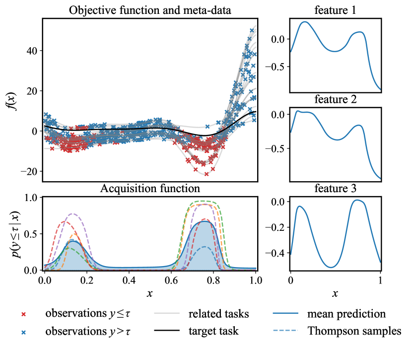
Figure 1: Illustration of meta-learning the acquisition function. Left: The top panel shows observations from 10 related tasks and the target task. The top performing observations ($\tau=\phi^{-1}(\gamma),\gamma=1/3$) in each task are shown in red, the rest in blue. The bottom panel shows the maximum-a-posteriori estimate of the acquisition function in solid while the Thompson samples are shown in dashed curves. Right: Features learned by our model, showing that MALIBO successfully identifies the promising areas, while the Thompson samples show variability in the meta-learned acquisition function.

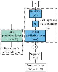
Figure 2: Schematic representation of our meta-learning classifier. A Residual Feedfoward Network (ResFFN) maps the input $\mathbf{x}$ via a shared feature mapping function $\phi$. From this, we construct a task-agnostic mean prediction $m(\bm{\Phi})$ and task-specific embedding $\mathbf{z}_{t}$, which is distributed according to a prior distribution $p(\mathcal{Z})$. The feature mapping function $\phi$ and mean prediction $m$ are fixed after meta-training, denoted by the task-agnostic component $g_{\bm{\omega}}$. Finally, we add and convert them to a class prediction.

Network structure

MALIBO uses a structured neural network that combines a meta-learned task-agnostic model with task-specific layer. We show an overview in Figure 2 and provide details for the choices below. Following previous works [5, 46], our meta-learning model uses a deterministic, task-agnostic model to map the input into features $\bm{\Phi}=\phi(\mathbf{x})$, where $\phi:\mathcal{X}\rightarrow\mathbb{R}^{d}$ is a learnable feature mapping shared across all tasks and $d$ is the predefined dimensionality of the feature space. We use a Residual Feedforward Network (ResFFN) for learning $\phi$, which has been shown to be robust to network hyperparameters and generalizes well to different problems [30]. To enable our model to provide good initial proposals, we introduce a task-agnostic mean prediction layer $m:\mathbb{R}^{d}\rightarrow\mathbb{R}$ that learns the promising areas from the related tasks. We refer to the combined task-agnostic components $m$ and $\phi$ as $g_{\bm{\omega}}$ (shown in blue), which is parameterized by $\bm{\omega}$. To allow adaptation on each task $t$, we use a task prediction layer $r_{t}:\mathbb{R}^{d}\rightarrow\mathbb{R}$, which is parameterized by layer weights $\mathbf{z}_{t}\in\mathcal{Z}\subseteq\mathbb{R}^{d}$. Since each $\mathbf{z}_{t}$ embeds in a low dimensional latent space $\mathcal{Z}$ and is a unique vector for each task, we refer to $\mathbf{z}_{t}$ as the task-specific embedding and to $\{\mathbf{z}_{t}\}$ as the set of embeddings for all meta-tasks. We will train our model such that the $\{\mathbf{z}_{t}\}$ follow a known distribution $p(\mathcal{Z})$ and discuss below how to use this as a prior for target task adaptation. Lastly, in order to obtain classification outputs as in LFBO, we apply logistic regression subsequently to produce probabilistic class predictions $p(k=1\mid\mathbf{x})$. The prediction for an observation in task $t$ is then given by $C(\mathbf{x}_{t})=\sigma(m(\bm{\Phi})+\mathbf{z}_{t}^{\mathsf{T}}\bm{\Phi})$.

Meta-learning

Directly optimizing $\mathcal{L}^{\text{{LFBO}}}$ to meta-learn our model would lead to task embeddings that do not conform to any particular prior task distribution $p(\mathcal{Z})$, and thus render task adaptation difficult and unreliable [19]. Therefore, we regularize the task embeddings $\{\mathbf{z}_{t}\}$ during training to enable Bayesian inference. In addition, such regularization can also avoid overfitting in the task space $\mathcal{Z}$ and improves the generalization performance of our model. Specifically, we assume the prior of the task embeddings to be a multivariate normal (MVN), $p(\mathcal{Z})=\mathcal{N}(\mathbf{0},\mathbf{I})$ and apply a regularization term to bring the empirical distribution of the $\{\mathbf{z}_{t}\}$ close to the prior distribution. The loss used for training on the meta-data reads:

$$\mathcal{L}^{\text{meta}}(\bm{\omega},\{\mathbf{z}_{t}\}_{t=1}^{T})=\frac{1}{T}\sum_{t=1}^{T}\mathcal{L}^{\textsc{LFBO}}(\bm{\omega},\mathbf{z}_{t};\mathcal{D}^{t},\tau)+\lambda\mathcal{R}(\{\mathbf{z}_{t}\}_{t=1}^{T};p(\mathcal{Z}))\,,$$ (3)

where the first term is the loss function from LFBO as in Equation 2, weighting the observations in the meta-data with improvements and the second term $\mathcal{R}$ is the regularization term weighted by $\lambda$. We regularizes the empirical distribution of $\{\mathbf{z}_{t}\}$ to match the Gaussian prior in a tractable way [52, 5]:

$$\mathcal{R}(\{\mathbf{z}_{t}\}_{t=1}^{T};p(\mathcal{Z}))=\lambda_{\text{KS}}\sum^{d}_{j=1}(F([\mathbf{z}_{t}]_{j})-\Phi([\mathbf{z}_{t}]_{j}))^{2}+\lambda_{\text{Cov}}\|\mathbf{I}-\text{Cov}(\{\mathbf{z}_{1},\dots,\mathbf{z}_{T}\})\|^{2}_{\mathrm{F}}\,,$$ (4)

where the first term matches the marginal CDFs similar to a Kolmogrov-Smirnov (KS) test, and the second term matches the empirical covariance of the task embeddings to the covariance of the prior. The hyperparameters $\lambda_{\text{KS}}$ and $\lambda_{\text{Cov}}$ encode the trade-off between these two terms. We denote $F$ as the empirical CDF and Cov as the empirical covariance matrix. For more details we refer to Appendix C.

We only consider a uni-modal Gaussian prior in this work, as we will show it already demonstrates strong performance against other baselines. For more complex task distributions, one could extend it with multi-modal Gaussian prior [52].

Task adaptation

After meta-training, the model can efficiently adapt to new tasks by estimating an embedding $\mathbf{z}$ based on the learned feature mapping function $\phi$. In principle, one could use a maximum likelihood classifier obtained by directly optimizing Equation 2 w.r.t. $\mathbf{z}$. However, such a classifier does not consider the task uncertainty and would suffer from unreliable adaptation [19] and over-exploitation [61, 56, 44]. Furthermore, when a potential disparity between the distribution of the meta-data and the non-i.i.d. data collected during optimization arises, a probabilistic model would be informed via uncertainty estimation and thereby can exploit less knowledge learned from the meta-data. Therefore, we propose to use a Bayesian approach for task adaptation, which makes our classifier uncertainty-aware and more exploratory.

Consider the task embedding $\mathbf{z}$ for the target task follows a distribution $p(\mathbf{z}\mid\mathcal{D}_{N})$ after $N$ observations, then the predictive distribution of our model can be written as

$$C(\mathbf{x};\bm{\omega},\mathcal{D}_{N})=\int p(k=1\mid\bm{\omega},\mathbf{z})p(\mathbf{z}\mid\mathcal{D}_{N})\,\mathrm{d}\mathbf{z}\,,$$ (5)

which accounts for the epistemic uncertainty in the task embedding. Since the parameters $\bm{\omega}$ of task-agnostic model $g_{\bm{\omega}}$ are fixed after meta-training, we denote our classifier as $C(\mathbf{x})$ for simplicity.

As there is no analytical way to evaluate the integration in Equation 5, we have to resort to approximation methods, such as variational inference [25, 7], Laplace approximation [6, 41], and Markov chain Monte Carlo [42, 29]. We consider the Laplace approximation for the task posterior distribution $p(\mathbf{z}\mid\mathcal{D}_{N})$ as a fast and scalable method, and show its competitive performance against other more expensive alternatives in Section E.3.

The Laplace’s method aims to fit a Gaussian distribution around the maximum-a-posteriori (MAP) estimate of the distribution and match the second order derivative at the optimum. In the first step, we obtain the MAP estimate by maximizing the posterior of our classifier $C$ parameterized by $\mathbf{z}$. To be consistent with the regularization used during meta-training, we use a standard, isotropic Gaussian prior for the weights: $p(\mathbf{z})=\mathcal{N}(\mathbf{z}\mid\mathbf{0},\mathbf{I})$. Given observations $\mathcal{D}_{N}$, the negative log posterior $p(\mathbf{z}\mid\mathcal{D}_{N})$ is proportional to

$$\mathcal{L}^{\textsc{MALIBO}}(\mathbf{z})=\frac{1}{2}\mathbf{z}^{\mathsf{T}}\mathbf{z}-\sum^{N}_{n=1}\left(k_{n}(\tau-y)\ln\hat{k}_{n}+\ln(1-\hat{k}_{n})\right)\,,$$ (6)

where $\hat{k}=\sigma(m(\bm{\Phi})+\mathbf{z}^{\mathsf{T}}\bm{\Phi})$ is the class probability prediction and the MAP estimate of the weights given by $\mathbf{z}_{\text{MAP}}={\arg\min}_{\mathbf{z}\in\mathcal{Z}}\mathcal{L}^{\textsc{MALIBO}}$. As a second step, we compute the negative Hessian of the log posterior

$$\mathbf{\Sigma}_{N}^{-1}=\nabla\nabla\mathcal{L}^{\text{{MALIBO}}}=\mathbf{\Sigma}_{0}^{-1}+\sum_{n=1}^{N}(k_{n}(\tau-y)+1)\hat{k}_{n}(1-\hat{k}_{n})\bm{\Phi}_{n}\bm{\Phi}_{n}^{\mathsf{T}}\,,$$ (7)

which serves as the precision matrix for the approximated posterior $q(\mathbf{z})=\mathcal{N}(\mathbf{z}\mid\mathbf{z}_{\text{MAP}},\mathbf{\Sigma}_{N})$. Therefore Equation 5 can be approximated as

$$C(\mathbf{x})\simeq\int p(k=1\mid\bm{\omega},\mathbf{z})q(\mathbf{z})\,\mathrm{d}\mathbf{z}\,.$$ (8)

Uncertainty-based exploration

During early phase in optimization, every meta-learning model has to reason about the target task properties based only on limited data that are available, which can lead to highly biased results and over-exploitation [19]. Moreover, it is shown that LFBO also suffer from similar issue even without meta-learning [61, 56, 44]. Therefore, we propose to use Thompson sampling based on task uncertainty for constructing a more exploratory acquisition function, and the resulting sampled predictions is generated by

$$\hat{C}(\mathbf{x})=\sigma\left(m(\bm{\Phi})+\hat{\mathbf{z}}^{\mathsf{T}}\bm{\Phi})\right),\quad\hat{\mathbf{z}}\sim q(\mathbf{z})\,.$$ (9)

Besides stronger exploration in the early phases of optimization, Thompson sampling also enables us to extend MALIBO to parallel BO by using multiple Thompson samples of the acquisition function in parallel. It is shown that this bypasses the sequential scheme of traditional BO, without introducing the common computational burden of more sophisticated methods [32]. We believe this to be a valuable strategy for parallelization and briefly explore it in Appendix F.

Gradient boosting as a residual prediction model

Operating in a meta-learned feature space enables fast task adaptation for our Bayesian classifier. However, it relies on the assumption that the meta-data is sufficient and representative for the task distribution , which does not always hold in practice. Moreover, a distribution mismatch between observations $\mathcal{D}_{N}$ and meta-data $\mathcal{D}^{\text{meta}}$ can arise when $\mathcal{D}_{N}$ is generated by an optimization process while $\mathcal{D}^{\text{meta}}$ consists of, e.g., i.i.d. samples.

We employ a residual model independent of the meta-learning model, such that, even given non-informative features, our classifier is able to regress to an optimizer that operates in the input space $\mathcal{X}$. We propose to use gradient boosting (GB) [22] as a residual prediction model for classification, which consists of an ensemble of weak learners that are sequentially trained to correct the errors from the previous ones. Specifically, we replace the first weak learner by a strong learner, namely, our meta-learned classifier. With Thompson sampling, our classifier can be written as

$$C_{\text{GB}}(\mathbf{x})=\sigma\left(m(\bm{\Phi})+\hat{\mathbf{z}}^{\mathsf{T}}\bm{\Phi}+\sum^{M}_{i=1}h_{i}(\mathbf{x})\right)\,,$$ (10)

where each $h_{i}$ represents the $i$-th trained base-learner for the error correction from gradient boosting. In addition to robust task adaptation, this approach offers two advantages: First, gradient boosting does not require an additional weighting scheme for combining different classifiers and automatically determines the weight of the meta-learned model; Second, gradient boosting demonstrates strong performance for LFBO on various benchmark [56], making our classifier remain competitive performance even when meta-learning fails as shown in Section E.2.

The resulting residual model is trained solely on data collected during optimization, and thus might overfit in the early iterations with limited data. To avoid this, we apply gradient boosting only after a few iterations of Thompson sampling exploration and train it with early stopping. Note that this does not diminish the usefulness of the residual model, because our goal is to encourage exploration in early iterations as outlined in Section 4, and gradually rely more on the knowledge from the target task once sufficiently many observations have been obtained. We refer to Appendix H for details.

Meta-learning:

Input: $\mathcal{D}^{\text{meta}}=\{\mathcal{D}^{t}\}_{t=0}^{T}$ , proportion $\gamma\in(0,1)$

1

2 $k=\mathbbm{1}(y\leq\tau)$, where $\tau=\Phi^{-1}(\gamma)$

3  // generate binary labels

4

5$g_{\bm{\omega}}\leftarrow\operatorname*{arg\,min}_{\bm{\omega}}\mathcal{L}^{\text{meta}}\qquad\qquad$

6  // train meta-model $g_{\bm{\omega}}$, Equation 3

7

Bayesian optimization with Meta-learning:

Input: Fixed $g_{\bm{\omega}}$ after meta-leaning

8

9 $\mathbf{x}_{0}\leftarrow\operatorname*{arg\,max}_{\mathbf{x}}g_{\bm{\omega}}(\mathbf{x})$  $\mathcal{D}\leftarrow\{(\mathbf{x}_{0},f(\bm{x}_{0})+\epsilon)\}$ 

10while has budget do

11      $\mathbf{z}_{\text{MAP}}\leftarrow\operatorname*{arg\,min}_{\mathbf{z}}\mathcal{L}^{\textsc{MALIBO}}$

12       // Equation 6

13     

14     Update precision matrix $\mathbf{\Sigma}_{n}^{-1}$

15       // Equation 7

16     

17     $\hat{\mathbf{z}}\sim\text{MVN}(\mathbf{z}_{\text{MAP}},\mathbf{\Sigma}_{N})$

18     

19     $\mathbf{x}_{*}\leftarrow\arg\max_{\mathbf{x}}C_{\text{GB}}(\mathbf{x};{\hat{\mathbf{z}}})$

20       // Equation 10

21     

22     $\mathcal{D}\leftarrow\mathcal{D}\cup\{(\mathbf{x}_{*},f(\mathbf{x}_{*})+\epsilon)\}$ 

Algorithm 1 MALIBO: Meta-learning for likelihood-free Bayesian optimization

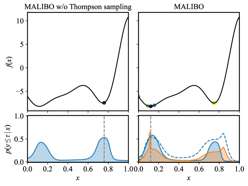
Figure 3: Effects of Thompson sampling and residual prediction on optimizing a Forrester function. Color circles denote the optimization queries (from bright to dark), dashed curve denotes a Thompson sample of the acquisition function and the orange curve shows the sample combined with gradient boosting.

5 Experiments

In this section, we first show a preliminary ablation study to exhibit the effect of using Thompson sampling and gradient boosting. We then describe the experiments conducted to empirically evaluate our method. For the choice of problems, we focus on automated machine learning (AutoML), i. e. hyperparameter optimization (HPO) and neural architecture search (NAS). To study robustness towards data with heterogeneous scale and noise, we evaluate our method on synthetic functions with multiplicative noise. We show that MALIBO outperforms other state-of-the-art meta-learning BO methods in AutoML problems and is robust to heterogeneous scale and noise.

Baselines

We compare our method against state-of-the-art baselines across all problems. As methods without meta-learning, we picked random search [3], LFBO [56] and GP-UCB [58] for our experiments. For meta-learning BO methods, we chose ABLR [46], RGPE [16], GC3P [50] and MetaBO [65] as representative algorithms. Additionally, we consider a simple baseline for extending LFBO with meta-learning, called LFBO+BB, which combines LFBO with bounding-box search space pruning [47] as a meta-learning approach. For all LFBO-based methods, including MALIBO, we set the required threshold hyperparameter $\gamma=1/3$ following [61, 56].

Evaluation metrics

In order to aggregate performances across tasks, we use normalized regret as the quantitative performance measure for AutoML problems [72, 50]. This is defined as $\min_{\mathbf{x}\in\mathcal{X}_{n}}(f^{t}(\mathbf{x})-f^{t}_{\text{min}})/(f^{t}_{\text{max}}-f^{t}_{\text{min}})$, where $\mathcal{X}_{n}$ denotes the set of inputs that have been selected by an optimizer up to iteration $n$, $f^{t}_{\text{min}}$ and $f^{t}_{\text{max}}$ respectively represent the minimum and the maximum objective computed across all offline evaluations available for task $t$. We report the mean of normalized regrets across all tasks within a benchmark as the aggregated result. For all benchmarks, we report the results by mean and standard error across 100 random runs.

Effects of exploration and residual prediction

We first demonstrate the effect of Thompson sampling and the residual prediction model for optimizing a Forrester function [55] as a toy example. By using the meta-learned model as shown in Figure 2, MALIBO performs task adaptation for a new Forrester function for $10$ iterations. We compare the results of MALIBO against a variant without the proposed Thompson sampling and gradient boosting, which only uses the approximated posterior predictive distribution in Equation 8 by probit approximation [41] for the acquisition function. As shown in Figure 3, MALIBO without Thompson sampling fails to adapt the new task with little exploration and optimizes greedily around the local optimum. This greedy optimization occurs due to the strong dependence of LFBO on a good initialization to not over-exploit. In contrast, the proposed MALIBO allows the queries to cover both possible optima by encouraging explorations. In addition, gradient boosting performs the refinement beyond the smooth meta-learned acquisition function, which can be seen in the discontinuity in the predictions. By suppressing the predicted utility in the less promising areas, gradient boosting refines the acquisition function and shifts the proposed query to a lower value region.

Real-world benchmarks

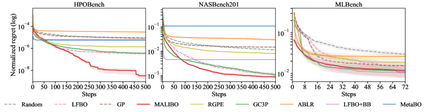
Figure 4: Aggregated normalized regrets for different BO algorithms on real-world AutoML problems.

We empirically evaluate our method on various real-world optimization tasks, focusing on AutoML problems, including neural architecture search (NASBench201 [12]), hyperparameter optimization for neural networks (HPOBench [35]) and machine learning algorithms (MLBench [14]).

In NASBench201, we consider designing a neural cell with $6$ discrete parameters, totaling $15,625$ unique architectures, evaluated on CIFAR-10, CIFAR-100 [36] and ImageNet-16 [9]. We aim to find the optimal architecture for a neural network that yields the highest validation accuracy. For HPOBench, we aim to find the optimal hyperparameters for a two-layer feed-forward regression network on four popular UCI datasets [13]. The search space is $9$-dimensional and the optimization objective is the validation mean squared error after training the corresponding network configuration. In MLBench, we picked $5$ algorithms (SVM, LogReg, XGBoost, RandomForest and MLP) from the ML benchmark suite [14]. They are evaluated on $20$ OpenML tasks [64], except for MLP with only 8 tasks (as defined in the benchmark). The search spaces dimensions range from $2$ (SVM) to $5$ (MLP) with the same objective as in NASBench201. We provide details for benchmarks in Appendix I.

To train and evaluate the meta-learning BO methods, we conduct our experiment in a leave-one-task-out way: all meta-learning methods use one task as the target task and all others as related tasks. In this way, every task in a benchmark has been picked as the target task once. To construct the meta-datasets for meta-learning, we randomly select $N$ configuration-objective pairs from the related tasks. For NASBench201 and HPOBench, we set $N$ to be $512$, while for MLBench, $N$ is $128$. All meta-learning methods, except MetaBO, are trained from scratch for each independent run, to account for variations due to the randomly sampled meta-data. Because of its long training time, MetaBO is trained once for each target problem on more meta-data than other methods to avoid limiting its performance with a bad subsample. We show its results only for HPOBench and NASBench201, and refer to Appendix H for details.

The aggregated results for all three benchmarks are summarized in Figure 4. It is evident that MALIBO consistently achieves strong anytime performance, surpassing other methods that either exhibit poor warm-starting or experience early saturation of performance. Notably, MALIBO outperforms other methods by a large margin in HPOBench, primarily because we focus on minimizing the validation error of a regression model in this benchmark. This task poses a significant challenge for GP-based regression models, as the observation values undergo abrupt changes and have varying scales across tasks, thereby violating the smoothness and noise assumptions inherent in these models. In all benchmarks, GC3P performs competitively only after the Copula process is fitted and LFBO matches its final performance. LFBO+BB exhibits similar performance as MALIBO in warm-starting and converges quickly, but the search space pruning technique forbids the method to explore regions beyond the promising areas in the meta-data, making its final performance even worse than its non-meta-learning counterpart. ABLR and RGPE performs poorly on most of the benchmarks, except for MLBench, because their meta-learning techniques require more meta-data for effective warm-starting, making them less data-efficient than MALIBO. MetaBO shows strong warm-starting performance in HPOBench while it fails in NASBench. This is because due to the fact that the tasks in NASBench are much more diverse than in HPOBench, and MetaBO fails to transfer knowledge from tasks that are different from the target task. Moreover, MetaBO adapts poorly to the task, as reported in other studies [70, 67]. For more experimental results, we refer to Appendix G.

Runtime analysis

To confirm the scalability of MALIBO, we compared its runtime against the baseline methods for different benchmarks. We observed that latent features and the Laplace approximation only introduces a negligible overhead compared to LFBO and MALIBO’s runtime grows slowly with the number of observations. All other meta-learning methods, except for LFBO+BB, are considerably slower than MALIBO. We show our detailed experimental results in Appendix D.

Robustness against heterogeneous noise

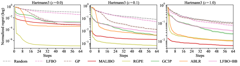
Figure 5: Normalized regret for different BO algorithms on Hartmann3 ensembles ($D=3$) with various levels of multiplicative noise.

We use synthetic function ensembles [5] to test the robustness against heterogeneous noise in the data. We focus on the Hartmann3 function ensemble [11], which is a three-dimensional problem with four local minima. Their location and the global minimum varies across different functions in the ensemble. See Appendix I for more details.

To avoid biasing this experiment towards a single method, we use a heteroscedastic noise incompatible with any assumptions about the noise of any method. In particular, this violates the GP methods’ and ABLR’s assumption of homoscedastic, Gaussian noise. GC3P makes a similar assumption after the nonlinear transformation of the observation values, which does not translate to any well-known noise model. LFBO, LFBO+BB and MALIBO make no explicit noise assumptions, but optimize for the best mean. We choose a multiplicative noise, i.e. $y=f(\mathbf{x})\cdot(1+\epsilon\cdot n)$, where $n\sim\mathcal{N}(\mathbf{0},\mathbf{1})$. The noise corrupts observations with larger values more, while having a smaller effect on those with lower values. To see the robustness with different noise levels, we evaluate $\epsilon\in\{0,0.1,1.0\}$. For meta-training, we randomly sampled $512$ noisy observations from $256$ functions in the ensemble. We show our results in Figure 5, where we can see across all noise levels, our method learns a meaningful prior for the optimization. The GP-based methods, despite their strong performance in the noise-free case, especially RGPE, degrade significantly with increasing noise levels.

6 Conclusion

We introduced MetA-learning for LIkelihood-free BO (MALIBO), which models the acquisition function directly from observations coupled with meta-learning. The method is computationally efficient and robust to heterogeneous scale and noise in the meta-data, which is challenging for other methods. In addition to the improved data efficiency, MALIBO uses a Bayesian classifier with Thompson sampling to account for task uncertainty, enabling our model to adapt to the tasks reliably. To ensure robust adaption to tasks that are not captured by the meta-learning, we incorporate gradient boosting into our model. Empirical results demonstrate superior performance on real-world benchmarks, as well as synthetic benchmarks with heteroscedastic noise.

Despite the promising experimental results, some limitations of the method should be noted. (i) The exploitation and exploration parameter $\tau$ in likelihood-free BO algorithms could be treated more carefully, e.g. via a probabilistic treatment [61]. (ii) The value of the regularization hyperparameter $\lambda$ used throughout all experiments seems robust, but could lead to sub-optimal behavior on other problems. (iii) For more complex task distribution, our uni-modal prior could become a limiting factor. While the GMM generalization of exists [52], there is no guarantee for its performance within MALIBO.

Supplementary Material

In the appendix we provide additional details on our method, ablation studies, additional results and experiments.

Appendix A Likelihood-free acquisition functions

For completeness, we provide the proofs and derivations for TPE [4], BORE [61], and LFBO [56]. Recall from Equation 1 that the expected utility function is defined as the expectation of the improvement of the utility function $U(y;\tau)$ over the posterior predictive distribution. Given $N$ observations on the target task in a non-meta-learning setting, for the specific expected improvement (EI) acquisition function, where the utility function is $U(y;\tau):=\max(\tau-y,0)$, the function reads:

$$\begin{split}\alpha^{U}(\mathbf{x};\mathcal{D}_{N},\tau)=\mathbb{E}_{p(y\mid\mathbf{x},\mathcal{D}_{N})}[U(y;\tau)]&=\int_{-\infty}^{\infty}U(y;\tau)p(y\mid\mathbf{x},\mathcal{D}_{N})\,\mathrm{d}y\\ &=\int_{-\infty}^{\tau}(\tau-y)p(y\mid\mathbf{x},\mathcal{D}_{N})\,\mathrm{d}y\\ &=\frac{1}{p(\mathbf{x}\mid\mathcal{D}_{N})}\int_{-\infty}^{\tau}(\tau-y)p(\mathbf{x}\mid y,\mathcal{D}_{N})p(y\mid\mathcal{D}_{N})\,\mathrm{d}y\,.\end{split}$$ (11)

We follow the prove from Tiao et al. [61] and consider $\ell(\mathbf{x})=p(\mathbf{x}\mid y\leq\tau,\mathcal{D}_{N})$ and $g(\mathbf{x})=p(\mathbf{x}\mid y>\tau,\mathcal{D}_{N})$. The denominator of the above equation can then be written as:

$$\begin{split}p(\mathbf{x}\mid\mathcal{D}_{N})&=\int_{-\infty}^{\infty}p(\mathbf{x}\mid y,\mathcal{D}_{N})p(y\mid\mathcal{D}_{N})\,\mathrm{d}y\\ &=\ell(\mathbf{x})\int_{-\infty}^{\tau}p(y\mid\mathcal{D}_{N})\,\mathrm{d}y+g(\mathbf{x})\int_{\tau}^{\infty}p(y\mid\mathcal{D}_{N})\,\mathrm{d}y\\ &=\gamma\ell(\mathbf{x})+(1-\gamma)g(\mathbf{x})\,,\end{split}$$ (12)

where $\gamma=\Phi(\tau)\coloneqq p(y\leq\tau\mid\mathcal{D}_{N})$. The numerator can be evaluated as:

$$\int^{\tau}_{-\infty}(\tau-y)p(\mathbf{x}\mid y,\mathcal{D}_{N})p(y\mid\mathcal{D}_{N})\,\mathrm{d}y =\ell(\mathbf{x})\int^{\tau}_{-\infty}(\tau-y)p(y\mid\mathcal{D}_{N})\,\mathrm{d}y$$ (13)

$$=\ell(\mathbf{x})\tau\int^{\tau}_{-\infty}p(y\mid\mathcal{D}_{N})\,\mathrm{d}y-\ell(\mathbf{x})\int^{\tau}_{-\infty}yp(y\mid\mathcal{D}_{N})\,\mathrm{d}y$$ (14)

$$=\gamma\tau\ell(\mathbf{x})-\ell(\mathbf{x})\int^{\tau}_{-\infty}yp(y\mid\mathcal{D}_{N})\,\mathrm{d}y$$ (15)

$$=K\cdot\ell(\mathbf{x})\,,$$ (16)

where $K=\gamma\tau-\int^{\tau}_{-\infty}yp(y\mid\mathcal{D}_{N})\,\mathrm{d}y$. Therefore the EI acquisition function is equivalent to the $\gamma$-relative density ratio up to a constant $K$,

$$\underbrace{\alpha(\mathbf{x};\mathcal{D}_{N},\tau)}_{\text{expected improvement}}\propto\underbrace{\frac{\ell(\mathbf{x})}{\gamma\ell(\mathbf{x})+(1-\gamma)g(\mathbf{x})}}_{\gamma-\text{relative density ratio}}$$ (17)

Intuitively, one can think of the configurations $\mathbf{x}$ with $y\leq\tau$ as good configurations, and the those with $y>\tau$ as bad configurations. Then the density ratio can be interpreted as the ratio between the model’s prediction whether the configurations belong to the good or bad class.

The tree-structured Parzen estimator (TPE) [4] estimates this density ratio by explicitly modeling $\ell(\mathbf{x})$ and $g(\mathbf{x})$ using kernel density estimation for a fixed value of the hyperparameter $\gamma$. Within BORE [61], the density ratio is modeled by class probabilities, where $\ell(\mathbf{x})=p(\mathbf{x}\mid y\leq\tau,\mathcal{D}_{N})$ and $g=p(\mathbf{x}\mid y>0,\mathcal{D}_{N})$.

Song et al. [56] proof that the density ratio acquisition functions are not always equivalent to EI. Bergstra et al. [4] and Tiao et al. [61] claim that Equation 13 holds true by assuming $\ell(\mathbf{x})$ is independent of $y$ once $y\leq\tau$ and therefore can be treated as a constant inside the integral. In reality, $p(\mathbf{x}\mid y\leq\tau,\mathcal{D}_{N})$ still depends on $y$ even if $y\leq\tau$, because it is a conditional probability conditioned on $y$ not $y\leq\tau$. Therefore, satisfying the condition $y\leq\tau$ does not imply independence of $y$. From the definition of conditional probability

$$p(\mathbf{x}\mid y\leq\tau,\mathcal{D}_{N})=\frac{\int_{-\infty}^{\tau}p(\mathbf{x},y\mid\mathcal{D}_{N})\,\mathrm{d}y}{\int_{-\infty}^{\tau}p(y\mid\mathcal{D}_{N})\,\mathrm{d}y}\neq p(\mathbf{x}\mid y,\mathcal{D}_{N})\,,$$ (18)

we can see that they are not equivalent. Intuitively, the probability of the configuration $\mathbf{x}$ for a given $y$ value should still depend on $y$ even if $y<\tau$ holds. By making this independence assumption, the resulting density ratio acquisition function treats all $(\mathbf{x},y)$ pairs below the threshold with equal probability (importance), when, in fact, EI weights the importance of $(\mathbf{x},y)$ pairs by the utility $\max(\tau-y,0)$

To tackle this issue, Song et al. [56] propose to directly approximate EI inspired by the idea of variational f-divergence estimation [43]. They provide a variational representation for the expected utility function at any point $\mathbf{x}$, provided samples from $p(y\mid\mathbf{x})$. Thereby, their approach replaces the potentially intractable integration with the variational objective function that can be solved based on samples:

$$\mathbb{E}_{p(y\mid\mathbf{x})}[U(y;\tau)]=\operatorname*{arg\,max}_{s\in[0,\infty)}\mathbb{E}_{p(y\mid\mathbf{x})}[U(y;\tau)f^{\prime}(s)]-f^{\star}(f^{\prime}(s))\,,$$ (19)

where the utility function $U:\mathbb{R}\times\mathcal{T}\rightarrow[0,\infty)$ is non-negative, $\tau\in\mathcal{T}$, $f:[0,\infty)\rightarrow\mathbb{R}$ is a strictly convex function with third order derivatives, and $f^{\star}$ is the convex conjugate of $f$. The maximization is performed over $s\in[0,\infty)$ and it does not model distributions with probability but only samples from the observations $\mathcal{D}_{N}$.

They consider the approximated expected utility acquisition function as $\alpha^{\textsc{LFBO}}=\hat{S}_{\mathcal{D}_{N,\tau}}(\mathbf{x})$, which can be written as:

$$\hat{S}_{\mathcal{D}_{N,\tau}}(\mathbf{x})=\operatorname*{arg\,max}_{S:\mathcal{X}\rightarrow\mathbb{R}}\mathbb{E}_{\mathcal{D}_{N}}[U(y;\tau)f^{\prime}(S(\mathbf{x}))-f^{\star}(f^{\prime}(S(\mathbf{x}))].$$ (20)

By optimizing a variational objective in the search space $\mathcal{X}$, the expected utility acquisition function over $\mathbf{x}$ can be recovered. For practical purpose, they choose a specific convex funciton $f$: $f(r)=r\log\frac{r}{r+1}+\log\frac{1}{r+1}$ for all $r>0$, and a specific form of $S=C/(1-C)$, where $C:\mathcal{X}\rightarrow(0,1)$ and can be considered as a probabilistic classifier. By applying these into Equation 20, the resulting acquisition function reads:

$$\alpha^{\text{LFBO}}(\mathbf{x};\mathcal{D}_{N},\tau)=\hat{S}_{\mathcal{D}_{N},\tau}(\mathbf{x})=\hat{C}_{\mathcal{D}_{N},\tau}(\mathbf{x})/(1-\hat{C}_{\mathcal{D}_{N},\tau}(\mathbf{x})),$$ (21)

where $\hat{C}_{\mathcal{D}_{N},\tau}$ is the maximizer of an objective over $C$:

$$\mathbb{E}_{(\mathbf{x},y)\sim\mathcal{D}_{N}}[U(y;\tau)\ln C(\mathbf{x})+\ln(1-C(\mathbf{x}))]\,.$$ (22)

This is can be reinterpreted as a classification loss with training examples weighted by the utility function.

Appendix B Probit approximation

Let $a=m(\bm{\Phi})+\mathbf{z}^{\mathsf{T}}\bm{\Phi}$ and $q(\mathbf{z})=\mathcal{N}(\mathbf{z}\mid\mathbf{z}_{\text{MAP}},\mathbf{\Sigma}_{N})$ be the approximated posterior obtained through the Laplace approximation. The distribution of $a$ then follows the Gaussian $\mathcal{N}(a\mid\mu_{a},\sigma_{a}^{2})$ with the following parameters:

$$\mu_{a}=\mathbb{E}[a]=\int p(a)a\,da=\int q(\mathbf{z})(m(\bm{\Phi})+\mathbf{z}^{\mathsf{T}}\bm{\Phi})\,d\mathbf{z}=m(\bm{\Phi})+\mathbf{z}_{\text{MAP}}^{\mathsf{T}}\bm{\Phi}\,,$$ (23)

$$\begin{split}\sigma_{a}^{2}&=\int p(a)[a^{2}-\mathbb{E}[a]^{2}]\,\mathrm{d}a\\ &=\int q(\mathbf{z})\left((m(\bm{\Phi})+\mathbf{z}^{\mathsf{T}}\bm{\Phi})^{2}-(m(\bm{\Phi})+\mathbf{z}_{\text{MAP}}^{\mathsf{T}}\bm{\Phi})^{2}\right)\,\mathrm{d}\mathbf{z}\\ &=\bm{\Phi}^{\mathsf{T}}\mathbf{\Sigma}_{N}\bm{\Phi}\,.\end{split}$$ (24)

Thus our approximation to the predictive distribution in Equation 8 becomes

$$C(\mathbf{x})\simeq\int p(k=1\mid\bm{\omega},\mathbf{z})q(\mathbf{z})\,\mathrm{d}\mathbf{z}=\int\sigma(a)\mathcal{N}(a\mid\mu_{a},\sigma_{a}^{2})\,\mathrm{d}a\,.$$ (25)

Since the integral in Equation 25 cannot be evaluated analytically due to the sigmoid function, we need to approximate it to obtain the marginal class prediction. One can approximate the integral by exploiting the similarity between the logistic sigmoid function $\sigma(a)$ and the inverse probit function [6, 41], which is given by the cumulative distribution of the standard Gaussian $\Phi(a)$. In order to obtain good approximation results, we need to rescale the horizontal axis so that $\sigma(a)$ has the same slope as $\Phi(\lambda a)$, where $\lambda^{2}=\pi/8$. By replacing $\sigma(a)$ with $\Phi(\lambda a)$ in Equation 25, we obtain the approximated predictive distribution:

$$\begin{split}p(k=1\mid\bm{\omega},\mathcal{D}_{N})&\approx\int\Phi(\lambda a)\mathcal{N}(a\mid\mu_{a},\sigma_{a}^{2})\,\mathrm{d}a\\ &=\Phi\left(\frac{\mu_{a}}{(\lambda^{-2}+\sigma_{a}^{2})^{1/2}}\right)\\ &=\sigma\left((1+\pi\sigma_{a}^{2}/8)^{-1/2}\mu_{a}\right)\,.\end{split}$$ (26)

Appendix C Regularizing the latent task space

To make sure our task distribution conforms to the prior distribution $p(\mathcal{Z})$, we followed the approach in Saseendran et al. [52] and Berkenkamp et al. [5], where they regularize the learned latent representation towards a given prior distribution in a tractable way. Their approach builds on the non-parameteric Kolmogorov-Smirnov (KS) test for one-dimension probability distributions and extend it to a multivariate setting, which allows for gradient-based optimization and can be easily applied to expressive multi-modal prior distributions.

Directly extending the KS test to high-dimensional distributions is challenging, since it requires matching joint CDFs, which is especially infeasible in this case. Therefore, they propose to match the marginal CDFs of the prior, making the regularization tractable. Given $d$-dimensional task embedding $\mathbf{z}_{1},\dots,\mathbf{z}_{T}$ for $T$ related tasks, the empirical CDF in dimension $j$ is defined as:

$$F(z)=\frac{1}{T}\sum^{T}_{t=1}\mathbbm{1}([\mathbf{z}_{t}]_{j}\leq z)\,,$$ (27)

where $\mathbbm{1}([\mathbf{z}_{t}]_{j}\leq z)$ is a indicator function if $j$-th component of $\mathbf{z}_{t}$ is smaller or equal than a certain value $z$. In addition to the marginals, they also regularize the empirical covariance matrix $\text{Cov}({\mathbf{z}_{1},\dots,\mathbf{z}_{T}})$ to be close to the covariance of the prior. In our case, the prior task distribution is a isotropic Gaussian $p(\mathcal{Z})=\mathcal{N}(\mathbf{0},\mathbf{I})$, and the resulting regularizer can be written as:

$$\mathcal{R}(\{\mathbf{z}_{t}\}_{t=1}^{T};p(\mathcal{Z}))=\lambda_{\text{KS}}\underbrace{\sum^{d}_{j=1}(F([\mathbf{z}_{t}]_{j})-\Phi([\mathbf{z}_{t}]_{j}))^{2}}_{\text{match marginal CDF of }p(\mathcal{Z)}}+\underbrace{\vphantom{\sum^{d}_{j=1}}\lambda_{\text{Cov}}\|\mathbf{I}-\text{Cov}(\{\mathbf{z}_{1},\dots,\mathbf{z}_{T}\})\|^{2}_{\mathrm{F}}}_{\text{match covariance of }p(\mathcal{Z})}\,,$$ (28)

where the marginal CDFs and correlations are compared through squared errors, the $\lambda_{\text{KS}}$ and $\lambda_{\text{CV}}$ are weighting factors controls the trade-off between matching the empirical marginal CDFs and the covariance.

Regularization coefficients estimation

The two regularization coefficients $\lambda_{\text{KS}}$ and $\lambda_{\text{Cov}}$ are important hyperparameters and needed to be carefully treated. Notice that, the more tasks we have, the closer the match between the empirical CDFs and the prior marginal CDF based on the assumption that the related tasks are i.i.d. samples from the task distribution. To avoid the regularization being dominated by one term, we aim to scale them in a way that all terms converge to similar magnitudes with more tasks. Therefore, we choose the two factors such that

$$\begin{split}\lambda_{\text{KS}}^{-1}&=2\sum^{d}_{j=1}(F([\mathbf{z}_{t}]_{j})-\Phi([\mathbf{z}_{t}]_{j}))^{2}\,,\qquad\text{with}\quad\mathbf{z}_{t}\sim p(\mathcal{Z})\,,\\ \lambda_{\text{Cov}}^{-1}&=2\|\mathbf{I}-\text{Cov}(\{\mathbf{z}_{1},\dots,\mathbf{z}_{T}\})\|^{2}_{\mathrm{F}}\,,\qquad\text{with}\quad\mathbf{z}_{t}\sim p(\mathcal{Z})\,,\end{split}$$ (29)

where $\mathbf{z}_{t}$ is i.i.d. sample from the prior distribution for the cofficient estimation. This normalizes the regularizer to be approximately of order $1$ for samples follows the prior distribution.

Appendix D Runtime analysis

The experiments in Section 5 show the performance over the optimization steps. To be complementary, we demonstrate the same results from a different perspective, namely, we report the normalized regrets as a function of the estimated wall-clock time. To obtain the realistic wall-clock time, we accumulate the time to optimize for corresponding BO methods and the recorded runtime for the configurations in the benchmarks. Notice that all the methods run for the same number of steps in an experiment.

The results in Figures 6, 7 and 8 show that MALIBO attains the best warm-starting performance across almost all benchmarks and constantly achieves one of the lowest final regrets in the same amount of time. While LFBO+BB starts the optimization with regrets close to MALIBO and even better on the NAS benchmarks, the performance saturates quickly. In contrast, LFBO starts with high regrets but shows competitive end performance. GC3P is the most consistent meta-learning baseline method with performance close to MALIBO in some of the benchmarks. However, the performance drops especially for NASBench201 and some of the MLBench problems, where the meta-learning fails to warm-start the optimization. Similarly, the meta-learning of RGPE and ABLR do not deliver consistent advantages over the baselines without meta-learning and often end up with regrets close to the GP based BO.

To further investigate the time efficiency of MALIBO, we illustrates the runtime of the optimization algorithms for each step in Figure 9. The runtime for MALIBO is the second fastest among all the meta-learning methods, while only slightly slower than LFBO and LFBO+BB. Due to the increasing amount of observations, the runtime of almost all the methods grows over with the number of iterations, especially for RGPE and GP, where the growths are the most significant. Although ABLR and GC3P are around one order of magnitude slower than MALIBO at the beginning, but their runtimes remain stable throughout the optimization. For ABLR this is to be expected for reasonably short runs, as the parametric model is always retrained on all data sets (including the target one) which constitutes the largest computational burden at each step and the complexity of the Bayesian linear regression scales more gracefully then the GPs. For GC3P, we attribute the almost constant runtime to very agressive settings for the GPs hyperparameter optimization, which is usually the most expensive step. By a smart intialization and good priors, Salinas et al. [50] were able to keep the runtime relatively constant for the shown number of steps. The growth in runtime for LFBO and LFBO+BB can be attributed exclusively to the fitting of the gradient boosted trees. Similarly, MALIBO uses gradient boosting as residual prediction model, which retrains on the dataset for every iteration, therefore the runtime grows with the number of iterations as well.

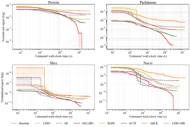
Figure 6: Normalized regrets of different BO algorithms on the HPOBench neural network tuning problem. Each algorithm runs for 500 iterations and we show the corresponding estimated wall-clock time on the $x$ axis in log scale.

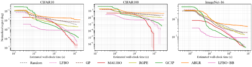
Figure 7: Normalized regrets of different BO algorithms on the NASBench201 neural network architecture search problem. Each algorithm runs for 200 iterations and we show the corresponding estimated wall-clock time on the $x$ axis in log scale.

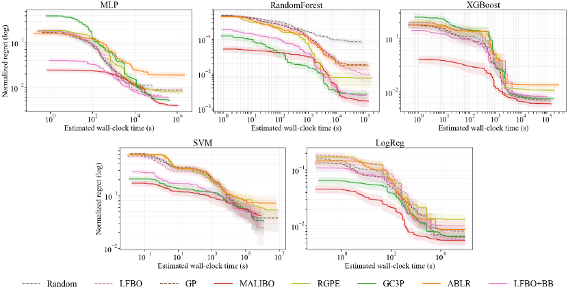
Figure 8: Normalized regrets of different BO algorithms on the HPOBench hyperparameter tuning for machine learning algorithms. Each algorithm runs for 72 iterations and we show the corresponding estimated wall-clock time on the $x$ axis in log scale.

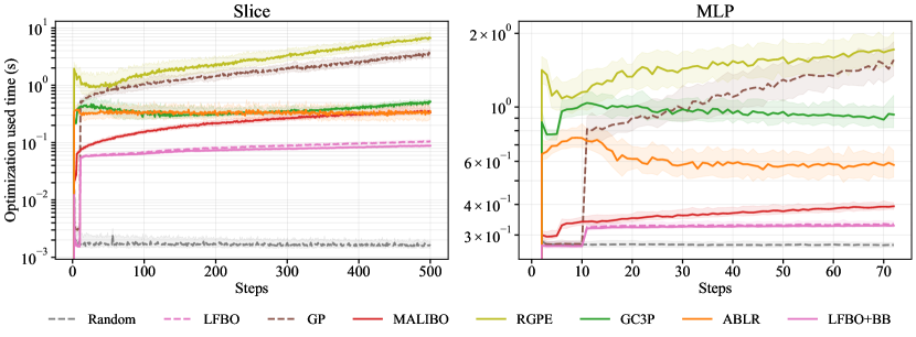
Figure 9: Runtime of different BO algorithms over optimization steps. We show the typical results for two benchmarks and plot the medial inter-quantiles to remove outliers.

Appendix E Ablation studies

We conduct ablation studies to show how the different components of MALIBO impact the optimization. To be specific, we first visualize the meta-learned feature representation for two different function in Section E.1 to provide some intuition for the expressiveness of our meta-learning model. To study the contribution of each component and how they benefit the optimization, we provide an ablation study in Section E.2 to demonstrate their usefulness. Lastly, we compared the performance of MALIBO using different inference methods in Section E.3.

E.1 Latent feature analysis

Here we visualize the feature representation extracted from the meta-data by our meta-learning model. The latent features $\mathbf{\Phi}$ represent basis functions for the Bayesian logistic regression and should represent the structure of the meta-data distribution. With successfully learned features $\mathbf{\Phi}$ and the mean layer, our model performs the task adaptation by reasoning about the latent task embedding vector $\mathbf{z}$. It produces predictions with similar structure to the meta-data that match the class labels on the target function.

In order to learn a effective feature representation, one should capture both the local and global structure of the function. Therefore, we select two types of function to study the effectiveness of feature learning for MALIBO: i) Forrester functions [55] with two very likely positions for the global optimum, which allows for effective warm-starting and requires local adaptation. ii) quadratic functions, where the functions share a certain global shape, but the optima could be located anywhere in the search space. For more details on the synthetic functions and the generation of meta-data, we refer to Appendix G.

The results for these two synthetic functions are shown in Figure 10(a) and Figure 10(b) respectively. On one hand, we can see that in Figure 10(a) the features learned by MALIBO have either a maximum or a minimum around the two likely optima, which means the model successfully infers the location of the most promising values from the meta-data. On the other hand, Figure 10(b) shows that, even without a clear location of optima, the features still follow the shape of quadratic functions with different minima.

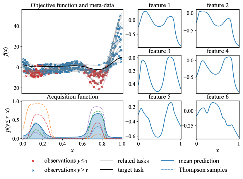
(a) Forrester function features

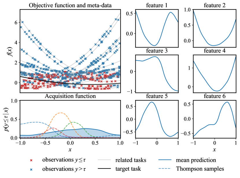
(b) Quadratic function features

Figure 10: Left: Forrester functions with two very likely optima as target function and related tasks. The learned acquisition function is shown below. The meta-learned latent features show that the model successfully infers the location of two optima, resulting in a acquisition with two modes around the optima. Right: Quadratic functions with varying optima as target function and related tasks. The meta-learned latent features show that the model is able to capture the global function shape shared across all the meta-data, even though there is no clear position for optima.

E.2 Effects of Thompson sampling and gradient boosting

MALIBO uses Bayesian logistic regression for task adaptation, which leverages the meta-learned feature. However, the performance depends heavily on the amount and quality of the data even with effectively learned latent features. For example, during early iterations of optimization, there are only limited data for the model to infer the characteristics of the target task, making the task ambiguous to the model. Moreover, the amount and the quality of meta-data are often not guaranteed in practice, e.g. the target task is too different from the meta-data. To tackle these limitations, we apply Thompson sampling as a exploratory strategy to account for task uncertainty, which enables MALIBO to collect more information about the target function by exploring the search space efficiently. Furthermore, we introduce gradient boosting as a residual model to safeguard the optimization when little meta-data or a large discrepancy between the training data and the meta-data distribution exists.

In this section, we first show how Thompson sampling affects the optimization process by encouraging exploration. Subsequently, we investigate the effect of adding gradient boosting as a residual model to guide the optimization to adapt to novel task. Finally, we compare experimental results with different variants of MALIBO, which show the superior performance of the proposed combination of Thompson sampling and gradient boosting over other possible variants.

Effects of Thompson Sampling

In order to show the exploration performance, we choose to compare the task adaptation performance among MALIBO (vanilla), MALIBO (TS) and MALIBO on synthetic benchmarks, where MALIBO (TS) only use Thompson sampling without gradient boosting and MALIBO (vanilla) uses the marginalized form of the acquisition function (see Appendix B) with no gradient boosting either.

As we can see in Figures 11 and 12, due to the lack of exploration, MALIBO (vanilla) exhibits conservative behavior in both Forrester and quadratic function which leads to suboptimal performance. With Thompson sampling, MALIBO (TS) demonstrates stronger exploration in both problems and is able to identify the area of global optimum quickly. Although MALIBO is equipped with gradient boosting, it shows similar exploration performance as the Thompson sampling only variant. The impact of gradient boosting is visible in the suppression of the acquisition function values in regions where the sampled function might predict high values, but a few observations indicate the opposite. It also increases the acquisition function values around the currently best observations which leads to stronger convergence.

In the early stage of the optimization, the task adaptation and gradient boosting do not have enough observations to have confident prediction. Unlike other methods, which use random search as a exploration strategy, Thompson sampling takes the task uncertainty into consideration and explores possible optima efficiently by reusing the meta-learned knowledge from related tasks.

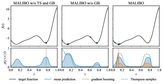
Figure 11: Task adaptation of different MALIBO variants on Forrester function after meta-learning. Each method optimize for $10$ iterations.

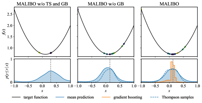
Figure 12: Task adaptation of different MALIBO variants on quadratic function after meta-learning. Each method optimize for $10$ iterations.

Effects of gradient boosting

To show the usefulness of gradient boosting in MALIBO, we remove the effects of meta-learning by optimizing the target synthetic functions without any meta-training, which simulates the situation when the meta-learning is not useful for task adaptation. Therefore the experiments will focus only on the effects on the gradient boosting and show how it can safeguard the optimization.

We first show the difference between different MALIBO variants on a Forrester function when no meta-learning is applied. In addition, we also show the optimization process for LFBO, as a comparison to MALIBO without meta-learning. As we can see in Figure 13, while MALIBO (vanilla) and MALIBO (TS) optimize the function inefficiently and fail to learn a model the acquisition function given the observations, MALIBO successfully identifies the optima and exhibits behavior comparable to LFBO. Without a residual model operating on the input space, MALIBO (vanilla) and MALIBO (TS) highly depend on the meta-learned features for task adaptation and fail for uninformative or misleading, meta-learned priors. For MALIBO, the gradient boosting suppresses the uninformative predictions from meta-learning model and corrects the predictions. This is because our meta-learning model acts as the initial learner in the boosting algorithm, even if our meta-learned classifier performs poorly, the subsequent base learners will correct the errors and perform comparibly to LFBO.

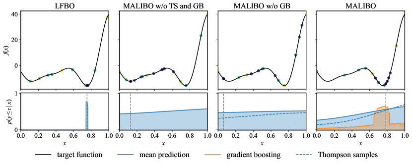
Figure 13: Task adaptation of different MALIBO variants on quadratic function after meta-learning. Each method optimize for $16$ iterations

Comparison on benchmark results

We compare the performance of MALIBO variants with different components on the NASBench201 as a representative example. As we can see in Figure 14, across all benchmarks on NASBench201, MALIBO (probit) converges quickly but fail to provide further improvement due to over-exploitation while MALIBO (TS) and MALIBO explore more and yield lower immediate regrets. However, the gradient boosting help MALIBO to converge faster than MALIBO (TS) after early exploration and therefore resulting in best final performance among the three.

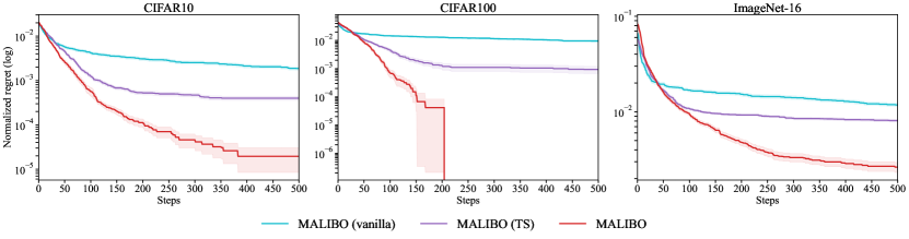
Figure 14: Results of MALIBO and its variants for the NASBench201 benchmarks.

E.3 Effects of different inference methods

In this section, we investigate the performance of different methods for approximating the posterior task embedding $p(\mathbf{z}\mid\mathcal{D}_{N})$. Specifically, we compare three different inference methods: Hamiltonian Monte Carlo (HMC), stochastic variational inference (SVI) and the Laplace approximation. We construct two variants of MALIBO, which are MALIBO (SVI) and MALIBO (HMC) by replacing the Laplace approximation with the corresponding inference method.

Compared to the Laplace approximation, SVI and HMC normally take longer time for the approximation, especially for HMC, since it needs multiple samples to estimate the expectation. To show their speed and scalability, we compare their runtime on NASBench201 in Figure 15 and show that the MALIBO with Laplace approximation takes around $0.1$ second for every iteration, while MALIBO (SVI) takes around $10$ seconds and MALIBO (HMC) $100$ seconds. Although the SVI and HMC variants take longer time for inference, we show that the performance among these methods are close in Figure 16. Similar behaviors are also observed in other benchmarks, including the HPOBench and MLBench. Due to the fast inference time and competitive performance, we use Laplace approximation as our proposed inference method for MALIBO.

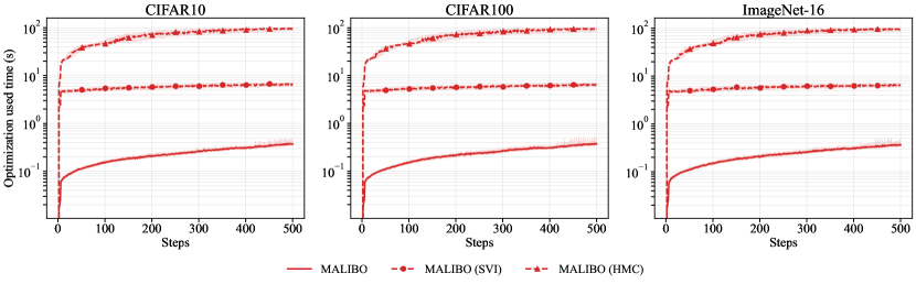
Figure 15: Runtime of different MALIBO variants over optimization steps on NASBench201. We show the typical results for CIFAR-10 benchmark and plot the medial inter-quantiles to remove outliers

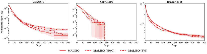
Figure 16: Normalized regrets of different MALIBO variants on the NASBench201 neural network architecture search problem. Each algorithm runs for 200 iterations and we show the corresponding estimated wall-clock time on the $x$ axis in log scale.

Appendix F Step-through visualization

For illustration purposes, we provide step-through visualizations on a Forrester function. For details of the synthetic functions, we refer to Appendix I. We use the same meta-trained model for the visualizations as the one used in Section E.1 for the corresponding problem.

Sequential BO

For the step-through visualization, the initial design is provided by the highest utility value of the mean predictions. After the first proposed query, we collect our the observations for the following 4 iterations using only the Thompson samples of the acquisition function. This is because we need to provide enough data to train and apply early stopping for our gradient boosting classifier. We provide the step-through visualization in Figure 17.

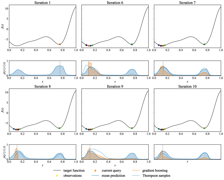
Figure 17: MALIBO optimizing a Forrester function. We show the mean prediction, the Thompson samples of the acquisition function and the gradient boosting prediction in the lower part of each sub-figure. At the first iteration, MALIBO picks the point with highest mean prediction of the acquisition function, which is often already close to the global optimum. Thereafter, we collect 4 more observations via the maximum prediction of a Thompson sample, in order to have sufficient data to train and apply early stopping for the gradient boosting model. Observations picked by Thompson samples show that MALIBO explores another location of interest on the left-hand side and also area close to the true optimum. With gradient boosting, the model is still able to explore the function and the predictions on non promising area are suppressed in later iterations.

Parallel BO with Thompson sampling

After showing the step-through visualization for MALIBO, we try to showcase a preliminary experiments about extending MALIBO to parallel BO. We show a toy examples of synchronous parallel BO [32] using MALIBO (TS) on the same function. To be specific, we use three Thompson samples as acquisition functions in each iteration, and evaluates the three proposed points for the next optimization step. We demonstrate that, MALIBO can be easily extended to parallel BO with the help of Thompson sampling.

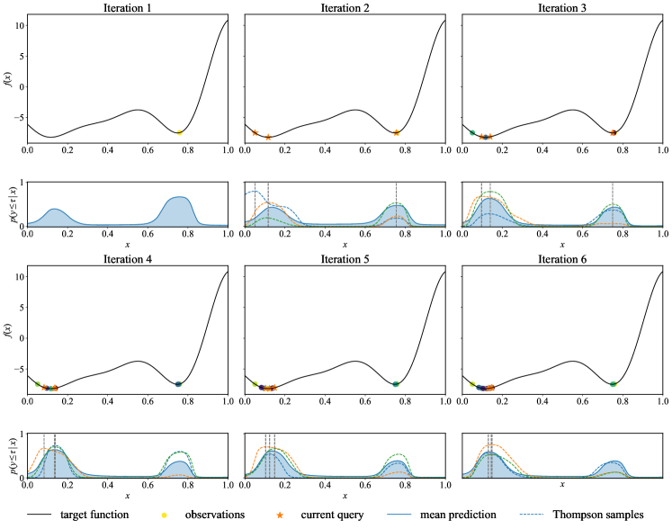
Figure 18: Synchronous parallel Thompson sampling using MALIBO (TS) to optimize a Forrester function. At every iteration, three samples are drawn as acquisition functions and utilized to the determine the next query points. In the first iteration, MALIBO (TS) already acquires three observations which cover both likely positions for the optimum. Subsequently, MALIBO (TS) exploits more often around the area where the true optimum is located. At the last iteration, all of the three Thompson samples have already been skew toward the left-hand side, which shows MALIBO (TS) converges to the correct region.

Appendix G Additional results

In this section we show the full results for the benchmarks in Section 5. With the settings remaining the same, we show the results on all HPOBench benchmarks in Figure 19, NASBench201 in Figure 20 and MLBench in Figure 21. For the noise robustness experiment with heteroscedastic noise, we include more experiments on Forrester [55] and Branin [11] function ensembles. We refer to Appendices I and I respectively for more details about the synthetic function benchmarks.

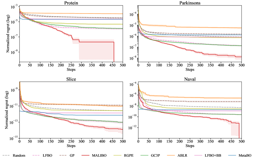
Figure 19: Normalized regret for different BO algorithms on the HPOBench neural network tuning problems ($D=9$) for $4$ datasets. The optimization objective in this benchmark is the validation loss.

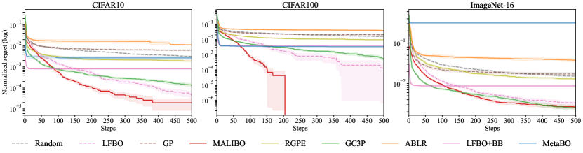
Figure 20: Normalized regret for different BO algorithms on the NASBench201 neural archtecture search problems ($D=6$) for $3$ datasets. The optimization objective in this benchmark is the validation accuracy.

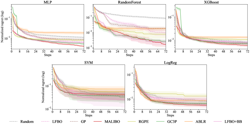
Figure 21: Normalized regret for different BO algorithms on hyperparameter tuning problems for $5$ different machine learning algorithms. The optimization objective in this benchmark is the validation accuracy.

Forrester function ensemble

For meta-training in Forester ensemble experiment, we randomly sampled noisy $32$ observations in $64$ related-tasks. The results is shown in Figure 22. MALIBO keep showing strong warm-starting performance and stay robust to noise compared to other methods. However, all the likelihood-free BO methods, namely LFBO, LFBO+BB and MALIBO, seem to stuck in local minimum in some runs, resulting in almost no improvement over the optimization process. The performance of MALIBO is on-par with GC3P in all cases. Although most of the GP-based methods, namely GP, RGPE and ABLR, all outperform the other likelihood-free based methods, however after increasing the noise level, their performances degrade significantly.

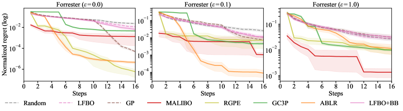
Figure 22: Normalized regret for different BO algorithms on Forrester function ensembles ($D=1$) with different levels of multiplicative noise.

Branin function ensemble

We randomly sampled noisy $128$ observations in $256$ related-tasks in the Branin ensemble experiment. The results is shown in Figure 23. MALIBO shows the strongest meta-learning performance in all settings and more robust than most of the regression-based methods. RGPE remains robust to the noise changes and consistently show the best final performance due to its rank-weighted algorithm. The other GP-based methods and ABLR, although they have strong performance in the noise-free case, but they degrade significantly after the noise level increased.

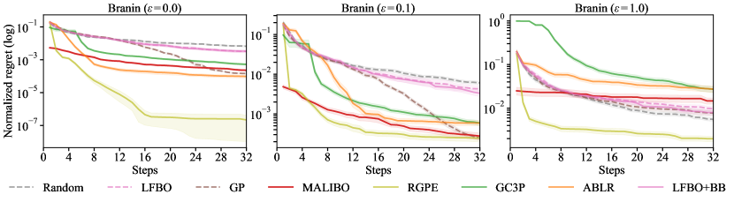
Figure 23: Normalized regret for different BO algorithms on Branin function ensembles ($D=2$) with different levels of multiplicative noise.

Appendix H Experimental details

In this section, we explain the setups for all baselines we used in the experiments. We ran all baselines on 4 CPUs (Intel(R) Xeon(R) Gold 6150 CPU @ 2.70GHz) except for MetaBO, which requires more computation and we explain the details down below.

GP-UCB

We use the SingleTaskGP implementation from BoTorch with Matérn $5/2$ kernel and UCB [58] as acquisition function. We set the hyperparameter $\beta=9.0$ in UCB, which controls the upper bound of the posterior standard deviation.

LFBO

Our implementation of LFBO is based on the official repository from Song et al. [56] and we use gradient boosting from scikit-learn [45] as the classifier with the following settings: $\text{n\_estimator}=100$, $\text{learning rate}=0.1$, $\text{min\_samples\_split}=2$, $\text{min\_samples\_leaf}=1$. For each problem, LFBO first randomly samples $1$0 observations to gather information and thereafter perform optimization using the classifier. For the threshold $\gamma$, which trade-off the exploration and exploitation, we set $\gamma=1/3$ following Song et al. [56] for all experiments. To maximize the resulting acquisition function, we use random search with $5,120$ samples following Tiao et al. [61], where they show that, the acquisition function is usually non-smooth and discontinuous for decision trees based method and using random search is on par and even outperforms the more expensive alternative evolutionary algorithm.

LFBO+BB

We extend LFBO to a meta-learning method with bounding box search space pruning [47], which reduces the search space based on the promising configurations in the related tasks. Our implementation of the search space pruning technique is based on the open-source implementation in Syne Tune. To construct the bounding box, we select the top-$1$ performing configurations from each related task, and truncate the search space according to the these configurations. We then apply LFBO to optimize the target task in the pruned search space.

RGPE

BO optimizer that uses a ranking-weighted GP ensemble (RGPE) as surrogate model and our implementation is based on Feurer et al. [17]. The key idea behind the algorithm is, that for optimization, the important information predicted by the surrogate model is not so much the function value $f(\mathbf{x})$ at a given input $\mathbf{x}$, but rather if the value $f(\mathbf{x})$ is larger or smaller relative to the function evaluated at other inputs. In other words, whether $f(\mathbf{x})>f(\mathbf{x}^{\prime})$ or vice versa.

ABLR

BO with multi-task adaptive Bayesian linear regression. Our implementation of ABLR is equivalent to a GP with 0 mean and a dot-product kernel with learned basis functions. We use a neural net (NN) with 2 (50, 50) hidden layers and tanh activation as the basis functions. We then train ABLR by optimizing the negative log likelihood (NLL) over NN weights and covariance matrix that define the dot-product kernel.

GC3P

We use the open-source implementation for GC3P from Salinas et al. [50]. For each target function, GC3P first samples five candidates from a meta-learned NN model before building a task-specific Copula process.

MetaBO

The training and evaluation of MetaBO was done based on the official implementation of Volpp et al. [65]. We followed the recommended hyperparameters and model architecture from the implementation with the following changes:

1. We extended the training horizon to 60 steps, which is longer than the ones used by Volpp et al. [65]. We chose the longer episode length to adapt to the higher dimensional space and the evaluation horizon we chose for the benchmarks. The value 60 was chosen as a compromise between the full evaluation length of 500 iterations and the resulting increase in training time due to the scaling of the GP used in the method.

2. We did not include the current time-step and total budget as features to the neural network policy due to poor performance on our benchmarks when including them.

3. Due to the small number of data sets, we estimated the GP hyperparameters with independent sub-samples of the meta-data sets, but otherwise following the procedure of Volpp et al. [65]. This effectively gives MetaBO access to more meta-data, but is consistent with the evaluation scheme described below.

Besides these changes to the method, we also employed a different evaluation scheme for MetaBO due to its high training cost. In contrast to the other meta-learning models that train in minutes on the meta-data using a single CPU, MetaBO required almost 2 hours, using one NVIDIA Titan X GPU and 10 Intel(R) Xeon(R) CPU E5-2697 v3CPUs. This made the independent meta-training across the individual runs infeasible. To still include MetaBO into some of our benchmarks, we decided to train MetaBO once and reuse this model throughout the individual runs during the evaluation.

During the meta-training, MetaBO received the same number of samples per meta-task as the other methods, but the subsample was resampled for each training episode. While this gave MetaBO access to more meta-data compared to the other methods, we eliminated the risk of evaluating the method on a bad subsample of the data by chance.

The advantage of effectively seeing more points of each meta-tasks should be considered when evaluating the early performance of MetaBO compared to the other methods. The evidently weak adaptation of MetaBO to new tasks dissimilar to the meta-data.

Based on the high meta-training cost of MetaBO and the relatively poor performance on NASBench201 and the HPOBench benchmarks, we decided to not include the method for the other evaluations, as scheme of leave-one-task-out validation would be too expensive and any other comparison would either benefit MetaBO or put it at a disadvantage rendering the results difficult to interpret.

MALIBO

We use a Residual Feed Forward Network (ResFFN) [26] to learn the latent feature representation, with $4$ hidden layers, each with $64$ units. For the mean prediction layer $m(\cdot)$ and task-specific layer, we use a fully connected layer with $50$ units for each. The resulting meta-leaning model has $22,359$ learnable parameters. We use ELU [10] as the activation function in the network following Tiao et al. [61]. Similar to LFBO, we set the threshold $\gamma=1/3$ and maximize the acquisition function using random search with $5,120$ samples..

During meta-training, we optimize the parameters in the network with the ADAM optimizer [34], with learning rate $\text{lr}=10^{-3}$ and batch size of $B=256$. In addition, we apply exponential decay to the learning rate in each epoch with factor of $0.999$. The model is trained for $2,048$ epochs with early stopping. For the regularization loss, we set the regularization factor $\lambda=0.1$ in Equation 3 and follow the approach in Appendix C to estimate the coefficients $\lambda_{\text{KS}}$ and $\lambda_{\text{Cov}}$. The resulting meta-training is fast and efficient and we show the training time as well as the amount of meta-data for each benchmark in Table 1.

In task adaptation, we optimize the task embedding for the target task using L-BFGS [8]. After obtaining the model adapted on target task, we combine it with a gradient boosting classifier, which serves as a residual prediction model. We use the same setting for the gradient boosting as in LFBO, except that we use the meta-learned MALIBO classifier as the initial estimator. However, the gradient boosting classifier is trained only on the observations generated by the optimization process, which might lead to overfitting on limited amount of data during early iterations. Therefore, we apply early stopping to avoid such behavior. Specifically, we first estimate the number of trees that we need for training without overfitting. This is done by fitting a gradient boosting classifier with randomly chosen training data and validation data, which account for $70\%$ and $30\%$ of the whole data respectively. The resulting classifier estimates the number of trees that are needed to fit the partially observed data while offering good generalization ability. We then use it as our hyperparameter for the gradient boosting and train it on all observations.

Table 1: Meta-data and training time

Benchmark	Number of meta-data	Training time
HPOBench	$1,536$	around 15 seconds
NASBench201	$1,024$	around 15 seconds
MLBench	$2,432$	around 30 seconds
Branin	$32,768$	around 480 seconds
Hartmann3	$131,072$	around 1,800 seconds

Appendix I Details of benchmarks

HPOBench

The hyperparameters for HPOBench and their ranges are demonstrated in Table 2. All hyperparameters are discrete and there are in total $66208$ possible combinations. More details can be found in Klein and Hutter [35].

Table 2: Configuration spaces for HPOBench

Hyperparameter	Range
Initial LR	{ $5\times 10^{-4}$, $1\times 10^{-3}$, $5\times 10^{-3}$, $1\times 10^{-2}$, $5\times 10^{-2}$, $1\times 10^{-1}$ }
LR Schedule	{ cosine, fixed }
Batch size	{ $2^{3}$, $2^{4}$, $2^{5}$, $2^{6}$ }
Layer 1 Width	{ $2^{4}$, $2^{5}$, $2^{6}$, $2^{7}$, $2^{8}$, $2^{9}$ }
Activation	{ relu, tanh }
Dropout rate	{ $0.0$, $0.3$, $0.6$ }
Layer 2 Width	{ $2^{4}$, $2^{5}$, $2^{6}$, $2^{7}$, $2^{8}$, $2^{9}$ }
Activation	{ relu, tanh }
Dropout rate	{ $0.0$, $0.3$, $0.6$ }

ML algorithms in HPOBench

The hyperparameters for machine learning (ML) algorithms in HPOBench [14] and their ranges are summarized in Table 3. More details can be found in Eggensperger et al. [14].

Table 3: Configuration spaces for ML algorithms in HPOBench

Benchmark	Hyperparameter	type	Log	Range
SVM	C	float	✓	[ $2^{-10}$, $2^{10}$ ]
	gamma	float	✓	[ $2^{-10}$, $2^{10}$ ]
LogReg	alpha	float	✓	[ $1e^{-5}$, $1.0$ ]
	eta0	float	✓	[ $1e^{-5}$, $1.0$ ]
XGBoost	colsample_bytree	float	✗	[ $0.1$, $1.0$ ]
	eta	float	✓	[ $2^{-10}$, $1.0$ ]
	max_depth	int	✓	[ $1$, $50$ ]
	reg_lambda	float	✓	[ $2^{-10}$, $2^{-10}$ ]
RandomForest	max_depth	int	✓	[ $1$, $50$ ]
	max_features	float	✗	[ $0.0$, $1.0$ ]
	min_samples_leaf	int	✗	[ $1$, $2$ ]
	min_samples_split	int	✓	[ $2$, $128$ ]
MLP	alpha	float	✓	[ $1.0e^{-8}$, $1.0$ ]
	batch_size	int	✓	[ $4$, $256$ ]
	depth	int	✗	[ $1$, $3$ ]
	learning_rate_init	float	✓	[ $1.0e^{-5}$, $1.0$ ]
	width	int	✓	[ $16$, $1024$ ]

NASBench201

The hyperparameters for NASBench201 and their ranges are summarized in Table 4. All hyperparameters are discrete and there are in total $15625$ possible combinations. More details can be found in Dong and Yang [12].

Table 4: Configuration spaces for NASBench201

Hyperparameter	Range
ARC 0	{ none, skip-connect, conv-$1\times 1$, conv-$3\times 3$, avg-pool-$3\times 3$ }
ARC 1	{ none, skip-connect, conv-$1\times 1$, conv-$3\times 3$, avg-pool-$3\times 3$ }
ARC 2	{ none, skip-connect, conv-$1\times 1$, conv-$3\times 3$, avg-pool-$3\times 3$ }
ARC 3	{ none, skip-connect, conv-$1\times 1$, conv-$3\times 3$, avg-pool-$3\times 3$ }
ARC 4	{ none, skip-connect, conv-$1\times 1$, conv-$3\times 3$, avg-pool-$3\times 3$ }
ARC 5	{ none, skip-connect, conv-$1\times 1$, conv-$3\times 3$, avg-pool-$3\times 3$ }

The Quadratic Ensemble

The function for the quadratic ensemble is defined as:

$$f(x,a,b,c)=(a\cdot(x-b))^{2}-c\qquad x\in[0,1]$$ (30)

To form the ensemble, we choose the distribution for the parameters as:

$$a\sim\mathcal{U}(0.5,1.5)\quad b\sim\mathcal{U}(-0.9,0.9)\quad c\sim\mathcal{U}(-1,1)$$ (31)

This distribution of parameters ensures that the search space contains the minimum of the quadratic function at $x^{*}=b$ with $f(x^{*})=c$. The location of the optimum has a broad distribution over the function space, which is intended to highlight algorithms that learn the global structure of the ensemble rather than restricting on some small regions of interest.

The Forrester Ensemble

The original Forrester function [55] is defined following:

$$f(x,a,b,c)=a\cdot(6x-2)^{2}\dot{\sin}(12x-4)+b(x-0.5)-c\qquad x\in[0,1]$$ (32)

The function has one local and one global minimum, and a zero-gradient inflection point in the domain $x\in[0,1]$. To form the ensemble, we choose the distribution for the parameters as:

$$a\sim\mathcal{U}(0.2,3)\quad b\sim\mathcal{U}(-5,15)\quad c\sim\mathcal{U}(-5,5)$$ (33)

Let $\tau=\{a,b,c\}$ and $p(\tau)$ is a three dimensional uniform distribution. The ranges are chosen around the usually used fixed values for the parameters, namely $a=0.5$, $b=10$, $c=-5$.

The Branin Ensemble

The function for the Branin ensemble is the following:

$$f(x,a,b,c)=a(x_{2}-bx_{1}^{2}+cx_{1}-r)+s(1-t)\cos(x_{1})+s\qquad x_{1}\in[-5,10],x_{2}\in[0,15]$$ (34)

The distribution for the parameters are chosen as:

$$\begin{split}&a\sim\mathcal{U}(0.5,1.5)\quad b\sim\mathcal{U}(0.1,0.15)\quad c\sim\mathcal{U}(1.0,2.0)\\ &r\sim\mathcal{U}(5.0,7,0)\quad s\sim\mathcal{U}(8.0,12.0)\quad t\sim\mathcal{U}(0.03,0.05)\end{split}$$ (35)

Let $\tau=\{a,b,c,r,s,t\}$ and $p(\tau)$ is a six dimensional uniform distribution. The ranges are chosen around the usually used fixed values for the parameters, namely $a=1$, $b=5.1/(4\pi^{2})$, $c=5/\pi$, $r=6$, $s=10$ and $t=1/(8\pi)$.

The Hartmann3 Ensemble

The function for Hartmann3 [11] ensemble reads:

$$\begin{split}&f(x,\alpha_{1},\alpha_{2},\alpha_{3},\alpha_{4})=-\sum^{4}_{i=1}\alpha_{i}\exp\left(-\sum^{3}_{j=1}A_{i,j}(x_{j}-P_{i,j})^{2}\right)\qquad x\in[0,1]\\ &\bm{A}=\begin{bmatrix}3.0&10&30\\ 0.1&10&35\\ 3.0&10&30\\ 0.1&10&35\end{bmatrix}\qquad\bm{P}=10^{-4}\cdot\begin{bmatrix}3689&1170&2673\\ 4699&4387&7470\\ 1091&8732&5547\\ 381&5743&8828\end{bmatrix}\end{split}$$ (36)

To form the ensemble, we choose the distribution for the parameters as:

$$\alpha_{1}\sim\mathcal{U}(0.0,2.0)\quad\alpha_{2}\sim\mathcal{U}(0.0,2.0)\quad\alpha_{3}\sim\mathcal{U}(2.0,4.0)\quad\alpha_{4}\sim\mathcal{U}(2.0,4.0)$$ (37)

Let $\tau=\{\alpha_{1},\alpha_{2},\alpha_{3},\alpha_{4}\}$ and $p(\tau)$ is a four dimensional uniform distribution.

References

- Andrychowicz et al. [2016] Marcin Andrychowicz, Misha Denil, Sergio Gómez Colmenarejo, Matthew W. Hoffman, David Pfau, Tom Schaul, Brendan Shillingford, and Nando de Freitas. Learning to learn by gradient descent by gradient descent. In Proceedings of the 30th International Conference on Neural Information Processing Systems, NIPS’16, page 3988–3996. Curran Associates Inc., 2016.
- Bardenet et al. [2013] Rémi Bardenet, Mátyás Brendel, Balázs Kégl, and Michèle Sebag. Collaborative hyperparameter tuning. In Proceedings of the 30th International Conference on International Conference on Machine Learning - Volume 28, ICML’13, page II–199–II–207. JMLR.org, 2013.
- Bergstra and Bengio [2012] James Bergstra and Yoshua Bengio. Random search for hyper-parameter optimization. J. Mach. Learn. Res., 13(null):281–305, 2012.
- Bergstra et al. [2011] James Bergstra, Rémi Bardenet, Yoshua Bengio, and Balázs Kégl. Algorithms for hyper-parameter optimization. In Advances in Neural Information Processing Systems, volume 24. Curran Associates, Inc., 2011.
- Berkenkamp et al. [2021] Felix Berkenkamp, Anna Eivazi, Lukas Grossberger, Kathrin Skubch, Jonathan Spitz, Christian Daniel, and Stefan Falkner. Probabilistic meta-learning for bayesian optimization, 2021. URL https://openreview.net/forum?id=fdZvTFn8Yq.
- Bishop and Nasrabadi [2006] Christopher M Bishop and Nasser M Nasrabadi. Pattern recognition and machine learning. Springer, 2006.
- Blundell et al. [2015] Charles Blundell, Julien Cornebise, Koray Kavukcuoglu, and Daan Wierstra. Weight uncertainty in neural networks. In Proceedings of the 32nd International Conference on International Conference on Machine Learning - Volume 37, ICML’15, page 1613–1622, 2015.
- Byrd et al. [1995] Richard H. Byrd, Peihuang Lu, Jorge Nocedal, and Ciyou Zhu. A limited memory algorithm for bound constrained optimization. SIAM Journal on Scientific Computing, 16(5):1190–1208, 1995.
- Chrabaszcz et al. [2017] Patryk Chrabaszcz, Ilya Loshchilov, and Frank Hutter. A downsampled variant of imagenet as an alternative to the cifar datasets. arXiv preprint arXiv:1707.08819, 2017.
- Clevert et al. [2016] Djork-Arné Clevert, Thomas Unterthiner, and Sepp Hochreiter. Fast and accurate deep network learning by exponential linear units (elus). In 4th International Conference on Learning Representations, ICLR 2016, San Juan, Puerto Rico, May 2-4, 2016, 2016.
- Dixon [1978] Laurence Charles Ward Dixon. The global optimization problem. an introduction. Toward global optimization, 2:1–15, 1978.
- Dong and Yang [2020] Xuanyi Dong and Yi Yang. Nas-bench-201: Extending the scope of reproducible neural architecture search. In International Conference on Learning Representations, 2020.
- Dua and Graff [2017] Dheeru Dua and Casey Graff. UCI machine learning repository, 2017. URL http://archive.ics.uci.edu/ml.
- Eggensperger et al. [2021] Katharina Eggensperger, Philipp Müller, Neeratyoy Mallik, Matthias Feurer, Rene Sass, Aaron Klein, Noor Awad, Marius Lindauer, and Frank Hutter. HPOBench: A collection of reproducible multi-fidelity benchmark problems for HPO. In Thirty-fifth Conference on Neural Information Processing Systems Datasets and Benchmarks Track (Round 2), 2021.
- Feurer et al. [2014] Matthias Feurer, Jost Tobias Springenberg, and Frank Hutter. Using meta-learning to initialize bayesian optimization of hyperparameters. In Proceedings of the 2014 International Conference on Meta-Learning and Algorithm Selection - Volume 1201, MLAS’14, page 3–10, Aachen, DEU, 2014. CEUR-WS.org.
- Feurer et al. [2018a] Matthias Feurer, Benjamin Letham, and Eytan Bakshy. Scalable meta-learning for bayesian optimization using ranking-weighted gaussian process ensembles. In ICML 2018 AutoML Workshop, 2018a.
- Feurer et al. [2018b] Matthias Feurer, Benjamin Letham, Frank Hutter, and Eytan Bakshy. Practical transfer learning for bayesian optimization. arXiv preprint arXiv:1802.02219, 2018b.
- Finn et al. [2017] Chelsea Finn, Pieter Abbeel, and Sergey Levine. Model-agnostic meta-learning for fast adaptation of deep networks. In Proceedings of the 34th International Conference on Machine Learning, volume 70 of Proceedings of Machine Learning Research, pages 1126–1135. PMLR, 06–11 Aug 2017.
- Finn et al. [2018] Chelsea Finn, Kelvin Xu, and Sergey Levine. Probabilistic model-agnostic meta-learning. In Advances in Neural Information Processing Systems, volume 31. Curran Associates, Inc., 2018.
- Frazier et al. [2009] Peter Frazier, Warren Powell, and Savas Dayanik. The knowledge-gradient policy for correlated normal beliefs. INFORMS journal on Computing, 21(4):599–613, 2009.
- Frazier and Wang [2015] Peter I Frazier and Jialei Wang. Bayesian optimization for materials design. In Information science for materials discovery and design, pages 45–75. Springer, 2015.
- Friedman [2001] Jerome H. Friedman. Greedy function approximation: A gradient boosting machine. The Annals of Statistics, 29(5):1189 – 1232, 2001.
- Garnett [2022] Roman Garnett. Bayesian Optimization. Cambridge University Press, 2022.
- Golovin et al. [2017] Daniel Golovin, Benjamin Solnik, Subhodeep Moitra, Greg Kochanski, John Karro, and D. Sculley. Google vizier: A service for black-box optimization. In Proceedings of the 23rd ACM SIGKDD International Conference on Knowledge Discovery and Data Mining, KDD ’17, page 1487–1495. Association for Computing Machinery, 2017.
- Graves [2011] Alex Graves. Practical variational inference for neural networks. In Advances in Neural Information Processing Systems, volume 24, 2011.
- He et al. [2016] Kaiming He, Xiangyu Zhang, Shaoqing Ren, and Jian Sun. Deep residual learning for image recognition. In 2016 IEEE Conference on Computer Vision and Pattern Recognition (CVPR), pages 770–778, 2016.
- Hennig and Schuler [2012] Philipp Hennig and Christian J Schuler. Entropy search for information-efficient global optimization. Journal of Machine Learning Research, 13(6), 2012.
- Hernández-Lobato et al. [2014] José Miguel Hernández-Lobato, Matthew W Hoffman, and Zoubin Ghahramani. Predictive entropy search for efficient global optimization of black-box functions. Advances in neural information processing systems, 27, 2014.
- Homan and Gelman [2014] Matthew D. Homan and Andrew Gelman. The no-u-turn sampler: Adaptively setting path lengths in hamiltonian monte carlo. J. Mach. Learn. Res., 15(1):1593–1623, 2014.
- Huang et al. [2020] Kaixuan Huang, Yuqing Wang, Molei Tao, and Tuo Zhao. Why do deep residual networks generalize better than deep feedforward networks? — a neural tangent kernel perspective. In Advances in Neural Information Processing Systems, volume 33, pages 2698–2709, 2020.
- Hutter et al. [2019] Frank Hutter, Lars Kotthoff, and Joaquin Vanschoren. Automated Machine Learning: Methods, Systems, Challenges. Springer Publishing Company, Incorporated, 2019.
- Kandasamy et al. [2018] Kirthevasan Kandasamy, Akshay Krishnamurthy, Jeff Schneider, and Barnabas Poczos. Parallelised bayesian optimisation via thompson sampling. In Amos Storkey and Fernando Perez-Cruz, editors, Proceedings of the Twenty-First International Conference on Artificial Intelligence and Statistics, volume 84 of Proceedings of Machine Learning Research, pages 133–142. PMLR, 2018.
- Kim et al. [2017] Jungtaek Kim, Saehoon Kim, and Seungjin Choi. Learning to warm-start bayesian hyperparameter optimization. arXiv preprint arXiv:1710.06219, 2017.
- Kingma and Ba [2015] Diederik P. Kingma and Jimmy Ba. Adam: A method for stochastic optimization. In 3rd International Conference on Learning Representations, ICLR 2015, San Diego, CA, USA, May 7-9, 2015, Conference Track Proceedings, 2015.
- Klein and Hutter [2019] Aaron Klein and Frank Hutter. Tabular benchmarks for joint architecture and hyperparameter optimization. arXiv preprint arXiv:1905.04970, 2019.
- Krizhevsky et al. [2009] Alex Krizhevsky, Geoffrey Hinton, et al. Learning multiple layers of features from tiny images. online, 2009.
- Kushner [1964] H. J. Kushner. A New Method of Locating the Maximum Point of an Arbitrary Multipeak Curve in the Presence of Noise. Journal of Basic Engineering, 86(1):97–106, 03 1964.
- Li et al. [2022] Yang Li, Yu Shen, Huaijun Jiang, Tianyi Bai, Wentao Zhang, Ce Zhang, and Bin Cui. Transfer learning based search space design for hyperparameter tuning. In Proceedings of the 28th ACM SIGKDD Conference on Knowledge Discovery and Data Mining, KDD ’22, page 967–977, 2022.
- Marco et al. [2017] Alonso Marco, Felix Berkenkamp, Philipp Hennig, Angela P. Schoellig, Andreas Krause, Stefan Schaal, and Sebastian Trimpe. Virtual vs. real: Trading off simulations and physical experiments in reinforcement learning with bayesian optimization. In 2017 IEEE International Conference on Robotics and Automation (ICRA), page 1557–1563. IEEE Press, 2017.
- Močkus [1975] J. Močkus. On bayesian methods for seeking the extremum. In Optimization Techniques IFIP Technical Conference Novosibirsk, July 1–7, 1974, pages 400–404. Springer Berlin Heidelberg, 1975.
- Murphy [2012] Kevin P. Murphy. Machine Learning: A Probabilistic Perspective. The MIT Press, 2012.
- Neal [1996] Radford M. Neal. Bayesian Learning for Neural Networks. Springer-Verlag, 1996.
- Nguyen et al. [2010] XuanLong Nguyen, Martin J. Wainwright, and Michael I. Jordan. Estimating divergence functionals and the likelihood ratio by convex risk minimization. IEEE Transactions on Information Theory, 56(11):5847–5861, nov 2010.
- Oliveira et al. [2022] Rafael Oliveira, Louis C. Tiao, and Fabio Ramos. Batch bayesian optimisation via density-ratio estimation with guarantees. In Advances in Neural Information Processing Systems, 2022.
- Pedregosa et al. [2011] F. Pedregosa, G. Varoquaux, A. Gramfort, V. Michel, B. Thirion, O. Grisel, M. Blondel, P. Prettenhofer, R. Weiss, V. Dubourg, J. Vanderplas, A. Passos, D. Cournapeau, M. Brucher, M. Perrot, and E. Duchesnay. Scikit-learn: Machine learning in Python. Journal of Machine Learning Research, 12:2825–2830, 2011.
- Perrone et al. [2018] Valerio Perrone, Rodolphe Jenatton, Matthias W Seeger, and Cedric Archambeau. Scalable hyperparameter transfer learning. In Advances in Neural Information Processing Systems, volume 31. Curran Associates, Inc., 2018.
- Perrone et al. [2019] Valerio Perrone, Huibin Shen, Matthias Seeger, Cédric Archambeau, and Rodolphe Jenatton. Learning search spaces for bayesian optimization: Another view of hyperparameter transfer learning. In Proceedings of the 33rd International Conference on Neural Information Processing Systems. Curran Associates Inc., 2019.
- Qin [1998] Jing Qin. Inferences for case-control and semiparametric two-sample density ratio models. Biometrika, 85(3):619–630, 1998.
- Rasmussen [2004] Carl Edward Rasmussen. Gaussian Processes in Machine Learning. Springer Berlin Heidelberg, 2004.
- Salinas et al. [2020] David Salinas, Huibin Shen, and Valerio Perrone. A quantile-based approach for hyperparameter transfer learning. In Proceedings of the 37th International Conference on Machine Learning, volume 119 of Proceedings of Machine Learning Research, pages 8438–8448. PMLR, 2020.
- Salinas et al. [2023] David Salinas, Jacek Golebiowski, Aaron Klein, Matthias Seeger, and Cedric Archambeau. Optimizing hyperparameters with conformal quantile regression. arXiv preprint arXiv:2305.03623, 2023.
- Saseendran et al. [2021] Amrutha Saseendran, Kathrin Skubch, Stefan Falkner, and Margret Keuper. Shape your space: A gaussian mixture regularization approach to deterministic autoencoders. In Advances in Neural Information Processing Systems, volume 34, pages 7319–7332. Curran Associates, Inc., 2021.
- Schilling et al. [2016] Nicolas Schilling, Martin Wistuba, and Lars Schmidt-Thieme. Scalable hyperparameter optimization with products of gaussian process experts. In ECML/PKDD, 2016.
- Shahriari et al. [2016] Bobak Shahriari, Kevin Swersky, Ziyu Wang, Ryan P. Adams, and Nando de Freitas. Taking the human out of the loop: A review of bayesian optimization. Proceedings of the IEEE, 104(1):148–175, 2016.
- Sobester et al. [2008] András Sobester, Alexander Forrester, and Andy Keane. Engineering design via surrogate modelling: a practical guide. John Wiley & Sons, 2008.
- Song et al. [2022] Jiaming Song, Lantao Yu, Willie Neiswanger, and Stefano Ermon. A general recipe for likelihood-free Bayesian optimization. In Proceedings of the 39th International Conference on Machine Learning, volume 162, pages 20384–20404. PMLR, 2022.
- Springenberg et al. [2016] Jost Tobias Springenberg, Aaron Klein, Stefan Falkner, and Frank Hutter. Bayesian optimization with robust bayesian neural networks. In Advances in Neural Information Processing Systems, volume 29. Curran Associates, Inc., 2016.
- Srinivas et al. [2010] Niranjan Srinivas, Andreas Krause, Sham Kakade, and Matthias Seeger. Gaussian process optimization in the bandit setting: No regret and experimental design. In Proceedings of the 27th International Conference on International Conference on Machine Learning, ICML’10, page 1015–1022. Omnipress, 2010.
- Sugiyama et al. [2012] Masashi Sugiyama, Taiji Suzuki, and Takafumi Kanamori. Density Ratio Estimation in Machine Learning. Cambridge University Press, 2012.
- Swersky et al. [2013] Kevin Swersky, Jasper Snoek, and Ryan P Adams. Multi-task bayesian optimization. In C.J. Burges, L. Bottou, M. Welling, Z. Ghahramani, and K.Q. Weinberger, editors, Advances in Neural Information Processing Systems, volume 26. Curran Associates, Inc., 2013.
- Tiao et al. [2021] Louis C Tiao, Aaron Klein, Matthias W Seeger, Edwin V. Bonilla, Cedric Archambeau, and Fabio Ramos. Bore: Bayesian optimization by density-ratio estimation. In Proceedings of the 38th International Conference on Machine Learning, volume 139, pages 10289–10300. PMLR, 2021.
- Tighineanu et al. [2022] Petru Tighineanu, Kathrin Skubch, Paul Baireuther, Attila Reiss, Felix Berkenkamp, and Julia Vinogradska. Transfer learning with gaussian processes for bayesian optimization. In Proceedings of The 25th International Conference on Artificial Intelligence and Statistics, volume 151 of Proceedings of Machine Learning Research, pages 6152–6181, 2022.
- Vanschoren [2018] Joaquin Vanschoren. Meta-learning: A survey. arXiv preprint arXiv:1810.03548, 2018.
- Vanschoren et al. [2014] Joaquin Vanschoren, Jan N. van Rijn, Bernd Bischl, and Luis Torgo. Openml: Networked science in machine learning. SIGKDD Explor. Newsl., 15(2):49–60, jun 2014.
- Volpp et al. [2020] Michael Volpp, Lukas P. Fröhlich, Kirsten Fischer, Andreas Doerr, Stefan Falkner, Frank Hutter, and Christian Daniel. Meta-learning acquisition functions for transfer learning in bayesian optimization. In International Conference on Learning Representations, 2020.
- Wang and Jegelka [2017] Zi Wang and Stefanie Jegelka. Max-value entropy search for efficient bayesian optimization. In International Conference on Machine Learning, pages 3627–3635. PMLR, 2017.
- Wang et al. [2022] Zi Wang, George E. Dahl, Kevin Swersky, Chansoo Lee, Zelda Mariet, Zachary Nado, Justin Gilmer, Jasper Snoek, and Zoubin Ghahramani. Pre-training helps bayesian optimization too. arXiv preprint arXiv:2207.03084, 2022.
- Weiss et al. [2016] Karl R. Weiss, Taghi M. Khoshgoftaar, and Dingding Wang. A survey of transfer learning. J. Big Data, 3:9, 2016.
- Wilson et al. [2018] James T. Wilson, Frank Hutter, and Marc Peter Deisenroth. Maximizing acquisition functions for bayesian optimization. In Proceedings of the 32nd International Conference on Neural Information Processing Systems, NIPS’18, page 9906–9917. Curran Associates Inc., 2018.
- Wistuba and Grabocka [2021] Martin Wistuba and Josif Grabocka. Few-shot bayesian optimization with deep kernel surrogates. In International Conference on Learning Representations, 2021.
- Wistuba et al. [2015] Martin Wistuba, Nicolas Schilling, and Lars Schmidt-Thieme. Learning hyperparameter optimization initializations. In 2015 IEEE International Conference on Data Science and Advanced Analytics (DSAA), pages 1–10, 2015.
- Wistuba et al. [2018] Martin Wistuba, Nicolas Schilling, and Lars Schmidt-Thieme. Scalable gaussian process-based transfer surrogates for hyperparameter optimization. Mach. Learn., 107(1):43–78, 2018.
- Yogatama and Mann [2014] Dani Yogatama and Gideon Mann. Efficient Transfer Learning Method for Automatic Hyperparameter Tuning. In Proceedings of the Seventeenth International Conference on Artificial Intelligence and Statistics, volume 33 of Proceedings of Machine Learning Research, pages 1077–1085. PMLR, 2014.