Physics-Constrained Hardware-Efficient Ansatz on Quantum Computers that is Universal, Systematically Improvable, and Size-consistent

Abstract

Variational wavefunction ansätze are at the heart of solving quantum many-body problems in physics and chemistry. Previous designs of hardware-efficient ansatz (HEA) on quantum computers are largely based on heuristics and lack rigorous theoretical foundations. In this work, we introduce a physics-constrained approach for designing HEA with rigorous theoretical guarantees by imposing a few fundamental constraints. Specifically, we require that the target HEA to be universal, systematically improvable, and size-consistent, which is an important concept in quantum many-body theories for scalability, but has been overlooked in previous designs of HEA. We extend the notion of size-consistency to HEA, and present a concrete realization of HEA that satisfies all these fundamental constraints while only requiring linear qubit connectivity. The developed physics-constrained HEA is superior to other heuristically designed HEA in terms of both accuracy and scalability, as demonstrated numerically for the Heisenberg model and some typical molecules. In particular, we find that restoring size-consistency can significantly reduce the number of layers needed to reach certain accuracy. In contrast, the failure of other HEA to satisfy these constraints severely limits their scalability to larger systems with more than ten qubits. Our work highlights the importance of incorporating physical constraints into the design of HEA for efficiently solving many-body problems on quantum computers.

University] Key Laboratory of Theoretical and Computational Photochemistry, Ministry of Education, College of Chemistry, Beijing Normal University, Beijing 100875, China

1 Introduction

Efficient simulation of quantum many-body problems is an enduring frontier in computational physics and chemistry¹. Among many different approaches, the variational method represents a powerful and versatile technique to tackle quantum many-body problems. A wealth of variational wavefunction ansätze on classical computers have been developed over the past decades. Prominent examples include Slater determinants, Gutzwiller wavefunction², Jastrow wavefunction³, tensor network states^{4, 5, 6, 7, 8, 9, 10}, and neural network states^{11, 12, 13, 14, 15, 16, 17}. Thanks to the rapid progress on quantum hardware^{18, 19}, the variational quantum eigensolver (VQE)^{20, 21}, which is a hybrid quantum-classical approach for solving quantum many-body problems²², has attracted much attention^{23, 24, 25, 26}. The central component of VQE is the preparation of a trial wavefunction on quantum computers, which ultimately determines the accuracy of the variational computation. Compared to the development of variational ansätze on classical computers, the exploration of wavefunction ansätze on quantum computers is still in its infancy.

Available variational ansätze on quantum computers developed so far can be broadly classified into two categories: physics/chemistry-inspired ansätze and hardware-efficient ansätze (HEA), each with its own advantages and disadvantages. The chemistry-inspired unitary coupled cluster (UCC) ansatz²⁷ is the first ansatz proposed for determining molecular ground states on quantum computers²⁰, which is motivated by the great success of the traditional coupled cluster theory on classical computers²⁸. However, it quickly becomes impractical for large molecules on the current noisy intermediate-scale quantum (NISQ) hardware²⁹, since the circuit depth scales as $O(N^{4})$ with respect to the number of qubits $N$^{30, 31, 32}. Many efforts have been devoted to reduce the complexity of UCC, resulting in several descendants of UCC such as the unitary paired CC ansatz³³, the unitary cluster Jastrow ansatz³⁴, and some adaptive variants^{35, 36, 37, 38}. Another type of physics-inspired ansatz is the Hamiltonian variational ansatz (HVA)^{39, 40}, which is problem specific and widely used for model systems⁴¹. When applied to general cases such as the molecular Hamiltonian in quantum chemistry, it suffers from the same problem as UCC.

Hardware efficient ansätze were originally proposed as a more practical alternative on near-term quantum devices⁴². It takes the following form

$$|\Psi\rangle=U_{L}(\vec{\theta}_{L})\cdots U_{1}(\vec{\theta}_{1})|\Phi_{0}\rangle\triangleq\prod_{l=1}^{L}U_{l}(\vec{\theta}_{l})|\Phi_{0}\rangle,$$ (1)

where $|\Phi_{0}\rangle$ is a reference state and the repeating unit $U_{l}(\vec{\theta}_{l})$ is a parameterized quantum circuit (PQC) composed of gates that are native on quantum hardware⁴², such as single-qubit rotation gates and two-qubit entangling gates (see Fig. 1a). Given the hardware constraints, there is still a great deal of freedom in choosing the layout of the circuit block $U_{l}(\vec{\theta}_{l})$. So far, the architectures of HEA have been designed mostly by heuristics, and there is no theoretical guarantee for their performance. Furthermore, the optimization of HEA is challenging⁴³ as the number of qubits $N$ and the number of layers $L$ increases, due to the proliferation of low-quality local minima⁴⁴ and the exponential vanishing of gradients, known as the ’barren plateau’ phenomenon⁴⁵. These problems severely limit the scalability of HEA beyond small systems. Therefore, it is highly desirable to design a variational ansatz with rigorous theoretical basis, while at the same time being hardware-efficient on near-term devices^{46, 47}.

In this work, we present a new way to design HEA with rigorous theoretical guarantees by imposing fundamental constraints. This is inspired by the remarkably successful way to design exchange-correlation (XC) functionals in density functional theories (DFT) by requiring the XC functionals to satisfy exact constraints⁴⁸, which has lead to reliable non-empirical XC functionals for a wide range of systems^{49, 50}. We expect that designing HEA in a similar way can lead to more systematic construction of variational ansätze on quantum computers. The remaining part of the paper is organized as follows: First, we introduce some fundamental constraints for HEA. Specifically, we require the ansatz to be universal, systematically improvable, and size-consistent (or multiplicatively separable), which is an important property for scalability in quantum many-body theory. Then, we present one concrete realization, which satisfies all these requirements while requiring only linear qubit connectivity with nearest neighbor interactions. Consequently, a layerwise optimization strategy is introduced to take full advantage of the systematic improvability of the proposed ansatz, which is shown to alleviate the barren plateau problem. The effectiveness of this ansatz is demonstrated for the Heisenberg model and some typical molecules. The comparison with other HEA shows that incorporating physical constraints into the design of HEA is a promising way to design more efficient and scalable variational ansätze on quantum computers.

2 Theory and algorithm

2.1 Fundamental constraints for HEA

We first introduce some fundamental constraints that a good HEA should satisfy. Given a system $A$, suppose the variational space of HEA with $L$ layers in Eq. (1) is denoted by $V_{A}^{L}$, we impose the following four basic constraints for the possible form of $U_{l}(\vec{\theta}_{l})$:

(1) Universality: any quantum state should be approximated arbitrarily well by the designed HEA with a sufficiently large number of layers $L$.

(2) Systematic improvability: $V_{A}^{L}$ should be included in $V_{A}^{L+1}$ for any $L$, i.e. $V_{A}^{L}\subseteq V_{A}^{L+1}$. This guarantees that the variational space is systematically expanded, and the variational energy converges monotonically as $L$ increases, i.e. $E_{A}^{L+1}\leq E_{A}^{L}$. A simple sufficient condition for the systematic improvability is that there exists a set of parameters $\vec{\theta}_{l}$ such that $U_{l}(\vec{\theta}_{l})=I$.

(3) Size-consistency: since the exact wavefunction of a compound system $A+B$ consisting of two noninteracting subsystems $A$ and $B$ is multiplicatively separable, i.e. $|\Psi^{AB}\rangle=|\Psi^{A}\rangle|\Psi^{B}\rangle$, we require that $V_{A}^{L}\otimes V_{B}^{L}$ should be included in $V_{A+B}^{L}$ for any $L$, i.e. $V_{A}^{L}\otimes V_{B}^{L}\subseteq V_{A+B}^{L}$ (see Fig. 1b). As the Hamiltonian of the composite system is $\hat{H}_{A+B}=\hat{H}_{A}+\hat{H}_{B}$, the constraint ensures that the variational energy $E_{A+B}^{L}$ of the composite system will not be worse than the sum of the individually computed energies $E_{A}^{L}+E_{B}^{L}$, i.e. $E_{A+B}^{L}\leq E_{A}^{L}+E_{B}^{L}$. This size-consistency condition requires that for any $U_{A}(\vec{\theta}_{l,A})$ and $U_{B}(\vec{\theta}_{l,B})$, there exists a set of parameters $\vec{\theta}_{l,A+B}$ such that $U_{A+B}(\vec{\theta}_{l,A+B})=U_{A}(\vec{\theta}_{l,A})\otimes U_{B}(\vec{\theta}_{l,B})$.

(4) Noninteracting limit: in the limit that all the qubits are noninteracting, the eigenstates are given by product states. Thus, we require that for a good HEA, $L=1$ should be sufficient for representing any product state, and hence $L>1$ is only required for entangled states.

If we make an analogy between HEA for quantum wavefunction and neural networks (NN) for high-dimensional functions in classical computing, then the requirement (1) plays a similar role as the universal approximation theorem (UAT)^{51, 52} for NN. As shown in Fig. 1b, the two inclusion constraints (2) and (3) represent the constraints for extending HEA in two different directions of quantum circuits. To some extent, the systematic improvability is analogous to the ResNet⁵³ in classical NN architecture, which uses NN to parameterize the residual and enables the use of very deep neural network in practice. In a similar spirit, we hope that an HEA with systematic improvability can allow to use very deep quantum circuits. This turns out to be true as demonstrated numerically in the later section. The size-consistency constraint (3) introduced for HEA extends the notion of size-consistency/size-extensivity in quantum chemistry^{54, 55, 56} for the qualification and differentiation of many-body methods. A size-extensive method such as the coupled cluster theory⁵⁵ can provide energies that grow linearly with the number of electrons in the system. This is mandatory for the application of a many-body method to large systems such as solids, because it guarantees that the quality of the energy will not deteriorate compared to that for small systems. This concept is therefore also essential for the scalability of the variational ansatz on quantum computers.

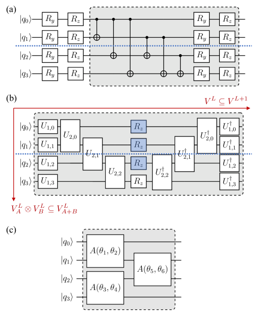
Figure 1: Heuristically designed HEA and physics-constrained HEA. (a) $R_{y}R_{z}$ full (EfficientSU2) ansatz. The $R_{y}$ full ansatz can be obtained by removing the columns of $R_{z}$ gates, while the $R_{y}$ linear ansatz can be derived from the $R_{y}$ full ansatz by further replacing the all-to-all CNOT gates by nearest neighbor CNOT gates. (b) XYZ1F (gates in white) and XYZ2F (gates in white and blue) ansätze. The dashed box indicates a single repeating unit $U_{l}(\vec{\theta}_{l})$, and all the parameters are omitted for brevity. The two inclusion constraints $V^{L}\subseteq V^{L+1}$ and $V^{L}_{A}\otimes V^{L}_{B}\subseteq V_{A+B}^{L}$ for extending HEA in different directions of quantum circuits are highlighted. The blue dashed line represents a partition of the whole system into two subsystems $A$ and $B$. (c) An example of particle-number conserving ansatz introduced in Refs. ^{57, 58}.

Some previously designed HEA are shown in Fig. 1a. The commonly used $R_{y}$ and $R_{y}R_{z}$ (EfficientSU2) ansätze with different entangling blocks⁴² clearly fail to meet these important requirements, in particular, constraints (2) and (3). It is obvious that the $R_{y}$ ansatz can only represent real wavefunctions, whereas it is unclear whether the $R_{y}R_{z}$ ansatz is universal. Recently, a ’cascade’ ansatz is developed to satisfy the condition $U_{l}(\vec{\theta}_{l})=I$ by adding the inverse of the CNOT gates in $R_{y}$ ansatz into the repeating unit⁴⁶. But it fails to meet the constraints (3) and (4). The HVA for model systems of the form $U_{l}(\vec{\theta}_{l})=\prod_{k}e^{\mathbbm{i}\theta_{l,k}\hat{H}_{k}}$, where $\hat{H}_{k}$ is a component of the Hamiltonian of the system $\hat{H}=\sum_{k}\hat{H}_{k}$, satisfies constraints (2) and (3), but does not necessarily meet constraints (1) and (4), which are requirements for general-purpose HEA. Similarly, the separable-pair approximation (SPA) ansatz^{59, 60} satisfies the size-consistency and is hardware-efficient, but not universal. Particle-number symmetry-preserving ansätze have also been introduced. A typical example is the ASWAP ansatz^{57, 58} shown in Fig. 1c, where the following exchange-type two-qubit gate $A(\theta,\phi)$ is used

$$A(\theta,\phi)=\begin{bmatrix}1&0&0&0\\ 0&\mathrm{cos}\ \theta&e^{\mathbbm{i}\phi}\mathrm{sin}\ \theta&0\\ 0&e^{-\mathbbm{i}\phi}\mathrm{sin}\ \theta&-\mathrm{cos}\ \theta&0\\ 0&0&0&1\end{bmatrix}.$$ (2)

Since only $|01\rangle$ and $|10\rangle$ are allowed to mix, this gate preserve the particle number of the input state with well-defined particle number. It is universal only within the Hilbert space with fixed number of electrons, but fails to satisfy the constraints (2) and (3), because the identity operator cannot be achieved by $A(\theta,\phi)$. The ansatz using the following hop gate⁶¹

$$h(\varphi)=\begin{bmatrix}1&0&0&0\\ 0&\cos\varphi&-\sin\varphi&0\\ 0&\sin\varphi&\cos\varphi&0\\ 0&0&0&-1\end{bmatrix}$$ (3)

also fails to satisfy the systematically improvability and size-consistency due to the exactly same problem. In summary, to the best of our knowledge, an HEA satisfying all these constraints has not been proposed before. Our goal is to design an HEA satisfying these constraints and hence it will not be particle number conserving in order to be universal, which is advantageous in applications such as computing Green’s functions^{62, 63}. For applications where the particle number is conserved, such as computing the ground state of molecules, we can apply penalties to enforce the correct particle numbers if necessary (vide post). Finally, we emphasize that apart from these theoretical constraints, since most of existing quantum devices have very restricted qubit connectivity, an additional important hardware constraint is that the building block $U_{l}(\vec{\theta}_{l})$ should be easily implemented on quantum devices with restricted connectivity.

2.2 Physics-constrained HEA

The above requirements still leave a lot of degree of freedom in the design of HEA. Here we propose one possible HEA that satisfies these basic requirements, referred as physics-constrained HEA, and only requires linear qubit connectivity. It should be pointed out that such realization of physics-constrained HEA is not unique, and other realizations are certainly possible, which is a subject of future investigations. Our starting point is the wavefunction given by a product of exponential of Pauli operators

$$|\Psi\rangle=e^{\mathbbm{i}\theta_{L}P_{L}}\cdots e^{\mathbbm{i}\theta_{1}P_{1}}|\Phi_{0}\rangle\triangleq\prod_{l=1}^{L}e^{\mathbbm{i}\theta_{l}P_{l}}|\Phi_{0}\rangle,$$ (4)

which is the form for the UCC type ansatz. A simple observation is that if one can choose all possible $P_{l}\in\{I,X,Y,Z\}^{\otimes N}$, this form of $U_{l}(\theta_{l})$ (= $e^{\mathbbm{i}\theta_{l}P_{l}}$) is universal^{64, 65}. It is also systematically improvable because the choice $\theta_{l}=0$ gives an identity operator. However, it does not satisfy constraints (3) and (4). Thus, if each layer of HEA has the ability to represent any $e^{\mathbbm{i}\theta_{l}P_{l}}$ with $P_{l}\in\{I,X,Y,Z\}^{\otimes N}$, the resulting ansatz will automatically satisfy constraints (1) and (2), and we only need to modify it to satisfy constraints (3) and (4). The fact that any $e^{\mathbbm{i}\theta_{l}P_{l}}$ can be represented by a quantum circuit with CNOT ’staircases’⁶⁴ (see Figs. 2a and 2b) motivates us to design $U_{l}(\vec{\theta}_{l})$ with a similar structure (see Fig. 2c), where the forms of the single-qubit gates $U_{1}$ and two-qubit gates $U_{2}$ remain to be specified. We find the following sufficient condition for representing any $e^{\mathbbm{i}\theta_{l}P_{l}}$ by the circuit block in Fig. 2c:

Theorem 1

If $U_{2}$ include gates in $\{I,\mathrm{CNOT},\mathrm{SWAP\;or\;iSWAP}\}$, then the circuit block in Fig. 2c can represent any $e^{\mathbbm{i}\theta_{l}P_{l}}$ with $P_{l}\in\{I,Z\}^{\otimes N}$. Furthermore, if $U_{1}$ include gates in $\{I,R_{x}(\pi/2),R_{y}(-\pi/2)\mathrm{\;or\;}H\}$, then the circuit block can represent any $e^{\mathbbm{i}\theta_{l}P_{l}}$ with $P_{l}\in\{I,X,Y,Z\}^{\otimes N}$.

The proof of Theorem 1 is quite straightforward. We only give two concrete examples in Fig. 2, arsing from the double excitation $a_{0}^{\dagger}a_{2}^{\dagger}a_{4}a_{5}$ and the single excitation $a_{1}^{\dagger}a_{4}$ in UCC, respectively. It can be easily verified that $e^{\mathbbm{i}\theta Z_{0}Z_{1}Z_{2}Z_{4}Z_{5}}$ in Fig. 2a is given by XYZ1F in Fig. 2c with $U_{2,k}=\mathrm{CNOT}$ for $k\in\{0,1,3,4\}$ and $U_{2,2}=\mathrm{SWAP}/\mathrm{iSWAP}$, while $e^{\mathbbm{i}\theta Z_{1}Z_{2}Z_{3}Z_{4}}$ in Fig. 2b is given by $U_{2,0}=I$, $U_{2,k}=\mathrm{CNOT}$ for $k\in\{1,2,3\}$, and $U_{2,4}=\mathrm{SWAP/\mathrm{iSWAP}}$. Other $e^{\mathbbm{i}\theta P_{l}}$ can be represented by a similar recipe. The role of $\mathrm{SWAP}$ can be replaced by $\mathrm{iSWAP}$, which is easier to implement on some quantum computing platforms, such as superconducting quantum devices⁶⁶.

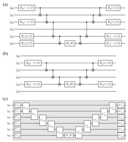
Figure 2: Examples for Theorem 1 with six qubits. (a), (b) quantum circuits appeared in UCC arising from the double excitation $a_{0}^{\dagger}a_{2}^{\dagger}a_{4}a_{5}$ and the single excitation $a_{1}^{\dagger}a_{4}$, respectively; (c) the XYZ1F circuit. Both (a) and (b) can be represented by (c) by appropriately choosing single-qubit gates $U_{1,k}$ from $\{I,R_{x}(\pi/2),R_{y}(-\pi/2)\mathrm{\;or\;}H\}$ and two-qubit gates $U_{2,k}$ from $\{I,\mathrm{CNOT},\mathrm{SWAP\;or\;iSWAP}\}$.

There are still infinitely many ways to parameterize $U_{1}$ and $U_{2}$ that satisfy this sufficient condition, since a general single-qubit (two-qubit) gate can be described by three (fifteen) parameters, and at most three CNOT gates are needed for general two-qubit gates^{67, 68}. To minimize the number of parameters per circuit block and reduce the number of native two-qubit gates in $U_{2}$, here we present a parameterization of $U_{2}$ with two parameters

$$U_{2}(\theta,\phi)=[I\otimes R_{y}(\phi/2)]U_{\mathrm{fSim}}(\theta,\phi)[I\otimes R_{y}(-\phi/2)],$$ (5)

using the fSim gate $U_{\mathrm{fSim}}(\theta,\phi)$ native on some superconducting devices⁶⁹

$$U_{\mathrm{fSim}}(\theta,\phi)=\begin{bmatrix}1&0&0&0\\ 0&\cos\theta&-\mathbbm{i}\sin\theta&0\\ 0&-\mathbbm{i}\sin\theta&\cos\theta&0\\ 0&0&0&e^{-\mathbbm{i}\phi}\\ \end{bmatrix},$$ (6)

which yields

$$U_{2}(0,0)=I,\quad U_{2}(-\pi/2,0)=\mathrm{iSWAP},\quad U_{2}(0,\pi)=\mathrm{CNOT}.$$ (7)

A simple choice for the single-qubit gates $U_{1}$ to satisfy the sufficient condition is

$$U_{1}(\theta,\phi)=R_{x}(\theta)R_{y}(\phi).$$ (8)

Eqs. (5) and (8) completely define a HEA, which can implement an exponential of any Pauli operator by appropriate choice of parameters. We will refer to it as XYZ1F in the following context, see Fig. 2c, as an abbreviation for the combination of the three types of single-qubit rotation gates used and the two-qubit gates involving fSim gates.

It is easy to see that the XYZ1F ansatz, however, does not yet satisfy constraint (3) and (4). Fortunately, by simply replacing the single $R_{z}$ gate in the middle by a layer of $R_{z}$ gate, we can resolve this problem and obtain the final physics-constrained HEA, denoted by XYZ2F in Fig. 1b (with additional gates in blue). The size-consistency of XYZ2F can be seen as follows: Suppose the subsystems $A$ and $B$ contain the first two and the remaining two qubits, respectively, then the wavefunction $|\Psi_{A}^{L}\rangle|\Psi_{B}^{L}\rangle$ formed by a direct product of the two XYZ2F wavefunctions can be represented by an XYZ2F ansatz for the composite system with $U_{2,1}=I$ (see Fig. 1b). Therefore, the ability of $U_{2}$ to become identity is essential from a size-consistent perspective, which is missing in other HEA shown in Figs. 1a and 1c. It can be verified that the constraint (4) is also satisfied by simply setting all $U_{2}$ to identity, such that for the $n$-th qubit the circuit block gives a universal single-qubit gate⁶⁴

$$U=R_{x}(\theta_{0})R_{y}(\theta_{1})R_{z}(\theta_{2})R_{y}^{\dagger}(\theta_{1})R_{x}^{\dagger}(\theta_{0}).$$ (9)

Another advantage of the size-consistent modification is that terms such as $e^{\mathbbm{i}(\theta_{1}X_{0}X_{1}+\theta_{2}X_{2}Z_{3}Z_{4}+\theta_{3}Y_{5})}$ can be implemented by a single layer in XYZ2F. In contrast, $e^{\mathbbm{i}\theta_{1}X_{0}X_{1}}e^{\mathbbm{i}\theta_{2}X_{2}Z_{3}Z_{4}}e^{\mathbbm{i}\theta_{3}Y_{5}}$ needs to be implemented by three consecutive blocks in XYZ1F. This will greatly reduce the number of layers required to represent certain states, as will be shown numerically for the ground state of the Heisenberg model and some typical molecules.

In summary, the constructed XYZ2F ansatz satisfies all the four fundamental constraints. The number of parameters in one layer of XYZ2F is $(5N-2)$, where $3N$ and $2(N-1)$ are for single-qubit and two-qubit gates, respectively. Comparing the exponential $e^{\mathbbm{i}\theta_{l}P_{l}}$ with $P_{l}\in\{I,X,Y,Z\}^{\otimes N}$, it is seen that all the $4^{N}$ discrete choices of $P_{l}$ are now embedded into a continuous space of operators $U_{l}(\vec{\theta}_{l})$ specified by $O(N)$ parameters. Therefore, it can be viewed as an adaptive ansatz, where the operator pool contains all $4^{N}$ Pauli operators rather than given by UCCSD as in other adaptive methods^{35, 36, 37, 38}. In Table 1, we compare different HEA in terms of the numbers of parameters $N_{\mathrm{param}}$, two-qubit gates $N_{2}$, single-qubit gates $N_{1}$, and the circuit depth $D$ as a function of the layer $L$ and the number of qubits $N$. The number of parameters in all of them scales as $O(NL)$. One disadvantage of XYZ1F and XYZ2F is that the circuit depths of XYZ1F and XYZ2F is larger than other HEA due to the use of the staircase structure. In principle, other low-depth architectures such as the brickwall structure can be used in the construction of physics-constrained HEA. We are exploring such possibility and the results will be reported elsewhere.

Table 1: Comparison of different HEA in terms of the numbers of parameters $N_{\mathrm{param}}$, two-qubit gates $N_{2}$, single-qubit gates $N_{1}$, and the circuit depth $D$ as a function of the layer $L$ and the number of qubits $N$. When counting $N_{2}$ and $D$, we assume the ASWAP and fSim gates are native gates.

ansatz	$N_{\mathrm{param}}$	$N_{2}$	$N_{1}$	$D$ ($N\geq 3,L\geq 1$)
$R_{y}$ linear	$N(L+1)$	$(N-1)L$	$N(L+1)$	$N+3L-2$
$R_{y}$ full	$N(L+1)$	$N(N-1)L/2$	$N(L+1)$	$NL+N+L-2$
$R_{y}R_{z}$ full	$2N(L+1)$	$N(N-1)L/2$	$2N(L+1)$	$NL+N+2L-2$
ASWAP	$2(N-1)L$	$(N-1)L$	0	$2L$
XYZ1F	$(4N-1)L$	$2(N-1)L$	$(8N-3)L$	$(4N+3)L$
XYZ2F	$(5N-2)L$	$2(N-1)L$	$(9N-4)L$	$(4N+3)L$

2.3 Layerwise optimization algorithm

To take full advantage of the systematic improvability of XYZ1F and XYZ2F, the parameters in HEA are optimized in a layerwise way using the Algorithm 1. This is different from optimization with random initialization for all parameters, which has been shown to easily suffer from the problems of low-quality local minima and barren plateaus⁴⁵. Our algorithm has two key features. First, we retain the optimized parameters from the previous step as the initial guess for the $L-1$ layers in the current step. Second, we generate $n$ (about 10) sets of random parameters with different step sizes for the $L$-th layer. Each set of parameters $\vec{\theta}_{L}$ is obtained from $\vec{\theta}_{L}=\frac{\vec{u}}{\max_{i}|u_{i}|}\delta$, where $\vec{u}$ are random numbers in $[-1,1]$ and $\delta$ is a predefined step size $\delta\in\{\frac{2\pi}{2^{k}}\}_{k=0}^{5}\cup\{0\}$. This guarantees that the optimized energy decreases monotonically with respect to $L$ for XYZ1F and XYZ2F. For consistency, the layerwise optimization method is also employed in calculations using other HEA. We implement all the HEA using MindQuantum⁷⁰. Numerical optimization in VQE employed the Broyden–Fletcher–Goldfarb–Shanno (BFGS) method implemented in Scipy⁷¹. As shown in the Supplementary Materials, during the the optimization, the decrease of the energy is fast at the beginning of iterations and then slows down. Thus, we set the maximal number of iterations to be 3000 for a given layer.

Algorithm 1 Layerwise optimization strategy

$L_{\max}$, $|\Phi_{0}\rangle$;

Initialization: $L=0,|\Psi\rangle=|\Phi_{0}\rangle$;

while $L\leq L_{\max}$ do

     Set $L\mathrel{+}=1$;

     Generate $n$ sets of random parameters $\{\vec{\theta}_{L}^{(i)}\}_{i=1}^{n}$ with different step sizes for the $L$-th layer;

     Combine $\{\vec{\theta}_{1},\dots,\vec{\theta}_{L-1}\}$ obtained in the previous step as initial guess for the $L-1$ layers;

     Perform $n$ independent VQE with $|\Psi\rangle=U_{L}\cdots U_{1}|\Phi_{0}\rangle$ in parallel;

     Collect $E_{L}=\min_{i}E^{(i)}_{L}$ and optimized $\{\vec{\theta}_{1},\dots,\vec{\theta}_{L}\}$;

end while

$\{E_{1},\cdots,E_{L_{\max}}\}$ and $|\Psi\rangle=U_{L_{\max}}\cdots U_{1}|\Phi_{0}\rangle$.

Figure 3 displays the variance of energy gradients for the one-dimensional Heisenberg model (see the next section). We observe the exponential vanishing of gradients with respect to the number of qubits $N$ and the number of layers $L$ with random initialization, consistent with the conclusions in Ref. ⁴⁵. In contrast, the layerwise optimization alleviates the barren plateau problem in particular for XYZ2F.

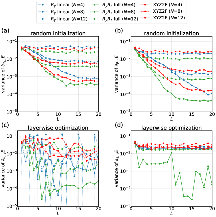
Figure 3: Variance of energy gradients for the one-dimensional Heisenberg model. (a) and (b): the variances of energy gradients for the first parameter in the first layer $\theta_{1,1}$ and that in the $L$-th layer $\theta_{L,1}$ are computed with random initialization of all parameters for 500 times. For all the HEA, an exponential vanishing of gradients with respect to the number of qubits $N$ and the number of layers $L$ are observed, consistent with the conclusions in Ref. ⁴⁵. (c) and (d): instead of random initialization, the parameters for the previous $L-1$ layers are the optimized parameters, while those for the $L$-th layer are initialized randomly for 500 times. Compared with random initialization, the layerwise optimization alleviates the barren plateau problem.

3 Results

3.1 Heisenberg model

We first use the one-dimensional Heisenberg model with open boundary condition, whose Hamiltonian is $\hat{H}=-\frac{1}{2}J\sum_{n=1}^{N-1}\vec{\sigma}_{n}\cdot\vec{\sigma}_{n+1}$, to study the effectiveness of the constructed HEA. In Table 2, we perform a size-consistent test^{54, 56} for different HEA by applying them to a composite Heisenberg model (denoted by 6+6) consisting of two noninteracting subsystems with six sites. The parameters in the wavefunction of the composite system are taken from the optimized parameters for the subsystem. If an ansatz is size-consistent, then the ground-state energy per site $e_{N}^{L}$ should be the same for the whole system and the subsystem, i.e. $e_{6+6}^{L}=e_{6}^{L}$ for any $L$. Notably, only XYZ2F satisfies this condition, while other HEA violate it significantly. The additional entangling gates between subsystems in other HEA severely degrade the quality of the approximation in the total system, as can be seen from the significant increase of infidelity ($1-F_{N}^{L}$ with $F_{N}^{L}=|\langle\Psi_{N}^{L}|\Psi_{N}^{*}\rangle|^{2}$, where $|\Psi_{N}^{*}\rangle$ is the exact wavefunction) in Table 2. In particular, the additional CNOT gates in the $R_{y}$ full ansatz (see Fig. 1a) makes the fidelity between the approximate state and the ground state almost vanish. On the contrary, the infidelity for XYZ2F is well-controlled, that is, if the fidelity $F_{6}^{L}$ is $1-\epsilon$, where $\epsilon$ is a small number (0.00085 for $L=2$ in Table 2), then the fidelity for the total system is $(1-\epsilon)^{2}$, and thus the infidelity $1-F_{6+6}^{L}$ is about $2\epsilon$. Therefore, an interesting topic for future studies is to use parameters optimized from small systems as an initial guess of XYZ2F for large systems.

Table 2: Size-consistency test: ground-state energy per site $e_{N}^{L}$ and infidelities ($1-F_{N}^{L}$ with $F_{N}^{L}=|\langle\Psi_{N}^{L}|\Psi_{N}^{*}\rangle|^{2}$) obtained by different HEA with $L=2$ and $L=4$ for a composite Heisenberg model (denoted by 6+6), which consists of two noninteracting subsystems with six sites. The parameters of the total system are taken from the optimized parameters of the subsystems. Errors with respect to the exact $e_{N}^{*}$ obtained from exact diagonalization are shown in parenthesis. Only XYZ2F satisfies $e_{6+6}^{L}=e_{6}^{L}$, while other HEA are not size-consistent.

system	$R_{y}$ linear	$R_{y}$ full	$R_{y}R_{z}$ full	ASWAP	XYZ2F
$e_{6}^{L=2}$	-0.78333	-0.78333	-0.80606	-0.80273	-0.83054
	(0.04786)	(0.04786)	(0.02514)	(0.02846)	(0.00065)
$e_{6+6}^{L=2}$	-0.52002	-0.51368	-0.64791	-0.52267	-0.83054
	(0.31118)	(0.31751)	(0.18328)	(0.30853)	(0.00065)
$e_{6}^{L=4}$	-0.82988	-0.82988	-0.83089	-0.83119	-0.83119
	(0.00132)	(0.00132)	(0.00030)	(0.00000)	(0.00000)
$e_{6+6}^{L=4}$	-0.33247	-0.35020	-0.53154	-0.63073	-0.83119
	(0.49873)	(0.48099)	(0.29966)	(0.20047)	(0.00000)
$1-F_{6}^{L=2}$	0.17623	0.17623	0.03743	0.05260	0.00085
$1-F_{6+6}^{L=2}$	0.77773	1.00000	1.00000	0.95358	0.00170
$1-F_{6}^{L=4}$	0.00205	0.00205	0.00037	0.00000	0.00000
$1-F_{6+6}^{L=4}$	0.93368	1.00000	0.93196	0.79871	0.00000

Figure 4 shows the convergence of the ground-state energy per site $e_{N}^{L}$ obtained by different HEA for antiferromagnetic Heisenberg models as a function of the number of layers $L$ starting from a Néel state as reference $|\Phi_{0}\rangle$. We find that both XYZ1F and XYZ2F are systematically improvable as expected, and the effect of the size-consistent modification in XYZ2F is dramatic, which significantly reduces the number of layers needed to reach certain accuracy. In contrast, other HEA do not converge monotonically and become increasingly difficult to converge as the system size $N$ increases (except for ASWAP). As shown in Fig. 4, the oscillatory behavior reveals a severe problem of these HEA in practical applications, that is, even if they have reached a certain accuracy with $L$ layers, the accuracy with $L+1$ layers may be worse. The comparison with XYZ1F/XYZ2F suggests that it is the violation of constraints (2) and (3) that causes these heuristically designed HEA to perform poorly as $N$ increases.

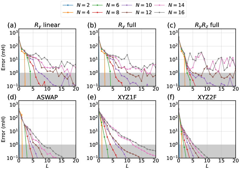
Figure 4: Convergence of the ground-state energy per site $e_{N}^{L}$ obtained by different HEA ($R_{y}$ linear, $R_{y}$ full, $R_{y}R_{z}$ full, ASWAP, XYZ1F and XYZ2F) as a function of the number of layers $L$ for one-dimensional antiferromagnetic Heisenberg models ($J=-1$) with different number of sites $N$. The exact values $e_{N}^{*}$ are obtained from exact diagonalizations. While both XYZ1F and XYZ2F are systematically improvable, the size-consistency of XYZ2F makes it superior to XYZ1F. Other HEA do not converge monotonically, and become increasingly difficult to achieve a target accuracy as the system size increases (except for ASWAP). The shaded regions represent the region within the chemical accuracy (1 mH).

In Fig. 5a, we display the number of variational parameters $N_{\mathrm{param}}$ to reach 1 milli-Hartree as a function of the number of sites $N$, compared against the dimension of the Hilbert space $\binom{N}{N/2}$ for different $N$. It is seen that for this system, the number of variational parameters to reach 1 milli-Hartree scales as $O(N^{1.98})$ for XYZ2F. The scaling for XYZ1F and ASWAP are quite similar, but the ASWAP has a much smaller prefactor. Figure 5b shows the scaling of the number of two-qubit gates $N_{2}$ required to reach 1 milli-Hatree for different $N$. It is seen that XYZ2F has the lowest scaling $O(N^{2.17})$, albeit with a larger prefactor than ASWAP. Therefore, future optimization of the layout may further lead to more economic physics-constrained HEA.

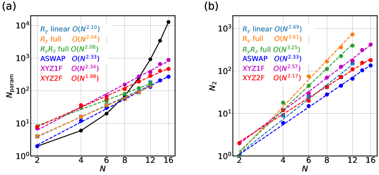
Figure 5: The number of variational parameters $N_{\mathrm{param}}$ (a) and the number of two-qubit gates $N_{2}$ (b) required to reach 1 milli-Hartree as a function of the number of sites $N$ for one-dimensional antiferromagnetic Heisenberg models ($J=-1$). The dimension of the Hilbert space $\binom{N}{N/2}$ for different $N$ is shown for comparison. The fitted scaling $O(N^{b})$ is shown by dashed lines.

3.2 Molecules

Next we examine the performance of the constructed HEA for realistic systems. For molecules, the molecular integrals were generated using the PySCF package⁷² in a minimal STO-3G basis. The Jordan-Wigner fermion-to-qubit transformation⁷³ was carried out using OpenFermion⁷⁴, where occupation number vectors (ONVs) for fermions $|n_{0}n_{\bar{0}}n_{1}n_{\bar{1}}\cdots n_{k}n_{\bar{k}}\rangle$ ($n\in\{0,1\}$ and the symbol $\bar{i}$ represents $i$-th $\beta$ spin-orbital) is mapped to ONVs for qubits $|q_{0}q_{1}q_{2}q_{3}\cdots q_{2k-1}q_{2k}\rangle$.

Table 3 shows the size-consistency test for a composite hydrogen ladder composed of two H4 chain ($R_{\mathrm{H-H}}=$1.5 Å) separated by a distance of 100 Å. It is well-known that classical spin-restricted coupled cluster singles and doubles (CCSD) is size-consistent/extensive in this case. However, it is seen that the commonly used Trotterized unitary CCSD (UCCSD) using the canonical molecular orbitals (CMO) has a small size-consistency error. Here, we only consider a single Trotter step. The Trotterization makes UCCSD lose the property of orbital invariance. Since the CMO of the H4 ladder, which is delocalized among all hydrogen, is different from that of the H4 monomer, the UCCSD wavefunction cannot be exactly factorized into a product of two wavefunctions. The Trotterized UCCSD can become size-consistent only with localized molecular orbitals (LMO) with a proper ordering of qubits. Similarly, we can only expect size-consistency for HEA using localized orbitals. Table 3 shown the results obtained with $L=6$ using orthonormalized atomic orbitals (OAO). It is clear that only XYZ2F is size-consistent in this case.

Table 3: Size-consistency test for a composite system composed of two H4 chains ($R_{\mathrm{H-H}}=$1.5 Å) separated by a distance of 100 Å. The ground-state energies for the monomer and the entire system are obtained by classical coupled cluster singles and doubles (CCSD) and single-step Trotterized unitary CCSD (UCCSD) using canonical molecular orbitals (CMO). For HEA, the results are obtained with $L=6$ using orthonormalized atomic orbitals (OAO). The optimized parameters for H4 are taken as the parameters for the H4-H4 ladder. Errors with respect to the FCI are shown in parenthesis.

system	CCSD	UCCSD	$R_{y}$ linear	$R_{y}$ full	$R_{y}R_{z}$ full	ASWAP	XYZ2F
	(CMO)	(CMO)	(OAO)	(OAO)	(OAO)	(OAO)	(OAO)
$E_{\mathrm{H_{4}}}$	-1.99762	-1.99460	-1.97672	-1.99045	-0.92429	-1.99113	-1.99560
	(-0.00147)	(0.00155)	(0.01943)	(0.00570)	(1.07186)	(0.00502)	(0.00055)
$E_{\mathrm{H_{4}\textnormal{-}H_{4}}}$	-3.99525	-3.98918	-2.52810	-2.36808	-1.85371	-3.48508	-3.99119
	(-0.00295)	(0.00312)	(1.46420)	(1.62422)	(2.13859)	(0.50722)	(0.00111)
$E_{\mathrm{H_{4}\textnormal{-}H_{4}}}-2E_{\mathrm{H_{4}}}$	0	2.3$\times 10^{-5}$	1.43	1.61	-5.1$\times 10^{-3}$	$5.0\times 10^{-1}$	0

Figure 6 shows the comparison of different HEA for the convergence of ground-state energies as a function of the number of layers $L$ for hydrogen chains (H4, H6, and H8), LiH, H2O, and N2, which were commonly used to benchmark the performance of quantum computing techniques^{42, 33, 46, 75, 76}. For the stretched hydrogen chains, the OAO were used due to the faster convergence and the reference state was a Néel state, e.g. $|\Phi_{0}\rangle=|10011001\rangle$ for H4. As the number of hydrogen increases, the number of Slater determinants with large coefficients in the expansion of the exact ground state increases significantly. As shown in Fig. 6, only XYZ2F converges monotonically to chemical accuracy, while other HEA perform poorly for H6 and H8. The number of layers needed to achieve chemical accuracy increases roughly linearly with the system size for XYZ2F.

For LiH, H2O, and N2, all simulated with 12 qubits using the restricted Hartree-Fock (RHF) orbitals, the convergence behavior is quite different, reflecting the very different electronic structures. For LiH at $R_{\mathrm{Li\textnormal{-}H}}=2.0$ Å, the exact ground state is dominated by the Hartree-Fock configuration (about 95%), and thus XYZ2F quickly reaches chemical accuracy with $L=3$. For H2O and N2 at stretched geometries upon dissociation, which are typical examples of strong electron correlations in quantum chemistry, the convergence is slower. In the calculation of H2O, we added a penalty term for preserving the particle number, viz. $\hat{H}^{\prime}=\hat{H}+\beta(\hat{N}_{\uparrow}-n_{\uparrow})^{2}+\beta(\hat{N}_{\downarrow}-n_{\downarrow})^{2}$ with $\beta=1.0$. In the calculations of N2, we further added a penalty for the total spin, viz. $\hat{H}^{\prime}=\hat{H}+\beta(\hat{N}_{\uparrow}-n_{\uparrow})^{2}+\beta(\hat{N}_{\downarrow}-n_{\downarrow})^{2}+\beta\hat{S}_{+}\hat{S}_{-}$ with $\beta=1.0$. For the ASWAP ansatz, a larger $\beta=3.0$ is used, otherwise it will not converge to the ground state. As shown in Fig. 6, the number of layers required for XYZ2F to reach chemical accuracy is 11 and 27, respectively. For the most challenging molecule N2, we find that other HEA are difficult to converge to chemical accuracy.

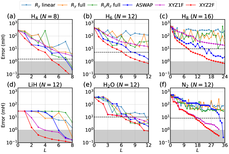
Figure 6: Ground-state energy convergence with respect to exact diagonalization results as a function of the number of layers $L$ for molecules: (a)-(c) hydrogen chains (H₄, H₆, and H₈) with interatomic distance $R_{\mathrm{H\textnormal{-}H}}=1.5$ Å; (d) LiH ($R_{\mathrm{Li\textnormal{-}H}}=2.0$ Å); (e) H₂O ($R_{\mathrm{O\textnormal{-}H}}=2.0$ Å and $\theta_{\mathrm{H\textnormal{-}O\textnormal{-}H}}=104.5$ degree); (f) N₂ ($R_{\mathrm{N\textnormal{-}N}}=2.0$ Å). For H2O, the O1s orbital is frozen, while the N1s and N2s orbitals are frozen for N2. The black dashed lines represent UCCSD results, while the shaded regions represent the region within the chemical accuracy (1 mH).

Finally, we test the performance of HEA on a more challenging two-dimensional system, a H3-H3 ladder (see Fig. 7). We should mention that $R_{y}$ linear, ASWAP, XYZ1F, and XYZ2F are designed to be one-dimensional, and we are working on the two-dimensional extensions. But we can examine their performance on a two-dimensional system. The convergence of different HEA for the ground-state energy at three representative distances (0.7 Å, 1.5 Å, and 3.0 Å) are shown in Fig. 7. Both in the equilibrium ($d=0.7$ Å) and in the dissociation region ($d=3.0$ Å), XYZ2F converge to the chemical accuracy easily, because the systems can be viewed as close to three hydrogen molecules and two H3, respectively. At $d=$1.5 Å, which equals to $R_{\mathrm{H\textnormal{-}H}}$ within the monomer, the system is most difficult. We find that XYZ2F require about 37 layers to converge to the chemical accuracy, while XYZ1F and ASWAP converge much more slowly. Other HEA completely fail. It is seen that ensuring the universality, systematical improvability, and size-consistency is important for the good performance of HEA even in this challenging case. Therefore, we expect that by extending the physics-constrained HEA to two-dimensional systems, better performance can be obtained.

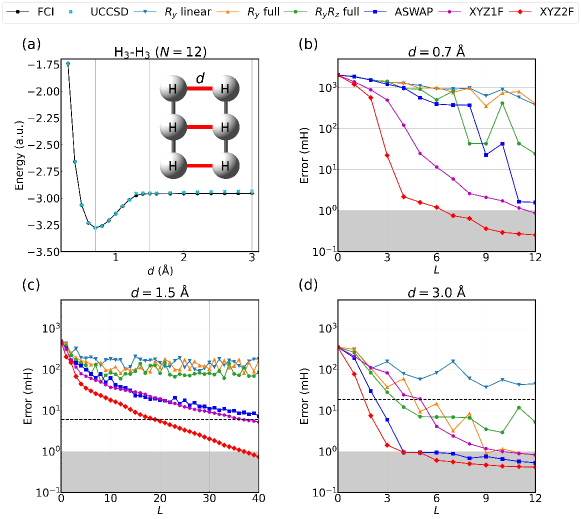
Figure 7: A two-dimensional ladder H3-H3 where $R_{\mathrm{H\textnormal{-}H}}=1.5$ Å within each monomer. (a) Potential energy curve described by full configuration interaction (FCI) and unitary CCSD (UCCSD). Note that the performance of UCCSD deteriorates as $d$ exceeds 1.3 Å. (b)-(d) Convergence of different HEA for the ground-state energy at three representative distances (0.7 Å, 1.5 Å, and 3.0 Å). The black dashed lines represent UCCSD results. The error of UCCSD at $d=0.7$ Å is below 1 micro-Hartree.

4 Conclusion

In this work, we introduced a new way to design HEA by satisfying fundamental constraints, inspired by the physics-constrained way to design non-empirical XC functionals in DFT⁴⁸. The developed physics-constrained HEA - XYZ2F is superior to other heuristically designed HEA in terms of both accuracy and scalability. In particular, numerical tests show the promise of XYZ2F for challenging realistic molecules with strong electron correlation. The better scalability of XYZ2F is attributed to the satisfaction of the systematic improvability and size-consistency. Our results suggest that incorporating physical constraints into the design of HEA is a promising path towards designing efficient variational ansätze for solving many-body problems on quantum computers.

One disadvantage of XYZ2F is its high circuit depth, due to the use of the staircase structure. This stems from the requirement that the circuit block can represent any exponential of a Pauli operator, which is a sufficient condition for the universality. However, this is not a necessary condition, other conditions for the universality can be imposed, which may lead to lower circuit depth. Another very interesting direction is that while we only consider one-dimensional HEA in this work, the concepts of physics-constrained HEA can be extended to construct HEA for higher dimensions. We are exploring these directions. It is conceivable that this work will inspire other realizations of HEA that satisfy these basic constraints, probably with more interesting properties such as less parameters, faster convergence, better trainability, and more versatile qubit connectivity.

The authors acknowledge helpful comments by Jakob Kottmann and Mario Motta. This work was supported by the National Natural Science Foundation of China (Grants No. 21973003) and the Fundamental Research Funds for the Central Universities.

Additional information including the energy convergence behavior of XYZ2F, the convergence with respect to the number of parameters, two-qubit gates count, and circuit depth, comparison of the use of different orbitals and references, and results obtained from noisy simulations.

This information is available free of charge via the Internet at http://pubs.acs.org.

References

- Martin et al. 2016 Martin, R. M.; Reining, L.; Ceperley, D. M. Interacting electrons; Cambridge University Press, 2016
- Gutzwiller 1963 Gutzwiller, M. C. Effect of correlation on the ferromagnetism of transition metals. Phys. Rev. Lett. 1963, 10, 159
- Jastrow 1955 Jastrow, R. Many-body problem with strong forces. Phys. Rev. 1955, 98, 1479
- White 1992 White, S. R. Density matrix formulation for quantum renormalization groups. Phys. Rev. Lett. 1992, 69, 2863
- Verstraete and Cirac 2004 Verstraete, F.; Cirac, J. I. Renormalization algorithms for quantum-many body systems in two and higher dimensions. arXiv preprint cond-mat/0407066 2004,
- Shi et al. 2006 Shi, Y.-Y.; Duan, L.-M.; Vidal, G. Classical simulation of quantum many-body systems with a tree tensor network. Phys. Rev. A 2006, 74, 022320
- Vidal 2008 Vidal, G. Class of quantum many-body states that can be efficiently simulated. Phys. Rev. Lett. 2008, 101, 110501
- Verstraete et al. 2008 Verstraete, F.; Murg, V.; Cirac, J. I. Matrix product states, projected entangled pair states, and variational renormalization group methods for quantum spin systems. Adv. Phys. 2008, 57, 143–224
- Schollwöck 2011 Schollwöck, U. The density-matrix renormalization group in the age of matrix product states. Ann. Phys. 2011, 326, 96–192
- Orús 2014 Orús, R. A practical introduction to tensor networks: Matrix product states and projected entangled pair states. Ann. Phys. 2014, 349, 117–158
- Carleo and Troyer 2017 Carleo, G.; Troyer, M. Solving the quantum many-body problem with artificial neural networks. Science 2017, 355, 602–606
- Choo et al. 2018 Choo, K.; Carleo, G.; Regnault, N.; Neupert, T. Symmetries and many-body excitations with neural-network quantum states. Phys. Rev. Lett. 2018, 121, 167204
- Liang et al. 2018 Liang, X.; Liu, W.-Y.; Lin, P.-Z.; Guo, G.-C.; Zhang, Y.-S.; He, L. Solving frustrated quantum many-particle models with convolutional neural networks. Phys. Rev. B 2018, 98, 104426
- Choo et al. 2019 Choo, K.; Neupert, T.; Carleo, G. Two-dimensional frustrated J 1- J 2 model studied with neural network quantum states. Phys. Rev. B 2019, 100, 125124
- Hibat-Allah et al. 2020 Hibat-Allah, M.; Ganahl, M.; Hayward, L. E.; Melko, R. G.; Carrasquilla, J. Recurrent neural network wave functions. Phys. Rev. Res. 2020, 2, 023358
- Sharir et al. 2020 Sharir, O.; Levine, Y.; Wies, N.; Carleo, G.; Shashua, A. Deep autoregressive models for the efficient variational simulation of many-body quantum systems. Phys. Rev. Lett. 2020, 124, 020503
- Barrett et al. 2022 Barrett, T. D.; Malyshev, A.; Lvovsky, A. Autoregressive neural-network wavefunctions for ab initio quantum chemistry. Nat. Mach. Intell. 2022, 4, 351–358
- Arute et al. 2019 Arute, F. et al. Quantum supremacy using a programmable superconducting processor. Nature 2019, 574, 505–510
- Wu et al. 2021 Wu, Y. et al. Strong Quantum Computational Advantage Using a Superconducting Quantum Processor. Phys. Rev. Lett. 2021, 127, 180501
- Peruzzo et al. 2014 Peruzzo, A.; McClean, J.; Shadbolt, P.; Yung, M.-H.; Zhou, X.-Q.; Love, P. J.; Aspuru-Guzik, A.; O’Brien, J. L. A variational eigenvalue solver on a photonic quantum processor. Nat. Commun. 2014, 5, 4213
- McClean et al. 2016 McClean, J. R.; Romero, J.; Babbush, R.; Aspuru-Guzik, A. The theory of variational hybrid quantum-classical algorithms. New J. Phys. 2016, 18, 023023
- Tilly et al. 2022 Tilly, J.; Chen, H.; Cao, S.; Picozzi, D.; Setia, K.; Li, Y.; Grant, E.; Wossnig, L.; Rungger, I.; Booth, G. H., et al. The variational quantum eigensolver: a review of methods and best practices. Phys. Rep. 2022, 986, 1–128
- Cao et al. 2019 Cao, Y.; Romero, J.; Olson, J. P.; Degroote, M.; Johnson, P. D.; Kieferová, M.; Kivlichan, I. D.; Menke, T.; Peropadre, B.; Sawaya, N. P.; Sim, S.; Veis, L.; Aspuru-Guzik, A. Quantum chemistry in the age of quantum computing. Chem. Rev. 2019, 119, 10856–10915
- McArdle et al. 2020 McArdle, S.; Endo, S.; Aspuru-Guzik, A.; Benjamin, S. C.; Yuan, X. Quantum computational chemistry. Rev. Mod. Phys. 2020, 92, 015003
- Bauer et al. 2020 Bauer, B.; Bravyi, S.; Motta, M.; Chan, G. K.-L. Quantum algorithms for quantum chemistry and quantum materials science. Chem. Rev. 2020, 120, 12685–12717
- Cerezo et al. 2021 Cerezo, M.; Arrasmith, A.; Babbush, R.; Benjamin, S. C.; Endo, S.; Fujii, K.; McClean, J. R.; Mitarai, K.; Yuan, X.; Cincio, L.; Coles, P. J. Variational quantum algorithms. Nat. Rev. Phys. 2021, 3, 625–644
- Anand et al. 2022 Anand, A.; Schleich, P.; Alperin-Lea, S.; Jensen, P. W.; Sim, S.; Díaz-Tinoco, M.; Kottmann, J. S.; Degroote, M.; Izmaylov, A. F.; Aspuru-Guzik, A. A quantum computing view on unitary coupled cluster theory. Chem. Soc. Rev. 2022,
- Bartlett and Musiał 2007 Bartlett, R. J.; Musiał, M. Coupled-cluster theory in quantum chemistry. Rev. Mod. Phys. 2007, 79, 291
- Preskill 2018 Preskill, J. Quantum Computing in the NISQ era and beyond. Quantum 2018, 2, 79
- Whitfield et al. 2011 Whitfield, J. D.; Biamonte, J.; Aspuru-Guzik, A. Simulation of electronic structure Hamiltonians using quantum computers. Mol. Phys. 2011, 109, 735–750
- Seeley et al. 2012 Seeley, J. T.; Richard, M. J.; Love, P. J. The Bravyi-Kitaev transformation for quantum computation of electronic structure. J. Chem. Phys. 2012, 137, 224109
- Hastings et al. 2015 Hastings, M. B.; Wecker, D.; Bauer, B.; Troyer, M. Improving quantum algorithms for quantum chemistry. Quantum Inf. Comput. 2015, 15, 1–21
- Lee et al. 2018 Lee, J.; Huggins, W. J.; Head-Gordon, M.; Whaley, K. B. Generalized unitary coupled cluster wave functions for quantum computation. J. Chem. Theory Comput. 2018, 15, 311–324
- Matsuzawa and Kurashige 2020 Matsuzawa, Y.; Kurashige, Y. Jastrow-type decomposition in quantum chemistry for low-depth quantum circuits. J. Chem. Theory Comput. 2020, 16, 944–952
- Ryabinkin et al. 2018 Ryabinkin, I. G.; Yen, T.-C.; Genin, S. N.; Izmaylov, A. F. Qubit coupled cluster method: a systematic approach to quantum chemistry on a quantum computer. J. Chem. Theory Comput. 2018, 14, 6317–6326
- Grimsley et al. 2019 Grimsley, H. R.; Economou, S. E.; Barnes, E.; Mayhall, N. J. An adaptive variational algorithm for exact molecular simulations on a quantum computer. Nat. Commun. 2019, 10, 3007
- Tang et al. 2021 Tang, H. L.; Shkolnikov, V.; Barron, G. S.; Grimsley, H. R.; Mayhall, N. J.; Barnes, E.; Economou, S. E. qubit-adapt-vqe: An adaptive algorithm for constructing hardware-efficient ansätze on a quantum processor. PRX Quantum 2021, 2, 020310
- Yordanov et al. 2021 Yordanov, Y. S.; Armaos, V.; Barnes, C. H.; Arvidsson-Shukur, D. R. Qubit-excitation-based adaptive variational quantum eigensolver. Commun. Phys. 2021, 4, 228
- Wecker et al. 2014 Wecker, D.; Bauer, B.; Clark, B. K.; Hastings, M. B.; Troyer, M. Gate-count estimates for performing quantum chemistry on small quantum computers. Phys. Rev. A 2014, 90, 022305
- Wecker et al. 2015 Wecker, D.; Hastings, M. B.; Troyer, M. Progress towards practical quantum variational algorithms. Phys. Rev. A 2015, 92, 042303
- Wiersema et al. 2020 Wiersema, R.; Zhou, C.; de Sereville, Y.; Carrasquilla, J. F.; Kim, Y. B.; Yuen, H. Exploring entanglement and optimization within the hamiltonian variational ansatz. PRX Quantum 2020, 1, 020319
- Kandala et al. 2017 Kandala, A.; Mezzacapo, A.; Temme, K.; Takita, M.; Brink, M.; Chow, J. M.; Gambetta, J. M. Hardware-efficient variational quantum eigensolver for small molecules and quantum magnets. Nature 2017, 549, 242
- Bittel and Kliesch 2021 Bittel, L.; Kliesch, M. Training variational quantum algorithms is np-hard. Phys. Rev. Lett. 2021, 127, 120502
- Anschuetz and Kiani 2022 Anschuetz, E. R.; Kiani, B. T. Quantum variational algorithms are swamped with traps. Nat. Commun. 2022, 13, 7760
- McClean et al. 2018 McClean, J. R.; Boixo, S.; Smelyanskiy, V. N.; Babbush, R.; Neven, H. Barren plateaus in quantum neural network training landscapes. Nat. Commun. 2018, 9, 1–6
- D’Cunha et al. 2023 D’Cunha, R.; Crawford, T. D.; Motta, M.; Rice, J. E. Challenges in the Use of Quantum Computing Hardware-Efficient Ansätze in Electronic Structure Theory. J. Phys. Chem. A 2023,
- Motta et al. 2023 Motta, M.; Sung, K. J.; Whaley, K. B.; Head-Gordon, M.; Shee, J. Bridging physical intuition and hardware efficiency for correlated electronic states: the local unitary cluster Jastrow ansatz for electronic structure. ChemRxiv preprint ChemRxiv:10.26434/chemrxiv-2023-d1b3l 2023,
- Kaplan et al. 2023 Kaplan, A. D.; Levy, M.; Perdew, J. P. The predictive power of exact constraints and appropriate norms in density functional theory. Annu. Rev. Phys. Chem. 2023, 74, 193–218
- Perdew et al. 1996 Perdew, J. P.; Burke, K.; Ernzerhof, M. Generalized gradient approximation made simple. Phys. Rev. Lett. 1996, 77, 3865
- Sun et al. 2015 Sun, J.; Ruzsinszky, A.; Perdew, J. P. Strongly constrained and appropriately normed semilocal density functional. Phys. Rev. Lett. 2015, 115, 036402
- Cybenko 1989 Cybenko, G. Approximation by superpositions of a sigmoidal function. Mathematics of control, signals and systems 1989, 2, 303–314
- Hornik et al. 1989 Hornik, K.; Stinchcombe, M.; White, H. Multilayer feedforward networks are universal approximators. Neural networks 1989, 2, 359–366
- He et al. 2016 He, K.; Zhang, X.; Ren, S.; Sun, J. Deep residual learning for image recognition. Proceedings of the IEEE conference on computer vision and pattern recognition. 2016; pp 770–778
- Pople et al. 1976 Pople, J. A.; Binkley, J. S.; Seeger, R. Theoretical models incorporating electron correlation. Int. J. Quantum Chem. 1976, 10, 1–19
- Bartlett 1981 Bartlett, R. J. Many-body perturbation theory and coupled cluster theory for electron correlation in molecules. Annu. Rev. Phys. Chem. 1981, 32, 359–401
- Nooijen et al. 2005 Nooijen, M.; Shamasundar, K.; Mukherjee, D. Reflections on size-extensivity, size-consistency and generalized extensivity in many-body theory. Mol. Phys. 2005, 103, 2277–2298
- Barkoutsos et al. 2018 Barkoutsos, P. K.; Gonthier, J. F.; Sokolov, I.; Moll, N.; Salis, G.; Fuhrer, A.; Ganzhorn, M.; Egger, D. J.; Troyer, M.; Mezzacapo, A., et al. Quantum algorithms for electronic structure calculations: Particle-hole hamiltonian and optimized wave-function expansions. Phys. Rev. A 2018, 98, 022322
- Gard et al. 2020 Gard, B. T.; Zhu, L.; Barron, G. S.; Mayhall, N. J.; Economou, S. E.; Barnes, E. Efficient symmetry-preserving state preparation circuits for the variational quantum eigensolver algorithm. npj Quantum Information 2020, 6, 10
- Kottmann and Aspuru-Guzik 2022 Kottmann, J. S.; Aspuru-Guzik, A. Optimized low-depth quantum circuits for molecular electronic structure using a separable-pair approximation. Physical Review A 2022, 105, 032449
- Kottmann 2023 Kottmann, J. S. Molecular quantum circuit design: A graph-based approach. Quantum 2023, 7, 1073
- Eddins et al. 2022 Eddins, A.; Motta, M.; Gujarati, T. P.; Bravyi, S.; Mezzacapo, A.; Hadfield, C.; Sheldon, S. Doubling the size of quantum simulators by entanglement forging. PRX Quantum 2022, 3, 010309
- Cai et al. 2020 Cai, X.; Fang, W.-H.; Fan, H.; Li, Z. Quantum computation of molecular response properties. Phys. Rev. Res. 2020, 2, 033324
- Huang et al. 2022 Huang, K.; Cai, X.; Li, H.; Ge, Z.-Y.; Hou, R.; Li, H.; Liu, T.; Shi, Y.; Chen, C.; Zheng, D., et al. Variational Quantum Computation of Molecular Linear Response Properties on a Superconducting Quantum Processor. J. Phys. Chem. Lett. 2022, 13, 9114–9121
- Nielsen and Chuang 2010 Nielsen, M. A.; Chuang, I. L. Quantum computation and quantum information; Cambridge University Press, 2010
- Evangelista et al. 2019 Evangelista, F. A.; Chan, G. K.-L.; Scuseria, G. E. Exact parameterization of fermionic wave functions via unitary coupled cluster theory. The Journal of chemical physics 2019, 151, 244112
- Kjaergaard et al. 2020 Kjaergaard, M.; Schwartz, M. E.; Braumüller, J.; Krantz, P.; Wang, J. I.-J.; Gustavsson, S.; Oliver, W. D. Superconducting qubits: Current state of play. Annu. Rev. Condens. Matter Phys. 2020, 11, 369–395
- Vidal and Dawson 2004 Vidal, G.; Dawson, C. M. Universal quantum circuit for two-qubit transformations with three controlled-NOT gates. Phys. Rev. A 2004, 69, 010301
- Vatan and Williams 2004 Vatan, F.; Williams, C. Optimal quantum circuits for general two-qubit gates. Phys. Rev. A 2004, 69, 032315
- Foxen et al. 2020 Foxen, B.; Neill, C.; Dunsworth, A.; Roushan, P.; Chiaro, B.; Megrant, A.; Kelly, J.; Chen, Z.; Satzinger, K.; Barends, R., et al. Demonstrating a continuous set of two-qubit gates for near-term quantum algorithms. Phys. Rev. Lett. 2020, 125, 120504
- MindQuantum Developer 2021 MindQuantum Developer, MindQuantum, version 0.6.0. 2021; https://gitee.com/mindspore/mindquantum
- Virtanen et al. 2020 Virtanen, P.; Gommers, R.; Oliphant, T. E.; Haberland, M.; Reddy, T.; Cournapeau, D.; Burovski, E.; Peterson, P.; Weckesser, W.; Bright, J., et al. SciPy 1.0: fundamental algorithms for scientific computing in Python. Nat. Methods 2020, 17, 261–272
- Sun et al. 2018 Sun, Q.; Berkelbach, T. C.; Blunt, N. S.; Booth, G. H.; Guo, S.; Li, Z.; Liu, J.; McClain, J. D.; Sayfutyarova, E. R.; Sharma, S.; Wouters, S.; Chan, G. K.-L. PySCF: the Python-based simulations of chemistry framework. Wiley Interdiscip. Rev. Comput. Mol. Sci. 2018, 8, e1340
- Jordan and Wigner 1928 Jordan, P.; Wigner, E. About the Pauli exclusion principle. Z. Phys. 1928, 47, 631
- McClean et al. 2020 McClean, J. R.; Rubin, N. C.; Sung, K. J.; Kivlichan, I. D.; Bonet-Monroig, X.; Cao, Y.; Dai, C.; Fried, E. S.; Gidney, C.; Gimby, B., et al. OpenFermion: the electronic structure package for quantum computers. Quantum Sci. Technol. 2020, 5, 034014
- Arute et al. 2020 Arute, F. et al. Hartree-Fock on a superconducting qubit quantum computer. Science 2020, 369, 1084–1089
- Magoulas and Evangelista 2023 Magoulas, I.; Evangelista, F. A. Linear-Scaling Quantum Circuits for Computational Chemistry. arXiv preprint arXiv:2304.12870 2023,