Absence of logarithmic enhancement in the entanglement scaling of free fermions on folded cubes
Abstract
This study investigates the scaling behavior of the ground-state entanglement entropy in a model of free fermions on folded cubes. An analytical expression is derived in the large-diameter limit, revealing a strict adherence to the area law. The absence of the logarithmic enhancement expected for free fermions is explained using a decomposition of folded cubes in chains based on its Terwilliger algebra and . The entanglement Hamiltonian and its relation to Heun operators are also investigated.
1 Introduction
Key physical attributes of quantum many-body systems can be studied from their thermodynamic properties in the limit of infinite number of degrees of freedom. For instance, understanding the scaling behavior of the entanglement entropy is crucial [1, 2], as it provides a mean to detect and characterize quantum phase transitions [3, 4, 5, 6, 7], probe topological phases of matter [8, 9] and investigate the emergence of thermodynamics in non-equilibrium situations [10, 11, 12, 13].
For gapped bipartite systems , the ground-state entanglement entropy of a region typically obeys an area law [1, 6]. That is, the entanglement entropy scales with the size of the boundary between and its complement ,
| (1) |
In contrast, for critical free fermions on cubic lattices in arbitrary dimensions, the scaling of the entanglement entropy exhibits a logarithmic violation, or enhancement, of the area law [14, 15],
| (2) |
where is the size of region . Most notably, for one-dimensional quantum critical models described by a conformal field theory (CFT) in the scaling limit, the entanglement entropy of an interval of length embedded in an infinite chain reads [6]
| (3) |
where is the central charge of the underlying CFT.
The situation becomes more intricate as we consider thermodynamic limits based on more general sequences of graphs with an increasing number of sites. The scaling of the entanglement entropy and multipartite information was considered recently for free fermions hopping on the vertices of Hamming [16, 17] and Johnson graphs [18] in the large-diameter limit. In these cases, it was observed that either respects the area law, or exhibits a logarithmic suppression thereof. The lack of logarithmic enhancement for free-fermion models defined on these graphs suggests that there is a strong interplay between the geometry of the underlying lattice of a many-body system and the entanglement content of its ground state.
Motivated by these observations, this work focuses on a model of free fermions hopping on the vertices of a folded cube. Specifically, an analytical expression is derived for the entanglement entropy in the large-diameter limit, revealing the absence of a logarithmic enhancement of the area law. An explanation is given in terms of the diameter of the graph perceived by the degrees of freedom on the boundary .
The structure of the paper is as follows. In Sec. 2, the model of free fermions on folded cubes is introduced. In Sec. 3, we recall the concept of entanglement entropy and an analytical formula is obtained for the model of interest. The derivation is based on the relation between the Terwilliger algebra of folded cubes and the algebra [19, 20, 21, 22] which enables an effective decomposition of the system into a direct sum of independent free-fermion systems on inhomogeneous chains. The absence of logarithmic enhancement is discussed from the perspective of this decomposition. Section 4 investigates the relation between the entanglement Hamiltonian and algebraic Heun operators based on generators. This type of relation was first considered for fermions on homogeneous lattices in [23, 24, 25]. In the case of folded cubes, we demonstrate through numerical computations that approximating the entanglement Hamiltonian with an affine transformation of the Heun operator reproduces the Rényi entropies of the reduced density matrix with great precision. Réyni fidelities [26] between the two respective density matrices are also computed numerically to quantify the accuracy of the approximation. We offer our concluding remarks and outlooks in Sec. 5.
2 Free fermions on folded cubes
2.1 -cubes and folded -cubes
The -cube or hypercube graph has a set of vertices given by the binary strings of length ,
| (4) |
An edge connects two vertices and if there is a unique position such that they differ, i.e. . We illustrate a - and -cube in Fig. 1. For an arbitrary pair of vertices and , their relative distance is given by the Hamming distance,
| (5) |
The ground-state entanglement properties of free fermions defined on such lattices have been investigated, and results regarding bipartite entanglement and multipartite information have been obtained in [16, 17].
Folded -cubes, denoted , are obtained by taking the antipodal quotient of a -cube, i.e. by merging the pairs of vertices at distance in [27]. The vertices of are the equivalence classes in , where the relation is defined by
| (6) |
Two classes and are connected by an edge in if their respective representative strings and are at a Hamming distance or in . The graph is also obtained by taking the vertices of a -cube and connecting by an edge those at Hamming distance or . The set of edges of is thus
| (7) |
and the distance between any two vertices in is given by
| (8) |
We illustrate a folded -cube in Fig. 2.
Each vertex can be associated with a vector in in the following way,
| (9) |
where and . In this basis, the adjacency matrix of is given by
| (10) |
where is the identity matrix and is a Pauli matrix. Indeed, one can check that
| (11) |
Let us note that the distance function (8) implies that both folded cubes and have diameter . In the following, we restrict ourselves to the case .
2.2 Free-fermion Hamiltonian on
For each vertex , we define a pair of fermionic creation and annihilation operators and that verify the canonical anti-commutation relations
| (12) |
A nearest-neighbor Hamiltonian on the graph is then defined as
| (13) |
where is the adjacency matrix of , and
| (14) |
The Hamiltonian can be diagonalized using the eigenvectors of the adjacency matrix . These are given by the -fold tensor product of the eigenvectors of ,
| (15) |
The eigenvectors of are denoted , where indicates the number of vector in the tensor product and is a label for the degeneracy,
| (16) |
The degeneracy of the model is not entirely captured by the index since we also have for all . In terms of and the eigenvectors , the free-fermion Hamiltonian can be rewritten as
| (17) |
where and are fermionic creation and annihilation operators which verify the same canonical anti-commutation relations as , , and are defined by
| (18) |
2.3 Ground state and correlation matrix
Let be the vacuum state which is annihilated by all operators ,
| (19) |
The ground state of is obtained by acting on the vacuum with all creation operators associated with negative energy excitation, i.e. . By filling up the Fermi sea, we have
| (20) |
where is the integer such that and . A direct computation shows that the two-point correlation matrix in this state is
| (21) |
For any distance , a combinatorial argument allows to express the correlation function as
| (22) |
where and is Gauss hypergeometric function. Let us also note that the correlation matrix whose entries are can be expressed as a sum of projectors onto eigenspaces of ,
| (23) |
3 Bipartite entanglement entropy
In this section we investigate the ground-state entanglement entropy of free fermions defined on the folded cube.
3.1 Definitions
For a given bipartition of a quantum many-body system in a pure state , the entanglement entropy is defined as the von Neumann entropy of the reduced density matrix ,
| (24) |
We are interested in computing this quantity for free fermions on folded cubes , in their ground state defined in (20). Since this state is a Slater determinant, the reduced density matrix is a Gaussian operator,
| (25) |
where the entanglement Hamiltonian is quadratic in fermionic operators associated to degrees of freedom in region ,
| (26) |
Owning to the quadratic nature of the free-fermion Hamiltonian, one can relate the matrix in the definition of the entanglement Hamiltonian (26) to the the restriction of the correlation matrix to region [28],
| (27) |
where is referred to as the truncated correlation matrix. It is defined as
| (28) |
with the projector in onto the vector space associated to sites in the region . It follows that the entanglement entropy is given in terms of the eigenvalues of the matrix ,
| (29) |
We shall restrict ourselves to the case where is composed of the first neighborhoods of a given vertex , i.e.
| (30) |
Such subsystems are balls centered on an arbitrary point, and are natural generalizations of single intervals in one-dimensional systems. Moreover, the symmetry of region shall allow us to perform exact calculations through the use of dimensional reduction.
Since folded cubes are vertex-transitive, we can choose without loss of generality. The number of sites in the -th neighborhood of is given by
| (31) |
and the computation of thus reduces to the diagonalization of a square matrix of dimension ,
| (32) |
3.2 Dimensional reduction and
The computation of can be further simplified by an explicit block-diagonalization of . Indeed, the truncated correlation matrix is part of the matrix algebra generated by the projectors onto eigenspaces of the adjacency matrix and the projectors onto neighborhoods of the vertex ,
| (33) |
Folded cubes are distance-regular graphs that satisfy the -polynomial property. Consequently, the algebra , known as the Terwilliger algebra of folded cubes, possesses interesting properties [20, 21, 22]. It is semi-simple and equivalent to the algebra generated by the adjacency matrix and the dual adjacency matrix ,
| (34) |
where is the diagonal matrix whose entries are given by
| (35) |
where the weight function wt counts the number of in a binary sequence,
| (36) |
The dual adjacency matrix can be expressed in the basis (9) in terms of Pauli matrices as
| (37) |
Using the expressions (10) and (37), one can show that the matrices
| (38) |
verify the following defining relations of the algebra ,
| (39) |
The algebra amounts to the anti-commutator version of the Lie algebra , and it has he following Casimir operator,
| (40) |
From this identification, one gets that the vector space onto which the adjacency matrices , and truncated correlation matrix act is a -module. Using the standard representation theory of [29], this module can be decomposed into its irreducible components :
| (41) |
where is a subspace of spanned by vectors ,
| (42) |
The matrices and act on these vectors respectively as tridiagonal and diagonal matrices,
| (43) |
The Casimir also acts on as a multiple of the identity,
| (44) |
The matrix being diagonal in this basis, one finds that the projectors have a simple action,
| (45) |
The representation theory of further guaranties the existence of an alternative basis for the modules , such that the roles of and are inverted. In other words, we have
| (46) |
where the action of and on is given by
| (47) |
In this second basis, one finds a simple action of the projectors onto eigenspaces of ,
| (48) |
The overlaps between these two bases of the submodule can be computed explicitly. Indeed, equating the action of the Hermitian operator on the left and on the right in and using (43) and (47) yield the three term recurrence relation
| (49) |
This recurrence is solved by anti-Krawtchouk polynomials evaluated on the grid and modulated by appropriate weights and normalisation functions ,
| (50) |
Explicit expressions for these functions are provided in App. A.
The overlaps provide analytical expressions for the entries of the truncated correlation matrix in the basis of vectors ,
| (51) |
In this basis, the truncated correlation matrix exhibits a block-diagonal structure, where each submatrix depends solely on the value of and is independent of . This property arises from the isomorphism between the submodules corresponding to different values of . Exploiting this block-diagonalization, we derive the following formula for the entanglement entropy ,
| (52) |
where the terms are given by
| (53) |
and are the eigenvalues of the submatrix restricted to the irreducible subspace and with entries given by (51).
3.3 Anti-Krawtchouk chains and
The coefficients in (52) for the entanglement entropy can be interpreted as the entanglement entropy of inhomogeneous one-dimensional free-fermion systems. Indeed, in terms of the fermion operators
| (54) |
one can rewrite the Hamiltonian in (13) as a sum of Hamiltonians acting on independent degrees of freedom,
| (55) |
where describes free fermions on an inhomogeneous chain of length , governed by the Hamiltonian
| (56) |
Since these Hamiltonians can be diagonalized in terms of anti-Krawtchouk polynomials, these are referred to as anti-Krawtchouk chains. From the point of view of these chains, the ground state is expressed as the tensor product of ground states of each chain in the decomposition (55),
| (57) |
and the correlation matrix decomposes as
| (58) |
where is the correlation matrix in the ground state of . Given the simple action (45) of on each module , we also have that
| (59) |
where is the projector onto the last sites of the anti-Krawtchouk chain ,
| (60) |
Using (58) and (60), one recovers a block-diagonalization of the truncated correlation matrix ,
| (61) |
where is now interpreted as the truncated correlation matrix associated to the last sites of the ground state of . The coefficient in (52) thus corresponds to the entanglement entropy contribution coming from the intersection of the region and the chain associated to the module .
3.4 Numerical investigation of
In the following, we investigate the scaling of as a function of . The entanglement properties of inhomogeneous free-fermion chains solved by orthogonal polynomials have been intensely studied recently [30, 31, 32, 33, 34, 35].
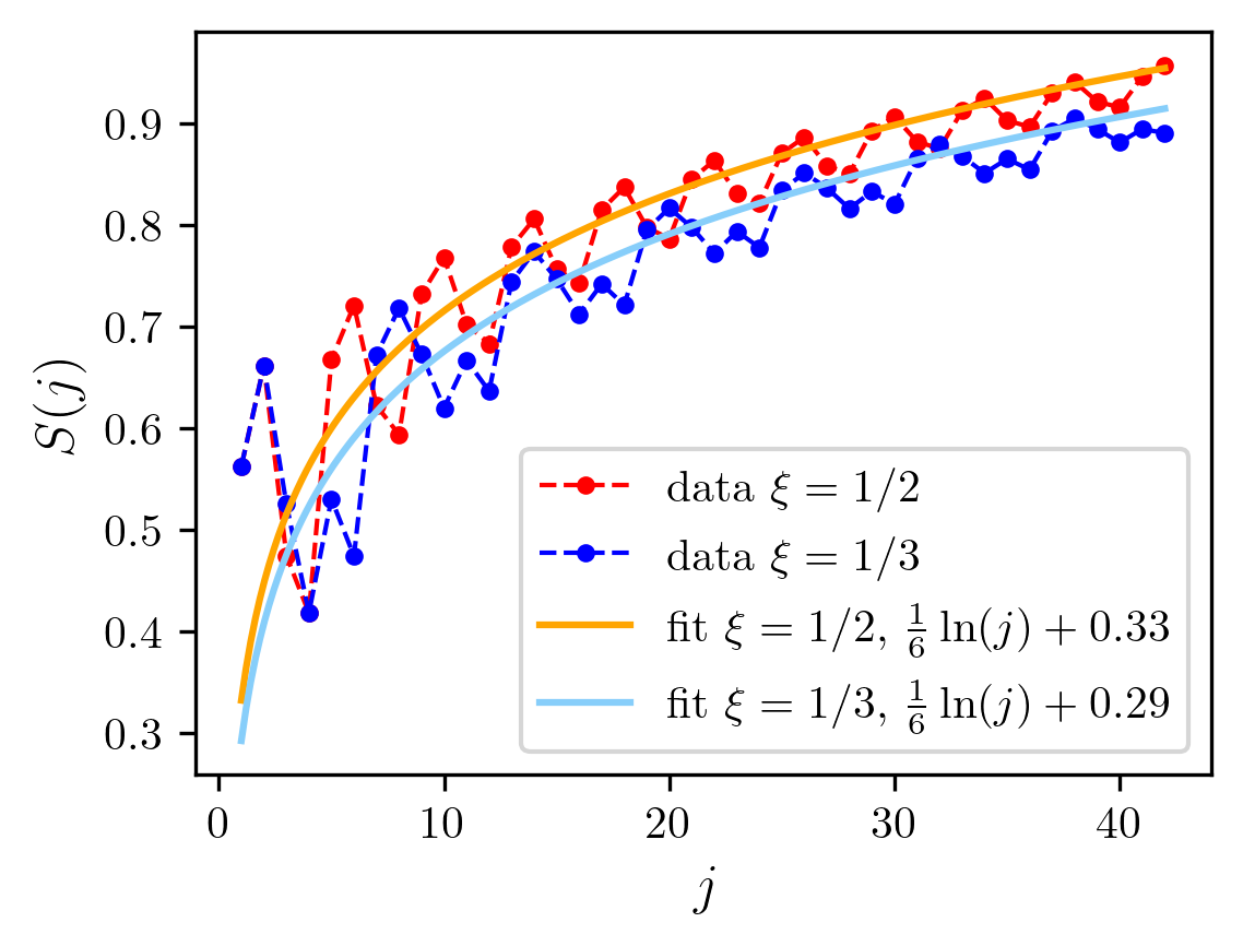
We fix the ratios and and use (53) to compute via exact numerical diagonalization of the chopped correlation matrix (51). Physically, the ratio corresponds to the filling fraction, whereas is (one minus) the aspect ratio, namely the ratio between the size of the chain, and the length of the complement of the intersection between and the chain. We present our numerical results for chains at half-filling, , in Fig. 3. We find a scaling of the form
| (62) |
in the limit of large . This corresponds to a logarithmic violation of the area law in one dimension [6], which is typical for one-dimensional free-fermion models described by an underlying CFT with central charge . The scaling (62) thus suggests that the anti-Krawtchouk chain is described by a CFT in curved space [36] with , similarly to the Krawtchouk chain [32, 34].
The presence of oscillations in Fig. 3 can be attributed to sub-leading terms that have not been fully characterized in the present analysis. Similar oscillations have been observed in Krawtchouk chains and a conjecture regarding the sub-leading terms was proposed in [34].
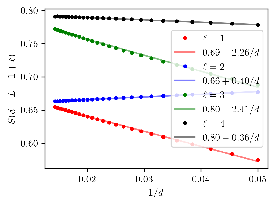
For a fixed filling ratio , a fixed ratio and a fixed subsystem size in the chain, the entanglement entropy rather converges at large diameter to a constant value,
| (63) |
Here, the bound on the entanglement entropy is determined by its value for a maximally entangled state given a subsystem of size . Numerical analysis verifies that the magnitude of remains close to even for , indicating as expected that most of the entanglement originates from a highly entangled state at the boundary, see Fig. 4.
3.5 Large diameter limit of the folded cube
Let us fix the ratio , where is the diameter of the region in the folded cube and is the diameter of the graph. We shall now consider how the entanglement entropy scales in the limit of large diameter at half-filling . From numerical tests and the scaling given by (62) and (63), we find that the behavior of is captured by
| (64) |
In the first situation, , the scaling behavior follows equation (62). For , the contribution arises from anti-Krawtchouk chains that do not intersect with the region , resulting in a zero contribution. In the third regime, , the chains have a small intersection with the region compared to their size of ; the region in these chains is predominantly composed of a highly entangled site on the boundary, leading to a contribution of to .
In the limit of large diameter, Stirling’s formula provides an asymptotic expression for the degeneracy,
| (65) |
In particular, one notes that the degeneracy reaches a peak at and then gets exponentially small as increases. It follows that the largest contribution to the entanglement entropy is coming from terms in equation (52) for which is small but larger than . This corresponds to the third regime and justifies the following expression for the scaling of :
| (66) |
Using the bound (63) on , we find that the entanglement entropy at large and fixed and , is bounded by a strict area law, with no logarithmic enhancement,
| (67) |
Here, we used the following approximation for the area of the boundary ,
| (68) |
which also corresponds to the number of anti-Krawtchouk chains intersecting the region .
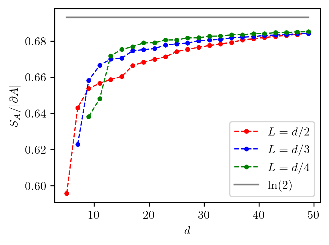
Furthermore, since converges at large to a value near (as shown in Fig. 4), a good estimate of the magnitude of is provided by , as illustrated in Fig. 5.
Equation (67) exhibits a strict area law, which is atypical for critical free-fermion systems that usually display logarithmic enhancements of the area law in the scaling of the entanglement entropy. This behavior aligns with observations made for entanglement entropy in free fermions on high-dimensional structures such as Hamming and Johnson graphs [16, 18, 17].
The underlying cause can be attributed to the high-dimensional geometry of these graphs, wherein the majority of degrees of freedom on the boundary of region do not fully perceive the system’s entire diameter. To be more specific, these graphs can be effectively decomposed into a combination of one-dimensional systems, most of which have only a small fraction of their degrees of freedom originating from the region and its boundary . From the perspective of the free-fermion chains within this decomposition, the process of taking the large-diameter limit of the graph does not correspond to a thermodynamic limit. As a result, their contribution to the entanglement entropy does not give rise to logarithmic enhancements. The area law for entanglement in ground states is a highly local property, caused by correlations of degrees of freedom close to the boundary. Therefore, we expect our findings to hold at leading order for arbitrary regions with volume, not only for the symmetric balls defined in (30). However, our analytical methods are not applicable in such cases, and numerical calculations are cumbersome due to the exponentially large dimension of the Hilbert space.
4 Entanglement Hamiltonian and Heun operator
While the entanglement entropy gives insight into the entanglement properties of the ground state, a more complete picture lays in the reduced density matrix and the entanglement Hamiltonian . Since the ground state is the product of ground states of anti-Krawtchouk chains (57) onto which the projector acts simply, the reduced density matrix can be decomposed as
| (69) |
The entanglement Hamiltonian can further be expressed as a sum of quadratic operators acting on individual chains,
| (70) |
| (71) |
where the matrix is defined in (26).
The characterization of the reduced density matrix thus amounts to describing the entanglement Hamiltonian for each anti-Krawtchouk chain. To streamline the analysis, we will focus on a single chain, denoted as , or a single module at a time and use the following abbreviated notation:
| (72) |
4.1 Commuting Heun operator and
In order to describe , we are interested in the identification of the matrix . It can be done using the correlation matrix as an input in the formula [28]. This is straightforward but does not provide an explicit formula for the entries . Moreover, it can be numerically unstable due to the proximity of most eigenvalues of to and . An alternative method is to use the fact that admits a simple commuting operator known as a generalized algebraic Heun operator ,
| (73) |
where the coefficients and are given by
| (74) |
Indeed, one can check using the representation of and in the basis of vectors that . Similarly, the basis of vectors makes it straightforward to check that the Heun operator commutes with the projector onto region , i.e. . It then follows that,
| (75) |
A commuting Heun operator also exists for homogeneous free fermion chains and a wide range of inhomegenous models [23, 24, 25, 37, 38, 33, 39, 34, 35]. Understanding precisely the relation between these commuting tridiagonal matrices, correlation matrices and entanglement Hamiltonians has attracted some attention (notably in the homogeneous case [23, 24, 25, 38]) but remains in general an open question. Our aim is to express as a sum of powers of . More precisely, we are interested in the possibility of approximating as an affine transformation of the Heun operator. The matrix is irreducible tridiagonal in the basis and is thus non-degenerate on . It further commutes with so they can be related on this subspace by the following sum,
| (76) |
where is the dimension of the subspace and the coefficients are fixed such that both sides of equation (76) have the same set of eigenvalues. Since we are examining the ground state of a local system, we anticipate that the dominant elements of correspond to the hopping terms between neighboring sites. Given that the Heun operator exclusively connects nearest neighbors, i.e.
| (77) |
it suggests that could be approximated to some extent by the first two powers of ,
| (78) |
where and are left to be determined. For example, this relation with and holds in the continuum limit of homegeneous one-dimensional chains at half filling [38], where is the length of the interval. For general and , one can define an Hamiltonian and density matrix as
| (79) |
and
| (80) |
A natural idea to determine the coefficients is to minimize the distance between and the expansion (76). However, this method is not efficient when the number of parameters is greater than one [40]. Our approach to fix the parameters and is to require that and agree on the expectation value of observables. Specifically, these density matrices can be selected such that they coincide in the expected number of particles and the von Neumann entropy in the anti-Krawtchouk chain ,:
| (81a) | |||
| (81b) |
where is the operator counting the number of particles in the intersection of the region with the chain ,
| (82) |
4.2 Rényi fidelities and Réyni entropies of and
In this section we compare the reduced density matrix with the affine approximation , where and are fixed by the constraints (81). To achieve this, we compute their Rényi fidelities and their respective Rényi entropies.
Quantum fidelities quantify the resemblance between two quantum states [41, 42]. Importantly, fidelities can be used to detect and characterize quantum phase transitions [43, 44, 45, 46, 47, 48, 49, 50, 51], similarly to the entanglement entropy. Rényi fidelities [26] were introduced recently as a generalization of Uhlmann-Jozsa fidelity [41, 42]. They are defined for general density matrices and as
| (83) |
and they verify the following properties,
| (84a) | |||
| (84b) |
In the case of Gaussian fermionic states, the formula (83) for Réyni fidelities reduces to an expression in terms of the eigenvalues of the correlation matrices of and [26]. Applying this result to the commuting states and , one finds
| (85) |
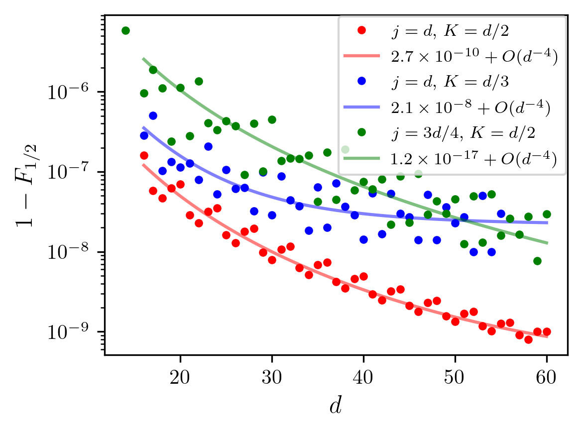
The results of numerical computation of (85) for and diameters of up to are shown in Fig. 6. In particular, seems to converge to a value very close to in the large-diameter limit. A similar behavior was also observed for general values of . The high fidelities between the two states demonstrate that captures the essence the reduced density matrix , confirming the validity of the linear approximation (78) and the local nature of the state . It also suggests that density matrices based on an affine transformation of Heun operators could offer a convenient approximation of the reduced density matrix of free-fermion ground states in other settings.
The proximity of the states and is further visible in their respective Réyni entropies. Indeed, one can consider their deviation defined as
| (86) |
where are the Rényi entropies,
| (87) |
Let us note that it is distinct from the relative entropy between and , which also measures the proximity between two quantum states [52] and would deserve an investigation of its own in this setting.
Using the known relation between and the matrix [53], can be expressed as
| (88) |


Numerically, we find that the deviation is small relative to for all when fixing and such that the constraints (81) are verified, see Fig. 7. Imposing that the two states have the same average number of particles and von Neumann entropy is thus sufficient to ensure that and share a similar entanglement spectrum.
5 Conclusion
The scaling behavior of the ground-state entanglement entropy was investigated for a model of free fermions defined on the vertices of a folded cube. In the limit of large diameter, the entanglement entropy was found to obey a strict area law without any logarithmic enhancement. This departure from the behavior observed in free-fermion systems on cubic lattices can be attributed to the intricate geometric structure of folded cubes. Specifically, these structures can be effectively decomposed into a collection of chains, most of which only have a small intersection with the subsystem compared to the graph’s diameter. From the perspective of these chains, the thermodynamic limit of folded cubes with and a fixed aspect ratio maps to a thermodynamic limit of one-dimensional systems having aspect ratios approaching zero, and hence giving no logarithmic enhancement.
A similar phenomenon and explanation should hold for the thermodynamic limits of free fermions on sequences of other distance-regular graphs with increasing diameter. It would be intriguing to investigate whether the rich symmetries of distance-regular graphs are essential or if similar patterns emerge in a wide range of high-dimensional graphs.
Additionally, we explored the relationship between the entanglement Hamiltonian and the Heun operator. It was observed that the reduced density matrix and a Gaussian state of a Hamiltonian constructed through an affine transformation of the Heun operator have Réyni fidelities close to one, provided that both matrices possess equal expectations of particle number and von Neumann entropy. It was also shown that they have similar Réyni entropies. It suggests that free-fermion Hamiltonians based on generalized Heun operators offer adequate approximation of entanglement Hamiltonians. Future investigations could look into alternative constraints on the affine transformation so as to possibly find higher fidelities, a more accurate alignment of the Rényi entropies and, consequently, a better approximation of the entanglement Hamiltonian.
Acknowledgement
We thank Riccarda Bonsignori for useful discussion and correspondence. ZM was supported by USRA scholarships from NSERC and FRQNT. PAB holds an Alexander-Graham-Bell scholarship from the Natural Sciences and Engineering Research Council of Canada (NSERC). GP holds a FRQNT and a CRM–ISM postdoctoral fellowship, and acknowledges support from the Mathematical Physics Laboratory of the CRM. The research of LV is funded in part by a Discovery Grant from NSERC.
References
- [1] L. Amico, R. Fazio, A. Osterloh, and V. Vedral, “Entanglement in many-body systems,” Rev. Mod. Phys. 80, 517 (2008).
- [2] N. Laflorencie, “Quantum entanglement in condensed matter systems,” Phys. Rep. 646, 1 (2016).
- [3] A. Osterloh, L. Amico, G. Falci, and R. Fazio, “Scaling of entanglement close to a quantum phase transitions,” Nature 416, 608 (2002).
- [4] T. J. Osborne and M. A. Nielsen, “Entanglement in a simple quantum phase transition,” Phys. Rev. A 66, 032110 (2002).
- [5] G. Vidal, J. I. Latorre, E. Rico, and A. Kitaev, “Entanglement in quantum critical phenomena,” Phys. Rev. Lett. 90, 227902 (2003).
- [6] P. Calabrese and J. L. Cardy, “Entanglement entropy and quantum field theory,” J. Stat. Mech. P06002 (2004).
- [7] P. Calabrese and J. L. Cardy, “Entanglement entropy and conformal field theory,” J. Phys. A: Math. Theor. 42, 504005 (2009).
- [8] A. Kitaev and J. Preskill, “Topological entanglement entropy,” Phys. Rev. Lett. 96, 110404 (2006).
- [9] M. Levin and X.-G. Wen, “Detecting topological order in a ground state wave function,” Phys. Rev. Lett. 96, 110405 (2006).
- [10] P. Calabrese and J. L. Cardy, “Evolution of entanglement entropy in one-dimensional systems,” J. Stat. Mech. P04010 (2005).
- [11] M. Fagotti and P. Calabrese, “Evolution of entanglement entropy following a quantum quench: Analytic results for the XY chain in a transverse magnetic field,” Phys. Rev. A 78, 010306 (2008).
- [12] C. Gogolin and J. Eisert, “Equilibration, thermalisation, and the emergence of statistical mechanics in closed quantum systems,” Rep. Prog. Phys. 79, 056001 (2016).
- [13] V. Alba and P. Calabrese, “Entanglement and thermodynamics after a quantum quench in integrable systems,” Proceedings of the National Academy of Sciences 114, 7947 (2017).
- [14] D. Gioev and I. Klich, “Entanglement entropy of fermions in any dimension and the Widom conjecture,” Phys. Rev. Lett. 96, 100503 (2006).
- [15] W. Li, L. Ding, R. Yu, T. Roscilde, and S. Haas, “Scaling behavior of entanglement in two- and three-dimensional free-fermion systems,” Phys. Rev. B 74, 073103 (2006).
- [16] P.-A. Bernard, N. Crampé, and L. Vinet, “Entanglement of free fermions on Hamming graphs,” Nucl. Phys. B 986, 116061 (2023).
- [17] G. Parez, P.-A. Bernard, N. Crampé, and L. Vinet, “Multipartite information of free fermions on Hamming graphs,” Nucl. Phys. B 990, 116157 (2023).
- [18] P.-A. Bernard, N. Crampé, and L. Vinet, “Entanglement of free fermions on Johnson graphs,” J. Math. Phys. 64, 061903 (2023).
- [19] G. M. Brown, “Hypercubes, Leonard triples and the anticommutator spin algebra,” arXiv:1301.0652 [math.CO].
- [20] P. Terwilliger, “The subconstituent algebra of an association scheme (Part I),” J. Algebr. Comb. 1, 363 (1992).
- [21] P. Terwilliger, “The subconstituent algebra of an association scheme (Part II),” J. Algebr. Comb. 2, 73 (1993).
- [22] P. Terwilliger, “The subconstituent algebra of an association scheme (Part III),” J. Algebr. Comb. 2, 177 (1993).
- [23] V. Eisler and I. Peschel, “Free-fermion entanglement and spheroidal functions,” J. Stat. Mech P04028 (2013).
- [24] V. Eisler and I. Peschel, “Analytical results for the entanglement Hamiltonian of a free-fermion chain,” J. Phys. A: Math. Theor. 50, 284003 (2017).
- [25] V. Eisler and I. Peschel, “Properties of the entanglement Hamiltonian for finite free-fermion chains,” J. Stat. Mech. 104001 (2018).
- [26] G. Parez, “Symmetry-resolved Rényi fidelities and quantum phase transitions,” Phys. Rev. B 106, 235101 (2022).
- [27] A. E. Brouwer, W. H. Haemers, A. E. Brouwer, and W. H. Haemers, Distance-regular graphs. Springer, 2012.
- [28] I. Peschel, “Calculation of reduced density matrices from correlation functions,” J. Phys. A: Math. Gen. 36, L205 (2003).
- [29] V. X. Genest, L. Vinet, G.-F. Yu, and A. Zhedanov, Supersymmetry of the Quantum Rotor, in Frontiers in Orthogonal Polynomials and -Series, ch. 15, pp. 291–305. World Scientific, (2018).
- [30] N. Crampé, R. I. Nepomechie, and L. Vinet, “Free-Fermion entanglement and orthogonal polynomials,” J. Stat. Mech. 093101 (2019).
- [31] F. Finkel and A. González-López, “Inhomogeneous XX spin chains and quasi-exactly solvable models,” J. Stat. Mech. 093105 (2020).
- [32] F. Finkel and A. González-López, “Entanglement entropy of inhomogeneous XX spin chains with algebraic interactions,” JHEP 1 (2021).
- [33] N. Crampé, R. I. Nepomechie, and L. Vinet, “Entanglement in fermionic chains and bispectrality,” Rev. Math. Phys. 33, 2140001 (2021).
- [34] P.-A. Bernard, N. Crampé, R. I. Nepomechie, G. Parez, L. P. d’Andecy, and L. Vinet, “Entanglement of inhomogeneous free fermions on hyperplane lattices,” Nucl. Phys. B 984, 115975 (2022).
- [35] P.-A. Bernard, G. Carcone, N. Crampe, and L. Vinet, “Computation of entanglement entropy in inhomogeneous free fermions chains by algebraic Bethe ansatz,” arXiv:2212.09805 [math-ph].
- [36] J. Dubail, J.-M. Stéphan, J. Viti, and P. Calabrese, “Conformal field theory for inhomogeneous one-dimensional quantum systems: the example of non-interacting Fermi gases,” SciPost Phys. 2, 002 (2017).
- [37] F. A. Grünbaum, L. Vinet, and A. Zhedanov, “Algebraic Heun operator and band-time limiting,” Commun. Math. Phys. 364, 1041 (2018).
- [38] V. Eisler, E. Tonni, and I. Peschel, “On the continuum limit of the entanglement Hamiltonian,” J. Stat. Mech 073101 (2019).
- [39] P.-A. Bernard, N. Crampé, D. Shaaban Kabakibo, and L. Vinet, “Heun operator of lie type and the modified algebraic Bethe ansatz,” J. Math. Phys. 62, 083501 (2021).
- [40] R. Bonsignori and V. Eisler, “Private communication,” (2023).
- [41] A. Uhlmann, “The ‘transition probability’ in the state space of a -algebra,” Rep. Math. Phys. 9, 273 (1976).
- [42] R. Jozsa, “Fidelity for Mixed Quantum States,” J. Mod. Opt. 41, 2315 (1994).
- [43] H. T. Quan, Z. Song, X. F. Liu, P. Zanardi, and C. P. Sun, “Decay of Loschmidt Echo Enhanced by Quantum Criticality,” Phys. Rev. Lett. 96, 140604 (2006).
- [44] H.-Q. Zhou and J. P. Barjaktarevič, “Fidelity and quantum phase transitions,” J. Phys. A: Math. Theor. 41, 412001 (2008).
- [45] S.-J. Gu, “Fidelity approach to quantum phase transitions,” Int. J. Mod. Phys. B 24, 4371 (2010).
- [46] J. Dubail and J.-M. Stéphan, “Universal behavior of a bipartite fidelity at quantum criticality,” J. Stat. Mech. L03002 (2011).
- [47] J.-M. Stéphan and J. Dubail, “Logarithmic corrections to the free energy from sharp corners with angle ,” J. Stat. Mech. P09002 (2013).
- [48] C. Hagendorf and J. Liénardy, “Open spin chains with dynamic lattice supersymmetry,” J. Phys. A: Math. Theor. 50, 185202 (2017).
- [49] G. Parez, A. Morin-Duchesne, and P. Ruelle, “Bipartite fidelity of critical dense polymers,” J. Stat. Mech. 103101 (2019).
- [50] A. Morin-Duchesne, G. Parez, and J. Liénardy, “Bipartite fidelity for models with periodic boundary conditions,” J. Stat. Mech. 023101 (2021).
- [51] C. Hagendorf and G. Parez, “On the logarithmic bipartite fidelity of the open XXZ spin chain at ,” SciPost Phys. 12, 199 (2022).
- [52] M. A. Nielsen and I. L. Chuang, Quantum Computation and Quantum Information: 10th Anniversary Edition. Cambridge University Press, 2010.
- [53] J. A. Carrasco, F. Finkel, A. Gonzalez-Lopez, and P. Tempesta, “A duality principle for the multi-block entanglement entropy of free fermion systems,” Sci. Rep. 7, 11206 (2017).
Appendix A Anti-Krawtchouk polynomials
The monic anti-Krawtchouk polynomials satisfy the following three-term recurrence relation,
| (89) |
where
| (90) |
The polynomials are given in terms of generalized hypergeometric series as
| (91) |
where is a coefficient given by
| (92) |
and is the Pochhammer symbol.
The monic anti-Krawtchouk polynomials are orthogonal on the grid
| (93) |
with the weight function
| (94) |
Indeed, their non-monic counterpart defined by
| (95) |
verify the following two orthogonality relations,
| (96) |
where is a normalisation factor given by
| (97) |
They further solve the recurrence relation (49),
| (98) |
where
| (99) |
Since the bases and of are respectively orthonormal, the overlaps are given by
| (100) |