Unified Modeling and Rate Coverage Analysis for Satellite-Terrestrial Integrated Networks:
Coverage Extension or Data Offloading?
Abstract
With the growing interest in satellite networks, satellite-terrestrial integrated networks (STINs) have gained significant attention because of their potential benefits. However, due to the lack of a tractable network model for the STIN architecture, analytical studies allowing one to investigate the performance of such networks are not yet available. In this work, we propose a unified network model that jointly captures satellite and terrestrial networks into one analytical framework. Our key idea is based on Poisson point processes distributed on concentric spheres, assigning a random height to each point as a mark. This allows one to consider each point as a source of desired signal or a source of interference while ensuring visibility to the typical user. Thanks to this model, we derive the probability of coverage of STINs as a function of major system parameters, chiefly path-loss exponent, satellites and terrestrial base stations’ height distributions and density, transmit power and biasing factors. Leveraging the analysis, we concretely explore two benefits that STINs provide: i) coverage extension in remote rural areas and ii) data offloading in dense urban areas.
Index Terms:
Satellite-terrestrial integrated network, stochastic geometry, rate coverage probability.I Introduction
Recent advances in low Earth orbit (LEO) satellite technologies are recognized as a breakthrough not only in the space industry, but also in wireless communications. With the decreasing cost of launching LEO satellites, tens of thousands of LEO satellites are planned to be deployed (e.g., SpaceX Starlink [1]), which enables the structuration of ultra-dense wireless networks above the Earth. One promising way to leverage satellite networks is to integrate them with the existing terrestrial network, creating a mutually complementary system that operates seamlessly [2, 3, 4]. This motivates the advent of satellite-terrestrial integrated networks (STINs). In the literature, two main benefits of STINs have mainly been discussed:
- •
- •
Notwithstanding these potential advantages, there has been a dearth of analytical studies investigating the rate coverage performance of STINs. A main hindrance is the lack of a unified network model that jointly captures satellite and terrestrial networks simultaneously. In this work, we address this challenge by proposing such a unified model. Leveraging this model, we analyze the rate coverage performance of STINs, which allows one to foresee the benefits of these new architectures.
I-A Related Work
The use of stochastic geometry has played a crucial role in modeling and analyzing wireless networks [8, 9]. In particular, much of the prior work has focused on the investigation of terrestrial cellular networks. This analysis involves the distribution of a random point process on the 2D plane to model the spatial locations of the BSs. With this methodology, a wide range of cellular network types, including HetNets [10, 11], multi-antenna cellular networks [12, 13], millimeter wave (mmWave) cellular networks [14, 15], and UAVs networks [16, 17] were actively explored.
Recently, with the growing interest in satellite communication systems, satellite network analysis based on tools of stochastic geometry gained great momentum [18, 19, 20, 21, 22, 23, 24]. For instance, in [20], the coverage probability of satellite networks was derived by modeling the satellite locations as a binomial point process (BPP) distributed on a certain sphere. This work was improved in [21] by incorporating a non-homogeneous distribution of satellites. In [22], the technique of [20] was employed with different fading scenarios. Despite the popularity of the BPP based analysis, this model inevitably entails complicated expressions, which limits tractability. Addressing this, in [24], an analytical approach exploiting conditional Poisson point process (PPP) was proposed, wherein the PPP was distributed on a certain sphere. The coverage analysis was then conducted by conditioning on the fact that at least one satellite is visible to the typical user. This makes the analytical expressions much more tractable than those of the BPP. Additionally, it was also shown that the analysis of [24] reflects well the actual coverage trend drawn by using realistic Starlink constellation sets.
Compared to the analysis of terrestrial networks, one crucial difference in the modeling of satellite networks is the use of a spherical point process, wherein a random point process (either PPP or BPP) is distributed on a certain sphere to model the satellite locations. The disparity between the modeling methodology used for the satellite and terrestrial networks (i.e., a planar point process vs. a spherical point process) is the main challenge to unify them into a single model for analyzing the STIN. Recently, cooperative space, aerial, and terrestrial networks have been actively studied in [25, 26, 27, 28, 29]. Nonetheless, the network models presented in the these references are limited to providing a comprehensive understanding of STINs yet. For example, [26] considered a spherical point process for modeling satellite networks and a planar point process for modeling terrestrial networks separately. This separated approach cannot capture the full geometries of STINs. In [25], a single satellite was considered, which is not adequate when dealing with dense satellite networks. In [27], a single geostationary (GEO) satellite and multiple aircrafts with different altitudes were considered, in which the locations of aircrafts were modeled by using a two dimensional (2D) Poisson Line Process (PLP). This model is useful to study cooperation between a single satellite and a number of aircrafts by incorporating safety distances between aircrafts; yet it cannot be used to represent a large scale STIN where spatial locations of satellites and terrestrial BSs are modeled on spheres. Consequently, there is a gap in the literature regarding the rate coverage analysis of STINs with a unified network modeling, and filling up this gap is the primary motivation of our work.
I-B Contributions
In this paper, we consider the downlink of a STIN, in which a user can be served either from a satellite or a terrestrial BS sharing the same spectrum (i.e., the scenario is referred as an open network). The user selects its association based on the averaged reference signal power including bias factors, where the latter can be used to control the load as in heterogeneous networks (HetNets) [10, 11]. Further, the user experiences the interference coming from both the satellites and the terrestrial BSs. In this setup, our aim is to model and analyze the rate coverage performance of the considered STIN, and to provide STIN system design insights leveraging the analysis. We summarize our contributions as follows.
-
•
Unified modeling: For modeling the STIN, it is of central importance to jointly capture the key characteristics of the satellite and the terrestrial networks. Since this is not feasible with the existing network models, we propose a novel network model. In our model, a homogeneous PPP is first distributed on two concentric spheres, where the inner sphere represents the Earth and the outer sphere represents the satellite orbital sphere. Then, a random height is assigned to each point, so that each satellite and terrestrial BS has a different altitude. This is a key distinguished feature compared to the previous models [24, 20, 18, 19] where all points are at the same altitude. The random height feature has two important motivations. First, this makes our model more realistic, as it can reflect a realistic satellite network where satellites have different altitudes [1]. Second, the random height is a key to unify the satellite and the terrestrial networks into a single analytical framework. Without positive random height, the terrestrial network cannot be modeled by using a spherical point process distributed on the Earth since there is no mathematical visibility between a user and any other terrestrial BS. We will explain this in more detail in Remark 1.
-
•
Rate coverage analysis: Based on the proposed model, we derive an expression for the coverage probability as a function of the system parameters, chiefly the densities, path-loss exponents, height geometries (maximum/minimum altitudes and height distributions), and bias factors of the satellites and the terrestrial BSs. To this end, we first obtain the visibility probability of the satellite and the terrestrial networks, that characterizes the probability that a user sees at least one satellite/terrestrial BS that it can communicate with. We note that this is not straightforward from the existing result [24] since each satellite/terrestrial BS has a random altitude in our model. Using this, we compute the conditional nearest satellite/terrestrial BS distance distribution and also the probability that a user is associated with the satellite/terrestrial network. Leveraging these, we derive the rate coverage probability of the STIN under the assumption of Shadowed-Rician fading for the satellite links and Nakagami- fading for the terrestrial links.
-
•
Analysis of STIN benefits and design insights: Using our analysis, we concretely explore the two benefits of the STIN architecture: coverage extension in remote rural areas and data offloading in dense urban areas. This leads to some valuable system design insights: 1) In remote rural areas where the terrestrial BSs’ deployment density is very low, the STIN offers huge coverage enhancement. However, due to satellite interference, it is crucial to control the satellite density properly. 2) In dense urban areas where the user density is high, in the STIN, data traffic can be pushed to the satellite from the terrestrial BSs, provided that the satellite density, the beamforming gains, and the bias are suitably selected.
II System Model
II-A Network Model
Poisson point process on a sphere: To model the spatial locations of satellite and terrestrial BS, we consider PPPs distributed on a sphere (SPPP) [24]. For better understanding, we first introduce a generic SPPP model with random heights, and then present the specific model for the satellite and terrestrial networks, respectively.
Consider a sphere defined in whose center is the origin and radius is fixed as . This sphere is denoted as . Let be an isotropic PPP on . We denote the point of this point process as and denote the density of as . The number of points on the sphere is a random variable drawn from the Poisson distribution with mean . Conditional on the fact that there are points, these points are independently and uniformly distributed on . The number of points of located in a particular set is denoted as .
As the deployment density of the satellite network increases, the analytical coverage probability derived under a homogeneous SPPP model and the actual coverage probability computed by using a realistic Starlink constellation set closely match as demonstrated in [24]. This justifies the use of a homogeneous SPPP to model dense satellite networks.
Random heights: Based on the PPP , we construct a new point process by displacing each point of from the sphere by a certain height. Denoting by the height of point , we define the new point as , so that . The heights of the points are assumed to be independent and identically distributed (IID) random variables drawn from a certain distribution on . Correspondingly, we let be the cumulative distribution function (CDF) of the heights. The points of this point process are hence . Note that can be seen as a marked PPP generated from , wherein the mark of the point at is the height . Throughout the paper, we assume a positive height, , .
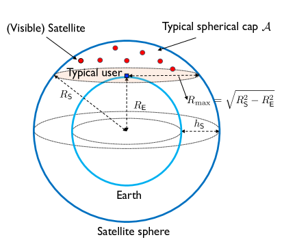
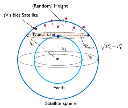
Satellite network: We now describe the satellite network model. Consider two spheres sharing the same origin. We define the radii of these spheres as and , respectively. The sphere with radius represents the Earth and the sphere with radius represents the satellite orbital sphere. We also define , where is the standard satellite altitude. We now distribute a SPPP on , denoted as with density . Upon this, we displace point from the satellite orbital sphere by a random height , which builds . The support of will be denoted as . In this modeling, represents a snapshot of the satellite spatial locations. If for all , then each satellite is located at the same altitude of , which corresponds to the network model in [24].
For ease of understanding, we depict the conventional satellite network model without random heights and the considered satellite network model with random heights in Fig 1.
Terrestrial network: Similar to the satellite network, we consider a SPPP with random heights to model the terrestrial network. We first distribute a SPPP with the density on the sphere with radius and denote this point process as . Subsequently, incorporating random heights into , we have . A snapshot of the spatial locations of terrestrial BSs is modeled by . The support of is denoted by . If for all , all terrestrial BSs are located on the surface of the Earth. We also assume .
Typical user: We also model the users’ locations as a homogeneous SPPP with density . Per Slivnyak’s theorem [8], we focus on the typical user located on in Cartesian coordinates. We point out that this does not affect the statistical distribution of and .

Typical spherical cap: Since the satellites and the terrestrial BSs are distributed on certain spheres, some points are not visible from the typical user. If so, they are neither counted as a potential source of desired signal nor as contributing to the interference. For this reason, characterizing the visibility is crucial in the coverage analysis. To this end, we use the concept of typical spherical cap.
At first, we focus on the terrestrial network. Consider a point is on sphere and its image point with height , so that is on sphere . Recalling that the typical user is located at , the outer typical spherical cap of radius , , is defined as the set of points in whose distance to the typical user is no larger than :
| (1) |
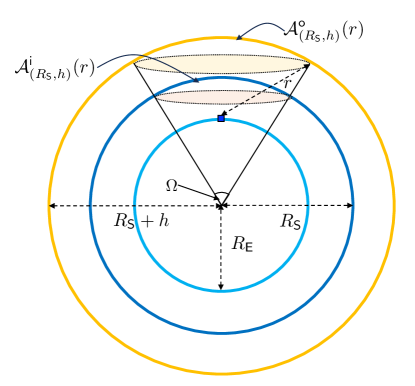
We provide an illustration for in Fig. 2-(a). It is worth to mention that given , we will focus on , with
| (2) |
If , then is the portion of sphere cut off by the plane tangent to the sphere (the Earth) at . The inner typical spherical cap is the spherical cap of that has the same solid angle as , namely,
| (3) |
We also provide an illustration of the inner typical spherical cap in Fig. 2-(a). In Fig. 2, we observe that, seen from the origin, the solid angles of and are the same. The inner typical spherical cap is the region of the points which are mapped to the points .
Now we investigate the areas of the typical spherical caps. In the terrestrial network, the area of the outer typical spherical cap is obtained as
| (4) |
where
| (5) |
by using Archimedes’ Hat-Box Theorem [30]. By the definition of the solid angle, we have
| (6) |
Then the area of the inner typical spherical cap is given by
| (7) |
When , the area of the outer/inner typical spherical caps are simplified to
| (8) |
When , the areas of the outer/inner typical spherical caps are .
Next, similar to the terrestrial network case, we define the outer and the inner typical spherical caps corresponding to the satellite network as and by following (1) and (3). Specifically, we have
| (9) |
where with
| (10) |
The area of the outer typical spherical cap is calculated as
| (11) |
Accordingly, when , then
| (12) |
The inner typical spherical cap is defined as
| (13) |
where its area is
| (14) |
When , the areas of the outer/inner typical spherical caps are . We depict the outer/inner typical spherical caps of the satellite network in Fig. 2-(b).
With the defined typical spherical caps, we are able to identify the visibility of the terrestrial BSs or the satellites. For example, in the terrestrial network, the terrestrial BS with height (located at ) is visible to the typical user if and only if (or equivalently, ). This is because, if , then is located below the horizon, and the visibility is blocked by the Earth. The satellite visibility is also identified in an equivalent manner.
To characterize the visibility, we assume a set of terrestrial BSs whose heights are in and denote such a point process as and . The event that the typical user can observe at least one terrestrial BS is equivalent with the event that any of includes at least one visible terrestrial BS, namely,
| (15) |
Similar to this, denoting a point process of the satellites with heights included in as and , the event that the typical user can observe at least one satellite is
| (16) |
For simplicity, we denote the average number of visible satellites and of visible terrestrial BSs as and , respectively.
One key difference of the visibility in the proposed network model and the conventional network model [24] is that, in the proposed network model, the visibility is jointly determined not only by the points’ spatial locations, but also their heights. Namely, even if two satellites are located at the same position in , it is possible that one satellite is visible and the other one is not because of their different altitudes. In general, the higher the altitude, the more likely the visibility of the point from the typical user. This is the main reason to define multiple typical spherical caps depending on .
II-B Channel Model
The path-loss between the satellite located at and the typical user located at is defined as , where is the path-loss exponent for the satellite network. Likewise, the path-loss between the terrestrial BS located at and the typical user is defined as , where is the path-loss exponent for the terrestrial network. The wireless propagation environments of the satellite network and the terrestrial network are reflected into and . For instance, if the propagation between a satellite and a user is line-of-sight (LoS), then . If we consider an urban communication scenario with rich scattering for the terrestrial network, .
As the small-scale fading, we use the Shadowed-Rician channel model for the satellite links and the Nakagami- channel model for the terrestrial links. We first explain the Shadowed-Rician model, then characterize the Nagakami- model. The Shadowed-Rician channel model is known to accurately characterize the compound effects on the satellite channels’ medium and small-scale fading effects [31]. The probability density function (PDF) of the Shadowed-Rician fading envelope is presented as
| (17) |
where is the fading envelope corresponding to the satellite , is the confluent hypergeometric function of the first kind, and are the average power of the scatter component and LoS component respectively, and is the Nakagami parameter (for satellite communications). We denote and . For integer , the confluent hypergeometric function is computed as
| (18) |
where is the Pochhammer symbol defined as . Using (18), we obtain the PDF of the Shadowed-Rician fading power as
| (19) |
Now we explain the Nakagami- channel model. In this model, , which is the fading envelope corresponding to the terrestrial BS , is distributed according to the probability density function (PDF) given by:
| (20) |
where is the Gamma function and is the Nakagami parameter for terrestrial communications. Note that we use to differentiate it from the satellite Nakagami parameter defined as . With , the fading scenario is reduced to the Rayleigh fading. The PDF of the Nakagami- fading power is obtained as
| (21) |
We now explain the directional beamforming gain model. We adopt the sectored antenna model, wherein the directional beamforming gains are approximated as a rectangular function [32, 14]. In such an approximation, a user gets the main-lobe gain when it is included within the main-lobe, otherwise the user has the side-lobe gain. The sectored antenna model has been widely used in stochastic geometry based analysis because it is not only analytically tractable, but it is also suitable to reflect the primary features of the directional beamforming. In this model, the beamforming gains in the satellite network are expressed as
| (22) |
where (or ) is the main-lobe (or the side-lobe) beamforming gains offered at a satellite, and (or ) is the main-lobe (or the side-lobe) beamforming gains obtained at a user. We assume that only the associated satellite has and the other interfering satellites have . The beamforming gains in the terrestrial network are defined in the similar manner.
II-C Cell Association
To control the user populations connected to each network, we apply the biasing factors in association process. When the satellites and the terrestrial BSs use different transmit power ( and ) and biasing factors ( and ), each satellite and terrestrial BS sends reference signals by encompassing the biasing factors, so that the effective transmit power of the reference signal is or . Averaging the randomness regarding the small-scale fading, the typical user is associated with a cell (either in the satellite or the terrestrial networks) whose average received power is strongest. Namely, the associated network and the associated cell index are determined by
| (23) |
Note that our cell association process (23) is equivalent to the method commonly employed for -tier HetNets [10, 11]. Throughout the paper, we use to indicate the network type that the typical user is associated with and assume without loss of generality.
II-D Performance Metric
We separately consider the association cases: 1) association with the satellite network (), 2) association with the terrestrial network (). At first, under the assumption that the typical user is associated with the satellite network, the conditional SINR is defined as
| (24) |
In (24), is the noise power and , where () is the set of interfering satellites (terrestrial BSs) conditioned on that the typical user is connected to the satellite network. Based on (24), letting be the operating bandwidth, the conditional achievable rate is given as . In the same manner, when the typical user is associated with the terrestrial network, the conditional SINR is given as
| (25) |
where . In turn, with the conditional achievable rate , the rate coverage probability is defined as
| (26) | |||
| (27) |
where indicates the probability that the typical user is associated with the network type conditioned on that at least point is visible in the network type , . Further, the visibility probabilities are
| (28) | |||
| (29) |
Remark 1.
[Rationale on random heights] Our model stands out because of its feature of assigning a random height to each point on the two spheres. This feature has two crucial implications. At first, our model is capable of reflecting more realistic scenarios. For instance, the existing network models for the satellite network [20, 21, 24] assumes that every satellite has the same altitude. This model, however, does not properly reflect the reality of satellite networks, as there are variations in the altitudes of individual satellites [1]. Further, in the terrestrial network, terrestrial BSs are installed on a structure such as rooftop or tower with different heights to ensure a wider coverage range. Our model is able to reflect these realistic situations.
Second, the random height is a key to unify the satellite network and the terrestrial network. As mentioned above, the satellite network has been modeled by using a spherical point process model [20, 21, 24], while planar point processes were mainly used for modeling terrestrial networks [33, 12, 15]. To analyze STINs, it is of importance to combine these two disparate networks into one unified model. Although it may be tempting to adopt a spherical point process for both the satellite and terrestrial networks, this is infeasible. This is mainly because, when distributing points on the Earth to model spatial locations of terrestrial BSs, no terrestrial BS is mathematically visible from the typical user since no two points on a sphere can be connected via a straight line that does not intersect the sphere. By assigning random heights on points for terrestrial BSs, we ensure visibility, which makes it feasible to model the terrestrial network with a spherical point process. By doing this, we are able to capture the full complexity of the STIN into one unified analytical framework.
III Mathematical Preliminaries
In this section, before delving into the rate coverage analysis, we present some necessary mathematical ingredients in this section. We start with the probability that at least one satellite is visible from the typical user.
Lemma 1 (Visibility probability of the satellite network).
The number of visible satellites follows the Poisson distribution with parameter . Hence, the probability that at least satellite is visible at the typical user is
| (30) |
Proof.
See Appendix A. ∎
Corollary 1 (Visibility probability of the terrestrial network).
The number of visible terrestrial BS follows the Poisson distribution with parameter . Hence, the probability that at least one terrestrial BS is visible at the typical user is
| (31) |
Proof.
The proof is omitted since it is straightforward from Lemma 1. ∎
Now we derive the distribution of the nearest satellite distance conditioned on that at least satellite is visible as follows.
Lemma 2 (Conditional nearest satellite distance distribution).
Assume that the support of of the satellite networks is . Defining the distance of the nearest satellite to the typical user as , the PDF of conditioned on the fact that at least satellite is visible is
| (32) |
for and 0 otherwise, where
| (33) |
and
| (34) |
and also
| (35) | |||
| (36) |
Proof.
See Appendix B. ∎
Assuming (i.e., all satellites are on a given orbit with height ), the conditional PDF (32) boils down to
| (37) |
for . We observe that (37) is a truncated Rayleigh distribution as shown in [24]. In this sense, Lemma 2 generalizes the prior result in [24].
Similar to the satellite network, we also derive the conditional distribution of the nearest terrestrial BS distance as follows.
Corollary 2 (Conditional nearest terrestrial BS distance distribution).
Assume the support of for the terrestrial networks of the form . Defining the distance of the nearest terrestrial BS to the typical user as , the PDF of conditioned on the fact that at least terrestrial BS is visible is
| (38) |
for and 0 otherwise, where
| (39) |
and
| (40) |
and also
| (41) | |||
| (42) |
Proof.
The proof is omitted since it is straightforward from Lemma 2. ∎
Next, using the acquired conditional nearest distance probabilities, we obtain the probability that the typical user is associated with the satellite network conditioned on the fact that at least one satellite is visible, i.e., .
Lemma 3 (Conditional association probability of the satellite network).
Under the condition that the typical user observes at least satellite, the probability that the typical user is connected to the satellite network is given by
| (43) |
Proof.
See Appendix C. ∎
By exploiting this, we get the following result on the nearest satellite distance conditioned on that the typical user is associated with the satellite network:
Lemma 4 (The conditional nearest satellite distance under the satellite association).
Proof.
The event that the nearest satellite distance is larger than is equivalent to
| (45) |
The corresponding PDF is obtained by differentiating (45) with regard to . ∎
For conciseness, we present both the association probability of the terrestrial network and the conditional PDF of the nearest terrestrial BS’s distance in the following corollary.
Corollary 3 (Terrestrial network associated probabilities).
Under the condition that the typical user observes at least terrestrial BS, the probability that the typical user is connected to the terrestrial network is
| (46) |
Conditioned on that the typical user is associated with the terrestrial network, the nearest terrestrial BS’s distance PDF is given by
| (47) |
Proof.
It is straightforward from the satellite network case. Due to the space limitation, we omit the proof. ∎
Finally, we obtain the Laplace transform of the aggregated interference power under the condition that the distances between the typical user and the interference sources are larger than . The results are gathered in the following lemma.
Lemma 5 (Conditional Laplace transforms of the aggregated interference power).
Under the condition that the distance between the typical user and the interfering satellites is larger than , the conditional Laplace transform of the aggregated satellites’ interference power is
| (48) |
where , , and .
Similarly, the conditional Laplace transform of the aggregated terrestrial BSs’ interference power is
| (49) |
where and .
Proof.
See Appendix D. ∎
Now we are ready to obtain the rate coverage probability of the STIN.
IV Rate Coverage Analysis
Leveraging the presented mathematical preliminaries, we derive the rate coverage probability of the considered STIN in the following theorem.
Theorem 1.
In the considered STIN, the rate coverage probability is represented as
| (50) |
where
| (51) |
with and
| (52) |
with .
Proof.
See Appendix E. ∎
| Parameters | Satellite | Terrestrial |
|---|---|---|
| [dBm] | ||
| [dBm/Hz] | ||
| [MHz] | ||
| [dBi] | ||
| [dBi] | ||
| [km] | ||
| Uniform | ||
| [m] | ||
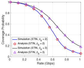
Now we verify the obtained rate coverage probability by comparing with the simulation results. In the verification, we assume the Rayleigh fading for the satellite and terrestrial links for simplicity. Note that the Shadowed-Rician fading reduces to the Rayleigh fading when , and the Nakagami fading reduces to the Rayleigh fading when . Despite the use of simplified fading, the analytical expressions regarding the geometries of the satellites and the terrestrial BSs can be properly validated. The system parameters used in the simulation are given in Table I, which are taken from [22, 20, 24]. As shown in Fig. 3, whose caption includes the system parameters not specified in Table I, Theorem 1 and the rate coverage probability obtained by numerical simulations match well.
V STIN Benefits Study: Coverage Extension and Data Offloading
Leveraging the derived analytical results, we explore the benefits that STINs provide in two different scenarios: coverage extension in remote rural areas and data offloading in dense urban areas. The used simulation parameters are same with Table I, unless specified otherwise. For the Shadowed-Rician channel parameter adopted in modeling the satellite, communications we refer Table II, which is taken from [31]. For the Nakagami channel parameter adopted for terrestrial communications, we assume .
| Scenarios | |||
|---|---|---|---|
| Frequent Heavy Shadowing (FHS) | |||
| Average Shadowing (AS) | |||
| Infrequent Light Shadowing (ILS) |
V-A Coverage Extension in Remote Rural Areas
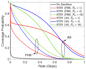
The deployment density of the terrestrial network is often limited, e.g., in a desert or in a deep mountain valley, resulting in users being left outside of coverage regions. In contrast to that, the satellite network provides a relatively consistent density as each satellite continues to move along a given orbit around the Earth. This is where the STIN is particularly useful, as it can provide coverage to the users experiencing outages in the terrestrial network. Our model can show how the coverage extension benefits are obtained as illustrated in Fig. 4. For clarity and brevity, we present only the FHS and AS scenarios of the Shadowed-Rician channels. The result of the ILS scenario is omitted since it is similar to that of the AS scenario.
In Fig. 4, we demonstrate significant improvements in the rate coverage by using the STIN. In particular, when is low (), the median rate (i.e., the rate that of the users can achieve) is Gbps when using the terrestrial network only. This implies that due to the scarcity of terrestrial BS’s deployment, of users are unable to be served. On the contrary, the STIN with achieves the median rate Gbps in the FHS scenario and Gbps in the AS scenario. As expected, we observe more significant rate coverage improvements in the AS scenario. One interesting observation is the trend of the rate coverage of the STIN is changed depending on the shadowing scenario. For instance, in the FHS scenario, the rate coverage steadily increases as increases up to . Conversely, in the AS scenario, the rate coverage starts to degrade when increases from to . This is attributed to the diminishing interference power in the presence of heavy shadowing. With lower interference power, densifying the satellite network leads to larger rate coverage improvements.
V-B Data Offloading in Dense Urban Areas
In dense urban areas where the data traffic load is high, the terrestrial network can suffer from scarcity of the available wireless resources. In the STIN, the satellite network is capable of relieving the traffic by data offloading. To capture this, adopting the approach used in HetNets [10, 11], we first redefine the rate by incorporating the load as follows:
| (53) |
where is the load relevant to the network type with Inspired by the mean load characterization in [10], we approximate the load as follows:
| (54) |
Incorporating the load, the rate coverage probability is given by
| (55) |
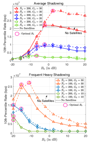
We explore the data offloading in the STIN by describing the th-percentile rate (the rate that of the users can achieve) in Fig. 5 depending on , , and . In Fig. 5 under the AS scenario, we observe that the STIN with , achieves around bps at . It corresponds to gains by comparing to the no satellites case. These gains come from that the load balancing effect, which has been mainly investigated in HetNets [10, 11], is also attained in the STIN. To be specific, if no satellites are used, all the users are associated with the terrestrial network. This increases the load and decreases the available resources per user . This eventually degrades the rate coverage performance. In the STIN, the users are associated with either the terrestrial or the satellite network, which makes the total load be balanced into and . This brings the offloading gains. We observe the offloading gains in the FHS scenario as well. In Fig. 5 under the FHS scenario, the STIN with , achieves around gains by comparing to the no satellites case. The offloading gains are eroded compared to the AS scenario because of the heavy shadowing. Due to the heavy shadowing, the signal power of the satellites diminishes, resulting in that the SINR of the satellite network degrades.
It is worthwhile to mention that careful design of the biasing factor is necessary to obtain the offloading gains. The biasing factor has a role to control the user populations connected to the satellite network. On the one hand, if is too small, then most of the users are connected to the terrestrial network; which does not help to balance the load. On the other hand, if is too large, too many users are connected to the satellite network, so that the users suffer from low rate. Accordingly, using a proper is crucial to optimally balance the load. In addition to this, high beamforming gains are also required in the satellite network to achieve the offloading gains. To efficiently perform the offloading, the density of the satellite network should be on par with that of the terrestrial network. However, since the satellite network is much more vulnerable to the interference compared to the terrestrial network [24], the rate performance of the satellite network severely deteriorates as its density increases. To compensate this, the satellite network needs high desired beamforming gains compared to that of the terrestrial network. In summary, achieving offloading gains in the STIN hinges on two critical factors: the appropriate setting of the biasing factor and sufficiently high beamforming gains in the satellite networks.
VI Conclusions
In this paper, we have developed a unified modeling for the two components of a STIN. Our key idea for capturing both of the satellite network and the terrestrial network into one framework is distributing PPPs on spheres and assigning random heights. Based on this model, we have derived the rate coverage probability as a function of the key system parameters, chiefly the densities, path-loss exponents, height geometries (maximum/minimum altitudes and height distributions), and bias factors of the satellites and the terrestrial BSs. Leveraging the analysis, we have explored the two benefits of the STIN: coverage extension in remote rural areas and data offloading in dense urban areas. Through this, we have extracted valuable system design insights: 1) In remote rural areas, the STIN significantly increases the rate coverage performance; yet to obtain this, it is necessary to carefully choose the satellite density. 2) In dense urban areas, the STIN helps to offload the data traffic from the terrestrial BSs; yet high enough beamforming gains of the satellites and proper bias are necessary.
Appendix A Proof of Lemma 1
We first recall that satellite at (with height ) is visible at the typical user if and only if (or equivalently ). For simplicity, we write . Let where is the height of satellite at , then represents the number of visible satellites. For , the probability generating function (PGF) of is
| (56) | |||
| (57) |
where (a) comes from the Laplace functional of an independently marked PPP and is the CDF of satellite height . Hence is Poisson with parameter , we have
| (58) |
This completes the proof.
Appendix B Proof of Lemma 2
Denoting by the nearest satellite distance to the typical user, the event is equivalent to the event that there is no satellite with a height in . Denoting as a set of satellites with height , we represent the CCDF of conditioned on the fact that at least one satellite is visible to the typical user as
| (61) |
where (a) follows from the fact that the PPP in and are independent since their sets do not overlap. Now we compute the first term in the numerator of (61) as
| (62) | |||
| (63) |
where is an area function of made feasible for the whole region of , defined as (34). The second term in the numerator of (61) is
| (64) |
where is (34). Now we put (63) and (64) together, which leads to
| (67) |
We finally derive the conditional PDF. Since the conditional PDF is obtained by taking derivative to the conditional CDF regarding , we have
| (68) |
where is the derivative of with regard to obtained as
| (69) |
if and otherwise. Plugging (69) into (68), we reach
| (70) |
where and are defined in (35). Noting that the distance can have a feasible range of as defined in (36), we complete the proof.
Appendix C Proof of Lemma 3
The typical user is connected to the satellite network when a satellite provides the maximum reference signal power, i.e., Calculating the above probability, we get
| (71) |
The inner probability of (71) is equivalent to the probability that there is no terrestrial BS whose distance to the typical user is smaller than . We compute this as follows. Denoting that a set of terrestrial BSs whose heights are in as and , is a homogeneous PPP with the density of , where . Further, and are statistically independent if . Hence, for given , the inner probability of (71) is
| (72) |
where (a) comes from Riemann integration with and is an extended area function of defined in (40) The final step is marginalizing (72) with regard to . Since is distributed as (32), we reach
| (73) |
This completes the proof.
Appendix D Proof of Lemma 5
Conditioned on that the distance to the interference source is larger than , the aggregated satellite interference is . We first note that the aggregated satellite interference can be further separated into where represents the interference coming from the satellites with height and . We note that and are independent for due to independent thinning of a PPP. Accordingly, the conditional Laplace transform is written as
| (74) |
Then we have
| (75) | |||
| (76) | |||
| (77) |
where (a) comes from the probability generating functional (PGFL) of a PPP, (b) follows the moment generating function (MGF) of the Shadowed-Rician fading power . Further, . Combining all , we reach
| (78) |
where and . Next, we obtain the conditional Laplace transform of the aggregated terrestrial interference. Due to the space limitation, we briefly present the result as follows. The proof technique is fundamentally equivalent to the satellite interference case. Conditioned on that the distance to the interference source is larger than , the conditional Laplace transform of the aggregated terrestrial interference is
| (79) |
where (a) comes from the MGF of the Nakagami- fading power, and .
Appendix E Proof of Theorem 1
We recall that the rate coverage probability is expressed as
| (80) | |||
| (81) |
Conditioned on that the typical user is associated with the satellite network, the SINR is
| (82) |
where , , and . We also have , , and . Note that the conditional rate coverage probability is
| (83) |
where and the expectation is taken over the randomness associated with . Since the CDF of the Shadowed-Rician fading power is obtained as
| (84) |
where . Since , we have
| (85) |
where . Next, we obtain the rate coverage probability under the condition that the typical user is associated with the terrestrial network. Similar to the satellite network association case, we have
| (86) |
where , , and , with , , and . The rate coverage probability for the terrestrial network association case is , which gives
| (87) |
where . Since the expectation in (87) is associated with the conditional nearest terrestrial BS’s distance whose PDF is obtained in Corollary 3. Eventually, we reach (52). This completes the proof.
References
- [1] J. C. McDowell, “The low earth orbit satellite population and impacts of the SpaceX Starlink constellation,” The Astrophysical Journal Letters, vol. 892, no. 2, p. L36, apr 2020.
- [2] J. P. Choi and C. Joo, “Challenges for efficient and seamless space-terrestrial heterogeneous networks,” IEEE Commun. Mag., vol. 53, no. 5, pp. 156–162, 2015.
- [3] H. Yao, L. Wang, X. Wang, Z. Lu, and Y. Liu, “The space-terrestrial integrated network: An overview,” IEEE Commun. Mag., vol. 56, no. 9, pp. 178–185, 2018.
- [4] P. Wang, J. Zhang, X. Zhang, Z. Yan, B. G. Evans, and W. Wang, “Convergence of satellite and terrestrial networks: A comprehensive survey,” IEEE Access, vol. 8, pp. 5550–5588, 2020.
- [5] B. Di, H. Zhang, L. Song, Y. Li, and G. Y. Li, “Ultra-dense LEO: Integrating terrestrial-satellite networks into 5G and beyond for data offloading,” IEEE Trans. Wireless Commun., vol. 18, no. 1, pp. 47–62, 2019.
- [6] W. Abderrahim, O. Amin, M.-S. Alouini, and B. Shihada, “Proactive traffic offloading in dynamic integrated multisatellite terrestrial networks,” IEEE Trans. Commun., vol. 70, no. 7, pp. 4671–4686, 2022.
- [7] D. Wang, W. Wang, Y. Kang, and Z. Han, “Distributed data offloading in ultra-dense LEO satellite networks: A Stackelberg mean-field game approach,” IEEE J. Sel. Topics Signal Process., vol. 17, no. 1, pp. 112–127, 2023.
- [8] F. Baccelli and B. Blaszczyszyn, “Stochastic geometry and wireless networks: Volume i theory,” Found. Trends in Networking, vol. 3, no. 3–4, p. 249–449, Mar. 2009.
- [9] M. Haenggi, J. G. Andrews, F. Baccelli, O. Dousse, and M. Franceschetti, “Stochastic geometry and random graphs for the analysis and design of wireless networks,” IEEE J. Sel. Areas Commun., vol. 27, no. 7, pp. 1029–1046, 2009.
- [10] S. Singh, H. S. Dhillon, and J. G. Andrews, “Offloading in heterogeneous networks: Modeling, analysis, and design insights,” IEEE Trans. Wireless Commun., vol. 12, no. 5, pp. 2484–2497, 2013.
- [11] S. Singh and J. G. Andrews, “Joint resource partitioning and offloading in heterogeneous cellular networks,” IEEE Trans. Wireless Commun., vol. 13, no. 2, pp. 888–901, 2014.
- [12] J. Park, N. Lee, J. G. Andrews, and R. W. Heath, “On the optimal feedback rate in interference-limited multi-antenna cellular systems,” IEEE Trans. Wireless Commun., vol. 15, no. 8, pp. 5748–5762, 2016.
- [13] N. Lee, D. Morales-Jimenez, A. Lozano, and R. W. Heath, “Spectral efficiency of dynamic coordinated beamforming: A stochastic geometry approach,” IEEE Trans. Wireless Commun., vol. 14, no. 1, pp. 230–241, 2015.
- [14] T. Bai, A. Alkhateeb, and R. W. Heath, “Coverage and capacity of millimeter-wave cellular networks,” IEEE Commun. Mag., vol. 52, no. 9, pp. 70–77, 2014.
- [15] J. Park, J. G. Andrews, and R. W. Heath, “Inter-operator base station coordination in spectrum-shared millimeter wave cellular networks,” IEEE Trans. Cognitive Commun. and Networking, vol. 4, no. 3, pp. 513–528, 2018.
- [16] V. V. Chetlur and H. S. Dhillon, “Downlink coverage analysis for a finite 3-D wireless network of unmanned aerial vehicles,” IEEE Trans. Commun., vol. 65, no. 10, pp. 4543–4558, 2017.
- [17] M. Banagar and H. S. Dhillon, “Performance characterization of canonical mobility models in drone cellular networks,” IEEE Trans. Wireless Commun., vol. 19, no. 7, pp. 4994–5009, 2020.
- [18] A. Al-Hourani, “An analytic approach for modeling the coverage performance of dense satellite networks,” IEEE Wireless Commun. Lett., vol. 10, no. 4, pp. 897–901, 2021.
- [19] ——, “Optimal satellite constellation altitude for maximal coverage,” IEEE Wireless Commun. Lett., vol. 10, no. 7, pp. 1444–1448, 2021.
- [20] N. Okati, T. Riihonen, D. Korpi, I. Angervuori, and R. Wichman, “Downlink coverage and rate analysis of low Earth orbit satellite constellations using stochastic geometry,” IEEE Trans. Commun., vol. 68, no. 8, pp. 5120–5134, 2020.
- [21] N. Okati and T. Riihonen, “Nonhomogeneous stochastic geometry analysis of massive LEO communication constellations,” IEEE Trans. Commun., vol. 70, no. 3, pp. 1848–1860, 2022.
- [22] D.-H. Jung, J.-G. Ryu, W.-J. Byun, and J. Choi, “Performance analysis of satellite communication system under the shadowed-Rician fading: A stochastic geometry approach,” IEEE Trans. Commun., vol. 70, no. 4, pp. 2707–2721, 2022.
- [23] D.-H. Na, K.-H. Park, Y.-C. Ko, and M.-S. Alouini, “Performance analysis of satellite communication systems with randomly located ground users,” IEEE Trans. Wireless Commun., vol. 21, no. 1, pp. 621–634, 2022.
- [24] J. Park, J. Choi, and N. Lee, “A tractable approach to coverage analysis in downlink satellite networks,” IEEE Trans. Wireless Commun., vol. 22, no. 2, pp. 793–807, 2023.
- [25] Z. Song, J. An, G. Pan, S. Wang, H. Zhang, Y. Chen, and M.-S. Alouini, “Cooperative satellite-aerial-terrestrial systems: A stochastic geometry model,” IEEE Trans. Wireless Commun., vol. 22, no. 1, pp. 220–236, 2023.
- [26] B. A. Homssi and A. Al-Hourani, “Modeling uplink coverage performance in hybrid satellite-terrestrial networks,” IEEE Commun. Lett., vol. 25, no. 10, pp. 3239–3243, 2021.
- [27] Y. Tian, G. Pan, H. ElSawy, and M.-S. Alouini, “Satellite-aerial communications with multi-aircraft interference,” IEEE Trans. Wireless Commun., vol. 22, no. 10, pp. 7008–7024, 2023.
- [28] H. Zhang, C. Du, S. Wang, G. Pan, and J. An, “Effects of spatially random space interference on satellite-aerial downlink transmission,” IEEE Trans. Commun., vol. 70, no. 7, pp. 4956–4971, 2022.
- [29] Y. Tian, G. Pan, M. A. Kishk, and M.-S. Alouini, “Stochastic analysis of cooperative satellite-UAV communications,” IEEE Trans. Wireless Commun., vol. 21, no. 6, pp. 3570–3586, 2022.
- [30] H. Cundy and A. Rollett, “Sphere and cylinder—-Archimedes’ theorem,” Mathematical Models, pp. 172–173, 1989.
- [31] A. Abdi, W. Lau, M.-S. Alouini, and M. Kaveh, “A new simple model for land mobile satellite channels: first- and second-order statistics,” IEEE Trans. Wireless Commun., vol. 2, no. 3, pp. 519–528, 2003.
- [32] M. Di Renzo, “Stochastic geometry modeling and analysis of multi-tier millimeter wave cellular networks,” IEEE Trans. Wireless Commun., vol. 14, no. 9, pp. 5038–5057, 2015.
- [33] J. G. Andrews, F. Baccelli, and R. K. Ganti, “A tractable approach to coverage and rate in cellular networks,” IEEE Trans. Commun., vol. 59, no. 11, pp. 3122–3134, 2011.
- [34] D. Kim, J. Park, and N. Lee, “Coverage analysis of dynamic coordinated beamforming for leo satellite downlink networks,” ArXiv, 2023. [Online]. Available: https://arxiv.org/abs/2309.10460
- [35] J. Park, N. Lee, and R. W. Heath, “Feedback design for multi-antenna -tier heterogeneous downlink cellular networks,” IEEE Trans. Wireless Commun., vol. 17, no. 6, pp. 3861–3876, 2018.