Calibrating Car-Following Models via Bayesian Dynamic Regression

Abstract

Car-following behavior modeling is critical for understanding traffic flow dynamics and developing high-fidelity microscopic simulation models. Most existing impulse-response car-following models prioritize computational efficiency and interpretability by using a parsimonious nonlinear function based on immediate preceding state observations. However, this approach disregards historical information, limiting its ability to explain real-world driving data. Consequently, serially correlated residuals are commonly observed when calibrating these models with actual trajectory data, hindering their ability to capture complex and stochastic phenomena. To address this limitation, we propose a dynamic regression framework incorporating time series models, such as autoregressive processes, to capture error dynamics. This statistically rigorous calibration outperforms the simple assumption of independent errors and enables more accurate simulation and prediction by leveraging higher-order historical information. We validate the effectiveness of our framework using HighD and OpenACC data, demonstrating improved probabilistic simulations. In summary, our framework preserves the parsimonious nature of traditional car-following models while offering enhanced probabilistic simulations. The code of this work is open-sourced at https://github.com/Chengyuan-Zhang/IDM_Bayesian_Calibration.

Keywords: Car-Following Models, Dynamic Regression, Bayesian Inference, Microscopic Traffic Simulation

1 Introduction

Car-following behavior plays a critical role in understanding and predicting traffic flow dynamics. Various car-following models have been developed in the literature, including the optimal speed model (OVM) (Bando et al., 1995), Gipps model (Gipps, 1981), and the intelligent driver model (IDM) (Treiber et al., 2000) along with its variants (Treiber and Helbing, 2003; Derbel et al., 2012). These models typically utilize recent observations of the ego vehicle’s speed, relative speed to the leading vehicle, and spacing/gap as inputs to a explicitly predefined nonlinear function. This function computes the acceleration or speed as the driver’s decision at the current time step. The parsimonious structure of these models offers computational efficiency, interpretability, and analytical connections with macroscopic relations (Treiber et al., 2010). Consequently, car-following model-based simulations have been widely used to gain insights into complex traffic flow dynamics.

Despite the fact that car-following models can reproduce important physical phenomena such as shockwaves, it has been highlighted in many recent studies that their parsimonious structure limits the effectiveness of reproducing real-world driving behaviors with high fidelity (Wang et al., 2017). The simplicity of these parsimonious models overlooks high-order historical information, resulting in inaccurate predictions. Recent studies have shown that incorporating observations from the past $1\sim 4$ seconds improves the modeling of car-following decisions (Zhang and Sun, 2022). However, calibrating parsimonious car-following models based on single-timestamp observations from real-world trajectories leads to temporally correlated errors. Assuming independent errors in the calibration process introduces bias (Hoogendoorn and Hoogendoorn, 2010). To address this challenge, Zhang and Sun (2022) developed a Bayesian calibration framework by modeling errors using Gaussian processes (GPs). Although this approach offers improved and consistent calibration, it is not a flexible solution for simulation due to the computational complexity of the predictive mechanism of GPs.

Although these models are valuable in understanding traffic flow dynamics, the limitations suggest a need for a more nuanced approach to address the biased calibration of existing car-following models. In this paper, we utilize a dynamic regression framework to model car-following sequence data, incorporating a generative time series model to capture errors. The proposed framework builds upon the classic car-following model, i.e., IDM, retaining the parsimonious features of traditional car-following models while significantly improving prediction accuracy and enabling probabilistic simulations by incorporating higher-order historical information. Here we emphasize that our framework doesn’t change the parsimonious structure of the existing models and thus can be applied to various car-following models. The experiments demonstrate the effectiveness of this framework in achieving enhanced predictions and a more accurate calibration of the car-following models. Our results suggest that the driving actions within the past 10 seconds should be considered when modeling human car-following behaviors. This aligns with the literature (Wang et al., 2017) where 10-s historical information is testified as the best input.

The contributions of this work are threefold:

1. We present a novel calibration method for car-following models based on a dynamic regression framework. This method enhances existing parsimonious car-following models by incorporating higher-order historical information without changing the prevailing models. The inclusion of this flexible form enables unbiased calibration.

2. The framework integrates autoregressive (AR) processes within time series models to handle errors, representing an advancement from the conventional assumption of independent and identically distributed (i.i.d.) errors. This enhancement introduces a statistically rigorous approach, offering improved modeling capabilities.

3. The data generative processes of our framework offer an efficient probabilistic simulation method for car-following models, which reasonably involves the stochastic nature of human driving behaviors and accurately replicates real-world traffic phenomena.

This paper is organized as follows. Section 2 overviews the existing car-following models and simulation methods. Section 3 introduces our proposed dynamic regression framework to address the limitations of existing models. Section 4 demonstrates the effectiveness of our model in calibration and simulation, followed by conclusions in Section 5.

2 Related Works

Car-following models have been extensively used to understand and predict drivers’ behaviors in traffic, and model calibration is crucial. The traditional calibration methods, such as genetic algorithm-based calibration (Punzo et al., 2021), provide only point estimation for model parameters, lacking the ability to capture driving behavior uncertainty. In contrast, probabilistic calibration and modeling approaches are commonly considered effective in addressing both epistemic uncertainties related to unmodeled details and aleatory uncertainty resulting from the model prediction failures (Punzo et al., 2012).

A well-designed car-following model should capture both the inter-driver heterogeneity (diverse driving behaviors of different drivers (Ossen et al., 2006)) and intra-driver heterogeneity (the varying driving styles of the same driver (Taylor et al., 2015)). Probabilistic calibration collects significant data from various drivers and conditions to fit the model parameters using statistical distributions instead of fixed values. For instance, the IDM parameters like comfortable deceleration and maximum acceleration can be modeled as random variables with specific distributions (Treiber and Kesting, 2017; Zhang and Sun, 2022), reflecting the range of driving styles. A typical probabilistic calibration method is maximum likelihood estimation (MLE) (Treiber and Kesting, 2013b; Zhou et al., 2023). Bayesian inference, as another probabilistic approach, combines prior knowledge and data to estimate the model parameter distribution, allowing for capturing inter-driver heterogeneity. By representing behaviors probabilistically, a spectrum of plausible behaviors is obtained instead of a single deterministic response. Bayesian calibration approaches are discussed in detail in Zhang and Sun (2022). To address intra-driver heterogeneity, stochastic car-following models are developed to account for a driver’s behavior’s dynamic, time-varying nature. These models introduce a random component that captures moment-to-moment behavior changes, such as using a stochastic process like Markov Chain to model a driver’s reaction time or attention level. For instance, Zhang et al. (2022) modeled each IDM parameter as a stochastic process and calibrated them in a time-varying manner.

In addition to traditional models, machine learning techniques have gained popularity in driving behavior modeling and prediction. These techniques leverage large datasets to capture complex, non-linear relationships and account for inter-driver and intra-driver heterogeneity. Data-driven models can be trained on a wealth of driving data to predict individual driver behavior and traffic flow, such as K-nearest neighbor algorithm (KNN) (He et al., 2015), Gaussian mixture model (GMM) (Lefèvre et al., 2014), hidden Markov model (HMM) (Wang et al., 2018), and long short-term memory (LSTM) networks (Wang et al., 2017). These models can complement traditional car-following models and enhance their predictive capabilities. Furthermore, the real-time adaptation of model parameters based on the current driving context and state of the driver and the vehicle can capture intra-driver heterogeneity. This involves continuous parameter updates using sensory information to reflect changes in driving conditions (Sun et al., 2022).

Overall, probabilistic car-following models, enhanced by machine learning and real-time adaptation, offer a robust framework for capturing the observed diverse and complex driving behaviors. These models effectively handle the heterogeneity and uncertainty inherent in driving behavior by leveraging various methodologies. However, each model has its limitations. While data-driven models can capture complex patterns, they may lack interpretability and be data-hungry. They can also be prone to the out-of-distribution problem. Traditional car-following models, though transparent, may not be flexible enough to encompass the full complexity of human driving behaviors. This work aims to leverage the prior knowledge of traditional car-following models while incorporating the flexibility needed to represent diverse human driving behaviors accurately. The efficacy of this approach is explicitly demonstrated through calibration and simulations of the IDM.

3 Methodology

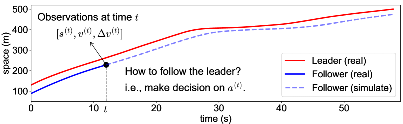
Figure 1: Illustration of the car-following problem in the time-spacing diagram.

3.1 Preliminaries: IDM and its Variants

In this part, we assume that the internal states of each driver remain stationary, implying that their driving styles do not change within the region of interest (ROI). Thus we ignore the discussion of intra-driver heterogeneity. This assumption allows us to use a single model with time-invariant parameters to learn observed car-following behaviors. As a starting point, we introduce several models: the basic IDM with a deterministic formulation (Treiber et al., 2000), the probabilistic IDM with action uncertainty (Treiber and Kesting, 2017), the Bayesian IDM with prior knowledge, and the memory-augmented IDM with a temporal structure (Zhang and Sun, 2022).

3.1.1 Intelligent Driver Model

IDM (Treiber et al., 2000) is a continuous nonlinear function $f:\mathbb{R}^{3}\mapsto\mathbb{R}$ which maps the gap, the speed, and the speed difference (approach rate) to acceleration at a certain timestamp. Let $s$ represent the gap between the following vehicle and the leading vehicle, $v$ denote the following vehicle’s speed, and $\Delta v=-ds/dt$ indicate the speed difference. The physical meanings of these notations are illustrated in Figure 1, where $v_{l}$ denotes the speed of the leading vehicle. IDM computes vehicle acceleration using the following nonlinear function $f$:

$$\begin{split}f(s,v,\Delta v)\triangleq\alpha\,\left(1-\left({\frac{v}{v_{0}}}\right)^{4}-\left({\frac{s^{\ast}(v,\Delta v)}{s}}\right)^{2}\right),\end{split}$$ (1)

$$\begin{split}s^{\ast}(v,\Delta v)=s_{0}+s_{1}\,\sqrt{\frac{v}{v_{0}}}+v\,T+{\frac{v\,\Delta v}{2\,{\sqrt{\alpha\,\beta}}}},\end{split}$$ (2)

where $v_{0},s_{0},T,\alpha,$ and $\beta,$ are model parameters with specific physical meanings. The desired speed $v_{0}$ is the free-flow speed. The jam spacing $s_{0}$ denotes a minimum gap distance from the leading vehicle. The safe time headway $T$ represents the minimum interval between the following and leading vehicles. The acceleration $\alpha$ and the comfortable braking deceleration $\beta$ are the maximum vehicle acceleration and the desired deceleration to keep safe, respectively. The deceleration is controlled by the desired minimum gap $s^{\ast}$, and we set $s_{1}=0$ following Treiber et al. (2000) to obtain a model with interpretable and easily measurable parameters.

To make the notations concise and compact, we define a vector $\bm{\theta}=[v_{0},s_{0},T,\alpha,\beta]\in\mathbb{R}^{5}$ as the IDM parameters. For a certain driver $d$, we formulate the IDM acceleration term as $f(s_{d}^{(t)},v_{d}^{(t)},\Delta v_{d}^{(t)};\bm{\theta}_{d})$. Compactly, we write the inputs at time $t$ as a vector $\bm{h}_{d}^{(t)}=[s_{d}^{(t)},v_{d}^{(t)},\Delta v_{d}^{(t)}]$. Then, we denote the IDM term as $\mathrm{IDM}^{(t)}(\bm{h}_{d}^{(t)};\bm{\theta}_{d})$, further abbreviated as $\mathrm{IDM}_{d}^{(t)}$, where the subscript $d$ represents the index for each driver and the superscript $(t)$ indicates the timestamp. Given $\mathrm{IDM}_{d}^{(t)}$, we can update the vehicle speed $v^{(t+1)}$ and position $x^{(t+1)}$ following the ballistic integration scheme as in Treiber and Kesting (2013a) with a step of $\Delta t$:

$$v^{(t+1)} =v^{(t)}+a^{(t)}\Delta t,$$ (3a)

$$x^{(t+1)} =x^{(t)}+v^{(t)}\Delta t+\frac{1}{2}a^{(t)}\Delta t^{2}.$$ (3b)

Specifically, three steps are involved in the discrete decision-making processes simulation shown in Equation 3. (i) Initialization: the available information at time $t$ includes $a^{(t-1)}$, $x^{(t)}$, and $v^{(t)}$; (ii) Decision-making: we estimate the possible action $\mathrm{IDM}^{(t)}$ based on IDM; (iii) Action execution and state updates: We take a specific action $a^{(t)}$ according to the decisions, resulting in the updated motion states $v^{(t+1)}$ (Equation 3a) and $x^{(t+1)}$ (Equation 3b). The calibration of IDM can be performed using different data, such as spacing, speed, and acceleration, as outlined in Punzo et al. (2021). In this section, we focus on introducing the generative processes of acceleration data and provide detailed calibration methods on the speed or/and spacing in Section 3.2.

Figure 2: The decision-action simulation scheme.

3.1.2 Probabilistic IDM with i.i.d. Errors

Imperfect and irregular driving behaviors result in erratic components of the driver’s action (Treiber and Kesting, 2013b; Saifuzzaman and Zheng, 2014). We can introduce some action noises with standard deviations $\sigma_{\eta}$ that are tolerated in the IDM framework to model such behaviors. Here, $a_{\text{IDM}}$ represents the rational behavior model, while the random term accounts for the imperfect driving behaviors that IDM cannot capture. Considering the random term with the assumption of i.i.d. noise, a probabilistic IDM (Bhattacharyya et al., 2020; Treiber and Kesting, 2017) can be developed as

$$\hat{a}_{d}^{(t)}|\bm{h}_{d}^{(t)},\bm{\theta}_{d}\,\stackon{\sim}{\tiny{\textit{i.i.d.}}}\,\mathcal{N}(\mathrm{IDM}_{d}^{(t)},\sigma_{\eta}^{2}),$$ (4)

where $\mathrm{IDM}$ and $\sigma^{2}_{\eta}$ represent the mean and variance and $\hat{a}$ is the observed data of the true acceleration ${a}$.

The car-following model calibration is to estimate the model parameters $\bm{\theta}$ by seeking the best mapping from $\bm{h}_{d}^{(t)}$ to $a_{d}^{(t)}$, ${v}_{d}^{(t+1)}$, and $s_{d}^{(t+1)}$ (Punzo et al., 2021). Various approaches, such as utility-based optimization and maximum-likelihood techniques, are usually adopted (see Treiber and Kesting (2013a)).

3.1.3 Bayesian IDM with i.i.d. Errors

We introduce a hierarchical Bayesian IDM, as proposed by Zhang and Sun (2022), that explicitly captures general driving behaviors at the population level while representing individual-level heterogeneity. This model is described as follows: For any pairs of time step and vehicle $(t,d)$ in the set $\{(t,d)\}_{t=t_{0},d=1}^{t_{0}+T\Delta t,D}$, we have

$$\bm{\sigma}_{0} \sim\mathrm{Exp}(\lambda_{0}),$$ (5a)

$$\bm{\Sigma} \sim\mathrm{LKJCholeskyCov}(\eta,\bm{\sigma}_{0}),$$ (5b)

$$\ln(\bm{\theta}) \sim\mathcal{N}(\bm{0},\bm{\Sigma}_{0}),$$ (5c)

$$\ln(\bm{\theta}_{d}) \sim\mathcal{N}(\ln(\bm{\theta}),\bm{\Sigma}),$$ (5d)

$$\sigma_{\eta} \sim\mathrm{Exp}(\lambda_{\eta}),$$ (5e)

$$\hat{a}_{d}^{(t)}|\bm{h}_{d}^{(t)},\bm{\theta}_{d}\, \stackon{$\sim$}{\tiny{\textit{i.i.d.}}}\,\mathcal{N}(\mathrm{IDM}_{d}^{(t)},\sigma_{\eta}^{2}),$$ (5f)

where LKJ represents the LKJ distribution (Lewandowski et al., 2009), $\lambda_{0}$, $\eta$, $\bm{\Sigma}_{0}$, and $\lambda_{\eta}$ are the manually set hyperparameters, and the other variables are inferred from the data. However, note that Equation 5f assumes i.i.d. errors, but in practice, the residuals are temporally correlated, i.e., non-i.i.d., as illustrated in Figure 3.

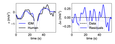
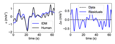
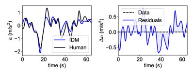
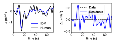
Figure 3: Examples of the non-i.i.d. residuals of the Bayesian IDM for four leader-follower pairs, where the left ones indicate the actual acceleration profiles v.s. the IDM term with identified parameters, the right ones are the residuals between the real data and the IDM term.

3.1.4 Memory-Augmented IDM with Gaussian Processes and i.i.d. Errors

Maintaining temporal consistency in actions in daily driving tasks is crucial for human drivers, commonly referred to as driving persistence (Treiber and Kesting, 2013b). However, most stochastic models, including the Bayesian IDM, overlook the persistence of acceleration noise. Instead, they incorrectly model its time dependence as white noise, assuming i.i.d. errors, as shown in Equation 4, which can be reformulated as

$$a_{d}^{(t)}=\mathrm{IDM}_{d}^{(t)}+\epsilon_{d}^{(t)},\ \epsilon_{d}^{(t)}\,\stackon{\sim}{\tiny{\emph{i.i.d.}}}\,\mathcal{N}(0,\sigma_{\eta}^{2}).$$ (6)

Actually, these models and calibrated parameters are only valid when the errors adhere to the i.i.d. assumption, and the temporal correlation in residuals leads to biased estimation of model parameters.

To address this limitation, Zhang and Sun (2022) proposed a Bayesian calibration method that involves Gaussian processes (GPs) to depict the “memory effect” (Treiber and Helbing, 2003), named as memory-augmented IDM (MA-IDM), which can capture the temporally correlated errors, $a_{d}^{(t)}=\mathrm{IDM}_{d}^{(t)}+a_{\mathrm{GP}\,d}^{(t)}$. Stacking the scalar $a_{d}^{(t)}$ along the time horizon $\forall t\in[t_{0}+\Delta t,t_{0}+T\Delta t]$ results in a vector $\bm{a}_{d}\in\mathbb{R}^{T}$. Such that we can derive a vector form $\bm{a}_{d}=\mathrm{\textbf{IDM}}_{d}+\bm{a}_{\mathrm{GP}\,d}$, with $\bm{a}_{\mathrm{GP}\,d}\sim\mathcal{N}(\bm{0},\bm{K})$, where $\bm{K}$ represents the kernel matrix constructed by radial basis function (RBF) kernel with $\sigma_{k}$ and $\ell$. With this setting, the MA-IDM is written as

$$\bm{\sigma}_{0} \sim\mathrm{Exp}(\lambda_{0}),$$ (7a)

$$\bm{\Sigma} \sim\mathrm{LKJCholeskyCov}(\eta,\bm{\sigma}_{0}),$$ (7b)

$$\ln(\bm{\theta}) \sim\mathcal{N}(\bm{0},\bm{\Sigma}_{0}),$$ (7c)

$$\ln(\bm{\theta}_{d}) \sim\mathcal{N}(\ln(\bm{\theta}),\bm{\Sigma}),$$ (7d)

$$\sigma_{k} \sim\mathrm{Exp}(\lambda_{k}),$$ (7e)

$$\ln(\ell) \sim\mathcal{N}(\mu_{\ell},\sigma_{\ell}),$$ (7f)

$${\bm{a}}_{d}|\bm{h}_{d},\bm{\theta}_{d}\, \stackon{$\sim$}{\tiny{\textit{i.i.d.}}}\,\mathcal{N}\left(\mathrm{\textbf{IDM}}_{d},\bm{K}\right).$$ (7g)

3.2 Calibration of the Dynamic IDM with Autoregressive Processes and i.i.d. Errors

(a) Bayesian IDM.

(b) MA-IDM.

(c) Dynamic IDM.

Figure 4: Probabilistic graphical models.

The kernel function selection restricts the flexibility of modeling the temporally correlated errors with GPs. To address this limitation, we propose a novel unbiased hierarchical Bayesian model called dynamic IDM. This model addresses this limitation by incorporating AR processes to represent the time-dependent stochastic error term with a dynamic regression framework. By absorbing AR processes in the calibration framework, we adopt a simple yet effective approach of adding up actions along the history steps. This approach has been tested and proven effective in modeling car-following behaviors (Ma and Andréasson, 2005).

Here we distinguish the concepts of “states” and “observations”, where states (i.e., the real acceleration) representing the underlying dynamics of the vehicle, and observations are the measured values (e.g., speed and spacing). In Section 3.2.1, we first build the equation of states, which describes how the system evolves along the time horizon. Then in the rest of this subsection, we develop the observation equation, which describes how the underlying state is transformed (with noise added) into something that we directly measure.

3.2.1 Modeling the temporal correlations with AR processes

Specifically, we assume the error of the state follows a $p$-order AR process denoted by $\mathrm{AR}(p)$:

$$a_{d}^{(t)} =\mathrm{IDM}_{d}^{(t)}+\epsilon^{(t)}_{d},$$ (8)

$$\epsilon^{(t)}_{d} =\rho_{1}\epsilon_{d}^{(t-1)}+\rho_{2}\epsilon_{d}^{(t-2)}+\dots+\rho_{p}\epsilon_{d}^{(t-p)}+\eta_{d}^{(t)},$$ (9)

where $\eta^{(t)}\,\stackon{$\sim$}{\tiny{\textit{i.i.d.}}}\mathcal{N}(0,\sigma_{\eta}^{2})$ represents a white noise series. In the following discussions, we refer to $\mathrm{IDM}_{d}^{(t)}$ as the mean component and $\epsilon^{(t)}_{d}$ as the stochastic component.

We estimate the model (Equation 8) by constructing the likelihood on a white noise process $\eta_{d}^{(t)}$. Given the model with estimated parameters, the probabilistic prediction can be achieved by first sampling $\eta_{d}^{(t)}$ and then sequentially feeding it into

$$a_{d}^{(t)}= \,\mathrm{IDM}_{d}^{(t)}+\rho_{1}(a_{d}^{(t-1)}-\mathrm{IDM}_{d}^{(t-1)})+\rho_{2}(a_{d}^{(t-2)}-\mathrm{IDM}_{d}^{(t-2)})+\cdots$$

$$\,+\rho_{p}(a_{d}^{(t-p)}-\mathrm{IDM}_{d}^{(t-p)})+\eta_{d}^{(t)}.$$ (10)

provides probabilistic prediction. The above equation explicitly demonstrates the advantages of our method compared with traditional models — it involves rich information from several historical steps to make decisions for the current step instead of using only one historical step.

Here, we introduce the form of the hierarchical dynamic IDM as $\forall(t,d)\in\{(t,d)\}_{t=t_{0},d=1}^{t_{0}+T\Delta t,D}$

$$\bm{\sigma}_{0} \sim\mathrm{Exp}(\lambda_{0}),$$ (11a)

$$\bm{\Sigma} \sim\mathrm{LKJCholeskyCov}(\eta,\bm{\sigma}_{0}),$$ (11b)

$$\ln(\bm{\theta}) \sim\mathcal{N}(\bm{0},\bm{\Sigma}_{0}),$$ (11c)

$$\ln(\bm{\theta}_{d}) \sim\mathcal{N}(\ln(\bm{\theta}),\bm{\Sigma}),$$ (11d)

$$\sigma_{\eta} \sim\mathrm{Exp}(\lambda_{\eta}),$$ (11e)

$$\bm{\rho} \sim\mathcal{N}(\bm{0},\mathrm{diag}(\bm{\sigma_{\rho}})),$$ (11f)

$${a}_{d}^{(t)}|\bm{h}_{d}^{(t)},\bm{\theta}_{d}\, \stackon{$\sim$}{\tiny{\textit{i.i.d.}}}\,\mathcal{N}\left(\mathrm{IDM}_{d}^{(t)}+\sum_{k=1}^{p}\rho_{k}\left(a_{d}^{(t-k)}-\mathrm{IDM}_{d}^{(t-k)}\right),\sigma_{\eta}^{2}\right),$$ (11g)

where $\bm{\rho}=[\rho_{1},\rho_{2},\dots,\rho_{p}]$ is estimated during model training. Given hyperparameters $\lambda_{0}$ and $\eta$, Equation 11a and Equation 11b set the prior for the covariance matrix $\bm{\Sigma}\in\mathbb{R}^{5}$ of the IDM parameters, which control the balance between the pooled model and the unpooled model, as highlighted by Zhang and Sun (2022). Then Equation 11c sets the prior for the population-level IDM parameters $\bm{\theta}$, and based on which Equation 11d describes the prior of the individual-level IDM parameters $\bm{\theta}_{d}$ for driver $d$. By providing the hyperparameter $\lambda_{\eta}$, we can specify the prior for the variance of the random noise in Equation 11e. Further, the priors of the AR coefficients are normally distributed with zero means, as shown in Equation 11f. Finally, we can derive the likelihood as a normal distribution shown in Equation 11g.

The Bayesian IDM is a special case of the dynamic IDM. If we set the AR order equal to zero (i.e., $p=0$), this model is exactly equivalent to the Bayesian IDM. We compare the probabilistic graphical models of the Bayesian IDM, MA-IDM, and dynamic IDM in Figure 4.

3.2.2 Calibration on speed data with observation noise

Our proposed method can be used for the calibration based on the acceleration, speed, and spacing data. Here, we provide a brief introduction to the calibration method based on speed data. More details could be found in the appendix.

According to Equation 3a, the likelihood of a noisy speed observation is written as

$$\hat{v}_{d}^{(t+1)}\sim\mathcal{N}\left(\bar{v}_{d}^{(t+1)},(\sigma_{\eta}\Delta t)^{2}+\sigma_{v}^{2}\right),$$ (12)

where $\bar{v}_{d}^{(t+1)}=v_{d}^{(t)}+\mathrm{IDM}_{d}^{(t)}\Delta t+\sum_{k=1}^{p}\rho_{k}\left(v_{d}^{(t-(k-1))}-v_{d}^{(t-k)}\right)-\sum_{k=1}^{p}\rho_{k}\mathrm{IDM}_{d}^{(t-k)}\Delta t$, $\hat{v}_{d}^{(t+1)}$ is the observed data of the true speed ${v}_{d}^{(t+1)}$, and $\sigma_{v}^{2}$ is the variance of the observation noise.

3.2.3 Calibration on position/spacing data with observation noise

According to Equation 3b, the likelihood of a noisy positional observation is written as

$$\hat{x}_{d}^{(t+1)}\sim\mathcal{N}\left(\bar{x}_{d}^{(t+1)},\Bigl{(}\frac{1}{2}\sigma_{\eta}\Delta t^{2}\Bigr{)}^{2}+\sigma_{x}^{2}\right),$$ (13)

where the mean $\bar{x}_{d}^{(t+1)}=x_{d}^{(t)}+v_{d}^{(t)}\Delta t+\frac{1}{2}\mathrm{IDM}_{d}^{(t)}\Delta t^{2}+\frac{1}{2}\sum_{k=1}^{p}\rho_{k}\left(v_{d}^{(t-(k-1))}-v_{d}^{(t-k)}\right)\Delta t-\frac{1}{2}\sum_{k=1}^{p}\rho_{k}\mathrm{IDM}_{d}^{(t-k)}\Delta t^{2}$, $\hat{x}_{d}^{(t+1)}$ is the observed data of the true position ${x}_{d}^{(t+1)}$, and $\sigma_{x}^{2}$ is the variance of the observation noise of position data. Note that this is a position-based form, but one can easily adapt it into a gap-based form.

3.2.4 Calibration on both speed and position data with joint likelihood

By jointly considering the information and observation noise from the speed and position data, we can derive the likelihood using a bi-variate normal distribution, written as

$$\left[\begin{array}[]{c}\hat{x}_{d}^{(t+1)}\\ \hat{v}_{d}^{(t+1)}\end{array}\right]\sim\mathcal{N}\left(\left[\begin{array}[]{c}\bar{x}_{d}^{(t+1)}\\ \bar{v}_{d}^{(t+1)}\end{array}\right],\left[\begin{array}[]{cc}\Bigl{(}\frac{1}{2}\sigma_{\eta}\Delta t^{2}\Bigr{)}^{2}&\frac{1}{2}\sigma_{\eta}^{2}\Delta t^{3}\\ \frac{1}{2}\sigma_{\eta}^{2}\Delta t^{3}&(\sigma_{\eta}\Delta t)^{2}\end{array}\right]+\left[\begin{array}[]{cc}\sigma_{x}^{2}&0\\ 0&\sigma_{v}^{2}\end{array}\right]\right).$$ (14)

The variance values ($\sigma_{x}$ and $\sigma_{v}$) in the observation noise determine the reliability of the position and speed data. When $\sigma_{x}$ is set to a large value, this form tends to be equal to pure calibration on the speed data. Similarly, when $\sigma_{v}$ is large, it equals calibration only using the position data.

4 Experiments and Simulations

We begin by evaluating the calibration results on the regression task and analyzing the identified parameters of IDM and the learned AR processes. Next, we demonstrate the simulation capability of our proposed method through short-term and long-term simulations. The short-term simulations quantitatively assess the replication of human behaviors, while the long-term simulations validate the ability of the identified parameters to capture critical car-following dynamics.

4.1 Experimental Settings

4.1.1 Dataset

The car-following model performance can be affected by noise in empirical data (Montanino and Punzo, 2015). To mitigate the impact of data quality and avoid the need for excessive data filtering, selecting an appropriate dataset is crucial. Different datasets can be utilized to verify various aspects of model capability. For instance, studying general car-following behaviors based on deep learning models requires informative data with sufficiently long trajectories. Exploring both population-level and individual-level driving behaviors based on hierarchical models necessitates multi-user driving data. Similarly, analyzing the driving style shifts in a single driver based on behavior models relies on the daily trajectories of that specific driver.

To access hierarchical car-following models for multiple drivers, we evaluate our model using the HighD dataset (Krajewski et al., 2018), which offers high-resolution trajectory data collected with drones. The HighD dataset provides several advantages over the NGSIM dataset (Punzo et al., 2011) with advanced computer vision techniques and more reliable data-capture methods. It consists of $60$ video recordings from several German highway sections, each spanning a length of $420$ m. The original dataset is downsampled to a smaller set with a sampling frequency of $5$ Hz, achieved by uniformly selecting every $5$-th sample. The recorded trajectories, speeds, and accelerations of two types of vehicles (car and truck) are measured and estimated. We follow the same data processing procedures as in Zhang et al. (2021) to transform the data into a new coordinate system. We prefer trajectories with car-following duration longer than a certain threshold $t_{0}=50$ s for robust estimation of IDM parameters Punzo et al. (2014). Then, we randomly select several leader-follower pairs from these data for each type of vehicle, respectively.

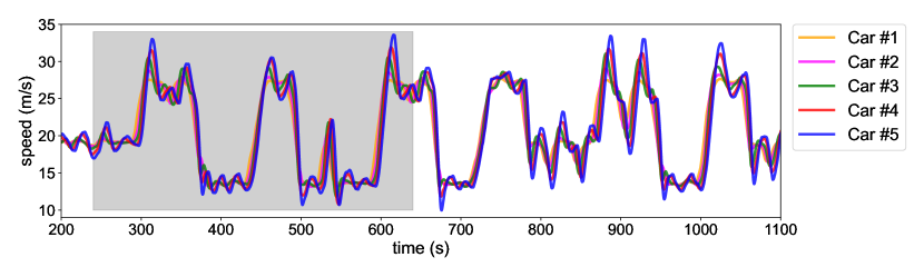
Figure 5: The illustration of $5$ vehicles’ speed profiles in the OpenACC dataset, where the shaded area ($240\sim 640$ s) is selected for the platoon simulation.

Since the HighD dataset only provides short trajectories with duration up to about $60$ s, we also evaluate our method on OpenACC trajectories with a duration of about $1000$ s. OpenACC dataset provides car-following records of a platoon, where a human driver operates the first vehicle, and four following vehicles in the platoon are autonomously controlled by an adaptive cruise control (ACC) module, as shown in Figure 5. The data in OpenACC is also downsampled to $5$ Hz.

Table 1: Posterior Mean of Model Parameters.

	$\bm{\theta}=[v_{0},s_{0},T,\alpha,\beta]$	$\sigma_{\eta}$	$\rho$
MA-IDM	$[17.173,3.642,1.129,0.536,1.982]$	$0.023$	($\sigma_{k}=0.193$, $\ell=1.32$ s)
Bayesian IDM ($p=0$)	$[21.090,3.724,0.946,0.518,1.542]$	$0.240$	$/$
Dynamic IDM ($p=1$)	$[29.600,3.233,1.183,0.771,4.144]$	$0.019$	$[0.994]$
Dynamic IDM ($p=2$)	$[26.651,3.367,1.193,0.753,3.534]$	$0.019$	$[1.241,-0.249]$
Dynamic IDM ($p=3$)	$[24.305,3.212,1.190,0.757,2.321]$	$0.017$	$[1.130,0.424,-0.570]$
Dynamic IDM ($p=4$)	$[25.648,3.222,1.168,0.711,2.417]$	$0.016$	$[0.920,0.581,-0.166,-0.361]$
Dynamic IDM ($p=5$)	$[23.968,3.241,1.200,0.749,2.742]$	$0.016$	$[0.919,0.572,-0.155,-0.334,-0.023]$
Dynamic IDM ($p=6$)	$[24.941,2.681,1.271,0.858,3.201]$	$0.016$	$[0.961,0.640,-0.150,-0.478,-0.215,0.236]$
Dynamic IDM ($p=7$)	$[25.881,2.479,1.280,0.836,3.132]$	$0.016$	$[0.903,0.702,-0.023,-0.446,-0.395,-0.023,0.278]$
Dynamic IDM ($p=8$)	$[25.930,2.493,1.274,0.797,3.308]$	$0.016$	$[0.842,0.710,0.061,-0.351,-0.392,-0.174,0.089,0.212]$
* Recommendation values (Treiber et al., 2000): $\bm{\theta}_{\text{rec}}=[33.3,2.0,1.6,1.5,1.67]$.

4.1.2 Model Training

We develop our model using PyMC 4.0 (Salvatier et al., 2016). We adopt the No-U-Turn Sampler, a kind of Hamiltonian Monte Carlo method (Hoffman et al., 2014), and set the burn-in steps as $3000$ to ensure the detailed balance condition holds for the Markov chains. We recommend and utilize the values $\bm{\theta}_{\text{rec}}=[33.3,2.0,1.6,1.5,1.67]$ in Treiber et al. (2000) for the IDM priors. In addition, we set $\lambda_{0}=100$ and $\lambda=2\times 10^{6}$ for the exponential distribution and $\eta=2$ for the LKJCholeskyCov distribution. Codes for all experimental results reported in this paper are released in https://github.com/Chengyuan-Zhang/IDM_Bayesian_Calibration.

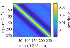
(a) The Empirical covariance matrix.

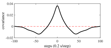
(b) The empirical covariance function.

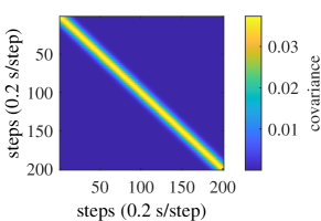
(c) The RBF kernel matrix.

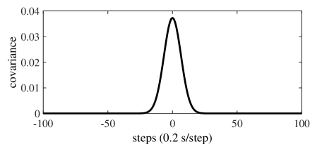
(d) The RBF kernel function.

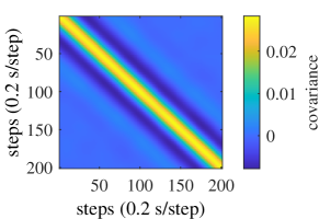
(e) The AR(4) covariance matrix.

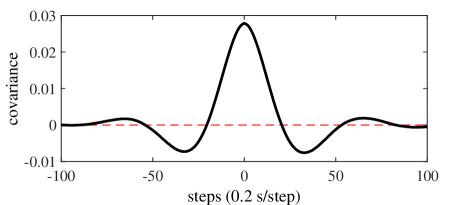
(f) The AR(4) covariance function.

Figure 6: The comparison among the empirical covariance, RBF kernel, and AR(4).

4.2 Calibration Results and Analysis

We compare the parameters of the Bayesian IDM with the dynamic IDM in Table 1. The parameter $\sigma_{\eta}$ represents the noise level of the i.i.d. errors, which decreases as the AR order increases. This indicates that the residual of the Bayesian IDM (when $p=0$) retains valuable information, as reflected by a higher value of $\sigma_{\eta}$. With higher AR order, more information is captured by the AR processes, reducing the contribution of the noise term. It is worth noting that the model with AR ($p=0$) is equivalent to the Bayesian IDM.

To compare the roles of GP and AR processes, we examine the RBF kernel matrix alongside the empirical covariance matrix estimated from real data and the covariance matrix generated from AR(4) (see Figure 6). The horizontal axes are time steps, where each time step represents $0.2$ s. The RBF kernel captures short-term positive correlations and fails to capture the long-term negative correlations observed in the residuals extracted from real driving data. To address this limitation, the dynamic IDM involves AR processes to capture both short-term positive and long-term negative correlations more realistically. This finding suggests that human drivers’ immediate stochastic component can be significantly impacted by their short-term $\epsilon_{d}^{(t)}$ values (up to $5$ s) (Zhang and Sun, 2022), potentially due to driving persistence (Treiber and Kesting, 2013b). Moreover, we uncover a notable observation: the stochastic components are also negatively correlated with the previous $\epsilon_{d}^{(t)}$ values in a long-term period ($5\sim 10$ s). For example, if the acceleration value of the human driver’s current action is greater than the expected behavior, i.e., the mean component in Equation 8, then in the following $5\sim 10$ s, the driver is very likely to take an action whose value is lower than the expected behaviors.

4.3 Simulations

One of the highlights of the dynamic IDM is its simulation scheme, leveraging the explicitly defined generative processes of the error term presented in Equation 8. This feature allows for the simulation and updating of future motions based on these generative processes. In what follows, we will introduce the parameter generation method for IDM and develop a stochastic simulator, which has been successfully tested in multiple cases.

4.3.1 Probabilistic Simulations

In Zhang and Sun (2022), the authors emphasize a key advantage of the Bayesian method over point estimator-based approaches. The Bayesian method provides joint distributions of parameters instead of only a single value. Consequently, instead of relying solely on the mean values from Table 1, we can draw a large number of samples from the posterior joint distributions to generate anthropomorphic IDM parameters effectively.

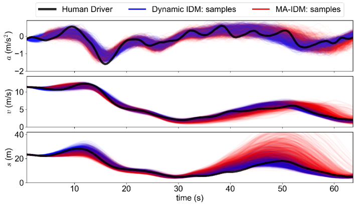
Figure 7: The probabilistic simulation results of a representative truck driver $\#211$. The black lines indicate the ground truth of human driving data; The red and blue lines are the predicted motion states with the parameter samples drawn from posteriors.

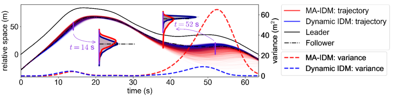
Figure 8: The time-space diagram of the follower’s posterior trajectories at the point view of another ‘observing’ vehicle with a constant mean speed.

Here We select one driver as an illustrative example to show the calibration results. We generate $N=1000$ sets of IDM parameters from the posteriors of the calibrated model. Then, given the leading vehicle’s full trajectories and the initial states of the follower, we simulate the follower’s full trajectories. The follower’s behavior is controlled by the calibrated IDM, with the addition of a random noise sampled from the generative processes. The simulation step is set as $0.2$ s. According to Equation 8, the simulation process involves three steps: (1) generating the mean model by sampling a set of IDM parameters from $\theta_{d}$, (2) computing the serial correlation term according to the historical information, and (3) sampling white noise randomly.

Table 2: Evaluations of the short-term (5 s) simulations with different models. All values are amplified by ten times to keep an efficient form.

= real values $\times 10$	$\mathrm{RMSE}(a)$	$\mathrm{RMSE}(v)$	$\mathrm{RMSE}(s)$	${\mathrm{CRPS}}(a)$	${\mathrm{CRPS}}(v)$	${\mathrm{CRPS}}(s)$
MA-IDM	$1.61\pm 0.83$	$2.72\pm 1.95$	$4.96\pm 3.44$	$0.82\pm 0.52$	$1.48\pm 1.21$	$3.05\pm 2.12$
Bayesian IDM ($p=0$)	$3.03\pm 0.51$	$2.88\pm 1.31$	$6.42\pm 3.88$	$1.10\pm 0.29$	$1.90\pm 1.00$	$4.19\pm 2.67$
Dynamic IDM ($p=1$)	$1.40\pm 0.51$	$2.35\pm 1.30$	$4.48\pm 2.72$	$0.98\pm 0.41$	$1.60\pm 0.97$	$2.80\pm 1.79$
Dynamic IDM ($p=2$)	$1.34\pm 0.53$	$2.33\pm 1.40$	$4.46\pm 2.81$	$0.88\pm 0.39$	$1.52\pm 0.99$	$2.64\pm 1.72$
Dynamic IDM ($p=3$)	$1.33\pm 0.58$	$2.30\pm 1.54$	$4.10\pm 2.89$	$0.74\pm 0.33$	$1.24\pm 0.93$	$2.00\pm 1.52$
Dynamic IDM ($p=4$)	$\mathbf{1.25\pm 0.56}$	$\mathbf{2.14\pm 1.46}$	$\mathbf{3.66\pm 2.69}$	${0.69\pm 0.33}$	$\mathbf{1.15\pm 0.91}$	${1.75\pm 0.14}$
Dynamic IDM ($p=5$)	${1.29\pm 0.62}$	${2.26\pm 1.47}$	${3.69\pm 2.54}$	${0.71\pm 0.36}$	${1.21\pm 0.87}$	$\mathbf{1.71\pm 1.29}$
Dynamic IDM ($p=6$)	$1.32\pm 0.61$	$2.44\pm 1.58$	${4.24\pm 2.95}$	$0.69\pm 0.31$	$1.27\pm 0.93$	${1.96\pm 1.51}$
Dynamic IDM ($p=7$)	$1.29\pm 0.61$	$2.39\pm 1.58$	$4.20\pm 2.89$	$\mathbf{0.62\pm 0.27}$	${1.19\pm 0.85}$	$1.89\pm 1.35$

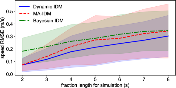
Figure 9: The performance comparison of simulations with fraction length varying from 2 seconds to 8 seconds.

We compare our model with the baseline MA-IDM (Zhang and Sun, 2022). Simulated trajectories are generated using parameter samples from $\bm{\theta}_{\#211}$ (Figure 7). In the comparison (Figure 8), our method shows tighter containment of ground truth within the envelope of posterior motion states, while MA-IDM requires a wider range. We evaluate the model performance using compare the absolute root mean square errors (RMSE) on motion states (acceleration, speed, and gap) between ground truth and fully simulated trajectories. Additionally, we use the continuously ranked probability score (CRPS) (Matheson and Winkler, 1976) to evaluate the performances of stochastic simulations and quantify the uncertainty of posterior motion states, which can be written as

$$\mathrm{CRPS}(y_{t})=\int_{-\infty}^{+\infty}\left(F(y)-\mathbbm{1}\{y>y_{t}\}\right)^{2}dy,$$ (15)

where $y_{t}$ is the observation at time $t$, $F$ is the forecast cumulative distribution function, and $\mathbbm{1}$ is the indicator function. We use RMSE/CRPS of many fraction samples with 5 s to evaluate the effectiveness of the short-term simulation, as shown in Table 2. Results indicate that our model outperforms Bayesian IDM and MA-IDM in 5-second simulations, especially with the AR order $p\geq 4$. In what follows, we mainly demonstrate the simulation performance using the model with AR(4). Recall that the length scale of the RBF kernel in MA-IDM is $\ell\approx 1.33$ s (Zhang and Sun, 2022), implying that MA-IDM generally performs well within 4 s (i.e., $3\ell$) simulations. To evaluate this, we also conducted simulations with fraction length varying from 2 s to 8 s, as shown in Figure 9, and the results indicate that the MA-IDM could perform reasonably well within 4 s. For those longer than $4$ s, the results of MA-IDM would then be more dominated by random noise rather than IDM, and its performance tend to be similar to the Bayesian IDM.

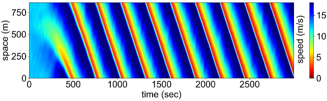
(a) Simulation with fixed IDM parameters and random white noise.

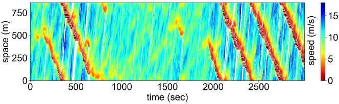
(b) Light traffic simulation with dynamic IDM ($p=4$).

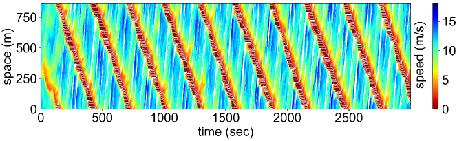
(c) Dense traffic simulation with dynamic IDM ($p=4$).

Figure 10: Time-space diagram of multi-vehicle car-following simulations. The parameters are sampled from the posteriors of (a) the hierarchical Bayesian IDM ($p=0$) and (b) the hierarchical dynamic IDM ($p=4$). (c) Simulation with dense traffic.

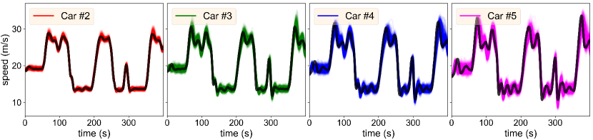
Figure 11: The multi-vehicle simulation in a platoon. Each vehicle’s initial state is set to be the same as it was at 240 seconds (refer to the shaded part in Figure 5) in the OpenACC dataset.

4.3.2 Multi-Vehicle Simulations: Ring-Road and Platoon

Long-term simulations enable the analysis of dynamic traffic behaviors at the macroscopic level by simultaneously simulating a group of vehicles. To validate the capability for large-scale traffic simulations, we conduct multi-vehicle simulation experiments in a ring-road scenario (Sugiyama et al., 2008) and a platoon.

Ring Road.

Key elements of the ring road include a ring radius of $128$ m, resulting in a circumference of approximately $804$ m, initial speeds set at $11.6$ m/s, $32$ vehicles for light traffic and $37$ vehicles for dense traffic simulated for $15000$ steps with simulation step as $0.2$ s. The multi-vehicle simulation is conducted with two different models, as shown in Figure 10. The top is simulated with Bayesian IDM and the others are simulated with the dynamic IDM ($p=4$). Figure 10 (a) presents a recurring pattern from the simulations with IDM parameters, although a stochastic term is introduced. On the contrary, different random car-following behaviors in the heterogeneous setting (see Figure 10 (b)) are obtained, indicating the drivers’ dynamic and diverse driving styles. Dynamic IDM simulation can produce various traffic phenomena in the real world, including shock wave dissipation.

Platoon.

In the platoon simulation, the first vehicle is the leader with its entire trajectory available. We simultaneously simulate four successive followers’ trajectories based on the dynamic IDM with AR(4). Figure 11 shows the four followers’ speed profiles, where the black lines represent the actual driving speed. We can see that the dynamic IDM still can accurately capture and replicate the real car-following behaviors even in long-range simulations.

5 Conclusion

This paper presents a dynamic regression framework for calibrating and simulating car-following models, which plays a critical role in understanding traffic flow dynamics. Our approach addresses a key limitation of existing car-following models by incorporating historical information, resulting in a more accurate reproduction of real-world driving behavior. By integrating AR processes into the error modeling, we offer a statistically rigorous alternative to the assumption of independent errors commonly found in current models. This enables the consideration of higher-order historical information, leading to improved simulation and prediction accuracy. Experiment results indicate that modeling human car-following behavior should incorporate actions from the past 10 s, capturing short-term positive correlations ($0\sim 5$ s) and long-term negative correlations ($5\sim 10$ s) in real driving data. The framework’s effectiveness is demonstrated through its application to the HighD data. The proposed framework inherits the parsimonious feature of traditional car-following models and provides more realistic simulations. In conclusion, our research sheds light on a potential direction for the development of high-fidelity microscopic traffic simulation models. By integrating historical data, our dynamic regression framework enables more accurate predictions and simulations of car-following behavior, which is crucial for traffic management and planning. We hope our findings could stimulate further research in this direction, fostering a deep understanding of traffic flow dynamics and the development of advanced and efficient microscopic traffic models.

However, as with all research, there are avenues for further development. Future work could explore incorporating a mean model as a car-following model with time-varying parameters to enhance adaptability to diverse scenarios and driving modes. Additionally, adding a moving average component might capture the temporal dependence and irregular patterns, and reduce the noise level through smoothing.

Acknowledgments

C. Zhang would like to thank the McGill Engineering Doctoral Awards (MEDA), the Interuniversity Research Centre on Enterprise Networks, Logistics and Transportation (CIRRELT), Fonds de recherche du Québec – Nature et technologies (FRQNT), and the Natural Sciences and Engineering Research Council (NSERC) of Canada for providing scholarships and funding to support this study.

Appendix

(1) Calibration on speed data with observation noise

Recall that our model follows

$$a^{(t)}= \,\mathrm{IDM}^{(t)}+\epsilon^{(t)},$$

$$\epsilon^{(t)}= \,\rho_{1}\epsilon^{(t-1)}+\rho_{2}\epsilon^{(t-2)}+\dots+\rho_{p}\epsilon^{(t-p)}+\eta,$$

$$\eta\,\stackon{$\sim$}{\tiny{\textit{i.i.d.}}}\, \mathcal{N}(0,\sigma^{2}_{\eta}),$$

and given the dynamic updating in Equation 3a ${v}^{(t+1)}=v^{(t)}+a^{(t)}\Delta t$, then we have

$$a^{(t)}= \,\mathrm{IDM}^{(t)}+\rho_{1}\left(a^{(t-1)}-\mathrm{IDM}^{(t-1)}\right)+\rho_{2}\left(a^{(t-2)}-\mathrm{IDM}^{(t-2)}\right)$$

$$\,+\cdots+\rho_{p}\left(a^{(t-p)}-\mathrm{IDM}^{(t-p)}\right)+\eta,$$ (16a)

$$v^{(t+1)}= \,v^{(t)}+\mathrm{IDM}^{(t)}\Delta t+\rho_{1}\left(a^{(t-1)}\Delta t-\mathrm{IDM}^{(t-1)}\Delta t\right)+\cdots$$

$$\,+\rho_{p}\left(a^{(t-p)}\Delta t-\mathrm{IDM}^{(t-p)}\Delta t\right)+\eta\Delta t$$ (16b)

$$= \,v^{(t)}+\mathrm{IDM}^{(t)}\Delta t+\rho_{1}\left((v^{(t-1)}+a^{(t-1)}\Delta t)-(v^{(t-1)}+\mathrm{IDM}^{(t-1)}\Delta t)\right)+\cdots$$

$$\,+\rho_{p}\left((v^{(t-p)}+a^{(t-p)}\Delta t)-(v^{(t-p)}+\mathrm{IDM}^{(t-p)}\Delta t)\right)+\eta\Delta t$$ (16c)

$$= \,v^{(t)}+\mathrm{IDM}^{(t)}\Delta t+\rho_{1}\left(v^{(t)}-(v^{(t-1)}+\mathrm{IDM}^{(t-1)}\Delta t)\right)+\cdots$$

$$\,+\rho_{p}\left(v^{(t-(p-1))}-(v^{(t-p)}+\mathrm{IDM}^{(t-p)}\Delta t)\right)+\eta\Delta t$$ (16d)

$$= \,v^{(t)}+\mathrm{IDM}^{(t)}\Delta t+\sum_{k=1}^{p}\rho_{k}\left(v^{(t-(k-1))}-v^{(t-k)}\right)-\sum_{k=1}^{p}\rho_{k}\mathrm{IDM}^{(t-k)}\Delta t+\eta\Delta t.$$ (16e)

Such that we can give the likelihood of a noisy observation as

$$\hat{v}^{(t+1)}\sim\mathcal{N}\left(\bar{v}^{(t+1)},(\sigma_{\eta}\Delta t)^{2}+\sigma_{v}^{2}\right),$$ (17)

where $\bar{v}^{(t+1)}=v^{(t)}+\mathrm{IDM}^{(t)}\Delta t+\sum_{k=1}^{p}\rho_{k}\left(v^{(t-(k-1))}-v^{(t-k)}\right)-\sum_{k=1}^{p}\rho_{k}\mathrm{IDM}^{(t-k)}\Delta t$, $\hat{v}^{(t+1)}$ is the observed data of the true speed ${v}^{(t+1)}$, and $\sigma_{v}^{2}$ is the variance of the observation noise.

(2) Calibration on position/spacing data with observation noise

Similar to the previous approach, from Equation 3b we have $x^{(t+1)}=x^{(t)}+v^{(t)}\Delta t+\frac{1}{2}a^{(t)}\Delta t^{2}$; then according to Equation 16e, we can reformat $x^{(t+1)}$ as

$$x^{(t+1)}= \,x^{(t)}+\frac{1}{2}v^{(t)}\Delta t+\frac{1}{2}\biggl{(}v^{(t)}+\mathrm{IDM}^{(t)}\Delta t+\sum_{k=1}^{p}\rho_{k}\left(v^{(t-(k-1))}-v^{(t-k)}\right)$$ (18a)

$$-\sum_{k=1}^{p}\rho_{k}\mathrm{IDM}^{(t-k)}\Delta t+\eta\Delta t\biggr{)}\Delta t$$

$$= \,x^{(t)}+v^{(t)}\Delta t+\frac{1}{2}\mathrm{IDM}^{(t)}\Delta t^{2}+\frac{1}{2}\sum_{k=1}^{p}\rho_{k}\left(v^{(t-(k-1))}-v^{(t-k)}\right)\Delta t$$ (18b)

$$-\frac{1}{2}\sum_{k=1}^{p}\rho_{k}\mathrm{IDM}^{(t-k)}\Delta t^{2}+\frac{1}{2}\eta\Delta t^{2}.$$

Accordingly, the likelihood is written as

$$\hat{x}^{(t+1)}\sim\mathcal{N}\left(\bar{x}^{(t+1)},\Bigl{(}\frac{1}{2}\sigma_{\eta}\Delta t^{2}\Bigr{)}^{2}+\sigma_{x}^{2}\right),$$ (19)

where the mean $\bar{x}^{(t+1)}=x^{(t)}+v^{(t)}\Delta t+\frac{1}{2}\mathrm{IDM}^{(t)}\Delta t^{2}+\frac{1}{2}\sum_{k=1}^{p}\rho_{k}\left(v^{(t-(k-1))}-v^{(t-k)}\right)\Delta t-\frac{1}{2}\sum_{k=1}^{p}\rho_{k}\mathrm{IDM}^{(t-k)}\Delta t^{2}$, $\hat{x}^{(t+1)}$ is the observed data of the true position ${x}^{(t+1)}$, and $\sigma_{x}^{2}$ is the variance of the observation noise of position data. Note that this is a position-based form, but one can easily adapt it into a gap-based form.

References

- Bando et al. (1995) Masako Bando, Katsuya Hasebe, Akihiro Nakayama, Akihiro Shibata, and Yuki Sugiyama. Dynamical model of traffic congestion and numerical simulation. Physical review E, 51(2):1035, 1995.
- Bhattacharyya et al. (2020) Raunak P Bhattacharyya, Ransalu Senanayake, Kyle Brown, and Mykel J Kochenderfer. Online parameter estimation for human driver behavior prediction. In 2020 American Control Conference (ACC), pages 301–306. IEEE, 2020.
- Derbel et al. (2012) Oussama Derbel, Tamás Péter, Hossni Zebiri, Benjamin Mourllion, and Michel Basset. Modified intelligent driver model. Periodica Polytechnica. Transportation Engineering, 40(2):53, 2012.
- Gipps (1981) Peter G Gipps. A behavioural car-following model for computer simulation. Transportation Research Part B: Methodological, 15(2):105–111, 1981.
- He et al. (2015) Zhengbing He, Liang Zheng, and Wei Guan. A simple nonparametric car-following model driven by field data. Transportation Research Part B: Methodological, 80:185–201, 2015.
- Hoffman et al. (2014) Matthew D Hoffman, Andrew Gelman, et al. The no-u-turn sampler: adaptively setting path lengths in hamiltonian monte carlo. J. Mach. Learn. Res., 15(1):1593–1623, 2014.
- Hoogendoorn and Hoogendoorn (2010) Serge Hoogendoorn and Raymond Hoogendoorn. Calibration of microscopic traffic-flow models using multiple data sources. Philosophical Transactions of the Royal Society A: Mathematical, Physical and Engineering Sciences, 368(1928):4497–4517, 2010.
- Krajewski et al. (2018) Robert Krajewski, Julian Bock, Laurent Kloeker, and Lutz Eckstein. The highd dataset: A drone dataset of naturalistic vehicle trajectories on german highways for validation of highly automated driving systems. In 2018 21st International Conference on Intelligent Transportation Systems (ITSC), pages 2118–2125, 2018.
- Lefèvre et al. (2014) Stéphanie Lefèvre, Chao Sun, Ruzena Bajcsy, and Christian Laugier. Comparison of parametric and non-parametric approaches for vehicle speed prediction. In 2014 American Control Conference, pages 3494–3499. IEEE, 2014.
- Lewandowski et al. (2009) Daniel Lewandowski, Dorota Kurowicka, and Harry Joe. Generating random correlation matrices based on vines and extended onion method. Journal of multivariate analysis, 100(9):1989–2001, 2009.
- Ma and Andréasson (2005) Xiaoliang Ma and Ingmar Andréasson. Dynamic car following data collection and noise cancellation based on the kalman smoothing. In IEEE International Conference on Vehicular Electronics and Safety, 2005., pages 35–41. IEEE, 2005.
- Matheson and Winkler (1976) James E Matheson and Robert L Winkler. Scoring rules for continuous probability distributions. Management science, 22(10):1087–1096, 1976.
- Montanino and Punzo (2015) Marcello Montanino and Vincenzo Punzo. Trajectory data reconstruction and simulation-based validation against macroscopic traffic patterns. Transportation Research Part B: Methodological, 80:82–106, 2015.
- Ossen et al. (2006) Saskia Ossen, Serge P Hoogendoorn, and Ben GH Gorte. Interdriver differences in car-following: A vehicle trajectory–based study. Transportation Research Record, 1965(1):121–129, 2006.
- Punzo et al. (2011) Vincenzo Punzo, Maria Teresa Borzacchiello, and Biagio Ciuffo. On the assessment of vehicle trajectory data accuracy and application to the next generation simulation (ngsim) program data. Transportation Research Part C: Emerging Technologies, 19(6):1243–1262, 2011.
- Punzo et al. (2012) Vincenzo Punzo, Biagio Ciuffo, and Marcello Montanino. Can results of car-following model calibration based on trajectory data be trusted? Transportation research record, 2315(1):11–24, 2012.
- Punzo et al. (2014) Vincenzo Punzo, Marcello Montanino, and Biagio Ciuffo. Do we really need to calibrate all the parameters? variance-based sensitivity analysis to simplify microscopic traffic flow models. IEEE Transactions on Intelligent Transportation Systems, 16(1):184–193, 2014.
- Punzo et al. (2021) Vincenzo Punzo, Zuduo Zheng, and Marcello Montanino. About calibration of car-following dynamics of automated and human-driven vehicles: Methodology, guidelines and codes. Transportation Research Part C: Emerging Technologies, 128:103165, 2021.
- Saifuzzaman and Zheng (2014) Mohammad Saifuzzaman and Zuduo Zheng. Incorporating human-factors in car-following models: a review of recent developments and research needs. Transportation research part C: emerging technologies, 48:379–403, 2014.
- Salvatier et al. (2016) John Salvatier, Thomas V Wiecki, and Christopher Fonnesbeck. Probabilistic programming in python using pymc3. PeerJ Computer Science, 2:e55, 2016.
- Sugiyama et al. (2008) Yuki Sugiyama, Minoru Fukui, Macoto Kikuchi, Katsuya Hasebe, Akihiro Nakayama, Katsuhiro Nishinari, Shin-ichi Tadaki, and Satoshi Yukawa. Traffic jams without bottlenecks—experimental evidence for the physical mechanism of the formation of a jam. New journal of physics, 10(3):033001, 2008.
- Sun et al. (2022) Chao Sun, Jianghao Leng, and Fengchun Sun. A fast optimal speed planning system in arterial roads for intelligent and connected vehicles. IEEE Internet of Things Journal, 9(20):20295–20307, 2022.
- Taylor et al. (2015) Jeffrey Taylor, Xuesong Zhou, Nagui M Rouphail, and Richard J Porter. Method for investigating intradriver heterogeneity using vehicle trajectory data: A dynamic time warping approach. Transportation Research Part B: Methodological, 73:59–80, 2015.
- Treiber and Helbing (2003) Martin Treiber and Dirk Helbing. Memory effects in microscopic traffic models and wide scattering in flow-density data. Physical Review E, 68(4):046119, 2003.
- Treiber and Kesting (2013a) Martin Treiber and Arne Kesting. Microscopic calibration and validation of car-following models–a systematic approach. Procedia-Social and Behavioral Sciences, 80:922–939, 2013a.
- Treiber and Kesting (2013b) Martin Treiber and Arne Kesting. Traffic flow dynamics. Traffic Flow Dynamics: Data, Models and Simulation, Springer-Verlag Berlin Heidelberg, pages 983–1000, 2013b.
- Treiber and Kesting (2017) Martin Treiber and Arne Kesting. The intelligent driver model with stochasticity-new insights into traffic flow oscillations. Transportation research procedia, 23:174–187, 2017.
- Treiber et al. (2000) Martin Treiber, Ansgar Hennecke, and Dirk Helbing. Congested traffic states in empirical observations and microscopic simulations. Physical review E, 62(2):1805, 2000.
- Treiber et al. (2010) Martin Treiber, Arne Kesting, and Dirk Helbing. Three-phase traffic theory and two-phase models with a fundamental diagram in the light of empirical stylized facts. Transportation Research Part B: Methodological, 44(8-9):983–1000, 2010.
- Wang et al. (2018) Wenshuo Wang, Junqiang Xi, and Ding Zhao. Learning and inferring a driver’s braking action in car-following scenarios. IEEE Transactions on Vehicular Technology, 67(5):3887–3899, 2018.
- Wang et al. (2017) Xiao Wang, Rui Jiang, Li Li, Yilun Lin, Xinhu Zheng, and Fei-Yue Wang. Capturing car-following behaviors by deep learning. IEEE Transactions on Intelligent Transportation Systems, 19(3):910–920, 2017.
- Zhang and Sun (2022) Chengyuan Zhang and Lijun Sun. Bayesian calibration of the intelligent driver model. arXiv preprint arXiv:2210.03571, 2022.
- Zhang et al. (2021) Chengyuan Zhang, Jiacheng Zhu, Wenshuo Wang, and Junqiang Xi. Spatiotemporal learning of multivehicle interaction patterns in lane-change scenarios. IEEE Transactions on Intelligent Transportation Systems, 2021.
- Zhang et al. (2022) Yifan Zhang, Xinhong Chen, Jianping Wang, Zuduo Zheng, and Kui Wu. A generative car-following model conditioned on driving styles. Transportation research part C: emerging technologies, 145:103926, 2022.
- Zhou et al. (2023) Shirui Zhou, Shiteng Zheng, Martin Treiber, Junfang Tian, and Rui Jiang. On the calibration of stochastic car following models. arXiv preprint arXiv:2302.04648, 2023.