Eötvös Loránd University
Faculty of Science
Institute of Physics and Astronomy

Munkhjargal LKHAGVADORJ

Supervisor:	Gábor FACSKÓ, PhD
	Department of Space Physics and Space Technology
	Wigner Research Centre for Physics
Co-supervisor:	Krisztina Éva GABÁNYI, PhD
	Department of Astronomy, Eötvös Loránd University

Budapest, May 30, 2023

Abstract

Interplanetary shocks are one of the crucial dynamic processes in the Heliosphere. They accelerate particles into a high energy, generate plasma waves, and could potentially trigger geomagnetic storms in the terrestrial magnetosphere disturbing significantly our technological infrastructures. In this study, two IP shock events are selected to study the temporal variations of the shock parameters using magnetometer and ion plasma measurements of the STEREO$-$A and B, the Wind, Cluster fleet, and the ACE spacecraft. The shock normal vectors are determined using the minimum variance analysis (MVA) and the magnetic coplanarity methods (CP). During the May 07 event, the shock parameters and the shock normal direction are consistent. The shock surface appears to be tilted almost the same degree as the Parker spiral, and the driver could be a CIR. During the April 23 event, the shock parameters do not change significantly except for the shock $\theta_{Bn}$ angle, however, the shape of the IP shock appears to be twisted along the transverse direction to the Sun-Earth line as well. The driver of this rippled shock is SIRs/CIRs as well. Being a fast-reverse shock caused this irregularity in shape.

Keywords: Interplanetary shock, Solar wind, Space plasma, Heliosphere, Co-rotating interaction region, Stream interaction region, Coronal mass ejection.

Chapter 1 Introduction

The solar corona is hotter than the photosphere, the chromosphere, and the transient layers beneath it. As a result, the high temperatures ionize atoms, creating a plasma of free-moving electrons and ions, known as the solar wind. Historically, (Parker, 1958) predicted the existence of the solar wind and coined the term ”solar wind”. He deducted it based on German astronomer Ludwig Bierman’s observation of how the comet tail always points away from the Sun (Biermann, 2013). The existence of the solar wind was confirmed by the Mariner 2 spacecraft (Snyder and Neugebauer, 1965). The solar wind is a collisionless plasma, and it flows at both supersonic and super-Alfvénic speed, meaning they exceed the Alfvén speed, which is the speed of magnetohydrodynamic waves in a plasma. A shock wave is where a fluid changes from supersonic to subsonic speed. Therefore, the fast-moving solar wind tends to create a shock on its journey. Hence, interplanetary (IP) shocks are common through the heliosphere, which is a bubble-like region of space surrounding the Sun and extending far beyond the orbits of the planets and is filled with the solar wind. There are a few varieties of shocks such as planetary bow shocks, shocks that are risen due to the stream interaction regions (SIR), which is called co-rotation interaction region (CIR) when extending beyond 1 AU, and coronal mass ejection (CME) driven shocks. IP shocks are one of the main and efficient accelerators of energetic particles (Tsurutani and Lin, 1985; Keith and Heikkila, 2021). These accelerated particles can cause disturbances to the geomagnetic field and are hazardous to astronauts and satellites. (IP) shocks driven by (CMEs) precede large geomagnetic storms (Gonzalez et al., 1994). Large geomagnetic storms can damage oil and gas pipelines and interfere with electrical power infrastructures. GPS navigation and high-frequency radio communications are also affected by ionosphere changes brought on by geomagnetic storms (Cid et al., 2014) and can cause internet disruptions around the world for many months (Jyothi, 2021). Therefore, IP shocks are important in determining and understanding space weather.

The main goal of this thesis is to study and determine parameters such as IP shock normals, upstream and downstream plasma parameters (magnetic field, density, temperature, velocity), and how they vary in their temporal evolution. There are several methods for determining the shock normal vector (Paschmann and Daly, 1998). In this thesis, the minimum variance analysis (MVA) and the magnetic coplanarity method (CP) are used. These two methods are primarily utilized because they require solely magnetic field data. The data are from NASA’s twin Solar Terrestrial Relations Observatory Ahead (STEREO$-$A) and Behind (STEREO$-$B) (Kaiser et al., 2008), the Wind (Ogilvie and Desch, 1997), and Advanced Composition Explorer (ACE) spacecraft Stone et al. (1998c), and ESA’s four identical Cluster constellation satellites–Cluster-1 (C1), Cluster-2 (C1), Cluster-3 (C3), and Cluster-4 (C4) (Escoubet et al., 1997). The temporal resolution of the magnetometers of the heliospheric (and the Cluster) spacecraft is significantly higher than the plasma instruments because the variations are quite slow in the heliosphere. So, any agreement between the two methods indicates relatively accurate shock normal vectors (Facskó et al., 2008, 2009, 2010). Here, two events are studied, one is May 07, 2007, and the other is April 23. The data selection year, 2007, is special because location wise it was the year when twin STEREO$-$A and B spacecraft were closer to the Sun-Earth line until their gradual separation from each other in the following years. Later, the spatial separation is so high that it is hard to distinguish the spatial and temporal changes. Hence, shocks during this period are proper to study shock propagation and their temporal developments in the case of using these spacecraft. Chapter 2 introduces the basics of plasma physics and magnetohydrodynamics, which are the governing equations of these heliosphere phenomena. Chapter 3 discusses a brief description of the Sun, the solar wind, and the interplanetary magnetic field. Chapter 4 is about instrumentation, database, and methods. Chapter 5 presents the results and discusses them. Chapter 6 is the summary and conclusions.

Chapter 2 Basics of Magnetohydrodynamics

2.1 Plasma

The term plasma for this state of matter was coined by Irvin Langmuir after its similarity with the blood plasma carrying white and red cells (Tonks, 1967). A plasma is a set of charged particles made up of an equal number of free carriers for positive and negative charges. Having nearly the same number of opposite charges ensures that the plasma appears quasi-neutral from the outside. Free particle carriers mean the particles inside a plasma must have enough kinetic (thermal) energy to overcome the potential energies of their nearest neighbors, which means a plasma is a hot and ionized gas. There are the three basic criteria for a plasma (Baumjohann and Treumann, 2012; Chapters 1-4).
The first criterion is a test-charged particle is clouded by its opposite-charged particles, canceling the electric field of the test particle. This is known as the Debye shielding and its so$-$called Debye$-$lenght, $\lambda_{D}$, is defined as follows:

$$\lambda_{D}=\sqrt{\frac{\epsilon_{0}k_{B}T_{e}}{n_{e}e^{2}}},$$ (2.1)

where $\epsilon_{0}$ is the free space permittivity, $k_{B}$ the Boltzmann constant, $T_{e}=T_{i}$ the electron and ion temperature, $n_{e}$ the electron plasma density, and $e$ electric charge. To ensure the quasineutrality of a plasma, the system length $L$ must be greater than the Debye length

$$L>>\lambda_{D}$$ (2.2)

The second criterion is since the Debye shielding results from the collective behavior of particles inside the Debye sphere with the radius $\lambda_{D}$, the Debye sphere must contain enough particles

$$\Lambda=n_{e}\lambda^{3}_{D}>>1$$ (2.3)

which indicates the mean potential energy of particles between their nearest neighbors must be less than their mean individual energies.
The third criterion is the collision time scale $\tau$ of the system is greater than the inverse of the plasma $\omega_{p}^{-1}$, electron $\Omega_{e}^{-1}$, and ion $\Omega_{i}^{-1}$ cyclotron gyrofrequencies.

$$\tau>>\omega_{p}^{-1},\Omega_{i}^{-1},\Omega_{e}^{-1}$$ (2.4)

By solving each particle, plasma dynamics can be described, but this approach is too difficult and inefficient. Therefore, there are certain approximations, depending on the corresponding problems. Magnetohydrodynamics is one such approximation that instead of taking account of individual particles, the plasma is assumed as a magnetized fluid.

2.2 The single fluid MHD

In this section, the magnetohydrodynamics (MHD) equations are briefly introduced without too much detail and derivations. The following formulizations are based on (Baumjohann and Treumann, 2012)[page 138-158], (Murphy, 2014), (Freidberg, 2014) and (Antonsen Jr., 2019). Magnetohydrodynamics (MHD) was developed by Hannes Alfvén (Davidson, 2002). MHD equations are the result of coupling the Navier-Stokes equations (the fluid equations) to the Maxwell equations. In the MHD, the plasma is treated as a single fluid with macroscopic parameters such as average density, temperature, and velocity. Since plasma consists of generally two species of particles, namely electrons, and ions, the different species should be handled together. Hence, the single fluid approximation is utilized. The single fluid variables are defined as follows:
Mass density, considering the mass $m_{e}$ of an electron is significantly lower than the mass $m_{i}$ of an ion, $m_{e}<<m_{i}$:

$$\rho_{m}=n_{e}m_{e}+n_{i}m_{i}\approx m_{i}n$$ (2.5)

Momentum density:

$$\rho_{m}\mathbf{v}=n_{e}m_{e}\mathbf{u_{e}}+n_{i}m_{i}\mathbf{u_{i}}\approx\rho_{m}\mathbf{u_{i}}$$ (2.6)

where $\mathbf{v}$, $\mathbf{u_{e}}$, $\mathbf{u_{i}}$ are plasma, electron, ion velocities respectively, and $\rho$ is the plasma density, $n_{e}$, $n_{i}$ are the electron and ion number densities.

Current density:

$$\mathbf{J}=n_{e}q_{e}\mathbf{u}_{e}+n_{i}q_{i}\mathbf{u}_{i}=en(\mathbf{u}_{i}-\mathbf{u}_{e})$$ (2.7)

where $q_{e}$ and $q_{i}$ are electron and ion charges.

Total pressure:

$$\mathbf{P}=\mathbf{P}_{e}+\mathbf{P}_{i}$$ (2.8)

By using the single fluid variables, the single fluid MHD equations can be defined as follows:
The continuity equation for the mass density:

$$\frac{\partial\rho_{m}}{\partial t}+\nabla\cdot(\rho_{m}\vec{v})=0$$ (2.9)

The momentum equation:

$$\frac{\partial(\rho_{m}\mathbf{v})}{\partial t}+\nabla\cdot(\rho_{m}\mathbf{v}\mathbf{v})=-\nabla\cdot\mathbf{P}+\rho_{e}\mathbf{E}+\mathbf{J}\crossproduct\mathbf{B}$$ (2.10)

where $\rho_{e}$ denotes the charge density, and $\mathbf{E}$, $\mathbf{B}$ electric and magnetic fields.
The generalized Ohm’s law:

$$\mathbf{E}+\mathbf{v}\crossproduct\mathbf{B}=\eta\mathbf{J}+\frac{1}{ne}\mathbf{J}\crossproduct\mathbf{B}-\frac{1}{ne}\nabla\cdot\mathbf{P}_{e}+\frac{m_{e}}{ne^{2}}\frac{\partial\mathbf{j}}{\partial t},$$ (2.11)

where $\eta$ is magnetic diffusivity , and $\eta\mathbf{J}$ is the resistive term.
Ampère’s law:

$$\nabla\crossproduct\mathbf{B}=\mu_{0}\mathbf{J}+\mu_{0}\epsilon_{0}\frac{\partial\mathbf{E}}{\partial t}$$ (2.12)

where $\mu_{0}$ is the vacuum magnetic permeability, $\epsilon_{0}$ is vacuum permittivity

Faraday’s law:

$$\nabla\crossproduct\mathbf{E}=-\frac{\partial\mathbf{B}}{\partial t}$$ (2.13)

And finally, the magnetic field divergence constraint:

$$\nabla\cdot\mathbf{B}=0$$ (2.14)

The MHD approximations are valid when the characteristic speed of the system is much slower than the speed of light,

$$\mathbf{v}<<c$$ (2.15)

the characteristic frequency, $\omega$, must be smaller than the ion cyclotron frequency $\omega_{i}$

$$\omega<<\omega_{i}$$ (2.16)

the characteristic scale length $L$ of the system must be longer than the mean free path $r_{gi}$ of ion gyroradius

$$L>r_{gi}$$ (2.17)

the characteristic scale times must be larger than the collision times as stated in equation 2.4.

2.3 MHD wave modes

Plasma is considered a highly conductive fluid, which consists of charged particles. Therefore, MHD waves in plasma fundamentally arise from two distinct wave speeds: the sound speed of a fluid and the Alfvén speed, which is due to the magnetic field pressure and tension. Their combination gives rise to magnetosonic waves. Thus, in MHD there are three wave modes–namely slow magnetosonic, the shear-Alfvénic and the fast magnetosonic waves (Fitzpatrick, 2014) in addition to the sound wave, as seen in Figure 2.1.

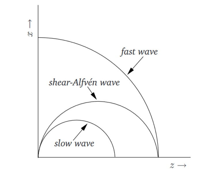
Figure 2.1: Phase velocities of the three MHD waves. (Figure is from Fitzpatrick, 2014; Figure 7.1)

The derivation of the waves can be obtained from the linearized MHD dispersion relation.
The sound wave is due to a compressible fluid and the wave is longitudinal. The sound speed is defined as:

$$C_{s}=\sqrt{\frac{\gamma k_{B}T}{m_{i}}}$$ (2.18)

where $\gamma$ is the polytropic index and in space plasma, it is in the range $1<\gamma<5/3$ (Livadiotis and Nicolaou, 2021), $k_{B}$ is the Boltzmann constant, $T$ is temperature, $m_{i}$ is mass of a particle species. The Mach number, a ratio of flow to the (thermal) sound speed

$$M_{s}=\sqrt{\frac{m_{i}v^{2}}{\gamma k_{B}T}}$$ (2.19)

The shear Alfvénic wave is incompressible and transverse. The Alfvén speed is defined as follows:

$$V_{A}=\sqrt{\frac{B^{2}}{\mu_{0}\rho}}$$ (2.20)

here $\frac{B^{2}}{\mu_{0}}$ is the magnetic pressure and $\rho$ is density.
Similarly, the magnetic Mach number, which is defined as a ratio between the flow speed $V_{flow}$ and the Alfvénic speed $V_{A}$, is defined as follows:

$$M_{A}=\frac{V_{flow}}{V_{A}}$$ (2.21)

The magnetosonic waves are as follows:

$$C^{2}_{ms}=\frac{1}{2}(C^{2}_{s}+V^{2}_{A})\bigg{[}1\pm\bigg{(}1-4\frac{cos^{2}\theta}{b^{2}}\bigg{)}\bigg{]},$$ (2.22)

where $b$ term is as follows:

$$b=\frac{C_{s}}{V_{A}}+\frac{V_{A}}{C_{s}}\geq 2$$ (2.23)

The equation 2.22 has two terms. The term containing (+) is the fast magnetosonic wave while the one containing (-) is the slow magnetosonic wave.
When $V_{A}>>V_{s}$ or $V_{s}>>V_{A}$ in 2.23, as well as the wave propagation direction, is nearly perpendicular to the magnetic field $(cos^{2}\theta<<1)$, the slow magnetosonic wave speed becomes as follows:

$$C^{2}_{ms}=cos^{2}\theta\frac{C_{s}^{2}V_{A}^{2}}{(c^{2}_{s}+V^{2}_{A})}$$ (2.24)

while the fast magnetosonic wave is simplified as follows:

$$C_{ms}=\sqrt{C_{s}^{2}+V_{A}^{2}}$$ (2.25)

from 2.25, the fast magnetosonic Mach number is defined as

$$M_{ms}=\frac{V_{flow}}{C_{ms}}$$ (2.26)

2.4 MHD discontinuities

When plasmas of different properties collide, they reach equilibria, resulting in the boundaries separating neighboring plasma regions (Baumjohann and Treumann, 2012; Chapter 8). These boundary regions are called discontinuities, and in astrophysics, heliopause and magnetopause are examples of these discontinuities. Through discontinuities, the field and plasma parameters change abruptly, but these sudden changes satisfy a few conditions, namely the Rankine-Hugoniot jump conditions. To derive the jump conditions, it is suitable to integrate the conservation laws across the discontinuity. Therefore, it is better to write the single fluid MHD equations 2.2 in conservative form, assuming that the two sides of the discontinuity satisfy an ideal single-fluid MHD. Following some notations and derivations of (Baumjohann and Treumann, 2012; Chapter 8), the ideal single-fluid MHD equations in conservative forms are defined below:

$$\frac{\partial(\rho\mathbf{v})}{\partial t}+\nabla\cdot\Bigg{[}(\rho\mathbf{vv})+\left(\mathbf{P}+\frac{B^{2}}{2\mu_{0}}\mathbf{I}\right)-\frac{1}{\mu_{0}}(\mathbf{BB})\Bigg{]}=0,$$ (2.27)

where $\mathbf{P}$ the plasma pressure, B the magnetic field magnitude,$\mathbf{B}$ the magnetic field vector, $\mu_{0}$ the vacuum permeability, and $\mathbf{I}$ the identity tensor.
The induction equation:

$$\frac{\partial\mathbf{B}}{\partial t}=\nabla\crossproduct(\mathbf{v}\crossproduct\mathbf{B})$$ (2.28)

The divergence of the magnetic field:

$$\nabla\cdot\mathbf{B}=0$$ (2.29)

The energy conservation equation:

$$\nabla\cdot\Bigg{\{}\rho\mathbf{v}\left[\frac{1}{2}v^{2}+w+\frac{1}{\rho}\left(p+\frac{B^{2}}{\mu_{0}}\right)\right]-\frac{1}{\mu_{0}}(\mathbf{v}\cdot\mathbf{B})\mathbf{B}\Bigg{\}}=0,$$ (2.30)

where for slowly variable fields $\mu_{0}j=\nabla\crossproduct\mathbf{B}$ and the ideal Ohm’s law $E=-\nabla\crossproduct\mathbf{B}$ are implemented as well as neglecting charges $\rho\mathbf{E}=0$, and $w=\frac{c_{v}P}{\rho k_{B}}$ is the internal enthalpy.
For completion, the equation of state is set:

$$\mathbf{P}=p\mathbf{I},$$ (2.31)

where $p$ is the scalar pressure. Choosing a co-moving reference frame with discontinuity, a steady-state situation is assumed that all the time-dependent terms are canceled, leaving the flux terms in the conservation laws. A discontinuity causes the plasma parallel to the discontinuity to stay the same while the plasma perpendicular to the discontinuity changes. For these reasons, a two-dimensional function S(x)=0 can be used to characterize the discontinuity surface, and the normal vector to the discontinuity, $\mathbf{n}$, is defined as follows

$$\mathbf{n}=-\frac{\nabla S}{|\nabla S|}$$ (2.32)

To the direction of the $\mathbf{n}$ the vector derivative has only one component $\nabla=\mathbf{n}(\frac{\partial}{\partial n})$. After these considerations, integrating over the discontinuity for the flux terms has to be done. Remembering only two perpendicular sides of the discontinuity contribute twice to the integration, a quantity X crossing $S$ becomes

$$\oint_{s}\frac{\partial X}{\partial n}dn=2\int_{1}^{2}\frac{\partial X}{\partial n}dn=2(X_{2}-X_{1})=2[X],$$ (2.33)

where parenthesis $[X]$ indicates the jump of a quantity X. Now replacing the conservation laws of the ideal one-fluid MHD with the jump conditions, the Rankine-Hugoniot conditions are defined as follows:

$$\mathbf{n}\cdot[\rho_{m}\mathbf{v}]=0$$ (2.34)

$$\mathbf{n}\cdot[\rho_{m}\mathbf{vv}]+\mathbf{n}\bigg{[}p+\frac{B^{2}}{2\mu_{0}}\bigg{]}-\frac{1}{\mu_{0}}\mathbf{n}\cdot[\mathbf{BB}]=0$$ (2.35)

$$[\mathbf{n}\crossproduct\mathbf{v}\crossproduct\mathbf{B}]=0$$ (2.36)

$$\mathbf{n}\cdot[\mathbf{B}]=0$$ (2.37)

$$\Bigg{[}\rho_{m}\mathbf{n}\cdot\mathbf{v}\Bigg{\{}\frac{v^{2}}{2}+w+\frac{1}{\rho}\left(p+\frac{B^{2}}{\mu_{0}}\right)\Bigg{\}}-\frac{1}{\mu_{0}}(\mathbf{v}\cdot\mathbf{B})\mathbf{n}\cdot\mathbf{B}\Bigg{]}=0$$ (2.38)

From the equations above, the normal component of the magnetic field is continuous across all discontinuities, which leads to its jump condition vanishing.

$$[B_{n}]=0$$ (2.39)

Also normal direction mass flow is continuous:

$$[\rho_{m}v_{n}]=0$$ (2.40)

Splitting the fields between the normal and tangential components, the remaining jump conditions are derived:

$$\rho_{m}v_{n}[v_{n}]=-\Bigg{[}p+\frac{B^{2}}{2\mu_{0}}\Bigg{]}$$ (2.41)

$$\rho_{m}v_{n}[\mathbf{v_{t}}]=\frac{B_{n}}{\mu_{0}}[\mathbf{B_{t}}]$$ (2.42)

$$B_{n}[v_{t}]=[v_{n}\mathbf{B_{t}}]$$ (2.43)

where subscript $t$ and $n$ denote normal and tangential components respectively. The equations 2.39 and 2.40 demonstrate that the normal components of the magnetic field, as well as the mass flow, are constant across the discontinuity. The Rankine-Hugoniot conditions provide the four types of MHD discontinuities (Baumjohann and Treumann, 2012; Chapter-8), namely contact discontinuity, tangential discontinuity, rotational discontinuity, and shocks as the values are defined in Table 2.1.

The properties of MHD discontinuities
Discontinuity type	Normal Mass flux	Normal Magnetic field	Density
Contact	$v_{n}=0$	$B_{n}\neq 0$	$\rho\neq 0$
Tangential	$v_{n}=0$	$B_{n}=0$	$\rho\neq 0$
Rotational	$v_{n}\neq 0$	$B_{n}\neq 0$	$\rho=0$
Shocks	$v_{n}\neq 0$	$B_{n}\neq 0$ or $B_{n}=0$	$\rho\neq 0$

Table 2.1: Some properties of MHD discontinuities. (The values are from Oliveira, 2015)

Contact discontinuity is determined by the condition when there is no normal mass flow across discontinuities, which means from the Rankine-Hugoniot conditions $v_{n}=0$. When $B_{n}\neq 0$ or $[B_{n}]=0$, the only quantity that experiences a change across the discontinuity is the density, $[\rho]\neq 0$. Due to these constraints, the plasma on the two sides of the discontinuity are attached and connected by the normal component of the magnetic field, As a result, they flow together at the same tangential speed. This is known as the contact discontinuity.

Tangential discontinuity is when $B_{n}=0$ in addition to $v_{n}=0$, only non-trivially satisfied jump condition is the total pressure balance in the equation 2.41, which indicates that a discontinuity is created between two plasma with total pressure balance on both sides and no mass and magnetic fluxes are crossing across the discontinuity while all other quantities are changing. This is the tangential discontinuity.

Rotational discontinuity is formed when there is a continuous normal flow velocity $[v_{n}]=0$ with a non-vanishing $B_{n}\neq 0$ such that from the equations 2.42 and 2.43 the tangential velocity and the magnetic field can only change together, especially the equation 2.43 indicates they rotate together when crossing the discontinuity.

Shocks Unlike the previous three discontinuities, shocks are irreversible in that the entropy increases (Goedbloed et al., 2019). And one of the main distinctive characteristics of shocks is normal fluxes of the Rankine-Hugionot conditions take non-zero values, $\rho v_{n}\neq 0$, and the density $\rho$ is discontinuous.

Consequently of the three wave modes, there are corresponding three shocks – fast shock (FS), intermediate shock (IS), and slow shock (SS) (Tsurutani et al., 2011). When the fast wave speed is greater than the upstream magnetosonic speed 2.25, the fast shocks (FSs) are formed. Similarly, when the shear-Alfvén wave speed is greater than the upstream Alfvén velocity 2.20, the intermediate shocks (ISs) are formed, and when the slow wave speed is greater than the upstream (thermal) sound speed 2.18, the slow shocks (SSs) are formed with their respective Mach numbers greater than at least 1.

The three MHD waves 2.3 are anisotropic, which means their speeds depend on the angle between wave propagation direction and the upstream (unshocked) magnetic field. An illustration of this is the Parker spiral propagation of the solar wind such that the interplanetary magnetic field (IMF) hits, for example, the Earth from the morning side, it creates parallel and perpendicular shocks concerning the shock normal and the upstream magnetic field $\mathbf{B}$ as shown in Figure 2.2

Figure 2.2: The solar wind interaction with the Earth’s bow shock.(Figure is from Oliveira, 2015; Figure 2-5)

Hence, depending on the shock normal angle $\theta_{B_{n}}$, the shocks can be geometrically classified as parallel, $\theta_{B_{n}}=0^{\circ}$, perpendicular, $\theta_{B_{n}}=90^{\circ}$, oblique, $0^{\circ}<\theta_{B_{n}}<90^{\circ}$, quasi-parallel, $0^{\circ}<\theta_{B_{n}}<45^{\circ}$, and quasi-perpendicular, $45^{\circ}<\theta_{B_{n}}<90^{\circ}$ (Chao and Hsieh, 1984; Johlander et al., 2022).

Chapter 3 Solar and heliospheric physics

The Sun is the main source of energy for all lives on the earth as well as the main defining object of the solar system dynamics. Like all other stars, the Sun has both inner complex dynamics and influence on interplanetary space. In this chapter, for the sake of completeness and to explain the origin of these tremendous dynamics, the inner structure of the Sun as well as some important heliospheric activities are briefly discussed.

3.1 The Sun

Our star, the Sun, is a G2-V type star (Aschwanden, 2014). All stars are in a balance of opposing forces between outward radiation fueled by nuclear fusion and inward pressure dictated by gravitational force. The radiative force is the product of the fusion of hydrogen atoms, which constitutes about 73 $\%$, into helium atoms, which constitute 25 $\%$ of the Sun (Basu and Antia, 2007). This process is a thermonuclear reaction via turning a proton into a neutron.
Structurally, the Sun has inner zones and outer zones. The former consists of the core, radiative zone, interface layer (tachocline), and convection zone. The latter consists of the photosphere, the chromosphere, the transition region, and the corona (NASA, 2017) as shown in Figure 3.1.

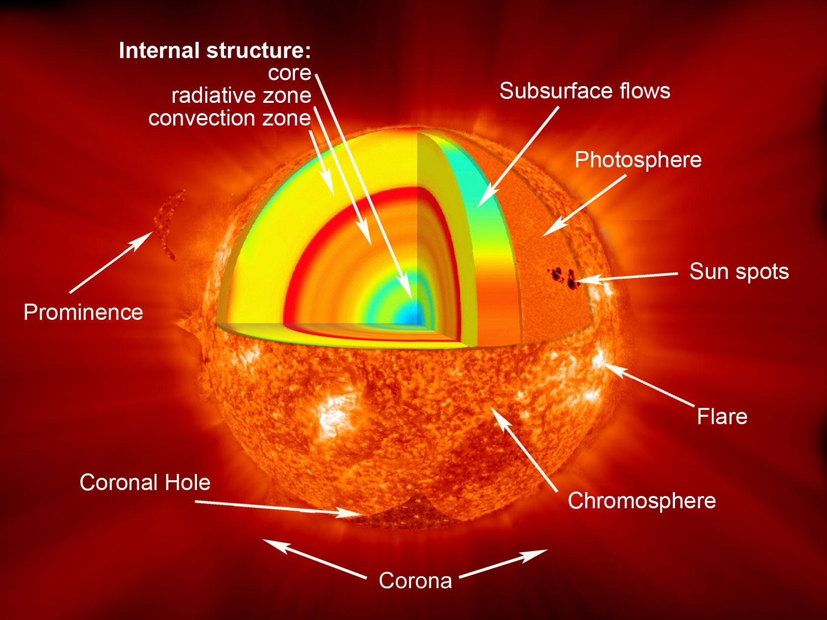
Figure 3.1: The layers of the Sun (Credit: NASA, 2017)

The core of the Sun is 25$\%$ of the solar radius (García et al., 2007), the density is about $150g/cm^{3}$ (Basu et al., 2009) contains 34$\%$ of the solar mass even though only 0.8$\%$ of the total volume, and it is the hottest part of the Sun that a temperature of 15 million Kelvins (Dr. David H. Hathaway, 2015). This is the zone where the thermonuclear reaction is going. For the radiative zone, it starts from the edge of the core to the interface layer (tachocline), and much of the energy generated in the core is carried away by photons though photons take a million years to reach the next layer due to the dense material of the region (Chemin, 2022).

The very next layer, the interface layer (tacholine) is much of our interest because it is believed that the solar magnetic dynamo originates in this very thin layer (Tobias and Weiss, 2007) that magnetic field lines can become stronger due to the changes in the fluid flow velocities crossing this layer. However, recent radio observations of brown dwarf stars show that, despite not having a tachocline layer, they can have similar magnetic strength and activities just like the Sun, which indicates the convection zone may be solely responsible for the solar dynamo (Route, 2016).

Next, the convection zone is the outermost layer of the inner zones and it extends about 200,000 km from the depth and the temperature is approximately 2 million Kelvins (Christensen-Dalsgaard et al., 1991), which makes the zone relatively cooler for heavy ions to keep their electrons so that the zone is opaque to the radiation (Ortuño-Araujo et al., 2012), which in turn traps the heat and eventually the fluid becomes unstable and start convecting. As a result, this layer is very turbulent (Brummell et al., 1995), which in addition to the rotational motion creates electric currents and magnetic fields, and the gas pressure is much more dominant than the magnetic pressure in this region, and because of this the magnetic field is dragged and twisted by the fluid, which then propagates passing through the photosphere, chromosphere, the transition region up to the corona and creates a multitude of activities on the surface of the Sun called solar activity.

In the photosphere, visible darker areas called sunspots appear due to localized strong magnetic regions, which inhibit some of the heat from reaching the surface and this makes the areas cooler than the other parts of the Sun (Babcock and Babcock, 1955). Because of the mentioned strong magnetic nature, the magnetic field lines around the sunspot often twist and cross, causing a tension of energy that bursts in an explosion called a solar flare (Chakraborty and Basak, 2022).

The corona is the hot and ionized outermost layer of the Sun and it is millions of Kelvins greater than that of the surface of the Sun (Aschwanden, 2006). The solar magnetic field confines much of the coronal plasma, but some of the plasma spread with a supersonic speed into interplanetary space, which is called the solar wind. The solar magnetic field forms so-called flux tubes. These ropes are tensed by the differential rotation of the Sun. Therefore, store plenty of energy. If a certain configuration appears (X-shape) the magnetic structure reorganizes. Hence, a huge amount of energy is released. The name of this 20 million K-degree flash is a solar flare. It emits plenty of energized protons and other ions in the heliosphere and very often, but not always a huge amount of solar plasma ejects to the IP space. The process is called coronal mass ejections (CME). However, CME could occur without a flare too. These phenomena are the main drivers of space weather and the conditions of the terrestrial cosmic environment (Facskó et al., 2022). The solar activity is cyclic, which is called the solar cycle, and it is approximately 11 years (Center/SDO, 2015), see Figure 3.2. Each cycle the magnetic field of the Sun flips, and the periods, in which, the sunspots are the greater in number are called solar maximum and the lower in number are called solar minimum.

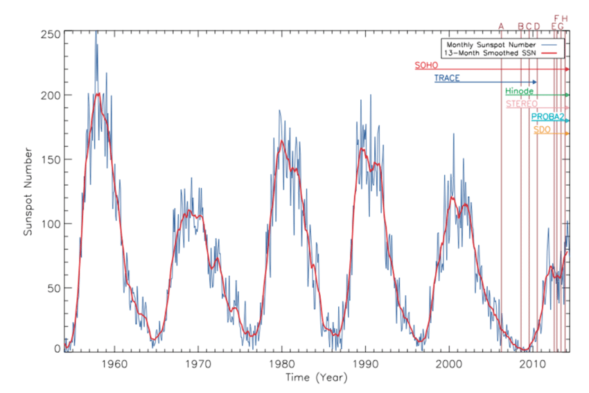
Figure 3.2: The sunspot cycle over the last several decades (Figure is from Pasachoff et al., 2014; Figure 8)

3.2 The Solar Wind and the Interplanetary Magnetic Field

The Sun ejects highly energized and ionized charged particles continuously in all directions, which is the solar wind. The solar wind is a collisionless plasma that consists of equal amounts of protons and electrons with the addition of negligible 3 to $6\%$ helium (Neugebauer, 1981). As a result, the solar wind is a quasi-neutral plasma whose characteristics can be defined by magnetohydrodynamics (MHD). In MHD, Alfvén theorem states that in a fluid with high electric conductivity the magnetic field line is frozen in it and moves along with it (Alfvén, 1942). Since the solar wind is one such fluid the Sun’s magnetic field lines are frozen in the flow that they are forced to propagate with the solar wind (Roberts, 2007), forming the interplanetary magnetic field (IMF). Depending on the origination point whether in the coronal holes or the equatorial belt of the Sun, the solar wind is classified as the fast solar wind with a velocity of 750 km/s and the slow solar wind with a velocity of 400 km/s respectively (Feldman et al., 2005). The coronal holes are areas that appear dark in X-ray images because these areas are much cooler and less dense than other regions (Cranmer, 2009) and the magnetic field around these areas does not loop back down but extends into the interplanetary space (Parker, 1959), so the plasma can easily flow out, creating the fast solar wind. The coronal holes can appear anywhere on the coronal areas during the solar maximum while they usually appear on northern or southern poles of the sun during the solar minimum (McComas et al., 2003).

Figure 3.3: Combined X-ray image of the Sun’s active regions observed from several telescopes. High-energy X-rays from NASA’s Nuclear Spectroscopic Telescope Array (NuSTAR) are shown in blue, low-energy X-rays from Japan’s Hinode spacecraft are green, and extreme ultraviolet light from NASA’s Solar Dynamics Observatory (SDO) is yellow and red (Credit: NASA/JPL-Caltech/GSFC/JAXA, 2015)

The expansion of the solar wind is a radial propagation away from the Sun that it is diluted and cools down on its journey. As seen from some observations the density of the solar wind decreases approximately as $r^{-2}$ while the temperature decrease is less significant about a factor of 20 (Baumjohann and Treumann, 2012). During the expansion of the radial flow, the Sun rotates, which is 27 days on average, and because the magnetic field lines are anchored in the sun, the radial flow looks like an Archimedean spiral called the Parker Spiral. At 1 AU the spiral makes $45^{0}$ to the Earth-Sun line, see Figure 3.4.

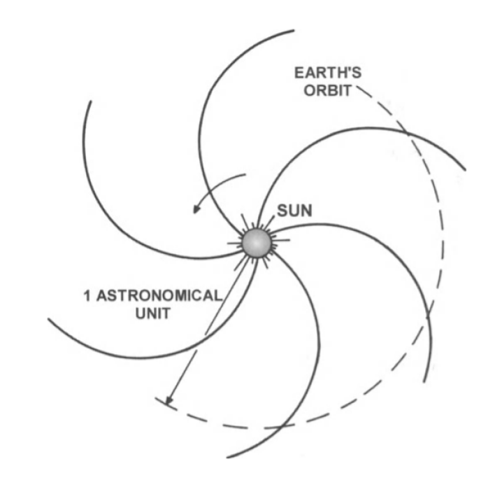
Figure 3.4: Schematic representation of the Archimedes spiral structure of the interplanetary magnetic field (Figure is from Bittencourt, 2004; Figure 3)

The solar wind travels throughout the solar system and defines the heliosphere the region in space whose frontier is impeded by the interstellar medium. Consequently, the heliosphere is a giant bubble whose center is the Sun and protects the solar system from interstellar radiations and cosmic rays. The size of the heliosphere is about 121 AU (Cowen, 2013). The solar wind decelerates when it flows outward through the Solar System. At a certain point, the flow becomes subsonic and forms a shock. Its name is termination shock (Jokipii, 2013). Then the flow continues its journey outward and interacts with the interstellar material. It is under debate whether the speed of the Solar System is super- or sub-sonic. A bow shock or bow wave forms before the heliosphere, respectively. Furthermore, due to the interaction, the solar wind becomes turbulent and this region is called heliosheath which is in between the termination shock and the heliopause (Burlaga, 2015).

3.3 Interplanetary shocks

The average interplanetary magnetic field strength is around 6 nT at 1 AU (Lowrie and Fichtner, 2020) and considering the average speed of the solar wind, the solar wind is both supersonic and super-Alfvénic, which means it is super-magnetosonic. As a result of this nature of the solar wind, when it collides with celestial objects such as planets, moons, asteroids, and comets or its slow-flowing part, shocks are formed. The main characteristic of shocks that can be found in interplanetary space to interstellar regions is a denser state in contrast to the medium in which they propagate due to the shock formation. Furthermore, if the celestial objects are magnetized, then the shock formations create interesting interaction regions, and their physics looks very exciting.

One such fascinating magnetized object is our planet, the Earth. The Earth has its magnetic field, known as the magnetosphere, which originated from its inner core via the dynamo effect (Gilbert, 2003). The Earth’s magnetosphere extends 60000 kilometers in the sunward direction while a million kilometers in the anti-sunward direction (Lakhina et al., 2009). Such a big extension is a common characteristic of all the magnetized planets, and as a result of this extension, the cross-section of a planet is increased by a large factor. For example for the Earth, the factor is 150 (Baumjohann and Treumann, 2012). The magnetic field frozen in the supersonic and super-Alfvénic solar wind plasma cannot enter the magnetosphere, the region where the terrestrial magnetosphere dominates. As a result, a special standing wave, the bow shock forms (Baumjohann and Nakamura, 2007). (3.5).

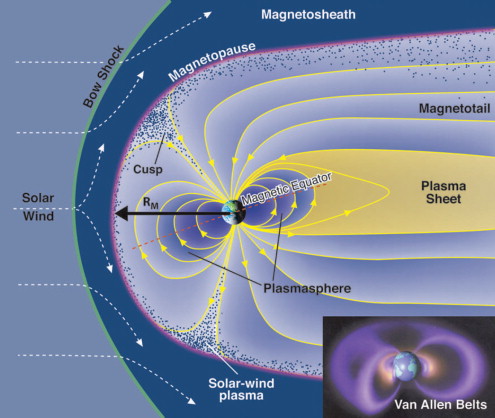
Figure 3.5: Illustration of the Earth’s magnetosphere and its interaction with the solar wind. (Figure is from Kivelson and Bagenal, 2007; Figure 1)

Consequence of the slowing down of the solar wind plasma, the kinetic energy of some of the particles is converted into thermal energy, which occurs behind the bow shock, and this region is called the magnetosheath. The boundary region between two magnetic field lines is called the magnetopause. Bow shock formation is common to all the planets and celestial objects with or without magnetospheres (Mazelle et al., 2004).

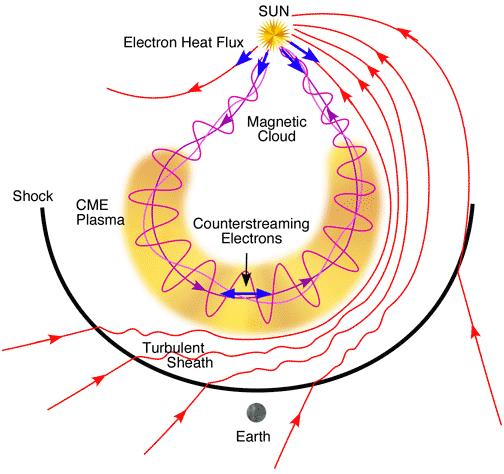
Figure 3.6: Illustration of a CME event. (Credit: NASA, 2017)

In addition, there are several other shocks, the previously mentioned termination shock, coronal mass ejection (CME) driven shock, and a co-rotating interaction region (CIR) driven shock. When a CME event occurs, it moves faster than the background solar wind flow, resulting in a shock wave. On the created shock waves charged particles accelerate. So usually CMEs are one of the main causes of the solar energetic particles (SEPs) (Cane and Lario, 2006), see Figure 3.6.

Similarly to the shocks caused by CMEs, When the fast-moving solar wind flow catches the slow-moving solar wind flow, the so-called co-rotating interaction region is formed, and if the pressure gradient gets sufficiently large and the speed difference surpasses the local speed shocks can arise (Heber et al., 1999), Figure 3.7.

Figure 3.7: Co-rotating interaction region. (Figure is from David Burgess, 2017)

3.3.1 Classifications of Interplanetary (IP) shocks

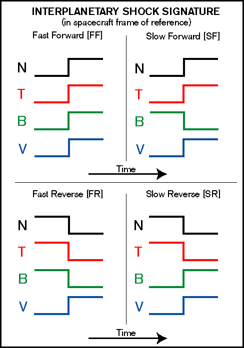
Figure 3.8: Categorizations of IP shocks. N, T, B, and V denote number density, the proton temperature, the magnitude of the magnetic field, and speed respectively. (Figure is from WIND MFI Team Science, 2001)

Armed with the above shock definitions and categorizations knowledge, now we can finally be able to classify IP shocks. The IP shocks can be classified based on their travel directions concerning the solar wind frame of reference. If the shock is moving away from its driver, here the Sun is referred but drivers can be detailed such as ICMEs, CIRs, etc, the shock is called forward shock (FS), and if it is moving toward its driver, it is called reverse shock (RS). Adding the previous definitions of fast and slow shocks, IP shocks are usually categorized as fast forward (FF), fast reverse (FS), slow forward (SF) and slow reverse (SR) shocks (Berdichevsky et al., 2000), see Figure 3.8. As you can see from Figure 3.8, the solar wind plasma parameters – number density N, the proton temperature T, the magnitude of the magnetic field B, and the bulk speed V parameters increase dramatically from upstream (unshocked) to downstream (shocked) regions in fast forward (FF) shocks while the parameters except for the bulk speed decrease in fast reverse (FR) shocks. In the case of slow forward (SF) shocks, the parameters except for the magnitude of the magnetic field increase from upstream to downstream whereas in the case of slow reverse (SR) shocks, the number density N and the proton temperature T decrease while the magnitude of magnetic field B and the bulk speed V increase.

Within 1 AU, the most frequent IP shocks are fast forward (FF) shocks (Richter et al., 1985)

Chapter 4 Analysis methods

4.1 Instruments

In this thesis, Solar Terrestrial Relations Observatory (STEREO) A and B, Wind, Advanced Composition Explorer (ACE), and the Cluster spacecraft magnetic field and ion plasma data are used. In the following subsections, the basic descriptions of each spacecraft, its orbits, and its instruments are mentioned.

4.1.1 The STEREO mission

The twin Solar Terrestrial Relations Observatory (STEREO) A and B spacecraft were launched on October 26, 2006, from Kennedy Space Center (Kaiser et al., 2008). In heliospheric orbit at 1 AU, STEREO$-$A (Ahead) leads while STEREO$-$B (Behind) trails Earth. The two spacecraft separate at $44^{\circ}$ from each other annually, see Figure 4.1. This formation allows the stereoscopic image of the Sun from the Sun-Earth axis angle in 3D. The purposes of the mission are to study the cause and initiation mechanisms of coronal mass ejection (CME) and their propagation through the heliosphere, discover the sites and procedures of solar energetic particles in the corona as well as the interplanetary medium, and construct a three dimensional and time-dependent model of the parameters of the solar wind (Kaiser, 2005).

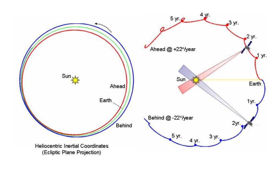
Figure 4.1: Left panel shows the orbits of STEREO$-$A and B relative to that of Earth. The right panel shows the degree of separation of two spacecraft in years from their first launch period. (Figure is from Kaiser, 2005; Figure 2)

The two spacecraft are each equipped with the complement of four scientific instruments, particularly two instruments and two instrument suites, with a total of 13 instruments on each spacecraft. The complements of the four instruments are as follows:

• 1. Sun-Earth Connection Coronal and Heliospheric Investigation (SECCHI)

• 2. STEREO/WAVES (S/WAVES)

• 3. In situ Measurements of Particles and CME Transients (IMPACT)

• 4. Plasma and Suprathermal Ion Composition (PLASTIC)

The SECCHI suite of instruments has two white light coronagraphs, an extreme ultraviolet imager, and two heliospheric white light imagers for tracking CMEs (Howard et al., 2008). S/WAVES instrument utilizes radio waves to trace locations of the CME-driven shocks and the 3-D open field lines for the particles created by solar flares (Bougeret et al., 2008). The PLASTIC instrument measures proton, the composition of heavy ions, and alpha particles in the solar wind plasma (Galvin et al., 2008). The IMPACT suite of instruments consists of seven instruments, and three of them are located on the 6-meter boom as shown in Figure 4.2 while the others are in the main hull of the spacecraft (Acuña et al., 2008). The IMPACT measures protons, heavy ions, and electrons, and the MAG magnetometer sensor in it measure the in situ magnetic fields in a range of $\pm 512nT$ with 0.1 nT accuracy (Kaiser and Adams, 2007).

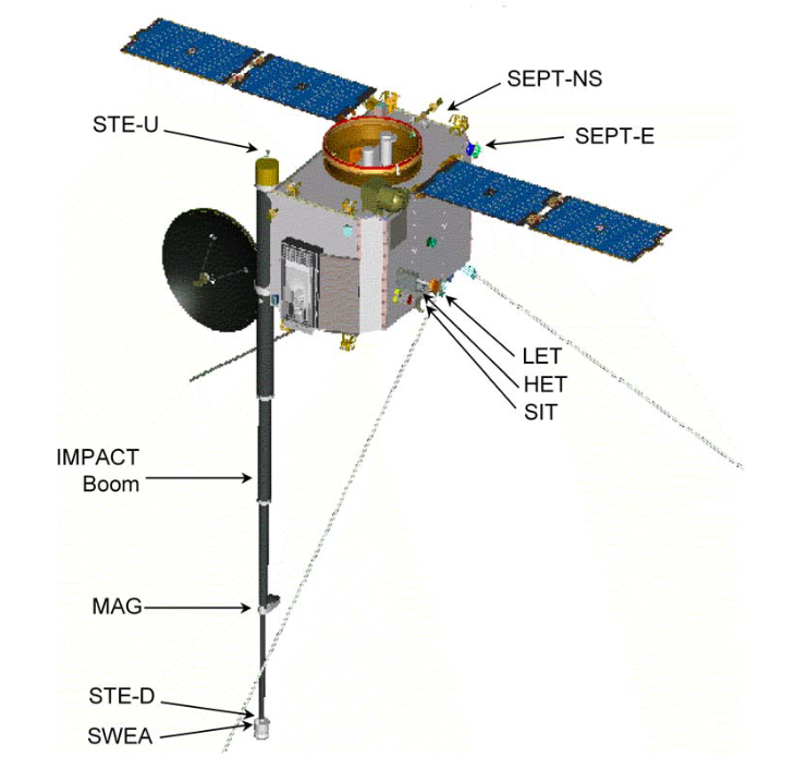
Figure 4.2: Relative placement of the IMPACT boom on the STEREO (Figure is from Acuña et al., 2008; Figure 1)

Unfortunately, multiple hardware issues affecting control of the spacecraft resulted in the loss of contact with STEREO$-$B on October 1, 2014, (STEREO Science Center, 2018).

4.1.2 Wind

NASA’s Wind spacecraft was launched on November 1, 1994, (Wilson III et al., 2021). The Wind was initially planned sent to $L_{1}$ Lagrangian point but was delayed to study the magnetosphere and lunar environment. Following a sequence of orbital adjustments, the Wind spacecraft was positioned in a Lissajous orbit close to the $L_{1}$ Lagrange point in early 2004 for studying the incoming solar wind on the verge of impacting Earth’s magnetosphere (NASA WIND team, 2020), see Figure 4.3.

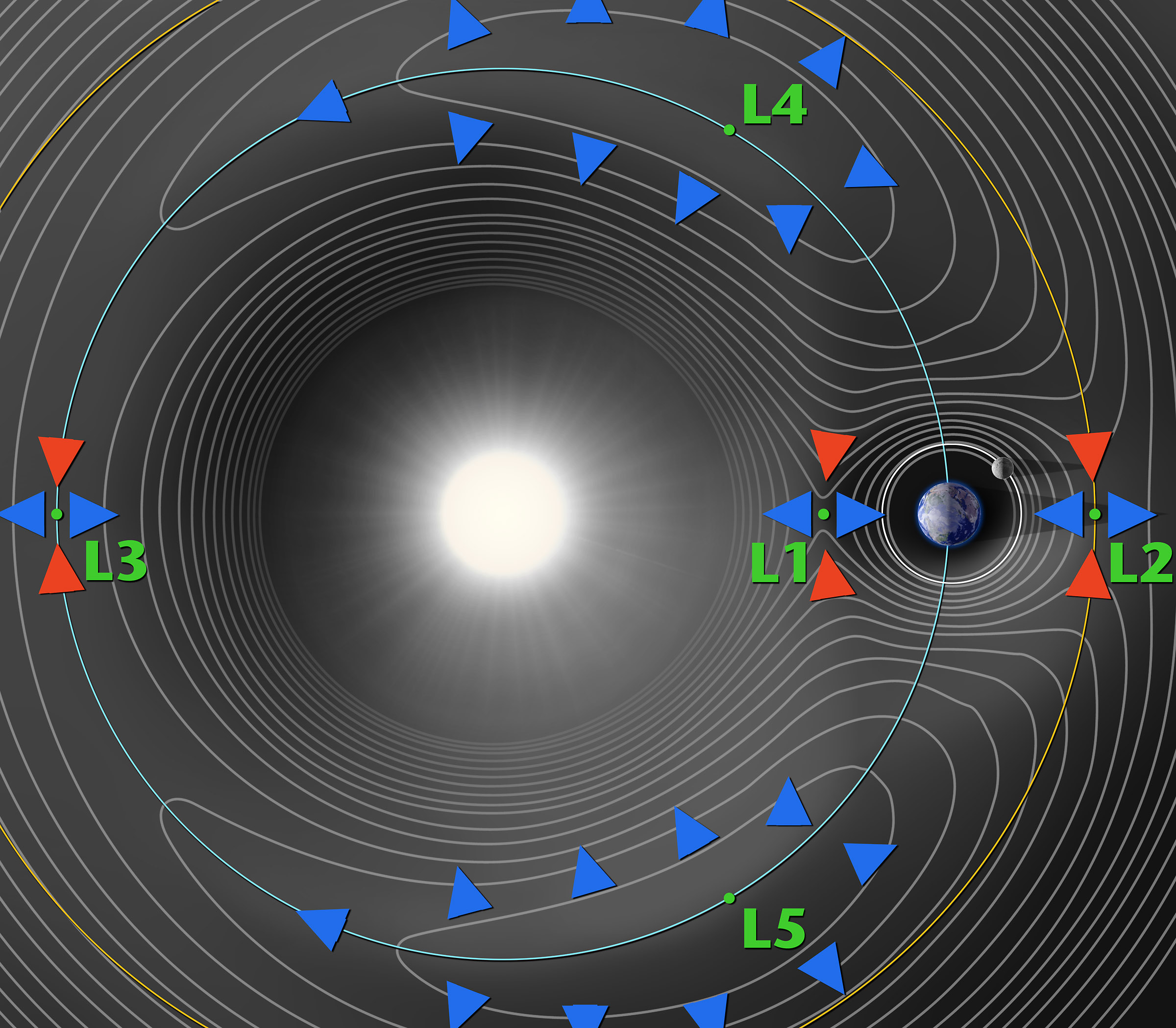
Figure 4.3: Lagrangian points in the Sun-Earth system. (Credit: NASA Solar System Exploration, 2020)

The object of the mission is to study solar wind plasma, magnetic field, and solar and cosmic energetic particles. The spacecraft is equipped with the eight instruments such as Solar Wind Experiment (SWE Ogilvie et al., 1995), 3-D plasma (3DP Wilson III, 2011), Magnetic Field Investigation (MFI Lepping et al., 1995), Solar wind/mass suprathermal ion composition studies (SMS Gloeckler et al., 1995), Energetic Particles: Acceleration, Composition Transport (EPACT Von Rosenvinge et al., 1995), Radio and Plasma Wave Experiment (WAVES Bougeret et al., 1995), (KONUS Mazets and Golenetskii, 1981) and Transient Gamma-Ray Spectrometer (TGRS Owens et al., 1991), see Figure 4.4. From these instruments, MFI and SWE are of interest to this thesis. The MFI consists of two magnetometers at the 12-meter boom, its measurement capability is 4 nT, 65536 nT, and measures vector magnetic field up in a time resolution of 22 or 11 vectors per second for the calibrated high-resolution data and primary science data is in time resolutions of three seconds, one minute and one hour (NASA WIND team, 2022). The SWE measures the solar wind key parameters such as velocity, density, and temperature.

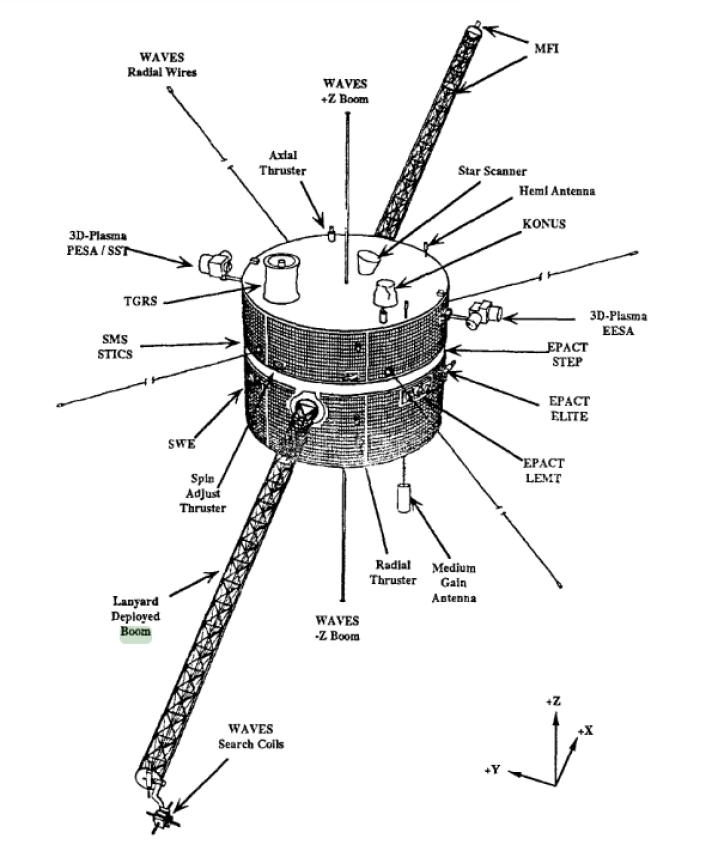
Figure 4.4: Configuration of the Wind instruments. (Figure is from Harten and Clark, 1995; Figure 1)

4.1.3 ACE

NASA’s ACE spacecraft was launched on August 25, 1997, (Stone et al., 1998c). The spacecraft is located at $L_{1}$ Lagrangian point same as the Wind spacecraft, see Figure 4.3. The general purposes of ACE are to gather and study particles originating from the sun, interplanetary or interstellar mediums, and the galaxy as well as to investigate the solar wind structures such as ICMEs and magnetic clouds. The spacecraft is equipped with nine primary scientific instruments and one engineering instrument such as Cosmic-Ray Isotope Spectrometer (CRIS Stone et al., 1998a), Electron, Proton, and Alpha-particle Monitor (EPAM), Magnetometer (MAG Smith et al., 1998), Real-Time Solar Wind (RTSW Zwickl et al., 1998), Solar Energetic Particle Ionic Charge Analyzer (SEPICA Mobius et al., ), Solar Isotope Spectrometer (SIS Stone et al., 1998b), Solar Wind Electron, Proton and Alpha Monitor (SWEPAM McComas et al., 1998), Solar Wind Ion Composition Spectrometer (SWICS) and Solar Wind Ion Mass Spectrometer (SWIMS Gloeckler et al., 1998) and Ultra-Low-Energy Isotope Spectrometer (ULEIS Mason et al., 1998), see Figure 4.5. The MAG consists of twin triaxial flux-gate magnetometers such that magnetometer sensors have between 3 and 6 vectors $s^{-1}$ resolutions for continuous observation of the interplanetary magnetic field (Smith et al., 1998).

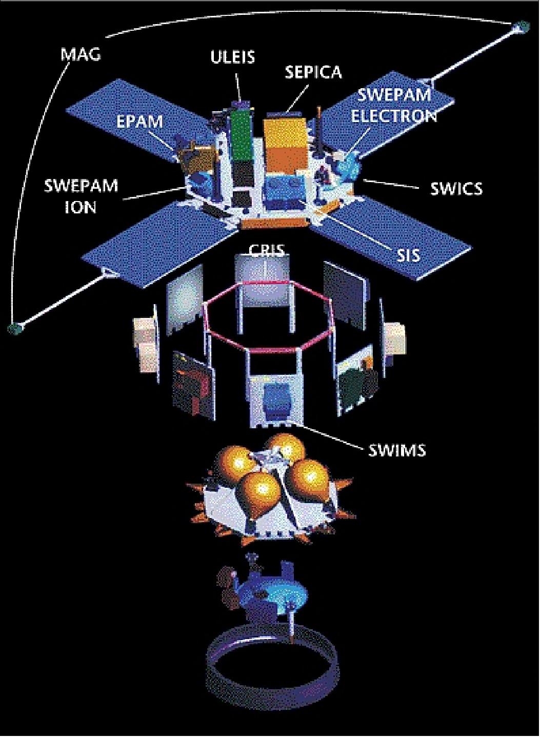
Figure 4.5: Instruments of ACE spacecraft. (Figure is from Stone et al., 1998c; Figure 6)

4.1.4 Cluster

ESA’s Cluster constellations consist of 4 satellites, which were launched on 16 July and 9 August 2000 (Escoubet et al., 2001). The Cluster satellites orbit in a tetrahedral formation around Earth. The orbits feature perigees close to 4 Earth radii ($R_{E}$) and apogees approximately 19.6 $R_{E}$ away (Zhang et al., 2010). The primary objectives of the Cluster mission involve examining small-scale plasma formations and macroscopic turbulences in three dimensions in crucial plasma areas, including solar wind, bow shock, magnetopause, polar cusps, magnetotail, and auroral regions (Escoubet et al., 2001). The four satellites are each equipped with 11 instruments such as Active Spacecraft Potential Control (ASPOC Torkar et al., 2016), Ion Composition (CIS Reme et al., 1997), Electron Drift Instrument (EDI Haaland et al., 2007), Fluxgate Magnetometer (FGM Balogh et al., 1997), Plasma Electron And Current Experiment (PEACE Johnstone et al., 1997), Research with Adaptive Particle Imaging Detectors (Daly and Kronberg, 2010; RAPID), Digital Wave processor (DWP Woolliscroft et al., 1997), Electric field and waves (EFW Gustafsson et al., 1997), Spatio-Temporal Analysis of Field Fluctuations (STAFF Cornilleau-Wehrlin et al., 1997), Wide-band plasma wave (WBD Gurnett et al., 1997), and Waves of High frequency and Sounder for Probing of Electron Density (WHISPER Décréau et al., 1997) as shown in Figure 4.6. From the instruments, the magnetic and plasma parameters are up to our interest. Hence, the FGM magnetometer, CIS, and EFW instruments are emphasized. The Fluxgate Magnetometer (FGM) is composed of two tri-axial fluxgate magnetometers, which are installed on one of the two 5-meter radial booms. It measures in the dynamic range $\pm 65,536$nT. At the highest dynamic level, the resolution is $\pm 8$ nT, and the time resolution is 100 vectors per second (Organization, 2021). CIS (Ion composition) instrument measures three-dimensional ion distribution, and it is composed of two distinct sensors: the Composition Distribution Function (CODIF) sensor and the Hot Ion Analyzer (HIA) sensor. The CIS experiment is not operational for Cluster-2 and the HIA sensor is switched off for Cluster-4 due to a problem with the high voltage of the electrostatic analyzer (CIS team, 2021). Hence, for Cluster-2 and Cluster-4, the Electric Field and Wave (EFW) instrument measurement is useful. The EFW instrument measures the electric field fluctuations as well as the spacecraft potential, which is essential for studying plasma density and spacecraft charging.

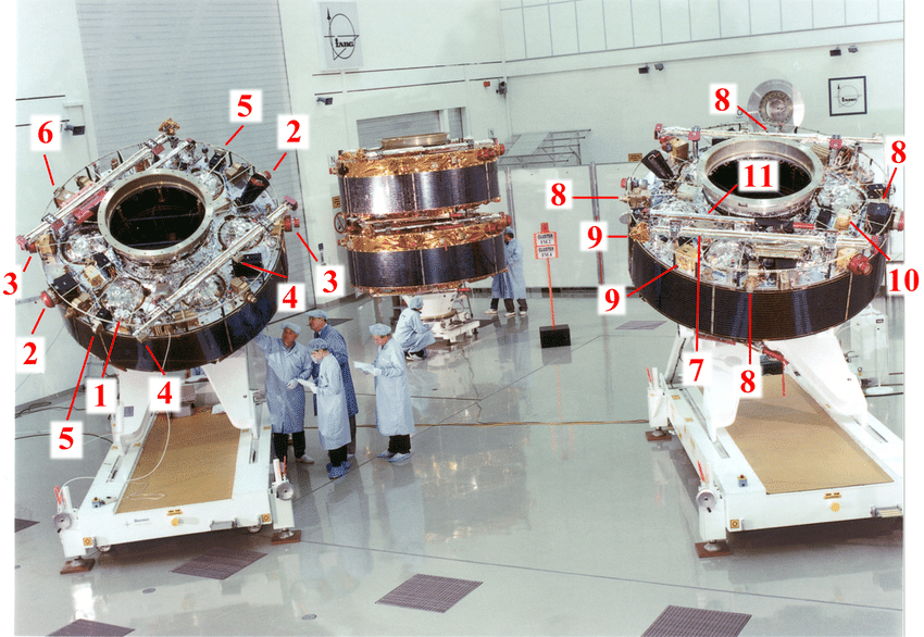
Figure 4.6: Instruments on Cluster satellites. ASPOC (1), CIS (2), EDI (3), FGM (4), PEACE (5), RAPID (6), DWP (7), EFW (8), STAFF (9), WBD (10), WHISPER (11) (Figure is from Escoubet et al., 2001; Figure 3)

4.2 Methods

The following two methods are suitable for single-spacecraft measurements and both of them are based on the divergence of the magnetic field, $\nabla\cdot\mathbf{B}=0$, constraint, and both of them use solely magnetic field data. The following formalization, descriptions, and derivations are based on (Sonnerup and Scheible, 1998) and (Paschmann and Daly, 2000).

4.2.1 Minimum Variance Analysis

The Minimum variance analysis technique was first developed by (Sonnerup and Cahill Jr, 1967). It is based on the assumption that variations in the magnetic field would be observed when a single spacecraft passes through a 1-D current layer or wavefront. Remembering the divergence of the magnetic field constraint, $\nabla\cdot\mathbf{B}=0$, such that the normal component of the magnetic field must remain constant. If such a normal direction can be found, then the variations in the magnetic field are zero or at the least has a minimum variance. Thus, $\mathbf{\hat{\textbf{n}}}$ can be determined by the minimization of the following equation:

$$\sigma^{2}=\frac{1}{M}\sum_{m=1}^{M}\bigg{|}(\mathbf{B}^{(m)}-\langle\mathbf{B}\rangle)\cdot\mathbf{\hat{\textbf{n}}}\bigg{|}^{2},$$ (4.1)

where ${\mathbf{B}^{(m)}},(m=1,2,3...M)$ is the magnetic field in a time series data and $\mathbf{B}$ is the average magnetic field.

Taking the account of the normalization constraint $|\mathbf{\hat{\textbf{n}}}|^{2}=1$, on which minimization is conditioned, and introducing a Lagrange multiplier, $\lambda$, for utilizing the constraint, the solution of three homogeneous linear equations can be found. The three homogeneous equations are:

$$\frac{\partial}{\partial n_{X}}\bigg{(}\sigma^{2}-\lambda|\mathbf{\hat{\textbf{n}}}|^{2}-1\bigg{)}=0$$ (4.2)

$$\frac{\partial}{\partial n_{Y}}\bigg{(}\sigma^{2}-\lambda|\mathbf{\hat{\textbf{n}}}|^{2}-1\bigg{)}=0$$

$$\frac{\partial}{\partial n_{Z}}\bigg{(}\sigma^{2}-\lambda|\mathbf{\hat{\textbf{n}}}|^{2}-1\bigg{)}=0,$$

where $\sigma^{2}$ is given by 4.1 and $\mathbf{\hat{\textbf{n}}}$ is expressed in its three components, which are along X, Y, and Z coordinates. After the differentiation procedures of 4.2 are done, the resulting sets of equations can be written in matrix form:

$$\sum_{\nu=1}^{3}M_{\mu\nu}n_{\nu}=\lambda n_{\mu},$$ (4.3)

where the subscripts $\mu$ and $\nu$ indicate cartesian coordinates and $M_{\mu\nu}$ is the magnetic variance matrix:

$$M_{\mu\nu}n_{\nu}=<B_{\mu}B_{\nu}>-<B_{\mu}><B_{\nu}>$$ (4.4)

with $\lambda$ being the eigenvalues with three possible values $\lambda_{1}$, $\lambda_{2}$, and $\lambda_{3}$ with decreasing order. The eigenvalues have their corresponding eigenvectors $\mathbf{x_{1}}$, $\mathbf{x_{2}}$, and $\mathbf{x_{3}}$ of the matrix where they represent the directions of maximum, intermediate, and minimum variance of the magnetic field component. The eigenvectors corresponding to the smallest value of the $\lambda$ eigenvalues are the shock normal vectors. The eigenvalue ratios, especially intermediate to minimum eigenvalue ratio, must be greater than 2 or 3 to keep the variance space ellipsoid (Paschmann and Daly, 1998) as shown in Figure 4.7

Figure 4.7: The illustration of the variance space ellipsoid geometry (Figure is from Rosa Oliveira et al., 2020; Figure 1)

4.2.2 The Magnetic Coplanarity method

If two vectors that lie inside a coplanar surface can be determined, the normal to the coplanar surface can be found.

The coplanarity methods are based on the magnetic coplanarity theorem, which stated that both sides of the magnetic field vectors on the shock and the shock normal lie in the same plane. Similarly, the velocity on both sides or, in other words, the velocity jump through the shock also lie in the same plane. The upstream and downstream magnetic fields and velocities satisfy the Rankine-Hugionot conditions. So, there are multiple vectors lie in the shock plane, and the resulting constraint equations are as follows:

$$(\mathbf{B}_{down}-\mathbf{B}_{up})\cdot\mathbf{\hat{\textbf{n}}}=0$$ (4.5)

$$(\mathbf{B}_{down}\crossproduct\mathbf{B}_{up})\cdot\mathbf{\hat{\textbf{n}}}=0$$ (4.6)

$$(\mathbf{B}_{up}\crossproduct(\mathbf{V}_{down}-\mathbf{V}_{up}))\cdot\mathbf{\hat{\textbf{n}}}=0$$ (4.7)

$$(\mathbf{B}_{down}\crossproduct(\mathbf{V}_{down}-\mathbf{V}_{up}))\cdot\mathbf{\hat{\textbf{n}}}=0$$ (4.8)

$$((\mathbf{B}_{up}-\mathbf{B}_{down})\crossproduct(\mathbf{V}_{down}-\mathbf{V}_{up}))\cdot\mathbf{\hat{\textbf{n}}}=0,$$ (4.9)

where the indexes up and down denote upstream and downstream, respectively. From 4.5 and 4.6 the magnetic coplanarity normal is defined:

$$\mathbf{\hat{\textbf{n}}}_{MC}=\pm\frac{(\mathbf{B}_{down}\crossproduct\mathbf{B}_{up})\crossproduct(\mathbf{B}_{down}-\mathbf{B}_{up})}{\absolutevalue{(\mathbf{B}_{down}\crossproduct\mathbf{B}_{up})\crossproduct(\mathbf{B}_{down}-\mathbf{B}_{up})}},$$ (4.10)

where the signs are arbitrary.

The magnetic coplanarity schematic illustration is shown in Figure 4.8.

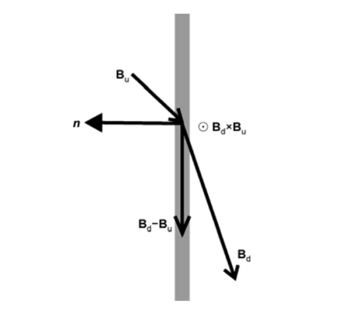
Figure 4.8: The illustration of the magnetic coplanarity. The gray vertical line represents the shock layer. (Figure is from Shan et al., 2013; Figure 1)

Similarly, from 4.7, 4.8 and 4.9 the mixed modes for normals can be defined, respectively.

$$\mathbf{\hat{\textbf{n}}}_{mix1}=\pm\frac{(\mathbf{B}_{up}\crossproduct(\mathbf{V}_{down}-\mathbf{V}_{up}))\crossproduct(\mathbf{B}_{down}-\mathbf{B}_{up})}{\absolutevalue{(\mathbf{B}_{up}\crossproduct(\mathbf{V}_{down}-\mathbf{V}_{up}))\crossproduct(\mathbf{B}_{down}-\mathbf{B}_{up})}}$$ (4.11)

$$\mathbf{\hat{\textbf{n}}}_{mix2}=\pm\frac{(\mathbf{B}_{down}\crossproduct(\mathbf{V}_{down}-\mathbf{V}_{up}))\crossproduct(\mathbf{B}_{down}-\mathbf{B}_{up})}{\absolutevalue{(\mathbf{B}_{down}\crossproduct(\mathbf{V}_{down}-\mathbf{V}_{up}))\crossproduct(\mathbf{B}_{down}-\mathbf{B}_{up})}}$$ (4.12)

$$\mathbf{\hat{\textbf{n}}}_{mix3}=\pm\frac{((\mathbf{B}_{down}-\mathbf{B}_{up})\crossproduct(\mathbf{V}_{down}-\mathbf{V}_{up}))\crossproduct(\mathbf{B}_{down}-\mathbf{B}_{up})}{\absolutevalue{((\mathbf{B}_{down}-\mathbf{B}_{up})\crossproduct(\mathbf{V}_{down}-\mathbf{V}_{up}))\crossproduct(\mathbf{B}_{down}-\mathbf{B}_{up})}}$$ (4.13)

From these, the equation 4.10 is used and as denoted further on as (CP). The method of magnetic coplanarity is straightforward to implement and, as previously mentioned, it only necessitates the use of a magnetic field data (Paschmann and Daly, 1998).

4.2.3 The Utilization of the Methods

By comparing the two methods, the upstream and downstream time intervals of the magnetic field measurements are set. In this thesis work, as stated before the magnetic coplanarity method 4.10 is used out of the other coplanarity methods.

To accept the intervals, there are some criteria to be put in such as:

• The angle between the vectors defined by the minimum variance analysis (MVA) and the magnetic coplanarity method must be less than $15^{\circ}$ (Facskó et al., 2008, 2009, 2010).

• The ratio between the intermediate eigenvalue and the smallest eigenvalue should be greater than 2 (Facskó et al., 2008, 2009, 2010), the same for more data points and greater than 10 for data points less than 50 Sonnerup and Cahill Jr (1967) or the ratio between the smallest eigenvalue to the intermediate eigenvalue should be smaller than 1/3 (Shan et al., 2013), which is in reverse means greater than 3.

4.2.4 Estimating the solar wind parameters

The following parameter estimations are based on this paper (Lumme et al., 2017)

Shock criteria:

The solar wind bulk speed jump should fulfill the following conditions:

$$V_{down}-V_{up}\geq 20\quad\text{km/s for FF}\quad\text{and}\quad V_{up}-V_{down}\geq 20\quad\text{km/s for FR}$$ (4.14)

And downstream to upstream ratios should fulfill the following ratios of upstream and downstream the magnetic field, density, and temperature respectively:

$$\frac{B_{down}}{B_{up}}\geq 1.2\quad\frac{N^{down}_{p}}{N^{up}_{p}}\geq 1.2\quad\text{and}\quad\frac{T^{down}_{p}}{T^{up}_{p}}\geq\frac{1}{1.2}$$ (4.15)

Shock theta:

This is the angle between the normal vector $\mathbf{\hat{\textbf{n}}}$ and the upstream magnetic field lines:

$$\theta_{Bn}=cos^{-1}\bigg{(}\absolutevalue{\frac{\mathbf{B}_{up}\cdot\mathbf{\hat{\textbf{n}}}}{|\mathbf{B}_{up}||\mathbf{\hat{\textbf{n}}}|}}\bigg{)}$$ (4.16)

Shock speed:

The shock speed in the spacecraft frame of reference:

$$V_{sh}=\bigg{|}\frac{N^{up}_{p}\mathbf{V}_{up}-N^{down}_{p}\mathbf{V}_{down}}{N^{down}_{p}-N^{up}_{p}}\cdot\mathbf{\hat{\textbf{n}}}\bigg{|}$$ (4.17)

Upstream sound speed:

$$C^{up}_{s}=\bigg{<}\sqrt{\gamma k_{B}\frac{T_{p}+T_{e}}{m_{p}}}\bigg{>},$$ (4.18)

where $m_{p}$ is the proton mass, $T_{p}$ and $T_{e}$ are proton and electron temperature. In the solar wind, the electron temperature at 1 AU is assumed to be $\sim 140,000$ K (Newbury, 1996).

Upstream Alfvén speed:

$$V^{up}_{A}=\bigg{<}\frac{B}{\sqrt{\mu_{0}N_{p}m_{p}}}\bigg{>},$$ (4.19)

where $\mu_{0}$ is the magnetic vacuum permeability, $N_{p}$ is the proton density and $m_{p}$ is the proton mass.

Upstream magnetosonic speed:

The equation 2.25 is used for here

Upstream plasma beta:

$$\beta^{up}=\bigg{<}\frac{2\mu_{0}k_{B}N_{p}(T_{p}+T_{e})}{B^{2}}\bigg{>}$$ (4.20)

Alfvén Mach number:

$$M_{A}=\frac{|\mathbf{V}_{up}\cdot\mathbf{\hat{\textbf{n}}}\pm\mathbf{V}_{sh}|}{V^{up}_{A}},$$ (4.21)

where $V_{up}$ is the upstream velocity, $V_{sh}$ is shock speed and $V^{up}_{A}$ is the Alfvén speed. The reason for $\pm V_{sh}$ is a Galilean coordinate transformation to the shock rest frame. The sign $\pm$ is depend on FF shock, for which (-) or FR shock, for which (+).

Magnetosonic Mach number:

Similarly to 4.21 the Magnetosonic Mach number is defined as follows:

$$M_{ms}=\frac{|V_{up}\cdot\mathbf{\hat{\textbf{n}}}\pm V_{sh}|}{C_{ms}},$$ (4.22)

where $C^{up}_{ms}$ is the magnetosonic upstream speed.

4.3 Geomagnetic activity index Kp

Changes in solar activity and solar wind disturb Earth’s magnetosphere and cause fluctuations. The Ground-based magnetometers observe these variations in the magnetosphere. These geomagnetic activities are expressed by various types of geomagnetic indices (Rostoker, 1972). One such method is the planetary K index as known as the Kp index. (Bartels, 1949) introduced this index and K-stands for ”Kennziffer” (the German word for ”characteristic number”) and ”p” denotes planetary, representing global magnetic activity. The Kp value is calculated as the average of the standardized K-indices, measured every three hours across the 13 designated Kp observatories (Matzka et al., 2021). The National Oceanic and Atmospheric Administration (NOAA) uses the Kp-index to categorize geomagnetic storms on a scale known as the G-scale. This scale extends from minor storms, represented as G1, which correlates with Kp=5, to extreme storms, classified as G5, which corresponds to a Kp=9 https://www.swpc.noaa.gov/noaa-scales-explanation. For determining the Kp index on May 07 and April 23, 2007, I used data from https://kp.gfz-potsdam.de.

4.4 Data acquiring process

There are several steps for the data acquiring process. First of all, to determine the propagation of shocks, shocks that occurred in a single day are needed. For this purpose, shock candidates are chosen from the shock lists in the Database of Heliospheric Shock Waves maintained at the University of Helsinki http://www.ipshocks.fi/ as shown in Figure 4.9.

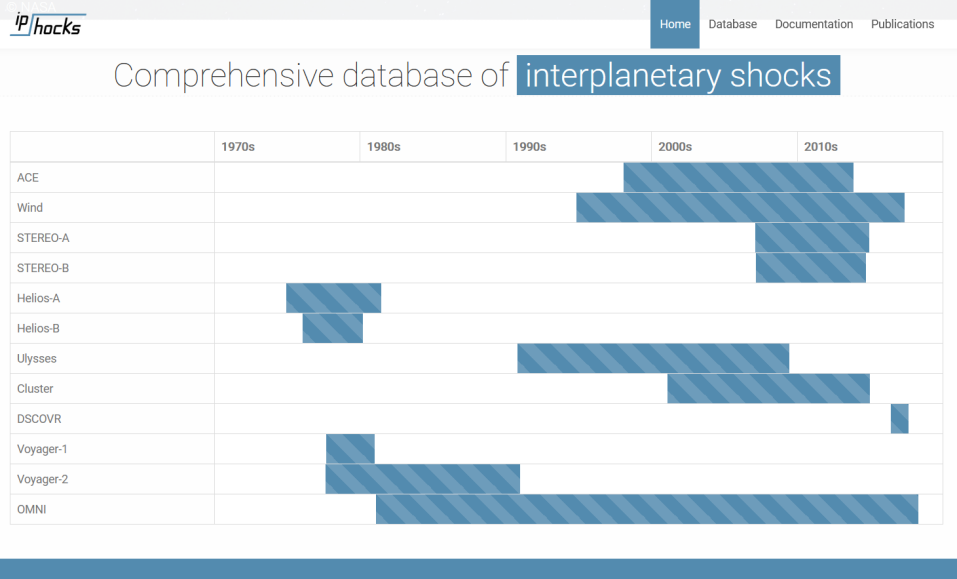
Figure 4.9: Identified shocks detected by the spacecraft in the list

For the event selection I chose the year 2007 for the reason that STEREO$-$A and STEREO$-$B were closer to each other as well as to the Sun-Earth line. Hence, the two events are from this year, particularly on May 07, 2007, and April 23, 2007. In the first event, May 07 of 2007, the selected spacecraft are STEREO$-$A, STEREO$-$B, Wind, and the four cluster satellites: Cluster-1 (C1), Cluster-2 (C2), Cluster-3 (C3), and Cluster-4 (C4), while for the second event, April 23, 2007, the spacecraft are STEREO$-$A and B, ACE, and Wind. After choosing the shock candidates, I downloaded the shock data from NASA’s Coordinated Data Analysis Web (CDAWeb https://cdaweb.gsfc.nasa.gov/). I obtained the STEREO$-$A and B magnetic field observation and the plasma data from the STEREO In-situ Measurements of Particles and CME Transients magnetic field experiment (IMPACT Luhmann et al., 2008) with the time resolution of 100 ms and the STEREO PLAsma and SupraThermal Ion Composition (PLASTIC Galvin et al., 2008) respectively. The magnetic field and the plasma data of the STEREO$-$A and B are in the RTN coordinate system. I obtained the Wind magnetic and plasma data from the Magnetic Field Investigation instrument (MFI Lepping et al., 1995) with a time resolution of 3 sec and The Solar Wind Experiment (SWE Ogilvie et al., 1995) with a time resolution of 1 min respectively. The magnetic field and the plasma data of the Wind are in the Geocentric Solar Ecliptic System (GSE) coordinate system. I obtained the ACE magnetic and plasma data from the ACE Magnetic Field Experiment (MAG Smith et al., 1998) with a time resolution of 1 sec and the Solar Wind Electron Proton Alpha Monitor (SWEPAM McComas et al., 1998) with the time resolution of 64 sec, respectively. The magnetic field and the plasma data are in both the RTN and GSE coordinate systems. I acquired the magnetic data of Cluster satellites from the Cluster Fluxgate Magnetometer (FGM Balogh et al., 1997) with a time resolution of four sec for all the four Cluster satellites, ion data from the Cluster Ion Spectrometry (Reme et al., 1997; CIS) with a time resolution of 4 sec for the Cluster-1 and Cluster-3 satellites, and the spacecraft potential data from Electric Fields and Waves (EFW Gustafsson et al., 1997) with a time resolution of 4 sec for the Cluster-2 and Cluster-4 satellites. All the Cluster data were in the GSE coordinate system.

After obtaining the data, I transformed the coordinate system transformation in such a way that all the coordinate systems are changed to the Heliocentric Earth Ecliptic (HEE) coordinate system. To transform from the RTN and the GSE coordinate systems to the HEE coordinate system, I used Transformation de REpères en Physique Spatiale (TREPS) online tool. The TREPS tool, which is developed by the French Plasma Physics Data Centre (CDPP), the national data center in France for the solar system plasmas, is based on SPICE (Spacecraft, Planet, Instrument, C-matrix, and Events) information system kernels created by NASA/NAIF. Its use is simple, with a 4-step process, which includes importing data, selecting the original coordinate system of the data and a coordinate system to transform, Figure 4.10, choosing how the transformed vector should be exported, and finally, exporting the transformed file (Genot et al., 2018).

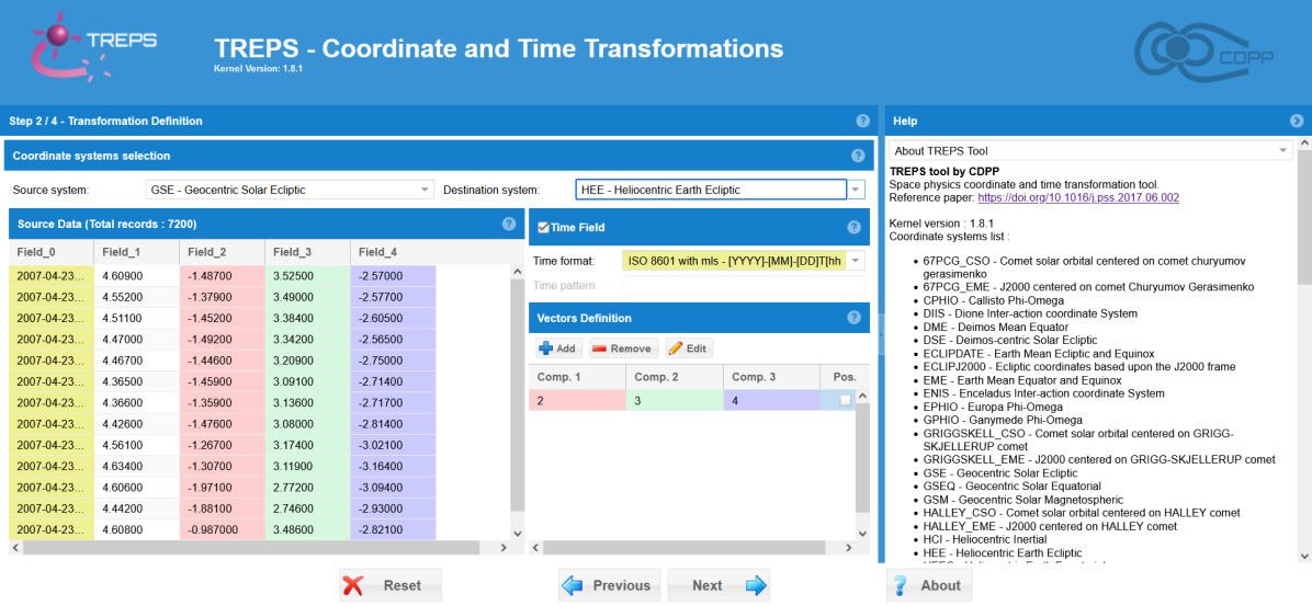
Figure 4.10: TREPS interface, showing a transformation from the GSE to the HEE coordinate system. The green colored column denotes the time field and the other three colored columns denote X, Y, and Z vector components

Chapter 5 Discussion

5.1 Observations

With the visual inspection of the magnetic field and plasma data, I identified jumps in magnetic field B, speed V, density N, and temperature T. Using these variations, I determined the times at which shocks occurred for each spacecraft data set in each event. From the plots, the shocks detected by the spacecraft in each event are believed to be propagation of the same shock due to their timing and the similarities of the magnetic field and plasma data profile with one another. The following case studies of two events are not orderly defined for one another. First, I analyzed the shock event on May 07, 2007, and then the event on April 23, 2007. Hence, the order follows this fashion.

5.1.1 The Event May 07, 2007

On this day, the Wind spacecraft first detected the shock at 07:02:30 UTC. After that, the STEREO$-$A spacecraft detected the shock at 08:11:30 UTC, and then the STEREO$-$B spacecraft detected the shock at 09:42:00 UTC. The four Cluster satellites detect the shock as well. Cluster-1 spacecraft detected the shock at 08:27:55 UTC, and the Cluster-3 spacecraft detected the shock at 08:28:00 UTC. The magnetic field and the plasma plot are shown in Figure 5.1 for the Wind, in Figure 5.2 for the STEREO$-$A, in Figure 5.3 for the STEREO$-$B, in Figure 5.4 for the Cluster-1, in Figure 5.5 for the Cluster-3. There is no indication that Cluster-2 and 4 detected a shock in the shock database list. But the four Cluster satellites are much closer together, so they must have detected the shock. Without plasma data, which is a problem for the Cluster-2 and 4 satellites, a shock cannot be confirmed based solely on the magnetic field data, but there is a way to obtain at least the plasma density parameter using the spacecraft potential, which is a resulting electric potential as the spacecraft travels through the plasma environment, it acquires an electric charge as a result of contact with charged particles. This charging process results in an electrical potential discrepancy between the spacecraft and the plasma around it, a phenomenon referred to as spacecraft potential.

The electron plasma density parameter is obtained by the empirical formula 5.1, as stated in (WHISPER team, 2022) and (Sandhu et al., 2016)

$$N_{e}=200\cdot(-U_{EFW})^{-1.85}$$ (5.1)

So, comparing the magnetic field and the electron plasma density profile, the shock is determined.

The Cluster-2 spacecraft detected the shock at 08:28:10 UTC. Figure 5.6 shows the magnetic field and density plot. The Cluster-4 spacecraft detected the shock at 08:28:10 UTC. Figure 5.7 shows the magnetic field and density plot. Similarly, The electron density parameter is obtained by the empirical formula 5.1.

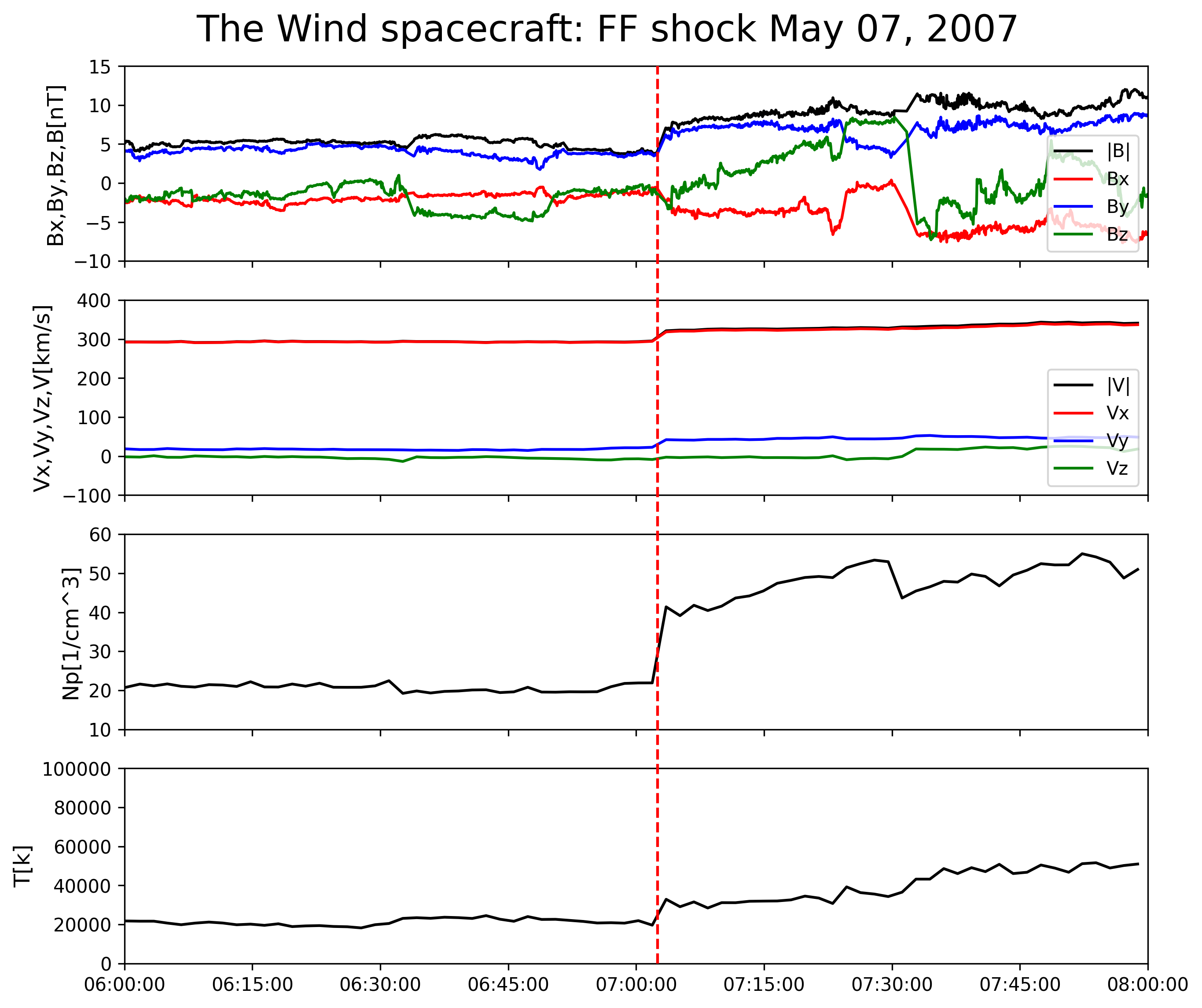
Figure 5.1: The plot of the shock detected by the Wind spacecraft on May 07, 2007, at 07:02:30 UTC. FF stands for the fast forward shock, which means the shock is traveling away from its driver. The panels show from top to bottom, the magnetic field magnitude as well as its components, the total velocity, and its components, density, and temperature. The dashed red line represents the exact shock time. The duration of the plot is two hours.

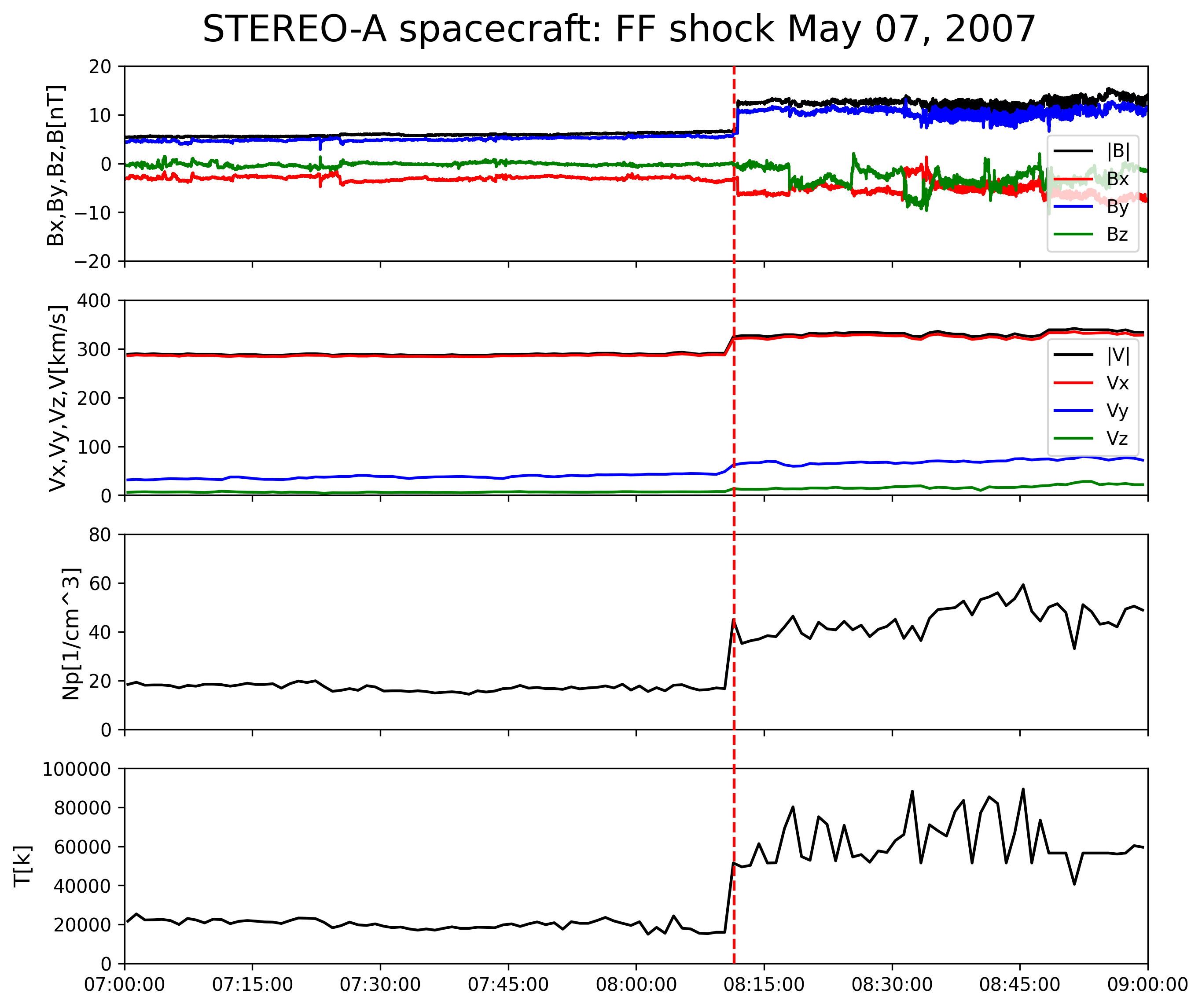
Figure 5.2: The plot of the shock detected by the STEREO$-$A spacecraft on May 07, 2007, at 08:11:30 UTC. The symbols and details of the figures are the same as 5.1. The duration of the plot is two hours.

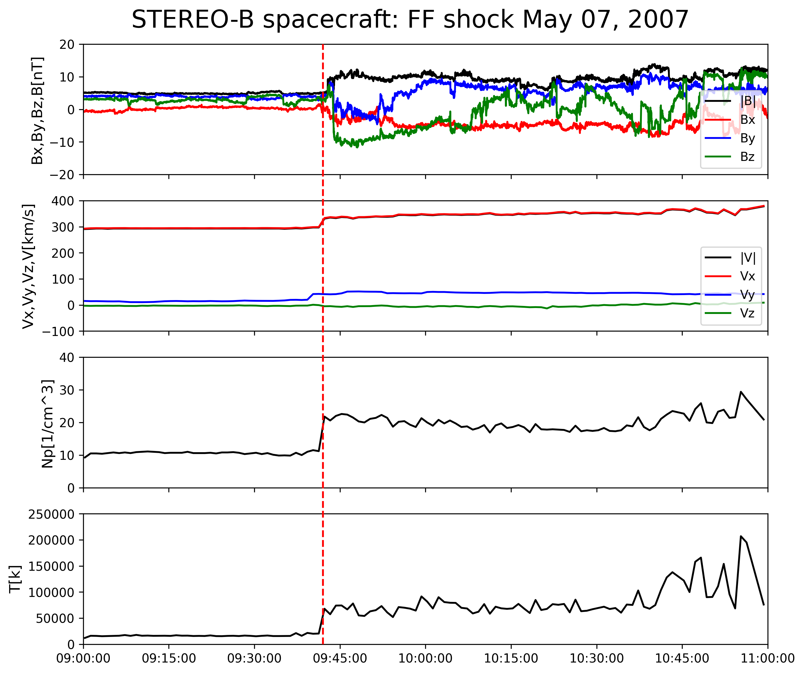
Figure 5.3: The plot of the shock detected by the STEREO$-$B spacecraft on May 07, 2007, at 09:42:00 UTC. The symbols and details of the figures are the same as 5.1. The duration of the plot is two hours.

Figure 5.4: The plot of the shock detected by the Cluster-1 spacecraft on May 07, 2007, at 08:27:55 UTC. The panels show from top to bottom, the magnetic field magnitude as well as its components, the total velocity, and its components, density, and parallel and perpendicular temperatures. The dashed red line represents the exact shock time. The duration of the plot is two hours.

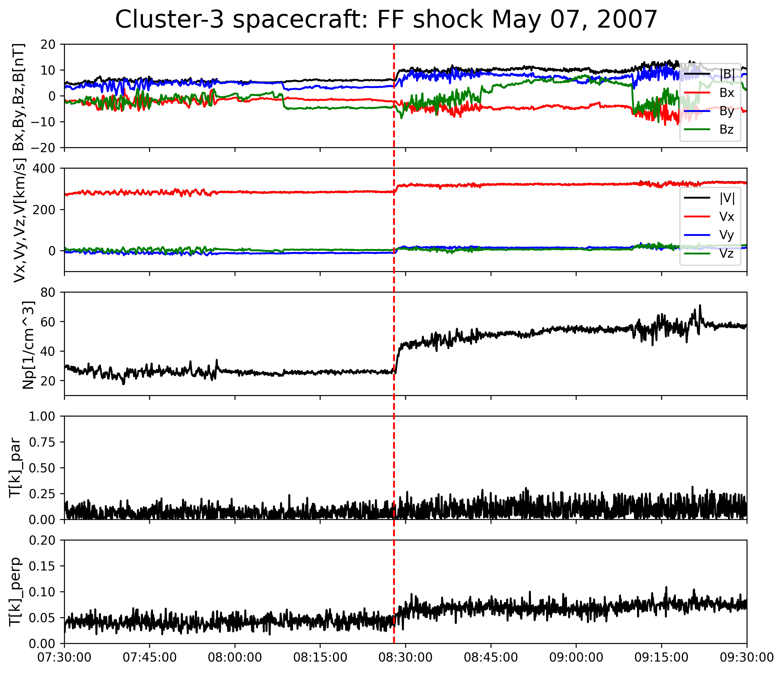
Figure 5.5: The plot of the shock detected by the Cluster-3 spacecraft on May 07, 2007, at 08:28:00 UTC. The symbols and details of the figures are the same as 5.4. The duration of the plot is two hours.

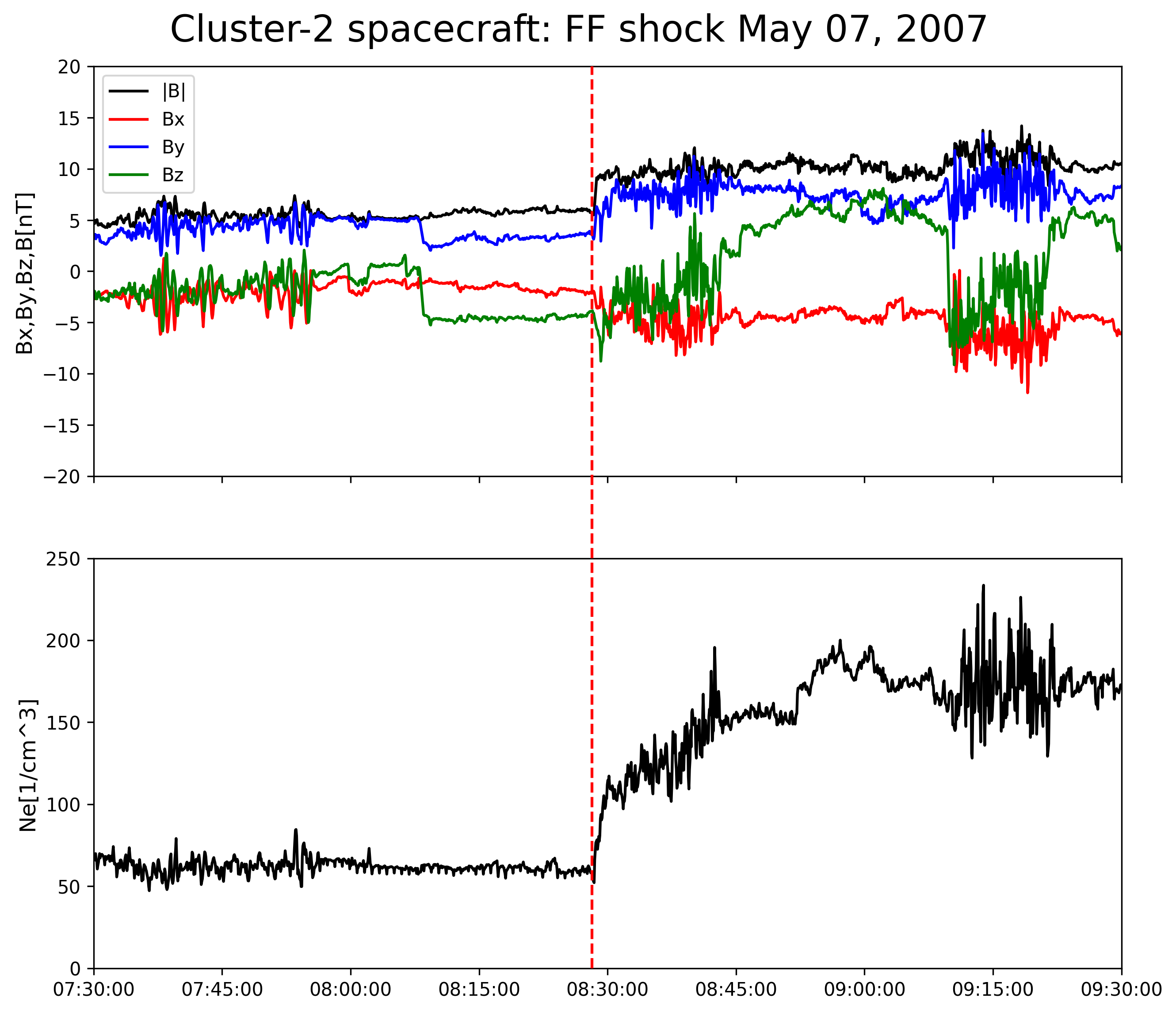
Figure 5.6: The plot of the shock detected by the Cluster-2 spacecraft on May 07, 2007, at 08:28:10 UTC. The panels show from top to bottom, the magnetic field magnitude as well as its components, and the obtained electron density from the spacecraft potential. The dashed red line represents the exact shock time. The duration of the plot is two hours.

Figure 5.7: The plot of the shock detected by the Cluster-4 spacecraft on May 07, 2007, at 08:28:10 UTC. The symbols and details of the figures are the same as 5.6. The duration of the plot is two hours.

5.1.2 The Event April 23, 2007

In this specific event STEREO$-$A spacecraft detected a shock first at 06:53:35 UTC, then the ACE spacecraft detected the shock at 08:57:00 UTC, and the Wind spacecraft detected the shock at 09:12:00 UTC. The magnetic field and the plasma data are shown in Figure 5.8 for the STEREO$-$A, in Figure 5.9 for the ACE, and in Figure 5.10 for the Wind.

Since STEREO$-$A and B have identical instruments, STEREO$-$B must have detected the shock on that day even though there is no detected IP shock for STEREO$-$B in the shock lists database mentioned above. So, by using the average solar wind speed, 400 km/s, we concluded that the shock detection time for STEREO$-$B should be around 13:00 to 15:00. Considering this, a could-be shock signature from STEREO$-$B is found around 13:21:30 even though it is a faint signature. The magnetic field and the plasma plot are shown in Figure 5.11

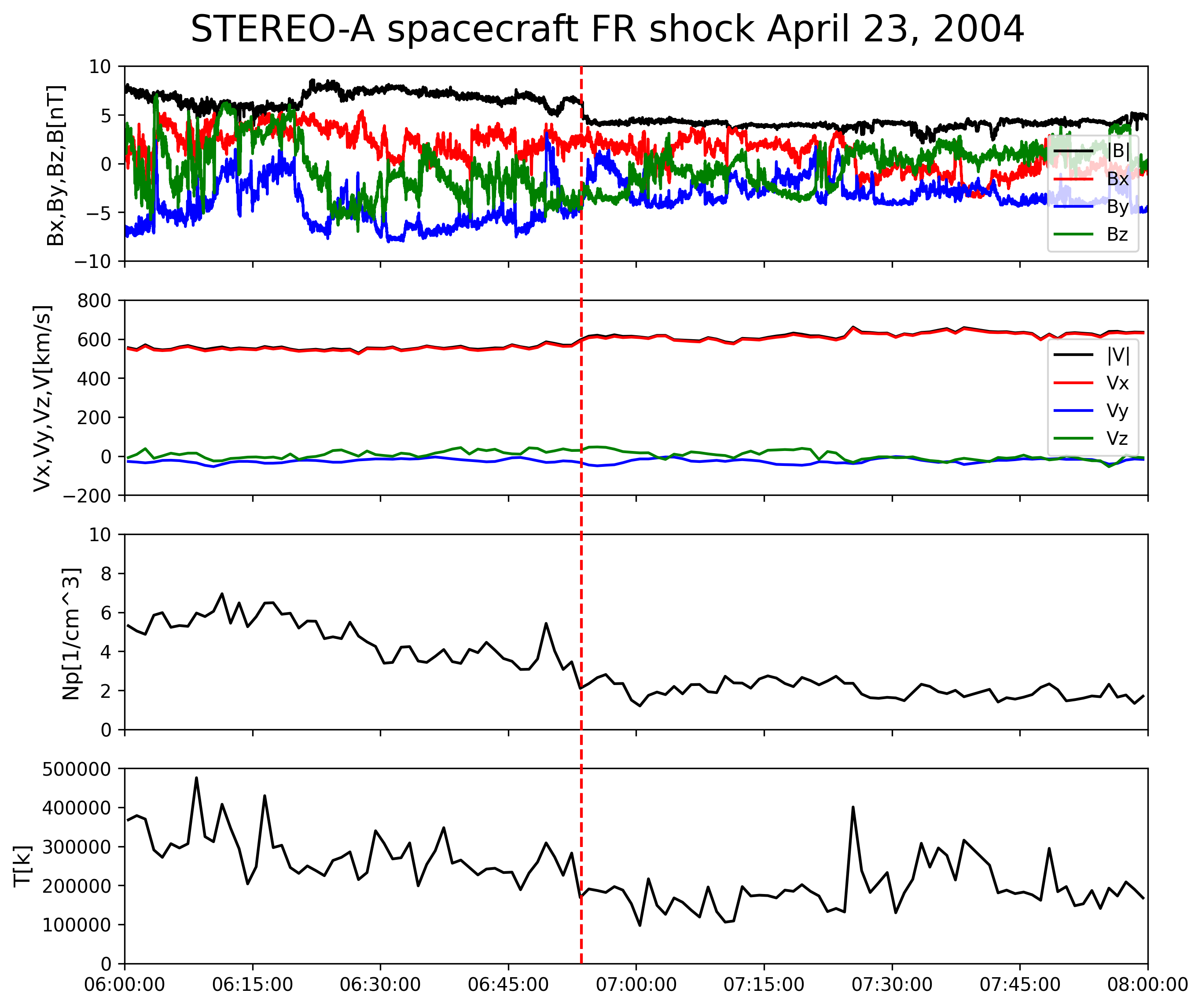
Figure 5.8: The plot of the shock detected by the STEREO$-$A spacecraft on April 23, 2007, at 06:53:35 UTC. FR stands for the fast reverse shock, which means the shock is moving toward its driver. The panels show from top to bottom, the magnetic field magnitude as well as its components, the total velocity and its components, density, and temperature. The dashed red line represents the exact shock time. The duration of the plot is two hours

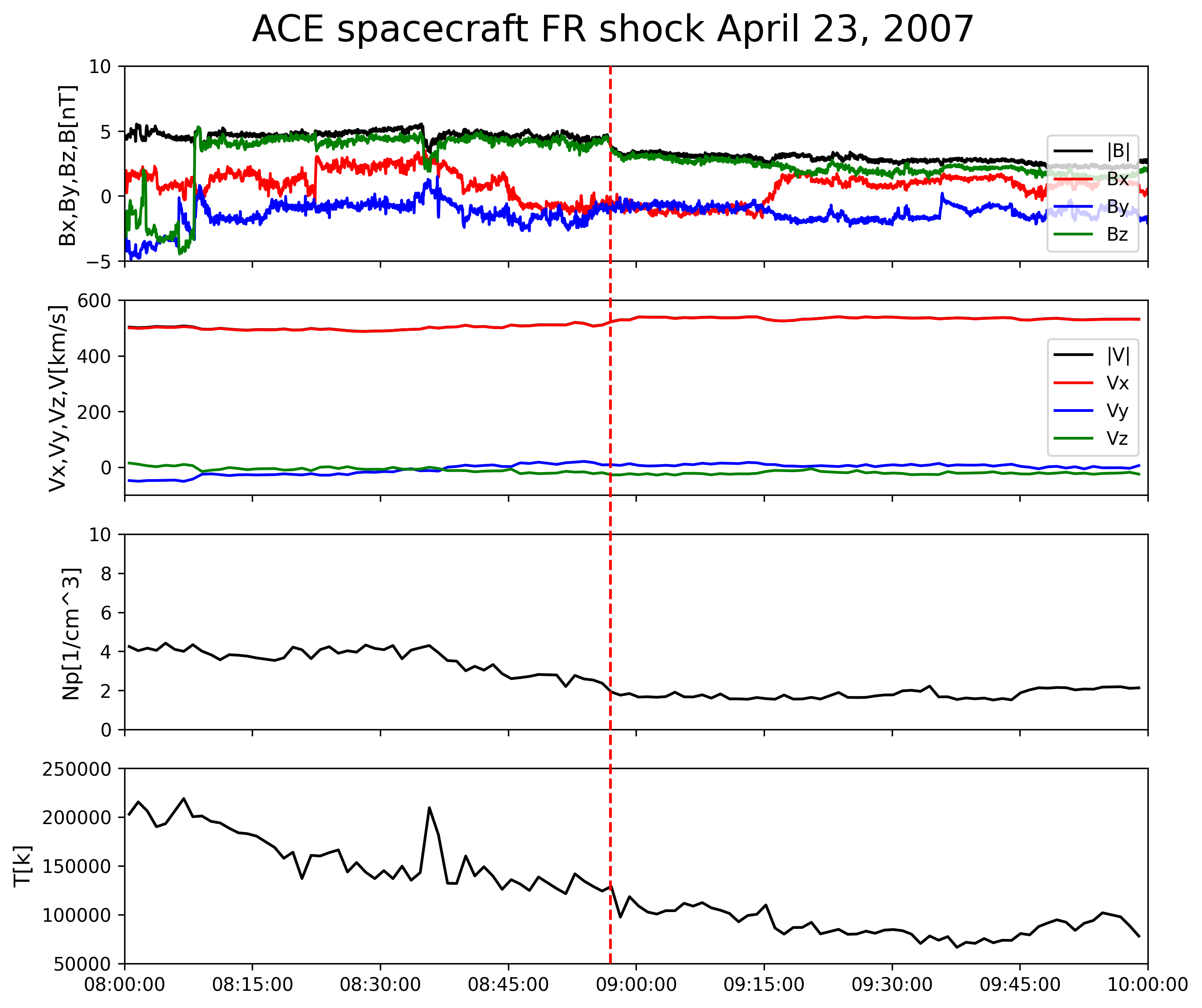
Figure 5.9: The plot of the shock detected by the ACE spacecraft on April 23, 2007, at 08:57:00 UTC. The symbols and details of the figures are the same as 5.8. The duration of the plot is two hours.

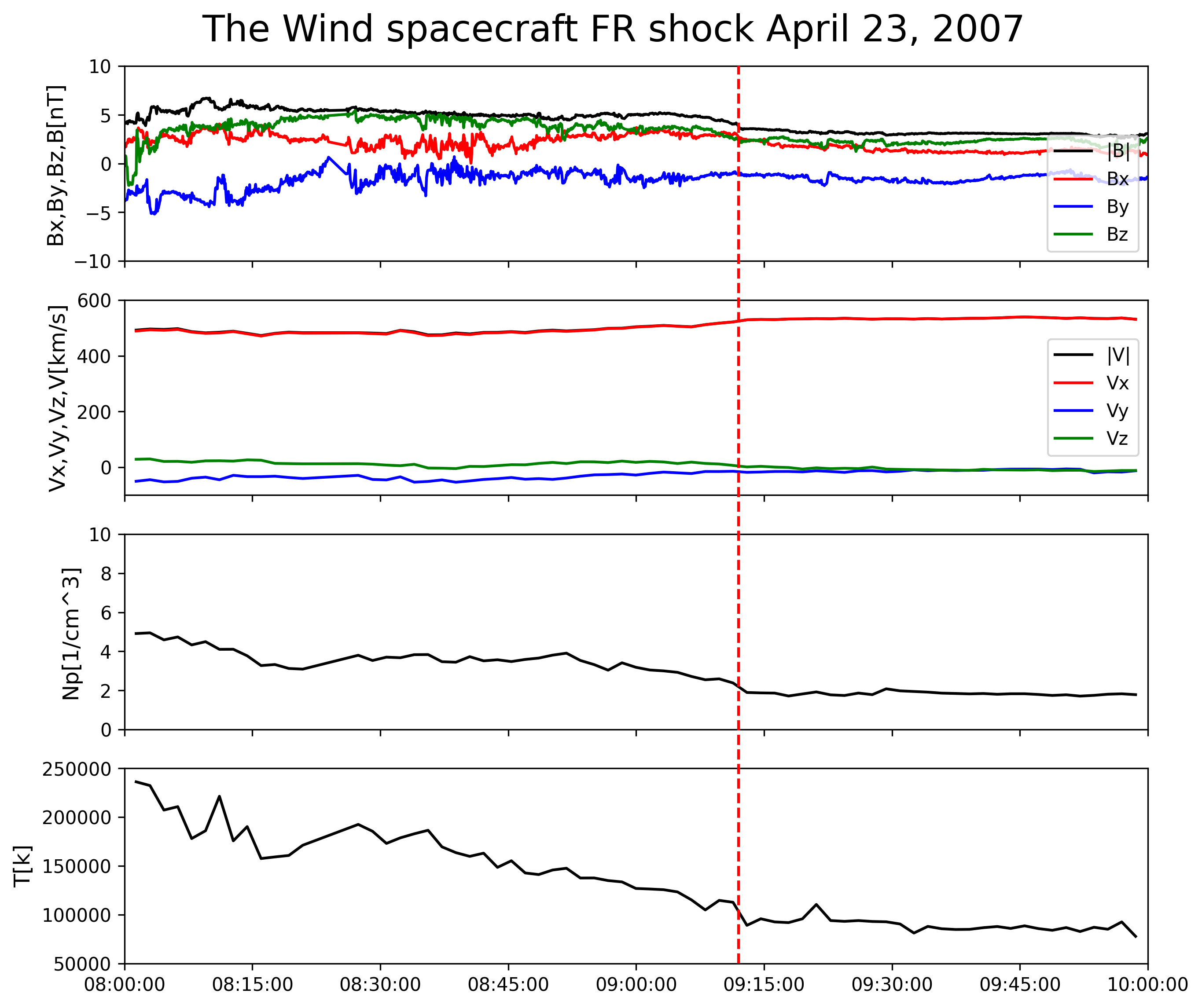
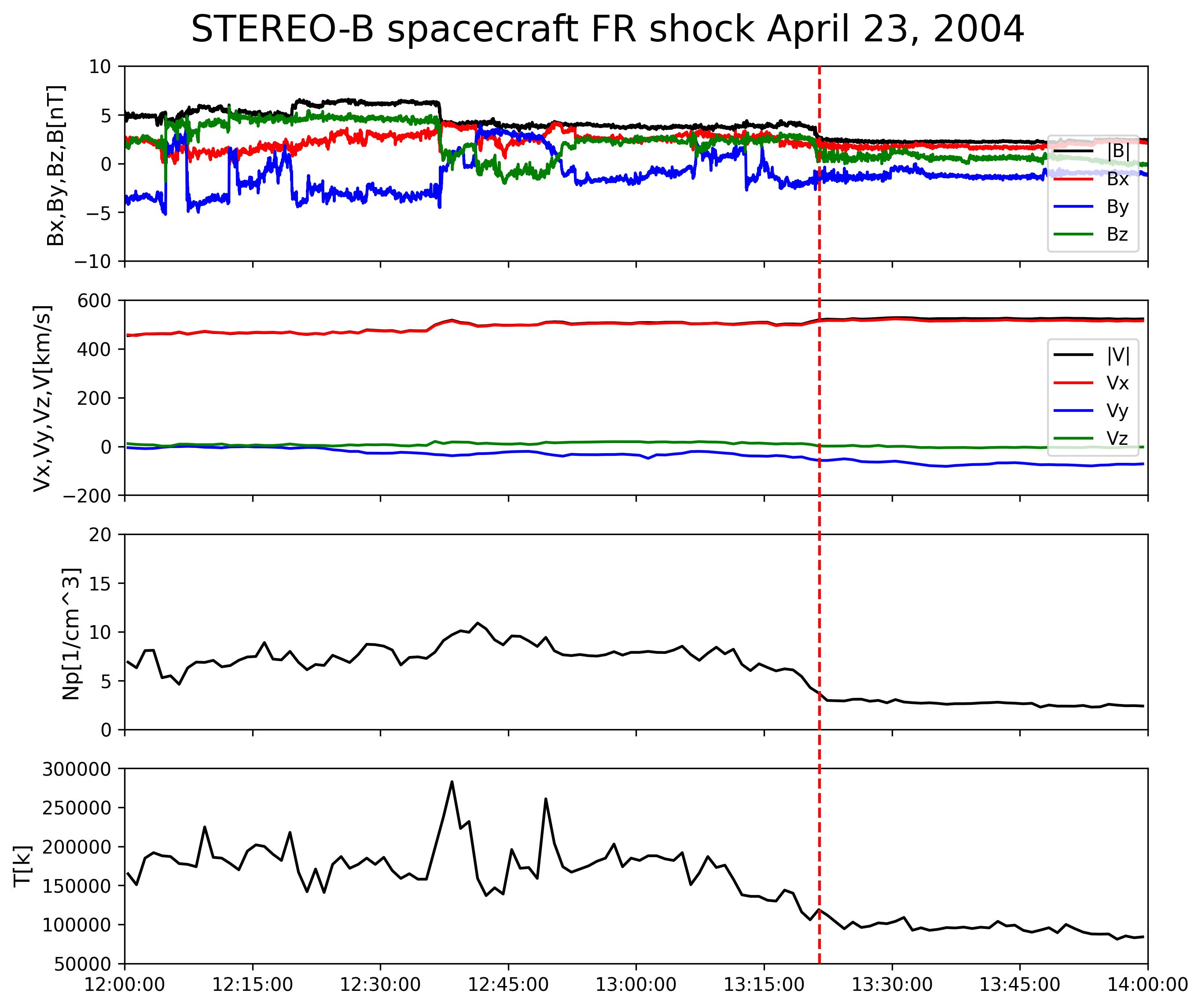
Figure 5.10: The plot of the shock detected by the Wind spacecraft on April 23, 2007, at 09:12:00 UTC. The symbols and details of the figures are the same as 5.8. The duration of the plot is two hours.

Figure 5.11: The plot of the shock detected by the Wind spacecraft on April 23, 2007, around 13:21:30 UTC. The symbols and details of the figures are the same as 5.8. The duration of the plot is two hours.

5.2 Implementation of the methods on the events

5.2.1 The Event May 07, 2007

Here I list all magnetic field observations of the spacecraft for the event and apply the minimum variance analysis (MVA) and the magnetic coplanarity (CP) methods on them. The upstream and downstream time intervals that most agree between the minimum variance analysis (MVA) and the magnetic coplanarity methods (CP) for all the spacecraft are shown in Table 5.1, and their corresponding Figures are 5.12 for the Wind, 5.13 for the STEREO$-$A, 5.14 for the STEREO$-$B, 5.15 for the Cluster-1, 5.16 for the Cluster-3, 5.17 for the Cluster-2, and 5.18 for the Cluster-4. Table 5.1 also shows the ratio between the smallest eigenvalue $\lambda_{3}$ and the intermediate eigenvalue $\lambda_{2}$ as well as the angle between the MVA normal and CP normals in the determined upstream and downstream time intervals for each spacecraft.

Implementation of the methods on the event May 07, 2007

Spacecraft	$\Delta t_{up}$	$\Delta t_{down}$	$\lambda_{2}/\lambda_{3}$	$\Delta\theta_{MVA-CP}$
Wind	(06:59:00 - 07:01:47)	(07:03:50 - 07:05:50)	14.82	$0.38^{\circ}$
STEREO$-$A	(08:08:00 - 08:10:05)	(08:12:30 - 08:13:50)	3.16	$0.375^{\circ}$
STEREO$-$B	(09:37:00 - 09:40:35)	(09:42:57 - 09:43:38)	9.51	$1.1^{\circ}$
Cluster-1	(08:26:10 - 08:27:00)	(08:28:00 - 08:29:00)	167.9	$0.21^{\circ}$
Cluster-3	(08:26:30 - 08:27:10)	(08:29:00 - 08:29:47)	22.43	$1.92^{\circ}$
Cluster-2	(08:26:56 - 08:27:40)	(08:28:32 - 08:29:37)	91.56	$0.1^{\circ}$
Cluster-4	(08:26:25 - 08:27:10)	(08:28:45 - 08:29:40)	238.63	$2.49^{\circ}$

Table 5.1: Here, $\Delta t_{up}$ denotes the defined upstream and $\Delta t_{down}$ denotes the defined downstream time intervals with MVA and CP analysis methods. $\lambda_{2}/\lambda_{3}$ indicates the ratio between the intermediate eigenvalue $\lambda_{2}$ and the smallest eigenvalue $\lambda_{3}$, and $\Delta\theta_{MVA-CP}$ is the angle between the MVA and CP normals.

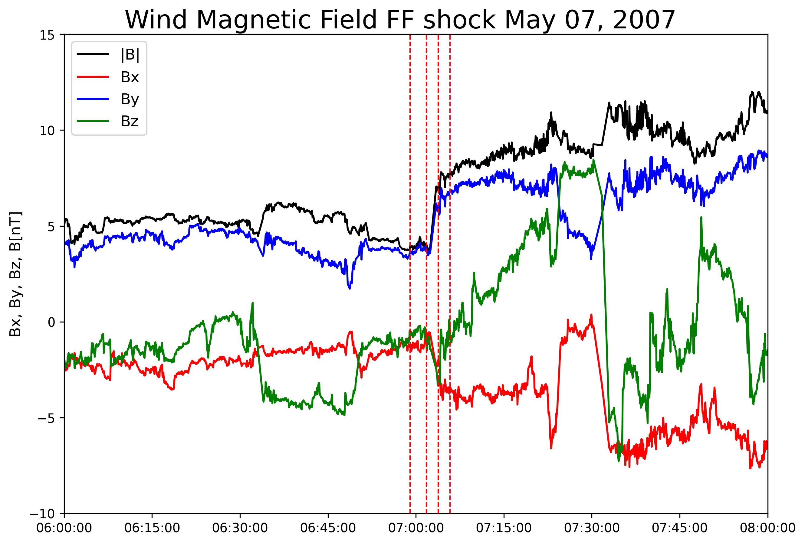
Figure 5.12: The Wind magnetic field measurements. The upstream $\Delta t_{up}$ is between (06:59:00 - 07:01:47), and the downstream $\Delta t_{down}$ is between (07:03:50 - 07:05:50). FF stands for the fast forward shock, which means the shock is traveling away from its driver. The chosen intervals of the upstream and downstream magnetic field. The red dashed lines each represent the upstream starting time and ending time and the downstream starting time and ending time, respectively

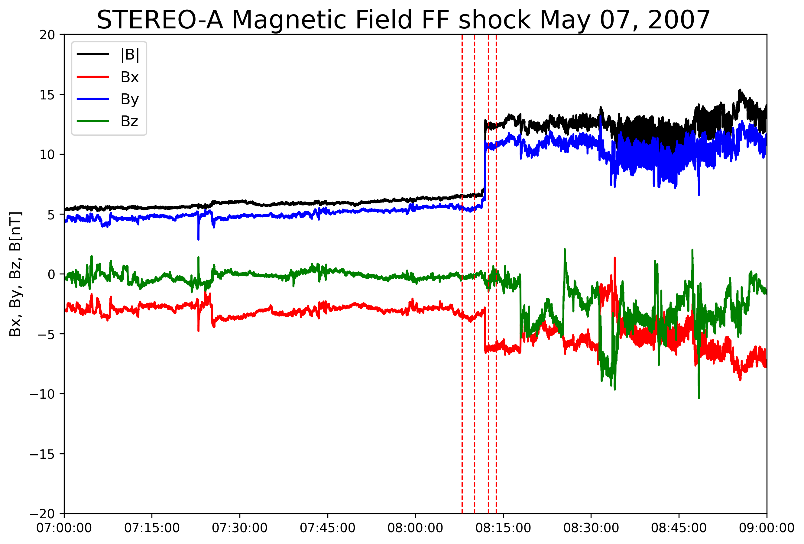
Figure 5.13: The STEREO$-$A magnetic field measurements. The upstream $\Delta t_{up}$ is between (08:08:00 - 08:10:05), and the downstream $\Delta t_{down}$ is between (08:12:30 - 08:13:50). The symbols and details of the figures are the same as 5.12

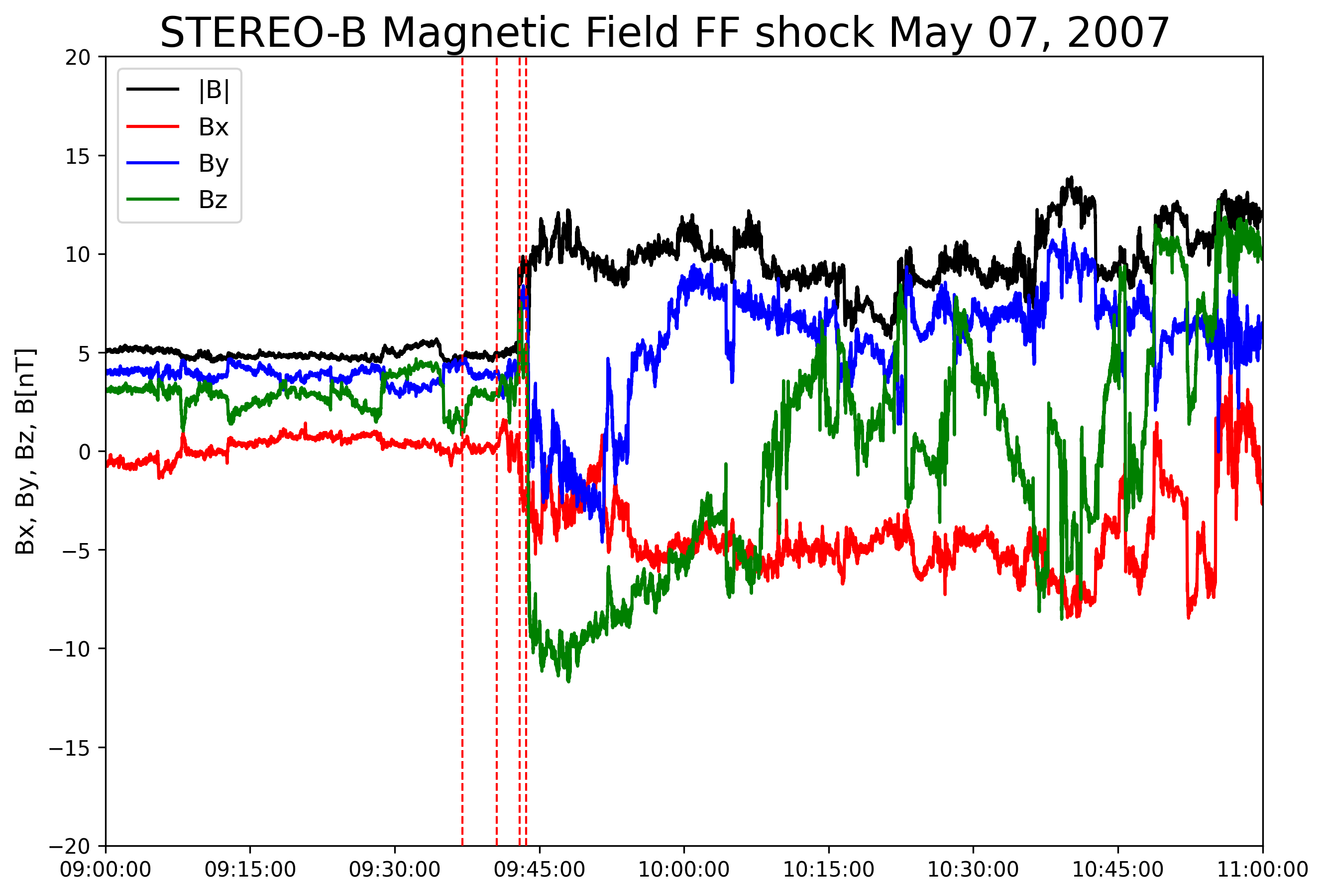
Figure 5.14: The STEREO$-$B magnetic field measurements. The upstream $\Delta t_{up}$ is between (09:37:00 - 09:40:35), and the downstream $\Delta t_{down}$ is between (09:42:57 - 09:43:38). The symbols and details of the figures are the same as 5.12

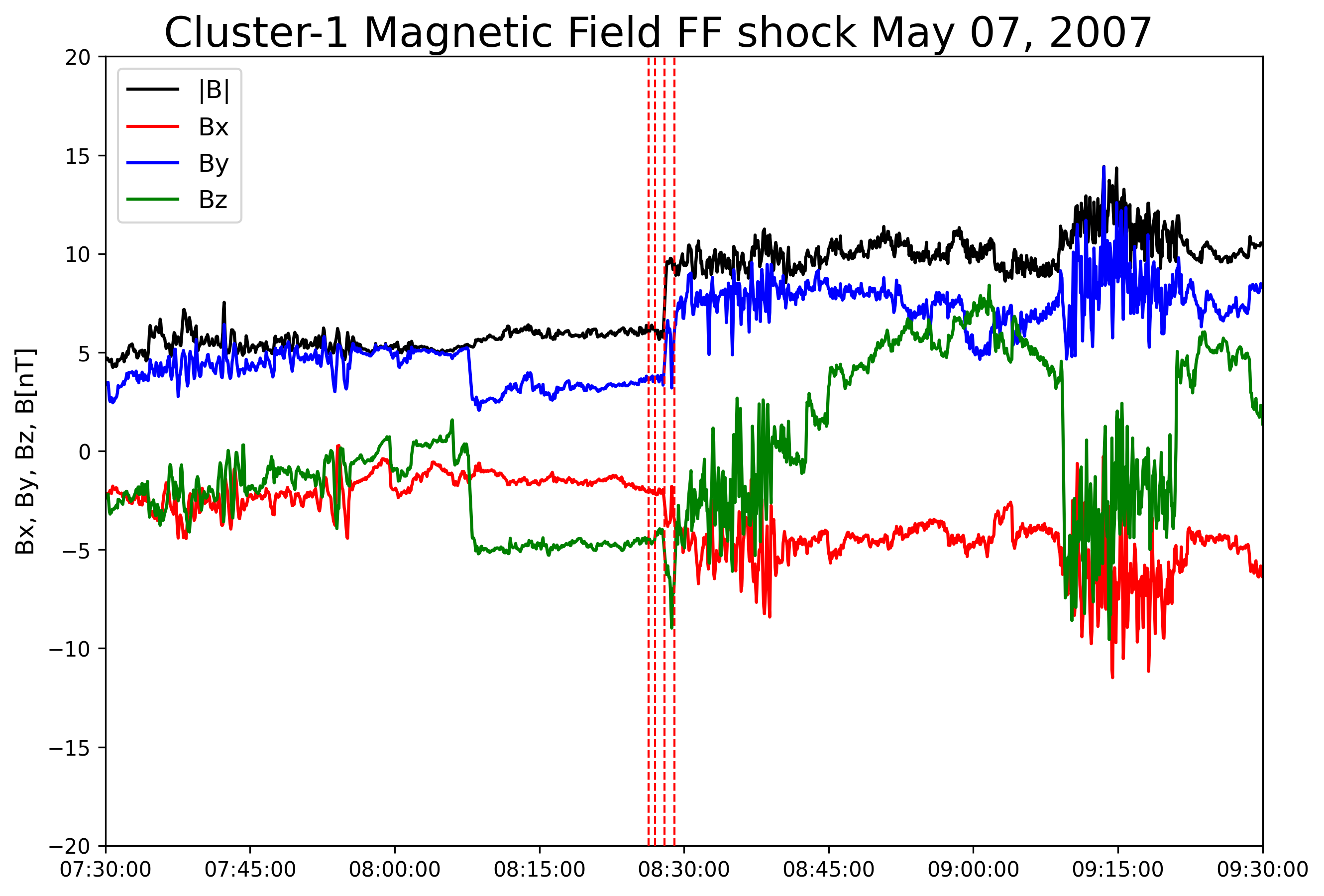
Figure 5.15: The Cluster-1 B magnetic field measurements. The upstream $\Delta t_{up}$ is between (08:26:10 - 08:27:00), and the downstream $\Delta t_{down}$ is between (08:28:00 - 08:29:00). The symbols and details of the figures are the same as 5.12

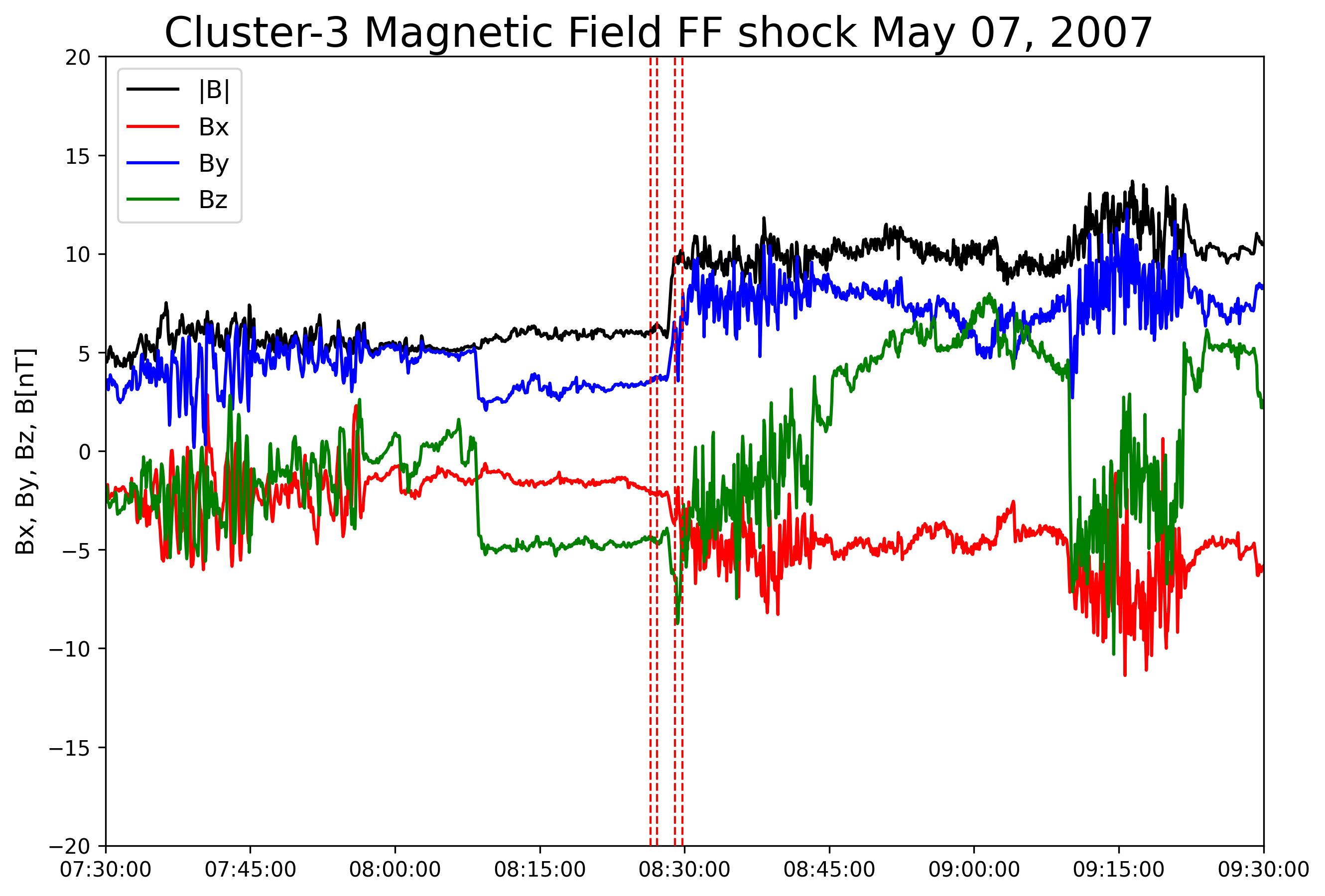
Figure 5.16: The Cluster-3 B magnetic field measurements. The upstream $\Delta t_{up}$ is between (08:26:30 - 08:27:10), and the downstream $\Delta t_{down}$ is between (08:29:00 - 08:29:47). The symbols and details of the figures are the same as 5.12

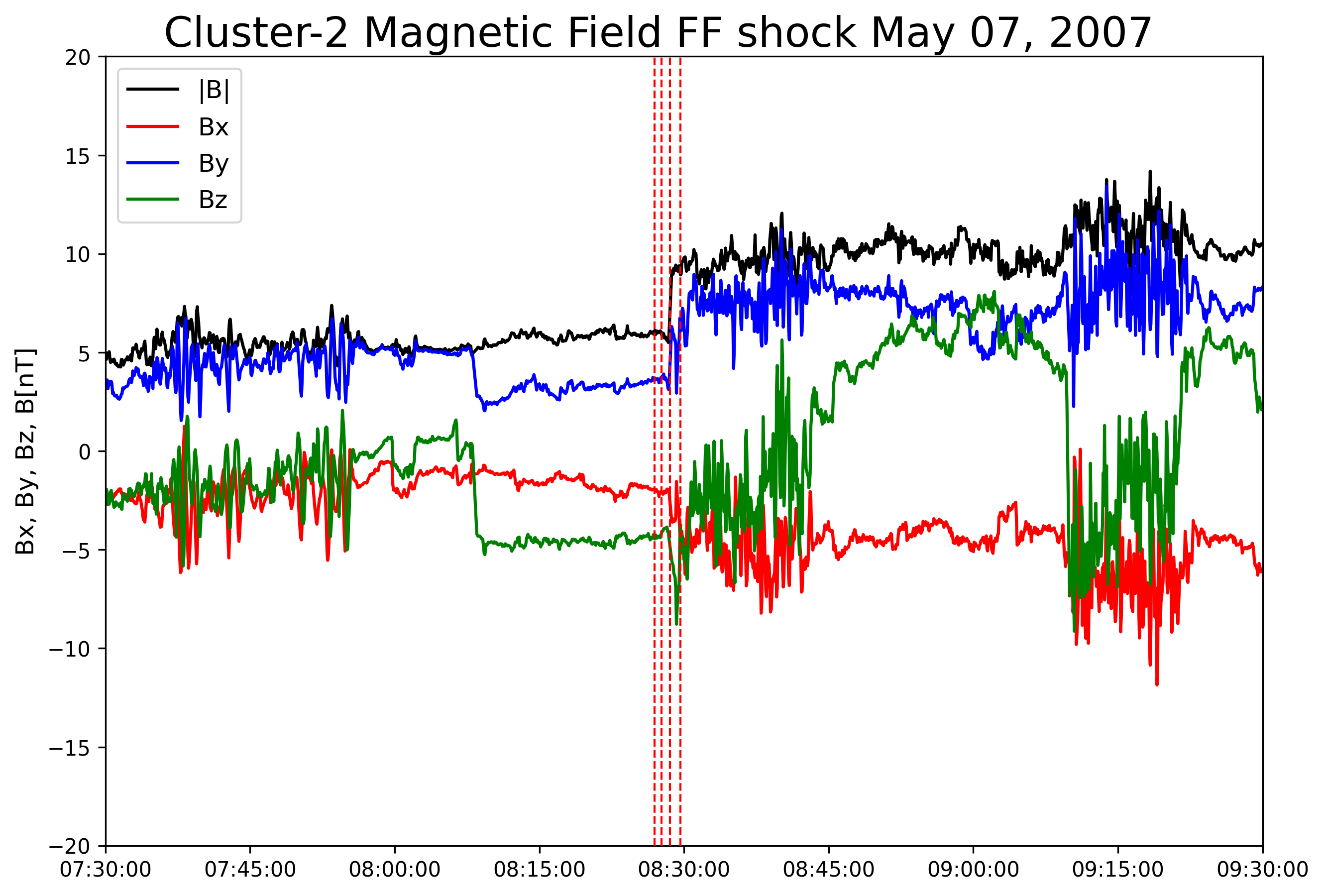
Figure 5.17: The Cluster-2 B magnetic field measurements. The upstream $\Delta t_{up}$ is between (08:26:56 - 08:27:40), and the downstream $\Delta t_{down}$ is between (08:28:32 - 08:29:37). The symbols and details of the figures are the same as 5.12

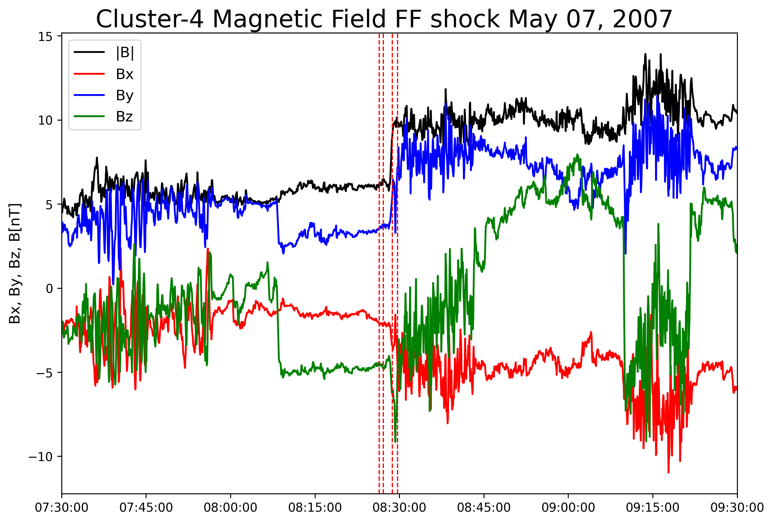
Figure 5.18: The Cluster-4 B magnetic field measurements. The upstream $\Delta t_{up}$ is between (08:26:25 - 08:27:10), and the downstream $\Delta t_{down}$ is between (08:28:45 - 08:29:40). The symbols and details of the figures are the same as 5.12

5.2.2 Analysis of the Event May 07, 2007

The accepted upstream and downstream time intervals are highly accurate considering the angle difference between the two methods is minimal and the eigenvalue criteria are sufficient for each spacecraft data. Using the determined time intervals, the calculations of the ratio between the upstream and downstream magnetic fields, densities, and temperatures as well as the bulk speed, and shock $\theta_{Bn}$ angle are made. These parameters, the minimum variance analysis normal, and the magnetic coplanarity normals are shown in Table 5.2, where the solar wind bulk speed and the downstream to upstream ratios for the shock criteria are fulfilled as stated in 4.14 and 4.15, and the results of the additional parameters calculations as stated in 4.2.4 are shown in Table 5.4.

Spacecraft $B_{d}/B_{u}$ $N_{d}/N_{u}$ $T_{d}/T_{u}$ $\Delta V$ $\theta_{Bn}$ Spacecraft MVA Coplanarity $\Delta\theta_{MVA-CP}$ Wind $1.86\pm 0.10$ $1.78$* $1.33$* $29.6$* 70.80 Wind [-0.763, -0.63, -0.144] [-0.763, -0.629, -0.15] 0.37 STEREO$-$A $1.89\pm 0.02$ $2.18\pm 0.9$ $3.21\pm 2.4$ $36\pm 6$ 81.83 STEREO$-$A [0.889, 0.436, 0.137] [0.888, 0.436, 0.144] 0.38 STEREO$-$B $1.90\pm 0.07$ $1.90\pm 0.6$ $2.90\pm 6$ $40.25\pm 11$ 59.45 STEREO$-$B [-0.855 -0.511 -0.087] [-0.864 -0.497 -0.077] 1.10 Cluster 1 $1.53\pm 0.04$ $1.63\pm 0.09$ $1.10\pm 1.3_{par}$ $31.2\pm 3.1$ 86.62 Cluster-1 [0.846 0.532 -0.029] [-0.847 -0.530 -0.032] 0.21 $1.40\pm 0.32_{perp}$ Cluster 3 $1.57\pm 0.05$ $1.69\pm 0.08$ $1.20\pm 1.5_{par}$ $30.5\pm 2.8$ 89.74 Cluster-3 [0.753 0.639 0.153] [-0.763 -0.633 -0.121] 1.92 $1.40\pm 0.40_{perp}$ Cluster 2 $1.53\pm 0.03$ $1.42\pm 0.18$ NaN NaN 88.19 Cluster-2 [0.838 0.545 0.012] [-0.838 -0.544 -0.013] 0.10 Cluster 4 $1.57\pm 0.05$ $1.49\pm 0.19$ NaN NaN 86.55 Cluster-4 [0.858 0.506 -0.080] [0.838 0.533 0.108] 2.49

Table 5.2: Resulting core parameters of studying the data of the Wind, STEREO$-$A, STEREO$-$B, Cluster-1, Cluster-3, Cluster-2, and Cluster-4 spacecraft. Here $\theta_{Bn}$ is the shock $\theta$ angle. The values with the asterisk (*) symbol indicate the parameters with indefinite uncertainties because the determined intervals of the upstream and downstream magnetic fields are smaller than the resolution of the plasma data. Due to the CIS experiment is not operational for Cluster-2, and the HIA instrument being switched off for Cluster-4 spacecraft, the plasma parameters are not available for these satellites.

Table 5.3: (Continued) Resulting core parameters of studying the data of the Wind, STEREO$-$A, STEREO$-$B, Cluster-1, Cluster-3, Cluster-2, and Cluster-4 spacecraft. $\theta_{MVA-CP}$ is the angle difference between the minimum variance normal vectors and the magnetic coplanarity normal vectors.

Spacecraft $V_{sh}$ km/s $C^{up}_{s}$ km/s $V^{up}_{A}$ km/s $C^{up}_{ms}$ km/s Spacecraft Plasma $\beta_{up}$ Alfvén Mach Magnetosonic Mach Wind 313.60 $47.20\pm 1.60$ $18.70\pm 6.08$ $50.78\pm 2.7$ Wind $7.6\pm 4.9$ $4.14\pm 1.72$ $1.50\pm 0.40$ STEREO$-$A 352.41 $46.27\pm 3.30$ $34.89\pm 15$ $57.95\pm 9.41$ STEREO$-$A $2.11\pm 1.8$ $2.19\pm 1.12$ $1.32\pm 0.42$ STEREO$-$B 354.91 $46.89\pm 5.85$ $31.95\pm 7.33$ $56.74\pm 6.35$ STEREO$-$B $2.58\pm 1.34$ $2.76\pm 1.07$ $1.55\pm 0.52$ Cluster 1 342.02 $43.88\pm 3.09$ $25.59\pm 7.70$ $51.31\pm 3.99$ Cluster-1 $3.26\pm 1.89$ $3.84\pm 1.40$ $1.99\pm 0.46$ Cluster 3 308.11 $43.88\pm 2.63$ $26.80\pm 7.64$ $51.42\pm 3.98$ Cluster-3 $3.21\pm 1.83$ $3.72\pm 1.35$ $1.93\pm 0.46$

Table 5.4: Resulting additional parameters of studying the data of the three spacecraft. $V_{sh}$ is the shock speed, $C^{up}_{s}$ is the upstream sound speed, $V^{up}_{A}$ is the upstream Alfvén speed and $C^{up}_{ms}$ is the upstream magnetosonic speed.

Table 5.5: (Continued) Resulting additional parameters of studying the data of the three spacecraft. Plasma $\beta_{up}$, Alfvén Mach, and Magnetosonic Mach are shown

Using the results, the 2D sketches of the IP shocks that were detected by the spacecraft are shown in Figure 5.19(a), 5.19(b), 5.19(c). In these 2D sketches, the shock propagation and normal vector orientation are shown in a temporal development manner. Since 4 Cluster satellites are relatively close to one another, their averaged position as well as normal vectors are shown in the general 2D and 3D sketches. For explicitly showing normal vector directions and positions of all 4 Clusters satellites, it is suitable to change their coordinates and normal vectors into a GSE coordinate system with the positions in the earth radii (RE) unit, see Figure 5.20.

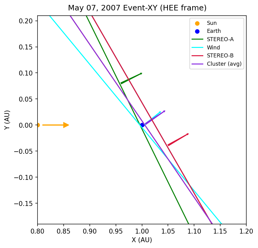
(a)

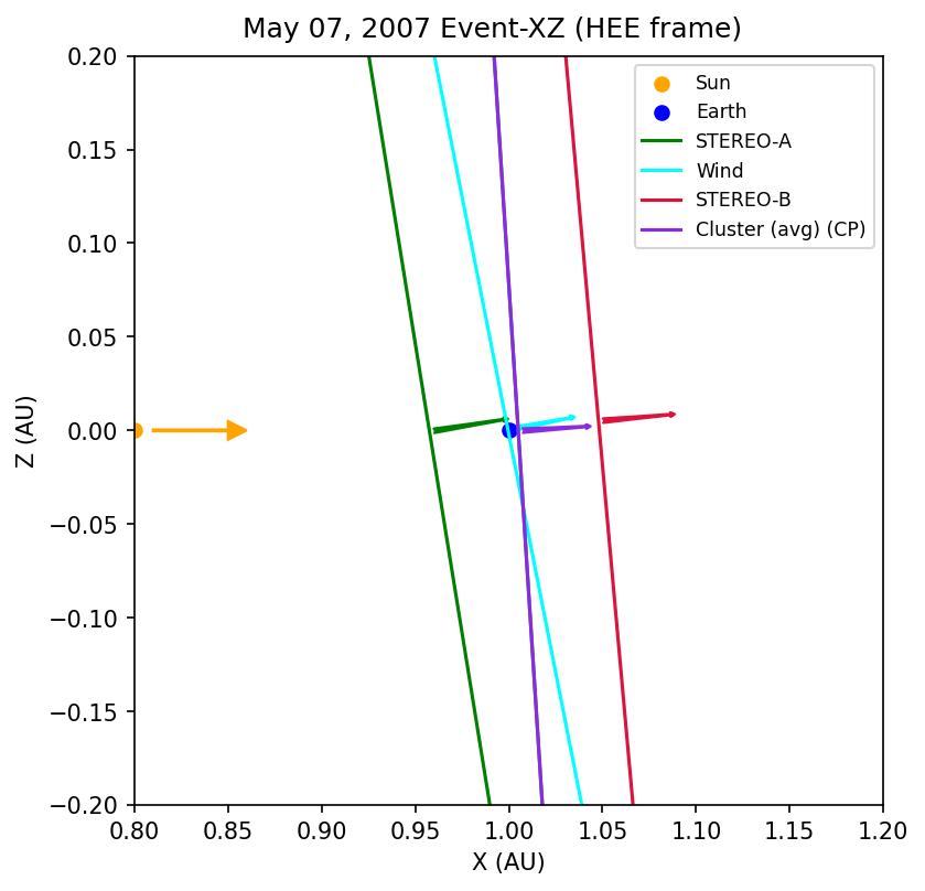
(b)

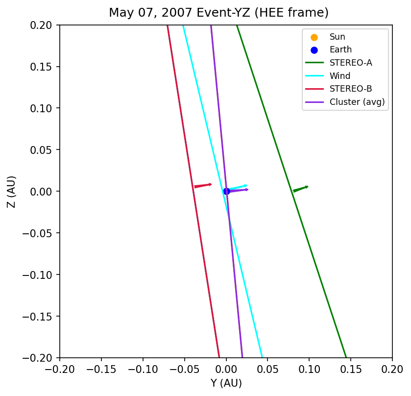
(c)

Figure 5.19: 2D XY, XZ, and YZ sketches of the propagation of the IP shock through spacecraft– Wind, STEREO$-$A and B, and average position of 4 Cluster satellites. The orange arrow represents the Sun-Earth line direction. The arrows on spacecraft positions indicate the normal vector direction and the lines perpendicular to the normal vectors indicate the shock surface orientations. The sizes of the lines are arbitrary. The shock orientations for the 4 Cluster satellites are averaged

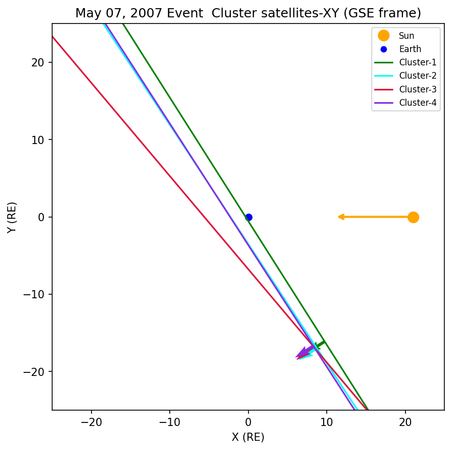
(a)

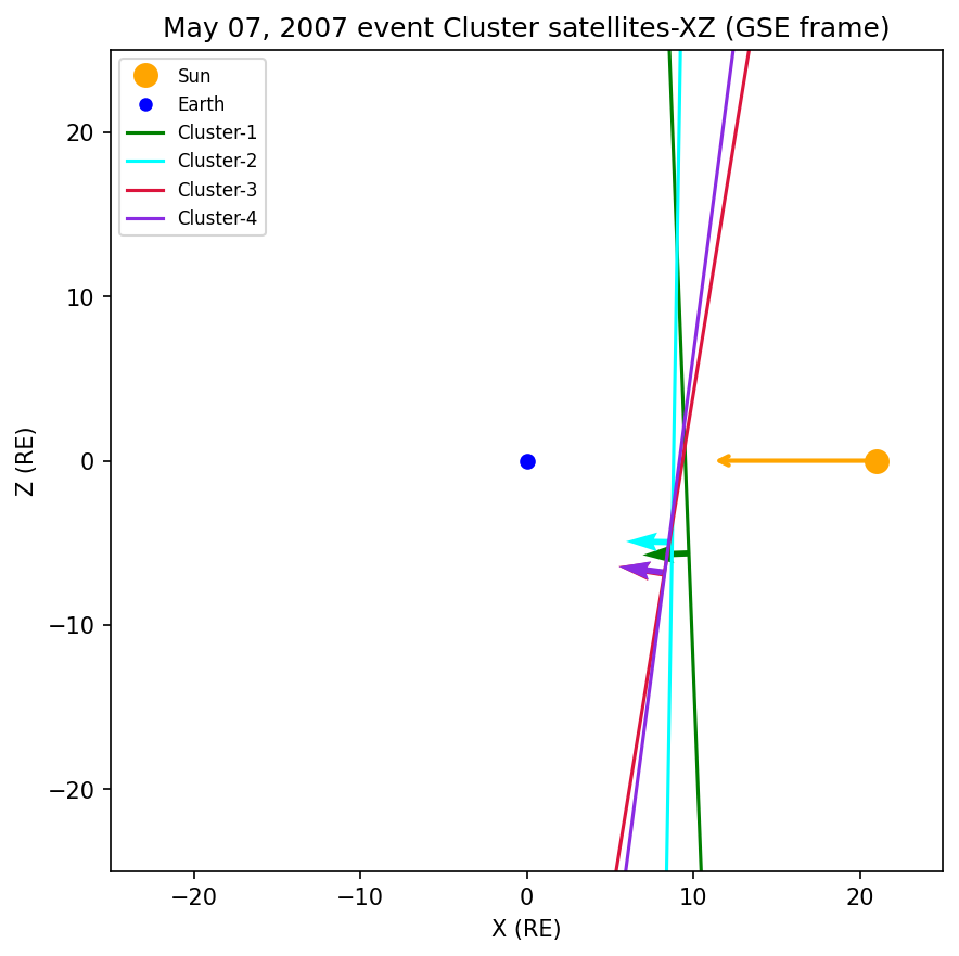
(b)

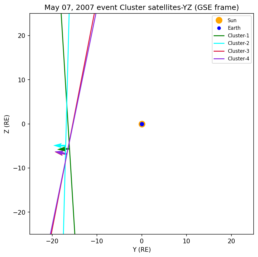
(c)

Figure 5.20: 2D sketch of the propagation of the IP shock through 4 Cluster satellites – SC1, SC2, SC3, and SC4. The orange arrow represents the Sun-Earth line direction. The arrows on spacecraft positions indicate the normal vector direction and the lines perpendicular to the normal vectors indicate the shock surface orientations. The sizes of the lines are arbitrary.

5.2.3 Discussion of the Event May 07, 2007

The 3D sketch is shown in 5.22, and in the 3D sketch, the STEREO$-$A, and B, and averaged Clusters positions are time-shifted to the Wind’s position to see the overall shape of this IP shock. From the 3D sketch, the overall shape of the IP shock is a planner and can be fitted with a plane. The IP shock fitted plane is tilted $56.42^{\circ}$ with respect to the Sun-Earth line according to Figure 5.22(c). The tilt appears to be almost the same degree as the Parker spiral impacting the Earth from the dawn side. Hence, it is the reason why the Wind detected the shock first even though STEREO$-$A’s position is relatively closer to the Sun’s direction. This period, 2007, was during the solar minimum phase, and stream interaction region (SIR) or co-rotating stream interactions (CIR) were dominant (Opitz et al., 2014), and this further proves the result, see Figure 5.21. Furthermore, to see a correlation between fast-forward shock and geomagnetic activity, I determined the Kp-index of May 07, 2007, as shown in Figure 5.23. It appears that this forward shock-leading event disturbed the magnetosphere, causing a G1-minor geomagnetic storm with the Kp index peaking around 15:00 UTC. The geomagnetic substorm happened about 6 hours after the detection of the shock by the STEREO$-$B spacecraft.

Figure 5.21: The Figure presents data from STEREO$-$A between February 1, 2007, and June 1, 2007. It illustrates the PLASTIC bulk velocity, the SWEA proxy for electron density, the overall magnetic field strength as measured by MAG, and the SEPT ion intensity ranging from 110 keV to 2200 keV. Periods featuring well-established Co-rotating Interaction Regions (CIRs) with noticeable boosts in ion energy are highlighted with grey shading. (Figure is from Opitz et al., 2014; Figure 2)

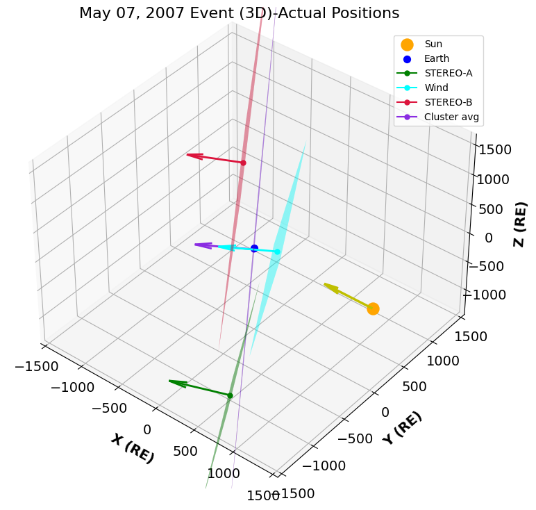
(a)

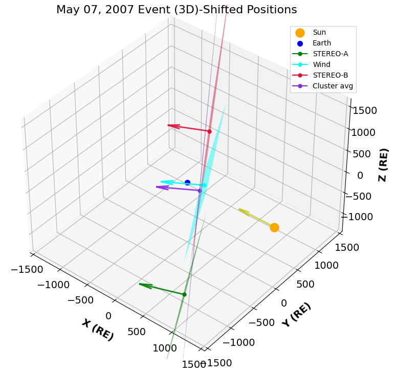
(b)

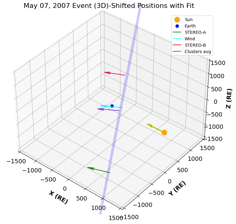
(c)

Figure 5.22: A 3D sketch of the propagation of the IP shock through spacecraft– Wind, STEREO$-$A, and STEREO$-$B, and average position of 4 Cluster satellites. (a) Actual shock detected positions. (b) The positions of STEREO$-$A, STEREO$-$B, and the average positions of 4 Clusters are shifted back in time to the shock detection time of the Wind spacecraft. (c) The time-shifted positions are fitted with a plane. The arrows indicate the normal vector direction and the planes perpendicular to the normal vectors indicate the shock surface orientations. The sizes of the planes are arbitrary.

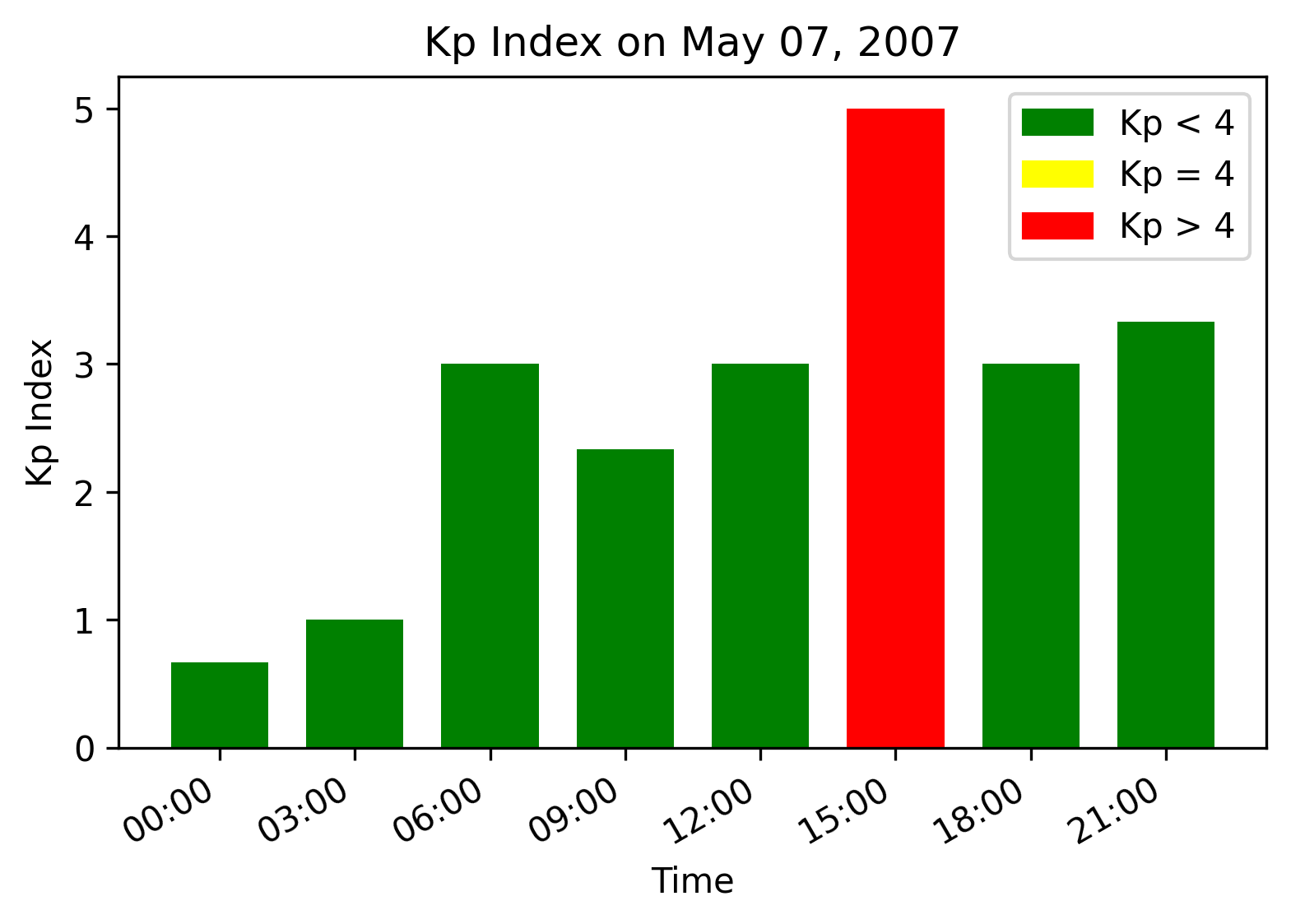
Figure 5.23: Kp-index on May 07, 2007. The green bar indicates moderate geomagnetic activity, while the yellow bar denotes intensifying geomagnetic activity with the red bar being a geomagnetic storm. Here, the red bar indicates a G1-minor geomagnetic storm.

5.2.4 The Event April 23, 2007

Here I list all magnetic field observations of the spacecraft for the event and apply the minimum variance analysis (MVA) and the magnetic coplanarity (CP) methods to them. In this event, the order between upstream and downstream is swapped because it is a fast-reverse (FR) shock event, which means the shock is up against its driver. The upstream and downstream time intervals that most agree between the minimum variance analysis (MVA) and the magnetic coplanarity methods (CP) for all the spacecraft are shown in Table 5.6 and their corresponding Figures are 5.24 for the STEREO$-$A, 5.25 for the ACE, 5.26 for the Wind, and 5.27 for the STEREO$-$B. Table 5.6 also shows the ratio between the intermediate eigenvalue $\lambda_{2}$ and the smallest eigenvalue $\lambda_{3}$ as well as the angle between the MVA normal and CP normals in the determined upstream and downstream time intervals for each spacecraft.

Implementation of the methods on the event April 23, 2007

Spacecraft	$\Delta t_{down}$	$\Delta t_{up}$	$\lambda_{2}/\lambda_{3}$	$\Delta\theta_{MVA-CP}$
STEREO$-$A	(06:46:00 - 06:52:23)	(06:57:03 - 07:02:34)	3.29	$1.07^{\circ}$
ACE	(08:51:30 - 08:56:30)	(09:03:00 - 09:07:00)	4.22	$3.435^{\circ}$
Wind	(09:04:00 - 09:10:00)	(09:12:20 - 09:13:15)	3.38	$1.46^{\circ}$
STEREO$-$B	(13:15:45 - 13:20:00)	(13:24:00 - 13:26:00)	8.18	$1.67^{\circ}$

Table 5.6: Here, $\Delta t_{down}$ denotes the defined downstream and $\Delta t_{up}$ denotes the defined upstream time intervals with MVA and CP analysis methods. $\lambda_{3}/\lambda_{2}$ indicates the ratio between the intermediate eigenvalue $\lambda_{2}$ and the smallest eigenvalue $\lambda_{2}$, and $\Delta\theta_{MVA-CP}$ is the angle between the MVA and CP normals.

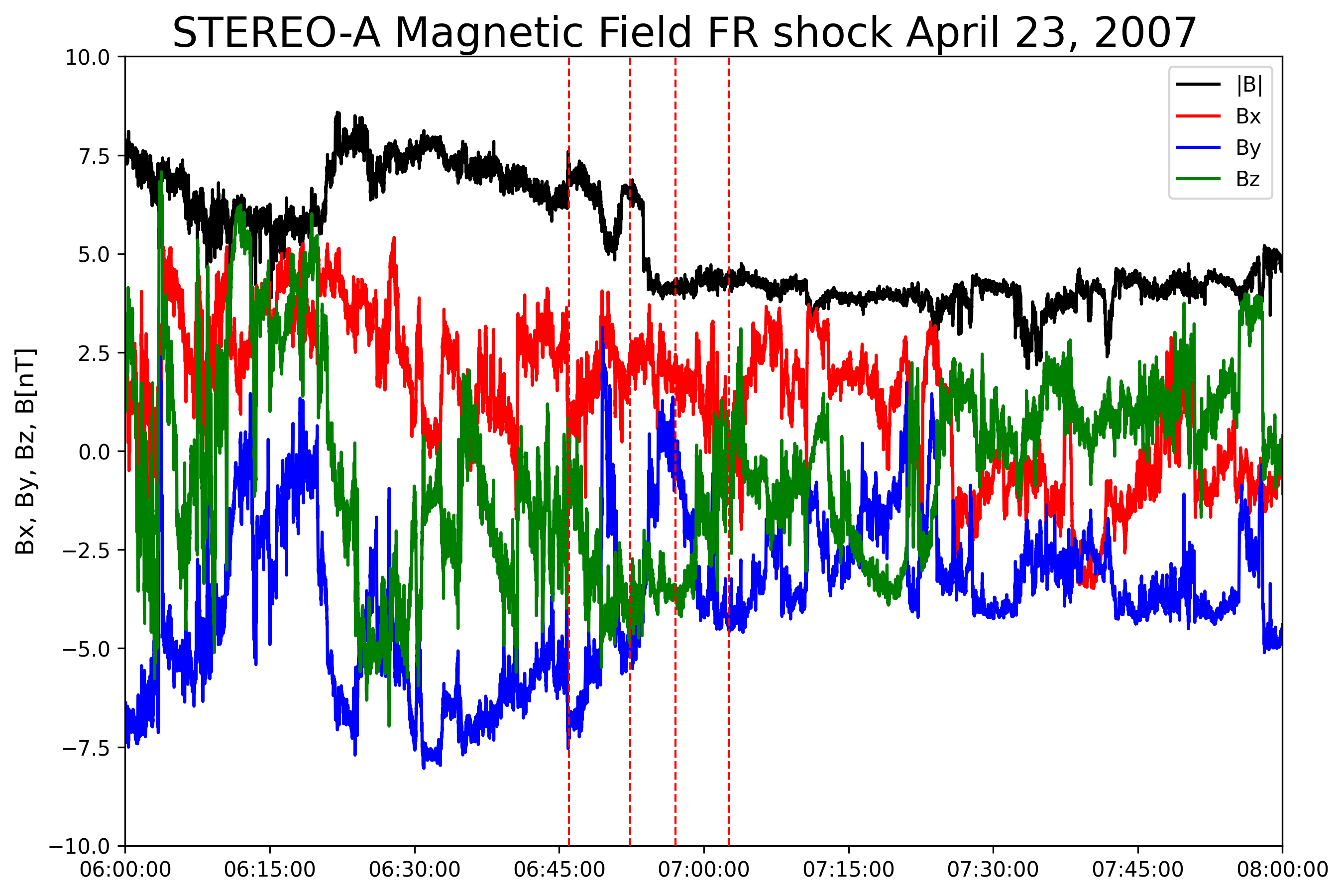
Figure 5.24: The STEREO$-$A magnetic field measurements. The downstream $\Delta t_{down}$ is between (06:46:00 - 06:52:23), and the upstream $\Delta t_{up}$ is between (06:57:03 - 07:02:34). FR stands for the fast reverse shock, which means the shock is moving toward its driver. The chosen intervals of the upstream and downstream magnetic field. The red dashed lines each represent the downstream starting time and ending time and the upstream starting time and ending time respectively

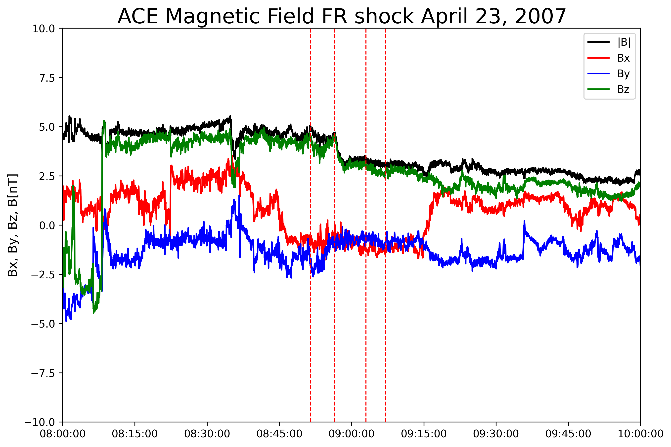
Figure 5.25: ACE magnetic field measurements. The downstream $\Delta t_{down}$ is between (08:51:30 - 08:56:30), and the upstream $\Delta t_{up}$ is between (09:03:00 - 09:07:00). The symbols and details of the figures are the same as 5.24

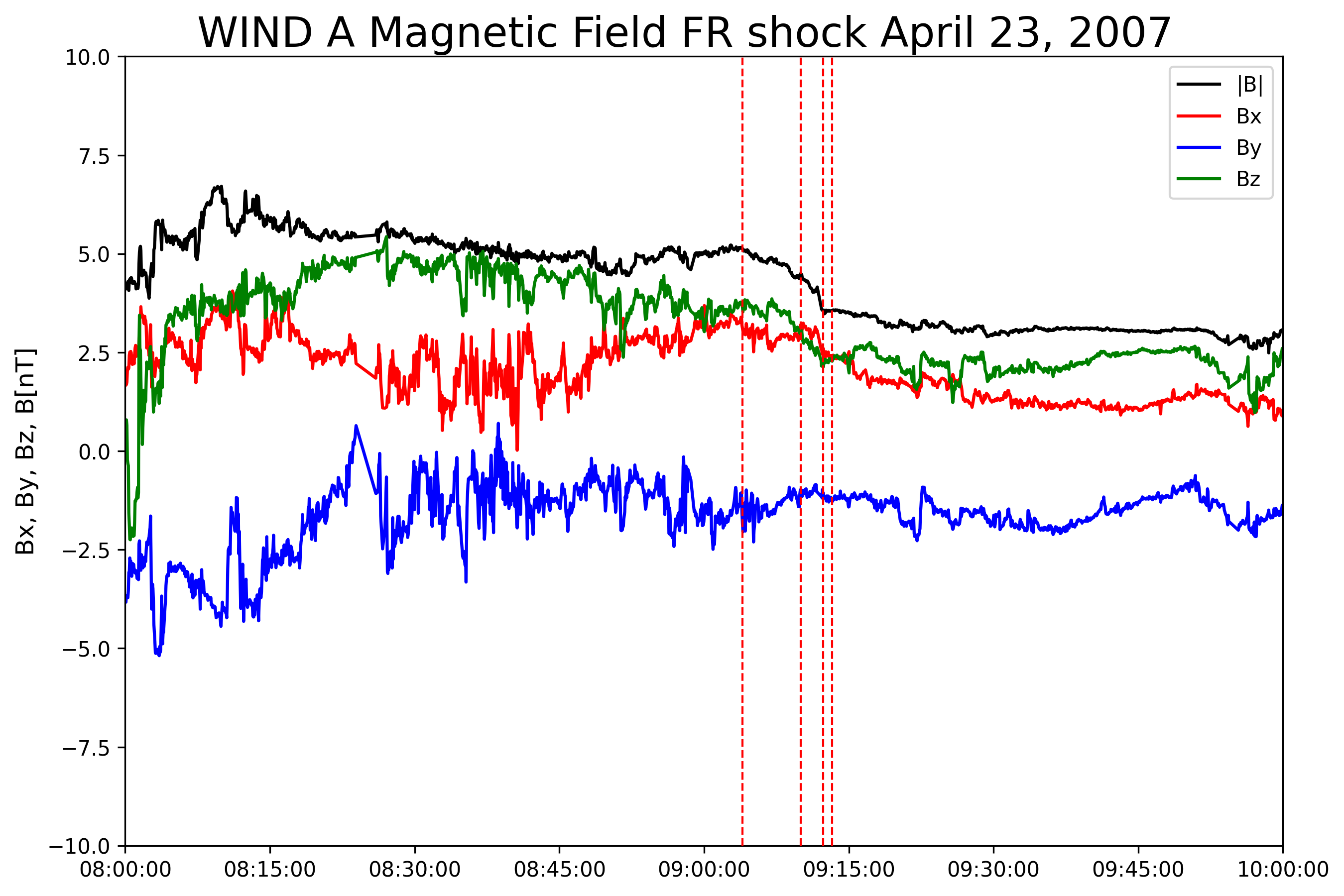
Figure 5.26: The Wind magnetic field measurements. The downstream $\Delta t_{down}$ is between (09:04:00 - 09:10:00), and the upstream $\Delta t_{up}$ is between (09:12:20 - 09:13:15). The symbols and details of the figures are the same as 5.24

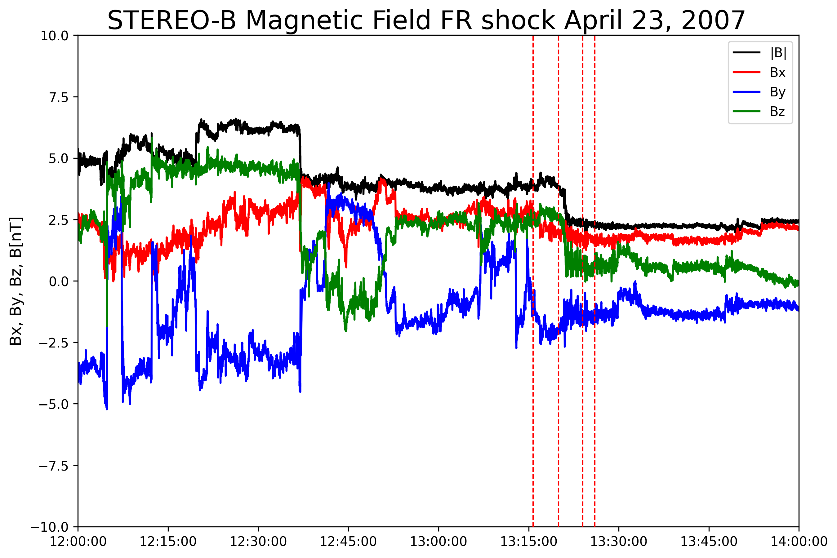
Figure 5.27: STEREO$-$B magnetic field measurements. The downstream $\Delta t_{down}$ is between (13:15:45 - 13:20:00), and the upstream $\Delta t_{up}$ is between (13:24:00 - 13:26:00). The symbols and details of the figures are the same as 5.24

5.2.5 Analysis of the Event April 23, 2007

Similarly to the event about, the upstream and downstream time intervals are highly accurate as well, considering the angle difference between the two methods is minimal and the eigenvalue criteria are fulfilled for each spacecraft data.

Also, using the determined time intervals, the estimations of the ratio between the upstream and downstream magnetic field, densities, and temperatures as well as the bulk speed, and shock $\theta_{Bn}$ angle are made. These parameters, the minimum variance analysis normal and the magnetic coplanarity normal are shown in Table 5.7, where also the solar wind bulk speed and the downstream to upstream ratios for the shock criteria are fulfilled accordingly with 4.14 and 4.15, and the STEREO$-$B ratios are compatible with the shock criteria, proving that the STEREO$-$B did detect the shock. However, the shock detected by the STEREO$-$B appears to become quasi-parallel a few hours after the shock detection times of STEREO$-$A, ACE, and the Wind based on the shock $\theta_{Bn}$ angle, see Table 5.9, where the calculated results of additional parameters are shown.

Spacecraft $B_{d}/B_{u}$ $N_{d}/N_{u}$ $T_{d}/T_{u}$ $\Delta V$ $\theta_{Bn}$ Spacecraft MVA Coplanarity $\Delta\theta_{MVA-CP}$ STEREO$-$A $1.470\pm 0.16$ $2.000\pm 0.70$ $1.480\pm 0.50$ $46.00\pm 13$ 88.40 STEREO$-$A [-0.86, 0.020, -0.502] [-0.858, 0.007, -0.51] 1.070 ACE $1.410\pm 0.08$ $1.440\pm 0.16$ $1.220\pm 0.09$ $23.720\pm 5.57$ 46.2 ACE [0.872, -0.189, -0.450] [0.869, -0.232, -0.434] 2.653 Wind $1.349\pm 0.06$ $1.424\pm 0.40$ $1.285\pm 0.7$ $19.26\pm 0.13$ 61.85 Wind [-0.823, 0.430, 0.369] [-0.809, 0.438, 0.390] 1.349 STEREO$-$B $1.730\pm 0.09$ $1.980\pm 0.14$ $1.340\pm 0.15$ $21.20\pm 3.4$ 29.39 STEREO$-$B [-0.751, 0.591, 0.292] [-0.731, 0.610, -0.303] 1.67

Table 5.7: Resulting core parameters of studying the data of the STEREO$-$A, STEREO$-$B, ACE, and Wind spacecraft. Here $\theta_{Bn}$ is the shock $\theta$ angle.

Table 5.8: (Continued) Resulting core parameters of studying the data of the STEREO$-$A, STEREO$-$B, ACE, and Wind spacecrafts. $\theta_{MVA-CP}$ is the angle difference between the minimum variance normal vectors and the magnetic coplanarity normal vectors.

Spacecraft $V_{sh}$ km/s $C^{up}_{s}$ km/s $V^{up}_{A}$ km/s $C^{up}_{ms}$ km/s Spacecraft Plasma $\beta_{up}$ Alfvén Mach Magnetosonic Mach STEREO$-$A 467.95 $64.97\pm 7.74$ $68.715\pm 29.2$ $94.57\pm 21.85$ STEREO$-$A $1.07\pm 0.94$ $0.998\pm 0.67$ $0.725\pm 0.41$ ACE 412.36 $58.28\pm 4.94$ $52.82\pm 15.90$ $78.66\pm 11.26$ ACE $1.46\pm 0.91$ $1.49\pm 0.56$ $1.0\pm 0.27$ Wind 372.59 $56.14\pm 5.36$ $56.22\pm 14.71$ $79.45\pm 11.08$ Wind $1.19\pm 0.66$ $1.24\pm 0.52$ $0.88\pm 0.31$ STEREO$-$B 370.31 $57.31\pm 5.38$ $29.045\pm 12.28$ $64.25\pm 07.34$ STEREO$-$B $4.67\pm 4.04$ $1.688\pm 1.08$ $0.763\pm 0.37$

Table 5.9: Resulting additional parameters of studying the data of the three spacecraft. $V_{sh}$ is the shock speed, $C^{up}_{s}$ is the upstream sound speed, $V^{up}_{A}$ is the upstream Alfvén speed and $C^{up}_{ms}$ is the upstream magnetosonic speed.

Table 5.10: (Continued) Resulting additional parameters of studying the data of the three spacecraft. Plasma $\beta_{up}$, Alfvén Mach, and Magnetosonic Mach are shown

Similarly, the sketches of the IP shocks that were detected by the spacecraft are shown in 5.28(a), 5.28(b), 5.28(c). In these 2D sketches, the shock propagation and normal vector orientation are shown in a temporal development manner.

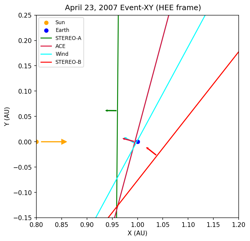
(a)

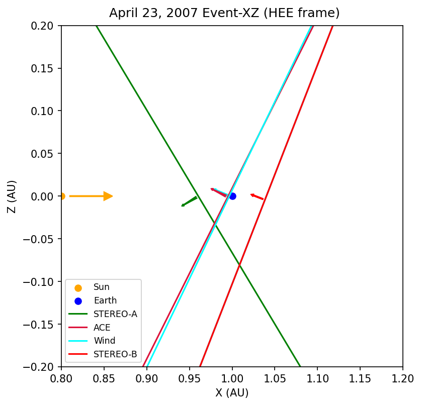
(b)

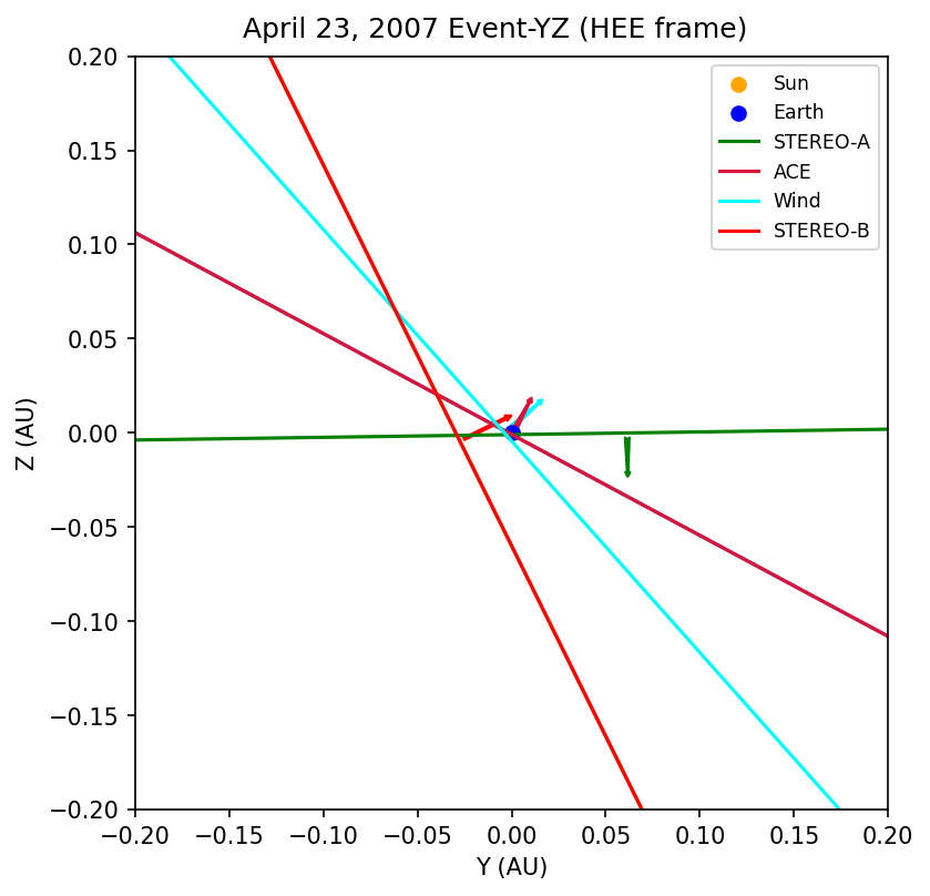
(c)

Figure 5.28: 2D XY, XZ, and YZ sketches of the propagation of the IP shock through spacecraft– STEREO$-$A, ACE, Wind, and STEREO$-$B. The orange arrow represents the Sun-Earth line direction. The arrows on spacecraft positions indicate the normal vector direction and the lines perpendicular to the normal vectors indicate the shock surface orientations. The sizes of the lines are arbitrary.

5.2.6 Discussion of the Event April 23, 2007

The 3D sketch is shown in 5.30, and in the 3D sketch, the Wind, ACE, and STEREO$-$B positions are time-shifted to the STEREO$-$A’s position to see the overall shape of this IP shock. It appears the shape of the shock is not uniform and is twisted from the STEREO$-$A spacecraft to the other three spacecraft in the Z-axis along the transverse direction (Y-axis) to the Sun-Earth line, see Figure 5.28(b). As seen from Figure 5.30(c), the STEREO$-$A alone is on the dusk (left) side of the Sun-Earth line while the Wind, the ACE, and the STEREO$-$B are on the dawn (right). In this XY-plane view, the shock normal vectors appear to be changing or slightly rotating their direction from the STEREO$-$A to the Wind, the ACE, and the STEREO$-$B along Y-axis, and the shock is changing from the quasi-perpendicular to quasi-parallel based on the shock $\theta_{Bn}$ angle. This IP shock is a fast reverse shock, meaning it travels toward the Sun even though the shock propagates away from the Sun with the solar wind. The shock detection time between the STEREO$-$A and the Wind/ACE is about two hours while the between STEREO$-$A and B is almost six hours, yet the shock orientation is significantly changed from the STEREO$-$A to the other three spacecraft indicating the change is spatial, not temporal. So, due to this nature, the IP shock could be a local ripple. The ripples on the shock surface are known for being caused by ICME (interplanetary coronal mass ejections) shock drivers as they do not propagate into homogeneous interplanetary medium (Acuña et al., 2008). However, the source of this event is a stream-interaction region (SIR) as listed here https://stereo-ssc.nascom.nasa.gov/pub/ins_data/impact/level3/STEREO_Level3_Shock.pdf. I determined the Kp-index of this event as seen in Figure 5.29. Similar to the fast-forward shock event of May 07, 2007, a G1-minor geomagnetic storm occurred on this day, but the beginning of the geomagnetic storm happened three hours before the shock detection time of the STEREO$-$A while the ending of the storm was partially at the same time as the STEREO$-$A. As stated before, SIR/CIRs form when the fast-moving solar wind catches the slow-moving solar wind (Richardson, 2018). This sometimes forms a pair of shocks, one leading as a fast-forward shock while a rarefied shock trails the solar wind as a fast-reverse shock but oftentimes as just sole fast-forward or fast reverse shocks (Jian et al., 2019). Nevertheless, since it always involves the fast-moving solar wind, it makes total sense why the G1-minor geomagnetic storm with a Kp-5 index happened before the detection of the shock because it seems the fast-moving solar wind caused the minor storm before the fast-reverse shock finally arrived at the spacecraft positions. The normal orientation inconsistency can also be explained by the argument that this shock is a fast-reverse shock because SIRs have characteristic tilts such that forward waves direct towards the solar equatorial plane while the reverse waves tend to move in the direction of the solar poles (Kilpua et al., 2015). Hence, this tilting nature may explain the XZ component tilted orientation between the STEREO$-$A and the other three spacecraft – the Wind, the ACE, and the STEREO$-$B.

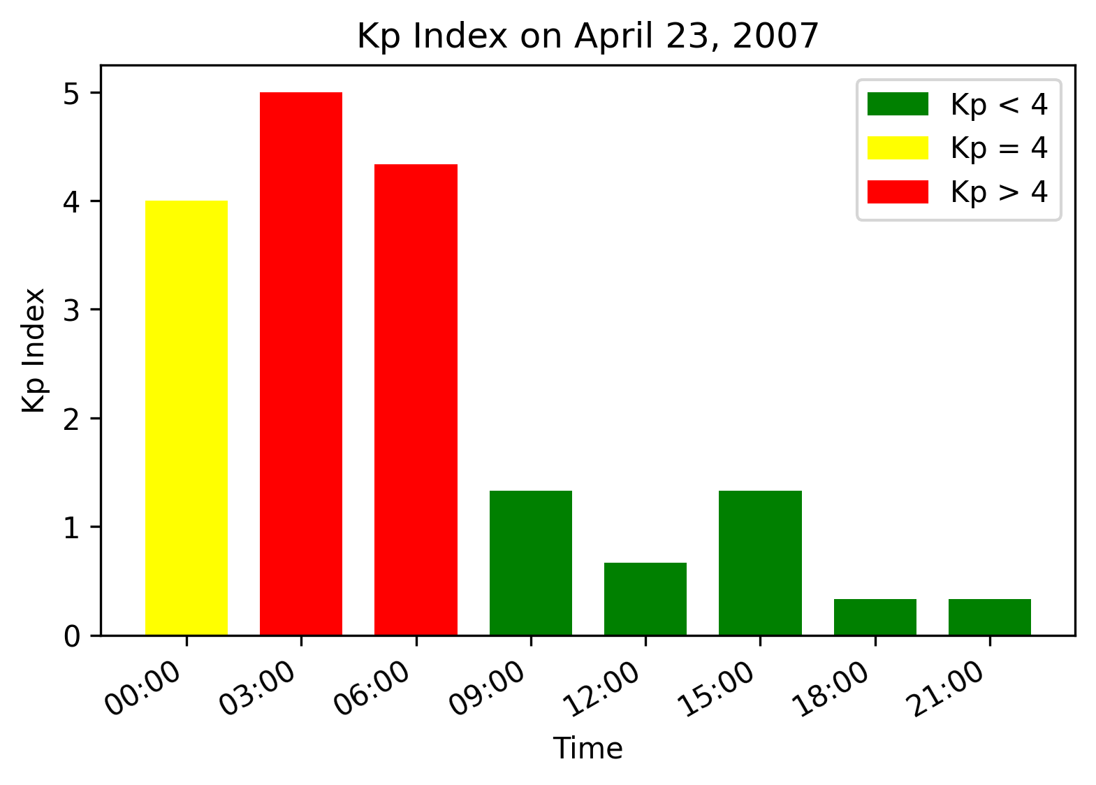
Figure 5.29: The Kp-index on April 23, 2007. The symbols and details of the Figure is the same as 5.23

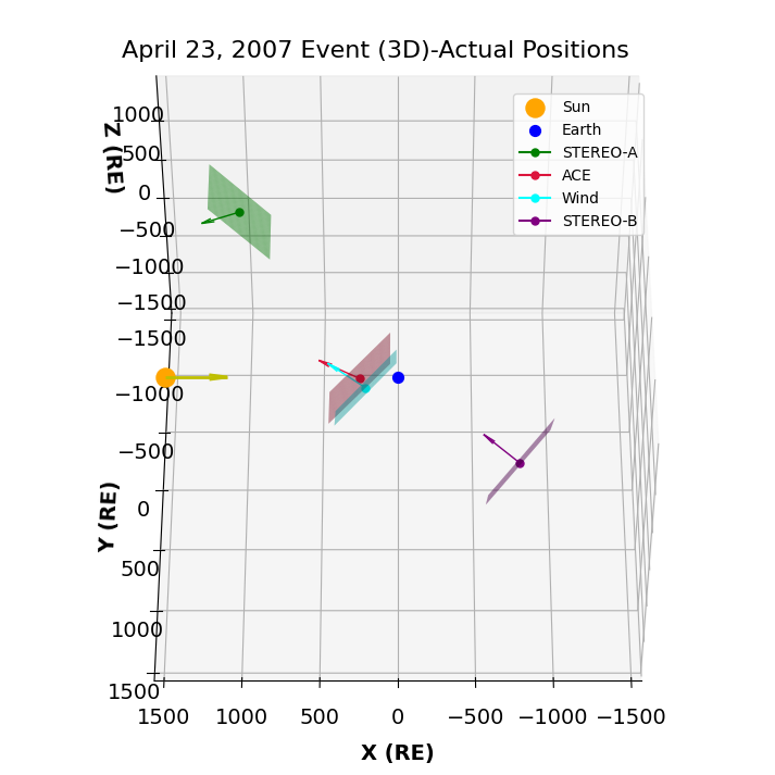
(a)

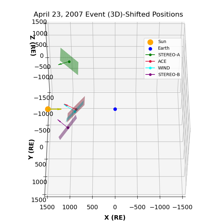
(b)

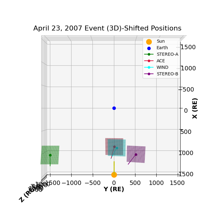
(c)

Figure 5.30: (a) A 3D sketch of the propagation of the IP shock through 3 spacecraft– STEREO$-$A, Wind, ACE, and STEREO$-$B. (b) The positions of Wind, ACE, and STEREO$-$B are shifted back in time to the shock detection time of STEREO$-$A. (C) The shifted positions are shown from the top view. The arrows indicate the normal vector direction and the planes perpendicular to the normal vectors indicate the shock surface orientations. The sizes of the planes are arbitrary.

Chapter 6 Summary and conclusions

In this thesis, a single spacecraft study of the interplanetary (IP) shock is presented. This thesis aims to study and determine how IP shocks are developing and evolving in spatial and temporal propagation. For this purpose, two methods are implemented, namely the minimum variance analysis of the magnetic field (MVA) and the magnetic coplanarity methods (CP) for the determination of upstream and downstream time intervals. The two methods use magnetic field measurement data, which is known for its high resolutions compared to those of plasma data concerning their respective heliospheric variational rates. To acquire data, I used the Coordinated Data Analysis Web (CDAWeb) of NASA for each spacecraft. Data are in the first event case – from early morning to noon in 2007-05-07 for seven different spacecraft, namely Wind, Stereo A and B, and 4 Cluster satellites.

The second event case, similarly, - from early morning to noon in 2007-04-23 for four different spacecraft, namely Wind, STEREO$-$A and B, and ACE. After acquiring data, I changed every coordinate system of the data to the HEE coordinate system so that it is easy to compare the data and how the shock parameters change when propagating through space. However, near Earth, vectors are changed to the GSE coordinate system. For accepting the upstream and downstream time intervals, two criteria are made such as the $\theta$ angle differences between MVA and the magnetic coplanarity must be considerably small, $<15^{\circ}$, and the ratio between the intermediate eigenvalue to the smallest eigenvalue must be greater than 3. For both case studies, I found such upstream and downstream intervals, indicating the results are highly accurate. Hence, pinpointing the shock formations has been very successful due to using the two methods to determine the shock normal vectors.

The two event studies are not timely ordered. First, the Event May 07, 2007, is studied, and then the Event April 23, 2007, is followed. Hence the Event May 07 is referred to as the first event and the Event April 23 is the second event. The first event is a fast-forward (FF) shock event, the shock propagating away from the Sun in the solar wind frame of reference in addition to the solar wind on which it propagates is also traveling away from the Sun. The shock parameters agree within the errors. From the 2D sketches as well as the 3D sketch, on which the positions of the STEREO$-$A and B, and 4 Clusters spacecraft are time-shifted to the shock detection time of the Wind spacecraft to see the geometry of the shock, the shock appears planar and tilted $56.42^{\circ}$ to the Sun-Earth line, explaining why the Wind first detected the IP shock even though its location is behind the STEREO$-$A in respect to the Sun-Earth line. The tilt of this planar shock surface is almost identical to the usual propagation of the Parker spiral impacting the Earth. Consequently, this indicates the origin of the shock is co-rotating stream interactions (CIRs), which agrees with the detected CIR on that day. There is no sign of temporal change in this scale. In the spatial range of 40 million km, no change was observable. The G1-minor geomagnetic storm happened after this shock was detected, indicating this shock event caused the geomagnetic storm on that day.

The second event is the fast reverse (FR) shock event, the shock propagates toward the Sun in the solar wind frame of reference although the shock propagates away from the Sun with its carrier solar wind. There are several peculiarities with this shock event, it appears the shape of the shock is not uniform and twisted from the STEREO$-$A spacecraft to the other spacecraft along the transverse direction to the Sun-Earth line. The shock normal vectors also were observed to be changing along Y-axis. A G1-minor geomagnetic storm occurred on this day, similar to the fast-forward shock event of May 07, 2007. Intriguingly, the onset of this storm took place three hours prior to the shock detection time recorded by STEREO$-$A. The termination of the storm partially coincided with the STEREO$-$A detection time. The formation of Stream Interaction Regions/Corotating Interaction Regions (SIR/CIRs) occurs when a faster solar wind stream encounters a slower one. The source of this shock is SIR/CIR. Given the involvement of fast-moving solar wind, it’s logical that the G1-minor geomagnetic storm, with a Kp-5 index, began before the shock detection. It appears that the fast-moving solar wind instigated the minor storm prior to the arrival of the fast-reverse shock at the spacecraft’s position. The orientation irregularity can be potentially accounted for by the characteristic tilts of SIRs. The forward waves of SIRs tend to propagate towards the solar equatorial plane, while the reverse waves lean towards the solar poles. This inherent tilting could explain the tilted orientation of the XZ component observed between the STEREO$-$A and the other three spacecraft – Wind, ACE, and STEREO$-$B. Even without this characteristic tilting, the fast-reverse shock is being compressed, which, given its defining nature, could explain the irregularities.

References

- Acuña et al. [2008] MH Acuña, D Curtis, JL Scheifele, CT Russell, P Schroeder, A Szabo, and JG Luhmann. The stereo/impact magnetic field experiment. Space Science Reviews, 136:203–226, 2008.
- Alfvén [1942] Hannes Alfvén. Existence of electromagnetic-hydrodynamic waves. Nature, 150(3805):405–406, 1942.
- Antonsen Jr. [2019] T. M. Antonsen Jr. Single fluid ideal mhd phys 761 physics 761, October 2019. https://terpconnect.umd.edu/~antonsen/PHYS761_F19/LECTURES/Single_Fluid_MHD.pdf.
- Aschwanden [2006] Markus Aschwanden. Physics of the solar corona: an introduction with problems and solutions. Springer Science & Business Media, 2006.
- Aschwanden [2014] MJ Aschwanden. Encyclopedia of the solar system, 2014.
- Babcock and Babcock [1955] Horace W Babcock and Harold D Babcock. The sun’s magnetic field, 1952-1954. The Astrophysical Journal, 121:349, 1955.
- Balogh et al. [1997] A Balogh, MW Dunlop, SWH Cowley, DJ Southwood, JG Thomlinson, KH Glassmeier, G Musmann, H Lühr, S Buchert, MH Acuna, et al. The cluster magnetic field investigation. Space Science Reviews, 79:65–91, 1997.
- Bartels [1949] J Bartels. The standardized index ks, and the planetary index kp, iatme bull., 12 (b), 97; iugg publ. Office, Paris, 1949.
- Basu and Antia [2007] Sarbani Basu and H. M. Antia. Helioseismology and solar abundances. Physics Reports, 457:217–283, 2007.
- Basu et al. [2009] Sarbani Basu, William J Chaplin, Yvonne Elsworth, Roger New, and Aldo M Serenelli. Fresh insights on the structure of the solar core. The Astrophysical Journal, 699(2):1403, 2009.
- Baumjohann and Nakamura [2007] W. Baumjohann and R. Nakamura. 5.03 - magnetospheric contributions to the terrestrial magnetic field. In Gerald Schubert, editor, Treatise on Geophysics, pages 77–92. Elsevier, Amsterdam, 2007. ISBN 978-0-444-52748-6. doi: https://doi.org/10.1016/B978-044452748-6.00088-2. URL https://www.sciencedirect.com/science/article/pii/B9780444527486000882.
- Baumjohann and Treumann [2012] Wolfgang Baumjohann and Rudolf A Treumann. Basic space plasma physics (revised edition). World Scientific Publishing Company, 2012.
- Berdichevsky et al. [2000] Daniel B Berdichevsky, Adam Szabo, Ronald P Lepping, Adolfo F Viñas, and Franco Mariani. Interplanetary fast shocks and associated drivers observed through the 23rd solar minimum by wind over its first 2.5 years. Journal of Geophysical Research: Space Physics, 105(A12):27289–27314, 2000.
- Biermann [2013] Ludwig F Biermann. 25. solar corpuscular radiation and the interplanetary gas. In A Source Book in Astronomy and Astrophysics, 1900–1975, pages 147–148. Harvard University Press, 2013.
- Bittencourt [2004] José A Bittencourt. Fundamentals of plasma physics. Springer Science & Business Media, 2004.
- Bougeret et al. [1995] J L Bougeret, M L Kaiser, Paul J Kellogg, Robert Manning, K Goetz, SJ Monson, N Monge, L Friel, CA Meetre, C Perche, et al. Waves: The radio and plasma wave investigation on the wind spacecraft. Space Science Reviews, 71:231–263, 1995.
- Bougeret et al. [2008] Jean-Louis Bougeret, K Goetz, ML Kaiser, SD Bale, PJ Kellogg, M Maksimovic, N Monge, SJ Monson, PL Astier, S Davy, et al. S/waves: The radio and plasma wave investigation on the stereo mission. Space Science Reviews, 136:487–528, 2008.
- Brummell et al. [1995] Nicholas Brummell, Juri Toomre, and Fausto Cattaneo. Turbulent dynamics in the solar convection zone. Science, 269(5229):1370–1379, 1995.
- Burlaga [2015] L Burlaga. Voyager observations of the magnetic field in the heliosheath and the local interstellar medium. In Journal of Physics: Conference Series, volume 642, page 012003. IOP Publishing, 2015.
- Cane and Lario [2006] HV Cane and D Lario. An introduction to cmes and energetic particles. Space science reviews, 123(1):45–56, 2006.
- Center/SDO [2015] NASA’s Goddard Space Flight Center/SDO. Sdo solar comparison october 2010 to october 2012, 2015.
- Chakraborty and Basak [2022] Sayak Chakraborty and Tamal Basak. Brief review on lower ionosphere and the effects of solar flare thereon. Advances in Modern and Applied Sciences, page 137, 2022.
- Chao and Hsieh [1984] J.K. Chao and K.C. Hsieh. On determining magnetohydrodynamic shock parameters bn and ma. Planetary and Space Science, 32(5):641–646, 1984. ISSN 0032-0633. doi: https://doi.org/10.1016/0032-0633(84)90115-6. URL https://www.sciencedirect.com/science/article/pii/0032063384901156.
- Chemin [2022] Yann-Henri Chemin. Introductory chapter: The sun and its phenomenal material flux. In Magnetosphere and Solar Winds, Humans and Communication. IntechOpen, 2022.
- Christensen-Dalsgaard et al. [1991] J Christensen-Dalsgaard, DO Gough, and MJ Thompson. The depth of the solar convection zone. The Astrophysical Journal, 378:413–437, 1991.
- Cid et al. [2014] Consuelo Cid, Judith Palacios, Elena Saiz, Antonio Guerrero, and Yolanda Cerrato. On extreme geomagnetic storms. Journal of Space Weather and Space Climate, 4:A28, 2014.
- CIS team [2021] CIS team. Cluster active archive: Cis user guide. https://caa.esac.esa.int/documents/UG/CAA_EST_UG_CIS_v37.pdf, 2021.
- Cornilleau-Wehrlin et al. [1997] Nicole Cornilleau-Wehrlin, P Chauveau, S Louis, A Meyer, JM Nappa, S Perraut, L Rezeau, P Robert, A Roux, C De Villedary, et al. The cluster spatio-temporal analysis of field fluctuations (staff) experiment. The Cluster and Phoenix Missions, pages 107–136, 1997.
- Cowen [2013] Ron Cowen. Voyager 1 has reached interstellar space, 2013.
- Cranmer [2009] Steven R Cranmer. Coronal holes. Living Reviews in Solar Physics, 6(1):1–66, 2009.
- Daly and Kronberg [2010] Patrick W Daly and Elena A Kronberg. Rapid products at the cluster active archive. In The Cluster Active Archive: Studying the Earth’s Space Plasma Environment, pages 145–158. Springer, 2010.
- David Burgess [2017] David Burgess. Theory of particle acceleration at collisionless shocks les houches 2017, 2017. https://ipag.osug.fr/~lesurg/plasmas2017/talks/Burgess-Houches-2017.pdf/, Last accessed on 2022-04-04.
- Davidson [2002] Peter Alan Davidson. An introduction to magnetohydrodynamics, 2002.
- Décréau et al. [1997] PME Décréau, P Fergeau, V Krannosels’ Kikh, M Lévêque, Ph Martin, O Randriamboarison, FX Sené, JG Trotignon, P Canu, and PB Mögensen. Whisper, a resonance sounder and wave analyser: Performances and perspectives for the cluster mission. Space Science Reviews, 79(1-2):157–193, 1997.
- Dr. David H. Hathaway [2015] dave.hathaway Dr. David H. Hathaway. The solar interior, 2015.
- Escoubet et al. [1997] CP Escoubet, R Schmidt, and ML Goldstein. Cluster–science and mission overview. Space Science Reviews, 79(1-2):11–32, 1997.
- Escoubet et al. [2001] CP Escoubet, M Fehringer, and M Goldstein. The cluster mission-introduction. In Annales Geophysicae, volume 19, pages 1197–1200. EUROPEAN GEOPHYSICAL SOC MAX-PLANCK-STR 13, 37191 KATLENBURG-LINDAU, GERMANY, 2001.
- Facskó et al. [2008] Gabor Facskó, Karoly Kecskeméty, G Erdős, Mariella Tátrallyay, Patrick W Daly, and Iannis Dandouras. A statistical study of hot flow anomalies using cluster data. Advances in space research, 41(8):1286–1291, 2008.
- Facskó et al. [2009] Gabor Facskó, Zoltan Nemeth, G Erdős, Arpad Kis, and Iannis Dandouras. A global study of hot flow anomalies using cluster multi-spacecraft measurements. In Annales geophysicae, volume 27, pages 2057–2076. Copernicus Publications Göttingen, Germany, 2009.
- Facskó et al. [2010] Gábor Facskó, Jean-Gabriel Trotignon, Iannis Dandouras, Elisabeth A Lucek, and Patrick W Daly. Study of hot flow anomalies using cluster multi-spacecraft measurements. Advances in space research, 45(4):541–552, 2010.
- Facskó et al. [2022] Gábor Facskó, Biró Nikolett, Kobán Gergely, and Munkjargal Lkhagvadorj. Space weather effects on critical infrastructure. In Nyikes Zoltán and Anna Kovács Tünde, editors, ICCECIP 2022 4th International Conference on Central European Critical Infrastructure Protection: Abstract Book, pages 25–25, Bp, Hungary, 2022. Obuda University.
- Feldman et al. [2005] U Feldman, E Landi, and NA Schwadron. On the sources of fast and slow solar wind. Journal of Geophysical Research: Space Physics, 110(A7), 2005.
- Fitzpatrick [2014] Richard Fitzpatrick. Plasma physics: an introduction. Crc Press, 2014.
- Freidberg [2014] Jeffrey P Freidberg. ideal MHD. Cambridge University Press, 2014.
- Galvin et al. [2008] Antoinette B Galvin, Lynn M Kistler, Mark A Popecki, Charlie J Farrugia, Kristin DC Simunac, Lorna Ellis, E Möbius, Martin A Lee, M Boehm, J Carroll, et al. The plasma and suprathermal ion composition (plastic) investigation on the stereo observatories. Space Science Reviews, 136(1):437–486, 2008.
- García et al. [2007] Rafael A García, Sylvaine Turck-Chièze, Sebastian J Jiménez-Reyes, Jérôme Ballot, Pere L Pallé, Antonio Eff-Darwich, Savita Mathur, and Janine Provost. Tracking solar gravity modes: the dynamics of the solar core. Science, 316(5831):1591–1593, 2007.
- Genot et al. [2018] V Genot, B Renard, N Dufourg, M Bouchemit, N Lormant, L Beigbeder, D Popescu, J-P Toniutti, N André, F Pitout, et al. Treps, a tool for coordinate and time transformations in space physics. Planetary and Space Science, 150:86–90, 2018.
- Gilbert [2003] Andrew D. Gilbert. Chapter 9 - dynamo theory. volume 2 of Handbook of Mathematical Fluid Dynamics, pages 355–441. North-Holland, 2003. doi: https://doi.org/10.1016/S1874-5792(03)80011-3. URL https://www.sciencedirect.com/science/article/pii/S1874579203800113.
- Gloeckler et al. [1995] G Gloeckler, H Balsiger, A Bürgi, P Bochsler, LA Fisk, AB Galvin, J Geiss, F Gliem, DC Hamilton, TE Holzer, et al. The solar wind and suprathermal ion composition investigation on the wind spacecraft. Space Science Reviews, 71:79–124, 1995.
- Gloeckler et al. [1998] G Gloeckler, J Cain, FM Ipavich, EO Tums, P Bedini, LA Fisk, TH Zurbuchen, P Bochsler, J Fischer, RF Wimmer-Schweingruber, et al. Investigation of the composition of solar and interstellar matter using solar wind and pickup ion measurements with swics and swims on the ace spacecraft. The advanced composition explorer mission, pages 497–539, 1998.
- Goedbloed et al. [2019] Hans Goedbloed, Rony Keppens, and Stefaan Poedts. Magnetohydrodynamics: Of Laboratory and Astrophysical Plasmas. Cambridge University Press, 2019.
- Gonzalez et al. [1994] WD Gonzalez, Jo-Ann Joselyn, Yohsuke Kamide, Herb W Kroehl, G Rostoker, BT Tsurutani, and VM Vasyliunas. What is a geomagnetic storm? Journal of Geophysical Research: Space Physics, 99(A4):5771–5792, 1994.
- Gurnett et al. [1997] DA Gurnett, RL Huff, and DL Kirchner. The wide-band plasma wave investigation. The Cluster and Phoenix Missions, pages 195–208, 1997.
- Gustafsson et al. [1997] G Gustafsson, R Boström, B Holback, G Holmgren, A Lundgren, K Stasiewicz, L Åhlén, FS Mozer, D Pankow, P Harvey, et al. The electric field and wave experiment for the cluster mission. The Cluster and Phoenix Missions, pages 137–156, 1997.
- Haaland et al. [2007] SE Haaland, G Paschmann, Matthias Förster, JM Quinn, RB Torbert, CE McIlwain, H Vaith, PA Puhl-Quinn, and CA Kletzing. High-latitude plasma convection from cluster edi measurements: method and imf-dependence. In Annales Geophysicae, volume 25, pages 239–253. Copernicus Publications Göttingen, Germany, 2007.
- Harten and Clark [1995] Ronald Harten and Kenn Clark. The design features of the ggs wind and polar spacecraft. Space Science Reviews, 71(1):23–40, 1995.
- Heber et al. [1999] B Heber, TR Sanderson, and M Zhang. Corotating interaction regions. Advances in Space Research, 23(3):567–579, 1999.
- Howard et al. [2008] Russell A Howard, JD Moses, Angelos Vourlidas, JS Newmark, Dennis G Socker, Simon P Plunkett, Clarence M Korendyke, JW Cook, A Hurley, JM Davila, et al. Sun earth connection coronal and heliospheric investigation (secchi). The STEREO Mission, pages 67–115, 2008.
- Jian et al. [2019] LK Jian, JG Luhmann, CT Russell, and AB Galvin. Solar terrestrial relations observatory (stereo) observations of stream interaction regions in 2007–2016: Relationship with heliospheric current sheets, solar cycle variations, and dual observations. Solar physics, 294(3):31, 2019.
- Johlander et al. [2022] Andreas Johlander, Markus Battarbee, Lucile Turc, Urs Ganse, Yann Pfau-Kempf, Maxime Grandin, Jonas Suni, Vertti Tarvus, Maarja Bussov, Hongyang Zhou, et al. Quasi-parallel shock reformation seen by magnetospheric multiscale and ion-kinetic simulations. Geophysical Research Letters, 49(2):e2021GL096335, 2022.
- Johnstone et al. [1997] AD Johnstone, C Alsop, S Burge, PJ Carter, AJ Coates, AJ Coker, AN Fazakerley, M Grande, RA Gowen, C Gurgiolo, et al. Peace: A plasma electron and current experiment. The Cluster and Phoenix Missions, pages 351–398, 1997.
- Jokipii [2013] JR Jokipii. The heliospheric termination shock. Space Science Reviews, 176:115–124, 2013.
- Jyothi [2021] Sangeetha Abdu Jyothi. Solar superstorms: planning for an internet apocalypse. In Proceedings of the 2021 ACM SIGCOMM 2021 Conference, pages 692–704, 2021.
- Kaiser and Adams [2007] Michael L Kaiser and W James Adams. Stereo mission overview. In 2007 IEEE Aerospace Conference, pages 1–8. IEEE, 2007.
- Kaiser et al. [2008] Michael L Kaiser, TA Kucera, JM Davila, OC St Cyr, Madhulika Guhathakurta, and Eric Christian. The stereo mission: An introduction. Space Science Reviews, 136(1):5–16, 2008.
- Kaiser [2005] M.L. Kaiser. The stereo mission: an overview. Advances in Space Research, 36(8):1483–1488, 2005. ISSN 0273-1177. doi: https://doi.org/10.1016/j.asr.2004.12.066. URL https://www.sciencedirect.com/science/article/pii/S0273117705000505. Solar Encounter, Solar-B and STEREO.
- Keith and Heikkila [2021] Wayne Keith and Walter Heikkila. 1 - historical introduction. In Wayne Keith and Walter Heikkila, editors, Earth’s Magnetosphere (Second Edition), pages 1–88. Academic Press, second edition edition, 2021. ISBN 978-0-12-818160-7. doi: https://doi.org/10.1016/B978-0-12-818160-7.00001-6. URL https://www.sciencedirect.com/science/article/pii/B9780128181607000016.
- Kilpua et al. [2015] EKJ Kilpua, E Lumme, K Andreeova, A Isavnin, and HEJ Koskinen. Properties and drivers of fast interplanetary shocks near the orbit of the earth (1995–2013). Journal of Geophysical Research: Space Physics, 120(6):4112–4125, 2015.
- Kivelson and Bagenal [2007] Margaret Galland Kivelson and Fran Bagenal. Chapter 28 - planetary magnetospheres. In Lucy-Ann McFadden, Paul R. Weissman, and Torrence V. Johnson, editors, Encyclopedia of the Solar System (Second Edition), pages 519–540. Academic Press, San Diego, second edition edition, 2007. ISBN 978-0-12-088589-3. doi: https://doi.org/10.1016/B978-012088589-3/50032-3. URL https://www.sciencedirect.com/science/article/pii/B9780120885893500323.
- Lakhina et al. [2009] GS Lakhina, S Alex, and Rahul Rawat. An overview of the magnetosphere, substorms and geomagnetic storms. Turbulence, Dynamos, Accretion Disks, Pulsars and Collective Plasma Processes, pages 293–309, 2009.
- Lepping et al. [1995] RP Lepping, MH Acũna, LF Burlaga, WM Farrell, JA Slavin, KH Schatten, F Mariani, NF Ness, FM Neubauer, YC Whang, et al. The wind magnetic field investigation. Space Science Reviews, 71(1):207–229, 1995.
- Livadiotis and Nicolaou [2021] George Livadiotis and George Nicolaou. Relationship between polytropic index and temperature anisotropy in space plasmas. The Astrophysical Journal, 909(2):127, 2021.
- Lowrie and Fichtner [2020] William Lowrie and Andreas Fichtner. Fundamentals of Geophysics. Cambridge University Press, 3 edition, 2020. doi: 10.1017/9781108685917.
- Luhmann et al. [2008] JG Luhmann, DW Curtis, P Schroeder, J McCauley, RP Lin, DE Larson, SD Bale, J-A Sauvaud, C Aoustin, RA Mewaldt, et al. Stereo impact investigation goals, measurements, and data products overview. In The STEREO Mission, pages 117–184. Springer, 2008.
- Lumme et al. [2017] E Lumme, EKJ Kilpua, A Isavnin, and K Andreeova. Database of heliospheric shock waves. 2017.
- Mason et al. [1998] GM Mason, RE Gold, SM Krimigis, JE Mazur, GB Andrews, KA Daley, JR Dwyer, KF Heuerman, TL James, MJ Kennedy, et al. The ultra-low-energy isotope spectrometer (uleis) for the ace spacecraft. Space Science Reviews, 86:409–448, 1998.
- Matzka et al. [2021] J Matzka, Claudia Stolle, Yosuke Yamazaki, O Bronkalla, and A Morschhauser. The geomagnetic kp index and derived indices of geomagnetic activity. Space Weather, 19(5):e2020SW002641, 2021.
- Mazelle et al. [2004] C. Mazelle, Daniel Winterhalter, Konrad Sauer, J.G. Trotignon, Melina Acuña, K. Baumgärtel, Cesar Bertucci, David Brain, S. Brecht, Magda Delva, Eduard Dubinin, Marit Oieroset, and James Slavin. Bow shock and upstream phenomena at mars. Space Science Reviews, 111:115–181, 01 2004. doi: 10.1023/B:SPAC.0000032717.98679.d0.
- Mazets and Golenetskii [1981] EP Mazets and SV Golenetskii. Recent results from the gamma-ray burst studies in the konus experiment. Astrophysics and Space Science, 75:47–81, 1981.
- McComas et al. [1998] DJ McComas, SJ Bame, P Barker, WC Feldman, JL Phillips, P Riley, and JW Griffee. Solar wind electron proton alpha monitor (swepam) for the advanced composition explorer. The Advanced Composition Explorer Mission, pages 563–612, 1998.
- McComas et al. [2003] DJ McComas, HA Elliott, NA Schwadron, JT Gosling, RM Skoug, and BE Goldstein. The three-dimensional solar wind around solar maximum. Geophysical research letters, 30(10), 2003.
- [82] E Mobius et al. The solar energetic particle ionic charge analyzer (sepica) and the data processing unit (s3dpu) for swics and swims on the ace spacecraft. The Advanced Composition Explorer Mission, Ed. Russell, CT, Mewaldt, RA, and von Rosenvinge, TT, Space Sci. Rev, 86:449–495.
- Murphy [2014] Nick Murphy. Ideal magnetohydrodynamics, February 2014. https://lweb.cfa.harvard.edu/~namurphy/Lectures/Ay253_01_IdealMHD.pdf.
- NASA [2017] NASA. The sun and its layers, 2017. URL https://www.nasa.gov/mission_pages/sunearth/science/Sunlayers.html. Last Updated: Aug 7, 2017.
- NASA [2017] NASA. Total solar eclipse - august 21, 2017, 2017. https://eclipse2017.nasa.gov/, Last accessed on 2022-04-04.
- NASA Solar System Exploration [2020] NASA Solar System Exploration. What is a lagranian point?, 2020. https://solarsystem.nasa.gov/resources/754/what-is-a-lagrange-point/.
- NASA WIND team [2020] NASA WIND team. Wind spacecraft, 2020. https://wind.nasa.gov/.
- NASA WIND team [2022] NASA WIND team. Wind data sources. https://wind.nasa.gov/data_sources.php, 2022.
- NASA/JPL-Caltech/GSFC/JAXA [2015] NASA/JPL-Caltech/GSFC/JAXA. Nustar stares at the sun, 2015. Nasa, https://www.nasa.gov/jpl/pia19821/nustar-stares-at-the-sun/, Last accessed on 2022-03-08.
- Neugebauer [1981] M Neugebauer. Observations of solar-wind helium. Fundamentals of Cosmic Physics, 7:131–199, 1981.
- Newbury [1996] JA Newbury. Electron temperature in the solar wind at 1 au. Eos, Transactions American Geophysical Union, 77(47):471–471, 1996.
- Ogilvie and Desch [1997] KW Ogilvie and MD Desch. The wind spacecraft and its early scientific results. Advances in Space Research, 20(4-5):559–568, 1997.
- Ogilvie et al. [1995] KW Ogilvie, DJ Chornay, RJ Fritzenreiter, F Hunsaker, J Keller, J Lobell, G Miller, JD Scudder, EC Sittler, RB Torbert, et al. Swe, a comprehensive plasma instrument for the wind spacecraft. Space Science Reviews, 71(1):55–77, 1995.
- Oliveira [2015] Denny M Oliveira. A study of interplanetary shock geoeffectiveness controlled by impact angles using simulations and observations. PhD thesis, University of New Hampshire, 2015.
- Opitz et al. [2014] Andrea Opitz, Jean-Andre Sauvaud, Andreas Klassen, Raul Gomez-Herrero, Radoslav Bucik, Lynn M Kistler, Christian Jacquey, Janet Luhmann, Glenn Mason, Primoz Kajdic, et al. Solar wind control of the terrestrial magnetotail as seen by stereo. Journal of Geophysical Research: Space Physics, 119(8):6342–6355, 2014.
- Organization [2021] World Meteorological Organization. Fluxgate magnetometer (fgm). https://space.oscar.wmo.int/instruments/view/fgm, 2021. URL https://space.oscar.wmo.int/instruments/view/fgm. OSCAR Space.
- Ortuño-Araujo et al. [2012] J Ortuño-Araujo, MA Barranco-Jiménez, Janos Zsargo, and F Angulo-Brown. An endoreversible thermodynamic model applied to the convective zone of the sun. International Scholarly Research Notices, 2012, 2012.
- Owens et al. [1991] A Owens, R Baker, TL Cline, N Gehrels, J Jermakian, T Nolan, R Ramaty, G Smith, DE Stilwell, BJ Teegarden, et al. The transient gamma-ray spectrometer. IEEE transactions on nuclear science, 38(2):559–567, 1991.
- Parker [1959] Eugene Parker. Extension of the solar corona into interplanetary space. Journal of Geophysical Research, 64(11):1675–1681, 1959.
- Parker [1958] Eugene N Parker. Dynamics of the interplanetary gas and magnetic fields. The Astrophysical Journal, 128:664, 1958.
- Pasachoff et al. [2014] Jay Pasachoff, Vojtech Rusin, Metod Saniga, Bryce Babcock, Muzhou Lu, Allen Davis, Ronald Dantowitz, Pavlos Gaintatzis, John Seiradakis, A. Voulgaris, D. Seaton, and Kazuo Shiota. Structure and dynamics of the 13/14 november 2012 eclipse white-light corona !!! The Astrophysical Journal, 800, 12 2014. doi: 10.1088/0004-637X/800/2/90.
- Paschmann and Daly [1998] Götz Paschmann and Patrick W Daly. Analysis methods for multi-spacecraft data. issi scientific reports series sr-001, esa/issi, vol. 1. isbn 1608-280x, 1998. ISSI Scientific Reports Series, 1, 1998.
- Paschmann and Daly [2000] Götz Paschmann and Patrick W Daly. Shock and discontinuity normals, mach numbers, and related parameters. 2000.
- Reme et al. [1997] H Reme, JM Bosqued, JA Sauvaud, A Cros, J Dandouras, C Aoustin, J Bouyssou, Th Camus, J Cuvilo, C Martz, et al. The cluster ion spectrometry (cis) experiment. The cluster and phoenix missions, pages 303–350, 1997.
- Richardson [2018] Ian G Richardson. Solar wind stream interaction regions throughout the heliosphere. Living reviews in solar physics, 15(1):1, 2018.
- Richter et al. [1985] AK Richter, KC Hsieh, AH Luttrell, E Marsch, and R Schwenn. Review of interplanetary shock phenomena near and within 1 au. Collisionless shocks in the heliosphere: reviews of current research, 35:3350, 1985.
- Roberts [2007] PH Roberts. Alfvén’s theorem and the frozen flux approximation. Encyclopedia of geomagnetism and paleomagnetism, pages 7–11, 2007.
- Rosa Oliveira et al. [2020] Rosemeire Aparecida Rosa Oliveira, Marcos William da Silva Oliveira, Arian Ojeda-González, and Victor De La Luz. New metric for minimum variance analysis validation in the study of interplanetary magnetic clouds. Solar Physics, 295(3):45, 2020.
- Rostoker [1972] Gordon Rostoker. Geomagnetic indices. Reviews of Geophysics, 10(4):935–950, 1972.
- Route [2016] Matthew Route. The discovery of solar-like activity cycles beyond the end of the main sequence? The Astrophysical Journal Letters, 830(2):L27, 2016.
- Sandhu et al. [2016] Jasmine K Sandhu, TK Yeoman, RC Fear, and I Dandouras. A statistical study of magnetospheric electron density using the cluster spacecraft. Journal of Geophysical Research: Space Physics, 121(11):11–042, 2016.
- Shan et al. [2013] LiCan Shan, QuanMing Lu, TieLong Zhang, XinLiang Gao, Can Huang, YanQing Su, and Shui Wang. Comparison between magnetic coplanarity and mva methods in determining the normal of venusian bow shock. Chinese Science Bulletin, 58(20):2469–2472, 2013.
- Smith et al. [1998] Charles W Smith, Jacques L’Heureux, Norman F Ness, Mario H Acuna, Leonard F Burlaga, and John Scheifele. The ace magnetic fields experiment. The advanced composition explorer mission, pages 613–632, 1998.
- Snyder and Neugebauer [1965] Conway W Snyder and Marcia Neugebauer. Interplanetary solar-wind measurements by mariner ii. In Proceedings of the Plasma Space Science Symposium, pages 67–90. Springer, 1965.
- Sonnerup and Scheible [1998] Bengt UO Sonnerup and Maureen Scheible. Minimum and maximum variance analysis. Analysis methods for multi-spacecraft data, 1:185–220, 1998.
- Sonnerup and Cahill Jr [1967] BU Ö Sonnerup and LJ Cahill Jr. Magnetopause structure and attitude from explorer 12 observations. Journal of Geophysical Research, 72(1):171–183, 1967.
- STEREO Science Center [2018] STEREO Science Center. Stereo-b status update, 2018. https://stereo-ssc.nascom.nasa.gov/behind_status.shtml, Last accessed on 2018-10-23.
- Stone et al. [1998a] ECCMS Cohen Stone, CMS Cohen, WR Cook, AC Cummings, B Gauld, B Kecman, RA Leske, RA Mewaldt, MR Thayer, BL Dougherty, et al. The cosmic-ray isotope spectrometer for the advanced composition explorer. The Advanced Composition Explorer Mission, pages 285–356, 1998a.
- Stone et al. [1998b] ECCMS Cohen Stone, CMS Cohen, WR Cook, AC Cummings, B Gauld, Branislav Kecman, RA Leske, RA Mewaldt, MR Thayer, BL Dougherty, et al. The solar isotope spectrometer for the advanced composition explorer. The Advanced Composition Explorer Mission, pages 357–408, 1998b.
- Stone et al. [1998c] Edward C Stone, AM Frandsen, RA Mewaldt, ER Christian, D Margolies, JF Ormes, and F Snow. The advanced composition explorer. Space Science Reviews, 86(1):1–22, 1998c.
- Tobias and Weiss [2007] Steven Tobias and Nigel Weiss. The solar dynamo and the tachocline. The solar tachocline, pages 319–350, 2007.
- Tonks [1967] Lewi Tonks. The birth of“plasma”. American Journal of Physics, 35(9):857–858, 1967.
- Torkar et al. [2016] K Torkar, R Nakamura, Martin Tajmar, C Scharlemann, H Jeszenszky, G Laky, G Fremuth, CP Escoubet, and K Svenes. Active spacecraft potential control investigation. Space Science Reviews, 199:515–544, 2016.
- Tsurutani and Lin [1985] BT Tsurutani and RP Lin. Acceleration of¿ 47 kev ions and¿ 2 kev electrons by interplanetary shocks at 1 au. Journal of Geophysical Research: Space Physics, 90(A1):1–11, 1985.
- Tsurutani et al. [2011] BT Tsurutani, GS Lakhina, Olga P Verkhoglyadova, WD Gonzalez, E Echer, and FL Guarnieri. A review of interplanetary discontinuities and their geomagnetic effects. Journal of Atmospheric and Solar-Terrestrial Physics, 73(1):5–19, 2011.
- Von Rosenvinge et al. [1995] TT Von Rosenvinge, LM Barbier, J Karsch, R Liberman, MP Madden, T Nolan, DV Reames, L Ryan, S Singh, H Trexel, et al. The energetic particles: acceleration, composition, and transport (epact) investigation on the wind spacecraft. Space Science Reviews, 71:155–206, 1995.
- WHISPER team [2022] WHISPER team. Calibration report of the whisper measurements in the cluster science archive (csa). Technical report, Cluster Science Archive, 2022. URL https://caa.esac.esa.int/documents/CR/CAA_EST_CR_WHI_v18.pdf.
- Wilson III [2011] Lynn B Wilson III. Notes for the wind 3dp instrument. 2011.
- Wilson III et al. [2021] Lynn B Wilson III, Alexandra L Brosius, Natchimuthuk Gopalswamy, Teresa Nieves-Chinchilla, Adam Szabo, Kevin Hurley, Tai Phan, Justin C Kasper, Noé Lugaz, Ian G Richardson, et al. A quarter century of wind spacecraft discoveries, 2021.
- WIND MFI Team Science [2001] WIND MFI Team Science. On interplanetary shocks, 2001. https://wind.nasa.gov/mfi/ip_descr.html, Last accessed on 2022-05-31.
- Woolliscroft et al. [1997] LJC Woolliscroft, H St. C. Alleyne, CM Dunford, A Sumner, JA Thompson, SN Walker, KH Yearby, A Buckley, S Chapman, MP Gough, et al. The digital wave-processing experiment on cluster. Springer, 1997.
- Zhang et al. [2010] J-C Zhang, LM Kistler, CG Mouikis, MW Dunlop, B Klecker, and J-A Sauvaud. A case study of emic wave-associated he+ energization in the outer magnetosphere: Cluster and double star 1 observations. Journal of Geophysical Research: Space Physics, 115(A6), 2010.
- Zwickl et al. [1998] RD Zwickl, KA Doggett, S Sahm, WP Barrett, RN Grubb, TR Detman, VJ Raben, CW Smith, P Riley, RE Gold, et al. The noaa real-time solar-wind (rtsw) system using ace data. The advanced composition explorer mission, pages 633–648, 1998.