Fitted value shrinkage

Abstract

We propose a penalized least-squares method to fit the linear regression model with fitted values that are invariant to invertible linear transformations of the design matrix. This invariance is important, for example, when practitioners have categorical predictors and interactions. Our method has the same computational cost as ridge-penalized least squares, which lacks this invariance. We derive the expected squared distance between the vector of population fitted values and its shrinkage estimator as well as the tuning parameter value that minimizes this expectation. In addition to using cross validation, we construct two estimators of this optimal tuning parameter value and study their asymptotic properties. Our numerical experiments and data examples show that our method performs similarly to ridge-penalized least-squares.

Keywords: invariance, penalized least squares, high-dimensional data

1 Introduction

We will introduce a new shrinkage strategy for fitting linear regression models, which assume that the measured response for $n$ subjects is a realization of the random vector

$$Y=X\beta+\varepsilon,$$ (1)

where $X\in\mathbb{R}^{n\times p}$ is the nonrandom known design matrix with ones in its first column and with values of the predictors in its remaining columns; $\beta\in\mathbb{R}^{p}$ is an unknown vector of regression coefficients; and $\varepsilon$ has iid entries with mean zero and unknown variance $\sigma^{2}\in(0,\infty)$.

We will consider fitting (1) in both low and high-dimensional settings, where the second scenario typically has ${\rm rank}(X)<p$. If ${\rm rank}(X)<p$, then it is well known that $\beta$ is not identifiable in (1), i.e. there exists a $\tilde{\beta}\neq\beta$ such that $X\beta=X\tilde{\beta}$. Similarly, if ${\rm rank}(X)<p$, then there are infinitely many solutions to the least-squares problem: $\operatorname*{arg\ min}_{b\in\mathbb{R}^{p}}\|Y-Xb\|^{2}$. Given this issue (which is unavoidable in high dimensions), our inferential target is $X\beta$, which is the expected value of the response for the $n$ subjects.

To describe least squares estimators whether ${\rm rank}(X)<p$ or ${\rm rank}(X)=p$, we will use the reduced singular value decomposition of $X$. Let $q={\rm rank}(X)$. Then $X=UDV^{\prime}$, where $U\in\mathbb{R}^{n\times q}$ with $U^{\prime}U=I_{q}$; $V\in\mathbb{R}^{p\times q}$ with $V^{\prime}V=I_{q}$; and $D\in\mathbb{R}^{q\times q}$ is diagonal with positive diagonal entries. The Moore–Penrose generalized inverse of $X$ is $X^{-}=VD^{-1}U^{\prime}$ and a least-squares estimator of $\beta$ is $\hat{\beta}=X^{-}Y$. The vector of fitted values is $X\hat{\beta}=XX^{-}Y=P_{X}Y$, where $P_{X}=XX^{-}=UU^{\prime}$. If ${\rm rank}(X)=p$, then $P_{X}=X(X^{\prime}X)^{-1}X^{\prime}$.

A nice property of this least-squares method is that its fitted values are invariant to invertible linear transformations of the design matrix. Suppose that we replace $X$ by $X_{\bullet}=XT$, where $T\in\mathbb{R}^{p\times p}$ is invertible. Then $X=X_{\bullet}T^{-1}$. So (1) is

$$Y=X\beta+\varepsilon=X_{\bullet}T^{-1}\beta+\varepsilon=X_{\bullet}\beta_{\bullet}+\varepsilon,$$

where $\beta_{\bullet}=T^{-1}\beta$. We estimate $X\beta=X_{\bullet}\beta_{\bullet}$ with $P_{X}Y=P_{X_{\bullet}}Y$, so the fitted values did not change by changing $X$ to $X_{{\bullet}}$.

Fitting (1) by penalized least-squares has been studied by many scholars. Well-studied penalties include the ridge penalty (Hoerl and Kennard, 1970), the bridge/lasso penalty (Frank and Friedman, 1993; Tibshirani, 1996), the adaptive lasso penalty (Zou, 2006), the SCAD penalty (Fan and Li, 2001), and the MCP penalty (Zhang, 2010). Unfortunately, these methods’ fitted values are not invariant to invertible linear transformations of $X$. This is particularly problematic when categorical variables (with three or more categories) and their interactions are encoded in $X$ because a change in the coding can change the fit. The Group Lasso (Yuan and Lin, 2006) and its variants with different standardization (Choi et al., 2012; Simon and Tibshirani, 2012) could be used when there are categorical predictors, but these methods still lack invariance and our data examples illustrate their instability. This lack of invariance is also present in principal components regression (Hotelling, 1933), and partial least squares (Wold, 1966).

2 A new shrinkage method for linear regression with invariance

2.1 Method description

To preserve the invariance to invertible linear transformations of the design matrix discussed in the previous section, we will use penalties that can be expressed as a function of the $n$-dimensional vector $Xb$, where $b$ is the optimization variable corresponding to $\beta$. We propose the penalized-least-squares estimator of $\beta$ defined by

$$\operatorname*{arg\ min}_{b\in\mathbb{R}^{p}}\left\{\|Y-Xb\|^{2}+\lambda\|Xb-\bar{Y}1_{n}\|^{2}\right\},$$ (2)

where $\bar{Y}=1_{n}^{\prime}Y/n$, $1_{n}^{\prime}=(1,\dots,1)\in\mathbb{R}^{n}$; $\lambda\in[0,\infty)$ is a tuning parameter. As $\lambda$ increases, the fitted values are shrunk towards the intercept-only model’s fitted values $\bar{Y}{1_{n}}$. Let $\gamma=1/(1+\lambda)$. We can express this optimization that defines our estimator as

$$\hat{\beta}^{(\gamma)}\in\operatorname*{arg\ min}_{{b}\in\mathbb{R}^{p}}\left\{\gamma\|{Y}-Xb\|^{2}+(1-\gamma)\|Xb-\bar{Y}{1_{n}}\|^{2}\right\},$$ (3)

where $\gamma\in[0,1]$. The $\in$ is used because there are infinitely many global minimizers for the optimization in (3) when ${\rm rank}(X)<p$. Conveniently, a global solution to (3) is available in closed form:

$$\hat{\beta}^{(\gamma)}={X}^{-}\left\{\gamma{Y}+(1-\gamma)\bar{Y}{1_{n}}\right\}.$$

We derived this using first-order optimality. Let ${P_{1}}={1_{n}}({1_{n}}^{\prime}{1_{n}})^{-1}{1_{n}}^{\prime}$. The estimator of ${X}{\beta}$ is

$$X\hat{\beta}^{(\gamma)}=\gamma P_{X}{Y}+(1-\gamma){P_{1}}{Y},$$ (4)

which is simply a convex combination of the least-squares fitted values ${P_{X}}{Y}$ and the intercept-only model’s fitted values ${P_{1}}{Y}=\bar{Y}{1_{n}}$. Since $P_{X}=P_{X_{\bullet}}$, where $X_{\bullet}=XT$ with $T\in\mathbb{R}^{p\times p}$ invertible, $X\hat{\beta}^{(\gamma)}$ is invariant to invertible linear transformations of $X$.

Due to its computational simplicity, $\hat{\beta}^{(\gamma)}$ is a natural competitor to ridge-penalized least squares, which lacks this invariance property. Both methods can be computed efficiently when $p$ is much larger than $n$ by using the reduced singular value decomposition of $X$ (Hastie and Tibshirani, 2004). Specifically, they both cost $O(n\ {\rm rank}^{2}(X))$ floating-point operations. If $\gamma=0$ for our method and $\lambda\rightarrow\infty$ for ridge-penalized least squares (without intercept penalization), then both procedures fit the intercept-only model.

We will derive an optimal value of $\gamma$ that minimizes $\mathbb{E}\|X\hat{\beta}^{(\gamma)}-X\beta\|^{2}$ and propose two estimators of it: one for low dimensions and one for high dimensions. We also explore using cross validation to select $\gamma$ when the response and predictor measurement pairs are drawn from a joint distribution. Conveniently, our results generalize to shrinkage towards a submodel’s fitted values $P_{X_{0}}Y$, where $X_{0}$ is a matrix with a proper subset of the columns of $X$.

2.2 Related work

Copas (1997) proposed to predict a future value of the response for the $i$th subject with a convex combination of its fitted value (from ordinary least squares) and $\bar{Y}$. Although our methods are related, Copas (1997) used a future-response-value prediction paradigm and did not establish a theoretical analysis of his approach.

Azriel and Schwartzman (2020) study the estimation of $a^{\prime}\beta$ when $p>n$ and $\beta$ is not sparse. They establish a condition for which $a^{\prime}\beta$ is identifiable and show that using least-squares (with a pseudoinverse) has an optimally property when the errors are Gaussian. We prove that our shrinkage method outperforms least squares in same-$X$ prediction and we illustrate it in our numerical examples. Zhao et al. (2023) also study the estimation of $a^{\prime}\beta$, but they use procedures that are not invariant to invertible linear transformations of $X$.

3 Theoretical properties of the method

Given the lack of identifiability of $\beta$ in high dimensions, we investigate the estimation of the $n$-dimensional vector $X\beta$ with $X\hat{\beta}^{(\gamma)}$. This is an example of same-X prediction (Rosset and Tibshirani, 2020). It is related to predicting near $X$ when $p>n$ (Cook, Forzani, and Rothman, 2013, Proposition 3.4).

Suppose that the linear regression model specified in (1) is true (this model did not specify an error distribution, just that they are iid mean 0 and variance $\sigma^{2}\in(0,\infty)$). Then we have the following result:

Proposition 1.

For all $(n,p)\in\{1,2,\ldots\}\times\{1,2,\ldots\}$,

$$\mathbb{E}\|X\hat{\beta}^{(\gamma)}-X{\beta}\|^{2}=\sigma^{2}(\gamma^{2}r+1-\gamma^{2})+(1-\gamma)^{2}\|\mu-P_{1}\mu\|^{2}.$$

The proof of Proposition 1 is in Section A.1. When $\gamma=1$, which is least squares, $\mathbb{E}\|X\hat{\beta}^{(1)}-X\beta\|^{2}=\sigma^{2}{\rm rank}(X)$. The right side of the equality in Proposition 1 is minimized when $\gamma=\gamma_{\rm opt}$, where

$$\gamma_{\rm opt}=\frac{\|\mu-P_{1}\mu\|^{2}}{\sigma^{2}({\rm rank}(X)-1)+\|\mu-P_{1}\mu\|^{2}},$$ (5)

and $\mu=X\beta$. So the best our procedure could do is when $\|\mu-P_{1}\mu\|^{2}=0$ (that is, the intercept-only model is correct), in which case $\gamma_{\rm opt}=0$ and $\mathbb{E}\|X\hat{\beta}^{(0)}-X\beta\|^{2}=\sigma^{2}$. The expression for $\gamma_{\rm opt}$ enables us to construct a sample-based one-step estimator of it, which is more computationally efficiency than cross validation.

4 Selection of $\gamma$

4.1 Low-dimensional case

Let $\hat{\sigma}^{2}=\|Y-P_{X}Y\|^{2}/(n-{\rm rank}(X))$, which is an unbiased estimator of $\sigma^{2}$. To construct an estimator of $\gamma_{\rm opt}$, we use the ratio of $\|P_{X}Y-P_{1}Y\|^{2}-\hat{\sigma}^{2}({\rm rank}(X)-1)$, which is an unbiased estimator of $\gamma_{\rm opt}$’s numerator, to $\|P_{X}Y-P_{1}Y\|^{2}$, which is an unbiased estimator of $\gamma_{\rm opt}$’s denominator. This ratio estimator can be expressed as

$$\frac{\|P_{X}Y-P_{1}Y\|^{2}-\hat{\sigma}^{2}({\rm rank}(X)-1)}{\|P_{X}Y-P_{1}Y\|^{2}} =1-\frac{\hat{\sigma}^{2}({\rm rank}(X)-1)}{\|P_{X}Y-P_{1}Y\|^{2}}$$

$$=1-1/F,$$

where $F$ is the F statistic that compares the intercept-only model to the full model:

$$F =\frac{(\|Y-P_{1}Y\|^{2}-\|Y-P_{X}Y\|^{2})/({\rm rank}(X)-1)}{\|Y-P_{X}Y\|^{2}/(n-{\rm rank}(X))}$$

$$=\frac{\|P_{X}Y-P_{1}Y\|^{2}}{\hat{\sigma}^{2}({\rm rank}(X)-1)}.$$ (6)

Since $F$ could be realized less than one (which corresponds to a fail-to-reject the intercept-only model situation), we define our estimator of $\gamma_{\rm opt}$ to be

$$\hat{\gamma}=(1-1/F)\cdot 1(F>1)$$ (7)

If the regression errors in (1) are Normal, $n>{\rm rank}(X)$, and ${\rm rank}(X)>1$, then $F$ has a non-central F-distribution with degrees of freedom parameters ${\rm rank}(X)-1$ and $n-{\rm rank}(X)$; and noncentrality parameter $\|\mu-P_{1}\mu\|^{2}/\sigma^{2}$. Larger realizations of $F$ correspond to worse intercept-only model fits compared to the full model, which makes $\hat{\gamma}$ closer to 1.

We also explore two additional estimators of $\gamma_{\rm opt}$:

$$\hat{\gamma}_{90}=(1-1/F)\cdot 1(F\geq f_{0.9}),$$ (8)

$$\hat{\gamma}_{95}=(1-1/F)\cdot 1(F\geq f_{0.95}),$$ (9)

where $f_{90}$ and $f_{95}$ are the $0.9$ and $0.95$ quantiles of the central F-distribution with degrees of freedom ${\rm rank}(X)-1$ and $n-{\rm rank}(X)$. These estimators may perform better when $\gamma_{\rm opt}$ is near zero because they have a greater probability of estimating $\gamma_{\rm opt}$ as zero than $\hat{\gamma}$ has.

Interestingly, Copas (1997) proposed to predict a future response value for the $i$th subject with $(1-\rho)\hat{\beta}^{\prime}x_{i}+\rho\bar{Y}$, where $\rho\in[0,1]$ is estimated and $\hat{\beta}$ is the ordinary least-squares estimator. They derived $1/F$ as an estimator of $\rho$ from the normal equations for the regression of $Y_{{\rm new},i}$ on $\hat{\beta}^{\prime}x_{i}$, $(i=1,\ldots,n)$, where $Y_{{\rm new},i}$ is an independent copy of $Y_{i}$. They also discussed using truncation to ensure their estimator of $\rho$ is in $[0,1]$.

4.2 Consistency and the convergence rate of $\hat{\gamma}$

We analyze the asymptotic performance of $\hat{\gamma}$ when the data are generated from (1) and $n$ and $p$ grow together. Define $r={\rm rank}(X)$ and $\delta^{2}=\|\mu-P_{1}\mu\|^{2}$. The optimal tuning parameter value is a function of $r$ and $\delta^{2}$, so its value in the limit will depend on these sequences.

Proposition 2.

Assume that the data-generating model in (1) is correct, that the errors have a finite fourth moment, and that $r\geq 2$. If $p/n\rightarrow\tau\in[0,1)$ and either $r\rightarrow\infty$ or $\delta^{2}\rightarrow\infty$, then $\hat{\gamma}-\gamma_{\rm opt}\rightarrow_{P}0$ as $n\rightarrow\infty$.

The proof of Proposition 2 is in Section A.2. We see that consistency is possible whether the design matrix rank $r$ grows. If $r$ is bounded, then consistency requires $\delta^{2}=\|\mu-P_{1}\mu\|^{2}\rightarrow\infty$, which is reasonable even when the intercept-only model is a good approximation because $n$ is growing. One can also show consistency of $\hat{\gamma}_{90}$ and $\hat{\gamma}_{95}$ with $\delta^{2}=o(r)$ added to the assumptions for Proposition 2.

Next, we establish a bound on the rate of convergence of $\hat{\gamma}$ with further assumptions on the design matrix $X$ and the error $\varepsilon$.

Proposition 3.

Suppose that the assumptions of Proposition 2 hold, that the errors in (1) are Gaussian, and that $r\geq 6$ is nondecreasing as $n\rightarrow\infty$. Then

$$\hat{\gamma}-\gamma_{\rm opt}=\begin{cases}O_{P}(r^{-1/2})&\text{if $\delta^{2}=O(r)$}\\ O_{P}((\delta^{2}/r)^{-3/4})+O_{P}(n^{-1/2}(\delta^{2}/r)^{-1/2})&\text{if $r\rightarrow\infty$ and $r=o(\delta^{2})$}\\ O_{P}((\delta^{2})^{-3/4})+O_{P}(n^{-1/2}(\delta^{2})^{-1/2})&\text{if $r=O(1)$.}\\ \end{cases}$$ (10)

The proof of Proposition 3 is in Section A.3. From the definition of $\gamma_{\rm opt}$, we know that $\gamma_{\rm opt}\rightarrow 0$ when $\delta^{2}=o(r)$, in which case $\hat{\gamma}-\gamma_{\rm opt}=O_{P}(n^{-1/2})$ provided that $r\asymp n$. On the other hand, $\gamma_{\rm opt}\rightarrow 1$ when $r=o(\delta^{2})$. For example, $\hat{\gamma}-\gamma_{\rm opt}=O_{P}(n^{-1/2})$ provided that $\delta^{2}\asymp n^{2/3}$ and $r$ is bounded. When $\delta^{2}=o(r)$, $\hat{\gamma}_{90},\hat{\gamma}_{95}$ and $\hat{\gamma}$ all have the same convergence rate bound.

4.3 Tuning parameter selection in high dimensions

Estimating the unknown parameters in $\gamma_{\rm opt}$ is challenging when $p>n$ and ${\rm rank}(X)=n$. For example, it is impossible to estimate the regression’s error variance $\sigma^{2}$ without assuming something extra about $\mu=X\beta$. This is because the data-generating model in (1) reduces to

$$Y=\mu+\varepsilon,$$

where $\mu$ has $n$ unknown free parameters and $\varepsilon$ has iid entries with mean zero and variance $\sigma^{2}$. So we have a sample size of 1 to estimate each $\mu_{i}$, which is not enough if we also want to estimate $\sigma^{2}$.

We explore using cross-validation to choose a value of $\gamma$ that minimizes the total validation squared error in our numerical experiments. This cross-validation procedure implicitly assumes that the response and predictor measurement pairs for each subject are drawn from a joint distribution. As an alternative, we derive a high-dimensional estimator of $\gamma_{\rm opt}$ that estimates $\sigma^{2}$ with an assumption about $\mu$. The following paragraphs introduce this estimator, which is not invariant to invertible linear transformations of $X$.

Recall that $\gamma_{\rm opt}={\delta^{2}}/({\sigma^{2}({\rm rank}(X)-1)+\delta^{2}})$, where $\delta^{2}=\|\mu-P_{1}\mu\|^{2}$. Since $P_{X}$ is an identity operator when ${\rm rank}(X)=n$,

$$\mathbb{E}\|Y-P_{1}Y\|^{2}=\mathbb{E}\|P_{X}Y-P_{1}Y\|^{2}=\sigma^{2}({\rm rank}(X)-1)+\delta^{2}.$$

So given an estimator $\check{\sigma}^{2}$ of $\sigma^{2}$, we study the following plug-in estimator of $\gamma_{\rm opt}$:

$$\bar{\gamma}(\check{\sigma}^{2})={\rm max}\Bigg{(}0,\frac{\|Y-P_{1}Y\|^{2}-\check{\sigma}^{2}({\rm rank}(X)-1)}{\|Y-P_{1}Y\|^{2}}\Bigg{)},$$ (11)

where the truncation at $0$ is necessary to ensure that $\bar{\gamma}\in[0,1]$. We continue by describing the estimator of $\sigma^{2}$ that we will use in (11).

If one ignores invariance and assumes Gaussian errors, then one could simultaneously estimate $\beta$ and $\sigma^{2}$ by penalized likelihood with the same penalty used in (2). However, this joint optimization is not convex. We avoid this nonconvexity by modifying a reparametrized penalized Gaussian likelihood optimization problem proposed by Zhu (2020). Let $\eta=\sigma^{-1}$ and $\beta^{*}=\beta\eta$. We estimate these parameters with

$$(\hat{\beta}^{*},\hat{\eta})=\operatorname*{arg\ min}_{(\beta^{*},\eta)\in\mathbb{R}^{p}\times(0,\infty)}\left\{\frac{1}{2n}\|Y\eta-X\beta^{*}\|^{2}-{\rm log}(\eta)+\alpha\|\beta^{*}_{-1}\|^{2}\right\},$$ (12)

where $\beta^{*}=(\beta^{*}_{1},\dots,\beta^{*}_{p})=(\beta^{*}_{1},\beta^{*}_{-1})$; and $\alpha\geq 0$ be the tuning parameter for the Ridge penalty. This choice of $\alpha$ was motivated by Liu et al. (2020), who verified that ridge regression (with tuning parameter $\alpha$) can be used to consistently estimate $\sigma^{2}$ provided that $\alpha\|\beta\|^{2}=o(1)$. However, Liu et al. (2020) use a different estimator of $\sigma^{2}$ than the transformed solution to (12). We also examine other choices for $\alpha$ in the simulations (see section 6.2).

The reparametrized optimization problem in (12) is strongly convex with the following global minimizer:

$$\hat{\eta} =\Big{(}n^{-1}Y^{\prime}(I-X(X^{\prime}X+2n\alpha M)^{-1}X^{\prime})Y\Big{)}^{-1/2},$$ (13)

$$\hat{\beta}^{*} =\hat{\eta}(X^{\prime}X+2n\alpha M)^{-1}X^{\prime}Y,$$

where $M={\rm diag}(0,1,1,\dots,1)\in\mathbb{R}^{p\times p}$. Since $\eta=\sigma^{-1}$, which is estimated using (13), the corresponding estimator of $\sigma^{2}$ is

$$\check{\sigma}^{2}=n^{-1}Y^{\prime}(I-K)Y,$$ (14)

where $K=X(X^{\prime}X+2n\alpha M)^{-1}X^{\prime}$. Using $\check{\sigma}^{2}$ in (11), we propose a high-dimensional estimator of $\gamma_{\rm pot}$ which is given by

$$\bar{\gamma}=\frac{Y^{\prime}(I-P_{1}-\frac{{\rm rank}(X)-1}{{\rm rank}(X)}(I-K))Y}{Y^{\prime}(I-P_{1})Y},$$ (15)

where truncation at $0$ is not required since the quadratic term on the numerator of (15) is non-negative definite. Liu et al. (2020) proposed a bias corrected version of $\check{\sigma}^{2}$, since the uncorrected estimator does not converge to $\sigma^{2}$ under the assumptions for Theorem 1 of Liu et al. (2020). Their corrected estimator is $\check{\sigma}^{2}_{c}=C^{-1}\check{\sigma}^{2}$, where $C=1-{\rm tr}(K)/{\rm rank}(X)$. Using $\check{\sigma}^{2}_{c}$ in (11), we also propose alternative high-dimensional estimator of $\gamma_{\rm opt}$ by

$$\bar{\gamma}_{c}={\rm max}\Bigg{(}0,\frac{Y^{\prime}(I-P_{1}-\frac{{\rm rank}(X)-1}{{\rm rank}(X)-{\rm tr}(K)}(I-K))Y}{Y^{\prime}(I-P_{1})Y}\Bigg{)}.$$ (16)

First, we have the following consistency result for the corrected estimator $\bar{\gamma}_{c}$.

Proposition 4.

Assume that the data-generating model in (1) is correct, that error distribution has a finite fourth moment, $\delta^{2}=o(n)$, and $d_{2}(n\alpha)^{-1}=o_{P}(1)$, where $d_{2}$ is the second-largest eigenvalue of $XX^{\prime}$. Then $\bar{\gamma}_{c}-\gamma_{\rm opt}\rightarrow_{P}0$ as $n\rightarrow\infty$.

The proof is in Appendix A.4 in the Supplementary material. We see that $\bar{\gamma}_{c}$ converges to $\gamma_{\rm opt}$ when $\gamma_{\rm opt}\rightarrow 0$. The assumption that $d_{2}(n\alpha)^{-1}=o_{P}(1)$ is met when $\alpha=n^{3/2}\left(2\|Y-P_{1}Y\|^{2}\right)^{-1}$, $\delta^{2}=o(n)$, and $d_{2}=O(n)$ because

$$d_{2}(n\alpha)^{-1} =2n^{-5/2}d_{2}\|Y-P_{1}Y\|^{2}$$

$$=2n^{-5/2}d_{2}(\delta^{2}+2(\mu-P_{1}\mu)^{\prime}\varepsilon+\varepsilon^{\prime}(I-P_{1})\varepsilon)\rightarrow_{P}0,$$

since $\|\varepsilon\|^{2}=O_{P}(n)$.

We also established the following result for the uncorrected estimator $\bar{\gamma}$.

Proposition 5.

Assume that the data-generating model in (1) is correct, that the error distribution has a finite fourth moment, and at least one of the followings holds:

• $\delta^{2}=o(n)$ and $d_{2}(n\alpha)^{-1}=o_{P}(1)$,

• $n=o(\delta^{2})$ and $n\alpha(d_{n})^{-1}=o_{P}(1)$,

where $d_{2}$ (resp. $d_{n}$) is the secondly largest (smallest) eigenvalue of $XX^{\prime}$. Then $\bar{\gamma}-\gamma_{\rm opt}\rightarrow_{P}0$ as $n\rightarrow\infty$.

The proof is in Appendix A.5. Using the uncorrected error variance estimator $\check{\sigma}^{2}$ enables us to prove consistency of $\bar{\gamma}$ when either $\gamma_{\rm opt}\rightarrow 0$ or $\gamma_{\rm opt}\rightarrow 1$. When, $\gamma_{\rm opt}\rightarrow 0$, we have consistency provided that $d_{2}=O(n)$ and $\alpha=n^{t}\left(2\|Y-P_{1}Y\|^{2}\right)^{-1}$ with any $t\in(1,\infty)$. We test $t=2,3$ in Section 6.2. On the other hand, when $\gamma_{\rm opt}\rightarrow 1$, we have consistency provided that $d_{n}\asymp n$ and $\alpha=n\left(2\|Y-P_{1}Y\|^{2}\right)^{-1}$.

5 Shrinking toward the fitted values of a submodel

The previous sections developed our new shrinkage method for linear regression with fitted values that are invariant to invertible linear transformations of the design matrix $X$. Its shrinkage target was the fitted values of the intercept-only model $P_{1}Y$. We can generalize this so that the shrinkage target is $P_{X_{0}}Y$, where $X_{0}$ is the design matrix for a submodel formed from a proper subset of the columns of $X$, e.g. $X_{0}=1_{n}$ (the first column of $X$) as it was previously. The generalized shrinkage estimator of $\beta$ in (1) is

$$\tilde{\beta}^{(\gamma)}\in\operatorname*{arg\ min}_{b\in\mathbb{R}^{p}}\left\{\gamma\|Y-Xb\|^{2}+(1-\gamma)\|Xb-P_{X_{0}}Y\|^{2}\right\},$$

where $\gamma\in[0,1]$. This generalization could be useful when $\|\mu-P_{1}\mu\|^{2}$ is large but $\|\mu-P_{X_{0}}\mu\|^{2}$ is small, where $\mu=X\beta$. All of the results obtained for the special case that $X_{0}=1_{n}$ also hold in this general case with $P_{1}Y$ replaced by $P_{X_{0}}Y$; and with ${\rm rank}(X)-1$ replaced by ${\rm rank}(X)-{\rm rank}(X_{0})$. The proofs follow by making these replacements in the proofs from the special case that $X_{0}=1_{n}$.

We continue by stating these generalized results. The generalized fitted-value shrinkage method’s fitted values are

$$X\tilde{\beta}^{(\gamma)}=\gamma P_{X}Y+(1-\gamma)P_{X_{0}}Y.$$

Proposition 6.

For all $(n,p)\in\{1,2,\ldots\}\times\{1,2,\ldots\}$,

$$\mathbb{E}\|X\tilde{\beta}^{(\gamma)}-X\beta\|^{2}=\sigma^{2}\left\{\gamma^{2}{\rm rank}(X)+(1-\gamma^{2}){\rm rank}(X_{0})\right\}+(\gamma-1)^{2}\|\mu-P_{X_{0}}\mu\|^{2}.$$ (17)

The right side of (17) is minimized when $\gamma=\tilde{\gamma}_{\rm opt}$, where

$$\tilde{\gamma}_{\rm opt}=\frac{\|\mu-P_{X_{0}}\mu\|^{2}}{\sigma^{2}({\rm rank}(X)-{\rm rank}(X_{0}))+\|\mu-P_{X_{0}}\mu\|^{2}}.$$

We can estimate $\tilde{\gamma}_{\rm opt}$ in low dimensions with

$$\tilde{\gamma}=(1-1/\tilde{F})\cdot 1(\tilde{F}>1),$$

where $\tilde{F}$ is the F-statistic for comparing the submodel $X_{0}$ to the full design matrix model $X$:

$$\tilde{F} =\frac{(\|Y-P_{X_{0}}Y\|^{2}-\|Y-P_{X}Y\|^{2})/({\rm rank}(X)-{\rm rank}(X_{0}))}{\|Y-P_{X}Y\|^{2}/(n-p)}$$

$$=\frac{\|P_{X}Y-P_{X_{0}}Y\|^{2}}{\hat{\sigma}^{2}({\rm rank}(X)-{\rm rank}(X_{0}))}.$$ (18)

Recall that $r={\rm rank}(X)$ and let $r_{0}={\rm rank}(X_{0})$.

Proposition 7.

Assume that the data-generating model in (1) is correct, that the errors follows a distribution with finite fourth moment, and $r-r_{0}\geq 1$. If $p/n\rightarrow\tau\in[0,1)$ as $n\rightarrow\infty$ and either $(r-r_{0})\rightarrow\infty$ or $\tilde{\delta}^{2}\rightarrow\infty$, then $\tilde{\gamma}-\tilde{\gamma}_{\rm opt}\rightarrow_{P}0$.

Proposition 8.

Suppose that the assumptions of Proposition 7 hold, that the errors in (1) are Gaussian, and that $r-r_{0}\geq 5$ is nondecreasing as $n\rightarrow\infty$. Then,

$$\tilde{\gamma}-\tilde{\gamma}_{\rm opt}=\begin{cases}O_{P}((r-r_{0})^{-1/2})&\text{if $\tilde{\delta}^{2}=O(r-r_{0})$}\\ O_{P}((\tilde{\delta}^{2}/(r-r_{0}))^{-3/4})+O_{P}(n^{-1/2}(\tilde{\delta}^{2}/(r-r_{0}))^{-1/2})&\text{if $(r-r_{0})\rightarrow\infty$ and $r-r_{0}=o(\tilde{\delta}^{2})$}\\ O_{P}((\tilde{\delta}^{2})^{-3/4})+O_{P}(n^{-1/2}(\tilde{\delta}^{2})^{-1/2})&\text{if $r-r_{0}=O(1)$.}\\ \end{cases}$$ (19)

6 Simulation studies

6.1 Low-dimensional experiments

We conducted a lower-dimensional simulation study in which the data were generated from the linear regression subjects model (1) with $n=300$ and $p\in\{75,150\}$. Also, $\epsilon_{1},\ldots,\epsilon_{n}$ are iid $N(0,1)$. The design matrix $X$ has ones in its first column and independent draws from $N_{p-1}(0,\Sigma)$ in the remaining entries on each row, where $\Sigma_{jk}=0.5^{|j-k|}$. We randomly generated the regression coefficient vector with the following equation:

$$\beta={X}^{-}(1_{p}+\tau Z),$$

where $\tau\in\{0,10^{-6},10^{-4},10^{-2},1,10^{0.5},10^{1},10^{1.5}\}$; and $Z$ is $N_{p}(0,I)$. Then

$$\mu-P_{1}\mu=(P_{X}-P_{1})(1_{p}+\tau Z)=\tau(P_{X}-P_{1})Z.$$

So $\tau$ controls the size of $\delta^{2}=\|\mu-P_{1}\mu\|^{2}$.

We used 50 independent replications in each setting. In each replication, we measured the performance of each estimator $\hat{\beta}_{\rm est}$ using the same-X loss:

$$n^{-1}\|X\beta-X\hat{\beta}_{\rm est}\|^{2}.$$ (20)

The candidate estimators $\hat{\beta}_{\rm est}$ that we considered were the following:

• 2n-G: $L_{2}$-squared penalty with 10-fold cross validation for $\gamma$ (3).

• 2n-Or: $L_{2}$-squared penalty using the oracle $\gamma_{\rm opt}$ in (5).

• 2n-Es: $L_{2}$-squared penalty using $\hat{\gamma}$ in (7).

• 2n-Es90: $L_{2}$-squared penalty using $\hat{\gamma}_{90}$ in (8).

• 2n-Es95: $L_{2}$-squared penalty using $\hat{\gamma}_{95}$ in (9).

• 2n-Rep: $L_{2}$-squared penalty using $\check{\sigma}^{2}$ in (14), $\alpha=n(2\|Y-P_{1}Y\|^{2})^{-1}$ in (12), and the corresponding $\bar{\gamma}_{\rm low}={\rm max}(0,1-1/F_{\rm rep})$, where $F_{\rm rep}=\|P_{X}Y-P_{1}Y\|^{2}/({\check{\sigma}^{2}({\rm rank}(X)-1)})$.

• O: Ordinary least square (OLS) estimator given by

  $$\hat{\beta}^{(1)}={X}^{-}{Y}.$$ (21)

• R: Ridge-penalized least squares (Hoerl and Kennard, 1970)

  $$\hat{\beta}_{\rm Ridge}={\rm argmin}_{b\in\mathbb{R}^{p}}\|Y-Xb\|^{2}+\lambda\|b_{-1}\|^{2},$$ (22)

  where $b=(b_{1},b_{-1})$ with $b_{-1}=\mathbb{R}^{p-1}$; 10-fold cross validation for the selection of $\lambda$.

• L: Lasso-penalized least squares (Tibshirani, 1996)

  $$\hat{\beta}_{\rm LASSO}={\rm argmin}_{b\in\mathbb{R}^{p}}\|Y-Xb\|^{2}+\lambda\|b_{-1}\|_{1},$$ (23)

  where 10-fold cross validation is used for the selection of $\lambda$.

For the methods that require cross validation, $\lambda$ and $\gamma$ were selected from $\{10^{-7+0.25j}:j=0,1,\cdots,44\}$ and $\{\frac{k}{99}:k=0,1,\cdots,99\}$, respectively. To facilitate the fairest comparison between our invariant methods and the ridge/lasso methods, we used the following standardization process, which is the default process used by the R package glmnet: the ridge/lasso shrunken coefficient estimates are computed using the standardized design matrix $X_{\bullet}$ defined by

$$X_{\bullet} =X\begin{bmatrix}1&-\bar{X}_{2}S_{2}^{-1}&-\bar{X}_{3}S_{3}^{-1}&\dots&-\bar{X}_{p-1}S_{p-1}^{-1}&-\bar{X}_{p}S_{p}^{-1}\\ 0&S_{2}^{-1}&0&\dots&0&0\\ &0&S_{3}^{-1}&&\vdots&\vdots\\ \vdots&\vdots&0&\ddots&0&\vdots\\ 0&0&\vdots&&S_{p-1}^{-1}&0\\ 0&0&0&\dots&0&S_{p}^{-1}\\ \end{bmatrix}$$

$$=XT,$$

where $\bar{X}_{j}=n^{-1}\sum_{i=1}^{n}X_{ij}$ and $S_{j}^{2}=(n-1)^{-1}\sum_{i=1}^{n}(X_{ij}-\bar{X}_{j})^{2}$ for $j\in\{2,\dots,p\}$. Let $\hat{\beta}_{\bullet}$ be the shrinkage estimator of the standardized coefficients. Since all the $S_{j}$’s will be positive, we invert $T$ to estimate the original $\beta$ with $T^{-1}\hat{\beta}_{\bullet}$. Our proposed fitted-value shrinkage procedures are invariant to this standardizing transformation of $X$.

We display side-by-side boxplots of the same-X losses from the 50 replications when $p=75$ in Figure 1. Additional boxplots are in Figure 5 in Appendix A.6. Without surprise, our fitted-value shrinkage with oracle tuning 2n-Or performed the best among these candidates. Our proposed estimator 2n-Es and its two variants 2n-Es95 and 2n-Es90 followed and generally outperformed OLS, Ridge, and Lasso. Of the fitted-value shrinkage estimators, 2n-Es outperformed 2n-G and 2n-Rep. For smaller $\tau$ values (that correspond to smaller $\delta^{2}$ values), the modified thresholds 2n-Es90 and 2n-Es95 performed better than 2n-Es. Ridge and Lasso performed similarly to 2n-Es when $\delta^{2}$ was small, but performed worse when $\delta^{2}$ was larger. We also graphed the average same-X loss values over the 50 replications as a function of $\lambda$ in order to compare the fitted-value shrinkage (3) to Ridge regression (22) in Figure 1 and Figure 5. The minimum average same-X loss for fitted value shrinkage (2) was either lower than or nearly equal to that of Ridge (22). However, the range of values of $\lambda$ that corresponded to average losses near the minima was much narrower for fitted-value shrinkage than it was for Ridge when medium to large values of $\tau$ were used (Figure 1(g), 1(h)).

We also display side-by-side boxplots of the observed same-X losses from the 50 replications as well as the average loss values over the 50 replications as a function of $\lambda$ when $p=150$ in Figure 2. Additional boxplots are in Figure 5 in Appendix A.6. These results with $p=150$ are similar to results when $p=75$: the oracle method 2n-Or was the best and our proposed estimators 2n-Es90, 2n-Es95, 2n-Es were the most competitive. However, the performance gap between our procedure with oracle tuning 2n-G and our procedure using non-oracle tuning has increased (Figure 2(c), 2(d)). We expect this is related to the narrower valley observed in the graph of the average same-X loss as a function of the tuning parameter.

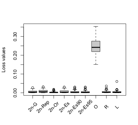
(a) $\tau=10^{-4}$

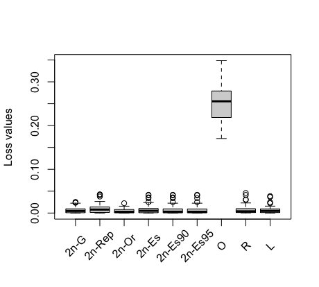
(b) $\tau=10^{-2}$

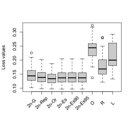
(c) $\tau=1$

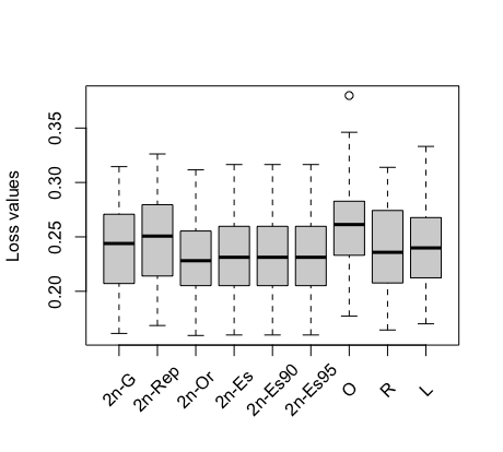
(d) $\tau=10^{0.5}$

(e) $\tau=10^{-4}$

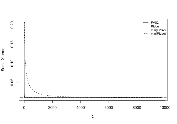
(f) $\tau=10^{-2}$

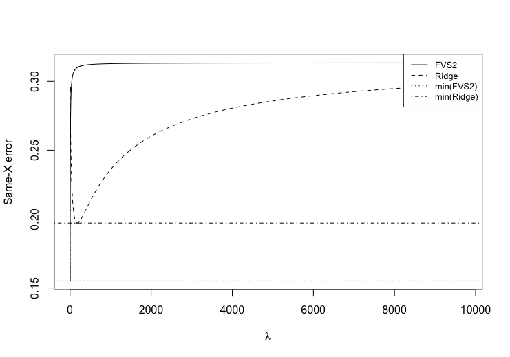
(g) $\tau=1$

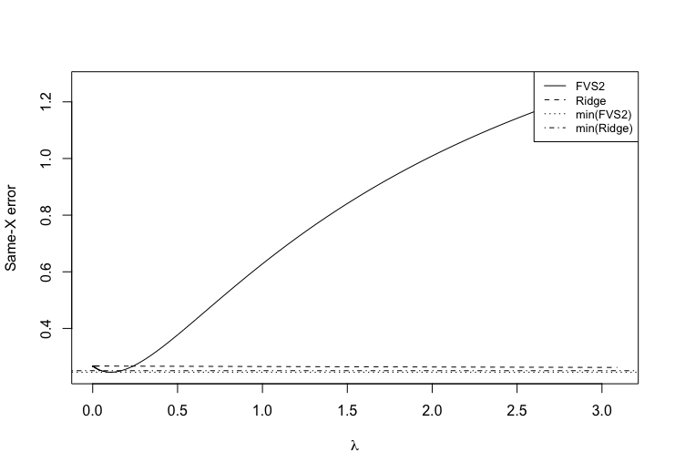
(h) $\tau=10^{0.5}$

Figure 1: Boxplots of the observed same-X loss values from the 50 replications (a–d) and graphs of the average same-X loss values over the 50 replications as a function of $\lambda$ comparing our proposed method (2) to Ridge (22) (e–h) when $n=300$ and $p=75$. The label FVS2 is fitted value shrinkage with $L_{2}$-squared penalty (2), and the vertical lines, min(FVS2) and min(Ridge), are the minimal average same-X loss values obtained from each estimator within the set of $\lambda$.

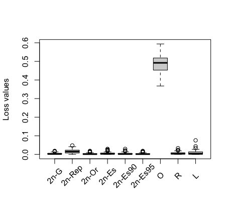
(a) $\tau=10^{-4}$

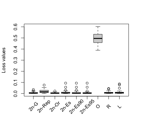
(b) $\tau=10^{-2}$

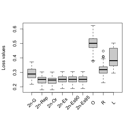
(c) $\tau=1$

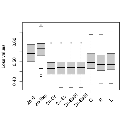
(d) $\tau=10^{0.5}$

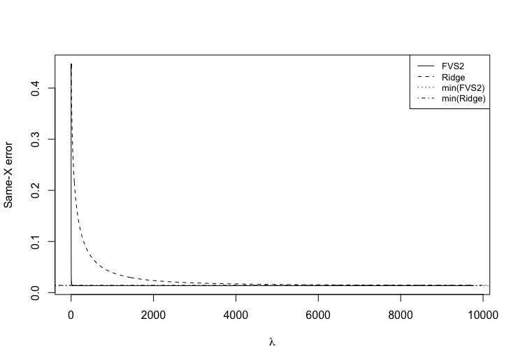
(e) $\tau=10^{-4}$

(f) $\tau=10^{-2}$

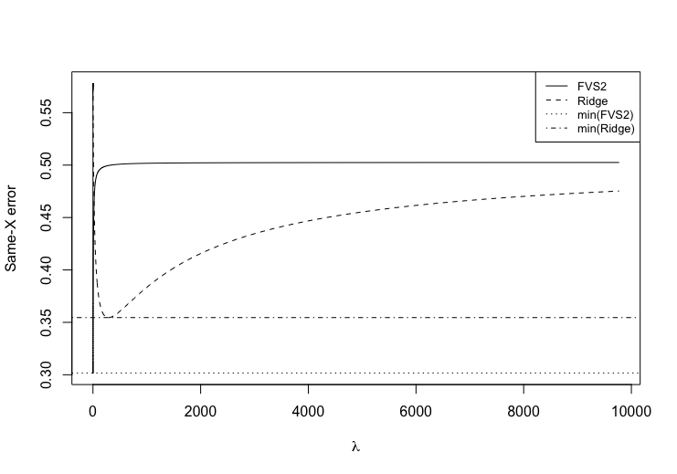
(g) $\tau=1$

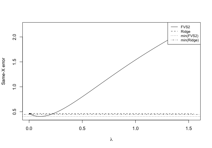
(h) $\tau=10^{0.5}$

Figure 2: Boxplots of the observed same-X loss values from the 50 replications (a–d) and graphs of the average same-X loss values over the 50 replications as a function of $\lambda$ comparing our proposed method (2) to Ridge (22) (e–h) when $n=300$ and $p=150$. See the caption of Figure 1 for more details.

6.2 High-dimensional experiments

We used the same data generating model as in Section 6.1 except that $n=200$, $p=300$, and $\sigma\in\{2,3\}$. Since 2n-Es is not applicable in high dimensions, we tested variants of 2n-G that used 5, 10, and $n$-fold cross validation. They are labeled 2n-5fold, 2n-10fold, 2n-Loocv, respectively. In addition, we tried different $\alpha$ values that control the matrix $K$ in (16) for the following variants of 2n-Rep:

• 2n-Rep1: Same as original 2n-Rep with $\alpha=n(2\|Y-P_{1}Y\|^{2})^{-1}$.

• 2n-Rep2: $\bar{\gamma}_{c}$ (16) using $\check{\sigma}^{2}$ with $\alpha=n^{3/2}(2\|Y-P_{1}Y\|^{2})^{-1}$.

• 2n-Rep3: Same as original 2n-Rep with $\alpha=n^{2}(2\|Y-P_{1}Y\|^{2})^{-1}$.

• 2n-Rep4: Same as original 2n-Rep with $\alpha=n^{3}(2\|Y-P_{1}Y\|^{2})^{-1}$.

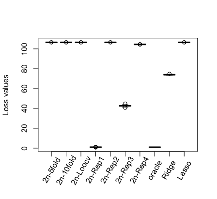
(a) $(1,10)$

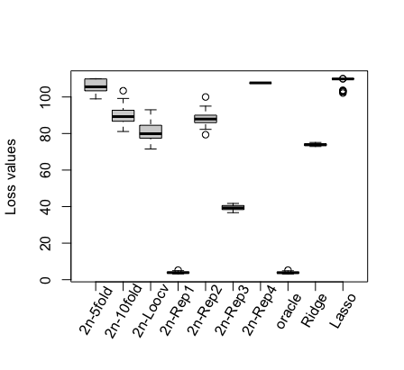
(b) $(2,10)$

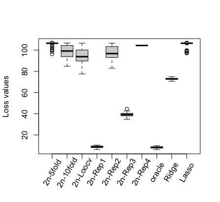
(c) $(3,10)$

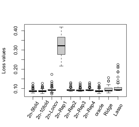
(d) $(1,10^{-0.5})$

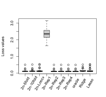
(e) $(2,10^{-0.5})$

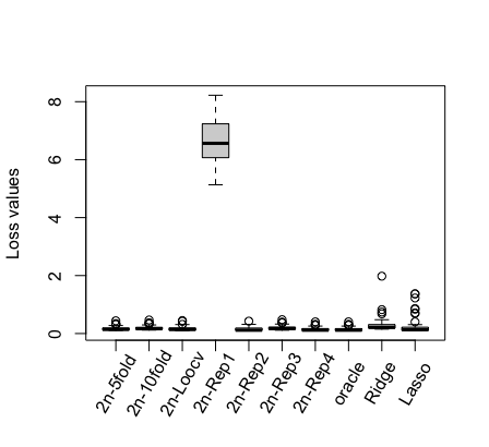
(f) $(3,10^{-0.5})$

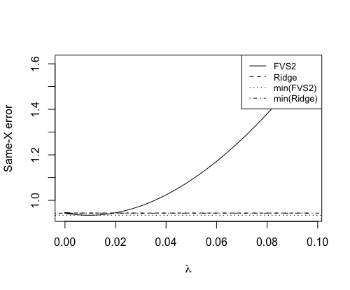
(g) $(1,10)$

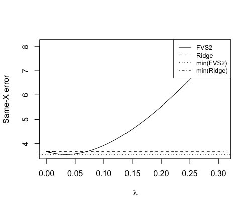
(h) $(2,10)$

(i) $(3,10)$

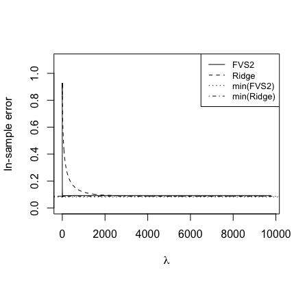
(j) $(1,10^{-0.5})$

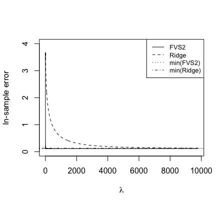
(k) $(2,10^{-0.5})$

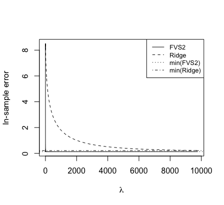
(l) $(3,10^{-0.5})$

Figure 6: Additional displays to Figure 3, and 4. Boxplots of the observed same-X loss values from the 50 replications (a–f) and graphs of the average same-X loss values over the 50 replications as a function of $\lambda$ comparing our proposed method (2) to Ridge (22) (g–l) when $(n,p)=(200,300)$.

In Figure 3, we display side-by-side boxplots of the observed same-X losses from the 50 replications when $n=200$ and $p=300$. There are additional boxplots displayed in Figure 6 in Appendix A.6. In general, when $\delta^{2}=\|\mu-P_{1}\mu\|^{2}$ is large relative to $n\sigma^{2}$, which corresponds to the situation $\gamma_{\rm opt}\rightarrow 1$, 2n-Rep1 performs better than Ridge, Lasso, 2n-Gs, and 2n-Rep2 to 2n-Rep4 (Figure 3(a), 3(f)). Furthermore, larger $\delta^{2}$ led to improved tuning-parameter selection (Figure 3(d), 6(a), 3(e), 6(b), 6(c)). In these situations, Ridge, Lasso, and 2n-Gs, and other variants of 2n-Reps performed poorly. However, 2n-Gs, Ridge, and Lasso performed better when $\delta^{2}$ is small relative to $n\sigma^{2}$. In this setting, which can be identified with $\gamma_{\rm opt}\rightarrow 0$, 2n-Rep2, 2n-Rep3, and 2n-Rep4 performed at least comparable to or even better than Ridge, Lasso, and 2n-Gs (see Figure 3(b), 3(c), 6(d), 6(e), 6(f)). On the other hand, 2n-Rep1 struggled for this case. Except for a few cases, the number of folds used for tuning parameter selection for 2n-G did not have a significant impact on the prediction accuracy.

In Figure 4, we display average loss values over the 50 replications as a function of $\lambda$ when $n=200$ and $p=300$. These results look similar to lower-dimensional results displayed in Figure 1, except the curve valleys are narrower for fitted-value shrinkage.

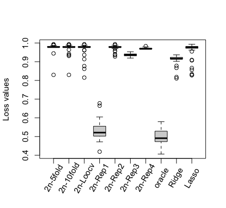
(a) $(1,1)$

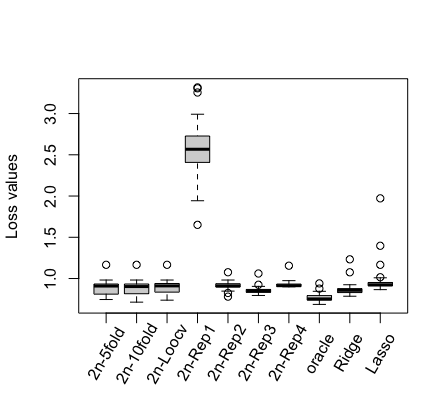
(b) $(2,1)$

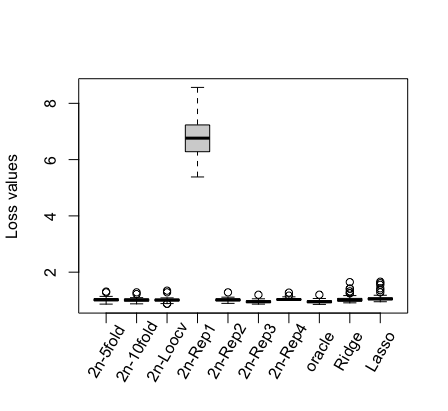
(c) $(3,1)$

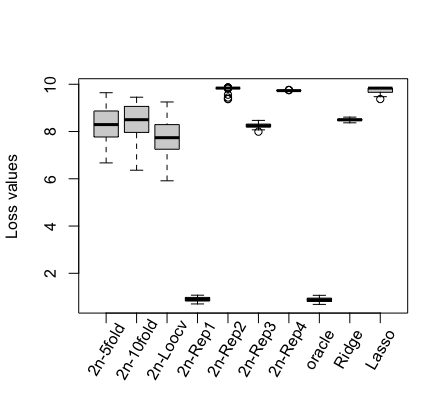
(d) $(1,10^{0.5})$

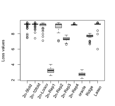
(e) $(2,10^{0.5})$

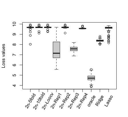
(f) $(3,10^{0.5})$

Figure 3: Boxplots of the observed same-X loss values from the 50 replications when $(n,p)=(200,300)$. Each plot is labeled with the $(\sigma,\tau)$ value used.

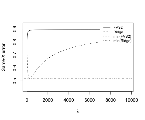
(a) $(1,1)$

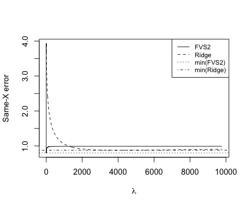
(b) $(2,1)$

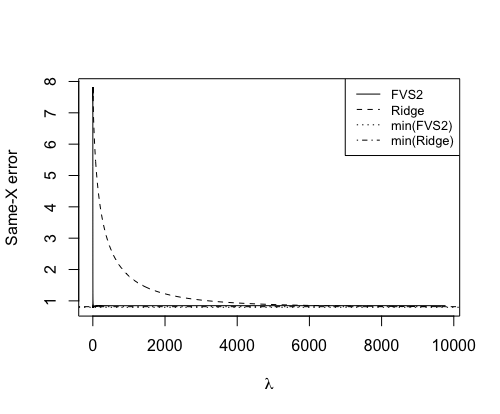
(c) $(3,1)$

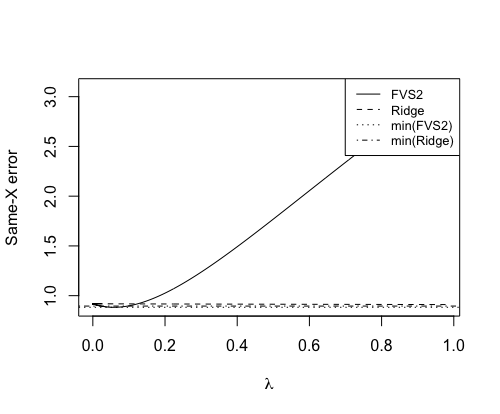
(d) $(1,10^{0.5})$

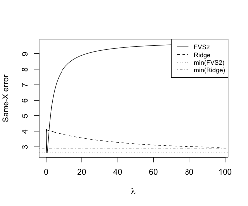
(e) $(2,10^{0.5})$

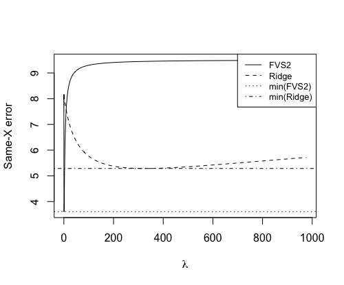
(f) $(3,10^{0.5})$

Figure 4: Graphs of the average same-X loss values over the 50 replications as a function of $\lambda$ comparing our proposed method (2) to Ridge (22) when $(n,p)=(200,300)$. Each plot is labeled with the $(\sigma,\tau)$ value used.

7 Data examples

7.1 Low dimensional data experiments

We compared our proposed fitted-value shrinkage procedures to competitors on three data sets. We used the same non-oracle estimators as the previous section except we excluded 2n-Es90 because it performed similarly to 2n-Es95. Each data example was analyzed using the following procedure: For 50 independent replications, we randomly selected 70% of the subjects for the training set and used the remaining subjects as the test set. Tuning parameter selection was done using the training set and prediction performance was measured using squared error loss on the test set. The following is the short description of the three low-dimensional data set we examined.

1. : The Forest Fire (FF) data are from from Cortez and Morais (2007) and are stored at the UCI Machine learning repository via https://archive.ics.uci.edu/dataset/162/forest+fires. There are 517 observations corresponding to forest fires in Portugal from 2000 to 2003. The response is the total burned area (in $ha$) from the fire, which was transformed with $x\mapsto{\rm ln}(x+1)$, which was suggested by Cortez and Morais (2007). There were originally 13 attributes. However, in the pre-processing step, since we are not focusing on spatio-temporal methods, we excluded time, date and location coordinates. After this processing, the full-data design matrix had $(n,p)=(517,9)$ with 8 numerical-variable columns and one intercept column.

2. : The GDP data (GDP) are from Barro and Lee (1994). These data consist of 161 observations of GDP growth rates for the two periods 1965-1975 and 1975-1985. The data are also in the R package quantreg (Koenker, 2022). The response is Annual change per capita GDP. There are 13 numerical predictors, e.g. Initial per capita GDP, Life expectancy. We also added a quadratic term for the predictor Black Market Premium. After processing, the full-data design matrix has $(n,p)=(161,15)$.

3. : The Forecast data set (FC) is from Cho et al. (2020) for the purpose of bias correction for the Local Data Assimilation and Prediction System (LDAPS), which is a numerical weather report model used by Korea Administration (KMA), Seoul, South Korea. It has a public access through https://archive.ics.uci.edu/dataset/514/bias+correction+of+numerical+prediction+model+temperature+forecast. The data are regional observations from 2013 to 2017, from which we randomly selected 500. We used the true maximal temperature of the next day as the response and removed date, station ID, and true minimal temperature of the next day. The full-data design matrix had $(n,p)=(500,20)$.

In Table 1, we display mean squared prediction errors averaged over 50 training/test set splits for the three data examples (FF), (GDP), and (FC). Our fitted-value shrinkage estimators performed similarly to Ridge and Lasso, which both lack invariance to invertible linear transformations of the design matrix.

Performance comparison table
Data set	2n-Rep	2n-G	2n-Es	2n-Es95	OLS	Ridge	LASSO
Forest Fire	2.0016	2.0160	2.0017	1.9857	2.1834	2.0189	2.0572
(FF)	(0.0275)	(0.0316)	(0.0300)	(0.0269)	(0.0551)	(0.0322)	(0.0411)
GDP growth	3.328e-04	3.125e-04	3.139e-04	3.314e-04	3.231e-04	3.112e-04	3.149e-04
(GDP)	(7.533e-06)	(7.615e-06)	(7.706e-06)	(8.055e-06)	(8.120e-06)	(8.126e-06)	(8.307e-06)
Forecast	1.8635	1.8997	1.9028	1.8531	2.0489	1.8990	1.8978
(FC)	(0.0345)	(0.0325)	(0.0327)	(0.0345)	(0.0371)	(0.0321)	(0.0318)

Table 1: The performance comparison table for three data examples in Section 7.1. The values are the mean squared prediction errors averaged over 50 training/test set splits. The numbers in parentheses are normalized sample standard deviations. The column labels are defined in Section 6.1.

7.2 Low dimensional data analyses with categorical variables and their interactions

We analyzed two data sets from existing R packages to illustrate the performance of our estimators when categorical variables with interactions are present in the model. The competitors and setup for the data experiments are nearly identical to the previous Section 7.1, except we added three new fitted-value shrinkage estimators that shrink toward the submodel without interactions instead of the intercept-only model and Group Lasso and its two variants. These new submodel shrinkage methods are labeled 2n-Repsb, 2n-Gsb, 2n-Essb, 2n-Es95sb, and they respectively correspond to 2n-Rep, 2n-G, 2n-Es, and 2n-Es95. We specify the Group lasso competitors as the following:

• GL: Group Lasso estimator proposed by Yuan and Lin (2006).

  $$\hat{\beta}_{\rm GL}=\operatorname*{arg\ min}_{b\in\mathbb{R}^{p}}\|Y-Xb\|^{2}+\lambda\sum_{i=1}^{L}\sqrt{p_{i}}\|b^{(i)}\|_{2},$$

  where $i\in\{1,\ldots,L\}$ is the index of each group except for one intercept column; $p_{i}$ is the size of the $i$-th group; and $b^{(i)}$ is the corresponding subvector.

• MGL: Modified Group Lasso proposed by Choi et al. (2012).

  $$\hat{\beta}_{\rm MGL}=\operatorname*{arg\ min}_{b\in\mathbb{R}^{p}}\|Y-Xb\|^{2}+\lambda\sum_{i=1}^{L}\|b^{(i)}\|_{2}.$$

• SGL: Standardized Group Lasso proposed by Simon and Tibshirani (2012).

  $$\hat{\beta}_{\rm SGL}=\operatorname*{arg\ min}_{b\in\mathbb{R}^{p}}\|Y-Xb\|^{2}+\lambda\sum_{i=1}^{L}\sqrt{p_{i}}\|X^{(i)}b^{(i)}\|_{2},$$

  where $X^{(i)}$ is the $i$-th submatrix.

The following is a description of the data examples:

1. : The Diamonds data set is from Diamonds data frame in the R package Stat2Data (Cannon et al., 2019), and it was obtained from https://awesomegems.com/. The are $n=351$ subjects and the response is the price of the diamond (in dollars). We divided price per 1000 and used it for the response variable. We further removed total price from the predictors. There are 2 categorical predictors: color (with levels D to J) and clarity (with levels IF, VVS1, VVS2, VS1, VS2, SI1, SI2, and SI3). We divided color into 5 levels (D, E, F, G, and (H,I,J)), and categorized the clarity into 3 levels ((IF, VVS1, VVS2), (VS1, VS2), (SI1, SI2, SI3)). We used reference-level coding in the design matrix, where (H,I,J) was the reference level for color; and (SI1, SI2, SI3) was the reference level for clarity. Interactions between color and depth as well as clarity and depth were added. The full design matrix has $(n,p)=(351,15)$ and the submodel with linear terms only has $p=9$.

2. : The setting is identical to that of (Dia-1), except we used the category (VS1, VS2) as the reference level for coding the categorical predictor clarity.

3. : The NaturalGas data is from Baltagi (2002), and is in the R package AER (Kleiber and Zeileis, 2008). There are 138 observations on 10 variables. We removed state name and year and added an interaction between state code and heating degree days. We set the response as consumption divided by 10000. The reference level for state code, which is the only categorical predictor, was set to 35 (NY). The full-data design matrix had $(n,p)=(138,17)$ and the submodel without interactions had $p=12$.

4. : This is the same as (NG-1), except the reference level for state code was set to 5 (CA).

We display mean squared prediction errors averaged over 50 training/test set splits for these data examples in Table 2. Our proposed estimators performed similarly or better than Ridge and Lasso. We also notice that changing the way that categorical predictors were encoded in the design matrix changes the performance of Ridge and Lasso, which lack invariance. Furthermore, Group Lasso and its two standardized versions had unstable performance when the base level coding was changed, which does not happen to our invariant methods.

Performance comparison table
Data set	2n-Rep	2n-Repsb	2n-G	2n-Gsb	2n-Es	2n-Essb	2n-Es95	2n-Es95sb	OLS	Ridge	LASSO	GL	MGL	SGL
Diamonds	1.2538	1.2557	1.2545	1.2501	1.2557	1.2507	1.2557	1.2599	1.2587	1.2668	1.2675	1.2699	1.2693	1.2603
(Dia-1)	(0.0303)	(0.0300)	(0.0298)	(0.0293)	(0.0295)	(0.0294)	(0.0295)	(0.0294)	(0.0293)	(0.0297)	(0.0297)	(0.0290)	(0.0290)	(0.0301)
Diamonds	1.2538	1.2557	1.2545	1.2501	1.2557	1.2507	1.2557	1.2599	1.2587	1.2615	1.2624	1.2697	1.2693	1.2582
(Dia-2)	(0.0303)	(0.0300)	(0.0298)	(0.0293)	(0.0295)	(0.0294)	(0.0295)	(0.0294)	(0.0293)	(0.0296)	(0.0299)	(0.0286)	(0.0287)	(0.0297)
Natural gas	5.2558	5.2485	5.2899	5.2711	5.2559	5.2523	5.2559	5.2523	5.2545	5.2913	5.1254	5.2972	5.3010	5.2078
(NG-1)	(0.2285)	(0.2262)	(0.2282)	(0.2217)	(0.2285)	(0.2257)	(0.2285)	(0.2257)	(0.2279)	(0.2195)	(0.2285)	(0.2241)	(0.2242)	(0.2271)
Natural gas	5.2558	5.2486	5.2899	5.2711	5.2559	5.2523	5.2559	5.2523	5.2545	5.3563	5.2889	5.2261	5.2010	7.0627
(NG-2)	(0.2285)	(0.2262)	(0.2282)	(0.2217)	(0.2285)	(0.2257)	(0.2285)	(0.2257)	(0.2279)	(0.2195)	(0.2285)	(0.2171)	(0.2168)	(0.2816)

Table 2: The performance comparison table for two data sets in Section 7.2 with two different coding strategies. The values are mean squared prediction errors averaged over 50 training/test splits. The numbers in parentheses are normalized sample standard deviations. The labels are defined in Section 6.1 except that last three are illustrated in Section 7.2. The suffix ”sb” for each estimator corresponds to shrinking towards the submodel without interactions instead of shrinking towards the intercept-only model (see Section 5 for details).

7.3 High dimensional data experiments

For high-dimensional data examples, we randomly selected subjects from existing data sets so that there were fewer subjects than predictors. We used the same splitting and evaluation procedure that we used in Sections 7.1 and 7.2. The competitors are same as those considered in Section 6.2 except that we excluded 2n-Rep4 which had nearly identical performance to 2n-Rep3 in the simulation study. The following is a description of the examples:

1. : The data set mtp comes from Karthikeyan et al. (2005) and is available at the OpenML repository via https://www.openml.org/search?type=data&status=active&id=405. There are 4450 subjects with 203 numerical measurements. The response is oz203. We randomly selected 120 subjects and removed the 23 predictors that had fewer than 30 distinct values, which ensured that there were no constant columns in the 120-row design matrix other than the intercept column. The full-data design matrix had $(n,p)=(120,180)$.

2. : The topo.2.1 data set is from Feng et al. (2003) and is available through the OpenML repository via https://www.openml.org/search?type=data&sort=runs&id=422&status=active. There are 8885 subjects with 267 numerical measurements. The response is oz267. We randomly selected 180 subjects and removed the 22 predictors that had fewer than 30 distinct values. After this, there were 34 constant columns (other than the intercept) that were also removed. The R code for this processing is in Appendix A.7.1. The full-data design matrix has $(n,p)=(180,214)$.

3. : The tecator data set comes from Thodberg (2015), and is also available from OpenML repository via https://www.openml.org/search?type=data&status=active&sort=runs&order=desc&id=505. We randomly selected 100 subjects and removed 22 principal components. The response is fat content. The full-data design matrix had $(n,p)=(100,103)$.

In Table 3, we report the mean squared prediction errors averaged over 50 training/test set splits for these data examples. We see that 2n-Rep2, 2n-Rep3, 2n-Rep4 had similar prediction performance compared to 2n-Rep1. In contrast to its same-X loss performance in simulations, the cross validation version of our method 2n-G gave reasonable out-of-sample prediction performance. Generally, 2n-Rep1 and 2n-Rep2 performed competitively compared with Ridge and Lasso, and 2n-Rep3 followed the next within 2n-Reps.

Performance comparison table
Data set	OLS	2n-G	Ridge	LASSO	2n-Rep1	2n-Rep2	2n-Rep3
mtp	0.5075	0.0266	0.0262	0.0227	0.0264	0.0266	0.0264
(mtp)	(0.0592)	(0.0010)	(0.0027)	(0.0017)	(0.0008)	(0.0008)	(0.0008)
topo.2.1	0.07524	0.00085	0.00096	0.00087	0.00086	0.00085	0.00086
(topo)	(2.72e-02)	(2.75e-05)	(7.71e-05)	(3.27e-05)	(2.15e-05)	(2.08e-05)	(2.15e-05)
tecator	2.4400	2.4592	2.7251	2.7120	2.4266	2.4316	2.4733
(tecator)	(0.2359)	(0.2348)	(0.1913)	(0.1940)	(0.2202)	(0.2188)	(0.2148)

Table 3: The performance comparison table for three high dimensional real data sets in Section 7.3. The values are mean squared prediction errors averaged over 50 replications. The numbers in parentheses are normalized sample standard deviations. The labels are defined in Section 6.2.

8 Future directions

The fitted-value shrinkage idea presented here to fit linear regression models with invariance can be extended to more complicated settings. For example, one could fit a logistic regression model by minimizing the negative loglikelihood plus the penalty $\lambda\|X\beta-\hat{w}1_{n}\|^{2}$, where $\hat{w}$ is the sample log-odds that the response takes its first category. We are currently developing this procedure.

A Bayesian formulation of our method may also be interesting. In addition, one could study methods that combine our proposed invariant shrinkage penalty with regular shrinkage penalties like the lasso or ridge.

Supplementary material for Fitted value shrinkage

Appendix A Appendix

A.1 Proof of Proposition 1

Proof.

We start with the following standard decomposition:

$$\mathbb{E}\|X\hat{\beta}^{(\gamma)}-X\beta\|^{2}={\rm tr}\Big{(}{\rm var}\Big{(}X\hat{\beta}^{(\gamma)}-X\beta\Big{)}\Big{)}+\Big{\|}\mathbb{E}\Big{(}X\hat{\beta}^{(\gamma)}-X\beta\Big{)}\Big{\|}^{2}.$$

From (4),

$${\rm tr}\Big{(}{\rm var}\Big{(}X\hat{\beta}^{(\gamma)}-X\beta\Big{)}\Big{)} ={\rm tr}\Big{(}\sigma^{2}\Big{(}\gamma^{2}P_{X}+(1-\gamma^{2})P_{1}\Big{)}\Big{)},$$

$$=\sigma^{2}(\gamma^{2}r+1-\gamma^{2})$$

$$\mathbb{E}\Big{(}X\hat{\beta}^{(\gamma)}-X\beta\Big{)} =(1-\gamma)(\mu-P_{1}\mu),$$

where $\mu=X\beta$. Combining above two equations, we conclude that the statement holds. ∎

A.2 Proof of Proposition 2

Lemma 1.

When a $n$-variate random variable $V=(V_{1},\dots,V_{n})$ has i.i.d. elements $V_{i}$ following a distribution that has mean $\mu$, variance $\sigma^{2}$, and has finite $4$-th moment with $\mathbb{E}(V_{i}^{4})\leq M$, for all $i=1,\dots,n$. Let an $(i,j)$-th element of $A$ be $a_{ij}$, then, for a symmetric non-negative definite $A\in\mathbb{R}^{n\times n}$,

$${\rm var}(V^{\prime}AV)\leq 2(M-3\sigma^{4})\sum_{i=1}^{n}a_{ii}^{2}+4\sigma^{4}{\rm tr}(A^{2})+8\sigma^{2}\mu^{\prime}A^{2}\mu$$

holds.

Proof.

For the simplest case, we first consider when $\mu=0$. Then, by the i.i.d property of $\{V_{i}\}$ and the moment conditions,

$$\mathbb{E}\Big{[}(V^{\prime}AV)^{2}\Big{]} \leq M\sum_{i=1}^{n}a_{ii}^{2}+\sigma^{4}\sum\sum_{1\leq i\neq j\leq n}a_{ii}a_{jj}+2\sigma^{4}\sum\sum_{1\leq i\neq j\leq n}a_{ij}a_{ji}$$

$$=M\sum_{i=1}^{n}a_{ii}^{2}+\sigma^{4}\Big{(}({\rm tr}(A))^{2}-\sum_{i=1}^{n}a_{ii}^{2}\Big{)}+2\sigma^{4}\Big{(}{\rm tr}(A^{2})-\sum_{i=1}^{n}a_{ii}^{2}\Big{)}$$

$$=(M-3\sigma^{4})\sum_{i=1}^{n}a_{ii}^{2}+\sigma^{4}\Big{(}({\rm tr}(A))^{2}+2{\rm tr}(A^{2})\Big{)}$$

Together with, $\mathbb{E}(V^{\prime}AV)=\sigma^{2}{\rm tr}(A)$, we know that,

$${\rm var}\Big{[}(V^{\prime}AV)^{2}\Big{]}=(M-3\sigma^{4})\sum_{i=1}^{n}a_{ii}^{2}+2\sigma^{4}{\rm tr}(A^{2})$$

For general $V$ with $\mu\neq 0$, we denote $V=V_{0}+\mu$, then,

$${\rm var}(V^{\prime}AV) ={\rm var}(V_{0}^{\prime}AV_{0}+2\mu^{\prime}AV_{0})$$

$$\leq 2{\rm var}(V_{0}^{\prime}AV_{0})+8{\rm var}(\mu^{\prime}AV_{0}).$$

This completes the proof. ∎

Now we turn to the proof of Proposition 2.

Proof.

Let $\delta^{2}=\|\mu-P_{1}\mu\|^{2}$ and define $A_{n}=\|P_{X}Y-P_{1}Y\|^{2}/(r-1),B_{n}=\|Y-P_{X}Y\|^{2}/(n-r)$ and their expected values $a_{n}=\sigma^{2}+{\delta^{2}}/({r-1}),b_{n}=\sigma^{2}$, respectively. Then we can express $\gamma_{\rm opt}=1-{1}/{f_{n}}$ with its sample counterpart $1-{1}/{F_{n}}$ where $F_{n}={A_{n}}/{B_{n}},f_{n}={a_{n}}/{b_{n}}$. At first glance, considering that

$$f_{n}=\frac{a_{n}}{b_{n}}=1+\frac{\delta^{2}}{\sigma^{2}({\rm rank}(X)-1)},$$

it is obvious that $f_{n}\geq 1$. By the assumption, we have the error distribution to be $\mathbb{E}(e_{i}^{4})\leq M$, for $M>0,i=1,\dots,n$.

For the first step, knowing that $\mathbb{E}(B_{n})=b_{n}$,

$$\mathbb{E}(B_{n}-b_{n}) =0$$

$${\rm var}(B_{n}-b_{n}) ={\rm var}(B_{n})$$

$$=\frac{1}{(n-r)^{2}}{\rm var}\|(I-P_{X})Y\|^{2}$$

$$=\frac{1}{(n-r)^{2}}{\rm var}\left\{Y^{\prime}(I-P_{X})Y\right\}$$

$$\leq\frac{2(M-\sigma^{4})}{n-r},$$

which converges to 0 because $n\rightarrow\infty$ and $r/n\rightarrow\tau\in[0,1)$. The last inequality is due to Lemma 1, with the fact that $I-P_{X}$ is an idempotent matrix with rank $n-r$.

So $B_{n}-b_{n}\rightarrow_{q.m}0$, which implies that $B_{n}/b_{n}\rightarrow_{q.m.}1$ because $b_{n}=\sigma^{2}$ is constant.

Next, knowing that $\mathbb{E}(A_{n})=a_{n}$, similarly,

$$\mathbb{E}\Big{(}\frac{A_{n}}{a_{n}}-1\Big{)} =0$$

$${\rm var}\Big{(}\frac{A_{n}}{a_{n}}-1\Big{)} =\frac{1}{a_{n}^{2}}{\rm var}(A_{n})$$

$$=\frac{1}{a_{n}^{2}(r-1)^{2}}{\rm var}\left\{\|(P_{X}-P_{1})Y\|^{2}\right\}$$

$$=\frac{1}{a_{n}^{2}(r-1)^{2}}{\rm var}\left\{Y^{\prime}(P_{X}-P_{1})Y\right\}$$

$$\leq\frac{2(M-\sigma^{4})(r-1)+8\delta^{2}\sigma^{2}}{(\sigma^{2}(r-1)+\delta^{2})^{2}}$$ (24)

$$=\frac{2(M-\sigma^{4})(r-1)+8\delta^{2}\sigma^{2}}{\sigma^{4}(r-1)^{2}+\delta^{4}+2\sigma^{2}\delta^{2}(r-1)},$$ (25)

where we used Lemma 1 for (24) with the fact that $P_{X}-P_{1}$ is an idempotent matrix with rank $r-1$. If $r\rightarrow\infty$ holds, since (25) is bounded above by $4(r-1)^{-1}+{2(M-\sigma^{4})}({\sigma^{4}(r-1)})^{-1}$, it converges to $0$.

On the other hand, under the second condition, we have the same convergence result. This is because we can have an upper bound of (25) as $({M-\sigma^{4}})({2\sigma^{2}\delta^{2}})^{-1}+{8\sigma^{2}}({\delta^{2}})^{-1}$, it converges to $0$ with $\delta^{2}\rightarrow\infty$.

Combining two convergence results, $B_{n}/b_{n}\rightarrow_{q.m}1,A_{n}/a_{n}\rightarrow_{q.m}1$, it implies $B_{n}/b_{n}\rightarrow_{p}1,A_{n}/a_{n}\rightarrow_{p}1$, and further yields $F_{n}/f_{n}=\frac{A_{n}/a_{n}}{B_{n}/b_{n}}\rightarrow_{p}1$ by Slutsky’s theorem.

Additionally, let us denote that $F^{0}_{n}={\rm max}(1,F_{n})$, then we have $\hat{\gamma}=1-{1}/{F^{0}_{n}}$. Finally, we get

$$\mathbb{P}(|\hat{\gamma}-\gamma_{\rm opt}|\geq\epsilon) =\mathbb{P}\Big{(}\Big{|}1-\frac{1}{F^{0}_{n}}-1+\frac{1}{f_{n}}\Big{|}\geq\epsilon\Big{)}$$

$$=\mathbb{P}\Big{(}\Big{|}\frac{1}{F^{0}_{n}}-\frac{1}{f_{n}}\Big{|}\geq\epsilon\Big{)}$$

$$=\mathbb{P}\Big{(}\frac{|F^{0}_{n}-f_{n}|}{F^{0}_{n}f_{n}}\geq\epsilon\Big{)}$$

$$\leq\mathbb{P}\Big{(}\frac{|F_{n}-f_{n}|}{F_{n}f_{n}}\geq\epsilon,F_{n}\geq 1\Big{)}+\mathbb{P}\Big{(}{|1-f_{n}|}\geq\epsilon,F_{n}<1\Big{)}$$

$$\leq\mathbb{P}\Big{(}\frac{|F_{n}-f_{n}|}{f_{n}}\geq\epsilon,F_{n}\geq 1\Big{)}+\mathbb{P}\Big{(}f_{n}\geq 1+\epsilon,F_{n}<1\Big{)}$$

$$\leq\mathbb{P}\Big{(}\Big{|}\frac{F_{n}}{f_{n}}-1\Big{|}\geq\epsilon\Big{)}+\mathbb{P}\Big{(}\Big{|}\frac{F_{n}}{f_{n}}-1\Big{|}\geq\frac{\epsilon}{1+\epsilon}\Big{)}\rightarrow 0.$$

∎

A.3 Proof of Proposition 3

Lemma 2.

If a random variable $X$ follows a chi-squared distribution with a degree of freedom $K\geq 5$, and a non-central parameter $\lambda>0$ which is denoted as $\chi^{2}(K;\lambda)$, the followings holds.

$$\mathbb{E}(X^{-1})\leq{\rm min}\Big{\{}\frac{1}{K-2},\frac{1}{2\sqrt{\lambda(K-2)}}\Big{\}}$$ (26)

$$\mathbb{E}(X^{-2})\leq{\rm min}\Big{\{}\frac{1}{2(K-4)},\frac{(K-4+\lambda)/(2\sqrt{\lambda(K-4)})-1}{2\lambda}\Big{\}}$$ (27)

Proof.

Xie (1988) verified the following three results for $K\geq 5$.

$$\mathbb{E}^{1}_{K}=\int_{0}^{1}s^{K-3}e^{\frac{\lambda(s^{2}-1)}{2}}ds,$$

$$\mathbb{E}^{1}_{K}=1/\lambda-((K-4)/\lambda)\mathbb{E}^{1}_{K-2},$$

$$\mathbb{E}^{n}_{K}-\mathbb{E}^{n}_{K+2}=2n\mathbb{E}^{n+1}_{K+2},$$

where $\mathbb{E}^{n}_{K}=\mathbb{E}(1/(\chi^{2}(K;\lambda))^{n})$. Hence

$$\mathbb{E}(X^{-2})=\mathbb{E}^{2}_{K} =\frac{\mathbb{E}^{1}_{K-2}-\mathbb{E}^{1}_{K}}{2}$$

$$=\frac{(K-4+\lambda)\mathbb{E}^{1}_{K-2}-1}{2\lambda}$$

holds. Furthermore,

$$\mathbb{E}(X^{-1})=\mathbb{E}^{1}_{K} =\int_{0}^{1}s^{K-3}e^{\frac{\lambda(s^{2}-1)}{2}}ds$$

$$\leq\int_{0}^{1}s^{K-3}ds=\frac{1}{K-2}.$$

On the other hand, from the same equation,

$$\int_{0}^{1}s^{K-3}e^{\frac{\lambda(s^{2}-1)}{2}}ds$$

$$\leq e^{-\lambda/2}\Big{(}\int_{0}^{1}s^{2K-5}ds\Big{)}^{1/2}\Big{(}\int_{0}^{1}se^{\lambda s^{2}}ds\Big{)}^{1/2}$$

$$=e^{-\lambda/2}\frac{1}{\sqrt{2K-4}}\frac{\sqrt{e^{\lambda}-1}}{\sqrt{2\lambda}}$$

$$\leq\frac{1}{2\sqrt{\lambda(K-2)}}.$$

This completes the proof. ∎

With Lemma 2, we prove the statement of Proposition 3.

Proof.

From the definition of $\hat{\gamma}$ (4), we obtain

$$|\hat{\gamma}-\gamma_{\rm opt}| =\Big{|}I(F_{n}\geq 1)(1-1/F_{n})-(1-1/f_{n})\Big{|}$$

$$\leq\Big{|}\frac{1}{f_{n}}-\frac{1}{F_{n}}\Big{|},$$ (28)

where $\gamma_{\rm opt}=1-1/f_{n}$, $f_{n}=\frac{\sigma^{2}(r-1)+\delta^{2}}{\sigma^{2}(r-1)}=1+\frac{\delta^{2}}{\sigma^{2}(r-1)}\in[1,\infty)$.

Let us follow the same notations in Proposition 2 as $F_{n}={A_{n}}/{B_{n}},f_{n}={a_{n}}/{b_{n}}$, where $A_{n}=\|P_{X}Y-P_{1}Y\|^{2}/(r-1),B_{n}=\|Y-P_{X}Y\|^{2}/(n-r),a_{n}=\sigma^{2}+{\delta^{2}}/({r-1}),b_{n}=\sigma^{2}$. Since we have normal errors, $A_{n},B_{n}$ are independent. In addition, $(r-1)A_{n}/\sigma^{2}\sim\chi^{2}(r-1;\delta^{2}/\sigma^{2})$, $(n-r)B_{n}/\sigma^{2}\sim\chi^{2}(n-r)$, and we denote $A^{\prime}_{n}:=A_{n}/\sigma^{2},B^{\prime}_{n}:=B_{n}/\sigma^{2}$. First, we consider the first case where $\delta^{2}=O(r)$. Since $F_{n}$ follows non-central $F$ distribution,

$$\mathbb{E}(F_{n}) =\frac{(n-r)(r-1+\delta^{2}/\sigma^{2})}{(r-1)(n-r-2)}$$

$$=\Big{(}\frac{2}{n-r-2}+1\Big{)}f_{n},$$

when $n-r>2$. And, with $n-r>4$,

$${\rm var}(F_{n})=2\frac{(n-r-2)(n-r)^{2}}{(n-r-4)(n-r-2)^{2}}\Big{[}\frac{(r-1+\delta^{2}/\sigma^{2})^{2}}{(n-r-2)(r-1)^{2}}+\frac{r-1+2\delta^{2}/\sigma^{2}}{(r-1)^{2}}\Big{]}.$$ (29)

Then,

$$\mathbb{E}(r(F_{n}-f_{n})^{2})=2r\frac{(n-r-2)(n-r)^{2}}{(n-r-4)(n-r-2)^{2}}\Big{[}\frac{(r-1+\delta^{2}/\sigma^{2})^{2}}{(n-r-2)(r-1)^{2}}+\frac{r-1+2\delta^{2}/\sigma^{2}}{(r-1)^{2}}\Big{]}+\frac{4r}{(n-r-2)^{2}}f_{n}^{2},$$

which asymptotically bounded by the assumptions. Furthermore, since we know that for arbitrary small $\epsilon>0$,

$$\hat{\gamma}-\gamma_{\rm opt}=-\gamma_{\rm opt}I(F_{n}\leq 1-\epsilon)+I(F_{n}\geq 1-\epsilon)(\hat{\gamma}-\gamma_{\rm opt})$$ (30)

holds, and the second term is bounded by (28). Indeed, on the event $F_{n}\geq 1-\epsilon$, by Cauchy-Schwarz inequality and the fact that $f_{n}\rightarrow f_{\infty}\in[1,\infty)$,

$$\Big{(}\mathbb{E}|1/f_{n}-1/F_{n}|\Big{)}^{2}\leq\frac{1}{f_{n}^{2}}\mathbb{E}|F_{n}-f_{n}|^{2}\mathbb{E}\Big{(}\frac{1}{F_{n}^{2}}\Big{)} \leq\frac{1}{(1-\epsilon)^{2}f_{n}^{2}}\mathbb{E}|F_{n}-f_{n}|^{2}\mathbb{E}\Big{(}\frac{1}{F_{n}^{2}}\Big{)}$$

$$\asymp\mathbb{E}|F_{n}-f_{n}|^{2}.$$

On the other hand, we show that the first term in (30) is negligible. Indeed, $P(F_{n}\leq 1-\epsilon)$ is at its largest when $f_{n}\rightarrow 1$, since $F_{n}/f_{n}\rightarrow 1$. Hence, it suffices to show that the tail bound of $P(F_{n}\leq 1-\epsilon)$ in the case of $f_{n}\rightarrow 1$ is negligible. Indeed,

$$P(F_{n}\leq 1-\epsilon) =P\Big{(}\frac{A^{\prime}_{n}}{B^{\prime}_{n}}\leq 1-\epsilon,A^{\prime}_{n}>1-\frac{\epsilon}{2}\Big{)}+P\Big{(}\frac{A^{\prime}_{n}}{B^{\prime}_{n}}\leq 1-\epsilon,A^{\prime}_{n}\leq 1-\frac{\epsilon}{2}\Big{)}$$

$$=P\Big{(}B^{\prime}_{n}\geq\frac{1-\frac{\epsilon}{2}}{1-\epsilon}\Big{)}+P\Big{(}A^{\prime}_{n}\leq 1-\frac{\epsilon}{2}\Big{)}.$$ (31)

Lemma 1 from Laurent and Massart (2000) with $x=nt/10$ yields $P(Z\geq 2nt)\leq{\rm exp}({-nt/10})$ for all $t\geq 1$, where a random variable $Z$ follows $\chi^{2}(n)$. This further implies that the first term in (31) is controlled by ${\rm exp}({-(n-r)(1-\frac{\epsilon}{2})/(20(1-\epsilon))})$ which has exponential decay in $n$. Furthermore, Theorem 7 of Zhang and Zhou (2020) yields that the second term in (31) is bounded above by ${\rm exp}({-\epsilon^{2}(r-1)^{2}/(16(r-1+\delta^{2}/\sigma^{2})}))$. Based on the case that $\delta^{2}=o(r)$, the upper bound has exponential decay in $r$. Consequently, $\mathbb{E}|1/f_{n}-1/F_{n}|=O(r^{-1/2})$ for $\delta^{2}=O(r)$.

However, when $r=o(\delta^{2})$, $f_{n}\rightarrow\infty$, hence the same reasoning cannot be applied. We use Lemma 2 instead. Indeed,

$$\mathbb{E}|1/f_{n}-1/F_{n}| =\mathbb{E}\Big{|}\frac{b_{n}A_{n}-B_{n}a_{n}}{A_{n}a_{n}}\Big{|}$$

$$\leq\mathbb{E}\frac{b_{n}}{A_{n}}\Big{|}\frac{A_{n}}{a_{n}}-1\Big{|}+\mathbb{E}\frac{1}{A_{n}}|B_{n}-b_{n}|$$

$$\leq\sigma^{2}\Big{[}\mathbb{E}\Big{(}\frac{A_{n}}{a_{n}}-1\Big{)}^{2}\mathbb{E}\Big{(}\frac{1}{A_{n}}\Big{)}^{2}\Big{]}^{1/2}+\Big{[}\mathbb{E}(B_{n}-b_{n})^{2}\Big{]}^{1/2}\mathbb{E}\Big{(}\frac{1}{A_{n}}\Big{)},$$

by Cauchy-Schwarz inequality and independence of $A_{n},B_{n}$. Since

$$\mathbb{E}\Big{(}\frac{1}{A_{n}}\Big{)}=\frac{(r-1)}{\sigma^{2}}\mathbb{E}(1/\chi^{2}(r-1;\delta^{2}))\leq\frac{(r-1)}{\sigma^{2}}{\rm min}\Big{\{}\frac{1}{r-3},\frac{1}{2\sqrt{\delta^{2}(r-3)}}\Big{\}}:=c_{1}(r,\delta^{2})/\sigma^{2},$$

and,

$$\mathbb{E}\Big{(}\frac{1}{A_{n}}\Big{)}^{2}=\frac{(r-1)^{2}}{\sigma^{4}}\mathbb{E}(1/\chi^{2}(r-1;\delta^{2}))^{2} \leq\frac{(r-1)^{2}}{\sigma^{4}}{\rm min}\Big{\{}\frac{1}{2(r-5)},\frac{(r-5+\delta^{2})/(2\sqrt{\delta^{2}(r-5)})-1}{2\delta^{2}}\Big{\}}$$

$$:=c_{2}(r,\delta^{2})/\sigma^{4}$$

from Lemma 2, and combining results from the Proposition 2,

$$\mathbb{E}|1/f_{n}-1/F_{n}|$$

$$\leq\frac{\sqrt{4\sigma^{4}(r-1)+8\delta^{2}\sigma^{2}}}{\sigma^{2}(r-1)+\delta^{2}}\sqrt{c_{2}(r,\delta^{2})}+\frac{\sqrt{2}}{\sqrt{n-r}}c_{1}(r,\delta^{2})$$

$$\leq\frac{2\sqrt{2}\sigma\sqrt{c_{2}(r,\delta^{2})}}{\sqrt{\sigma^{2}(r-1)+\delta^{2}}}+\frac{\sqrt{2}}{\sqrt{n-r}}c_{1}(r,\delta^{2})$$ (32)

If $\delta^{2}/r=o(1)$ holds with growing $r$, the first term in (32) is of order $O_{P}((\delta^{2}/r)^{-3/4})$, and the second term is of $O_{P}(n^{-1/2}(\delta^{2}/r)^{-1/2})$. Similarly we can have analogous rates for the case where $r$ is not divergent, and this completes the proof. ∎

A.4 Proof of Proposition 4

Proof.

We denote $C_{n}=\|Y-P_{1}Y\|^{2},c_{n}=\delta^{2}+\sigma^{2}(n-1)$. Referring to Lemma 1 with an rank $n-1$ idempotent matrix $A=I-P_{1}$, we have

$$\frac{{\rm var}C_{n}}{c_{n}^{2}}\leq\frac{2(M-\sigma^{4})(n-1)+8\sigma^{2}\delta^{2}}{(\delta^{2}+\sigma^{2}(n-1))^{2}}\rightarrow 0.$$

Thus, with $\mathbb{E}C_{n}=c_{n}$, we obtain $C_{n}/c_{n}\rightarrow_{P}1$. Now,

$$\frac{Y^{\prime}(I-P_{1}-\frac{n-1}{nC}(I-K))Y}{Y^{\prime}(I-P_{1})Y}-\frac{\delta^{2}}{\delta^{2}+\sigma^{2}(n-1)} =\frac{C_{n}-(n-1)\check{\sigma}^{2}_{c}}{C_{n}}-\frac{c_{n}-\sigma^{2}(n-1)}{c_{n}}$$

$$=\frac{(n-1)C_{n}\sigma^{2}-(n-1)c_{n}\check{\sigma}^{2}_{c}}{C_{n}c_{n}}$$

$$=\frac{(n-1)\sigma^{2}(C_{n}-c_{n})-(n-1)c_{n}(\sigma^{2}-\check{\sigma}^{2}_{c})}{C_{n}c_{n}}.$$ (33)

Since $C_{n}/c_{n}\rightarrow_{P}1$, ${(n-1)\sigma^{2}}/{c_{n}}\leq 1$, the first term in the (33) converges to 0 in probability. Next, we prove the consistency of $\check{\sigma}^{2}_{c}$. Indeed, since $K$ and $P_{1}$ are simultaneously diagonalizable and $KP_{1}=P_{1}K=P_{1}$,

$$\mathbb{E}\frac{1}{nC}Y^{\prime}(I-K)Y =\frac{1}{nC}(\sigma^{2}{\rm tr}(I-K)+(\mu-P_{1}\mu)^{\prime}(I-K)(\mu-P_{1}\mu))$$

$$=\sigma^{2}+\frac{1}{nC}(\mu-P_{1}\mu)^{\prime}(I-K)(\mu-P_{1}\mu).$$

The eigenvalues of $I-K$ are $\frac{2n\alpha}{d_{j}+2n\alpha}$, for $j=2,\dots,n$, and thus, $nC={\rm tr}(I-K)=\sum_{j=2}^{n}\frac{2n\alpha}{d_{j}+2n\alpha}$. Hence,

$$\frac{1}{nC}(\mu-P_{1}\mu)^{\prime}(I-K)(\mu-P_{1}\mu) \leq\frac{\frac{1}{d_{n}+2n\alpha}}{\sum_{j=2}^{n}\frac{1}{d_{j}+2n\alpha}}\delta^{2}$$

$$\leq\frac{\frac{1}{d_{n}+2n\alpha}}{\frac{n-1}{d_{2}+2n\alpha}}\delta^{2}=\frac{d_{2}+2n\alpha}{d_{n}+2n\alpha}\frac{\delta^{2}}{n-1}\rightarrow 0,$$

since the assumptions $d_{2}(n\alpha)^{-1}=o_{P}(1)$, and $\delta^{2}=o(n)$, forces $\lim_{n\rightarrow\infty}\frac{d_{2}+2n\alpha}{d_{n}+2n\alpha}=1$. This yields $\mathbb{E}\check{\sigma}^{2}_{c}-\sigma^{2}\rightarrow 0$. In addition, by Lemma 2, letting $\phi_{j}=\frac{1}{d_{j}+2n\alpha}$,

$${\rm var}\Big{(}\frac{1}{nC}Y^{\prime}(I-K)Y\Big{)} \leq\frac{4\sigma^{4}}{n^{2}C^{2}}{\rm tr}(I-K)^{2}+\frac{8\sigma^{2}}{n^{2}C^{2}}(\mu-P_{1}\mu)^{\prime}(I-K)^{2}(\mu-P_{1}\mu)$$

$$\leq 4\sigma^{4}\frac{\phi_{2}^{2}+\dots+\phi_{n}^{2}}{(\phi_{2}+\dots+\phi_{n})^{2}}+8\sigma^{2}\delta^{2}\frac{\phi_{n}^{2}}{(\phi_{2}+\dots+\phi_{n})^{2}}$$

$$\leq 4\sigma^{4}\frac{\phi_{n}^{2}}{n\phi_{2}^{2}}+8\sigma^{2}\delta^{2}\frac{\phi_{n}^{2}}{n^{2}\phi_{2}^{2}}\rightarrow 0.$$

Consequently, $\check{\sigma}^{2}_{c}-\sigma^{2}\rightarrow_{P}0$, and this further yields that the second term in (33) converges to 0 in probability. Finally, due to $\gamma_{\rm opt}\geq 0$, $\Big{|}\frac{Y^{\prime}(I-P_{1}-\frac{n-1}{nC}(I-K))Y}{Y^{\prime}(I-P_{1})Y}-\gamma_{\rm opt}\Big{|}\geq|\bar{\gamma}_{c}-\gamma_{\rm opt}|$ holds. Thus, this concludes that $\bar{\gamma}_{c}-\gamma_{\rm opt}\rightarrow_{P}0$. ∎

A.5 Proof of Proposition 5

Proof.

Similarly to the proof of Proposition 4, it suffices to show

$$\frac{(n-1)(\check{\sigma}^{2}-\sigma^{2})}{c_{n}}\rightarrow_{P}0.$$

Since, analogous to the proof of Proposition 4, we have

$$\mathbb{E}n^{-1}Y^{\prime}(I-K)Y =\frac{1}{n}(\sigma^{2}{\rm tr}(I-K)+(\mu-P_{1}\mu)^{\prime}(I-K)(\mu-P_{1}\mu))$$

$$\leq\frac{\sigma^{2}}{n}\sum_{i=2}^{n}\frac{2n\alpha}{d_{i}+2n\alpha}+\frac{\delta^{2}}{n}\frac{2n\alpha}{d_{n}+2n\alpha}.$$

This yields,

$$\mathbb{E}n^{-1}Y^{\prime}(I-K)Y-\sigma^{2} \leq\frac{\sigma^{2}}{n}+\frac{\sigma^{2}}{n}\sum_{i=2}^{n}\frac{d_{i}}{d_{i}+2n\alpha}+\frac{\delta^{2}}{n}\frac{2n\alpha}{d_{n}+2n\alpha}$$

$$\leq\frac{\sigma^{2}}{n}+\frac{(n-1)\sigma^{2}}{n}\frac{d_{2}}{d_{2}+2n\alpha}+\frac{\delta^{2}}{n}\frac{2n\alpha}{d_{n}+2n\alpha}.$$

Hence, up to a constant,

$$\frac{n-1}{c_{n}}\Big{(}\mathbb{E}n^{-1}Y^{\prime}(I-K)Y-\sigma^{2}\Big{)}\lesssim\frac{n-1}{\sigma^{2}(n-1)+\delta^{2}}\Big{(}\sigma^{2}\frac{d_{2}}{d_{2}+2n\alpha}+\frac{\delta^{2}}{n}\frac{2n\alpha}{d_{n}+2n\alpha}\Big{)}.$$ (34)

Under the first condition of $\delta^{2}=o(n)$ and $d_{2}(n\alpha)^{-1}=o_{P}(1)$, right hand side of (34) goes to $0$. On the other hand, under $n=\delta^{2}$ and $n\alpha(d_{n})^{-1}=o_{P}(1)$, (34) also converges to $0$ as well. In addition, analogously to Proposition 4, recalling that $c_{n}=(n-1)\sigma^{2}+\delta^{2}$, up to a constant, we have

$$\frac{(n-1)^{2}}{c_{n}^{2}}{\rm var}\Big{(}\frac{1}{n}Y^{\prime}(I-K)Y\Big{)} \leq\frac{(n-1)^{2}}{c_{n}^{2}}\Big{(}\frac{4\sigma^{4}}{n^{2}}{\rm tr}(I-K)^{2}+\frac{8\sigma^{2}}{n^{2}}(\mu-P_{1}\mu)^{\prime}(I-K)^{2}(\mu-P_{1}\mu)\Big{)}$$

$$\lesssim\frac{4n\sigma^{4}}{c_{n}^{2}}\Big{(}\frac{2n\alpha}{d_{n}+2n\alpha}\Big{)}^{2}+\frac{8\sigma^{2}\delta^{2}}{c_{n}^{2}}\Big{(}\frac{2n\alpha}{d_{n}+2n\alpha}\Big{)}^{2}.$$ (35)

One can easily check that (35) converges to $0$ if any of two conditions holds. Consequently, $\check{\sigma}^{2}_{c}-\sigma^{2}\rightarrow_{P}0$, and this completes the proof. ∎

A.6 Additional plots for simulations

Additional supplement plots are in Figure 5 and 6.

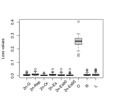
(a) $(300,75,0)$

(b) $(300,75,10^{-6})$

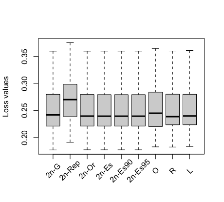
(c) $(300,75,10)$

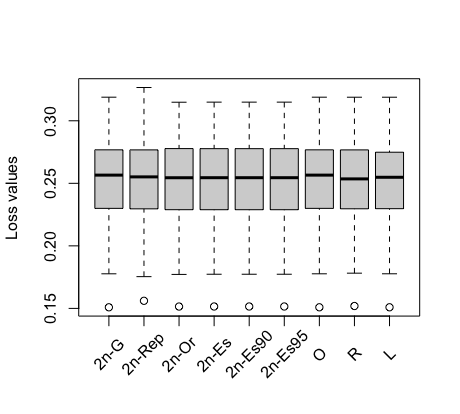
(d) $(300,75,10^{1.5})$

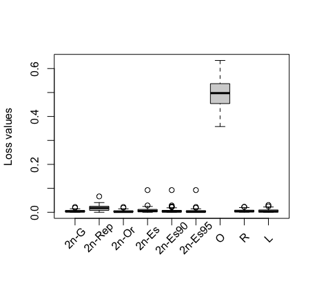
(e) $(300,150,0)$

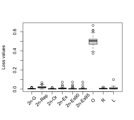
(f) $(300,150,10^{-6})$

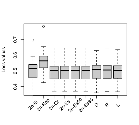
(g) $(300,150,10)$

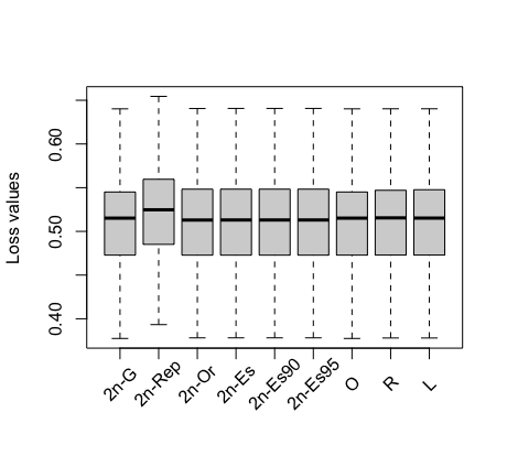
(h) $(300,150,10^{1.5})$

Figure 5: Additional displays to Figure 1, and 2. Boxplots of the observed same-X loss values from the 50 replications. Each plot is labeled with the $(n,p,\tau)$ value used.

A.7 Codes

A.7.1 Codes for mtp data cleaning

  hh2<-topo
  hh2<-na.omit(hh2)
  index<-c()
  for(i in 1:ncol(hh2)){
    if (length(unique(hh2[,i]))<30) index<-append(index,i)
  }
  set.seed(40000)
  cut_ind<-sample(nrow(hh2),size = 180,replace = FALSE)
  hh2<-hh2[cut_ind,]
  hh2<-sapply(hh2,as.numeric)
  #removing zero-valued columns
  hhx<-hh2[,-c(index,216,217,218,221,222,223,225:261,267)];hhy<-hh2[,267]
  hhx<-cbind(1,hhx)