Probing the two-body decaying dark matter scenario with weak lensing and the cosmic microwave background.
Decaying dark matter (DDM) scenarios have recently re-gained attention due to their potential ability to resolve the well-known clustering (or ) tension between weak lensing (WL) and cosmic microwave background (CMB) measurements. In this paper, we investigate a well-established model, where the original dark matter (DM) particle decays into a massless and a massive daughter particles. The latter obtains a velocity kick during the decay process resulting in a suppression of the matter power spectrum at scales that are observable with WL shear observations. We perform the first fully nonlinear WL analysis of this two-body decaying dark matter (DDM) scenario including intrinsic alignment and baryonic feedback processes. We thereby use the cosmic shear band power spectra from the KiDS-1000 data combining it with temperature and polarization data from Planck to constrain the DDM model. We report new limits on the decay rate and mass splitting parameters that are significantly stronger than previous results, especially for the case of low mass splittings. Regarding the tension, we find a reduction from about 3 to 2 depending on which statistical measure is applied. We therefore conclude that the two-body DDM model is able to reduce the tension without convincingly solving it. Our emulator to model the nonlinear DDM power spectrum is published as part of the publicly available code DMemu at https://github.com/jbucko/DMemu.
Key Words.:
dark matter, cosmological parameters, large-scale structure of Universe1 Introduction
The standard -cold dark matter (CDM) cosmology provides an outstanding description of the Universe explaining a wide range of cosmic observations, such as the cosmic microwave background (CMB), baryonic acoustic oscillations (BAO), large-scale structure formation or Big Bang nucleosynthesis (BBN). Despite its tremendous success, there are still questions as to which CDM, as understood nowadays, cannot provide satisfying answers, including the nature of dark matter (DM) and dark energy. Moreover, with progressively precise measurements, several discrepancies within the model have emerged. An example of such a discrepancy is the mild yet persistent clustering amplitude tension between CMB and weak lensing (WL) measurements, often expressed via the parameter , with and describing the clustering amplitude and the total matter abundance. More specifically, CMB measurements from Planck collaboration yield (Planck Collaboration et al., 2020a) while a variety of low-redshift surveys report consistently lower values. For example, the Kilo-Degree Survey (KiDS, Kuijken et al., 2019; Giblin et al., 2021; Hildebrandt, H. et al., 2021) obtains a value of (Asgari et al., 2021) in agreement with (albeit slightly lower than) results from the Hyper Supreme-Cam (HSC, Aihara et al., 2017; Hamana et al., 2020) and the Dark Energy Survey (DES, The Dark Energy Survey Collaboration, 2005; Amon et al., 2022).
It remains unclear whether the tension emerges from an insufficient modelling of the nonlinear clustering of matter (e.g. Tan et al., 2023; Aricò et al., 2023), the modelling of cosmic shear (García-García et al., 2021) or one has to look beyond standard CDM. Resolving the tension can be achieved by suppressing the matter power spectrum at scales - h/Mpc, which most substantially influence the clustering amplitude value (e.g. Amon & Efstathiou, 2022). Such suppression may be obtained by a number of extensions of CDM, such as cold-warm dark matter (Schneider et al., 2020a; Parimbelli et al., 2021), cannibal dark matter (Pappadopulo et al., 2016), models involving interactions between dark matter and dark radiation at early times (Cyr-Racine et al., 2016; Vogelsberger et al., 2016; Rubira et al., 2023), scenarios introducing an interaction between dark matter and dark energy (Pourtsidou et al., 2013; Poulin et al., 2022, and references therien), baryons and dark energy (Ferlito et al., 2022) or models assuming unstable dark matter particles (Enqvist et al., 2015, 2020; Murgia et al., 2017; Abellán et al., 2021; Chen et al., 2021; Bucko et al., 2023).
The class of decaying dark matter models includes several different scenarios. In the simplest case, a fraction of dark matter decays into a relativistic component (often assumed to be dark radiation). However, such a model is strongly constrained by CMB observations (see e.g. Hubert et al., 2021; Simon et al., 2022; Bucko et al., 2023) as it affects the cosmic background evolution. An alternative and only somewhat more complex scenario assume the initial dark matter particles decay into a pair of massless and massive particles, the latter obtaining a velocity kick during the decay process. This scenario is referred to as a two-body decaying dark matter model and will be denoted as DDM hereafter.
A direct consequence of the DDM model is the free streaming process of the stable decay products which alters the gravitational collapse of cosmic structures. This effect is relevant at scales set by the free-streaming length of the stable daughter particles, thus by the magnitude of the velocity kicks () they receive as a consequence of energy-momentum conservation. As a result, the matter power spectrum gets suppressed during late times at scales above h/Mpc Wang & Zentner (2012).
In addition to the aforementioned reason, there are arguments motivated by particle physics to consider models in which dark matter is not stable over cosmic time. First of all, such a stability condition does not emerge naturally, i.e. usually requires additional assumptions such as symmetry (Hambye, 2011). Moreover, there are numerous theoretical models involving dark matter decays, such as sterile neutrinos (Abazajian et al., 2012; Adhikari et al., 2017), R-parity violation (Berezinsky et al., 1991; Kim & Kim, 2002) or super Weakly Interacting Massive particles (Covi et al., 1999; Feng et al., 2003).
The two-body decaying dark matter model (DDM) has been studied from various angles over the last decade, e.g. by using perturbation theory (Wang & Zentner, 2012; Abellán et al., 2021; Simon et al., 2022) or -body simulations ranging from individual galaxies (Peter & Benson, 2010) to the large-scale structure (Cheng et al., 2015). For example, Mau et al. (2022) obtained constraints on the DDM model based on Milky Way satellite counts while Wang et al. (2013) and Fuß & Garny (2022) used Lyman- forest data to constrain the two-body decay rate in the regime of low-mass splittings. Additionally, Abellán et al. (2021) and Simon et al. (2022) considered Planck CMB observations together with supernova type Ia (SNIa) data and BAO to derive constraints on two-body decays. After including priors from WL observations, they report a reduction of the -tension for a best-fitting DDM model with Gyr and % (Simon et al., 2022).
In this work, we perform the first WL analysis of the DDM model using cosmic shear data from the KiDS-1000 survey (Asgari et al., 2021). The nonlinear clustering predictions are thereby modelled using an emulator based on a suite of -body simulations. Next to the WL analysis, we also perform a reanalysis of the Planck 2018 CMB temperature and polarisation data as well as a combined WL plus CMB modelling investigating, in particular, the potential of DDM to solve the clustering tension.
Our paper is organized as follows; in Section 2, we describe basic physics and implications of DDM model, while Section 3 provides a detailed overview of our modelling of WL and CMB observables. In Section 4, we comment on choices made in relation to model inference and in Section 5, we describe our results and compare them to recent studies before concluding in Section 6. In Appendix A, we compare the results of our -body simulations to previous studies. Appendix B discusses the cosmology dependence of the DDM effects and Appendix C studies the effects two-body decays and baryons have on WL and CMB observables. In Appendix D, we study more closely the tension between WL and CMB data in the context of the DDM model and, finally, Appendix E provides more detailed information about parameters we obtain from model inference.
2 Two-body decaying Dark Matter
In the two-body decaying dark matter (DM) model (DDM model), an original (mother) DM particle decays into a slightly lighter, stable particle and a relativistic massless relic, while the energy released during the decay process is split between the two product species. We describe the basic theoretical properties of the DDM model in Section 2.1, in Section 2.2 we discuss our DDM -body simulations and, finally, we introduce a new emulator of the DDM nonlinear matter power spectra in Section 2.3.

2.1 Theory
The DDM model is simple enough to be described by two phenomenological parameters. The first parameter is the decay rate controlling the frequency of the decay processes. The second parameter corresponds to the velocity kick of the massive daughter particle which is directly linked to the mass ratio between the mother and daughter particles. Some authors replace the velocity kick magnitude with the ratio of the rest-mass energy
| (1) |
where and denote the rest mass of the warm daughter and decaying cold mother DM particles, respectively (see e.g. Blackadder & Koushiappas, 2014). The momentum of the daughter particle in the centre-of-momentum frame is (Abellán et al., 2021) where is the speed of light. Note that in the non-relativistic limit, we obtain a simple relation .
The background evolution of the energy densities of both the cold (mother) and warm (daughter) DM species as well as the mass-less, dark-radiation (daughter) component can be written as (Wang & Zentner, 2012)
| (2) | |||
| (3) | |||
| (4) |
or using instead of particle masses
| (5) | |||
| (6) | |||
| (7) |
In the above equations, is the conformal Hubble parameter and the energy density of species ‘’. The subscripts ‘dcdm’, ‘wdm’ and ‘dr’ refer to the cold, warm, and massless species. Dots denote derivatives with respect to physical time and stands for the scale factor.
Next to the two model parameters and , we include a third parameter
| (8) |
which allows for a scenario where only a faction of the total, initial DM fluid is unstable (while the remaining DM corresponds to a stable CDM particle). Here we have introduced the abundances of the stable () and unstable () dark matter species, respectively. With the above description, one can in principle study the full parameters space of two-body decays taking arbitrary , and values, with limiting cases , or approaching CDM cosmology and approaching one-body decays. However, as recent studies have demonstrated (Wang & Zentner, 2012; Mau et al., 2022, and references therein), the DDM models with very large decay rate and velocity kicks are ruled out by observations as they lead to a strong power suppression at h/Mpc. We, therefore, focus on the regime with late-time decays () and non-relativistic velocity kicks () throughout this paper.
2.2 Simulations
Considering only non-relativistic decays, we implement the DDM model into the -body code PKDGRAV3 (Potter et al., 2017), a tree-based gravity solver based on fast multi-pole expansion and adaptive time-stepping. Following the theoretical description (5)-(7), we find that at first order, the background equations remain unmodified. With this approximation, there is no energy transfer between the radiation and dark matter components caused by the decay process. Therefore, we keep the background cosmology implementation of PKDGRAV3 unchanged and implement only the non-relativistic velocity kicks received by the WDM particles. Note that this differs from the one-body DDM model studied in Bucko et al. (2023) where the background evolution had to be modified.
The two-body decays are implemented into PKDGRAV3 via a function pkdDecayMass, which is revisited at each global integration time step (separated by a time interval ). The decay probability of a given (not yet decayed) particle at time step is . Thus, a number of simulation particles undergo the decay process, where denotes the number of unstable DCDM particles at time step . The particles that are about to decay are chosen randomly from all CDM particles. Immediately after the decay they obtain a uniform velocity kick in a random direction. Importantly, these particles are flagged and added into a set of already decayed particles in order to be excluded from the decay process occurring in future time steps.
In Fig. 1, we plot the ratios of simulated DDM to CDM power spectra for varying values of , , and (see panel a, b, and c). In general, the two-body decaying DM model leads to a suppression of the total matter power spectrum at small scales leaving the large scales unchanged. The amplitude of the suppression, as well as the scale of the downturn, depend on the values of the DDM parameters. The fraction of decaying DM as well as the decay rate both affect the amplitude of the suppression while the value of the velocity kick primarily influences the position of the downturn along the -axis. The latter can be understood by the fact that larger streaming velocities are able to affect the formation of structures at larger scales.
The redshift dependence of the power suppression is shown in panel (d) of Fig. 1. Not surprisingly, the amplitude of the suppression increases towards lower redshifts. This behaviour is caused by the fact that more particles decay with time causing a reduction of the clustering process compared to CDM.
We run a suite of -body simulations for decay rates Gyr-1 and velocity kicks . All our simulations are run assuming a fiducial cosmology with parameters and . We obtain converged results at the scales h/Mpc for box sizes of Mpc/h and particle numbers of (depending of a specific DDM configuration). We compared the output of our simulations to results from previous works and find a good level of agreement (see Appendix A). As we are primarily interested in the ratio of the nonlinear power spectra between the DDM and CDM models, the cosmology dependence is factored out to a large extent; we test that the impact of the cosmology is much smaller than the suppression due to the two-body decays.
2.3 Emulating the impact of dark matter decays
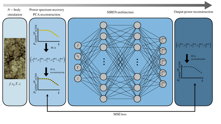
In order to carry out a Bayesian inference analysis (Section 4), we need a fast modelling framework to explore the vast parameter space of astrophysics, cosmology, and dark matter models. As -body simulations are not fast enough for this purpose, we build an emulator to account for the different DDM parameters. The basic characteristics of our emulator-building procedure are shown in the flowchart of Fig. 2. First, we run 100 gravity-only simulations for different dark matter parameters (, , and ) and measure the nonlinear matter power spectra up to /Mpc between and . In the next step, we perform a principal component analysis (PCA, see e.g. Aurélien, 2019) on the ratios of DDM and CDM matter power spectra . We find that five PCA components are sufficient to describe the ratio of spectra with a reconstruction error of %.
Next, we train a neural network to model these five PCA components of the simulated power spectra ratios for a given parameter vector (). The network output is then transformed back from the PCA representation to the power spectra ratios before being compared to the original (simulated) ratios used for the training and testing of the emulator. During the network training process, we minimise the differences between the predicted and true power spectra ratios in the training set. We consider the mean squared error (MSE) metric to quantify the differences.
We choose the sinusoidal representation networks (SIRENs; Sitzmann et al. 2020) architecture for building our DDM emulator. SIRENs have been successfully shown to have good interpolation and signal reconstruction properties (Sitzmann et al., 2020). The main difference compared to standard feed-forward architectures is replacing the commonly assumed ReLU activation function with a sine function. We use the architecture with two hidden layers each having 1024 neurons to perform the emulation task. During the training, we optimize the MSE with the Adam optimizer (Kingma & Ba, 2014). To further fine-tune the SIREN architecture, we perform a hyperparameter optimization for the network’s learning rate and regularization strength using the Bayesian Optimization and Hyperband (BOHB) method (Falkner et al., 2018). The entire training is performed using the PyTorch (Paszke et al., 2019) machine learning framework.
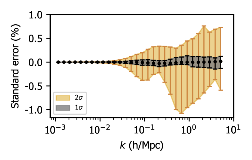
After training we test the emulator on separate data (i.e. the test set) and monitor the prediction mismatch in each of the 30 -bins. We show the emulation performance in Fig. 3 and demonstrate that both 1 and 2 errors stay below 1%. Our emulator can thus efficiently predict the response of decays on the nonlinear matter power spectrum . The prediction time of our emulator is a few milliseconds. With this tool, we can model the nonlinear power spectrum in the presence of dark matter decays as
| (9) |
where is obtained by multiplying the nonlinear power spectrum from the revised_halofit method (Takahashi et al., 2012).
3 Data sets and modelling framework
Here we first describe the observational data that we use to study the DDM model. Later, in Section 3.2 and 3.3, we present our modelling framework.
3.1 Data sets
Galaxy WL is a particularly promising observable to probe decaying dark matter models as such scenarios tend to affect structure formation at late times and small cosmological scales. However, while primarily focusing on the WL analysis, we also include CMB data into our analysis. Although the CMB radiation is not sensitive to the DDM model parameters, it helps constrain the cosmological parameters and provides insights into the issue of the -tension.
In our study, we use the following observational data sets:
-
The WL cosmic shear data of the KiDS-1000 data release, obtained in five redshift bins between (Asgari et al., 2021). We use the band power angular spectra measured at scales , and
-
The Planck 2018 high- power spectra () of temperature (TT), polarization (EE) and their cross (TE) obtained from Planck Collaboration et al. (2020b).
In the following subsections, we will discuss how we predict these observations in our modelling framework.
3.2 Cosmic Shear modelling for KiDS-1000
The KiDS-1000 catalogue provides information about the shear of over 20 million galaxies divided into five tomographic bins between and . The catalogue provides the basis of the auto and cross-correlation band power of all five redshift bins. With eight data points for each spectrum, the KiDS-1000 band power contains a total of 120 observational data points with correlated errors from the corresponding covariance matrix.
3.2.1 Nonlinear matter power spectrum
We use the public version of the Boltzmann Solver CLASS (Blas et al., 2011) to calculate the matter power spectrum for any given set of cosmological parameters. For the nonlinear modelling, we rely on the revised halofit method (Takahashi et al., 2012) implemented in CLASS. Following Planck Collaboration et al. (2020a), we assume a single massive neutrino species with fixed mass eV throughout this work.
The process of baryonic feedback causes gas to be expelled out of galaxies and clusters leading to a suppression of the matter power spectrum at small cosmological scales (e.g. van Daalen et al., 2011; Schneider & Teyssier, 2015; Chisari et al., 2019). Note that this suppression is similar in shape to the one caused by DM decays (Hubert et al., 2021) making it particularly important to include baryonic feedback in our modelling pipeline. We use BCemu111The BCemu code can be found at https://github.com/sambit-giri/BCemu. (Giri & Schneider, 2021), an emulation tool providing the suppression due to baryonic feedback described in Schneider et al. (2019). is a function of seven baryonic parameters and one cosmological parameter, namely the ratio of the baryonic and total matter abundance. However, we use the reduced three-parameter model presented in Giri & Schneider (2021) where four parameters are fixed based on results from hydrodynamical simulations. The three-parameter model consists of two parameters describing the gas distribution (log, ) and one parameter describing the stellar mass () around galaxies and clusters. We refer to Giri & Schneider (2021) for the detailed description of the model.
Finally, the response function from the two-body DM decays is multiplied with the nonlinear, baryonified power spectrum as shown in Eq. 9. It is obtained from the emulator described in Section 2.3. This modular method assumes that all dependence on cosmological parameters is captured by the power spectrum from the revised halofit. At the same time, the responses from the baryonification and the two-body decays remain independent of cosmology. Regarding the baryonification method, this assumption has been validated before (Schneider et al., 2020a, b). In Appendix B, we validated this assumption for the DDM model.
3.2.2 Intrinsic alignment
The effects from intrinsic galaxy alignments are modelled assuming the nonlinear alignment model (NLA) as described in Hildebrandt et al. (2016) and first published in Hirata & Seljak (2004). Intrinsic alignment enters the band powers modelling via window function (see eq. 9 in Bucko et al., 2023) that goes into galaxy-intrinsic and intrinsic-intrinsic terms of cosmic shear angular power spectrum. Among the two intrinsic alignment parameters and , we fixed the latter one to zero, following the approach used in the standard KiDS-1000 analyses (Asgari et al., 2021).
3.2.3 Angular power spectrum
We investigate the impact of decaying dark matter on structure formation through the analysis of the cosmic shear angular power spectrum, including both auto-correlation and cross-correlation power spectra between different galaxy populations (tomographic bins). Our modelling approach follows the methodology presented in Bucko et al. (2023), and we refer the reader to that work for a more comprehensive description.
We use the multi-purpose cosmology calculation tool PyCosmo (Tarsitano et al., 2020) to model the cosmic shear angular power spectrum. The angular power is then converted into band powers following Joachimi et al. (2021). In Fig. 10, we show all band power coefficients together with the respective error bars. The auto- and cross-band powers measurements are illustrated in five redshift bins between to .
3.3 CMB modelling
The Boltzmann Solver CLASS can also be used for theoretical modelling of the CMB temperature and polarization data. Since the work of Abellán et al. (2021), CLASS comes with an implementation of the DDM model which we use throughout this work222https://github.com/PoulinV/class_decays. To investigate the effects of DDM cosmology on CMB data, we model temperature and polarization power spectra from the Planck 2018 data release (Planck Collaboration et al., 2020b). We adopt the same methodology as the one introduced in Bucko et al. (2023) and refer the reader to this work for more details. Note, however, that our pipeline is tested for the CDM cosmology reaching an excellent agreement with the results from Planck Collaboration et al. (2020a). A comparison can be found in appendix A of Bucko et al. (2023).
4 Model inference
We perform a number of Markov Chain Monte Carlo (MCMC) samplings in order to infer the posterior probability distribution of cosmological, baryonic, intrinsic alignment and two-body DDM parameters based on the WL data from KiDS and the CMB observations from Planck. We employ the Strech Move ensemble method implemented within emcee package (Foreman-Mackey et al., 2013) to sample from the posterior distribution.
An overview of the sampled parameters and the prior choices are listed in Tab. 1. We use flat priors for all cosmological parameters except for the optical depth where we assume a Gaussian prior , as explained in Section 3.1 of Bucko et al. (2023). For the DM abundance () and the amplitude of the primordial power spectrum (), we use priors that are wide enough to comfortably include the WL posteriors found by Asgari et al. (2021). Note that represents the initial DM abundance and, as we assume only late-time decays, this parameter describes the total initial DM budget in both CDM and DDM scenarios. For the baryon abundance , Hubble constant and spectral index , which cannot be well constrained by WL alone, we choose the prior that is as wide as possible to span the values found by surveys (e.g. CMB data) that are more sensitive to these parameters. The prior range for the intrinsic alignment parameter is wide enough to include the posterior distribution of this parameter found by Asgari et al. (2021). The Planck absolute calibration was probed under Gaussian prior 333https://wiki.cosmos.esa.int/planck-legacy-archive/index.php/CMB_spectrum_%26_Likelihood_Code. We further impose flat priors on the baryonic parameters and covering the full range of the BCemu parameters. For the DDM decay rate () and the velocity kick magnitude (), we assume flat priors for both and spanning from CDM values up to the upper boundary limited by the range of the DDM emulator (see Tab. 1).
| Parameter name | Acronym | prior | range |
| (Initial) DM abundacne | flat | [0.051, 0.255] | |
| Baryon abundance | flat | [0.019, 0.026] | |
| Scalar amplitude | flat | [1.0, 5.0] | |
| Hubble constant | flat | [0.6, 0.8] | |
| Spectral index | flat | [0.9, 1.03] | |
| Optical depth | normal | ||
| Intrinsic alignment amplitude | flat | [0.0, 2.0] | |
| Planck calibration parameter | normal | ||
| First gas parameter (BCemu) | flat | [11.0, 15.0] | |
| Second gas parameter (BCemu) | flat | [2.0, 8.0] | |
| Stellar parameter (BCemu) | flat | [0.05, 0.40] | |
| Decay rate (Gyr-1) | flat | [, ] | |
| Velocity kick magnitude (km/s) | flat | [0.00, 3.69] |
In both the WL and CMB setups, we assume Gaussian likelihoods. In the case of the CMB, we use a marginalized, light-weight version of the full Planck likelihood called Plik_lite (Prince & Dunkley, 2019; Planck Collaboration et al., 2020b), being an affordable approximation in case of DDM. Abellán et al. (2021) demonstrates that using Plik_lite for DDM produces only a negligible difference on recovered posteriors compared to a full Planck analysis. Plik_lite also comes with the marginalized version of the covariance matrix, which we use throughout this work. In the case of WL, we use the band powers covariance matrix as published in Asgari et al. (2021). To assess the convergence of our chains, we apply the Gelman-Rubin criterion (Gelman & Rubin, 1992) assuming the chains to be converged at .
We use two different metrics to assess the tension between CMB and WL observations within the assumed cosmological model. The first one is the standard Gaussian metric (see e.g. Asgari et al., 2021), which is defined as
| (10) |
where stands for the variance of the measurements from the two data sets. Note that the Gaussian metric assumes a Gaussian posterior distribution of the parameter of interest and, importantly, is agnostic about how well the underlying data are being fitted. Due to these short-comings, we also employ the Difference in maximum a posteriori criterion (Raveri & Hu, 2019). This metric is defined as
| (11) |
where , , and correspond to the minimum chi-squared values from the WL, the CMB, and the combined analysis. The criterion evaluates the incapability of a combined analysis to approach the goodness of fit of the individual analyses, i.e. when either of the data sets is fitted separately. In terms of , the tension is quantified as .
Although the emulator presented Section 2.3 accounts for the three parameters , and , we fix the fraction of decaying to stable DM to unity (). This means that we restrict our analysis to the case of a universe with one initial (unstable) DM fluid leaving the further investigation of a multi-fluid DM sector to future work.
5 Results
In the first part of this section, we describe the constraints on two-body decays from WL and CMB observations and report our findings regarding baryonic physics. In the second part, we revisit the impact of the DDM model on the tension before concluding with a discussion about how well the observational data can be fitted within the DDM model.
5.1 Derived constraints on two-body decays
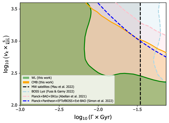
We obtain the constraints on the decay rate and velocity kick magnitude by marginalizing over cosmology, baryons and nuisance parameters. We display the outcome in Fig. 4, showing the DDM posteriors at the 95% credible intervals as obtained from WL (green) and CMB (orange) analysis. In both cases, the obtained constraints are in agreement with CDM showing no hint of decay in the DM sector. Fig. 4 also includes a comparison of our findings with several recent studies: Mau et al. (2022) (black) focusing on Milky Way satellites, Fuß & Garny (2022) (light blue) examining the impact on Lyman- forest, and Abellán et al. (2021) and Simon et al. (2022) (pink and blue, respectively) using Planck 2018, SNIa, and BAO data. We note that our CMB posteriors are consistent with previous CMB studies, in particular with the results of Simon et al. (2022). Our limits are slightly stronger than those of Abellán et al. (2021) while exhibiting similar hyperbolic contour trends. Milky way satellites as probed by the DES collaboration (Mau et al., 2022) are sensitive to decay rate and rule out half-life times Gyr, while Lyman- showing to be less sensitive to two-body decays than MW satellites. Finally, the WL data alone provides the most stringent constraints, excluding regions where the following conditions hold at 95% credible intervals:
| (12) | |||
| (13) |
Hence, within the parameter space of DDM and the data sets analysed in this study, WL data impose much stronger limits compared to CMB observations444It is important to note that in our analysis we do not include the CMB lensing effect.. This is mainly due to the fact that, unlike for the case of 1-body decays (Bucko et al., 2023), the two-body DDM model does not significantly affect the background evolution of the Universe leaving the signal from the late-time integrated Sachs-Wolfe effect unchanged. More discussions about the effects of two-body decays on the CMB signal can be found in Appendix C.
5.2 Revisiting the tension between WL and the CMB
As a next step, we investigate to what extent the DDM model is able to alleviate the tension between lensing and CMB data. In contrast to previous findings (e.g. Abellán et al., 2021, 2022; Tanimura et al., 2023), we thereby argue that the DDM model is unable to significantly reduce the systematic shift between the clustering signal predicted from the CMB and the KiDS-1000 WL survey.
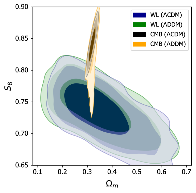
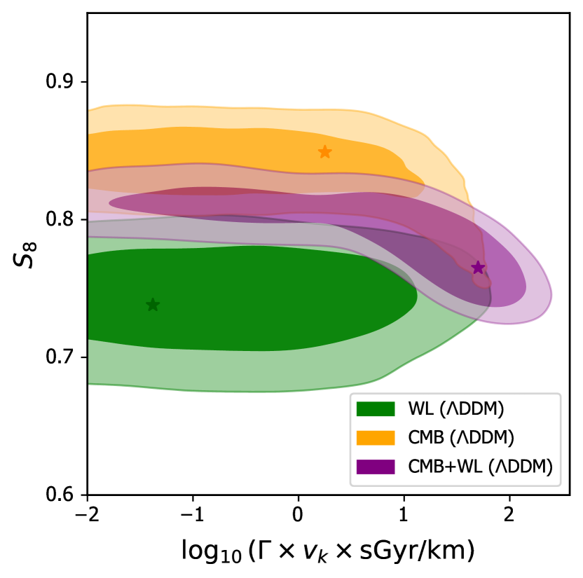
In Fig. 5 we illustrate the posterior contours as obtained from the individual WL and CMB data analyses for both the CDM (dark blue and black) and the DDM model (green and orange). We observe only a marginal change of the WL and CMB contours when going from CDM to DDM case both at the 68% and 95% confidence level. However, at the 99% confidence level the CMB contours reveal a prominent feature pointing towards low -values in apparent agreement with the WL analysis.
Applying the criterion defined in Eq. (11), we obtain a mutual tension of between WL and CMB data for the case of CDM. Including two-body decays, the tension is reduced to . Using the Gaussian metric defined in Eq. (10), we obtain a -tension of for CDM and for DDM. The difference between the two measures confirms the non-Gaussian shape of the CMB posteriors.
The origin of the non-Gaussian tail in the plane (visible in Fig. 5) can be better understood by looking at Fig. 6, in which we plot the posterior distribution of against the product of DDM parameters (). We can see that for large values of , the posterior obtained from the CMB analysis bends downwards preferring smaller values of . However, this downturn happens at a part of parameter space that is not favoured by the WL analysis. Instead of fully overlapping with the WL posteriors (green), the CMB contours (orange) rather wrap around them only leading to a slight overlap of the 95 percent confidence regions.
Based on the analysis above, we conclude that although the two-body decaying dark matter model (DDM) alleviates the tension to some degree, it does not provide a convincing solution to it. Furthermore, the model does not yield improved fits to either the individual CMB or WL data (see Tab. 2) despite the two additional model parameters and . For further tests of the DDM model we refer to Appendix D.
Fitting the combined WL+CMB data, we obtain a preference for a model with non-zero DDM parameters. The best fitting values are and , compatible with the overlap region of CMB and WL posteriors. See Appendix E for the full results from our MCMC analyses. These findings align with the conclusions of Simon et al. (2022) who added a Gaussian prior with the value from KiDS to their CMB analysis. However, given the original tension between WL and CMB data, it is not surprising to obtain a preference for non-vanishing DDM parameters in the combined data analysis. We want to stress that this is by no means a signal of a departure from CDM but rather a natural consequence of the internal tension between the two data sets. This interpretation is confirmed by the fact that the posteriors form the individual analysis shown in Fig. 5 do neither show significant overlap in the CDM nor in the DDM case.
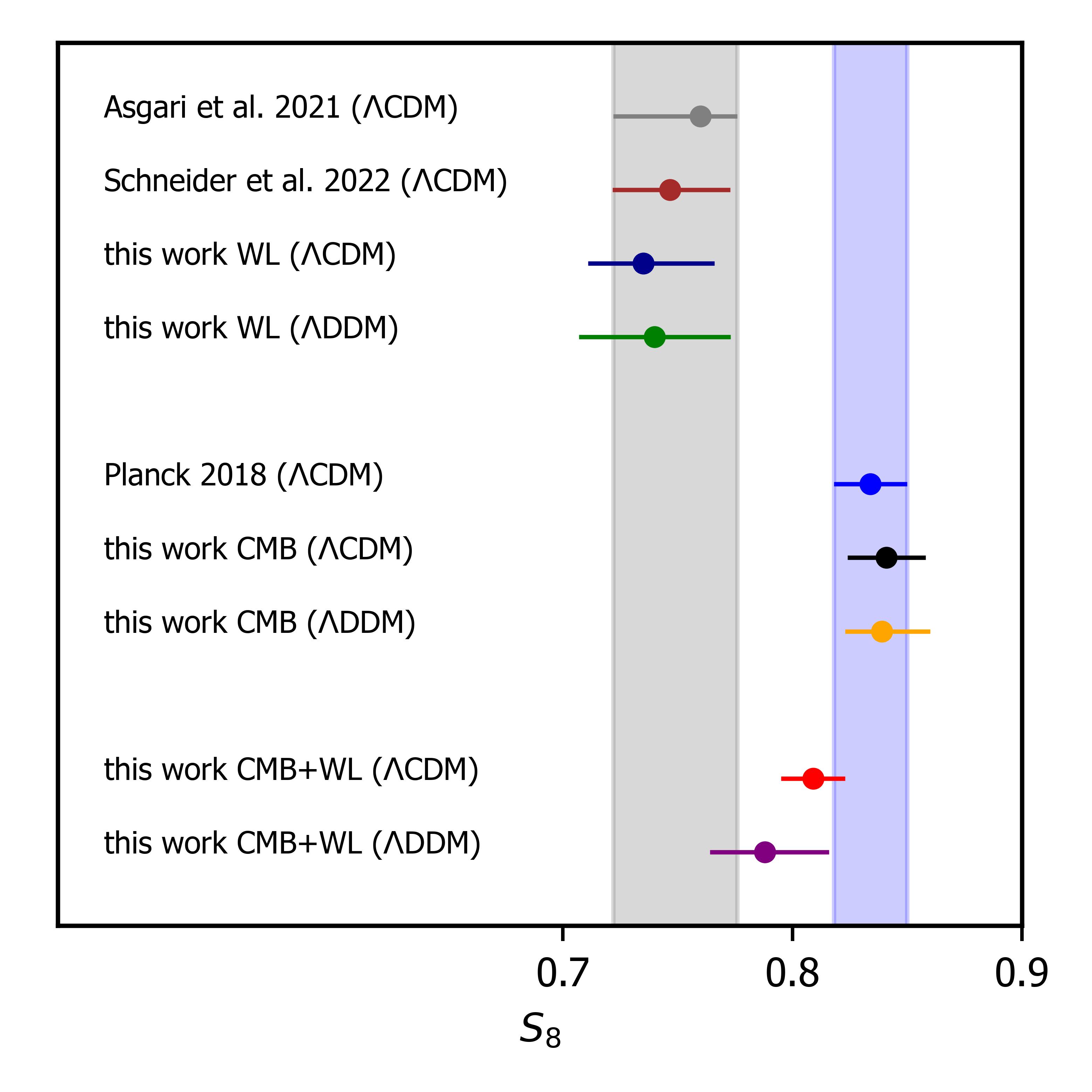
The constraints inferred for all sampled parameters in our MCMC runs in case of CMB-only, WL-only and combined analysis can be found in Tab. 3 and Tab. 4 of Appendix E. In particular, the values of from our CMB and WL analyses are compared to the results of Asgari et al. (2021), Schneider et al. (2022) and Planck Collaboration et al. (2020a) in Fig. 7. Details about tests of our MCMC pipeline and the related discussion can be found in Appendix A of Bucko et al. (2023).
6 Summary & conclusion
A dark matter (DM) scenario including particle decay forms a natural extension to the minimal model of a cold, stable, and collisionless DM particle. In this work, we investigate the case of two-body DM decays where particles decay into a massless and a massive daughter particle, the latter obtaining a velocity kick as a result of the decay process. This model has been studied in different contexts in the past (e.g. Peter et al., 2010; Wang & Zentner, 2012; Cheng et al., 2015; Fuß & Garny, 2022) and has been proposed as a potential solution to the tension (Abellán et al., 2021, 2022; Simon et al., 2022).
In this paper, we perform the first fully nonlinear analysis of WL and CMB data for the two-body decaying dark matter (DDM) scenario. Based on a suite of -body simulations, we construct a neural network-based emulator to obtain fast predictions of nonlinear matter power spectra for arbitrary values of the decay rate (), the decay-induced velocity kick () and the fraction of decaying to total DM (). We then include the emulator into our pipeline predicting WL observations and perform an MCMC analysis with WL data from KiDS-1000 and CMB data from Planck 2018.
We present improved constraints on the two-body decaying DM parameters based on the WL data from KiDS-1000. Our constraints are significantly stronger compared to previous results. Specifically, we exclude models with Gyr and km/s. Fig. 4 provides a summary of our constraints from the WL and the CMB, along with previous results from the literature.
When considering the clustering (or ) tension between KiDS-1000 and Planck 2018, we observe a marginal improvement of 0.3 with DDM compared to the original 3.0 tension measured in the CDM model. We, therefore, conclude that the two-body DDM scenario is unable to convincingly resolve the clustering tension between WL and CMB observations. Note that previous work obtaining different conclusions (e.g. Abellán et al., 2021, 2022; Simon et al., 2022; Tanimura et al., 2023) did not include a full, self-consistent modelling of the WL signal and were therefore unable to directly test the tension in the case of DDM.
A further step forward with respect to the current analysis could involve the analysis of the DDM model using Dark Energy Survey (DES) observations along with the possible addition of galaxy clustering and galaxy-galaxy lensing. Furthermore, including additional low-redshift data sets, such as eBOSS and SNIa, could lead to stronger constraints on parameters such as and allowing for a more precise determination of the DM parameters. Finally, we expect data from Euclid and the Vera C. Rubin Observatory to significantly improve current limits on DM decays.
The emulator of two-body decays developed in this study is now publicly available as the DMemu Python package. We welcome researchers to incorporate this package into their data analysis pipelines and further test the DDM model.
Acknowledgements.
We thank Douglas Potter and Jonathan Hubert for helpful discussions and technical support. This work is supported by the Swiss National Science Foundation under grant number PCEFP2_181157. Nordita is supported in part by NordForsk.References
- Abazajian et al. (2012) Abazajian, K. N., Acero, M. A., Agarwalla, S. K., et al. 2012, Light Sterile Neutrinos: A White Paper
- Abellán et al. (2021) Abellán, G. F., Murgia, R., & Poulin, V. 2021, Phys. Rev. D, 104, 123533
- Abellán et al. (2022) Abellán, G. F., Murgia, R., Poulin, V., & Lavalle, J. 2022, Phys. Rev. D, 105, 063525
- Adhikari et al. (2017) Adhikari, R., Agostini, M., Ky, N. A., et al. 2017, Journal of Cosmology and Astroparticle Physics, 2017, 025
- Aihara et al. (2017) Aihara, H., Arimoto, N., Armstrong, R., et al. 2017, Publications of the Astronomical Society of Japan, 70, s4
- Amon & Efstathiou (2022) Amon, A. & Efstathiou, G. 2022, Monthly Notices of the Royal Astronomical Society, 516, 5355
- Amon et al. (2022) Amon, A., Gruen, D., Troxel, M. A., et al. 2022, Phys. Rev. D, 105, 023514
- Aricò et al. (2023) Aricò, G., Angulo, R. E., Zennaro, M., et al. 2023, DES Y3 cosmic shear down to small scales: constraints on cosmology and baryons
- Asgari et al. (2021) Asgari, M., Lin, C.-A., Joachimi, B., et al. 2021, A&A, 645, A104
- Aurélien (2019) Aurélien, G. 2019, Hands-on machine learning with Scikit-Learn, Keras, and TensorFlow: concepts, tools, and techniques to build intelligent systems (OReilly Media, Inc.)
- Berezinsky et al. (1991) Berezinsky, V., Masiero, A., & Valle, J. 1991, Physics Letters B, 266, 382
- Blackadder & Koushiappas (2014) Blackadder, G. & Koushiappas, S. M. 2014, Phys. Rev. D, 90, 103527
- Blas et al. (2011) Blas, D., Lesgourgues, J., & Tram, T. 2011, Journal of Cosmology and Astroparticle Physics, 2011, 034
- Bucko et al. (2023) Bucko, J., Giri, S. K., & Schneider, A. 2023, A&A, 672, A157
- Chen et al. (2021) Chen, A., Huterer, D., Lee, S., et al. 2021, Phys. Rev. D, 103, 123528
- Cheng et al. (2015) Cheng, D., Chu, M.-C., & Tang, J. 2015, Journal of Cosmology and Astroparticle Physics, 2015, 009
- Chisari et al. (2019) Chisari, N. E. et al. 2019, Open J. Astrophys. [arXiv:1905.06082]
- Covi et al. (1999) Covi, L., Kim, J. E., & Roszkowski, L. 1999, Phys. Rev. Lett., 82, 4180
- Cyr-Racine et al. (2016) Cyr-Racine, F.-Y., Sigurdson, K., Zavala, J., et al. 2016, Phys. Rev. D, 93, 123527
- Enqvist et al. (2015) Enqvist, K., Nadathur, S., Sekiguchi, T., & Takahashi, T. 2015, JCAP, 09, 067
- Enqvist et al. (2020) Enqvist, K., Nadathur, S., Sekiguchi, T., & Takahashi, T. 2020, JCAP, 04, 015
- Falkner et al. (2018) Falkner, S., Klein, A., & Hutter, F. 2018, in Proceedings of Machine Learning Research, Vol. 80, Proceedings of the 35th International Conference on Machine Learning, ed. J. Dy & A. Krause (Stockholmsmässan, Stockholm Sweden: PMLR), 1437–1446
- Feng et al. (2003) Feng, J. L., Rajaraman, A., & Takayama, F. 2003, Phys. Rev. Lett., 91, 011302
- Ferlito et al. (2022) Ferlito, F., Vagnozzi, S., Mota, D. F., & Baldi, M. 2022, Monthly Notices of the Royal Astronomical Society, 512, 1885
- Foreman-Mackey et al. (2013) Foreman-Mackey, D., Hogg, D. W., Lang, D., & Goodman, J. 2013, PASP, 125, 306
- Fuß & Garny (2022) Fuß, L. & Garny, M. 2022, arXiv e-prints, arXiv:2210.06117
- García-García et al. (2021) García-García, C., Ruiz-Zapatero, J., Alonso, D., et al. 2021, Journal of Cosmology and Astroparticle Physics, 2021, 030
- Gelman & Rubin (1992) Gelman, A. & Rubin, D. B. 1992, Statistical Science, 7, 457
- Giblin et al. (2021) Giblin, B., Heymans, C., Asgari, M., et al. 2021, A&A, 645, A105
- Giri & Schneider (2021) Giri, S. K. & Schneider, A. 2021, Journal of Cosmology and Astroparticle Physics, 2021, 046
- Hamana et al. (2020) Hamana, T., Shirasaki, M., Miyazaki, S., et al. 2020, Publications of the Astronomical Society of Japan, 72, 16
- Hambye (2011) Hambye, T. 2011, in Proceedings of Identification of Dark Matter 2010 — PoS(IDM2010), Vol. 110, 098
- Hildebrandt et al. (2016) Hildebrandt, H., Viola, M., Heymans, C., et al. 2016, Monthly Notices of the Royal Astronomical Society, 465, 1454
- Hildebrandt, H. et al. (2021) Hildebrandt, H., van den Busch, J. L., Wright, A. H., et al. 2021, A&A, 647, A124
- Hirata & Seljak (2004) Hirata, C. M. & Seljak, U. c. v. 2004, Phys. Rev. D, 70, 063526
- Hubert et al. (2021) Hubert, J., Schneider, A., Potter, D., Stadel, J., & Giri, S. K. 2021, Journal of Cosmology and Astroparticle Physics, 2021, 040
- Jeffreys (1961) Jeffreys, H. 1961, Theory of probability (Clarendon)
- Joachimi et al. (2021) Joachimi, B., Lin, C.-A., Asgari, M., et al. 2021, A&A, 646, A129
- Kim & Kim (2002) Kim, H. B. & Kim, J. E. 2002, Physics Letters B, 527, 18
- Kingma & Ba (2014) Kingma, D. P. & Ba, J. 2014, Adam: A Method for Stochastic Optimization
- Kuijken et al. (2019) Kuijken, K., Heymans, C., Dvornik, A., et al. 2019, A&A, 625, A2
- Mau et al. (2022) Mau, S., Nadler, E. O., Wechsler, R. H., et al. 2022, The Astrophysical Journal, 932, 128
- Murgia et al. (2017) Murgia, R., Merle, A., Viel, M., Totzauer, M., & Schneider, A. 2017, Journal of Cosmology and Astroparticle Physics, 2017, 046
- Pappadopulo et al. (2016) Pappadopulo, D., Ruderman, J. T., & Trevisan, G. 2016, Phys. Rev. D, 94, 035005
- Parimbelli et al. (2021) Parimbelli, G., Scelfo, G., Giri, S., et al. 2021, Journal of Cosmology and Astroparticle Physics, 2021, 044
- Paszke et al. (2019) Paszke, A., Gross, S., Massa, F., et al. 2019, in Advances in Neural Information Processing Systems 32 (Curran Associates, Inc.), 8024–8035
- Peter & Benson (2010) Peter, A. H. G. & Benson, A. J. 2010, Physical Review D, 82, 123521
- Peter et al. (2010) Peter, A. H. G., Moody, C. E., & Kamionkowski, M. 2010, Phys. Rev. D, 81, 103501
- Planck Collaboration et al. (2020a) Planck Collaboration, Aghanim, N., Akrami, Y., et al. 2020a, A&A, 641, A6
- Planck Collaboration et al. (2020b) Planck Collaboration, Aghanim, N., Akrami, Y., et al. 2020b, A&A, 641, A5
- Potter et al. (2017) Potter, D., Stadel, J., & Teyssier, R. 2017, Computational Astrophysics and Cosmology, 4
- Poulin et al. (2022) Poulin, V., Bernal, J. L., Kovetz, E., & Kamionkowski, M. 2022, The Sigma-8 Tension is a Drag
- Pourtsidou et al. (2013) Pourtsidou, A., Skordis, C., & Copeland, E. J. 2013, Phys. Rev. D, 88, 083505
- Prince & Dunkley (2019) Prince, H. & Dunkley, J. 2019, Phys. Rev. D, 100, 083502
- Raveri & Hu (2019) Raveri, M. & Hu, W. 2019, Phys. Rev. D, 99, 043506
- Rubira et al. (2023) Rubira, H., Mazoun, A., & Garny, M. 2023, Journal of Cosmology and Astroparticle Physics, 2023, 034
- Schneider et al. (2022) Schneider, A., Giri, S. K., Amodeo, S., & Refregier, A. 2022, Monthly Notices of the Royal Astronomical Society, 514, 3802
- Schneider et al. (2020a) Schneider, A., Refregier, A., Grandis, S., et al. 2020a, JCAP, 04, 020
- Schneider et al. (2020b) Schneider, A., Stoira, N., Refregier, A., et al. 2020b, JCAP, 04, 019
- Schneider & Teyssier (2015) Schneider, A. & Teyssier, R. 2015, JCAP, 1512, 049
- Schneider et al. (2019) Schneider, A., Teyssier, R., Stadel, J., et al. 2019, JCAP, 03, 020
- Schöneberg et al. (2022) Schöneberg, N., Abellán, G. F., Sánchez, A. P., et al. 2022, Physics Reports, 984, 1, The Olympics: A fair ranking of proposed models
- Simon et al. (2022) Simon, T., Abellán, G. F., Du, P., Poulin, V., & Tsai, Y. 2022, Constraining decaying dark matter with BOSS data and the effective field theory of large-scale structures
- Sitzmann et al. (2020) Sitzmann, V., Martel, J. N., Bergman, A. W., Lindell, D. B., & Wetzstein, G. 2020, in Proc. NeurIPS
- Takahashi et al. (2012) Takahashi, R., Sato, M., Nishimichi, T., Taruya, A., & Oguri, M. 2012, The Astrophysical Journal, 761, 152
- Tan et al. (2023) Tan, T., Zuercher, D., Fluri, J., et al. 2023, Mon. Not. Roy. Astron. Soc., 522, 3766
- Tanimura et al. (2023) Tanimura, H., Douspis, M., Aghanim, N., & Kuruvilla, J. 2023, A&A, 674, A222
- Tarsitano et al. (2020) Tarsitano, F., Schmitt, U., Refregier, A., et al. 2020, Predicting Cosmological Observables with PyCosmo
- The Dark Energy Survey Collaboration (2005) The Dark Energy Survey Collaboration. 2005, arXiv e-prints, astro
- van Daalen et al. (2011) van Daalen, M. P., Schaye, J., Booth, C. M., & Vecchia, C. D. 2011, Mon. Not. Roy. Astron. Soc., 415, 3649
- Vogelsberger et al. (2016) Vogelsberger, M., Zavala, J., Cyr-Racine, F.-Y., et al. 2016, Monthly Notices of the Royal Astronomical Society, 460, 1399
- Wang et al. (2013) Wang, M.-Y., Croft, R. A. C., Peter, A. H. G., Zentner, A. R., & Purcell, C. W. 2013, Phys. Rev. D, 88, 123515
- Wang & Zentner (2012) Wang, M.-Y. & Zentner, A. R. 2012, Phys. Rev. D, 85, 043514
Appendix A Comparing two-body decay simulations to previous work
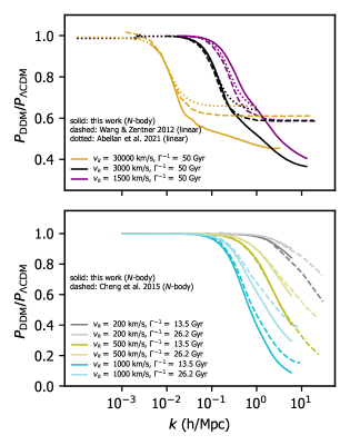
In Fig. 8, we present a comparison of our -body simulations with three other studies that have investigated the same DDM model (Wang & Zentner 2012; Cheng et al. 2015; Abellán et al. 2021). In the top panel of Fig.8, we compare linear recipes based on solving the Boltzmann hierarchy, as developed by Wang & Zentner (2012) (dashed lines) and Abellán et al. (2021) (dotted lines). The solid lines represent the results of our DDM -body simulations for . For the chosen values of and , we observe good agreement in terms of the downturn scales. However, at nonlinear scales, there are more pronounced differences between the results, which is expected due to the limitations of linear calculations at higher values of . Note that for km/s, which corresponds to 10% of the speed of light, we have concerns about the accuracy of our -body implementation. Therefore, we do not perform model inference for such extreme values of in this work.
In the bottom panel of Fig. 8, we provide a benchmark of the DDM model (for ) by comparing it with the N-body study conducted by Cheng et al. (2015) for six different sets of dark matter parameters. We find that scenarios with smaller velocity kicks ( km/s) exhibit agreement at the percent level across all scales. At the nonlinear regime ( h/Mpc) and for larger velocity kicks ( km/s), we observe larger deviations in the predicted power suppression. These deviations can be attributed to the different dark matter implementations employed by Cheng et al. (2015). However, it is important to note that scenarios with such a significant power suppression in the nonlinear regime are ruled out by observations, which favour a much weaker decrease of power at h/Mpc (Wang & Zentner 2012). Therefore, the observed differences between our results and those of Cheng et al. (2015) are not a cause for concern.
Appendix B Cosmology dependence of suppression of the matter power spectrum in DDM with respect to CDM
The effects of DDM in our study are accounted for by applying a cosmology-independent boost to the CDM nonlinear matter power spectrum, calculated using the revised_halofit method within the CLASS code. To demonstrate the validity of this approach, we conducted a test suite of -body simulations, where we kept the DDM parameters fixed at Gyr and km/s, and varied one CDM parameter at a time.
We show in Fig. 9 that this approach is a good approximation as neglecting the cosmology dependence in the applied boost results only in a second-order effect. In panels (a) to (e) of this figure, we show the impact of Hubble parameter (), clustering amplitude (), spectral index (), matter abundance () and baryon abundance (), respectively. We display the DDM boost for the fiducial cosmology of our -body simulations in solid salmon, while we plot the same quantity for the best-fit cosmology of KiDS-450 survey (Hildebrandt et al. 2016) in dashed blue. We also add a few additional models in dotted grey.
In this analysis, we find that the choice of cosmology has a noticeable impact on the DDM boost only for the parameters (panel b) and (panel d). For the remaining parameters, the choice of cosmology does not significantly affect the boost. It is important to note that the models exhibiting substantial differences assume cosmologies that are quite distinct from the fiducial one. However, even in the cases of and , the observed effects are relatively small compared to the overall amplitude of the observed boost.

Appendix C Effect of model and baryonic feedback parameters on the observables
C.1 Weak Lensing
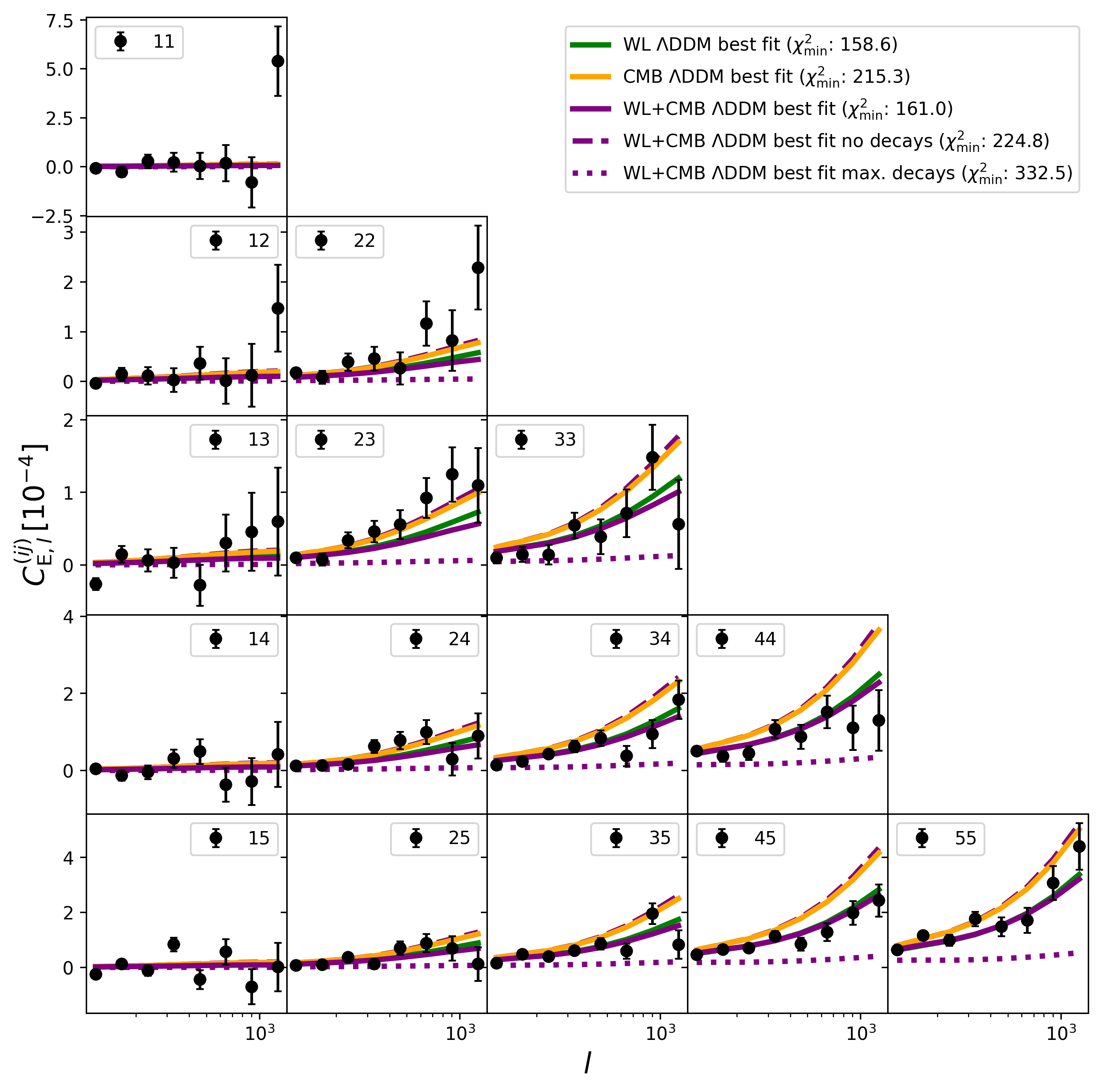
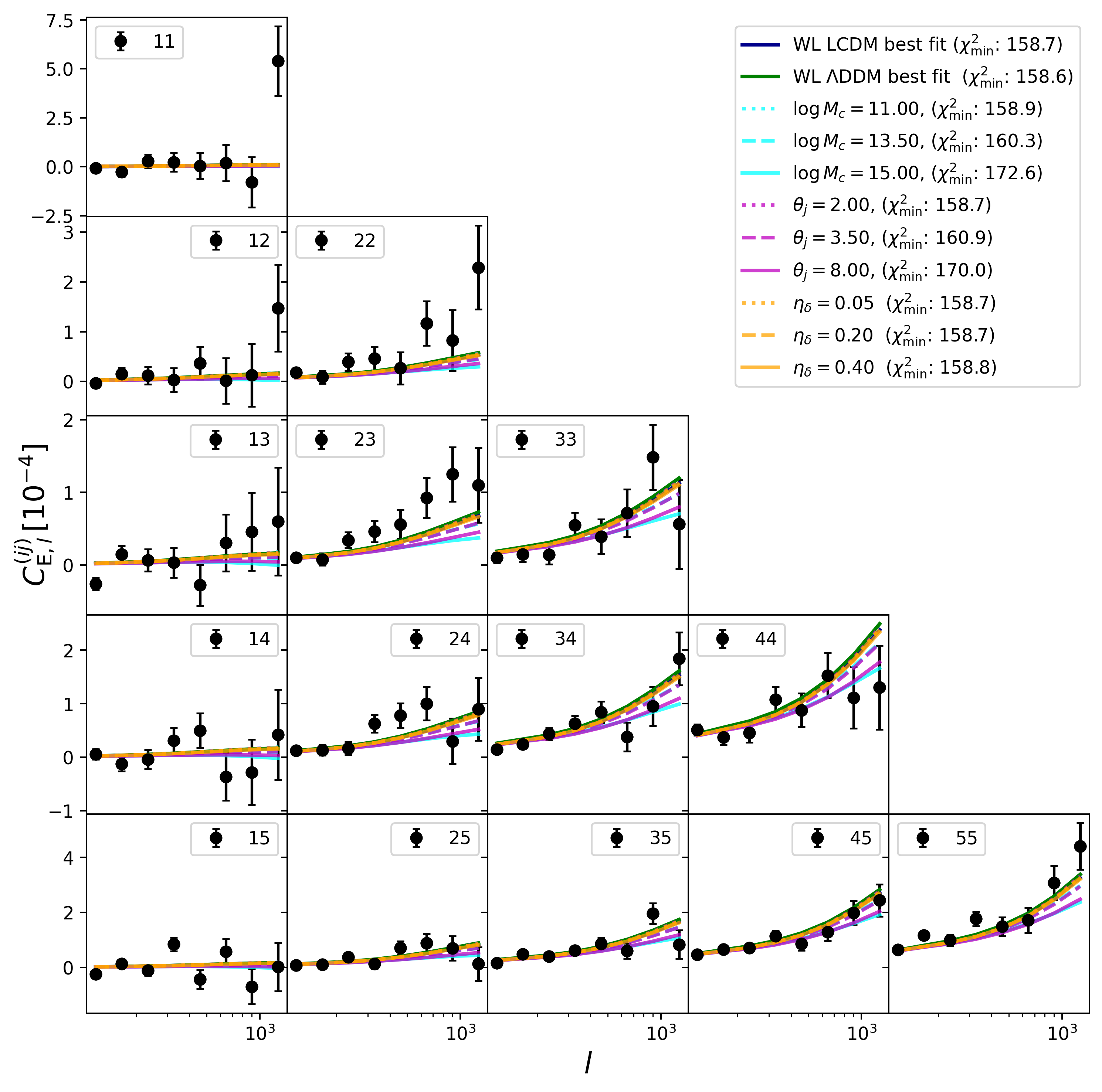
To correctly interpret results, it is important to understand the role of model parameters in relation to observables. Fig. 10 shows the original KiDS-1000 measurements of cosmic shear band powers with corresponding error bars (black points) and we illustrate how well WL, CMB and WL+CMB scenarios can fit these data. The solid green lines show the best fit configuration in the WL-only setup in the case of DDM (however, performing very similar to the CDM case). Once we calculate the band powers resulting from CMB-only best fit cosmology (orange lines), we recover significantly stronger WL signal compared to KiDS observations. This is the consequence of larger clustering ( value) preferred by CMB data. In the combined WL+CMB scenario, tighter error bars on cosmological parameters from Planck result in a best fit cosmology close to the one from the CMB-only scenario, but baryons and namely two-body decays on small scales provide a much better fit to cosmic shear data compared to the CMB-only scenario, as seen from the solid purple lines. To also showcase that two-body decays have a significant influence on the shear signal, we display the dashed and dotted purple lines. The former represents the same cosmology and baryonic parameters as in the solid purple case, but switching off the two-body decays completely, while the latter displays the largest possible impact of two-body decays in the case of cosmology and baryons fixed to the WL+CMB DDM best-fit scenario (solid purple lines). This impact is large enough to completely over- or underestimate the measured shear signal as can be seen e.g. from the autocorrelation spectra of higher-redshift bins. This also explains why in the case of combined DDM analysis, we recover the constraints on the two-body parameters that are detached from CDM cosmology.
In the combined WL+CMB scenario, the tighter error bars on cosmological parameters from the Planck results lead to a best-fit cosmology that is close to the one obtained from the CMB-only scenario. However, the inclusion of baryonic effects and, specifically, two-body decays on small scales improves the fit to the cosmic shear data, as indicated by the solid purple lines. To demonstrate the significant impact of two-body decays on the shear signal, we also display the dashed and dotted purple lines. The dashed line corresponds to the same cosmology and baryonic parameters as the solid purple case, but with two-body decays completely turned off. The dotted line represents the largest possible impact of two-body decays when the cosmology and baryons are fixed to the WL+CMB DDM best-fit scenario (solid purple lines). This impact is substantial enough to either overestimate or underestimate the measured shear signal, particularly noticeable in the autocorrelation spectra of higher-redshift bins. This explanation clarifies why, in the combined DDM analysis, we obtain constraints on the two-body parameters that are distinct from the CDM cosmology. The significant influence of two-body decays on the shear signal justifies the deviation from the CDM scenario.
C.2 Baryon feedback
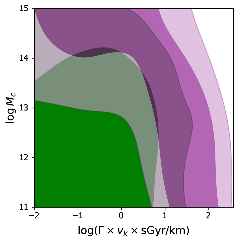
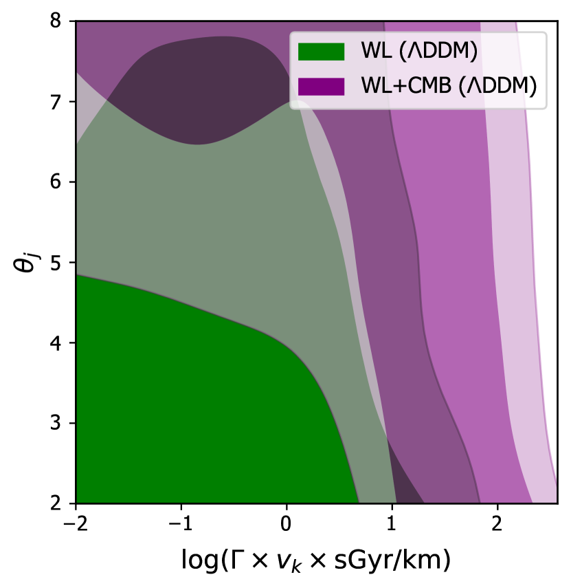
We use three free parameters in the baryonic effects emulator () as proposed in Giri & Schneider (2021). From our analysis, we find that the WL data does not provide any information about the stellar population parameter . This is evident from Fig. 11 and can be inferred from Tab. 4, as varying does not affect the modelled WL observables. On the other hand, the gas profile parameters and have an impact on the WL observables. For , we obtain for CDM (DDM) from the WL-only analysis, and from the combined analysis. Similarly, for , we find in the case of CDM (DDM) from the WL-only analysis, and from the combined analysis. These results indicate that the values of these baryonic parameters are mutually exclusive when comparing the WL-only and combined (CDM) scenarios. However, the underlying reasons for this behaviour are discussed in the following sections.
Fig. 11 demonstrates the impact of baryonic feedback on the KiDS band powers by varying the , and parameters within the BCemu framework. The best-fit configurations for CDM (DDM) are depicted in dark blue (green), while the coloured lines represent the variation of baryonic feedback strength in the CDM best-fit case. Notably, we observe that modifying the stellar population parameter does not alter the shear signal. However, adjustments to the gas profile parameters and affect the model predictions at scales .
Fig. 10 and 11 provide insights into how the baryonic and DDM parameters impact the band powers. Both sets of parameters exhibit a similar qualitative effect, resulting in a suppression of the signal at small scales. However, the influence of baryons is relatively subtle compared to the effects of DDM, as indicated by the available priors. Also, note that baryonic effects primarily manifest on the smallest scales, with no discernible impact below . In contrast, DDM can influence the signal on larger scales, particularly when considering scenarios with large velocity kicks.
Thus the analysis reveals that when considering KiDS data alone, the preferred values for baryonic feedback parameters (and in the DDM case, the two-body DDM parameters) tend towards the lower end. However, when combined with CMB data, these parameters drive the cosmology towards higher values, resulting in an excessive boost to the WL signal, as discussed earlier. The baryonic parameters can partially counteract this effect in the CDM scenario by decreasing the signal on small scales, which explains the extreme values observed for the gas profile parameters in the combined analysis with CMB. Nevertheless, the limited suppression capability of baryons is inadequate to fully accommodate the WL signal, leading to deteriorated fits for both WL and CMB.
In contrast, in the DDM scenario, the DDM parameters can more effectively suppress the band power signal, resulting in improved fits for both WL and CMB compared to the CDM setup. This can be observed in Fig. 12, where the left panel depicts the combination of DDM parameters with , and the right panel illustrates their combination with in the DDM model. In both panels, it is evident that fitting the WL-only data favours a weak suppression of the power spectrum, indicated by the green contours located in the bottom left region. Conversely, when combining WL and CMB, strong suppression is required either from baryons or from DDM, as indicated by the purple contours. It is conceivable that having even stronger baryonic effects at our disposal could entirely replace the need for DDM and provide a satisfactory fit to both data sets individually, though the physical justification for such high baryonic feedback remains an open question.
C.3 Cosmic Microwave Background
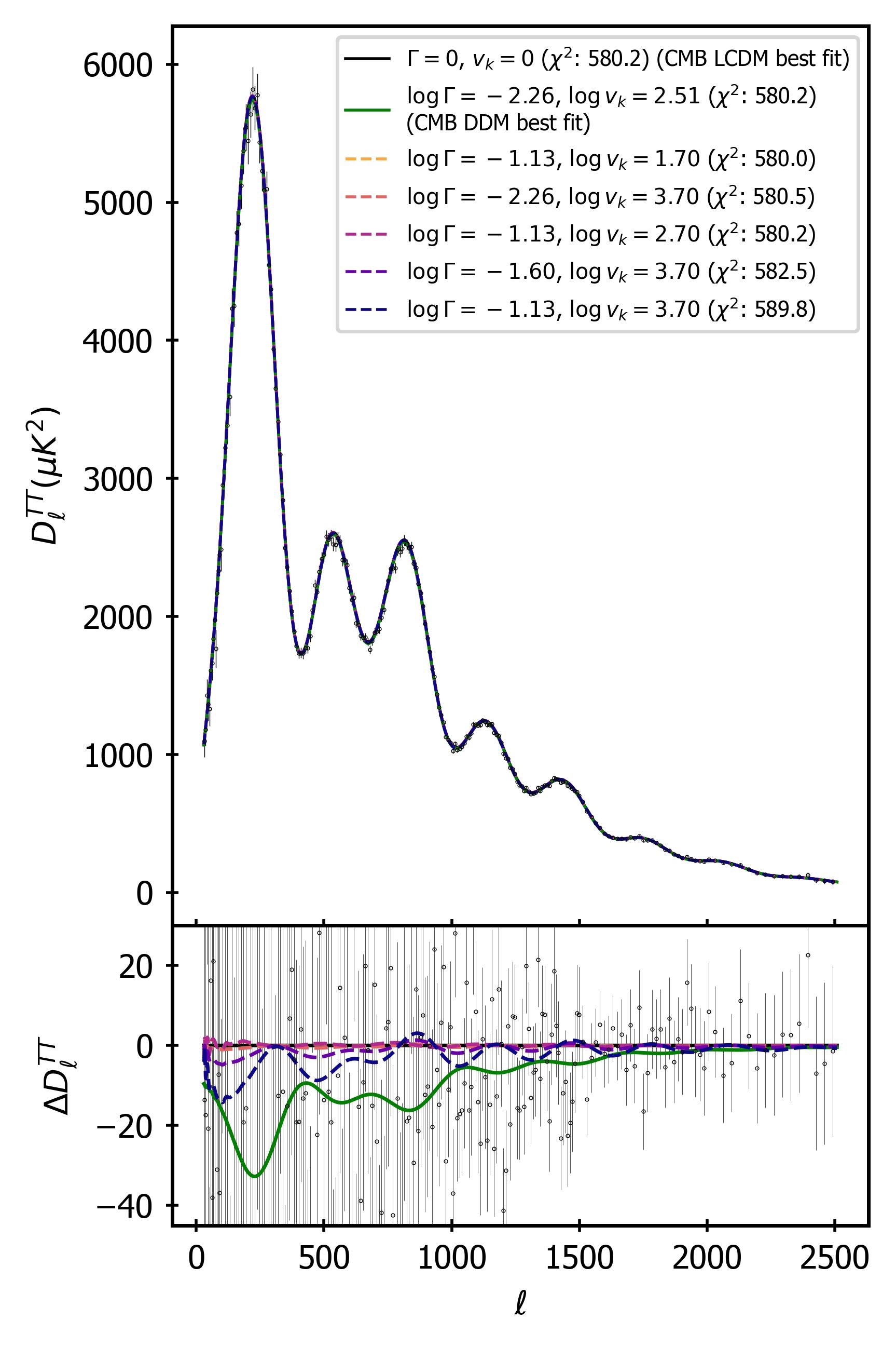
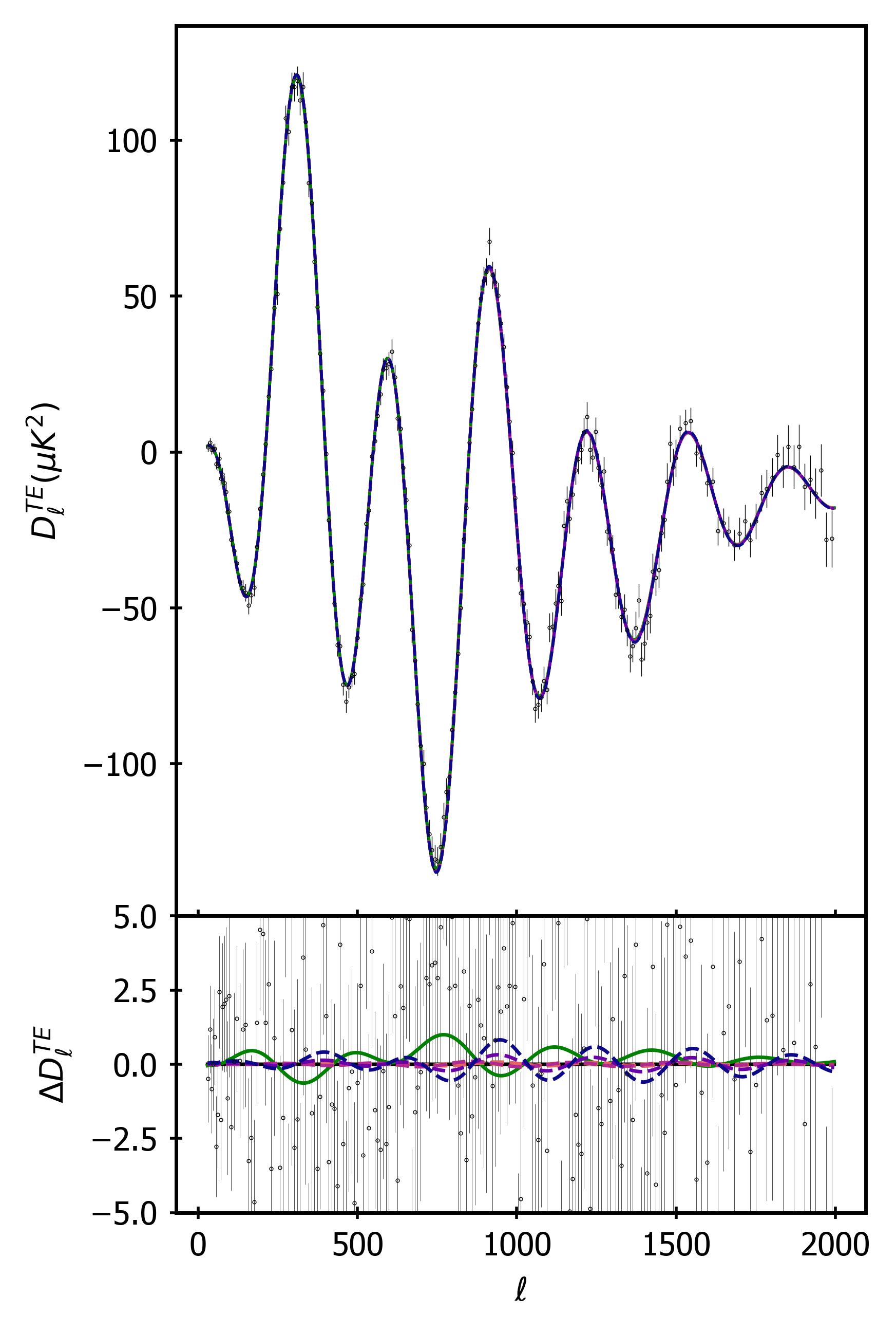
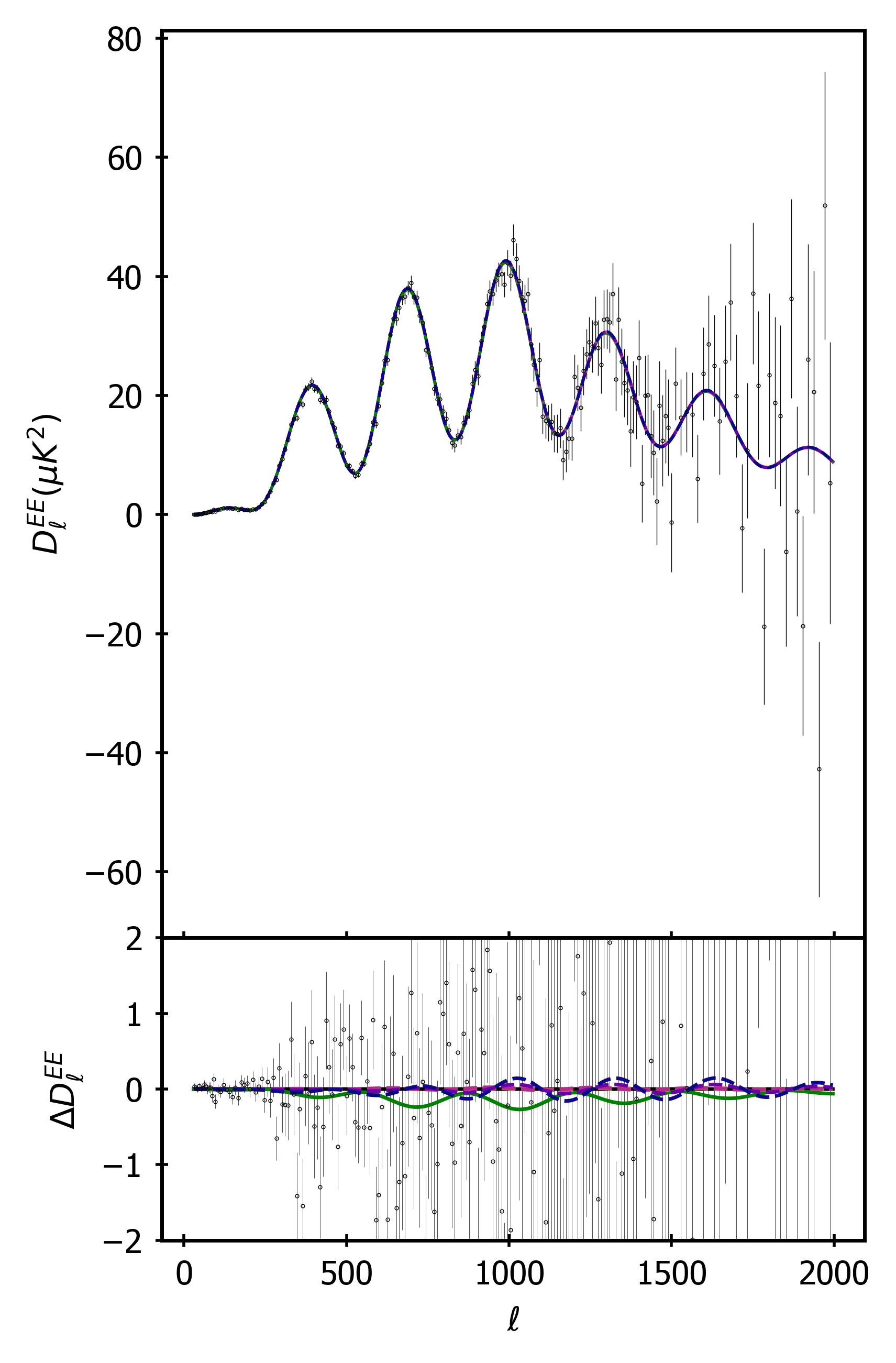
In Fig. 13 we show how two-body decays influence the predictions for CMB observables. We display temperature power spectra in the left and polarization spectra in the right panel and add their cross-correlations in the middle panel. In the top row, we show the CMB spectra for CDM (black) and DDM (green) best fits, while we plot the predictions for CDM best-fit configuration extended by different combinations of and (dashed lines). In the smaller bottom panels, we show the difference between all these predictions with the CDM best-fit cosmology. We can observe that two-body decays do not change the CMB signal significantly, meaning that the scatter of the CMB data is larger than the observable effects of two-body decays.
Appendix D Additional quantification of the tension
In the main text, we have introduced two different metrics to estimate tension within a model at hand, namely the Gaussian tension defined in Eq. (10) and Difference in maximum aposteriori following Eq. (11). The latter criterion is not subject to the assumption of Gaussian posteriors but cannot deal with over-fitting, i.e. how many additional degrees of freedom our new model possesses. The last criterion we use to assess the efficiency of the DDM model is the change in the Akaike information criterion (AIC) defined as
| (14) |
where is a number of free parameters in model . In order a new model is preferred over CDM, we require substantial evidence against it based on Jeffreys’ scale (Jeffreys 1961) using (Schöneberg et al. 2022), where . This implies that the difference in AIC () between the new model and CDM should satisfy the condition:
| (15) |
| WL | CMB | Combined | ||
|---|---|---|---|---|
| (CDM) | 158.7 | 580.2 | 750.5 | 3.4 |
| (DDM) | 158.6 | 580.2 | 742.6 | 1.9 |
| -0.1 | 0.0 | -7.9 | – | |
| 3.9 | 4.0 | -3.9 | – |
From the above equation we obtain and in the WL and CMB scenario, respectively, and this adding two free parameters does not lead to the improved fit to the data. In the combined scenario, . This means that the two additional parameters in the combined analysis are efficient. However, the combined DDM fit is still worse by compared to what DDM scenario yields when treating the two data sets separately. We believe that fitting the data separately provides a better indicator of resolving the tension, in which the DDM model fails. For a summary of combined MCMC results, we refer to Tab. 2.
Appendix E MCMC results
In this section, we provide more details about the parameters resulting from our MCMC analyses. In Tab. 3, we report our findings from CDM analysis (taken from Bucko et al. 2023), while in Tab. 4, we summarize the actual DDM model results. In both cases, we provide separate constraints from WL, CMB and combined analysis. In the upper part of the tables, we show the posteriors of the parameters sampled by MCMC, showing mean (best fit) values with corresponding upper and lower deviations. Dashed fields in the tables inform the parameters were not present in a given MCMC setup, unconst is used when parameters constraints could not be obtained from MCMC and we state no uncertainties whenever referring to a value constant throughout the inference.
| WL | CMB | WL + CMB | |
| Parameter | 68% limits | 68% limits | 68% limits |
| (prior) | |||
| ln() | |||
| ln() | |||
| WL | CMB | WL + CMB | |
| Parameter | 68% limits | 68% limits | 68% limits |
| ln(prior) | |||
| ln() | |||
| ln() | |||