The key role of Lagrangian multiplier in mimetic gravitational theory in the frame of isotropic compact star

Abstract

Recently, the mimetic gravitational theory has gained much attention in the frame of cosmology as well as in the domain of astrophysics. In this study, we show that in the frame of mimetic gravitation theory we are not able to derive an isotropic model. As a result, our focus shifts towards combining mimetic gravitational theory with the Lagrangian multiplier. The field equations of a static isotropic gravitational system that controls the geometry and dynamics of star structure are studied in the frame of mimetic theory coupled with a Lagrangian multiplier using a non-linear equation of state. An energy density is assumed from where all the other unknowns are fixed and a new isotropic model is derived. The physical analysis of this model is studied from different viewpoints and consistent results compatible with a realistic isotropic star are investigated analytically and graphically. Ultimately, we demonstrate the stability of the model in question by employing the adiabatic index technique.

I Introduction

Recently, conclusive evidence developed proposing that Einstein’s theory of general relativity (GR), is needy to be modified.The justifications for this observation stem from the challenges in renormalizing general relativity and the uncertain behavior exhibited in high gravity regions, such as the exterior of black holes and neutron stars. Additionally, the confirmed accelerated expansion of our universe can not be explained by GR. To be able to use GR to explain the phenomena of accelerated expansion of our universe an assumption of the presence of exotic matter fields like dark matter and dark energy must be taken into account. Up to date no experimental support for these was imminent. Another method is to try to amend Einstein’s GR somehow so that we keep its basic gains. Despite these issues in GR, it still submits success in the solar system. The success of the Event Horizon Telescope in capturing the image of a black hole’s shadow in M87 Akiyama et al. (2019) and the advancements made in detecting gravitational waves Abbott et al. (2016) have significantly bolstered the position of General Relativity as the preeminent gravitational theory compared to other theories of gravity. However, aspects that GR’s have not clarified must also face. We advocate the perspective that a modification of the governing field equations within the geometric sector holds the key to addressing these unresolved concerns.

Modified gravitational theories have made significant progress and performance in explaining some of the unsolved issues in GR. There are many modified theories of gravity that can overcome the shortcomings of GR. One of the modification of GR is to add a scalar field. In the frame of a scalar field coupled with Ricci scalar a static neutron star perspective using two types of cosmological inflationary attractor theories, i.e., the induced inflationary attractors and the quadratic inflationary attractors are investigated Oikonomou (2023a). Among these modification is the $f(R)$ gravitational theory (see for exmaple Nojiri et al., 2019; Odintsov and Oikonomou, 2019). In the frame of $f(R)$ a study of the neutron star phenomenology of $R^{p}$ attractor theories in the Einstein frame have been analyzed Oikonomou (2023b). In this study we are interested in another modification of GR, i.e., we are focused on the gravitational mimetic theory which has been suggested as a fresh approach to studying the problem of dark matter.Chamseddine and Mukhanov (2013). This concerns the introduction of a mimetic scalar field denoted as $\eta$, which, despite lacking dynamics in its construction, plays a crucial role in imparting dynamism to the longitudinal degree of freedom within the gravitational system. The gravitational system’s dynamic longitudinal degree serves as an analogue to pressureless dark matter, mimicking its properties Chamseddine and Mukhanov (2013). The problem of cosmological singularities Chamseddine and Mukhanov (2017a) and the singularity at the core of a black hole Chamseddine and Mukhanov (2017b) can be effectively tackled through the altered variant of mimetic gravitational theory. Furthermore, the gravitational theory of mimetic has substantiated that the propagation of gravitational waves at the speed of light aligns in perfect accordance with the discoveries made from the event GW170817 and the corresponding optical observations Casalino et al. (2018, 2019); Sherafati et al. (2021). Furthermore, it has been demonstrated that mimetic theory can explore the coherent rotational patterns observed in spiral galaxies without relying on the existence of dark matter particles Vagnozzi (2017); Sheykhi and Grunau (2021). Lately, there has been a significant surge of enthusiasm surrounding the cosmological framework due to the emergence of the mimetic theory Chamseddine et al. (2014); Baffou et al. (2017); Dutta et al. (2018); Sheykhi (2018); Abbassi et al. (2018); Matsumoto (2016); Sebastiani et al. (2017); Sadeghnezhad and Nozari (2017); Gorji et al. (2019, 2018a); Bouhmadi-Lopez et al. (2017); Gorji et al. (2018b); Chamseddine et al. (2019a); Russ (2021); de Cesare et al. (2020); Cárdenas et al. (2021); Hosseini Mansoori et al. (2021); Arroja et al. (2018) and black holes physics Deruelle and Rua (2014); Myrzakulov and Sebastiani (2015); Myrzakulov et al. (2016); Ganz et al. (2019); Chen et al. (2018); Nashed (2018b); Ben Achour et al. (2018); Brahma et al. (2018); Zheng et al. (2017); Shen et al. (2019); Nashed et al. (2019); Chamseddine et al. (2019b); Gorji et al. (2020); Sheykhi (2020, 2020); Nashed and Nojiri (2021); Chamseddine (2021); Zheng (2021); Bakhtiarizadeh (2021); Nashed (2021). The theory has further extended its scope to include $f(R)$ mimetic gravity, incorporating additional insights and explanations Nojiri and Odintsov (2014); Odintsov and Oikonomou (2016a); Oikonomou (2016a, b, c); Myrzakulov and Sebastiani (2016); Odintsov and Oikonomou (2015, 2016b, 2016c); Nojiri et al. (2017); Odintsov and Oikonomou (2018); Bhattacharjee (2021); Kaczmarek and Szczesniak (2021); Chen et al. (2021) and mimetic Gauss-Bonnet gravity Astashenok et al. (2015); Oikonomou (2015); Zhong and Elizalde (2016); Zhong and Sáez-Chillón Gómez (2018); Paul et al. (2020). Specifically, a comprehensive framework combining early inflation and late-time acceleration within the context of mimetic $f(R)$ gravity was formulated Nojiri et al. (2016). It has been stressed that within the context of mimetic $f(R)$ gravity, the period of inflation can be identified Nojiri et al. (2016).

Nowadays, the mimetic theory is one of the most compelling theories of gravity, which without introducing any additional field of matter, represents the dark side of the universe which is represented as a geometric effect. The observations ensure that approximately 26$\%$ of the energy content of the universe is related to the dark matter sector, while approximately 69$\%$ construct the dark energy Yang and Gong (2020). Many facts ensure the presence of dark matter and dark energy Seljak et al. (2006). Dark energy, which has gained significance in recent times, is believed to be a smooth element characterized by negative pressure. It possesses an anti-gravity characteristic and is actively propelling the universe, playing a key role in the accelerated expansion of the cosmos Oks (2021). Dark matter performs two crucial functions in the development of the universe: Firstly, it provides the necessary gravitational force for the rotation of spiral galaxies and galaxy clusters. Secondly, it plays a significant role as an essential component in the amplification of disturbances and the formation of structures during the early stages of the universe. As a result, dark matter begins to condense into an intricate system of dark matter halos, whereas regular matter undergoes collapse due to photon radiation, eventually settling into the well-formed potential of dark matter. In the absence of dark matter, the process of galaxy formation in the universe would be significantly more extensive than what has been observed.

The structure of the current investigation is outlined as: In Sec. II, we introduce the fundamental principles of the mimetic theory combined with the Lagrangian multiplier. In Sec. III, we list the necessary conditions that must be obeyed by any realistic isotropic model. Also, in Sec.n III we show that the model under consideration satisfies all the necessary conditions, analytically and graphically, that must possess by any realistic isotropic star. In Section IV we study the stability of the model presented in this study using the adiabatic index. Final Section is devoted to discussing the main results of the present study.

II Isotropic solution in the mimetic theory combined with the Lagrange multiplier

What is called “dark matter of mimetic” was delivered in the scientific society in Chamseddine et al. (2014). Despite of this mimetic theories had already been discussed in Lim et al. (2010); Gao et al. (2011); Nashed and Saridakis (2023); Nashed and Nojiri (2022); Nashed (2021); Nashed and Nojiri (2021); Nashed (2018a); Nashed et al. (2019); Nashed (2018b); Capozziello et al. (2010); Sebastiani et al. (2017).

According to the theory of mimetic, the metric $g_{\alpha\beta}$, which is a physical one, is linked to the metric $\bar{g}_{\alpha\beta}$, which is an auxiliary metric, and to the mimetic scalar field $\eta$ by the conformal transformation:

$$g_{\alpha\beta}=-\left(\bar{g}^{\mu\nu}\partial_{\mu}\eta\partial_{\nu}\eta\right)\bar{g}_{\alpha\beta}\,,$$ (1)

where the metric $\bar{g}^{\alpha\beta}$ undergoes conformal transformations, specifically $\bar{g}^{\alpha\beta}\to\Omega\bar{g}^{\alpha\beta}$, the metric $g^{\alpha\beta}$ remains invariant, meaning that it remains unchanged.

In the present study, we will coin the mimetic-like gravity coupled with the Lagrange multiplier. The action of the gravity model resembling the mimetic theory, in conjunction with the Lagrange multiplier $\lambda$ and the function $\omega$, is described as follows: has the form Nojiri and Odintsov (2014):

$$S=\int\mathrm{d}x^{4}\sqrt{-g}\left\{R+\lambda\left(g^{\mu\nu}\omega\partial_{\mu}\eta\partial_{\nu}\eta+1\right)\right\}+L_{\mathrm{matt}}\,,$$ (2)

where $L_{\mathrm{matt}}$ is the Lagrangian of the matter field and $\eta$ is the mimetic scalar field. The field equations can be obtained by taking the variation of the action (2) with respect to the metric tensor $g_{\mu\nu}$, resulting in the following expressions:

$$0=R_{\mu\nu}-\frac{1}{2}g_{\mu\nu}R+\frac{1}{2}g_{\mu\nu}\left\{\lambda\left(g^{\rho\sigma}\omega\partial_{\rho}\eta\partial_{\sigma}\eta+1\right)\right\}-\lambda\partial_{\mu}\eta\partial_{\nu}\eta+\frac{1}{2}T_{\mu\nu}\,,$$ (3)

where $T_{\mu\nu}$ is the energy-momentum tensor corresponding to the matter field. Additionally, differentiating the action (2) with respect to the mimetic field $\eta$ yields:

$$2\nabla^{\mu}(\lambda\omega\,\partial_{\mu}\eta)=0\,.$$ (4)

When the action (2) is varied with respect to the Lagrange multiplier $\lambda$, the following outcome is obtained:

$$g^{\rho\sigma}\omega\partial_{\rho}\eta\partial_{\sigma}\eta=-1\,.$$ (5)

It is the time to apply the field equations (3) and (4), using the constrains of Eq. (5), to the following spherically symmetric spacetime

$$ds^{2}=f(r)dt^{2}-\frac{dr^{2}}{f_{1}(r)}-r^{2}\left(d\theta^{2}+r^{2}\sin^{2}\theta d\phi^{2}\right)\,,$$ (6)

to derive an interior solution. The functions $f(r)$ and $f_{1}(r)$ mentioned here are unfamiliar functions that will be determined by solving the set of field equations.

Furthermore, we assume that $\eta$ is solely dependent on $r$. Using Eqs. (3) and (4) to the spacetime (6), yields the following set of differential equations. The $(t,t)$-component of the field equation (3) is:

$$\rho(r)= \frac{1-f_{1}-rf^{\prime}_{1}}{r^{2}}\,,$$ (7)

the field equation (3) can be expressed as the $(r,r)$-component.

$$p(r)= \frac{f_{1}f^{\prime}r-f+ff_{1}-\lambda\omega(r)\eta^{\prime 2}ff_{1}r^{2}}{r^{2}f}\,,$$ (8)

the components of the field equation (3) in terms of $(\theta,\theta)$ and $(\phi,\phi)$ have the following structure:

$$p(r)= \frac{2\,f_{1}f^{\prime\prime}fr-f^{\prime 2}f_{1}r+f\left(2\,f_{1}+f^{\prime}_{1}r\right)f^{\prime}+2\,f^{\prime}_{1}f^{2}}{4f^{2}r}\,,$$ (9)

and the field equation (4) takes the form:

$$0=2\lambda^{\prime}\omega fr+\left[\omega^{\prime}fr+\omega\left(f^{\prime}r+4\,f\right)\right]\lambda\,,$$ (10)

where $f\,\equiv f(r)$, $f_{1}\,\equiv f_{1}(r)$, $\omega\,\equiv\omega(r)$, $\lambda\,\equiv\lambda(r)$, $f^{\prime}=\frac{df}{dr}$, $f^{\prime}_{1}=\frac{df_{1}}{dr}$, $\eta^{\prime}=\frac{d\eta}{dr}$, $\omega^{\prime}=\frac{d\omega}{dr}$, and $\lambda^{\prime}=\frac{d\lambda}{dr}$. Furthermore, we make the assumption that the energy-momentum tensor of the isotropic fluid can be represented in the following manner:

$${T}_{\mu\nu}=(\rho+p)u_{\mu}u_{\nu}+pg_{\mu\nu}\,,$$ (11)

In this case, $\rho$ represents the energy density, $p$ denotes the pressure, and $u^{\mu}$ is a timelike vector defined as $u^{\mu}=[1,0,0,0]$.In this particular investigation, we consider the matter content to be characterized by the energy density $\rho$ and the pressure $p$ respectively..

Assuming the fluid under consideration has a perfect fluid verifying the equation of state (EoS), $p=p\left(\rho\right)$. Using the conservation law of matter gives:

$$0=\nabla^{\mu}\,T_{\mu r}=2f\frac{dp}{dr}+f^{\prime}\left(\rho+p\right)\,.$$ (12)

In this particular context, we make an assumption that the energy density and pressure of the system exhibit variations based on the radial coordinate.

If the form of EoS $\rho=\rho(p)$ is presented, then Eq. (12) yield:

$$\frac{1}{2}\ln f=-\int^{r}dr\frac{\frac{dp}{dr}}{\rho+p}=-\int^{p(r)}\frac{dp}{\rho(p)+p}\,.$$ (13)

In the interior of the star, Eq. (13) can be used but in the exterior, Eq. (13) cannot be used. Nevertheless, it is possible to assume that both $f(r)$ and its derivative $f^{\prime}(r)$ exhibit continuity at the surface of the star.

Considering the count of unknown functions and independent equations, we find a total of six unknown functions within the compact star. To address this, we will employ the constraint given by Eq. (5), which states that $\eta=\frac{1}{\sqrt{-\omega f_{1}}}$. These unknown functions include two metric potentials, namely $f(r)$ and $f_{1}(r)$ in (6), as well as the Lagrangian multiplier, the function $\omega$, the energy density $\rho$, and the pressure $p$ present in the action (2). However, we have 3 independent equations, that are, the three components, Eqs. (7), (8), and (9) of the field equation (3) of the mimetic equations, an equation of state $\rho=\rho(p)$, and the conservation law (12). As we mentioned above, the scalar field equation (4) can be obtained from the field equations (3) corresponding to the mimetic equation and the conservation law $\nabla_{\mu}T^{\mu\nu}=0$ of the matter, and therefore the scalar field equation (4) is not independent. Hence, we have $6-5=1$ undetermined function remaining from the equations. To address this remaining aspect, we opt for the specific configuration of energy density $\rho=\rho(r)$ within the compact celestial object. Moreover, outside the star, we have $\rho=p=0$, and the unknown functions, $f(r)$, $f_{1}(r)$ and $\eta$ (or $\omega(\eta)$). We have 3 independent equations, that are, the three components, Eqs. (7), (8), and (9). Thus there are $5-4=1$ function undetermined from the equations, again.

If we consider a compact star like neutron star, one usually consider the EoS as:

1. Energy-polytrope

   $$p=k\rho^{1+\frac{1}{s}}\,,$$ (14)

   where $k$ and $s$ are constants. It is well known that for neutron star, $s$ lies in the interval $s\in[0.5\,,\,1]$.

2. Mass-polytrope

   $$\rho=\rho_{m}+s_{1}p\,,\qquad\qquad p=m_{m}\rho_{m}^{1+\frac{1}{s_{m}}}\,,$$ (15)

   with $\rho_{m}$ being the rest mass energy density and $m_{m}$, $s_{1}$, and $s_{m}$ are constants.

Now, let us turn our attention to the study of the energy-polytrope case. Then EoS (14) can be rewritten as:

$$\rho=\tilde{k}p^{({1+\frac{1}{\tilde{s}}})}\,,\quad\tilde{k}\equiv k^{-\frac{1}{1+\frac{1}{s}}}\,,\quad\tilde{s}\equiv\frac{1}{\frac{1}{1+\frac{1}{s}}-1}=-1-s\,.$$ (16)

Eq. (13) can take the form:

$$\frac{1}{2}\ln f=-\int^{p(r)}\frac{dp}{\tilde{k}p^{1+\frac{1}{\tilde{s}}}+p}=\frac{c_{1}}{2}+\tilde{s}\ln\left(1+{\tilde{k}}^{-1}p^{-\frac{1}{\tilde{s}}}\right)=\frac{c_{1}}{2}-\left(1+s\right)\ln\left(1+k\rho^{\frac{1}{s}}\right)\,,$$ (17)

where $c_{1}$ is a constant of integration. Using the same method of polytrope we get for mass-polytrope (15) the function $f$ as:

$$\frac{1}{2}\ln f=\frac{\tilde{c}}{2}+\ln\left(1-k_{m}\rho_{m}{}^{\frac{1}{s_{m}}}\right)\,,$$ (18)

where $\tilde{c}$ is a constant of integration.

To provide an illustrative example, taking into account one of the mentioned equations of state, we can make an assumption about the profile of $\rho=\rho(r)$ as follows.

$$\rho=\left\{\begin{array}[]{cc}\rho_{0}\left(1-\frac{r}{{R}}\right)&\ \mbox{when}\ r<R\\ 0&\ \ \mbox{when}\ r\geq R\end{array}\right.\,.$$ (21)

In this scenario, $\rho_{0}$ represents a fixed value expressing the energy concentration at the core of the condensed celestial object, whereas $R$ symbolizes an additional fixed value denoting the size of the compact star’s outer boundary. As clear from Eq. (21), the energy density $\rho$ vanishes at the surface $r=R$. By using the energy-polytrope EoS (14) or the mass-polytrope EoS (15), we find that the pressure $p$ also vanishes at the surface. We have introduced the mass parameter $M$ as a constant value, which is associated with the mass of the compact star. This parameter is defined specifically for the polytropic equation of state (EoS) as follows:

$$M=4\pi\int_{0}^{R}y^{2}\rho(y)dy=\frac{\pi\rho_{0}R^{3}}{3}\,.$$ (22)

Then Eq. (17) gives,

$$f=\frac{\mathrm{e}^{c_{1}}}{\left(1+k\rho_{0}\left(1-\frac{r}{{R}}\right)\right)^{4}}\,.$$ (23)

Using Eq. (21) in (7) we get:

$$f_{1}=1-\frac{8\pi r^{2}}{3}+\frac{2r^{3}}{R}\,.$$ (24)

The Lagrangian multiplier of the above model has the form

$$\lambda(r)= \frac{c_{2}\,\left(R+kR-kr\right)^{2}}{{r}^{5/2}}\,.$$ (25)

To finalize the determination of the remaining unknowns we assume, for simplicity, the form of the function $\omega=c_{3}r$ and the mimetic scalar field becomes:

$$\eta(r)= \sqrt{c_{3}r\left(\frac{8\pi r^{2}}{3}-\frac{2r^{3}}{R}-1\right)}\,.$$ (26)

To finalize this section we stress on the fact that if we follow the same procedure and put $\lambda(r)=0$ in Eqs. (7), (8), and (9) we get a system that we cannot derive from it an isotropic model.

III Necessary conditions for a real physical star

Any physical reliable isotropic star model must obey the below conditions in the interior configurations:
$\bullet$ It is essential for the metric potentials ($g_{tt}$ and $g_{r}r$) to provide precise explanations for the density and momentum components by establishing unambiguous definitions and displaying consistent patterns within the core of the star and its interior.
$\bullet$ Within the interior of the star, it is required that the energy density $\rho$ maintains a non-negative value, that is, $\rho\geq 0$. Additionally, the energy density has a finite positive value at the central region of the star and shows a decreasing pattern as it extends towards the surface, characterized by the condition $\frac{d\rho}{dr}\leq 0$.
$\bullet$ Inside the fluid configuration, it is necessary for the pressure $p$ to be positive or zero ($p\geq 0$). Furthermore, within the interior of the star, it is expected that the pressure decreases with respect to the radial coordinate, as indicated by the condition $\frac{dp}{dr}<0$. On the outermost boundary of the star, specifically at the surface where the distance from the center is denoted as $r=R$, the pressure $p$ should be precisely zero. This implies that there is no pressure exerted at the star’s outer edge.
$\bullet$ The energy conditions of an isotropic fluid sphere are given by:
(i) The null energy condition (NEC) implies that the energy density $\rho$ must be greater than zero.
(ii) According to the weak energy condition (WEC), the sum of the pressure $p$ and the energy density $\rho$ must be greater than zero, i.e., $p+\rho>0$.
(iii) In accordance with the strong energy condition (SEC), the sum of the energy density $\rho$ and three times the pressure $p$ must be greater than zero, i.e., $\rho+3p>0$.
$\bullet$Furthermore, to ensure a realistic model, the causality condition must be satisfied within the interior of the star. This condition imposes a restriction on the speed of sound, requiring it to be less than 1. In this context, assuming the speed of light $c$ is equal to 1, the condition can be expressed as $\frac{dp}{dr}>0$ and $1>\frac{dp}{dr}$.
$\bullet$ Finally, the adiabatic index must has a value more than $\frac{4}{3}$.

It is our purpose to study the above conditions on the isotropic model and see if it is real model or not.

IV The physical characteristics of the model

To determine whether the model described by Eqs. (17), (21), and (24) corresponds to a realistic stellar structure, we will examine the following aspects:

IV.1 Non singular model

i- The components of the metric potentials $g_{tt}$ and $g_{rr}$ fulfill the following conditions:,

$$f(x\rightarrow 0)=\frac{e^{c}}{(1+k\rho_{c})^{4}}\,\qquad\textrm{and}\qquad f_{1}(x\rightarrow 0)=1.$$ (27)

As a consequence of this requirement, it is necessary for the metric potentials $g_{tt}$ and $g_{rr}$ to possess finite values at the central point of the stellar configuration. Furthermore, their derivatives also possess finite values at the center of the star, specifically: $a^{\prime}(r\rightarrow 0)=0$ and $a^{\prime}_{1}(r\rightarrow 0)=\frac{4c_{1}k}{R(1+k)^{5}}$. The mentioned limitations guarantee that the measurement remains consistent at the core and demonstrates a positive characteristic within the inner region of the star.
ii-At center of star, the density (21) and pressure (14) take the following form:

$$\rho(x\rightarrow 0)=\rho_{0}\,\qquad p(x\rightarrow 0)=k\rho_{0}{}^{2}.$$ (28)

By examining Eq. (28), when $\rho_{0}>0$ and $k>0$, it becomes evident that the density and pressure in the central region of the star remain consistently positive. Apart from that, if $\rho_{0}$ or $k$ is non-positive, the density and pressure can become negative. These observations align with the information depicted in Figures 1 0(a), 1 0(b), and 1 0(c), providing further consistency to the discussed aspects.
iii-The density and pressure gradients of our model are provided in the following manner:

$$\rho^{\prime}=-\rho_{0},\qquad\qquad p^{\prime}=-{2k\rho_{0}{}^{2}\,(1-x)}\,.$$ (29)

Here $\rho^{\prime}=\frac{d\rho}{dx}$ and $p^{\prime}=\frac{dp}{dx}$. Equation (29) illustrates that the components of the energy-momentum derivatives exhibit negative values.
iv-The calculation of the speed of sound, using relativistic units where the values of $c$ and $G$ are equal to 1, is achieved by Herrera (1992):

$$v_{r}{}^{2}=\frac{dp}{d\rho}=2\,k\,\rho_{0}\,(1-x)\,.$$ (30)

At this point, we are prepared to graphically represent the aforementioned conditions in order to observe their behaviors. In Figure 1 0(a), we illustrate the characteristics of the metric potentials. As depicted in Figure 1 0(a), the metric potentials take on the values $a_{1}(x\rightarrow 0)=0.4$ and $a(x\rightarrow 0)=1$ as $x$ approaches 0. This implies that within the central region of the star, both metric potentials exhibit finite positive values.

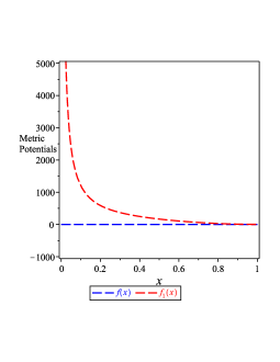
(a)  Metric potentials, $f(r)$ and $f_{1}(r)$ given by Eq. (23) and (24)

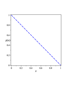
(b)  Density

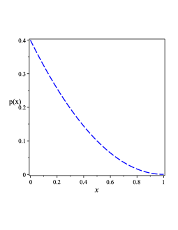
(c)  Pressure

Figure 1: A visual representation is provided, illustrating the relationship between the metric potentials (23) and (24), in comparison to the dimensionless x; 0(b) the profile of density; and 0(c) profile of pressure. We have put $\rho_{0}=1$ and $K=0.4$.

We proceed to create graphs illustrating the density and pressure, as outlined in Equation (21), represented in Figure 1 0(b) and 1 0(c). As depicted in Figure 1 0(b) and 1 0(c), the components of the energy-momentum exhibit positive values, which are consistent with predictions for a reasonable stellar arrangement. Moreover, as depicted in Figure 1 0(b) and 0(c), the components of the energy-momentum tensor exhibit elevated values at the core and gradually decrease as they approach the periphery. These observed patterns are characteristic of a plausible star.

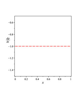
(a)  Gradient of density

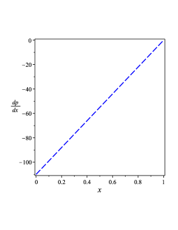
(b)  Gradient of pressure

Figure 2: A graph is shown, displaying the variations in the gradient of density and pressure from Equation (21), plotted against the dimensionless value of $x$.

Figure 2 illustrates the presence of adverse values in the derivatives of the components of the energy-momentum tensor, indicating a uniform decrease in both density and pressure throughout the entirety of the star’s structure.

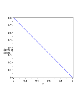
(a)  Sound speed

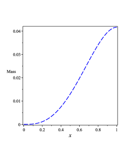
(b)  Relationship between mass and radius

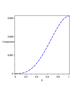
(c)  The compactness

Figure 3: A diagram is presented, depicting the behavior of various quantities with respect to the dimensionless value of $x$. Specifically, the plot includes the sound speed (labeled as 2(a)), the relation between mass and radius (labeled as 2(b)), and the level of compactness exhibited by the celestial body(labeled as 2(c)).

Figure 3 presents visual depictions of the speed of sound, the relationship between mass and radius, and the compactness parameter. As depicted in Fig. 32(a), the speed of sound is found to be less than one, which verifies that the causality condition is not violated within the interior of the stellar configuration when the parameter of the equation of state (EoS) is $k<0.5$. Furthermore, Fig. 32(c) illustrates that the compactness of our model is restricted within the interval of $0<C<0.003$, where $C$ is defined as the ratio of $M$ to $xR$ in the stellar arrangement.

(a)  Null energy conditions

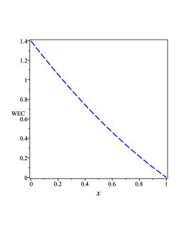
(b)  Weak energy conditions

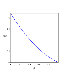
(c)  Strong energy condition

Figure 4: A graph is generated to illustrate the behavior of the null, weak, and strong energy conditions, as determined by Equation (21), plotted against the dimensionless value of $x$.

The energy conditions are depicted in Figure 4, showcasing the characteristics of each condition. More specifically, Fig. 4 3(a), 3(b), and 3(c) display the presence of positive values for the NEC (Null Energy Condition), WEC (Weak Energy Condition), and SEC (Strong Energy Condition) respectively. This verification provides assurance that all energy conditions are met across the entire stellar configuration, aligning with the criteria for a physically feasible stellar model.

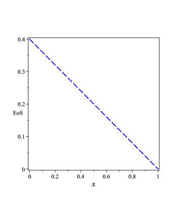
Figure 5: A plot is presented to visualize the equation of state (EoS) as a function of the radial coordinate $r$, labeled as 5. Additionally, the redshift is plotted and labeled as 5.

Figure 5 represents the plot of the Equation of State (EoS). In particular, Figure 5 5 indicates that the EoS exhibits a linear behavior.

V The model’s stability

At this point, we are prepared to examine the stability concern of our model by conducting tests involving the the index of adiabatic and the static case.

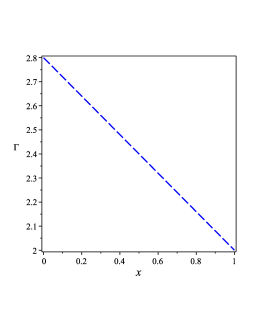
Figure 6: Plot of the gravitational, and the hydrostatic forces vs. the dimensionless $x$.

V.1 An adiabatic index

To investigate the stable balance of a spacetime that possesses spherical symmetry, an analysis of the adiabatic index can be conducted. The adiabatic index plays a vital role in evaluating the stability requirement, serving as an essential instrument for this purpose. Specifically, the adiabatic perturbation, denoted as $\Gamma$, is defined as follows Chandrasekhar (1964); Merafina and Ruffini (1989); Chan et al. (1993); Nashed (2011); Nashed and Capozziello (2021); Nashed (2011); Nashed and Capozziello (2020); Roupas and Nashed (2020):

$$\Gamma=\left(\frac{\rho+p(x)}{p(x)}\right)\left(\frac{dp(x)}{d\rho(x)}\right)\,.$$ (31)

If the adiabatic index $\Gamma$ is greater than $\frac{4}{3}$, a Newtonian isotropic sphere will have a stable equilibrium Heintzmann and Hillebrandt (1975).

Using Eq. (31), we get

$$\Gamma=2+2k\rho_{0}(1-x).$$ (32)

Figure 6 displays the adiabatic index $\Gamma$. The graph clearly indicates that the value of $\Gamma$ remains consistently above $4/3$ throughout the star’s interior. Therefore, we can infer that the stability requirement is met.

V.2 Stability in the stationary state

Another approach to validate the stability of model (21) involves investigating the static state proposed by Harrison, Zeldovich, and Novikov Harrison et al. (1965); Zeldovich and Novikov (1971, 1983). In a previous study by Harrison, Zeldovich, and Novikov, it was established that a stable configuration of a star necessitates a positive and increasing derivative of mass with respect to the central density $\rho(x\rightarrow 0)$, denoted as $\frac{\partial M}{\partial\rho_{0}}>0$. By applying this condition, we can determine the specific form of the central density as follows:

$$\rho(r\to 0)=\rho_{0}\,.$$ (33)

Subsequently, utilizing Eq. (22), we can derive the mass corresponding to the central density, denoted as:

$$M(\rho_{0})4\pi\int_{0}^{R}y^{2}\rho(y)dy=\frac{\pi\rho_{0}R^{3}}{3}\,.$$ (34)

The behavior of the mass derivative with respect to the central density can be described by the following pattern:

$$\frac{\partial M(\rho_{0})}{\partial\rho_{0}}=\frac{\pi R^{3}}{3}\,.$$ (35)

Equations (34) and (35) guarantee the verification of stability condition of our model.

VI Discussion and conclusions

The primary objective of this investigation is to analyze a compact star’s static configuration, which possesses both spherical symmetry and is within the framework of mimetic gravity theory. This theory incorporates two main components: a scalar field and a Lagrangian multiplier. In our formulation, we demonstrated the ability to construct a model that accurately replicates the profile of a given spherically symmetric spacetime, regardless of the equation of state (EoS) for matter and energy density. The shape of the density function $\rho(x)$ is of utmost importance in determining the radius $R$ and mass $M$ of the compact star. By manipulating the Lagrangian multiplier $\lambda(\eta)$, it becomes feasible to establish a flexible connection between the radius $R$ and the compact star. This creates a situation where the Lagrangian multiplier $\lambda(x)$ and the equation of state (EoS) describing the model exhibit a degenerate relationship. As a result, it is clear that relying solely on the mass-radius relation is inadequate for fully constraining the model.

To illustrate this further, we take a closer look at the polytrope equation of state (EoS) given by (14). By selecting a specific form for the density in Eq.  (21), we construct a practical isotropic model. We then proceed to investigate the physical characteristics of this model. Through rigorous analysis using different analytical techniques and validations, we carefully scrutinize the obtained analytic solution. This comprehensive examination enables us to observe and analyze the physical behavior manifested by our solution.

It is important to highlight that the preceding discussion confirms the satisfaction of all the physical conditions by the spherically symmetric interior spacetime configuration considered in this study within the framework of mimetic gravitational theory coupled with a Lagrangian multiplier. However, it should be noted that an alternative form of mimetic gravitational theory that does not involve the coupling with a Lagrangian multiplier may not support the existence of the isotropic model, as evidenced by equations (7), (8), and (9).

Moreover, the field equations governing the equilibrium of rapidly rotating neutron stars in scalar-tensor theories of gravity, as well as representative numerical solutions are discussed in Doneva et al. (2013). New models of slowly rotating, perfect-fluid neutron stars are constructed by extending the classical Hartle-Thorne formalism to generic scalar-tensor theories of gravity Pani and Berti (2014). An investigation of self-consistently slowly rotating neutron and strange stars in R-squared gravity is investigated in Staykov et al. (2014). A study of static neutron stars in the framework of a class of non-minimally coupled inflationary potentials have been presented in Oikonomou (2021). Are all the previous studies presented in Doneva et al. (2013); Pani and Berti (2014); Staykov et al. (2014); Oikonomou (2021) can be discussed in the framework of the present study? This will be done elsewhere.

References

- Akiyama et al. (2019) K. Akiyama et al. (Event Horizon Telescope), Astrophys. J. Lett. 875, L1 (2019), arXiv:1906.11238 [astro-ph.GA] .
- Abbott et al. (2016) B. P. Abbott et al. (LIGO Scientific, Virgo), Phys. Rev. Lett. 116, 061102 (2016), arXiv:1602.03837 [gr-qc] .
- Oikonomou (2023a) V. K. Oikonomou, Class. Quant. Grav. 40, 085005 (2023a), arXiv:2303.06270 [gr-qc] .
- Nojiri et al. (2019) S. Nojiri, S. D. Odintsov, and V. K. Oikonomou, Nucl. Phys. B 941, 11 (2019), arXiv:1902.03669 [gr-qc] .
- Odintsov and Oikonomou (2019) S. D. Odintsov and V. K. Oikonomou, Class. Quant. Grav. 36, 065008 (2019), arXiv:1902.01422 [gr-qc] .
- Oikonomou (2023b) V. K. Oikonomou, Mon. Not. Roy. Astron. Soc. 520, 2934 (2023b), arXiv:2301.12136 [gr-qc] .
- Chamseddine and Mukhanov (2013) A. H. Chamseddine and V. Mukhanov, JHEP 11, 135 (2013), arXiv:1308.5410 [astro-ph.CO] .
- Chamseddine and Mukhanov (2017a) A. H. Chamseddine and V. Mukhanov, JCAP 1703, 009 (2017a), arXiv:1612.05860 [gr-qc] .
- Chamseddine and Mukhanov (2017b) A. H. Chamseddine and V. Mukhanov, Eur. Phys. J. , 183 (2017b), arXiv:1612.05861 [gr-qc] .
- Casalino et al. (2018) A. Casalino, M. Rinaldi, L. Sebastiani, and S. Vagnozzi, Phys. Dark Univ. 22, 108 (2018), arXiv:1803.02620 [gr-qc] .
- Casalino et al. (2019) A. Casalino, M. Rinaldi, L. Sebastiani, and S. Vagnozzi, Class. Quant. Grav. 36, 017001 (2019), arXiv:1811.06830 [gr-qc] .
- Sherafati et al. (2021) K. Sherafati, S. Heydari, and K. Karami, (2021), arXiv:2109.11810 [gr-qc] .
- Vagnozzi (2017) S. Vagnozzi, Class. Quant. Grav. 34, 185006 (2017), arXiv:1708.00603 [gr-qc] .
- Sheykhi and Grunau (2021) A. Sheykhi and S. Grunau, Int. J. Mod. Phys. A 36, 2150186 (2021), arXiv:1911.13072 [gr-qc] .
- Chamseddine et al. (2014) A. H. Chamseddine, V. Mukhanov, and A. Vikman, JCAP 06, 017 (2014), arXiv:1403.3961 [astro-ph.CO] .
- Baffou et al. (2017) E. H. Baffou, M. J. S. Houndjo, M. Hamani-Daouda, and F. G. Alvarenga, Eur. Phys. J. , 708 (2017), arXiv:1706.08842 [gr-qc] .
- Dutta et al. (2018) J. Dutta, W. Khyllep, E. N. Saridakis, N. Tamanini, and S. Vagnozzi, JCAP 1802, 041 (2018), arXiv:1711.07290 [gr-qc] .
- Sheykhi (2018) A. Sheykhi, Int. J. Mod. Phys. D 28, 1950057 (2018).
- Abbassi et al. (2018) M. H. Abbassi, A. Jozani, and H. R. Sepangi, Phys. Rev. D 97, 123510 (2018), arXiv:1803.00209 [gr-qc] .
- Matsumoto (2016) J. Matsumoto, (2016), arXiv:1610.07847 [astro-ph.CO] .
- Sebastiani et al. (2017) L. Sebastiani, S. Vagnozzi, and R. Myrzakulov, Adv. High Energy Phys. 2017, 3156915 (2017), arXiv:1612.08661 [gr-qc] .
- Sadeghnezhad and Nozari (2017) N. Sadeghnezhad and K. Nozari, Phys. Lett. , 134 (2017), arXiv:1703.06269 [gr-qc] .
- Gorji et al. (2019) M. A. Gorji, S. Mukohyama, and H. Firouzjahi, JCAP 05, 019 (2019), arXiv:1903.04845 [gr-qc] .
- Gorji et al. (2018a) M. A. Gorji, S. Mukohyama, H. Firouzjahi, and S. A. Hosseini Mansoori, JCAP 08, 047 (2018a), arXiv:1807.06335 [hep-th] .
- Bouhmadi-Lopez et al. (2017) M. Bouhmadi-Lopez, C.-Y. Chen, and P. Chen, JCAP 1711, 053 (2017), arXiv:1709.09192 [gr-qc] .
- Gorji et al. (2018b) M. A. Gorji, S. A. Hosseini Mansoori, and H. Firouzjahi, JCAP 1801, 020 (2018b), arXiv:1709.09988 [astro-ph.CO] .
- Chamseddine et al. (2019a) A. H. Chamseddine, V. Mukhanov, and T. B. Russ, Eur. Phys. J. C 79, 558 (2019a), arXiv:1905.01343 [hep-th] .
- Russ (2021) T. B. Russ, (2021), arXiv:2103.12442 [gr-qc] .
- de Cesare et al. (2020) M. de Cesare, S. S. Seahra, and E. Wilson-Ewing, JCAP 07, 018 (2020), arXiv:2002.11658 [gr-qc] .
- Cárdenas et al. (2021) V. H. Cárdenas, M. Cruz, S. Lepe, and P. Salgado, Phys. Dark Univ. 31, 100775 (2021), arXiv:2009.03203 [gr-qc] .
- Hosseini Mansoori et al. (2021) S. A. Hosseini Mansoori, A. Talebian, and H. Firouzjahi, JHEP 01, 183 (2021), arXiv:2010.13495 [gr-qc] .
- Arroja et al. (2018) F. Arroja, T. Okumura, N. Bartolo, P. Karmakar, and S. Matarrese, JCAP 05, 050 (2018), arXiv:1708.01850 [astro-ph.CO] .
- Deruelle and Rua (2014) N. Deruelle and J. Rua, JCAP 1409, 002 (2014), arXiv:1407.0825 [gr-qc] .
- Myrzakulov and Sebastiani (2015) R. Myrzakulov and L. Sebastiani, Gen. Rel. Grav. 47, 89 (2015), arXiv:1503.04293 [gr-qc] .
- Myrzakulov et al. (2016) R. Myrzakulov, L. Sebastiani, S. Vagnozzi, and S. Zerbini, Class. Quant. Grav. 33, 125005 (2016), arXiv:1510.02284 [gr-qc] .
- Ganz et al. (2019) A. Ganz, P. Karmakar, S. Matarrese, and D. Sorokin, Phys. Rev. D 99, 064009 (2019), arXiv:1812.02667 [gr-qc] .
- Chen et al. (2018) C.-Y. Chen, M. Bouhmadi-Lopez, and P. Chen, Eur. Phys. J. , 59 (2018), arXiv:1710.10638 [gr-qc] .
- Ben Achour et al. (2018) J. Ben Achour, F. Lamy, H. Liu, and K. Noui, JCAP 05, 072 (2018), arXiv:1712.03876 [gr-qc] .
- Brahma et al. (2018) S. Brahma, A. Golovnev, and D.-H. Yeom, Phys. Lett. B 782, 280 (2018), arXiv:1803.03955 [gr-qc] .
- Zheng et al. (2017) Y. Zheng, L. Shen, Y. Mou, and M. Li, JCAP 1708, 040 (2017), arXiv:1704.06834 [gr-qc] .
- Shen et al. (2019) L. Shen, Y. Zheng, and M. Li, JCAP 12, 026 (2019), arXiv:1909.01248 [gr-qc] .
- Nashed et al. (2019) G. G. L. Nashed, W. El Hanafy, and K. Bamba, JCAP 01, 058 (2019), arXiv:1809.02289 [gr-qc] .
- Chamseddine et al. (2019b) A. H. Chamseddine, V. Mukhanov, and T. B. Russ, JHEP 10, 104 (2019b), arXiv:1908.03498 [hep-th] .
- Gorji et al. (2020) M. A. Gorji, A. Allahyari, M. Khodadi, and H. Firouzjahi, Phys. Rev. D 101, 124060 (2020), arXiv:1912.04636 [gr-qc] .
- Sheykhi (2020) A. Sheykhi, JHEP 07, 031 (2020), arXiv:2002.11718 [gr-qc] .
- Nashed (2018b) G. G. L. Nashed, Int. J. Geom. Meth. Mod. Phys. 15, 1850154 (2018b).
- Nashed and Nojiri (2021) G. G. L. Nashed and S. Nojiri, Phys. Rev. D 104, 044043 (2021), arXiv:2107.13550 [gr-qc] .
- Chamseddine (2021) A. H. Chamseddine, Eur. Phys. J. C 81, 977 (2021), arXiv:2106.14235 [hep-th] .
- Zheng (2021) Y. Zheng, JHEP 01, 085 (2021), arXiv:1810.03826 [gr-qc] .
- Bakhtiarizadeh (2021) H. R. Bakhtiarizadeh, (2021), arXiv:2107.10686 [gr-qc] .
- Nashed (2021) G. G. L. Nashed, Astrophys. J. 919, 113 (2021), arXiv:2108.04060 [gr-qc] .
- Nojiri and Odintsov (2014) S. Nojiri and S. D. Odintsov, Mod. Phys. Lett. , 1450211 (2014), arXiv:1408.3561 [hep-th] .
- Odintsov and Oikonomou (2016a) S. D. Odintsov and V. K. Oikonomou, Phys. Rev. D 93, 023517 (2016a), arXiv:1511.04559 [gr-qc] .
- Oikonomou (2016a) V. K. Oikonomou, Mod. Phys. Lett. A 31, 1650191 (2016a), arXiv:1609.03156 [gr-qc] .
- Oikonomou (2016b) V. K. Oikonomou, Int. J. Mod. Phys. , 1650078 (2016b), arXiv:1605.00583 [gr-qc] .
- Oikonomou (2016c) V. K. Oikonomou, Universe 2, 10 (2016c), arXiv:1511.09117 [gr-qc] .
- Myrzakulov and Sebastiani (2016) R. Myrzakulov and L. Sebastiani, Astrophys. Space Sci. 361, 188 (2016), arXiv:1601.04994 [gr-qc] .
- Odintsov and Oikonomou (2015) S. D. Odintsov and V. K. Oikonomou, Annals Phys. 363, 503 (2015), arXiv:1508.07488 [gr-qc] .
- Odintsov and Oikonomou (2016b) S. D. Odintsov and V. K. Oikonomou, Astrophys. Space Sci. 361, 236 (2016b), arXiv:1602.05645 [gr-qc] .
- Odintsov and Oikonomou (2016c) S. D. Odintsov and V. K. Oikonomou, Phys. Rev. D 94, 044012 (2016c), arXiv:1608.00165 [gr-qc] .
- Nojiri et al. (2017) S. Nojiri, S. D. Odintsov, and V. K. Oikonomou, Phys. Lett. , 44 (2017), arXiv:1710.07838 [gr-qc] .
- Odintsov and Oikonomou (2018) S. D. Odintsov and V. K. Oikonomou, Nucl. Phys. B 929, 79 (2018), arXiv:1801.10529 [gr-qc] .
- Bhattacharjee (2021) S. Bhattacharjee, (2021), arXiv:2104.01751 [gr-qc] .
- Kaczmarek and Szczesniak (2021) A. Z. Kaczmarek and D. Szczesniak, Sci. Rep. 11, 18363 (2021), arXiv:2105.05050 [gr-qc] .
- Chen et al. (2021) J. Chen, W.-D. Guo, and Y.-X. Liu, Eur. Phys. J. C 81, 709 (2021), arXiv:2011.03927 [gr-qc] .
- Astashenok et al. (2015) A. V. Astashenok, S. D. Odintsov, and V. K. Oikonomou, Class. Quant. Grav. 32, 185007 (2015), arXiv:1504.04861 [gr-qc] .
- Oikonomou (2015) V. K. Oikonomou, Phys. Rev. D 92, 124027 (2015), arXiv:1509.05827 [gr-qc] .
- Zhong and Elizalde (2016) Y. Zhong and E. Elizalde, Mod. Phys. Lett. A 31, 1650221 (2016), arXiv:1612.04179 [gr-qc] .
- Zhong and Sáez-Chillón Gómez (2018) Y. Zhong and D. Sáez-Chillón Gómez, Symmetry 10, 170 (2018), arXiv:1805.03467 [gr-qc] .
- Paul et al. (2020) B. C. Paul, S. D. Maharaj, and A. Beesham, (2020), arXiv:2008.00169 [astro-ph.CO] .
- Nojiri et al. (2016) S. Nojiri, S. Odintsov, and V. Oikonomou, Phys. Rev. , 104050 (2016), arXiv:1608.07806 [gr-qc] .
- Yang and Gong (2020) Y. Yang and Y. Gong, JCAP 06, 059 (2020), arXiv:1912.07375 [astro-ph.CO] .
- Seljak et al. (2006) U. Seljak, A. Slosar, and P. McDonald, JCAP 10, 014 (2006), arXiv:astro-ph/0604335 .
- Oks (2021) E. Oks, New Astron. Rev. 93, 101632 (2021), arXiv:2111.00363 [astro-ph.CO] .
- Lim et al. (2010) E. A. Lim, I. Sawicki, and A. Vikman, JCAP 05, 012 (2010), arXiv:1003.5751 [astro-ph.CO] .
- Gao et al. (2011) C. Gao, Y. Gong, X. Wang, and X. Chen, Phys. Lett. B 702, 107 (2011), arXiv:1003.6056 [astro-ph.CO] .
- Nashed and Saridakis (2023) G. G. L. Nashed and E. N. Saridakis, Eur. Phys. J. Plus 138, 318 (2023), arXiv:2206.12256 [gr-qc] .
- Nashed and Nojiri (2022) G. G. L. Nashed and S. Nojiri, JCAP 05, 011 (2022), arXiv:2110.08560 [gr-qc] .
- Nashed (2018a) G. Nashed, Symmetry 10, 559 (2018a).
- Capozziello et al. (2010) S. Capozziello, J. Matsumoto, S. Nojiri, and S. D. Odintsov, Phys. Lett. B 693, 198 (2010), arXiv:1004.3691 [hep-th] .
- Nojiri and Nashed (2022) S. Nojiri and G. G. L. Nashed, Phys. Lett. B 830, 137140 (2022), arXiv:2202.03693 [gr-qc] .
- Herrera (1992) L. Herrera, Physics Letters A 165, 206 (1992).
- Chandrasekhar (1964) S. Chandrasekhar, Astrophys. J. 140, 417 (1964).
- Merafina and Ruffini (1989) M. Merafina and R. Ruffini, aap 221, 4 (1989).
- Chan et al. (1993) R. Chan, L. Herrera, and N. O. Santos, Monthly Notices of the Royal Astronomical Society 265, 533 (1993), http://oup.prod.sis.lan/mnras/article-pdf/265/3/533/3807712/mnras265-0533.pdf .
- Nashed (2011) G. G. L. Nashed, Annalen Phys. 523, 450 (2011), arXiv:1105.0328 [gr-qc] .
- Nashed and Capozziello (2021) G. G. L. Nashed and S. Capozziello, Eur. Phys. J. C 81, 481 (2021), arXiv:2105.11975 [gr-qc] .
- Nashed and Capozziello (2020) G. G. L. Nashed and S. Capozziello, Eur. Phys. J. C 80, 969 (2020), arXiv:2010.06355 [gr-qc] .
- Roupas and Nashed (2020) Z. Roupas and G. G. L. Nashed, Eur. Phys. J. C 80, 905 (2020), arXiv:2007.09797 [gr-qc] .
- Heintzmann and Hillebrandt (1975) H. Heintzmann and W. Hillebrandt, aap 38, 51 (1975).
- Harrison et al. (1965) B. K. Harrison, K. S. Thorne, M. Wakano, and J. A. Wheeler, Gravitation Theory and Gravitational Collapse (1965).
- Zeldovich and Novikov (1971) Y. B. Zeldovich and I. D. Novikov, Relativistic astrophysics. Vol.1: Stars and relativity (1971).
- Zeldovich and Novikov (1983) I. B. Zeldovich and I. D. Novikov, Relativistic astrophysics. Vol.2: The structure and evolution of the universe (1983).
- Doneva et al. (2013) D. D. Doneva, S. S. Yazadjiev, N. Stergioulas, and K. D. Kokkotas, Phys. Rev. D 88, 084060 (2013), arXiv:1309.0605 [gr-qc] .
- Pani and Berti (2014) P. Pani and E. Berti, Phys. Rev. D 90, 024025 (2014), arXiv:1405.4547 [gr-qc] .
- Staykov et al. (2014) K. V. Staykov, D. D. Doneva, S. S. Yazadjiev, and K. D. Kokkotas, JCAP 10, 006 (2014), arXiv:1407.2180 [gr-qc] .
- Oikonomou (2021) V. K. Oikonomou, Class. Quant. Grav. 38, 175005 (2021), arXiv:2107.12430 [gr-qc] .