The split majoron model
confronts the NANOGrav signal

Abstract

In the light of the evidence of a gravitational wave background from the NANOGrav 15yr data set, we reconsider the split majoron model as a new physics extension of the standard model able to generate a needed contribution to solve the current tension between the data and the standard interpretation in terms of inspiraling supermassive black hole massive binaries. In the split majoron model the seesaw right-handed neutrinos acquire Majorana masses from spontaneous symmetry breaking of global $U(1)_{B-L}$ in a strong first order phase transition of a complex scalar field occurring above the electroweak scale. The final vacuum expectation value couples to a second complex scalar field undergoing a low scale phase transition occurring after neutrino decoupling. Such a coupling enhances the strength of this second low scale first order phase transition and can generate a sizeable primordial gravitational wave background contributing to the NANOGrav 15yr signal. Some amount of extra-radiation is generated after neutron-to-proton ration freeze-out but prior to nucleosynthesis. This can be either made compatible with current upper bound from primordial deuterium measurements or even be used to solve a potential deuterium problem. Moreover, the free streaming length of light neutrinos can be suppressed by their interactions with the resulting majoron background and this mildly ameliorates existing cosmological tensions. Thus cosmological observations nicely provide independent motivations for the model.

1 Introduction

The NANOGrav collaboration has found evidence for a gravitational wave (GW) background at $\sim$ nHZ frequencies in the 15-year data set [1, 2, 3, 4]. This strongly relies on the observed correlations among 67 pulsars following an expected Hellings-Downs pattern for a stochastic GW background [5]. A simple baseline model is provided by a standard interpretation in terms of inspiraling black hole binaries (SMBHBs) with a fiducial $f^{-2/3}$ characteristic strain spectrum. Such a baseline model provides a poor fit to the data and some deviation is currently favoured. In particular, the collaboration finds that models where in addition to SMBHBs one also has a contribution from new physics, provide a better fit of the NANOGrav data than the baseline model, resulting in Bayes factors between 10 and 100 [4].

First order phase transitions at low scales could potentially provide such an additional contribution. For temperatures of the phase transition in the range 1 MeV – 1 GeV, the resulting GW background can explain the entire NANOGrav signal [4]. However, when a realistic model is considered, one needs also to take into account the cosmological constraints on the amount of extra radiation from big bang nucleosynthesis (BBN) and CMB anisotropies. A phase transition associated to the spontaneous breaking of a $U(1)_{L^{\prime}}$ symmetry, where a Majorana mass term is generated, has been previously discussed [64] as a potential origin for the NANOGrav signal from 12.5-year data set [2, 3]. In this case a complex scalar field gets a non-vanishing vacuum expectation value at the end of the phase transition and a right-handed neutrino, typically the lightest, coupling to it acquires a Majorana mass. The phase transition involves only a few additional degrees of freedom forming a dark sector, and some of them can decay into ordinary neutrinos potentially producing extra radiation so that cosmological constraints need to be considered. It has been shown that these can be respected if the phase transition occurs after neutrino decoupling and if the dark sector (re-)thermalises only with decoupled ordinary neutrinos. In this case the amount of extra radiation does not exceed upper bounds from big bang nucleosynthesis and CMB temperature anisotropies. However, in [64] it was concluded that the amplitude of the NANOGrav signal was too high to be explained by such a phase transition since the peak of the predicted spectrum was two order of magnitudes below the signal. This conclusion was based on 12.5-year data and on a way to calculate the sound wave contribution to the GW spectrum valid for values of the strength of the phase transition $\alpha\lesssim 0.1$ that is now outdated [65]. In this paper we reexamine this conclusion in the light of the 15 year data set and adopting an improved description of the sound wave contribution, applicable for larger values $\alpha\leq 0.6$ [66]. We confirm that such a phase transition can hardly reproduce the whole signal but can be combined with the contribution from the SMBHBs baseline model to improve the fit of the signal.

The paper is structured as follows. In Section 2 we discuss the split majoron model. In Section 3 we discuss the cosmological constraints deriving by the presence of extra radiation in the model. In Section 4 we review the calculation of the GW spectrum and show the results we obtain confronting the NANOGrav 15 year-data set signal. In Section 5 we draw our conclusions and discuss future developments .

2 The split majoron model

We discuss now a model that was sketched in [64] and that can be regarded as an extension of the multiple majoron model proposed in [67]. Compared to the traditional majoron model [68], we have two complex scalar fields each undergoing its own first order phase transition, one at high scale, above the electroweak scale, and one at much lower scale, dictated by the possibility to address the NANOGrav signal. If we denote by $\phi$ and $\phi^{\prime}$ the two complex scalar fields, respectively, we can write the Lagrangian as ($I=1,\dots,N$ and $I^{\prime}=N+1,\dots,N+N^{\prime}$):

$$-{\cal L}_{N_{I}+N_{I^{\prime}}+\phi+\phi^{\prime}} = \overline{L_{\alpha}}\,h_{\alpha I}\,N_{I}\,\widetilde{\Phi}+{\lambda_{I}\over 2}\,\phi\,\overline{N_{I}^{c}}\,N_{I}$$

$$+\overline{L_{\alpha}}\,h_{\alpha I^{\prime}}\,N_{I^{\prime}}\,\widetilde{\Phi}+{\lambda_{I^{\prime}}\over 2}\,\phi^{\prime}\,\overline{N_{I^{\prime}}^{c}}\,N_{I^{\prime}}+V_{0}(\phi,\phi^{\prime})+{\rm h.c.}\,,$$

where $\Phi$ is the SM Higgs doublet, $\widetilde{\Phi}$ its dual and the $N_{I},N_{I^{\prime}}$ are the RH neutrinos coupling, respectively, to $\phi$ and $\phi^{\prime}$. Imposing that the Lagrangian (2) obeys a $U(1)_{\sum_{I}L_{I}}\times U(1)_{\sum_{I^{\prime}}L_{I^{\prime}}}$ symmetry, we can take as (renormalisable) tree level potential (with no $\phi-\Phi$ and $\phi^{\prime}-\Phi$ couplings)

$$V_{0}(\phi,\phi^{\prime})=-{\mu^{2}}\,|\phi|^{2}+\lambda\,|\phi|^{4}-{\mu^{\prime}}^{2}|\phi^{\prime}|^{2}+\lambda^{\prime}|\phi^{\prime}|^{4}+\zeta|\phi|^{2}\,|\phi^{\prime}|^{2}\,.$$ (2)

We will assume that $\phi$ undergoes a phase transition, breaking a $U(1)_{\sum_{I=1}^{N}L_{I}}$ global symmetry, at some scale above the electroweak scale. In the broken phase we can rewrite $\phi$ as

$$\phi={e^{i\theta}\over\sqrt{2}}\,\left(v_{0}+S+i\,J\right)\,,$$ (3)

where $v_{0}$ is the $\phi$ vacuum expectation value, $S$ is a massive boson field with mass $m_{S}=\sqrt{2\lambda}\,v_{0}$ and $J$ is a majoron, a massless Goldstone field. The vacuum expectation value of $\phi$ generates RH neutrino masses $M_{I}=\lambda_{I}\,v_{0}/\sqrt{2}$. After electroweak symmetry breaking, the vacuum expectation value of the Higgs generates Dirac neutrino masses $m_{D\alpha I}=v_{\rm ew}\,h_{\alpha I}/\sqrt{2}$ and $m_{D\alpha I^{\prime}}=v_{\rm ew}\,h_{\alpha I^{\prime}}/\sqrt{2}$, where $v_{\rm ew}=246\,{\rm GeV}$ is the standard Higgs vacuum expectation value. In the case of the RH neutrinos $N_{I}$, their Majorana masses lead, via type-I seesaw mechanism, to a light neutrino mass matrix given by the seesaw formula

$$(m_{\nu})_{\alpha\beta}=-{v_{\rm ew}^{2}\over 2}\,{h_{\alpha I}h_{\beta I}\over M_{I}}\,.$$ (4)

Notice that we are writing the neutrino Yukawa matrices in the flavour basis where both charged leptons and Majorana mass matrices are diagonal. The Yukawa couplings $h_{\alpha I^{\prime}}$ have to be taken much smaller than usual massive fermions Yukawa couplings or even vanishing, as we will point out.

Eventually, at a scale much below the electroweak scale, $\phi^{\prime}$ also undergoes a first order phase transition breaking the $U(1)_{\sum_{I^{\prime}=1}^{N^{\prime}}L_{I^{\prime}}}$ symmetry. In the broken phase we can rewrite $\phi^{\prime}$ as

$$\phi^{\prime}={e^{i\theta}\over\sqrt{2}}\,\left(v^{\prime}_{0}+S^{\prime}+i\,J^{\prime}\right)\,,$$ (5)

where $v^{\prime}_{0}$ is the $\phi^{\prime}$ vacuum expectation value, $S^{\prime}$ is a massive boson field with mass $m_{S^{\prime}}=\sqrt{2\lambda^{\prime}}\,v^{\prime}_{0}$ and $J^{\prime}$ is a (second) massless Majoron. The vacuum expectation value of $\phi^{\prime}$ generates RH neutrino masses $M_{I^{\prime}}=\lambda_{I^{\prime}}\,v^{\prime}_{0}/\sqrt{2}$.

Let us now discuss two different cases we will consider. First, we can have a minimal case with $N=2$ and $N^{\prime}=1$. The seesaw formula generates the atmospheric and solar neutrino mass scales while the lightest neutrino would be massless. However, after the electroweak symmetry breaking and before the $\phi^{\prime}$ phase transition, the small Yukawa couplings $h_{\alpha 3}$ generate a small Dirac neutrino mass for the lightest neutrino in a way to have an hybrid case where two neutrino mass eigenstates are Majorana neutrinos and the lightest is a Dirac neutrino. Finally, at the $\phi^{\prime}$ phase transition a Majorana mass $M_{3}$ is generated and one has a second low scale seesaw mechanism (‘mini-seesaw’) giving rise to a lightest neutrino mass $m_{1}=\sum_{\alpha}|m_{D\alpha 3}|^{2}/M_{3}$.

In a second case one has $N=3$ and a generic $N^{\prime}$. In this case the Yukawa couplings $h_{\alpha I^{\prime}}$ can even vanish. The RH neutrinos $N_{I^{\prime}}$ acquire a Majorana mass at the $\phi^{\prime}$ phase transition but they do not contribute to the ordinary neutrino masses. They can be regarded as massive neutral leptons in the dark sector, with no interactions with the visible sector (including the seesaw neutrinos).

As we will better explain in Section 4, the vacuum expectation value of the complex scalar field $\phi$ will increase the strength of the $\phi^{\prime}$ phase transition and this will be crucial in enhancing the amplitude of the generated GW spectrum.

3 Cosmological constraints

Let us now consider the impact on the model of cosmological constraints on the amount of extra-radiation (also sometimes referred to as dark radiation) coming from big bang nucleosynthesis and CMB anisotropies. Let us first of all calculate the evolution of the number of degrees of freedom in the model.

The number of energy density ultra-relativistic degrees of freedom $g_{\rho}(T)$ is defined as usual by $\rho_{R}(T)\equiv g_{\rho}(T)(\pi^{2}/30)\,T^{4}$, where $\rho_{R}(T)$ is the energy density in radiation. In our case it receives contributions from the SM sector and from the dark sector, so that we can write $g_{\rho}(T)=g_{\rho}^{\rm SM}(T)+g_{\rho}^{\rm D}(T)$. At the $\phi$ phase transition, occurring at a phase transition temperature $T_{\star}$ above the electroweak scale, one has for the SM contribution $g_{\rho}^{\rm SM}(T_{\star})=106.75$ and for the dark sector contribution

$$g_{\rho}^{\rm D}(T_{\star})=g_{J+S}+{7\over 4}\,N\,,$$ (6)

where $g_{\rho}^{J+S}=2$. Notice here we are assuming the $N$ seesaw neutrinos all thermalise at the phase transition. This is something that can always be realised since all their decay parameters, defined as $K_{I}\equiv(h^{\dagger}\,h)_{II}\,\bar{v}_{\rm ew}^{2}/(M_{I}\,m_{\rm eq})$ with the effective equilibrium neutrino mass $m_{\rm eq}=[16\pi^{5/2}\sqrt{g^{\star}_{\rho}}/(3\sqrt{5})]\,(v_{\rm eq}/M_{\rm P})$ and $\bar{v}_{\rm ew}=v_{\rm ew}/\sqrt{2}=174\,{\rm GeV}$, can be larger than unity in agreement with neutrino oscillation experiments. Therefore, at the high scale phase transition the dark sector is in thermal equilibrium with the SM sector thanks to the seesaw neutrino Yukawa couplings.

After the $\phi$ phase transition all massive particles in the dark sector, $S$ plus the $N$ seesaw neutrinos will quickly decay, while the massless majoron $J$ will contribute to dark radiation. We can then track the evolution of $g_{\rho}(T)$ at temperatures below $T_{\star}$ and prior to the low scale phase transition occurring at a temperature $T_{\star}^{\prime}$ and also prior to any potential process of rethermalisation of the dark sector that we will discuss later.

In particular, we can focus on temperatures $T\ll m_{\mu}\sim 100\,{\rm MeV}$. In this case the SM contribution can be written as [69]

$$g^{\rm SM}_{\rho}(T\ll 100\,{\rm MeV})=g^{\gamma+e^{\pm}+3\nu}_{\rho}(T)=2+{7\over 8}\,\left[4\,g_{\rho}^{e}(T)+6\,r_{\nu}^{4}(T)\right]\,,$$ (7)

where the number of energy density ultra-relativistic degrees of freedom of electrons per single spin degree is given by

$$g_{\rho}^{e}(T)={120\over 7\,\pi^{4}}\,\int_{0}^{\infty}\,dx\,{x^{2}\,\sqrt{x^{2}+z^{2}}\over e^{\sqrt{x^{2}+z^{2}}}+1}\,,$$ (8)

where $z\equiv m_{e}/T$. Above the electron mass one has $g_{\rho}^{e}(T\gg m_{e})=1$, while of course $g_{\rho}^{e}(T)\rightarrow 0$ for $T/m_{e}\rightarrow 0$. The neutrino-to-photon temperature ratio $r_{\nu}(T)\equiv T_{\nu}(T)/T$ can, as usual, be calculated using entropy conservation,

$$r_{\nu}(T)=\left({2\over 11}\right)^{1\over 3}\,\left[g_{s}^{\gamma+e^{\pm}}(T)\right]^{1\over 3}\,,$$ (9)

where

$$g_{s}^{\gamma+e^{\pm}}(T)=2+{7\over 2}\,g^{e}_{s}(T)\,,$$ (10)

having defined the contribution to the number of entropy density ultra-relativistic degrees of freedom of electrons (per single spin degree of freedom) as

$$g_{s}^{e}(T)={8\over 7}{45\over 4\pi^{4}}\,\int_{0}^{\infty}\,dx\,{x^{2}\,\sqrt{x^{2}+z^{2}}+{1\over 3}\,{x^{4}\over\sqrt{x^{2}+z^{2}}}\over e^{\sqrt{x^{2}+z^{2}}}+1}\,.$$ (11)

where $z\equiv m_{e}/T$. One can again verify that $g_{s}^{e}(T\gg m_{e})=1$ and $g_{s}^{e}(T)\rightarrow 0$ for $T/m_{e}\rightarrow 0$, so that one recovers the well known result $r_{\nu}(T\ll m_{e})=(4/11)^{1/3}$. With this function one can write the SM number of entropy density ultra-relativistic degrees of freedom as

$$g^{\rm SM}_{s}(T\ll m_{\mu})=g^{\gamma+e^{\pm}+3\nu}_{s}(T)=2+{7\over 8}\,\left[4\,g_{s}^{e}(T)+6\,r^{3}_{\nu}(T)\right]\,.$$ (12)

For $T\ll m_{e}$ one recovers the well known results $g^{\rm SM}_{s}(T\ll m_{e})=43/11\simeq 3.91$ and $g^{\rm SM}_{\rho}(T\ll m_{e})\simeq 3.36$. Let us now focus on the dark sector contribution. This is very easy to calculate since one has simply $g_{\rho}^{\rm D}(T)=g_{J}\,[r_{\rm D}(T)]^{4}$ and $g_{s}^{\rm D}(T)=g_{J}\,[r_{\rm D}(T)]^{3}$, where $g_{J}=1$ and where the dark sector-to-photon temperature ratio $r_{\rm D}(T)$ can again be calculated from entropy conservation as

$$r_{\rm D}(T)=\left[{g^{\rm SM}_{s}(T)\over g^{\rm SM}_{s}(T_{\star})}\right]^{1/3}\,.$$ (13)

For example, for $m_{\mu}\gg T\gg m_{e}$, one finds $r_{\rm D}(T)=(43/427)^{1/3}\simeq 0.465$. We can also rewrite $g_{\rho}^{\rm D}(T)$ in terms of the extra-effective number of neutrino species $\Delta N_{\nu}(T)$ defined by

$$g_{\rho}^{\rm D}(T)\equiv{7\over 4}\,\Delta N_{\nu}(T)\,[r_{\nu}(T)]^{4}\,.$$ (14)

For example, for $m_{\mu}\gg T\gg m_{e}$, one finds

$$\Delta N_{\nu}(T)={4\over 7}\,g_{J}\,[r_{\rm D}(T)]^{4}={4\over 7}\,\left({43\over 427}\right)^{4\over 3}\simeq 0.027\,.$$ (15)

Such a small amount of extra radiation is in agreement with all cosmological constraints that we summarise here:

• Primordial helium-4 abundance measurements combined with the baryon abundance extracted from cosmic microwave background (CMB) anisotropies place a constraint on $\Delta N_{\nu}^{\rm eff}(t)$ at $t=t_{\rm f}\sim 1\,{\rm s}$, the time of freeze-out of the neutron-to-proton ratio [70]:

  $$\Delta N_{\nu}(t_{\rm f})\simeq-0.1\pm 0.3\ \Rightarrow\ \Delta N_{\nu}(t_{\rm f})\lesssim 0.5\,\ \ (95\%\,{\rm C.L.})\,.$$ (16)

• From measurements of the primordial deuterium abundance at the time of nucleosynthesis, $t_{\rm nuc}\simeq 310\,{\rm s}$, corresponding to $T_{\rm nuc}\simeq 65\,{\rm keV}$ [71]:

  $$\Delta N_{\nu}(t_{\rm nuc})=-0.05\pm 0.22\ \Rightarrow\ \Delta N_{\nu}(t_{\rm nuc})\lesssim 0.4\,\ \ (95\%\,{\rm C.L.})\,.$$ (17)

• CMB temperature and polarization anisotropies constrain $\Delta N_{\nu}(t)$ at recombination, when $T\simeq T_{\rm rec}\simeq 0.26\,{\rm eV}$. The Planck collaboration finds [72]

  $$\Delta N_{\nu}(t_{\rm rec})=-0.05\pm 0.17\ \Rightarrow\ \Delta N_{\nu}(t_{\rm rec})\lesssim 0.3\,\ \ (95\%\,{\rm C.L.})\,.$$ (18)

Let us now consider the low scale phase transition, assuming this occurs at a temperature $T^{\prime}_{\star}$ above neutrino decoupling temperature $T_{\nu}^{\rm dec}\sim 1\,{\rm MeV}$, so that $r_{\nu}(T^{\prime}_{\star})=1$ but below 1 GeV. At such low temperatures, Yukawa couplings are ineffective to rethermalise the dark sector [64]. Therefore, at the phase transition, the dark sector will have a temperature $T^{\prime}_{{\rm D}\star}\simeq 0.465\,T^{\prime}_{\star}$ and with such a small temperature one would obtain a GW production much below the NANOGrav signal. Notice that after the phase transition the second majoron $J^{\prime}$ would give a contribution to $\Delta N_{\nu}(T)$ equal to that one from $J$, in a way that one would have $\Delta N_{\nu}(T)\simeq 0.05$.

One could envisage some interaction able to rethermalise the dark sector so that $r_{\rm D}(T^{\prime}_{\star})=1$. However, in this case the thermalised $J^{\prime}$ abundance would correspond to have $\Delta N_{\nu}(T)\simeq 8/14\simeq 0.6$ throughout BBN and recombination, in disagreement with the cosmological constraints we just reviewed. For this reason we now consider, as in [64], the case when the low scale phase transition occurs well below neutrino decoupling (i.e., $T^{\prime}_{\star}\ll 1\,{\rm MeV}$).

In this case a rethermalisation between the dark sector and just the decoupled ordinary neutrino background can occur without violating the cosmological constraints. Prior to the $\phi^{\prime}$ phase transition one has the interactions

$$-{\cal L}_{\nu{\rm D}}={i\over 2}\,\sum_{i=2,3}\widetilde{\lambda}_{i}\,\overline{\nu_{i}}\,\gamma^{5}\,\nu_{i}\,J$$ (19)

that can thermalise the majoron J with the ordinary neutrinos and via the coupling $\zeta\,J|\phi^{\prime}|^{2}$ also the complex scalar field $\phi^{\prime}$. This interacts with the $N_{I^{\prime}}$’s that also thermalise prior to the phase transition. The lightest neutrino $\nu_{1}$ thermalises after the $\phi^{\prime}$ phase transition interacting with $J^{\prime}$ via an interaction term analogous to the one in Eq. (19). In this way ordinary neutrinos would loose part of their energy that is transferred to the dark sector, so that they reach a common temperature $T_{\nu{\rm D}}$ given by [75, 76, 77]

$$r_{\nu{\rm D}}\equiv{T_{\nu{\rm D}}\over T}=r_{\nu}(T)\,\left({N_{\nu}^{\rm SM}(T)\over N_{\nu}^{\rm SM}(T)+N^{\prime}+12/7+4\,\Delta g/7}\right)^{1\over 4}\,,$$ (21)

where $T_{\nu}(T)$, given by Eq. (9), is the standard neutrino temperature (i.e., in the absence of the dark sector) so that one has simply $r_{\nu{\rm D}}(T)=r_{\nu}(T)\,[T_{\nu{\rm D}}(T)/T_{\nu}(T)]$. Notice that $N_{\nu}^{\rm SM}(T\gg m_{e}/2)=3$ and $N_{\nu}^{\rm SM}(T\ll m_{e}/2)=3.043$ for the predicted SM value of the effective neutrino species [78].

The minimal content of the dark sector is given by $J,\phi^{\prime}$ and $N^{\prime}$ RH neutrinos. However, we can also account for the possibility of the existence of $\Delta g$ extra massless degrees of freedom. For example, for $N^{\prime}=1$ and $\Delta g=0,1,2,3$, one finds respectively $T_{\nu{\rm D}}/T_{\nu}=0.815,0.784,0.76$. One can also calculate the amount of extra radiation at temperatures much below the electron mass, obtaining

$$\Delta N_{\nu}\simeq 3.043\left[\,\left({3.043+N^{\prime}+12/7+4\Delta g/7\over 3.043+N^{\prime}+12/7+4\Delta g/7-N_{\rm h}}\right)^{1\over 3}-1\right]\,,$$ (22)

where $N_{\rm h}$ is the number of massive states that after the phase transition decay and produce the excess radiation. In our case these states are given by $S^{\prime}$ and the $N^{\prime}$ RH neutrinos so that $N_{h}=N^{\prime}+1$. For $N^{\prime}=1$ and $\Delta g=0$ one obtains $\Delta N_{\nu}\simeq 0.465$. In this case, such an amount of extra-radiation can actually even be beneficial in order to ameliorate the Hubble tension [76, 79] compared to the $\Lambda$CDM model since one has a simultaneous injection of extra radiation together with a reduction of the neutrino free streaming length due to the interactions between the ordinary neutrinos and the majorons. Recently a new analysis of this model has been presented in [80] where the authors find an improvement at the level of $1\sigma$ compared to the $\Lambda$CDM model. It is then interesting that this model can link the NANOGrav signal, that we are going to discuss in the next section, to the cosmological tensions. However, if the rethermalisation occurs at a temperature above 65 keV, one should worry about the constraint (17) from Deuterium. In this case, one can reduce the amount of extra-radiation increasing the number of massless degrees of freedom in the dark sector considering $\Delta g\neq 0$. For example, for $\Delta g=1,2,3$ one obtains, respectively, $\Delta N_{\nu}=0.41,0.37,0.33$. Therefore, an increase of the degrees of freedom in the dark sector actually produces a reduction of the amount of extra-radiation making it compatible also with Deuterium constraints. However, notice that it is actually interesting that the model predicts some increase of the deuterium abundance compared to standard big bang nucleosynthesis (SBBN). There is indeed a potential tension with current measured primordial deuterium abundance within SBBN. The experimental value is found to be [81] ${\rm D/H}=(2.527\pm 0.030)\times 10^{-5}$. Using a calculation of D(d,n)³He and D(d,p)³H nuclear rates based on theoretical ab-initio energy dependencies the authors of [82] find, as SBBN prediction, ${\rm D/H}=(2.439\pm 0.037)\times 10^{-5}$, showing a $\sim 2\sigma$ tension with the experimental value. Since the primordial Deuterium abundance scales with $\Delta N_{\nu}$ approximately as [83] $({\rm D/H})(\Delta N_{\nu})=({\rm D/H})^{\rm SBBN}(1+0.135\,\Delta N_{\nu})^{0.8}$, one finds that $\Delta N_{\nu}(t_{\rm nuc})\simeq 0.3$ would solve the tension. However, using a polynomial expansion of the S-factors of the above-mentioned nuclear rates the authors of [71] find ${\rm D/H}=(2.54\pm 0.07)\times 10^{-5}$, a predicted value that would be essentially in agreement with the experimental value and that places the upper bound on $\Delta N_{\nu}(t_{\rm nuc})$ given in Eq. (17). New and more accurate data on the nuclear rates should be able to establish which one of the two descriptions is more reliable, thus confirming or ruling out the tension [84].

4 GW spectrum predictions confronting the NANOGrav signal

We first briefly review how the first order phase transition parameters relevant for the production of GW spectrum in the split majoron model are calculated and refer the interested reader to Ref. [67] for a broader discussion. The finite-temperature effective potential for the scalar $\phi^{\prime}$ can be calculated perturbatively at one-loop level and is the summation of zero temperature tree-level, one-loop Coleman-Weinberg potential and one-loop thermal potential. Using thermal expansion of the one-loop thermal potential, this can be converted in a dressed effective potential given by

$$V^{T_{\nu{\rm D}}}_{\rm eff}(\varphi^{\prime})\simeq{1\over 2}\,\widetilde{M}_{T_{\nu{\rm D}}}^{2}\,\varphi^{{}^{\prime}2}-(A\,T_{\nu{\rm D}}+C)\,\varphi^{{}^{\prime}3}+\frac{1}{4}\lambda_{T_{\nu{\rm D}}}\,\varphi^{{}^{\prime}4}\,,$$ (24)

where notice the common neutrino-dark sector temperature $T_{\nu{\rm D}}$ replaces the photon temperature $T$. However, once the calculations are done in terms of $T_{\nu{\rm D}}$, everything can then be more conveniently expressed in terms of the standard $T$ simply using $T_{\nu{\rm D}}(T)=r_{\nu{\rm D}}(T)\,T$. Here, a zero-temperature cubic term $C=\zeta^{2}v_{0}^{\prime}/(2\lambda^{\prime})$ is introduced due to the presence of the scalar $\phi$ with a high scale vacuum expectation value during the phase transition of $\phi^{\prime}$ at a lower scale. This term significantly enhances the strength of the phase transition. The other parameters in Eq. (24) are given by

$$\widetilde{M}_{T_{\nu{\rm D}}}^{2}\equiv 2\,D\,(T_{\nu{\rm D}}^{2}-\overline{T}_{\nu{\rm D}}^{2})\,,$$ (25)

where the destabilisation temperature $\overline{T}_{\nu{\rm D}}$ is given by

$$2\,D\,\overline{T}_{\nu{\rm D}}^{2}=\lambda^{\prime}\,v_{0}^{{}^{\prime}2}+{N^{\prime}\over 8\,\pi^{2}}\,{M^{{}^{\prime}4}\over v_{0}^{{}^{\prime}2}}-{3\over 8\,\pi^{2}}\lambda^{{}^{\prime}2}\,v_{0}^{{}^{\prime}2}\,,$$ (26)

and the dimensionless constant coefficients $D$ and $A$ are expressed as

$$D={{\lambda^{\prime}\over 8}+{N^{\prime}\over 24}\,{M^{{}^{\prime}2}\over v_{0}^{{}^{\prime}2}}}\,\;\;\;\;\mbox{\rm and}\;\;\;\;A={(3\,\lambda^{\prime})^{3/2}\over 12\pi}\,\,.$$ (27)

The dimensionless temperature dependent quartic coefficient $\lambda_{T_{\nu{\rm D}}}$ is given by

$$\lambda_{T_{\nu{\rm D}}}=\lambda^{\prime}-\frac{N^{\prime}\,M^{{}^{\prime}4}}{8\,\pi^{2}\,v_{0}^{{}^{\prime}4}}\,\log{a_{F}\,T_{\nu{\rm D}}^{2}\over e^{3/2}\,M^{{}^{\prime}2}}+{9\lambda^{2}\over 16\pi^{2}}\,\log{a_{B}\,T_{\nu{\rm D}}^{2}\over e^{3/2}\,m_{S}^{{}^{\prime}2}}\,.$$ (28)

The cubic term is negligible at very high temperatures and the potential is symmetric with respect to $\phi^{\prime}$. However, at lower temperatures it becomes important and a stable second minimum forms at a nonzero $\phi^{\prime}$. At the critical temperature the two minima are degenerate and below the critical temperature bubbles can nucleate from the false vacuum to the true vacuum with nonzero probability. We refer to $T^{\prime}_{{\nu{\rm D}}\star}$ as the characteristic phase transition temperature and identify it with the percolation temperature, when $1/e$ fraction of space is still in the false vacuum. It is related to the corresponding temperature of the SM sector simply by $T^{\prime}_{{\nu{\rm D}}\star}=T^{\prime}_{\star}\,r_{\nu{\rm D}}(T^{\prime}_{\star})$ (we always use $T$ as independent variable and from this we calculate $T_{\nu{\rm D}}$). Two other parameters relevant for the calculation of the GW spectrum from first order phase transitions are $\alpha$ and $\beta/H_{\star}$, where the first denotes the strength of the phase transition and the latter describes the inverse of the duration of the phase transition. These parameters are defined as

$${\beta\over H_{\star}}\simeq T^{\prime}_{\star}\left.{d(S_{3}/T_{\nu{\rm D}})\over dT}\right|_{T^{\prime}_{\star}}\,,\qquad\text{and}\qquad\alpha\equiv{\varepsilon(T^{\prime}_{{\nu{\rm D}}{\star}})\over\rho(T^{\prime}_{\star})}\,,$$ (29)

where $S_{3}$ is the spatial Euclidean action, $\varepsilon(T^{\prime}_{{\nu{\rm D}}\star})$ is the latent heat released during the phase transition and $\rho(T^{\prime}_{\star})$ is the total energy density of the plasma, including both SM and dark sector degrees of freedom. An approximate analytical estimate for calculating $S_{3}/T_{\nu{\rm D}}$, and from this $T^{\prime}_{{\nu{\rm D}}\star}$, in terms of the model parameters can be found in Ref. [67]. In calculating $\alpha$ for phase transition at low temperatures, one must be careful about various cosmological constraints, as outlined in section 3.

We now proceed to calculate the GW spectrum of the model relevant for nanoHZ frequencies. Assuming that first order phase transition occurs in the detonation regime where bubble wall velocity $v_{w}>c_{s}=1/\sqrt{3}$, the dominant contribution to the GW spectrum mainly comes from sound waves in the plasma. Numerical simulations find for $\alpha\lesssim 0.1$ [65, 85, 86]

$$h^{2}\Omega_{\rm sw0}(f)=3\,h^{2}\,r_{\rm gw}(t_{\star},t_{0})\,\widetilde{\Omega}_{\rm gw}\,H_{\star}\,R_{\star}\,\left[\frac{\kappa(\alpha_{\nu{\rm D}})\,\alpha}{1+\alpha}\right]^{2}\,\widetilde{S}_{\rm sw}(f)\,\Upsilon(\alpha,\alpha_{\nu{\rm D}},\beta/H_{\star})\,,$$ (30)

where $R_{\star}$ is the mean bubble separation and a standard relation is $R_{\star}=(8\pi)^{1/3}\,v_{\rm w}/\beta$. Notice that the parameter $\alpha_{\nu{\rm D}}\equiv\varepsilon(T^{\prime}_{\star})/\rho_{\nu{\rm D}}(T^{\prime}_{\star})$ replaces $\alpha$ inside $\kappa$ and $\Upsilon$ [73, 74], where we simple defined $\rho_{\nu{\rm D}}\equiv\rho_{\nu}+\rho_{\rm D}$. We adopt Jouguet detonation solution for which the efficiency factor is given by  [87, 88]

$$\kappa(\alpha_{\nu{\rm D}})\simeq{\alpha_{\nu{\rm D}}\over 0.73+0.083\sqrt{\alpha_{\nu{\rm D}}}+\alpha_{\nu{\rm D}}}\,,$$ (31)

and the bubble wall velocity $v_{\rm w}(\alpha_{\rm D})=v_{\rm J}(\alpha_{\rm D})$, where

$$v_{\rm J}(\alpha_{\nu{\rm D}})\equiv\frac{\sqrt{1/3}+\sqrt{\alpha_{\nu{\rm D}}^{2}+2\alpha_{\nu{\rm D}}/3}}{1+\alpha_{\nu{\rm D}}}\,.$$ (32)

The suppression factor $\Upsilon(\alpha,\alpha_{\nu{\rm D}},\beta/H_{\star})\leq 1$ takes into account the finite lifetime of the soundwaves and is given by [89, 90]:

$$\Upsilon(\alpha,\alpha_{\nu{\rm D}},\beta/H_{\star})=1-{1\over\sqrt{1+2\,H_{\star}\tau_{\rm sw}}}\,,$$ (33)

where we can write

$$H_{\star}\tau_{\rm sw}=(8\,\pi)^{1\over 3}{v_{\rm w}\over\beta/H_{\star}}\left[{1+\alpha\over\kappa(\alpha_{\nu{\rm D}})\,\alpha}\right]^{1/2}\,.$$ (34)

Only in the ideal asymptotic limit $H_{\star}\tau_{\rm sw}\rightarrow\infty$ one has $\Upsilon=1$. The prefactor $\widetilde{\Omega}_{\rm gw}$ is a dimensionless number given by an integral over all wave numbers $k$ [91]

$$\widetilde{\Omega}_{\rm gw}=\int{dk\over k}\,{(k\,L_{\rm f})^{3}\over 2\pi^{2}}\,\widetilde{P}_{\rm GW}(k\,L_{\rm f})\ ,$$ (35)

where $L_{\rm f}$ is a characteristic length scale in the velocity field, $\widetilde{P}_{\rm GW}$ is the GW power spectrum and it is found [91, 85]

$$\widetilde{\Omega}_{\rm gw}={(0.8\pm 0.1)\over 2\pi^{3}}\sim 10^{-2}\,.$$ (36)

The redshift factor $r_{\rm gw}(t_{\star},t_{0})$, evolving $\Omega_{\rm gw\star}\equiv\rho_{\rm gw\star}/\rho_{{\rm c}\star}$ to $\Omega_{\rm gw0}\equiv\rho_{\rm gw0}/\rho_{\rm c0}$, is given by [92]

$$r_{\rm gw}(t_{\star},t_{0})=\left({a_{\star}\over a_{0}}\right)^{4}\,\left({H_{\star}\over H_{0}}\right)^{2}=\left({g_{s0}\over g_{s\star}}\right)^{4\over 3}\,{g_{\rho\star}\over g_{\gamma}}\,\Omega_{\gamma 0}\,,$$ (37)

where $\Omega_{\gamma 0}\equiv\rho_{\gamma 0}/\rho_{{\rm c}0}$. The normalised spectral shape function $\widetilde{S}_{\rm sw}(f)$ is given by $\widetilde{S}_{\rm sw}(f)\simeq 0.687\,S_{\rm sw}(f)$ with

$$S_{\rm sw}(f)=\left(\frac{f}{f_{\rm sw}}\right)^{3}\left[\frac{7}{4+3({f/f_{\rm sw}})^{2}}\right]^{7/2}\,.$$ (38)

For phase transitions above the electroweak scale the peak frequency can be written numerically as

$$f_{\rm sw}=8.9\,\mu{\rm Hz}\,\frac{1}{v_{\rm w}}\frac{\beta}{H_{\star}}\frac{T_{\star}}{\rm 100\,GeV}\left(\frac{g_{\rho}^{\star}}{106.75}\right)^{1/6}\,.$$ (39)

Using $g_{\rho\star}=g_{s\star}=g_{\star}$, we can also write a numerical expression for the redshift factor

$$r_{\rm gw}(t_{\star},t_{0})\simeq 3.5\times 10^{-5}\,\left({106.75\over g_{\star}}\right)^{1\over 3}\,\left({0.68\over h}\right)^{2}\,$$ (40)

and for the GW spectrum from sound waves

$$h^{2}\Omega_{\rm sw0}(f)=0.97\times 10^{-6}\,{\widetilde{\Omega}_{\rm gw}\over 10^{-2}}\,\frac{v_{\rm w}(\alpha)}{\beta/H_{\star}}\left[\frac{\kappa(\alpha_{\nu{\rm D}})\,\alpha}{1+\alpha}\right]^{2}\left(\frac{106.75}{g_{\star}}\right)^{1/3}\,S_{\rm sw}(f)\,\Upsilon(\alpha,\alpha_{\nu{\rm D}},\beta/H_{\star})\,.$$ (41)

Let us now turn to the case of our interest, a low scale phase transition for $T^{\prime}_{\star}\lesssim 1\,{\rm MeV}$. In this case one has $g_{\rho}(T^{\prime}_{\star})\neq g_{s}(T^{\prime}_{\star})$, specifically:

$$g_{\rho\star}^{\prime}\equiv g_{\rho}(T^{\prime}_{\star}) = g^{\gamma+e^{\pm}}_{\rho}(T^{\prime}_{\star})+g^{3\nu}_{\rho}(T^{\prime}_{\star})+g_{\rho}^{\rm D}(T^{\prime}_{\star})$$

$$= 2+{7\over 2}\,g_{\rho}^{e}(T^{\prime}_{\star})+\left({21\over 4}\,+g_{J}+g_{S^{\prime}}+g_{J^{\prime}}+{7\over 4}\,N^{\prime}+\Delta g\right)\,r_{\nu{\rm D}}^{4}(T^{\prime}_{\star})\,,$$

and

$$g_{s\star}^{\prime}\equiv g_{s}(T^{\prime}_{\star}) = g^{\gamma+e^{\pm}}_{s}(T^{\prime}_{\star})+g^{3\nu}_{s}(T^{\prime}_{\star})+g_{\rho}^{\rm D}(T^{\prime}_{\star})$$

$$= 2+{7\over 2}\,g_{s}^{e}(T^{\prime}_{\star})+\left({21\over 4}+g_{J}+g_{S^{\prime}}+g_{J^{\prime}}+{7\over 4}\,N^{\prime}+\Delta g\right)\,r_{\nu{\rm D}}^{3}(T^{\prime}_{\star})\,.$$

In the limit $T^{\prime}_{\star}\gg m_{e}/2$ one has $r_{\nu{\rm D}}\simeq g_{\rho}^{e}\simeq 1$. If, for definiteness, we consider the minimal case with $\Delta g=0$ and $N^{\prime}=1$, one has then, for $T^{\prime}_{\star}\gg m_{e}/2$, $g_{\rho\star}^{\prime}\simeq g_{s\star}^{\prime}\simeq 62/4$. We can then conveniently write numerically:

$$r_{\rm gw}(t^{\prime}_{\star},t_{0})\simeq 6.6\times 10^{-5}\,\left({0.68\over h}\right)^{2}\,\left(\frac{15.5}{g^{\prime}_{s\star}}\right)^{4\over 3}\,\frac{g^{\prime}_{\rho\star}}{15.5}\,$$ (44)

and

$$h^{2}\Omega_{\rm sw0}(f)=1.845\times 10^{-6}\,{\widetilde{\Omega}_{\rm gw}\over 10^{-2}}\,\frac{v_{\rm w}(\alpha)}{\beta/H_{\star}}\left[\frac{\kappa(\alpha_{\nu{\rm D}})\,\alpha}{1+\alpha}\right]^{2}\left(\frac{15.5}{g^{\prime}_{s\star}}\right)^{4/3}\left(\frac{g^{\prime}_{\rho\star}}{15.5}\right)\,S_{\rm sw}(f)\,\Upsilon(\alpha,\alpha_{\nu{\rm D}},\beta/H_{\star})\,.$$ (45)

For $\alpha\gtrsim 0.1$ one expects strong deviation from (30) that can be expressed in terms of a function $\xi(f;\alpha,v_{\rm w},\beta/H_{\star},\dots)$. This function is currently undetermined. Here we mention a few effects that have been studied and that contribute to $\xi(f;\alpha,v_{\rm w},\beta/H_{\star},\dots)$.

• The expression (30) neglects a contribution from turbulent motion of the dark sector plasma after the phase transition. This contribution is certainly subdominant for $\alpha\lesssim 0.1$ but it might become sizeable for $\alpha\gtrsim 0.1$, though its determination requires a better theoretical understanding [93].

• In [66] it was found in numerical simulations that for the integral on the whole range of frequencies, i.e., for the sound wave contribution to the GW energy density parameter, one has a suppression by a factor $0.1$–$1$ for values $\alpha\lesssim 0.6$ and $v_{\rm w}\simeq c_{\rm s}$ compared to the expected result one obtains integrating Eq. (30). There are currently no well established results on the spectral shape function deviation for $\alpha>0.1$ compared to the broken power law Eq. (38). In order to account for such an indetermination, we show the GW spectrum for bands corresponding to $\xi=0.1$–$1$ in our plots in Figs. 2 and 3. We refer the interested reader to Ref. [67] for more details about the known issues and caveats in using the above expressions for calculating the GW spectrum. The GW spectrum plots are obtained for a set of benchmark points given in Table 1 and 2 in Figs. 2 and 3, respectively.

• Recently, it has been found in [94] that, when the bubbles expand as deflagrations, the heating of the fluid in front of the phase boundary suppresses the nucleation rate increasing the mean bubble separation and enhancing the gravitational wave signal by a factor of up to order ten. This enhancement increases for increasing values of $\alpha$ and low values of $v_{\rm w}$, so that it is sizeable only in the case of deflagrations ($v_{\rm w}<c_{\rm s}$), while it is negligible in the case of detonations ($v_{\rm w}>c_{\rm s}$), the case we have considered. In any case this effect can only partially compensate the suppression effect mentioned in the previous point.

• Another possible effect leading to a strong enhancement can come from density fluctuations if $\delta T/\bar{T}\gtrsim 1/(\beta/H_{\star})$ [95]. From the reported results, the enhancement might be up to an order of magnitude. However, there are no specific calculations and at the moment such an effect should be regarded as potential.

We can conclude that, within current knowledge, Eq. (30) should be regarded as an upper bound of the GW spectrum from first order phase transitions in the dark sector, likely for values $\alpha<0.6$ from existing numerical simulations. Even for higher values of $\alpha$ there is currently no real reason to think there can be a strong enhancement, rather a suppression, except for the hope that turbulence might become dominant and produce $\xi\gg 1$. For this reason in the following we will show results using Eq. (30) as a plausible upper bound. We will comment again in the final section about the possibility to evade such upper bound.

4.1 Results

First of all we have produced scatter plots in the plane $\beta/H_{\star}$ versus $\alpha$ over the four parameters $v^{\prime}_{0}$, $M^{\prime}$, $\lambda^{\prime}$, $C$ and for the three values $N^{\prime}=1,3,5$. The results are shown in the three panels in Fig. 1. The shadowed regions for $\alpha>0.6$ indicate that in this regime there are no firm results from numerical simulations and for this reason we do not show benchmark points for such high values of $\alpha$. We also highlight benchmark points for which we show the GW spectrum in Fig. 2 and Fig. 3 for values of the parameters showed in the two tables.

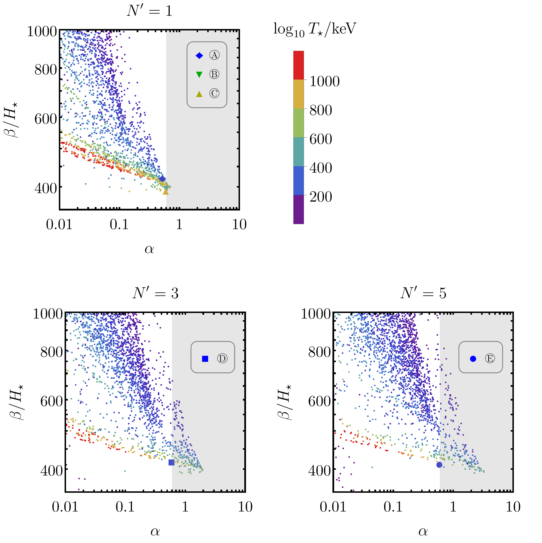
Figure 1: Scatter plot in the plane $\beta/H_{\star}$ versus $\alpha$ over the four parameters $v^{\prime}_{0}$, $M^{\prime}$, $\lambda^{\prime}$, $C$ and for the three values $N^{\prime}=1,3,5$ corresponding to the three panels. The shadowed region indicates that for $\alpha\gtrsim 0.6$ we do not have a reliable expression for the GW spectrum. In the first panel, for $N^{\prime}=1$, the diamond, lower and upper triangles indicate the three benchmark points in Table 1. The diamond in the first panel, the square in the second panel and the circle in the third panel indicate the three benchmark points in Table 2.

B.P.	$N^{\prime}$	$\lambda^{\prime}$	$v^{\prime}_{0}$ [keV]	$M^{\prime}$ [keV]	$C$ [keV]	$\alpha$	$\alpha_{\nu{\rm D}}$	$\kappa_{\nu{\rm D}}$	$\beta/H_{\star}$	$T_{\star}$ [keV]
A	1	$0.001$	$71.0$	$20.0$	$0.75$	$0.52$	$2.40$	$0.74$	$424.0$	$240.58$
B	1	$0.001$	$83.0$	$23.0$	$1.70$	$0.60$	$2.62$	$0.75$	$399.73$	$515.11$
C	1	$0.001$	$144.0$	$40.0$	$3.0$	$0.59$	$2.56$	$0.75$	$393.63$	$888.35$

Table 1: Benchmark points for GW signals from first order phase transition of $\phi^{\prime}$ for $N^{\prime}=1$.

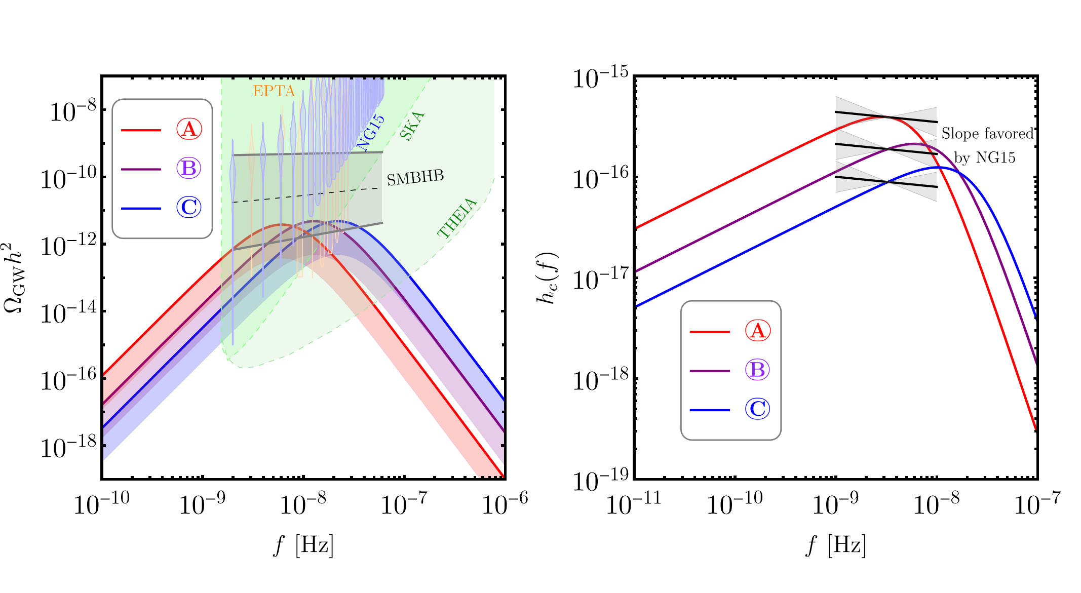
Figure 2: Left: GW spectrum at NANOGrav for $N^{\prime}=1$ and different $\alpha$. Right: Strain spectrum compared to best fit from NANOGrav 15-yr data. Benchmark points are given in Table 1.

B.P.	$N^{\prime}$	$\lambda^{\prime}$	$v^{\prime}_{0}$ [keV]	$M^{\prime}$ [keV]	$C$ [keV]	$\alpha$	$\alpha_{\nu{\rm D}}$	$\kappa_{\nu{\rm D}}$	$\beta/H_{\star}$	$T_{\star}$ [keV]
A	1	$0.001$	$71.0$	$20.0$	$0.75$	$0.52$	$2.40$	$0.74$	$424.0$	$240.58$
D	3	$0.001$	$129.0$	$29.0$	$1.20$	$0.59$	$2.092$	$0.71$	$420.93$	$262.61$
E	5	$0.0015$	$93.0$	$20.0$	$1.5$	$0.59$	$1.85$	$0.69$	$415.25$	$251.55$

Table 2: Benchmark points for phase transition of $\phi^{\prime}$ with $N^{\prime}=1,3,5$, respectively.

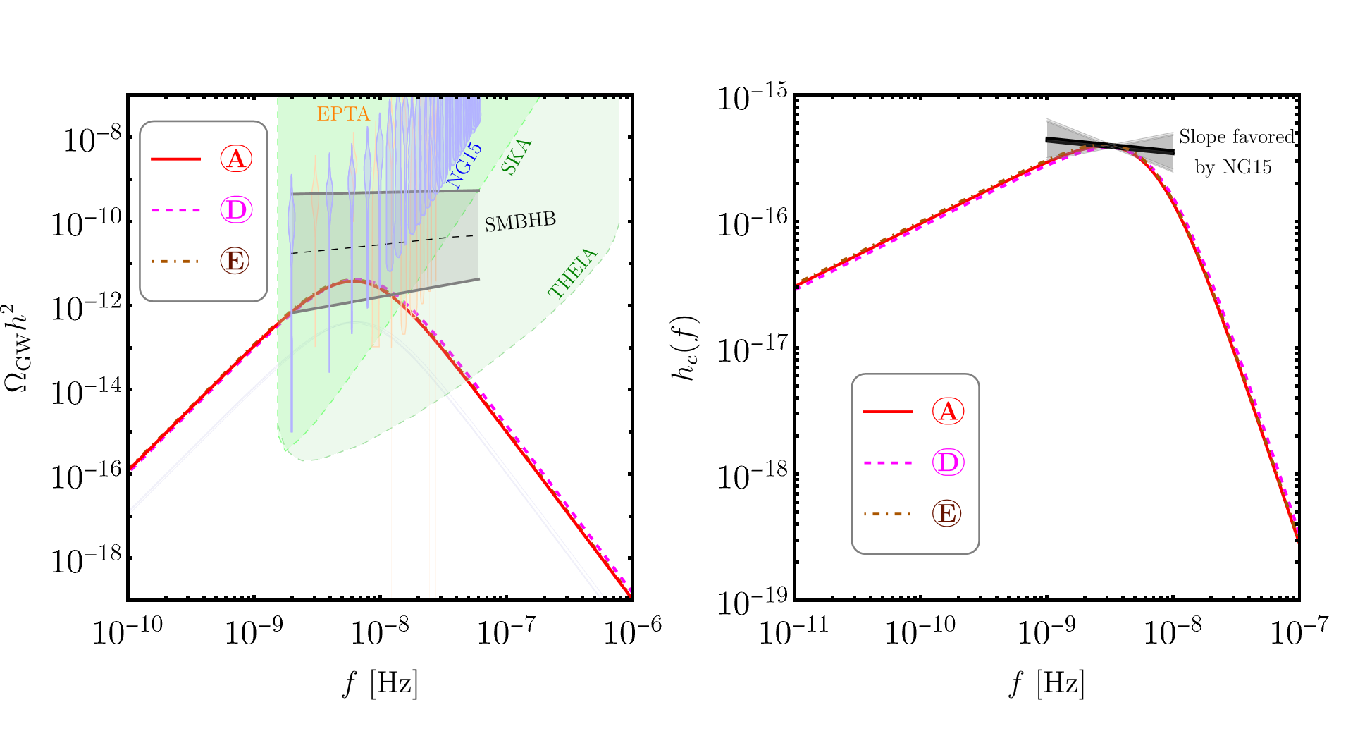
Figure 3: Left: GW spectrum at NANOGrav with different $N^{\prime}$. Right: Strain spectrum compared to best fit from NANOGrav 15-yr data. Benchmark points are given in Table 2.

The left panel of Fig. 2 shows three GW spectra, corresponding to the three benchmark points in Table 1, peaking in the frequency range probed by NANOGrav for $N^{\prime}=1$. The parameters $\alpha$ and $\beta/H_{\star}$ decrease and increase, respectively, from the benchmark point A to C, weakening the GW peak amplitude. In Fig. 3, we show two more benchmark points D and E, for $N^{\prime}=3$ and $N^{\prime}=5$ respectively, which have the same value of $\alpha$ as the benchmark point A, and slightly different $\beta/H_{\star}$. The resulting spectra is very similar, showing that the maximum GW signal that can be achieved in this model in the NANOGrav frequencies is somewhat independent of $N^{\prime}$ if $\alpha$ is upper bounded.

In the right panel of Figs. 2 and 3 we show the dimensionless strain $h_{c}(f)$ of the GW signals, given by

$$h_{c}(f)=\sqrt{\frac{2\mathcal{H}_{0}^{2}\Omega_{\rm GW}(f)}{2\pi^{2}f^{2}}},$$ (46)

where $\mathcal{H}_{0}\approx 68$ km/s/Mpc is today’s Hubble rate. We compare the results with the spectral slope $\beta={d\log h_{c}(f)}/{d\log f}$ modeling the NANOGrav strain spectrum with a simple power law of the form $h_{c}(f)=A_{\rm GW}(f/f_{\rm PTA})^{\beta}$. Expressing $\beta$ in terms of another parameter $\gamma_{\rm GW}=3-2\beta$, the $1\sigma$ fit to NANOGrav 15-yr data gives $\gamma_{\rm GW}\simeq 3.2\pm 0.6$ around $f\sim 1/(10\rm yr)$ [1]. This favorable range is shown with gray bands superimposed on our strain plot. We find that the spectral tilt of the phase transition signal is in tension in some range of the frequency band probed by NANOGrav.

5 Final remarks

Let us draw some final remarks on the results we obtained and how these can be further extended and improved.

• Our results are compatible with those presented in [64]. The differences can be mainly understood in terms of the different expression we are using to describe the GW spectrum from sound waves, the Eq. (30). This supersedes the expression used in [64] based on [65]. The suppression factor taking into account the shorter duration of the stage of GW production compared to the duration of the phase transition is somehow compensated by the fact that the new expression we are using is extended to higher values of $\alpha$. However, our description of bubble velocity in terms of Jouguet solutions should be clearly replaced by a more advanced one taking into account friction though we expect slight changes since the GW spectrum scales just linearly with $v_{\rm w}$. Another important difference is that compared to [65] the peak frequency is more than doubled and this explains why we obtain higher values of $T^{\prime}_{\star}\sim 100\,{\rm keV}$ for the peak value to be in the nHz range spanned by the NANOGrav signal. Also, notice that we have improved the calculation of the GW spectrum taking properly into account the different temperature of the dark sector and calculating the efficiency in terms of $\alpha_{\nu{\rm D}}$ rather than $\alpha$.

• The peak amplitude we find is at most $h^{2}\Omega_{\rm gw}(f)\sim 10^{-11}$ at the NANOGrav frequencies and cannot reproduce the whole NANOGrav signal. However, it can help the contribution from SMBHBs to improve the fit, one of the two options for the presence of new physics suggested by the NANOGrav collaboration analysis. This is certainly sufficient to make our results interesting, also considering that the model we studied is independently motivated by the cosmological tensions. Clearly, it would be interesting to perform a statistical analysis to find the best fit parameters in our model and to quantify the statistical significance.

• The possibility to have a higher peak amplitude, corresponding to $\xi\gg 1$, cannot be excluded but from current results from numerical simulations it seems unlikely. We just notice that increasing the value of $N^{\prime}$, values of $\alpha$ higher than 0.6 are possible and since firm predictions are missing for such strong first order transitions, one cannot exclude large enhancement coming, for example, from not yet understood contribution from turbulence. A specific account of the effect of small fluctuations within our model might also offer potentially a way to obtain $\xi\gg 1$.

• The values $T^{\prime}_{\star}\sim 100\,{\rm keV}$ that we found in our solutions that enter the NANOGrav frequency range, imply $\Delta N_{\nu}\simeq 0.4$ at the time of nucleosynthesis, for $N^{\prime}=1$. This is in marginal agreement with the constraint Eq. (17) from primordial deuterium measurements but it can be fully reconciled just simply assuming extra degrees of freedom in the dark sector ($\Delta g\neq 0$). On the other hand, such an amount of dark radiation at the time of nucleosynthesis might be even beneficial to solve a potential deuterium problem. Actually if such a deviation from SBBN should be confirmed, this would provide quite a strong support to the model. Moreover, as discussed, the same amount of dark radiation at recombination can ameliorate the cosmological tensions. In this respect a dedicated analysis within our model would be certainly desirable.

• One could think to explore a scenario with $T^{\prime}_{\star}\gg 1\,{\rm MeV}$, with a massive majoron $J^{\prime}$ quickly decaying before big bang nucleosynthesis thus avoiding all cosmological constraints [73, 74]. This would require an extension of the model introducing explicit symmetry breaking terms giving mass to $J^{\prime}$. However, it has been noticed that the introduction of these terms leading to a majoron mass larger than about 1 eV would actually jeopardise the occurrence of a first order phase transition [64]. For this reason this possibility does not seem viable, since the decay rate of extremely ultra-relativistic particles is strongly suppressed.

In conclusion the split majoron model is an appealing possibility to address part of the NANOGrav signal and the cosmoloical tensions, including, potentially, the deuterium problem. Moreover, it can have connections with other different phenomenologies. In any case it is certainly a clear example of how, with the evidence of a GW cosmological background from NANAOGrav, GWs have opened a new era in our quest of new physics. This should certainly alleviate the regret for the non-evidence of new physics at the LHC (at least so far).

Acknowledgments

We acknowledge financial support from the STFC Consolidated Grant ST/T000775/1. We also would like to thank David Weir for many useful discussions.

References

- [1] NANOGrav collaboration, The NANOGrav 15 yr Data Set: Evidence for a Gravitational-wave Background, Astrophys. J. Lett. 951 (2023) L8 [2306.16213].
- [2] NANOGrav collaboration, The NANOGrav 12.5 yr Data Set: Search for an Isotropic Stochastic Gravitational-wave Background, Astrophys. J. Lett. 905 (2020) L34 [2009.04496].
- [3] NANOGrav collaboration, Searching for Gravitational Waves from Cosmological Phase Transitions with the NANOGrav 12.5-Year Dataset, Phys. Rev. Lett. 127 (2021) 251302 [2104.13930].
- [4] NANOGrav collaboration, The NANOGrav 15 yr Data Set: Search for Signals from New Physics, Astrophys. J. Lett. 951 (2023) L11 [2306.16219].
- [5] R.w. Hellings and G.s. Downs, UPPER LIMITS ON THE ISOTROPIC GRAVITATIONAL RADIATION BACKGROUND FROM PULSAR TIMING ANALYSIS, Astrophys. J. Lett. 265 (1983) L39.
- [6] Z. Yi, Q. Gao, Y. Gong, Y. Wang and F. Zhang, The waveform of the scalar induced gravitational waves in light of Pulsar Timing Array data, 2307.02467.
- [7] Y.-T. Kuang, J.-Z. Zhou, Z. Chang, X. Zhang and Q.-H. Zhu, Primordial black holes from second order density perturbations as probes of the small-scale primordial power spectrum, 2307.02067.
- [8] D.G. Figueroa, M. Pieroni, A. Ricciardone and P. Simakachorn, Cosmological Background Interpretation of Pulsar Timing Array Data, 2307.02399.
- [9] C. Unal, A. Papageorgiou and I. Obata, Axion-Gauge Dynamics During Inflation as the Origin of Pulsar Timing Array Signals and Primordial Black Holes, 2307.02322.
- [10] K.T. Abe and Y. Tada, Translating nano-Hertz gravitational wave background into primordial perturbations taking account of the cosmological QCD phase transition, 2307.01653.
- [11] G. Cacciapaglia, D.Y. Cheong, A. Deandrea, W. Isnard and S.C. Park, Composite Hybrid Inflation: Dilaton and Waterfall Pions, 2307.01852.
- [12] L.A. Anchordoqui, I. Antoniadis and D. Lust, Fuzzy Dark Matter, the Dark Dimension, and the Pulsar Timing Array Signal, 2307.01100.
- [13] S.-P. Li and K.-P. Xie, Collider test of nano-Hertz gravitational waves from pulsar timing arrays, Phys. Rev. D 108 (2023) 055018 [2307.01086].
- [14] Y. Xiao, J.M. Yang and Y. Zhang, Implications of Nano-Hertz Gravitational Waves on Electroweak Phase Transition in the Singlet Dark Matter Model, 2307.01072.
- [15] B.-Q. Lu and C.-W. Chiang, Nano-Hertz stochastic gravitational wave background from domain wall annihilation, 2307.00746.
- [16] C. Zhang, N. Dai, Q. Gao, Y. Gong, T. Jiang and X. Lu, Detecting new fundamental fields with Pulsar Timing Arrays, 2307.01093.
- [17] R.A. Konoplya and A. Zhidenko, Asymptotic tails of massive gravitons in light of pulsar timing array observations, 2307.01110.
- [18] D. Chowdhury, G. Tasinato and I. Zavala, Dark energy, D-branes, and Pulsar Timing Arrays, 2307.01188.
- [19] X. Niu and M.H. Rahat, NANOGrav signal from axion inflation, 2307.01192.
- [20] L. Liu, Z.-C. Chen and Q.-G. Huang, Implications for the non-Gaussianity of curvature perturbation from pulsar timing arrays, 2307.01102.
- [21] J.R. Westernacher-Schneider, J. Zrake, A. MacFadyen and Z. Haiman, Characteristic signatures of accreting binary black holes produced by eccentric minidisks, 2307.01154.
- [22] Y. Gouttenoire, S. Trifinopoulos, G. Valogiannis and M. Vanvlasselaer, Scrutinizing the Primordial Black Holes Interpretation of PTA Gravitational Waves and JWST Early Galaxies, 2307.01457.
- [23] T. Ghosh, A. Ghoshal, H.-K. Guo, F. Hajkarim, S.F. King, K. Sinha et al., Did we hear the sound of the Universe boiling? Analysis using the full fluid velocity profiles and NANOGrav 15-year data, 2307.02259.
- [24] S. Datta, Inflationary gravitational waves, pulsar timing data and low-scale-leptogenesis, 2307.00646.
- [25] D. Borah, S. Jyoti Das and R. Samanta, Inflationary origin of gravitational waves with \textitMiracle-less WIMP dark matter in the light of recent PTA results, 2307.00537.
- [26] B. Barman, D. Borah, S. Jyoti Das and I. Saha, Scale of Dirac leptogenesis and left-right symmetry in the light of recent PTA results, 2307.00656.
- [27] Y.-C. Bi, Y.-M. Wu, Z.-C. Chen and Q.-G. Huang, Implications for the Supermassive Black Hole Binaries from the NANOGrav 15-year Data Set, 2307.00722.
- [28] S. Wang, Z.-C. Zhao, J.-P. Li and Q.-H. Zhu, Exploring the Implications of 2023 Pulsar Timing Array Datasets for Scalar-Induced Gravitational Waves and Primordial Black Holes, 2307.00572.
- [29] T. Broadhurst, C. Chen, T. Liu and K.-F. Zheng, Binary Supermassive Black Holes Orbiting Dark Matter Solitons: From the Dual AGN in UGC4211 to NanoHertz Gravitational Waves, 2306.17821.
- [30] S. Jiang, A. Yang, J. Ma and F.P. Huang, Implication of nano-Hertz stochastic gravitational wave on dynamical dark matter through a first-order phase transition, 2306.17827.
- [31] A. Eichhorn, R.R. Lino dos Santos and J.a.L. Miqueleto, From quantum gravity to gravitational waves through cosmic strings, 2306.17718.
- [32] H.-L. Huang, Y. Cai, J.-Q. Jiang, J. Zhang and Y.-S. Piao, Supermassive primordial black holes in multiverse: for nano-Hertz gravitational wave and high-redshift JWST galaxies, 2306.17577.
- [33] Y. Gouttenoire and E. Vitagliano, Domain wall interpretation of the PTA signal confronting black hole overproduction, 2306.17841.
- [34] Y.-F. Cai, X.-C. He, X. Ma, S.-F. Yan and G.-W. Yuan, Limits on scalar-induced gravitational waves from the stochastic background by pulsar timing array observations, 2306.17822.
- [35] K. Inomata, K. Kohri and T. Terada, The Detected Stochastic Gravitational Waves and Subsolar-Mass Primordial Black Holes, 2306.17834.
- [36] G. Lazarides, R. Maji and Q. Shafi, Superheavy quasi-stable strings and walls bounded by strings in the light of NANOGrav 15 year data, 2306.17788.
- [37] P.F. Depta, K. Schmidt-Hoberg, P. Schwaller and C. Tasillo, Do pulsar timing arrays observe merging primordial black holes?, 2306.17836.
- [38] S. Blasi, A. Mariotti, A. Rase and A. Sevrin, Axionic domain walls at Pulsar Timing Arrays: QCD bias and particle friction, 2306.17830.
- [39] L. Bian, S. Ge, J. Shu, B. Wang, X.-Y. Yang and J. Zong, Gravitational wave sources for Pulsar Timing Arrays, 2307.02376.
- [40] G. Franciolini, D. Racco and F. Rompineve, Footprints of the QCD Crossover on Cosmological Gravitational Waves at Pulsar Timing Arrays, 2306.17136.
- [41] Z.-Q. Shen, G.-W. Yuan, Y.-Y. Wang and Y.-Z. Wang, Dark Matter Spike surrounding Supermassive Black Holes Binary and the nanohertz Stochastic Gravitational Wave Background, 2306.17143.
- [42] G. Lambiase, L. Mastrototaro and L. Visinelli, Astrophysical neutrino oscillations after pulsar timing array analyses, 2306.16977.
- [43] C. Han, K.-P. Xie, J.M. Yang and M. Zhang, Self-interacting dark matter implied by nano-Hertz gravitational waves, 2306.16966.
- [44] S.-Y. Guo, M. Khlopov, X. Liu, L. Wu, Y. Wu and B. Zhu, Footprints of Axion-Like Particle in Pulsar Timing Array Data and JWST Observations, 2306.17022.
- [45] Z. Wang, L. Lei, H. Jiao, L. Feng and Y.-Z. Fan, The nanohertz stochastic gravitational-wave background from cosmic string Loops and the abundant high redshift massive galaxies, 2306.17150.
- [46] J. Ellis, M. Lewicki, C. Lin and V. Vaskonen, Cosmic Superstrings Revisited in Light of NANOGrav 15-Year Data, 2306.17147.
- [47] S. Vagnozzi, Inflationary interpretation of the stochastic gravitational wave background signal detected by pulsar timing array experiments, JHEAp 39 (2023) 81 [2306.16912].
- [48] K. Fujikura, S. Girmohanta, Y. Nakai and M. Suzuki, NANOGrav Signal from a Dark Conformal Phase Transition, 2306.17086.
- [49] N. Kitajima, J. Lee, K. Murai, F. Takahashi and W. Yin, Nanohertz Gravitational Waves from Axion Domain Walls Coupled to QCD, 2306.17146.
- [50] G. Franciolini, A. Iovino, Junior., V. Vaskonen and H. Veermae, The recent gravitational wave observation by pulsar timing arrays and primordial black holes: the importance of non-gaussianities, 2306.17149.
- [51] E. Megias, G. Nardini and M. Quiros, Pulsar Timing Array Stochastic Background from light Kaluza-Klein resonances, 2306.17071.
- [52] J. Ellis, M. Fairbairn, G. Hütsi, J. Raidal, J. Urrutia, V. Vaskonen et al., Gravitational Waves from SMBH Binaries in Light of the NANOGrav 15-Year Data, 2306.17021.
- [53] Y. Bai, T.-K. Chen and M. Korwar, QCD-Collapsed Domain Walls: QCD Phase Transition and Gravitational Wave Spectroscopy, 2306.17160.
- [54] J. Yang, N. Xie and F.P. Huang, Implication of nano-Hertz stochastic gravitational wave background on ultralight axion particles, 2306.17113.
- [55] A. Ghoshal and A. Strumia, Probing the Dark Matter density with gravitational waves from super-massive binary black holes, 2306.17158.
- [56] H. Deng, B. Bécsy, X. Siemens, N.J. Cornish and D.R. Madison, Searching for gravitational wave burst in PTA data with piecewise linear functions, 2306.17130.
- [57] P. Athron, A. Fowlie, C.-T. Lu, L. Morris, L. Wu, Y. Wu et al., Can supercooled phase transitions explain the gravitational wave background observed by pulsar timing arrays?, 2306.17239.
- [58] A. Addazi, Y.-F. Cai, A. Marciano and L. Visinelli, Have pulsar timing array methods detected a cosmological phase transition?, 2306.17205.
- [59] V.K. Oikonomou, Flat energy spectrum of primordial gravitational waves versus peaks and the NANOGrav 2023 observation, Phys. Rev. D 108 (2023) 043516 [2306.17351].
- [60] N. Kitajima and K. Nakayama, Nanohertz gravitational waves from cosmic strings and dark photon dark matter, 2306.17390.
- [61] A. Mitridate, D. Wright, R. von Eckardstein, T. Schröder, J. Nay, K. Olum et al., PTArcade, 2306.16377.
- [62] S.F. King, D. Marfatia and M.H. Rahat, Towards distinguishing Dirac from Majorana neutrino mass with gravitational waves, 2306.05389.
- [63] J. Liu, Distinguishing nanohertz gravitational wave sources through the observations of ultracompact minihalos, 2305.15100.
- [64] P. Di Bari, D. Marfatia and Y.-L. Zhou, Gravitational waves from first-order phase transitions in Majoron models of neutrino mass, JHEP 10 (2021) 193 [2106.00025].
- [65] C. Caprini et al., Science with the space-based interferometer eLISA. II: Gravitational waves from cosmological phase transitions, JCAP 04 (2016) 001 [1512.06239].
- [66] D. Cutting, M. Hindmarsh and D.J. Weir, Vorticity, kinetic energy, and suppressed gravitational wave production in strong first order phase transitions, Phys. Rev. Lett. 125 (2020) 021302 [1906.00480].
- [67] P. Di Bari, S.F. King and M.H. Rahat, Gravitational waves from phase transitions and cosmic strings in neutrino mass models with multiple Majorons, 2306.04680.
- [68] Y. Chikashige, R.N. Mohapatra and R.D. Peccei, Are There Real Goldstone Bosons Associated with Broken Lepton Number?, Phys. Lett. B 98 (1981) 265.
- [69] P. Di Bari, Cosmology and the early Universe, Series in Astronomy and Astrophysics, CRC Press (5, 2018).
- [70] B.D. Fields, K.A. Olive, T.-H. Yeh and C. Young, Big-Bang Nucleosynthesis after Planck, JCAP 03 (2020) 010 [1912.01132].
- [71] O. Pisanti, G. Mangano, G. Miele and P. Mazzella, Primordial Deuterium after LUNA: concordances and error budget, JCAP 04 (2021) 020 [2011.11537].
- [72] Planck collaboration, Planck 2018 results. VI. Cosmological parameters, Astron. Astrophys. 641 (2020) A6 [1807.06209].
- [73] M. Fairbairn, E. Hardy and A. Wickens, Hearing without seeing: gravitational waves from hot and cold hidden sectors, JHEP 07 (2019) 044 [1901.11038].
- [74] T. Bringmann, P.F. Depta, T. Konstandin, K. Schmidt-Hoberg and C. Tasillo, Does NANOGrav observe a dark sector phase transition?, 2306.09411.
- [75] Z. Chacko, L.J. Hall, T. Okui and S.J. Oliver, CMB signals of neutrino mass generation, Phys. Rev. D 70 (2004) 085008 [hep-ph/0312267].
- [76] M. Escudero and S.J. Witte, A CMB search for the neutrino mass mechanism and its relation to the Hubble tension, Eur. Phys. J. C 80 (2020) 294 [1909.04044].
- [77] M. Escudero and S.J. Witte, The hubble tension as a hint of leptogenesis and neutrino mass generation, Eur. Phys. J. C 81 (2021) 515 [2103.03249].
- [78] M. Cielo, M. Escudero, G. Mangano and O. Pisanti, Neff in the Standard Model at NLO is 3.043, 2306.05460.
- [79] N. Blinov and G. Marques-Tavares, Interacting radiation after Planck and its implications for the Hubble Tension, JCAP 09 (2020) 029 [2003.08387].
- [80] S. Sandner, M. Escudero and S.J. Witte, Precision CMB constraints on eV-scale bosons coupled to neutrinos, Eur. Phys. J. C 83 (2023) 709 [2305.01692].
- [81] R.J. Cooke, M. Pettini and C.C. Steidel, One Percent Determination of the Primordial Deuterium Abundance, Astrophys. J. 855 (2018) 102 [1710.11129].
- [82] C. Pitrou, A. Coc, J.-P. Uzan and E. Vangioni, A new tension in the cosmological model from primordial deuterium?, Mon. Not. Roy. Astron. Soc. 502 (2021) 2474 [2011.11320].
- [83] P. Di Bari, Update on neutrino mixing in the early universe, Phys. Rev. D 65 (2002) 043509 [hep-ph/0108182].
- [84] C. Pitrou, A. Coc, J.-P. Uzan and E. Vangioni, Resolving conclusions about the early Universe requires accurate nuclear measurements, Nature Rev. Phys. 3 (2021) 231 [2104.11148].
- [85] M. Hindmarsh, S.J. Huber, K. Rummukainen and D.J. Weir, Shape of the acoustic gravitational wave power spectrum from a first order phase transition, Phys. Rev. D 96 (2017) 103520 [1704.05871].
- [86] D.J. Weir, Gravitational waves from a first order electroweak phase transition: a brief review, Phil. Trans. Roy. Soc. Lond. A 376 (2018) 20170126 [1705.01783].
- [87] P.J. Steinhardt, Relativistic Detonation Waves and Bubble Growth in False Vacuum Decay, Phys. Rev. D 25 (1982) 2074.
- [88] J.R. Espinosa, T. Konstandin, J.M. No and G. Servant, Energy Budget of Cosmological First-order Phase Transitions, JCAP 06 (2010) 028 [1004.4187].
- [89] J. Ellis, M. Lewicki and J.M. No, On the Maximal Strength of a First-Order Electroweak Phase Transition and its Gravitational Wave Signal, JCAP 04 (2019) 003 [1809.08242].
- [90] H.-K. Guo, K. Sinha, D. Vagie and G. White, Phase Transitions in an Expanding Universe: Stochastic Gravitational Waves in Standard and Non-Standard Histories, JCAP 01 (2021) 001 [2007.08537].
- [91] M. Hindmarsh, S.J. Huber, K. Rummukainen and D.J. Weir, Numerical simulations of acoustically generated gravitational waves at a first order phase transition, Phys. Rev. D 92 (2015) 123009 [1504.03291].
- [92] M. Kamionkowski, A. Kosowsky and M.S. Turner, Gravitational radiation from first order phase transitions, Phys. Rev. D 49 (1994) 2837 [astro-ph/9310044].
- [93] P. Auclair, C. Caprini, D. Cutting, M. Hindmarsh, K. Rummukainen, D.A. Steer et al., Generation of gravitational waves from freely decaying turbulence, JCAP 09 (2022) 029 [2205.02588].
- [94] M.A. Ajmi and M. Hindmarsh, Thermal suppression of bubble nucleation at first-order phase transitions in the early Universe, Phys. Rev. D 106 (2022) 023505 [2205.04097].
- [95] R. Jinno, T. Konstandin, H. Rubira and J. van de Vis, Effect of density fluctuations on gravitational wave production in first-order phase transitions, JCAP 12 (2021) 019 [2108.11947].