: Improving Visual Representations by Circumventing Text Feature Learning

Abstract

Large web-sourced multimodal datasets have powered a slew of new methods for learning general-purpose visual representations, advancing the state of the art in computer vision and revolutionizing zero- and few-shot recognition. One crucial decision facing practitioners is how, if at all, to curate these ever-larger datasets. For example, the creators of the LAION-5B dataset chose to retain only image-caption pairs whose CLIP similarity score exceeded a designated threshold. In this paper, we propose a new state-of-the-art data filtering approach motivated by our observation that nearly $40\%$ of LAION’s images contain text that overlaps significantly with the caption. Intuitively, such data could be wasteful as it incentivizes models to perform optical character recognition rather than learning visual features. However, naively removing all such data could also be wasteful, as it throws away images that contain visual features (in addition to overlapping text). Our simple and scalable approach, (Text Masking and Re-Scoring), filters out only those pairs where the text dominates the remaining visual features—by first masking out the text and then filtering out those with a low CLIP similarity score of the masked image. Experimentally, outperforms the top-ranked method on the “medium scale” of DataComp (a data filtering benchmark) by a margin of $6.5\%$ on ImageNet and $4.7\%$ on VTAB. Additionally, our systematic evaluation on various data pool sizes from 2M to 64M shows that the accuracy gains enjoyed by linearly increase as data and compute are scaled exponentially. Code is available at https://github.com/locuslab/T-MARS.

1 Introduction

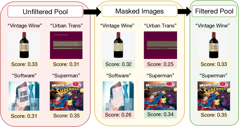
(a)

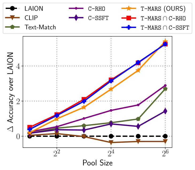
(b)

Figure 1: (a) Given an unfiltered pool of image-caption pairs, first masks the text present in each image, and calculates the similarity between the masked image and the corresponding caption, retaining only those with high similarity scores. (b) Scaling curves depicting a linear increase accuracy as data is increased exponentially when training ViT-B-32 models on filtered data versus training on the LAION dataset. The training compute is scaled proportionally with the pool size.

The paradigm of machine learning has shifted from training on carefully crafted labeled datasets to training on large crawls of the web [1]. Vision-language models like CLIP [40] and BASIC [38] trained on web-scale datasets have demonstrated exceptional zero-shot performance across a wide range of vision tasks, and the representations that they learn have become the de-facto standard across a variety of vision domains. Recently, the OpenCLIP [23] effort has aimed to independently reproduce the performance of the original CLIP model through the curation of a similarly sized LAION-400M [45] dataset. However, they are still unable to match the performance of CLIP, suggesting that data curation could play an important role even at web-scale. Most recently, the launch of ‘DataComp’ [14], a data filtering competition at various web-scale, has further streamlined efforts in this field.

Data curation at web scale raises unique challenges compared to the standard classification regime. In web-scale datasets, we typically make only a single (or few) pass(es) over each training example [21], as it is often beneficial to see a fresh batch of data from the virtually unbounded web-scale data. However, prior data pruning approaches that characterize the hardness of individual data points [36, 34] were proposed for, and evaluated on models trained to convergence in the standard setting. More importantly, any data curation method has to be adaptable to the multimodal contrastive learning setting, and scalable to billions of samples, rendering several prior methods simply infeasible [48].

In this work, we propose a new state-of-the-art data filtering approach for large-scale image-text datasets. We start by looking at how the image and text modalities interact in these datasets. We find that around $40\%$ of examples in the LAION dataset have text in the image—for example book covers (Figure 1). This text is often the only element correlated with the caption, necessitating that the contrastive learning objective learns to solve an “optical character recognition” (OCR) task. This is wasteful if we were only interested in purely visual features which are relevant for downstream vision tasks. Conversely, however, naively removing all such images that contain text (e.g., similar to Radenovic et al. [39]), discards a substantial portion of images that contain both visual and well as text features. For example, the “vintage wine” image from Figure 1 provides useful visual cues about what a bottle of wine looks like, despite containing overlapping text with caption.

Our simple and scalable method, Text-Masking and Re-Scoring (T-MARS) filters out examples where the text feature dominate the visual features in their contribution to matching to the corresponding caption. Specifically, we first mask the text inside images and then calculate the cosine similarity score of the masked image embedding with that of the caption. Finally, we filter out images with a low similarity score (see Figure 1(a)). We establish as a state-of-the-art data filtering technique, by extensively evaluating on 6 different subsets of LAION at exponentially increasing scales (2M to 64M), where outperforms the most competitive baseline by as much as $3.7\%$ on ImageNet zeroshot accuracy. Similarly, on a recently released DataComp [14] benchmark, outperforms the top of the “medium scale” leaderboard by more than $6.5\%$. Notably, training on a pool with filtering, can even outperform training on a CLIP score-filtered pool, seeing only half the training samples at 50% total compute. We additionally present scaling experiments for our approach: through experiments on pool sizes ranging from 2M to 64M, we showcase a surprising linear increase in accuracy gains as the pool size is scaled exponentially (Figure 1). Our scaling trends highlight that good-quality data filtering holds even more significance at larger scales.

To develop a fundamental understanding behind our gains, we plot utility curves for various image types (based on the features present) by modifying the ImageNet-Captions dataset [10]. Our experiments show that (a) images with both visual and text features have nearly the same utility as those with just visual features; and (b) images with only text have the same negative utility as mislabeled samples (§ 7), hurting downstream performance. Finally, we also introduce and benchmark two competitive data filtering baselines, C-RHO and C-SSFT, by drawing insights from the long line of work in the supervised classification regime on hard example mining (§ 5.2). These baselines themselves perform better than the widely used CLIP score based filtering and notably can boost performance when we take an intersection of the data retained by and the proposed baselines.

With the ML community focused on scaling up dataset sizes, our experiments most notably show that pruning off ‘bad data’ can have $3\times$ more utility than adding more ‘good’ samples to the dataset.

2 Related Work

Data Curation for Web-Scale Datasets

Following the curation of the LAION-5B [45, 46] datasets, there has been a growing interest in exploring improved strategies for selecting subsets of the common crawl that help learn better visual representations. Recently, Radenovic et al. [39] suggested using a mixture of three metrics, namely, complexity, action, and text-match (does the associated caption describe an action that contains a complex object relationship? does the text in the image match with a part of the caption?) Retaining examples based on complexity and action metrics are seen to hurt zero-shot performance, whereas filtering out examples with text-match helps. This works required text-recognition to match the text with caption, which requires an order of magnitude more compute than text detection required for our proposed masking approach. Abbas et al. [2] noted that web-scale datasets have a large number of near and exact duplicates, and removed such duplicates to speed up training, similar to such efforts in datasets for language modeling  [41, 30]. Finally, given metadata for tasks of interest, e.g., class names for ImageNet classes, and a large pool of image-text pairs, CiT [52] was proposed to select relevant training data from the pool by measuring the similarity of their text embeddings and embeddings of the metadata. However, this method does not allow learning general-purpose vision representations. Most recently, DataComp [14] was introduced as a benchmark challenge for subset selection from common crawl. Among various baselines established by them, the authors found that filtering based on CLIP score is the best-performing approach.

Hard Example Mining in Supervised Classification

Coreset selection [11, 3, 16] and outlier removal [43, 25, 54] has been extensively explored in the literature to select a subset of data that achieves a similar or better performance. However, these approaches are quite computationally expensive and hard to extend to web-scale. Other lines of work have focused on finding and prioritizing training on hard examples, which are filtered using memorization and influence scores [13, 12, 26], or based on the learning dynamics of different samples  [6, 35, 47, 28, 5]. More recent works studying realistic dataset settings such as those with noisy examples discovered that prioritizing so-called ‘hard’ examples may be a suboptimal approach because it also incentivizes prioritizing the training on mislabeled examples. Mindermann et al. [36] proposed the RHO (robust hold-out) loss and Maini et al. [34] proposed the SSFT (second-split forgetting time) towards identifying mislabeled examples. In Section 5.2, we discuss our adaptations of these ideas in the contrastive loss setting.

Vision-language pre-training

Image-language contrastive pre-training on web-scale datasets has gathered significant interest from the research community, because of the impressive zero-shot performance on the downstream tasks [40, 23, 7, 24, 31, 32, 38, 50, 53, 15, 37, 33]. CLIP [40] released the first large-scale vision-language model, obtaining around $75\%$ zero-shot accuracy on ImageNet. BASIC [38] scaled up the model size, compute, and data to further drive up performance gains. In this work, we aim to improve the zero-shot performance by only modifying the subset of data we train on.

Neural Scaling Laws

Recent works have shown a power law relation of test error with model size, compute and training samples in the standard classification regime [20, 56, 19]. Others have explored neural scaling laws for large language model and try to answer how the model size and training tokens should be scaled with compute [21, 9, 27]. Recently, Sorscher et al. [48] explored the use of data curation in the classification settings to achieve accuracies beyond those predicted by these power laws. In this work, we consider data curation in the multimodal vision-language model training regime.

3 Preliminaries

Task: Consider a pretraining image-caption dataset $\mathcal{S}=\{({i},{t})\}^{n}$, used to train CLIP [40] style models using contrastive learning. Given a fixed computation budget (number of training iterations), our goal is to find a subset of the dataset $\hat{\mathcal{S}}\subset\mathcal{S}$, such that models trained on $\hat{\mathcal{S}}$ have higher zero-shot accuracy on downstream tasks (such as image classification) than those trained on $\mathcal{S}$.

Zeroshot Accuracy: Given $k$ class names $\{c_{1},\dots c_{k}\}$ for an image-classification task, we construct corresponding text descriptions $\{{t}_{1},\ldots{t}_{k}\}$ (eg. ‘Photo of a $c_{i}$’). Then, the zero-shot prediction for image ${i}$ is given by $\operatorname*{arg\,max}_{j}g({t}_{j})^{\top}f({i})$, where $f,g$ are the image and language encoders.

CLIP similarity score: For a given image-caption pair $({i},{t})$, the CLIP similarity score refers to the cosine similarity between the embeddings of the image and the caption, i.e., $f({i})^{\top}g({t})/{\|f({i})\|_{2}\|g({t})\|_{2}}$.

4 What constitutes the LAION dataset? A pilot study

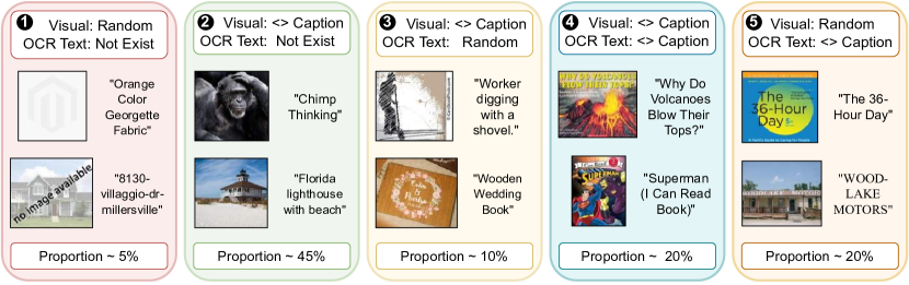
Figure 2: A representation of the various types of examples in the LAION dataset. ‘<>’ reads as ‘is correlated with’. A significant proportion of examples have some form of text overlayed on the image.

An analysis of image-caption pairs in web-crawled datasets is crucial to understanding the features in the image that models may utilize to align image and caption embeddings. To address this, we perform a small pilot study on 500 image-caption pairs from the LAION dataset. Our analysis yields an interesting observation—approximately 40% of the images possess “text” features (i.e. text written on the image) that correlate with the caption. In fact, nearly 20% times such text features constitute the sole element in the image that is correlated with the caption (eg. Book Covers). However, at the same time, a substantial fraction of these images exhibit both text features and general visual cues. For example, an image of a wine bottle with the word "vintage" written on it, accompanied by the caption "vintage wine". These observations lead us to classify the data into five categories based on the correlation between image features (text or visual) and the caption (See Figure 2):

1. Un-correlated Image and Caption $(\mathcal{S}_{r};\;3.7\%$): These pairs are essentially mislabeled, with no correlation between the image and caption. These typically exist due to missing image links.

2. Correlated Visual Feature and Caption $(\mathcal{S}_{i};\;46.7\%$): This is the most common category, where the image accurately corresponds to the caption and contains no text.

3. Correlated Visual Feature and Caption, Random OCR Text $(\mathcal{S}_{irt};\;9.8\%$): Some images include unrelated random text, such as website names. The model would typically disregard such text as it does not contribute to aligning the embedding with the caption.

4. Both Visual Feature and OCR Text correlated with Caption $(\mathcal{S}_{it};\;19.1\%$): These images contain both text and visual features that are correlated with the caption. For instance, in category 4 of Figure 2, the image of Superman includes the visual representation of Superman as well as the text "I can read: Superman," which aligns with the caption. It remains unclear whether the model would prioritize text or visual features in such cases.

5. Correlated OCR Text and Caption $(\mathcal{S}_{t};\;20.7\%$): These images lack visual information and solely consist of text heavily correlated with the caption. Many book covers constitute this type. These images would simply incentivize the model to learn the problem of optical character recognition.

The above classification is based on our manual judgement of the correlation between the various features and caption. Given an image with text features (category 3 to 5), we ascertain the text as correlated with the caption if they have overlapping words or convey similar meaning. Similarly, we ascertain visual features as correlated with the caption if the caption is a non-vague description of the visual feature. In the next section, we use these findings to motivate and propose our data curation approach, T-MARS. Note that our experiments on text detection in § 6.3 further confirm that the estimated proportions based on our pilot study hold even at 64M scale LAION data subsets.

5 Method

Our pilot study in the § 4 revealed that a significant portion of the dataset consists of images for which text is the sole feature associated with the caption. Intuitively, these images encourage the model to solve optical character recognition in order to align the image and caption representations. Considering our downstream goal of learning better visual representations, it is natural to filter out such images. However, simply removing images that contain text matching the caption, as suggested by previous work [39], may not be optimal. This is because our pilot study also highlights the presence of images that possess both text and visual features correlated with the caption.

5.1 : Text-Masking and Re-Scoring

Algorithm 1

  Input: Dataset $\mathcal{S}=\{{i},{t}\}^{n}$, score function $\ell$, image masking function $m$

  Output: Filtered Pool $\tilde{\mathcal{S}}$

  // Step 1: Text-Masking

  for $k=0\dots n-1$ do

     $\tilde{{i}}_{k}=m({{i}_{k}})$

  end for

  // Step 2: Re-Scoring

  for $k=0\dots n-1$ do

     $s_{k}=\ell(\tilde{{i}}_{k},{t}_{k})$

  end for

  $\alpha=\text{Median }(\{s_{k}\}_{k=1}^{n})$

  return $\tilde{\mathcal{S}}=\{({i}_{k},{t}_{k})\;|\;s_{k}\geq\alpha\}$

Based on the above hypothesis, we propose a simple and scalable approach, called , which focuses on evaluating the similarity of only the visual features in an image with its corresponding caption. involves masking out the text in the images and then calculating the similarity score between the masked image and the caption using a pretrained CLIP model. By filtering out images with low masked similarity scores, we can effectively curate the dataset. The main steps of our proposed approach are:

1. Text Detection: We apply a text detection algorithm (FAST [8]) that identifies the bounding boxes of text regions in the image (Figure 1). Notably, text detection focuses on localizing text positions in the image rather than recognizing or reading the text itself. This key distinction allows our approach to be an order of magnitude more scalable compared to text recognition-based filtering methods [39].

1. Text Masking: We mask the text regions by replacing them with the average color of the surrounding pixels within the respective bounding box.

2. Re-Scoring and Filtering: Using a pre-trained CLIP model, we calculate the cosine similarity between the masked image and the original caption. Finally, we simply filter out 50 percent of the datapoints that have the lowest similarity scores between the masked image and the caption.

We filter out $50\%$ of the pool to simplify the design choices. Note that we use the corresponding original images for training on the filtered subset, and not the masked images themselves. Algorithm Box 1 provides a detailed description of .

We first highlight the empirical effectiveness of in Section 6.3. Later, in Section 7—(1) We show that indeed works as intended, filtering out the images with only text features, while retaining those with both visual and text features, and (2) Through a series of toy experiments, we verify our initial hypothesis that features present in the image determine their utility. We show that images with text only features indeed hurt, surprisingly to the extent of mislabeled images.

5.2 Contributed Baselines

C-SSFT

Maini et al. [34] proposed the SSFT (Second-Split Forgetting Time) to identify mislabeled examples in a dataset by fine-tuning a converged model on validation data, and observing which examples change their predicted label the earliest. Given the absence of a converged model in webscale learning, we use a pretrained model from OpenCLIP [23] and finetune for $n=5$ epochs on the Conceptual-Captions dataset with a learning rate of $1e^{-5}$. We then calculate the average cosine similarity for all examples during the fine-tuning (forgetting) phase and rank examples based on the average similarity score, retaining only the highest-scoring ones.

C-RHO

Mindermann et al. [36] proposed RHO loss to prioritize the training on examples that are learnable, worth learning, and not yet learned. In the classification setup, at every epoch, the authors calculate the difference between the model’s training loss on a given data point and a validation model’s loss on the same data point. Examples with low validation loss, but high training loss are prioritized. In the regime of webscale datasets, the ordering of examples in an active learning fashion at every epoch is infeasible. Rather, we propose C-RHO to adapt to such a setting. (1) Rather than using the training loss, we utilize the model’s image-caption similarity score (because the contrastive loss is batch-specific and highly variable); (2) We train our model for one epoch on the entire dataset to calculate the training loss and use a model trained on CC3M dataset as the validation model. Then, we calculate the difference in training and validation similarity scores to rerank the examples and only keep the top 50% of examples for training afresh. $\texttt{C-RHO}({i},{t},\mathcal{S})=\mathcal{M}_{CC3}^{32}({i},{t})-\mathcal{M}_{\mathcal{S}}^{1}({i},{t}),$ where $\texttt{C-RHO}({i},{t},\mathcal{S})$ is the score for an image-caption pair (${i},{t}$) in a dataset $\mathcal{S}$, and $\mathcal{M}_{\mathcal{S}}^{n}$ is the similarity score based on a model trained for $n$ epochs on dataset $\mathcal{S}$.

5.3 Existing Baselines

We additionally compare against the following web-scale filtering approaches from the literature.

LAION filtering

The initial curation of the LAION-400M [45] and LAION-5B [46] datasets was based on filtering out image-caption subsets of the common crawl that had a similarity score of less than 0.281 as evaluated using OpenAI’s CLIP ViT-B/32 model [40]. Additionally, LAION-400M subset used language filtering to only keep captions that were written in English.

CLIP Score

We also investigate the use of stronger CLIP score thresholding by retaining image-caption pairs with high similarity to further reduce the size of the training pool by 50%. This would mean training multiple epochs on high CLIP-scored data, as opposed to a single epoch on all the data.

Text Match

Recently, Radenovic et al. [39] proposed removing all the images which contain text overlapping with the caption (5 continuous characters) to ensure that model only focuses on visual features in the dataset. We skip the caption complexity and caption action filtering part, since it is shown to have a negative impact on accuracy in the original paper. Importantly, note that Text Match is $10\times$ more costly than just text masking, and the quality of text recognition in web images is so low that state-of-art recognition algorithms are unable to identify all text in the image correctly. On the other hand, text masking used in our work only requires detection, which is fast and accurate. More discussion on the same is available in Appendix B.

6 Experiments

We evaluate various baselines (including those laid by this work) as well as our proposed approach across 7 different data pools ranging from 2 million to 128 million. Our results showcase a linear scaling trend in the zero-shot accuracy gains over no data curation, highlighting the importance of incorporating data curation in practice as the data and compute are scaled.

Table 1: Zero-shot accuracies for models trained on filtered subsets of the original LAION dataset when evaluated on a suite of 17 benchmark datasets (§ 6.2). Rows in ‘orange’ depict previous baselines (§ 5.3), those in ‘white’ depict our contributed baselines (§ 5.2), and those in ‘green’ depict our state-of-the-art method (§ 5). $\cap$ denotes the intersection between two filtering strategies.

			ResNet-50				ViT-B-32
		Dataset		ImageNet				ImageNet
Scale	Filtering	size	ImageNet	dist. shifts	VTAB	Retrieval	ImageNet	dist. shifts	VTAB	Retrieval
	LAION	100%	16.63	15.04	24.20	16.79	09.39	08.46	19.83	12.58
	CLIP Score (@ 50%)	50.0%	15.58	14.28	23.67	16.28	09.02	08.42	20.13	12.60
	Text-Match	86.4%	17.83	15.83	24.63	17.11	10.16	08.89	20.63	12.84
	C-SSFT	90.0%	17.49	15.61	24.90	17.31	10.10	08.94	19.67	13.26
	C-RHO	50.0%	19.46	17.39	26.45	18.60	10.87	09.34	21.22	13.93
		50.0%	20.25	17.71	26.50	18.45	12.09	10.35	22.64	14.15
	$\cap$ C-SSFT	45.2%	20.81	18.28	26.49	18.96	12.56	10.60	21.96	14.36
16M	$\cap$ C-RHO	27.5%	21.63	18.62	26.70	19.53	12.61	10.94	23.48	14.58
	LAION	100%	21.90	18.90	27.30	20.18	14.98	12.38	23.21	16.03
	CLIP Score (@ 50%)	50.0%	20.84	18.79	25.71	19.54	14.69	12.86	22.81	15.32
	Text-Match	86.4%	23.80	20.70	28.74	21.41	15.96	13.26	24.45	16.44
	C-SSFT	90.0%	22.87	19.85	26.10	21.00	15.55	13.34	22.95	16.40
	C-RHO	50.0%	25.44	21.81	27.65	22.61	16.76	13.98	25.60	17.48
		50.0%	26.73	22.79	29.88	22.62	18.75	15.30	26.71	16.82
	$\cap$ C-SSFT	45.2%	26.89	22.83	28.81	22.99	19.18	15.86	27.13	17.82
32M	$\cap$ C-RHO	27.5%	27.20	23.30	30.30	22.77	19.15	15.86	26.93	18.04
	LAION	100%	26.34	23.24	29.09	23.91	20.37	17.97	27.85	18.83
	CLIP Score (@ 50%)	50.0%	25.66	22.83	29.05	23.36	20.07	17.27	27.55	18.33
	Text-Match	86.4%	29.11	24.94	30.35	25.75	23.11	19.04	28.82	19.37
	C-SSFT	90.0%	28.15	24.13	29.73	25.58	21.80	18.20	27.69	19.54
	C-RHO	50.0%	28.66	24.83	30.13	19.79	23.27	19.23	27.94	21.10
		50.0%	32.47	27.52	33.05	24.99	25.78	21.05	31.69	20.52
	$\cap$ C-SSFT	45.2%	32.77	27.68	33.13	26.35	25.63	21.01	30.02	21.27
64M	$\cap$ C-RHO	27.5%	32.63	27.23	32.77	25.57	25.62	20.73	31.57	20.63

6.1 Data Pools and Training Configuration

We first experiment on six different data pools ranging from 2M to 64M samples chosen from the LAION-400M dataset. For each pool, the compute budget (training samples seen) is kept the same as the pool size. For example, for a 32M pool size, the total samples which can be seen during training is kept at 32M. In cases where filtering methods retain a smaller subset of the data pool, they get the advantage of running more iterations over the chosen subset. Finally, we also experiment on the 12.8M (small scale) and 128M (medium scale) data pool of the recently released DataComp. We use the implementation of the Datacomp library to standardize the training process. We train both ResNet 50 and ViT-B-32 models with a batch size of 1024, using cosine learning rate with 200 steps of warmup at $5e^{-4}$. We use AdamW as the optimizer for training. All the experiments were performed on NVIDIA A6000 GPUs.

6.2 Evaluation Datasets

We extensively evaluate the zero-shot accuracies on a suite of 17 benchmarks considered in prior work [40, 51, 29]: (a) ImageNet: a 1000-class image classification challenge  [44]; (b) ImageNet-OOD: Six associated imagenet distribution shifts—ImageNetV2 [42], ImageNet-R [18], ImageNet-A [17], ImageNet-Sketch [49], ImageNet-O [17], and ObjectNet [4]; and (c) VTAB: 12 datasets from the Visual Task Adaptation Benchmark [55], including Caltech101, CIFAR100, DTD, Flowers102, Pets, SVHN, Resisc45, EuroSAT, Patch Camelyon, Clevr Counts, Clevr Distance and KITTI.

6.3 Results

Table 2: Zero-shot accuracies for various filtering strategies on the small and medium pools of the DataComp benchmark. $\cap$ denotes the intersection between two filtering strategies. outperforms the state-of-art on DataComp by a margin of 5% on the medium scale (ImageNet).

	small (12.8M)					medium (128M)
	Dataset		ImageNet			Dataset		ImageNet
Filtering	size	ImageNet	dist. shifts	VTAB	Retrieval	size	ImageNet	dist. shifts	VTAB	Retrieval
No filtering	12.8M	02.5	03.3	14.5	10.5	128M	17.6	15.2	25.9	17.4
Basic Filtering	3.0M	03.0	04.0	14.9	11.1	30M	22.6	19.3	28.4	19.2
LAION filtering	1.3M	03.1	04.0	13.6	08.5	13M	23.0	19.8	30.7	17.0
CLIP score (L/14 30%)	3.8M	05.1	05.5	19.0	10.8	38M	27.3	23.0	33.8	18.3
	2.5M	06.4	06.7	20.1	11.8	25M	33.0	27.0	36.3	22.5
$\cap$ C-RHO	1.5M	05.6	05.9	17.8	10.6	15M	30.3	24.9	34.9	19.9
$\cap$ C-SSFT	2.3M	06.5	06.7	19.4	11.9	23M	33.8	27.4	37.1	23.1

Table 1 compares the zeroshot accuracies of various data curation strategies under pool sizes of 16M, 32M and 64M. consistently outperforms the baselines across the data pools, giving ImageNet zeroshot accuracy gains of $6.4\%$ over no filtering and $3.7\%$ over text matching in the 64M pool. Similarly, outperforms text-matching by $2.7\%$ in average accuracy over 6 ImageNet distribution shifts datasets and by $2.78\%$ in accuracy over 12 vision tasks of the VTAB benchmark. The additionally proposed baselines in this work— C-SSFT and C-RHO also show consistent gains over no filtering. Additional results on 2M, 4M and 8M scales are in Appendix C. We draw four main takeaways from the results in Table 1.

Complementary data subsets

A very important observation from our work is that the data subsets filtered out by the three approaches proposed in our work have large fractions of exclusive subsets (see column data size). This observation translates into the fact that taking the intersection of data retained by different algorithms (, C-SSFT, C-RHO) has additive benefits.

Higher accuracy using half the compute and half the data

We observe that selecting a better subset of data can infact be of higher utility compared to adding new unfiltered samples. For example, $\cap$ C-RHO filtered subset from the 32M pool gives an Imagenet accuracy of $27.20\%$ at a compute of 32M, which is around $1\%$ more than that of unfiltered 64M datapool even at double the compute of 64M. This highlights the critical importance of incorporating data curation in practice, rather than always spending the additional compute on new unfiltered samples. In Section 7, we show a similar observation of higher utility of filtering good samples in comparison to adding new samples under a toy setting as well.

Scaling Trends

An important consideration when proposing and evaluating any data filtering approach is whether or not the gains observed will continue to stay as the scale of data or compute grows. We present scaling trends for various techniques in Figure 3(a), 1(b) which show that the gains in the zero-shot accuracy has a near linear slope as the data and compute are scaled exponentially (on the x-axis). This is extremely promising as it suggests that rather than gains saturating, gains offered by our method will grow logarithmically with the scale of the total data pool and compute.

State of Art on DataComp

We also compare the results of our work with the recently released data filtering benchmark DataComp (Table 2). On the ‘medium’ scale, our proposed approach outperforms the top of the leaderboard by a large margin of $6.5\%$ on ImageNet and $4.8\%$ on VTAB. Based on the scaling trends discussed in the previous paragraph, our results portray an optimistic picture for practitioners with more compute budgets to experiment at the largest scale.

6.4 effectively filters targeted images

Recall the pilot study in Section 4 where based on the features present, we classified 500 images-caption pairs into 5 categories. filtered out a total of 250 images. indeed works as expected by filtering out 95 of the 103 "text dominated" images, while also successfully retaining 46 out of 96 images that exhibit both visual and text features (in contrast, text match-based filtering retained only 21). Recall that retains only those images which have visual features correlated with caption (high CLIP similarity score). However, CLIP score can be a noisy metric which is not well calibrated across various images. Consequently, we also observe that in addition to removing text-dominated images, also filtered out 76 of the 234 images with visual features only, because of their low alignment with the caption. That said, we do note that simply filtering based on CLIP score without masking (CLIP Score row, Table 1) performs even worse than no filtering, highlighting the significance of incorporating masking in . Other baselines like C-RHO and C-SSFT primarily remove “hard” images with visual features, which we discuss in further details in Appendix  B.

7 What type of data confers good visual representation?

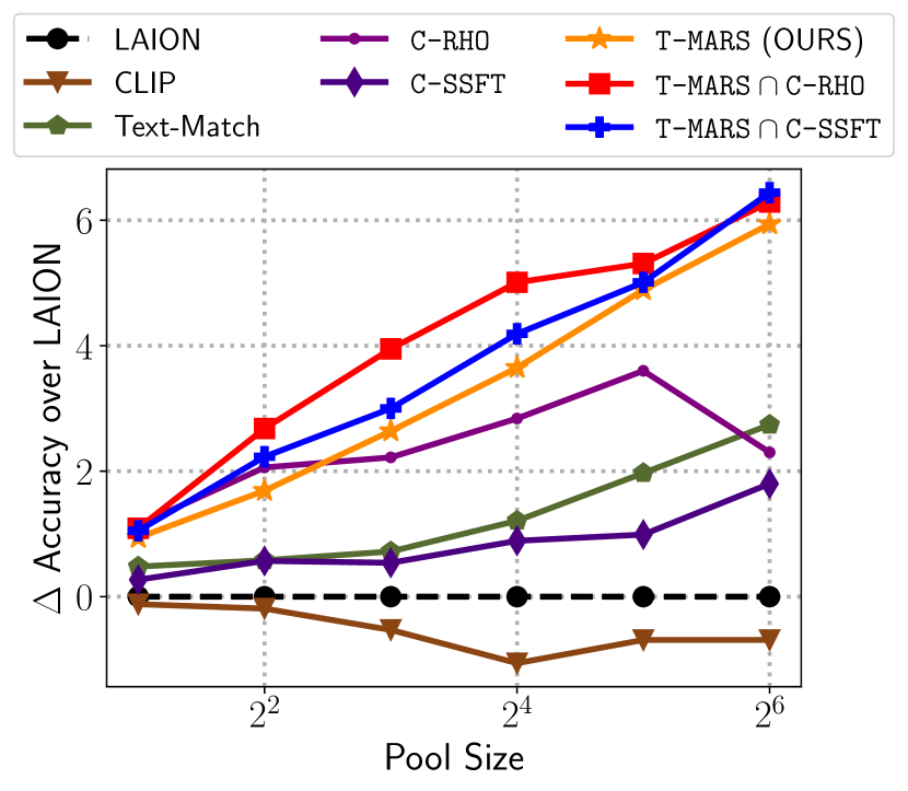
(a)

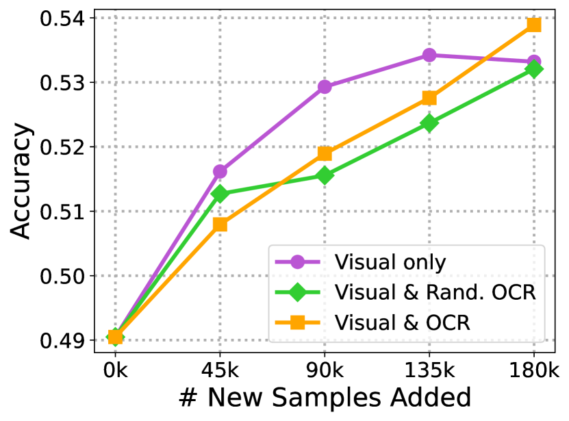
(b)

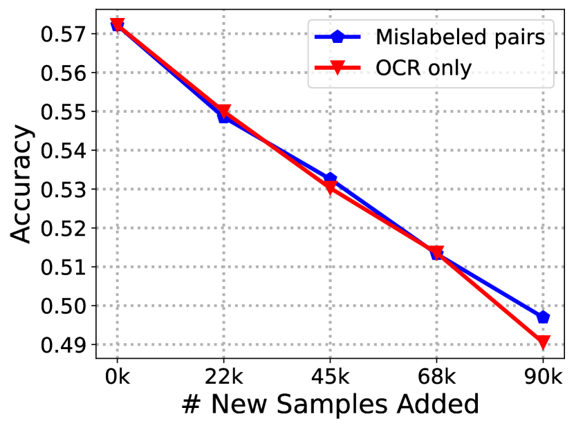
(c)

Figure 3: (a) Scaling curves depicting the increase in accuracy by training ResNet-50 models on filtered data versus training on the LAION dataset at different pool sizes. (b,c) We inspect the change in zero-shot accuracy on the Imagenette dataset when augmenting the training pool with new samples of various types. Images that contain visual features have similar utility, independent of the presence of text features; whereas those with only text features hurt as much as adding mislabeled examples.

In this section, we utilize the characterization of data types in the LAION dataset from Section 4 to simulate a similar data composition in a controlled experiment and evaluate the utility of each data type for improving visual features. We synthetically create examples of each of these types by modifying the Imagenet-Captions dataset [10].

Dataset Construction

Recall the five-fold characterization of the LAION dataset (§ 4) into samples that have images with random features ($\mathcal{S}_{r}$), useful visual features ($\mathcal{S}_{i}$), useful visual, but random OCR features ($\mathcal{S}_{irt}$), useful visual and OCR features ($\mathcal{S}_{it}$), and only useful OCR features ($\mathcal{S}_{t}$). Using the ImageNet-Captions as a base dataset, we create sample inputs for each of the five categories above. Consider an image-caption pair $({i}_{j},{t}_{j})$ from the ImageNet-Captions dataset. To create a new sample for the category $\mathcal{S}_{r}$, we replace $({i}_{j},{t}_{j})$ with $(\tilde{{i}}_{j},{t}_{j})$ by sampling $\tilde{{i}}$ from the PACS dataset ($\mathcal{S}_{\text{PACS}}$). For samples in $\mathcal{S}_{i}$, $({i}_{j},{t}_{j})$ is used as it is. Samples in $\mathcal{S}_{irt}$, are created by replacing $({i}_{j},{t}_{j})$ with $(\tilde{{i}}_{j},{t}_{j})$ by overlaying a random caption from the LAION dataset over ${{i}_{j}}$. Finally, samples in $\mathcal{S}_{it}$ and $\mathcal{S}_{t}$ are created by overlaying ${t}_{j}$ over ${i}_{j}$ or $\tilde{{i}}\sim\mathcal{S}_{\text{PACS}}$ respectively.

Experiment Protocol

Starting with a fixed data pool, we add new samples belonging to a particular data type and evaluate the accuracy of the trained model on the same. We ensure that the number of training steps is the same across all training runs (fixed at 600 steps at a batch size of 1024), and repeat and average all experimental results for 3 seeds. For results in Figure 3(b), we start with a base configuration of 180k samples from $\mathcal{S}_{i}$, and 90k samples from $\mathcal{S}_{t}$, and add varying sized subsets of new samples from $\mathcal{S}_{i},\mathcal{S}_{irt},\mathcal{S}_{it}$. For results in Figure 3(c), we start with a base configuration of 180k samples from $\mathcal{S}_{i}$, and add varying-sized subsets of new samples from $\mathcal{S}_{r},\mathcal{S}_{t}$. Note that the final configuration for $\mathcal{S}_{t}$ is the same as the initial configuration for the graphs in Figure 3(b).

We train a randomly initialized ViT-B-32 vision encoder with a pre-trained RoBERTa text encoder for 120 steps of warmup followed by a cosine schedule with a maximum learning rate of $1e^{-3}$. Evaluation is performed on the Imagenette [22] dataset (a 10-class subset of Imagenet).

Results

In the local neighborhood of a fixed compute and data budget, we observe that different data types exhibit a linear relationship between the model’s zero-shot accuracy and the number of samples from that type that are added. We define the utility of a data type at a given base configuration as $\mathcal{U}_{\text{type}}=\nicefrac{{\Delta\text{acc}}}{{\Delta\text{samples(in millions)}}}$.

1. Samples with only OCR feature ($\mathcal{U}_{t}=-0.89$) are as harmful as mislabeled ones ($\mathcal{U}_{r}=-0.8$).

2. If an image has useful visual features, then independent of the presence of useful ($\mathcal{U}_{it}=+0.27$), random ($\mathcal{U}_{irt}=+0.24$), or no OCR features ($\mathcal{U}_{i}=+0.23$), they have similar utility.

3. Removing bad examples has $3\times$ more utility than adding new good examples. This directly follows from the utility analysis of the OCR-only images, and those with visual features.

Overall, the above inferences further support the choices made in order to propose T-MARS. The utility of different data types confirms that we should retain samples that have both visual and text features in them, and naively removing all samples with text in them (such as in recent work by Radenovic et al. [39]) is a sub-optimal strategy. Secondly, our results suggest that while scaling up data sizes has been a useful recipe for improving the quality of visual representation, the community should also focus on pruning off so-called ‘bad examples’ from the datasets, because pruning bad examples is significantly more useful than adding more examples.

8 Conclusion and Limitations

In this work, we introduced a state-of-the-art data curation approach that significantly improves visual representation learning in vision-language models like CLIP. Our proposed approach is based on the interesting observation that a large fraction of image-caption pairs in web-scale datasets contain images dominated by text features. filters out such images as they encourage the model to learn the orthogonal task of optical character recognition (OCR) rather than helping towards learning better visual representations. On the recently released data filtering competition DataComp, outperforms the top of the leaderboard (medium data scale) by 6.5%. Notably, our scaling trends of accuracy gains over the baselines show a linear increase in gains as the data pool size is increased exponentially. This makes a promising case for observing strong gains at even higher data scales. Our work contributes to advancing the understanding of data filtering in web-scale datasets and highlights the significance of high-quality data curation as the scale of data increases.

While in this work, we create a static subset of the original corpus and perform multiple epoch training over the same, future work may benefit by assessing the utility of different data points in a dynamic fashion and refreshing the data pool with samples worth learning. This involves assessing the utility of samples (and that too, in a computationally efficient way), as easy examples might have a large drop in utility after only a small number of epochs compared to hard examples.

A trade-off of training on filtered data is that such CLIP models do not have OCR capabilities. We remark that (i) the OCR capabilities of the original CLIP models is already very weak, and the specialized task of OCR can be solved more accurately via direct approaches tailored for text recognition; and (ii) the family of CLIP models is used as a de-facto standard for visual representations rather than OCR. Finally, we note that data subset selection can introduce or amplify biases, particularly those that affect marginalized sub-populations. We don’t see any immediate harmful biases introduced by our specific approach because we only remove images that do not contribute much towards visual representation learning.

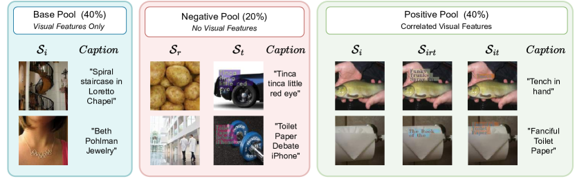
Figure 4: A representation of the various pools of data created for the synthetic experiments that evaluate example utility.

Appendix A Synthetic Experiment Setup Details

For each example $j$, the dataset contains image ($x_{j}$), title ($y_{j}$), and metadata ($m_{j}$). We create image-caption pairs, $({i}_{j},{t}_{j})=(x_{j},\texttt{"Title: \{}y_{j}\texttt{\} | Metadata: \{}m_{j}\texttt{\}"}$ for each example. Then, depending on the category of data that a particular example should belong to, we modify the input in the following way:

1. $\mathcal{S}_{r}$: $({i}_{j},{t}_{j})$ is replaced with $(\tilde{{i}}_{j},{t}_{j})$ by sampling $\tilde{{i}}$ from the PACS dataset.

2. $\mathcal{S}_{i}$: $({i}_{j},{t}_{j})$ is used as it is.

3. $\mathcal{S}_{irt}$: $({i}_{j},{t}_{j})$ is replaced with $(\tilde{{i}}_{j},{t}_{j})$ by overlaying the first four words of a random caption from the LAION dataset over ${{i}_{j}}$.

4. $\mathcal{S}_{it}$: $({i}_{j},{t}_{j})$ is replaced with $(\tilde{{i}}_{j},{t}_{j})$ by overlaying the title corresponding to ${t}_{j}$ on ${i}_{j}$.

5. $\mathcal{S}_{t}$: $({i}_{j},{t}_{j})$ is replaced with $(\tilde{{i}}_{j},{t}_{j})$ by overlaying the title corresponding to ${t}_{j}$ on a random image sampled from the PACS dataset.

Creating Dataset Pool

An important consideration for any controlled experiment is to make sure that the effect of adding different types of examples is compared by generating variants of the same example across different types. That is, when adding new samples from $\mathcal{S}_{i},\mathcal{S}_{irt},\mathcal{S}_{it}$, we want to ensure that they are variants of the same source example $({i}_{j},{t}_{j})$. Similarly, we want to ensure the same when we remove examples from $\mathcal{S}_{r},\mathcal{S}_{t}$ as well.

1. Base Data Pool: This is a sample of 40% of the Imagenet-Captions Dataset, and only contains samples belonging to $\mathcal{S}_{i}$. An illustration of the same is presented in panel 1 of Figure 4.

2. Negative Pool: This is a sample of 20% of the Imagenet-Captions Dataset. For each example (${i}_{j},{t}_{j}$) we create two copies of the sample for the types that do not contain any visual features—$\mathcal{S}_{r},\mathcal{S}_{t}$. An illustration of the same is presented in panel 2 of Figure 4. The caption is preserved, but the images are either substituted with a random image (as in the case of $\mathcal{S}_{r}$), or with a random image with the title overlayed (as in the case of $\mathcal{S}_{t}$).

3. Positive Pool: This is a sample of the remaining 40% image-caption pairs from the Imagenet-Captions Dataset. For each example (${i}_{j},{t}_{j}$) we create three copies of the sample for the types containing visual features—$\mathcal{S}_{i},\mathcal{S}_{irt},\mathcal{S}_{it}$. An illustration of the same is presented in panel 3 of Figure 4. The caption is preserved, but the images are either overlayed with a random text (as in the case of $\mathcal{S}_{irt}$), or with the caption title (as in the case of $\mathcal{S}_{it}$).

Experiment Configuration

The base data pool is used for all experiments. For experiments that evaluate the utility of random, and text-only images, we add new samples from the corresponding negative pool and evaluate the zero-shot accuracy of the model on the Imagenette [22] dataset. For experiments that evaluate the utility of images that contain visual features, our base training set comprises all image-caption pairs from the base data pool (40%) and all image-caption pairs from the text-only (negative) pool (20%). This is done in order to ensure that the model has the incentive to learn text features in order to perform well on the pre-training task. Only then can we evaluate if adding images with text features is hurtful to the model’s learning or not? In the absence of text-only images, we find that the model is able to easily treat the text features as random features, defeating the purpose of the experiment. Finally, we add varying fractions of image-caption pairs from the positive pool to evaluate the utility of each data type. Results for the same are presented in the main paper in Figure 3.

Appendix B Data removed by various curation approches

B.1 Hyper-parameter search for baselines

An important question that arises when using score-based filtering metrics like C-RHO , C-SSFT and is how to select the score threshold above which a sample is retained, which consequently dictates the filtered subset size. In our experiments, for the 3 data filtering metrics above, we did a hyper-parameter search over filtered subset size in the grid $\{90\%,75\%,60\%,50\%\}$ of the original unfiltered pool size. For C-SSFT , retaining $90\%$ samples i.e. removing only $10\%$ of the data worked the best, which is in line with the observations in  Maini et al. [34]. For C-RHO and , we observe that filtering out $50\%$ of the data worked the best. For Text-Matching, we used the criteria of  Radenovic et al. [39], where a sample is filtered out if 5 characters in OCR match with the caption.

Table 3: Analysis of the fraction of image-caption pairs from different types that were retained by each filtering algorithm studied in our paper, assessed based on a 500-example pilot study. The first column presents the total number of images from each category in the subset of the LAION dataset.

	Total	Text-
Image-Caption Category	Images	Match	C-SSFT	C-RHO		$\cap$ C-SSFT	$\cap$ C-RHO
Random ($\mathcal{S}_{r}$)	18	1.00	0.59	0.41	0.29	0.24	0.12
Visual only ($\mathcal{S}_{i}$)	234	0.99	0.89	0.60	0.67	0.60	0.37
Visual, Random OCR ($\mathcal{S}_{irt}$)	49	0.89	0.80	0.62	0.71	0.51	0.42
Visual & OCR ($\mathcal{S}_{it}$)	96	0.22	0.93	0.65	0.48	0.45	0.30
OCR only ($\mathcal{S}_{t}$)	103	0.08	0.91	0.46	0.07	0.07	0.04

B.2 Visualizing the data removed

Recall in Section 6.4, we discussed the number of samples removed by various filtering metrics from each category in our 500 image pilot study. Table 3 lists the fraction of samples from each category retained by various metrics. Figure 5 shows the images that were filtered out by text matching metric but retained by . Recall that these would correspond to the cases where both the visual and text features are correlated with the caption. Figure 6 shows the images that were filtered out by both metrics. Finally, in Figure 7, Figure 8, Figure 9 and Figure 10 we share some of the samples removed by C-SSFT and C-RHO metrics.

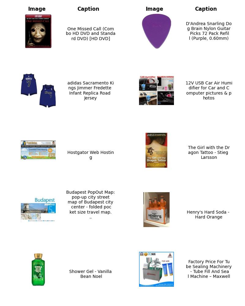
Figure 5: Samples removed by Text-Matching but retained by our proposed approach . These correspond to the images where both the visual and text features are correlated with the caption

.

Figure 6: Samples removed by both text-matching and . Here only the text features are correlated with the caption

.

Figure 7: Samples with the lowest score (and filtered out) based on the C-SSFT metric

.

Figure 8: Additional (random) samples filtered out by the C-SSFT metric

.

Figure 9: Samples with the lowest score (and filtered out) based on the C-RHO metric

.

Figure 10: Additional (random) samples filtered out by the C-RHO metric

.

B.3 Failure Cases for Text-Matching

Recall that text-matching requires to recognize the text, which is upto an order of magnitude more compute expensive than text-detection. However, additionaly we observe that text-recognition has a lot of failure cases as well, where although the text is detected correctly, but the recognition process fails to read correctly, as shown in Figure 11. In line with the previous works [39], we used the MMOCR library for text-recognition. These failure modes maybe addressed with the use of much more expensive transformer based text-recognition models like Text Spotting Transformers, albeit at a prohibitively high cost for webscales considered in this work.

Figure 11: Some failure cases of text-matching, due to failure of the text recognition process. All these images have text overlapping with the caption and should have been filtered out ideally, but end up being retained as the text recognition fails to read the text correctly.

.

Appendix C Additional Results on LAION

Table 4: Zero-shot accuracies for models trained on filtered subsets of the original LAION dataset when evaluated on a suite of 17 benchmark datasets (§ 6.2). Rows in ‘orange’ depict previous baselines (§ 5.3), those in ‘white’ depict our contributed baselines (§ 5.2), and those in ‘green’ depict our state-of-the-art method (§ 5). $\cap$ denotes the intersection between two filtering strategies.

			ResNet-50				ViT-B-32
		Dataset		ImageNet				ImageNet
Scale	Filtering	size	ImageNet	dist. shifts	VTAB	Retrieval	ImageNet	dist. shifts	VTAB	Retrieval
	LAION	100%	02.57	03.50	14.82	09.27	01.21	02.04	13.42	08.23
	CLIP Score (@ 50%)	50.0%	02.46	03.62	14.61	10.09	01.26	02.40	13.75	07.92
	Text-Match	86.4%	03.05	03.78	15.97	09.28	01.35	02.45	13.05	08.90
	C-SSFT	90.0%	02.85	03.65	15.41	09.64	01.38	02.38	14.96	08.76
	C-RHO	50.0%	03.70	04.41	15.67	10.84	01.46	02.54	14.85	09.25
		50.0%	03.51	04.18	14.86	10.87	01.40	02.41	12.98	09.77
	$\cap$ C-SSFT	45.2%	03.62	04.48	16.59	09.98	01.60	02.61	14.72	09.59
2M	$\cap$ C-RHO	27.5%	03.70	04.58	16.80	10.20	01.72	02.77	14.79	09.63
	LAION	100%	07.06	07.06	17.79	11.72	03.05	03.79	16.18	10.00
	CLIP Score (@ 50%)	50.0%	06.86	07.40	18.07	11.95	03.20	04.00	15.71	09.36
	Text-Match	86.4%	07.66	07.39	18.42	12.28	03.51	04.30	16.70	09.60
	C-SSFT	90.0%	07.64	07.44	18.94	12.22	03.42	04.19	16.66	09.73
	C-RHO	50.0%	09.12	08.67	20.73	13.73	03.60	04.34	16.38	10.63
		50.0%	08.77	08.69	20.94	13.67	04.04	04.64	17.10	11.59
	$\cap$ C-SSFT	45.2%	09.30	08.80	19.12	13.45	04.22	04.63	17.04	11.27
4M	$\cap$ C-RHO	27.5%	09.75	09.20	21.41	14.17	04.28	05.05	16.20	11.69
	LAION	100%	11.62	10.77	21.74	14.02	05.57	05.81	17.32	10.95
	CLIP Score (@ 50%)	50.0%	11.13	10.60	21.87	13.88	05.80	05.92	17.45	10.90
	Text-Match	86.4%	12.38	11.35	22.64	14.03	06.16	06.19	17.89	10.94
	C-SSFT	90.0%	12.19	11.36	20.88	14.54	05.92	06.22	17.60	11.21
	C-RHO	50.0%	13.86	12.94	22.12	15.90	06.55	06.43	18.55	11.77
		50.0%	14.10	12.97	22.20	16.05	07.20	07.28	19.02	12.83
	$\cap$ C-SSFT	45.2%	14.65	13.01	22.35	16.10	07.54	07.22	19.18	12.66
8M	$\cap$ C-RHO	27.5%	15.60	13.09	22.85	16.33	07.65	07.39	18.63	13.17
	LAION	100%	16.63	15.04	24.20	16.79	09.39	08.46	19.83	12.58
	CLIP Score (@ 50%)	50.0%	15.58	14.28	23.67	16.28	09.02	08.42	20.13	12.60
	Text-Match	86.4%	17.83	15.83	24.63	17.11	10.16	08.89	20.63	12.84
	C-SSFT	90.0%	17.49	15.61	24.90	17.31	10.10	08.94	19.67	13.26
	C-RHO	50.0%	19.46	17.39	26.45	18.60	10.87	09.34	21.22	13.93
		50.0%	20.25	17.71	26.50	18.45	12.09	10.35	22.64	14.15
	$\cap$ C-SSFT	45.2%	20.81	18.28	26.49	18.96	12.56	10.60	21.96	14.36
16M	$\cap$ C-RHO	27.5%	21.63	18.62	26.70	19.53	12.61	10.94	23.48	14.58
	LAION	100%	21.90	18.90	27.30	20.18	14.98	12.38	23.21	16.03
	CLIP Score (@ 50%)	50.0%	20.84	18.79	25.71	19.54	14.69	12.86	22.81	15.32
	Text-Match	86.4%	23.80	20.70	28.74	21.41	15.96	13.26	24.45	16.44
	C-SSFT	90.0%	22.87	19.85	26.10	21.00	15.55	13.34	22.95	16.40
	C-RHO	50.0%	25.44	21.81	27.65	22.61	16.76	13.98	25.60	17.48
		50.0%	26.73	22.79	29.88	22.62	18.75	15.30	26.71	16.82
	$\cap$ C-SSFT	45.2%	26.89	22.83	28.81	22.99	19.18	15.86	27.13	17.82
32M	$\cap$ C-RHO	27.5%	27.20	23.30	30.30	22.77	19.15	15.86	26.93	18.04
	LAION	100%	26.34	23.24	29.09	23.91	20.37	17.97	27.85	18.83
	CLIP Score (@ 50%)	50.0%	25.66	22.83	29.05	23.36	20.07	17.27	27.55	18.33
	Text-Match	86.4%	29.11	24.94	30.35	25.75	23.11	19.04	28.82	19.37
	C-SSFT	90.0%	28.15	24.13	29.73	25.58	21.80	18.20	27.69	19.54
	C-RHO	50.0%	28.66	24.83	30.13	19.79	23.27	19.23	27.94	21.10
		50.0%	32.47	27.52	33.05	24.99	25.78	21.05	31.69	20.52
	$\cap$ C-SSFT	45.2%	32.77	27.68	33.13	26.35	25.63	21.01	30.02	21.27
64M	$\cap$ C-RHO	27.5%	32.63	27.23	32.77	25.57	25.62	20.73	31.57	20.63

Recall that in Section 6.3, we observed a linear scaling trend of zeroshot accuracies as we varied the pool size (LAION subset) from 2M to 64M. In Table 4, we share the detailed zeroshot accuracies for models trained on various subsets.

References

- [1] Common crawl. https://commoncrawl.org/.
- Abbas et al. [2023] Amro Abbas, Kushal Tirumala, Dániel Simig, Surya Ganguli, and Ari S Morcos. Semdedup: Data-efficient learning at web-scale through semantic deduplication. arXiv preprint arXiv:2303.09540, 2023.
- Agarwal et al. [2003] Pankaj Agarwal, Sariel Har-peled, and Kasturi Varadarajan. Approximating extent measures of points. Journal of the ACM, 51, 03 2003. doi: 10.1145/1008731.1008736.
- Barbu et al. [2019] Andrei Barbu, David Mayo, Julian Alverio, William Luo, Christopher Wang, Dan Gutfreund, Josh Tenenbaum, and Boris Katz. Objectnet: A large-scale bias-controlled dataset for pushing the limits of object recognition models. In Advances in Neural Information Processing Systems (NeurIPS), pages 9453–9463, 2019.
- Carlini et al. [2019] Nicholas Carlini, Úlfar Erlingsson, and Nicolas Papernot. Distribution density, tails, and outliers in machine learning: Metrics and applications. ArXiv, abs/1910.13427, 2019.
- Chatterjee [2020] Satrajit Chatterjee. Coherent gradients: An approach to understanding generalization in gradient descent-based optimization. arXiv preprint arXiv:2002.10657, 2020.
- Chen et al. [2022] Xi Chen, Xiao Wang, Soravit Changpinyo, AJ Piergiovanni, Piotr Padlewski, Daniel Salz, Sebastian Goodman, Adam Grycner, Basil Mustafa, Lucas Beyer, et al. Pali: A jointly-scaled multilingual language-image model. arXiv preprint arXiv:2209.06794, 2022.
- Chen et al. [2021] Zhe Chen, Jiahao Wang, Wenhai Wang, Guo Chen, Enze Xie, Ping Luo, and Tong Lu. Fast: Faster arbitrarily-shaped text detector with minimalist kernel representation, 2021.
- Clark et al. [2022] Aidan Clark, Diego de las Casas, Aurelia Guy, Arthur Mensch, Michela Paganini, Jordan Hoffmann, Bogdan Damoc, Blake Hechtman, Trevor Cai, Sebastian Borgeaud, George van den Driessche, Eliza Rutherford, Tom Hennigan, Matthew Johnson, Katie Millican, Albin Cassirer, Chris Jones, Elena Buchatskaya, David Budden, Laurent Sifre, Simon Osindero, Oriol Vinyals, Jack Rae, Erich Elsen, Koray Kavukcuoglu, and Karen Simonyan. Unified scaling laws for routed language models, 2022.
- Fang et al. [2022] Alex Fang, Gabriel Ilharco, Mitchell Wortsman, Yuhao Wan, Vaishaal Shankar, Achal Dave, and Ludwig Schmidt. Data determines distributional robustness in contrastive language image pre-training (clip). In International Conference on Machine Learning, pages 6216–6234. PMLR, 2022.
- Feldman et al. [2011] Dan Feldman, Matthew Faulkner, and Andreas Krause. Scalable training of mixture models via coresets. In J. Shawe-Taylor, R. Zemel, P. Bartlett, F. Pereira, and K.Q. Weinberger, editors, Advances in Neural Information Processing Systems, volume 24. Curran Associates, Inc., 2011. URL https://proceedings.neurips.cc/paper_files/paper/2011/file/2b6d65b9a9445c4271ab9076ead5605a-Paper.pdf.
- Feldman [2020] Vitaly Feldman. Does learning require memorization? a short tale about a long tail. Proceedings of the 52nd Annual ACM SIGACT Symposium on Theory of Computing, 2020.
- Feldman and Zhang [2020] Vitaly Feldman and Chiyuan Zhang. What neural networks memorize and why: Discovering the long tail via influence estimation. Advances in Neural Information Processing Systems, 33:2881–2891, 2020.
- Gadre et al. [2023] Samir Yitzhak Gadre, Gabriel Ilharco, Alex Fang, Jonathan Hayase, Georgios Smyrnis, Thao Nguyen, Ryan Marten, Mitchell Wortsman, Dhruba Ghosh, Jieyu Zhang, Eyal Orgad, Rahim Entezari, Giannis Daras, Sarah Pratt, Vivek Ramanujan, Yonatan Bitton, Kalyani Marathe, Stephen Mussmann, Richard Vencu, Mehdi Cherti, Ranjay Krishna, Pang Wei Koh, Olga Saukh, Alexander Ratner, Shuran Song, Hannaneh Hajishirzi, Ali Farhadi, Romain Beaumont, Sewoong Oh, Alex Dimakis, Jenia Jitsev, Yair Carmon, Vaishaal Shankar, and Ludwig Schmidt. Datacomp: In search of the next generation of multimodal datasets, 2023.
- Goyal et al. [2022] Sachin Goyal, Ananya Kumar, Sankalp Garg, Zico Kolter, and Aditi Raghunathan. Finetune like you pretrain: Improved finetuning of zero-shot vision models, 2022.
- Har-Peled and Mazumdar [2004] Sariel Har-Peled and Soham Mazumdar. On coresets for k-means and k-median clustering. In Symposium on the Theory of Computing, 2004.
- Hendrycks et al. [2019] Dan Hendrycks, Kevin Zhao, Steven Basart, Jacob Steinhardt, and Dawn Song. Natural adversarial examples. arXiv preprint arXiv:1907.07174, 2019.
- Hendrycks et al. [2020] Dan Hendrycks, Steven Basart, Norman Mu, Saurav Kadavath, Frank Wang, Evan Dorundo, Rahul Desai, Tyler Zhu, Samyak Parajuli, Mike Guo, Dawn Song, Jacob Steinhardt, and Justin Gilmer. The many faces of robustness: A critical analysis of out-of-distribution generalization. arXiv preprint arXiv:2006.16241, 2020.
- Hernandez et al. [2021] Danny Hernandez, Jared Kaplan, Tom Henighan, and Sam McCandlish. Scaling laws for transfer, 2021.
- Hestness et al. [2017] Joel Hestness, Sharan Narang, Newsha Ardalani, Gregory Diamos, Heewoo Jun, Hassan Kianinejad, Md. Mostofa Ali Patwary, Yang Yang, and Yanqi Zhou. Deep learning scaling is predictable, empirically, 2017.
- Hoffmann et al. [2022] Jordan Hoffmann, Sebastian Borgeaud, Arthur Mensch, Elena Buchatskaya, Trevor Cai, Eliza Rutherford, Diego de Las Casas, Lisa Anne Hendricks, Johannes Welbl, Aidan Clark, et al. Training compute-optimal large language models. arXiv preprint arXiv:2203.15556, 2022.
- [22] Jeremy Howard. Imagenette. URL https://github.com/fastai/imagenette/.
- Ilharco et al. [2021] Gabriel Ilharco, Mitchell Wortsman, Ross Wightman, Cade Gordon, Nicholas Carlini, Rohan Taori, Achal Dave, Vaishaal Shankar, Hongseok Namkoong, John Miller, Hannaneh Hajishirzi, Ali Farhadi, and Ludwig Schmidt. Openclip, July 2021. URL https://doi.org/10.5281/zenodo.5143773. If you use this software, please cite it as below.
- Jia et al. [2021] Chao Jia, Yinfei Yang, Ye Xia, Yi-Ting Chen, Zarana Parekh, Hieu Pham, Quoc Le, Yun-Hsuan Sung, Zhen Li, and Tom Duerig. Scaling up visual and vision-language representation learning with noisy text supervision. In International Conference on Machine Learning, pages 4904–4916. PMLR, 2021.
- Jiang et al. [2001] Mon-Fong Jiang, Shian-Shyong Tseng, and Chih-Ming Su. Two-phase clustering process for outliers detection. Pattern Recognition Letters, 22:691–700, 01 2001.
- Jiang et al. [2020] Ziheng Jiang, Chiyuan Zhang, Kunal Talwar, and Michael C Mozer. Characterizing structural regularities of labeled data in overparameterized models. arXiv preprint arXiv:2002.03206, 2020.
- Kaplan et al. [2020] Jared Kaplan, Sam McCandlish, Tom Henighan, Tom B. Brown, Benjamin Chess, Rewon Child, Scott Gray, Alec Radford, Jeffrey Wu, and Dario Amodei. Scaling laws for neural language models, 2020.
- Kaplun et al. [2022] Gal Kaplun, Nikhil Ghosh, Saurabh Garg, Boaz Barak, and Preetum Nakkiran. Deconstructing distributions: A pointwise framework of learning. arXiv preprint arXiv:2202.09931, 2022.
- Kumar et al. [2022] Ananya Kumar, Aditi Raghunathan, Robbie Jones, Tengyu Ma, and Percy Liang. Fine-tuning can distort pretrained features and underperform out-of-distribution. In International Conference on Learning Representations (ICLR), 2022.
- Lee et al. [2022] Katherine Lee, Daphne Ippolito, Andrew Nystrom, Chiyuan Zhang, Douglas Eck, Chris Callison-Burch, and Nicholas Carlini. Deduplicating training data makes language models better, 2022.
- Li et al. [2021] Junnan Li, Ramprasaath Selvaraju, Akhilesh Gotmare, Shafiq Joty, Caiming Xiong, and Steven Chu Hong Hoi. Align before fuse: Vision and language representation learning with momentum distillation. Advances in neural information processing systems, 34:9694–9705, 2021.
- Li et al. [2020] Xiujun Li, Xi Yin, Chunyuan Li, Pengchuan Zhang, Xiaowei Hu, Lei Zhang, Lijuan Wang, Houdong Hu, Li Dong, Furu Wei, et al. Oscar: Object-semantics aligned pre-training for vision-language tasks. In Computer Vision–ECCV 2020: 16th European Conference, Glasgow, UK, August 23–28, 2020, Proceedings, Part XXX 16, pages 121–137. Springer, 2020.
- Li et al. [2022] Yangguang Li, Feng Liang, Lichen Zhao, Yufeng Cui, Wanli Ouyang, Jing Shao, Fengwei Yu, and Junjie Yan. Supervision exists everywhere: A data efficient contrastive language-image pre-training paradigm, 2022.
- Maini et al. [2022] Pratyush Maini, Saurabh Garg, Zachary Chase Lipton, and J Zico Kolter. Characterizing datapoints via second-split forgetting. In Alice H. Oh, Alekh Agarwal, Danielle Belgrave, and Kyunghyun Cho, editors, Advances in Neural Information Processing Systems, 2022. URL https://openreview.net/forum?id=yKDKNzjHg8N.
- Mangalam and Prabhu [2019] Karttikeya Mangalam and Vinay Uday Prabhu. Do deep neural networks learn shallow learnable examples first? In ICML 2019 Workshop on Identifying and Understanding Deep Learning Phenomena, 2019. URL https://openreview.net/forum?id=HkxHv4rn24.
- Mindermann et al. [2022] Sören Mindermann, Jan M Brauner, Muhammed T Razzak, Mrinank Sharma, Andreas Kirsch, Winnie Xu, Benedikt Höltgen, Aidan N Gomez, Adrien Morisot, Sebastian Farquhar, et al. Prioritized training on points that are learnable, worth learning, and not yet learnt. In International Conference on Machine Learning, pages 15630–15649. PMLR, 2022.
- Mu et al. [2021] Norman Mu, Alexander Kirillov, David Wagner, and Saining Xie. Slip: Self-supervision meets language-image pre-training, 2021.
- Pham et al. [2021] Hieu Pham, Zihang Dai, Golnaz Ghiasi, Kenji Kawaguchi, Hanxiao Liu, Adams Wei Yu, Jiahui Yu, Yi-Ting Chen, Minh-Thang Luong, Yonghui Wu, et al. Combined scaling for zero-shot transfer learning. arXiv preprint arXiv:2111.10050, 2021.
- Radenovic et al. [2023] Filip Radenovic, Abhimanyu Dubey, Abhishek Kadian, Todor Mihaylov, Simon Vandenhende, Yash Patel, Yi Wen, Vignesh Ramanathan, and Dhruv Mahajan. Filtering, distillation, and hard negatives for vision-language pre-training. arXiv:2301.02280, 2023.
- Radford et al. [2021] Alec Radford, Jong Wook Kim, Chris Hallacy, Aditya Ramesh, Gabriel Goh, Sandhini Agarwal, Girish Sastry, Amanda Askell, Pamela Mishkin, Jack Clark, Gretchen Krueger, and Ilya Sutskever. Learning transferable visual models from natural language supervision. In International Conference on Machine Learning (ICML), volume 139, pages 8748–8763, 2021.
- Raffel et al. [2020] Colin Raffel, Noam Shazeer, Adam Roberts, Katherine Lee, Sharan Narang, Michael Matena, Yanqi Zhou, Wei Li, and Peter J. Liu. Exploring the limits of transfer learning with a unified text-to-text transformer, 2020.
- Recht et al. [2019] Benjamin Recht, Rebecca Roelofs, Ludwig Schmidt, and Vaishaal Shankar. Do imagenet classifiers generalize to imagenet? In International Conference on Machine Learning (ICML), 2019.
- Rousseeuw and Hubert [2018] Peter Rousseeuw and Mia Hubert. Anomaly detection by robust statistics. Wiley Interdisciplinary Reviews: Data Mining and Knowledge Discovery, 8, 03 2018. doi: 10.1002/widm.1236.
- Russakovsky et al. [2015] Olga Russakovsky, Jia Deng, Hao Su, Jonathan Krause, Sanjeev Satheesh, Sean Ma, Zhiheng Huang, Andrej Karpathy, Aditya Khosla, Michael Bernstein, Alexander C. Berg, and Li Fei-Fei. Imagenet large scale visual recognition challenge, 2015.
- Schuhmann et al. [2021] Christoph Schuhmann, Richard Vencu, Romain Beaumont, Robert Kaczmarczyk, Clayton Mullis, Aarush Katta, Theo Coombes, Jenia Jitsev, and Aran Komatsuzaki. Laion-400m: Open dataset of clip-filtered 400 million image-text pairs, 2021.
- Schuhmann et al. [2022] Christoph Schuhmann, Romain Beaumont, Richard Vencu, Cade Gordon, Ross Wightman, Mehdi Cherti, Theo Coombes, Aarush Katta, Clayton Mullis, Mitchell Wortsman, et al. Laion-5b: An open large-scale dataset for training next generation image-text models. arXiv preprint arXiv:2210.08402, 2022.
- Shah et al. [2020] Harshay Shah, Kaustav Tamuly, Aditi Raghunathan, Prateek Jain, and Praneeth Netrapalli. The pitfalls of simplicity bias in neural networks. Advances in Neural Information Processing Systems, 33:9573–9585, 2020.
- Sorscher et al. [2023] Ben Sorscher, Robert Geirhos, Shashank Shekhar, Surya Ganguli, and Ari S. Morcos. Beyond neural scaling laws: beating power law scaling via data pruning, 2023.
- Wang et al. [2019] Haohan Wang, Songwei Ge, Zachary Lipton, and Eric P Xing. Learning robust global representations by penalizing local predictive power. In Advances in Neural Information Processing Systems (NeurIPS), 2019.
- Wang et al. [2021] Zirui Wang, Jiahui Yu, Adams Wei Yu, Zihang Dai, Yulia Tsvetkov, and Yuan Cao. Simvlm: Simple visual language model pretraining with weak supervision. arXiv preprint arXiv:2108.10904, 2021.
- Wortsman et al. [2021] Mitchell Wortsman, Gabriel Ilharco, Mike Li, Jong Wook Kim, Hannaneh Hajishirzi, Ali Farhadi, Hongseok Namkoong, and Ludwig Schmidt. Robust fine-tuning of zero-shot models. arXiv preprint arXiv:2109.01903, 2021.
- Xu et al. [2023] Hu Xu, Saining Xie, Po-Yao Huang, Licheng Yu, Russell Howes, Luke Zettlemoyer Gargi Ghosh, and Christoph Feichtenhofer. Cit: Curation in training for effective vision-language data. arXiv preprint arXiv:2301.02241, 2023.
- Yao et al. [2021] Lewei Yao, Runhui Huang, Lu Hou, Guansong Lu, Minzhe Niu, Hang Xu, Xiaodan Liang, Zhenguo Li, Xin Jiang, and Chunjing Xu. Filip: fine-grained interactive language-image pre-training. arXiv preprint arXiv:2111.07783, 2021.
- Yu et al. [2002] Dantong Yu, Gholamhosein Sheikholeslami, and Aidong Zhang. Findout: Finding outliers in very large datasets. Knowl. Inf. Syst., 4:387–412, 09 2002. doi: 10.1007/s101150200013.
- Zhai et al. [2020] Xiaohua Zhai, Joan Puigcerver, Alexander Kolesnikov, Pierre Ruyssen, Carlos Riquelme, Mario Lucic, Josip Djolonga, Andre Susano Pinto, Maxim Neumann, Alexey Dosovitskiy, Lucas Beyer, Olivier Bachem, Michael Tschannen, Marcin Michalski, Olivier Bousquet, Sylvain Gelly, and Neil Houlsby. A large-scale study of representation learning with the visual task adaptation benchmark, 2020.
- Zhai et al. [2022] Xiaohua Zhai, Alexander Kolesnikov, Neil Houlsby, and Lucas Beyer. Scaling vision transformers, 2022.