Unobstructed Lagrangian cobordism groups of surfaces

Abstract.

We study Lagrangian cobordism groups of closed symplectic surfaces of genus $g\geq 2$ whose relations are given by unobstructed, immersed Lagrangian cobordisms. Building upon work of Abouzaid [Abo08] and Perrier [Per19], we compute these cobordism groups and show that they are isomorphic to the Grothendieck group of the derived Fukaya category of the surface.

1. Introduction

Lagrangian cobordism is a relation between Lagrangian submanifolds of a symplectic manifold $(M,\omega)$ that was introduced by Arnold [Arn80]. A consequence of the Gromov-Lees h-principle is that the study of general immersed Lagrangian cobordisms essentially reduces to algebraic topology, see [Eli84, Aud87]. In contrast, cobordisms satisfying suitable geometric constraints display remarkable rigidity phenomena. A fundamental example of this is the proof by Biran and Cornea [BC13, BC14] that monotone, embedded Lagrangian cobordisms give rise to cone decompositions in the derived Fukaya category $\operatorname{DFuk}(M)$. See also [BC17, BCS21, BC21] for further developments, as well as the work of Nadler and Tanaka [NT20], who obtained related results from a different perspective.

A natural problem is to establish to what extent Lagrangian cobordisms determine the structure of $\operatorname{DFuk}(M)$. In this paper, we consider the following formalization of this question. Fix classes of Lagrangians in $M$ and of Lagrangian cobordisms in $\mathbb{C}\times M$, possibly equipped with extra structures (the precise classes considered in this paper will be specified shortly). The associated Lagrangian cobordism group $\Omega(M)$ is the abelian group whose elements are formal sums of Lagrangians in $M$, modulo relations coming from Lagrangian cobordisms. On the side of $\operatorname{DFuk}(M)$, part of the information about cone decompositions is encoded in the Grothendieck group $K_{0}\operatorname{DFuk}(M)$. (See Section 2 for precise definitions of $\Omega(M)$ and $K_{0}\operatorname{DFuk}(M)$.)

Whenever the cone decompositions results of [BC14] can be extended to the classes of Lagrangians under consideration, there is an induced surjective morphism

$$\Theta:\Omega(M)\to K_{0}\operatorname{DFuk}(M),$$

see [BC14, Corollary 1.2.1]. Biran and Cornea posed the following question.

Question 1.

When is the map $\Theta$ an isomorphism?

There are only two cases for which $\Theta$ is known to be an isomorphism (for appropriate classes of Lagrangians): the torus $T^{2}$ by work of Haug [Hau15] (see also [Hen20] for a refinement of this result), and Liouville surfaces by work of Bosshard [Bos21].

In this paper, we consider this problem in the case of a closed surface $\Sigma$ of genus $g\geq 2$. In this case, the group $K_{0}\operatorname{DFuk}(\Sigma)$ was computed by Abouzaid [Abo08], who showed that there is an isomorphism

$$K_{0}\operatorname{DFuk}(\Sigma)\cong H_{1}(S\Sigma;\mathbb{Z})\oplus\mathbb{R},$$ (1)

where $S\Sigma$ is the unit tangent bundle of $\Sigma$. The main goal of this paper is to answer Question 1 by exhibiting a Lagrangian cobordism group $\Omega_{\operatorname{unob}}(\Sigma)$ whose relations are given by unobstructed immersed cobordisms, such that the associated map $\Theta:\Omega_{\operatorname{unob}}(\Sigma)\to K_{0}\operatorname{DFuk}(\Sigma)$ is an isomorphism.

1.1. Main results

1.1.1. Unobstructed cobordisms and cone decompositions

Our first main result is an extension of the cone decomposition results of [BC14] to a class of immersed Lagrangian cobordisms that are unobstructed, in the sense that they have a well-behaved Floer theory. There exist many different mechanisms to achieve unobstructedness in the litterature, at varying levels of generality and technical complexity; see Remark 1.3 for a discussion. The precise notion of unobstructedness considered in this work is the following: we say that an immersed Lagrangian cobordism is quasi-exact if it does not bound $J$-holomorphic disks and teardrops for suitable almost complex structures $J$ (see Section 3.2 for the precise definition). In this work, we will use the terms quasi-exact and unobstructed interchangeably.

To state the first theorem, we let $(M,\omega)$ be a closed symplectic manifold which is symplectically aspherical, in the sense that $\omega|_{\pi_{2}(M)}=0$. Recall that a Lagrangian submanifold $L\subset M$ is called weakly exact if $\omega|_{\pi_{2}(M,L)}=0$. In this paper, we assume that all Lagrangians and Lagrangian cobordisms are oriented and equipped with a spin structure.

Theorem A.

Let $V:L\rightsquigarrow(L_{1},\ldots,L_{k})$ be a quasi-exact cobordism between weakly exact, embedded Lagrangian submanifolds of $M$. Then $L$ admits a cone decomposition in $\operatorname{DFuk}(M)$ with linearization $(L_{1},\ldots,L_{k})$.

We make a fews remarks on Theorem A.

Remark 1.1.

In this work, we will only apply Theorem A to the case of curves on surfaces of genus $g\geq 2$. However, since the weakly exact case requires no additional ingredients, we include it for the sake of generality.

Remark 1.2.

The notion of quasi-exactness was introduced in [BCS21] in the case of embedded cobordisms. The same notion also appears in the work of Sheridan-Smith [SS21] under the name of unobstructed Lagrangian branes. The definition given here is a straightforward generalization of this notion to the case of immersed Lagrangians, where one must also have control over holomorphic disks with corners at self-intersection points, of which teardrops are a special case. One of the results of [BCS21] is a cone decomposition theorem for embedded quasi-exact cobordisms; Theorem A is thus an extension of this result to the immersed case.

Remark 1.3.

1. It is expected that Theorem A should generalize to Lagrangian cobordisms that may bound disks and teardrops, but are nevertheless Floer-theoretically unobstructed in a suitable sense. See the work of Biran-Cornea [BC21] for such a result in the case of exact Lagrangians equipped with an extra structure called a marking. See also the work of Hicks [Hic22b][Hic22a] for partial results concerning Lagrangian cobordisms that are unobstructed by bounding cochains in the sense of [FOOO09] and [AJ10].

   The advantage of the class of unobstructed cobordisms considered in this paper is that it requires much less technical machinery to set up Floer theory. The tradeoff is that cobordisms that are unobstructed in this more restrictive sense are rarer. For instance, most surgery cobordisms between curves on surfaces bound teardrops, which makes the computation of $\Omega_{\operatorname{unob}}(\Sigma)$ more delicate.

2. For the purpose of answering Question 1, one seeks a class of Lagrangian cobordisms which is

   1. constrained enough that one can prove a result analogous to Theorem A, ideally with a minimal amount of technical machinery;

   2. large enough that one can construct enough cobordisms – for example Lagrangian surgeries – to recover all the relations in $K_{0}\operatorname{DFuk}(M)$.

   There is an obvious conflict between these two requirements, and the class of unobstructed Lagrangian cobordisms that we consider is in some sense a compromise between them. There are simpler classes of cobordisms that are known to satisfy condition (a), but it is unknown whether they also satisfy (b). For example, in the case of a surface $\Sigma$, it is unknown to the author whether the class of oriented, monotone, embedded Lagrangian cobordisms is large enough to recover $K_{0}\operatorname{DFuk}(\Sigma)$.

1.1.2. Computation of $\Omega_{\operatorname{unob}}(\Sigma)$ and comparison with $K$-theory

In the remainder of this work, $\Sigma$ denotes a closed symplectic surface of genus $g\geq 2$. We denote by $\Omega_{\operatorname{unob}}(\Sigma)$ the Lagrangian cobordism group whose generators are non-contractible, oriented, embedded closed curves in $\Sigma$, and whose relations are given by quasi-exact cobordisms. Our second main result is a computation of $\Omega_{\operatorname{unob}}(\Sigma)$.

Theorem B.

There is an isomorphism

$$\Omega_{\operatorname{unob}}(\Sigma)\cong H_{1}(S\Sigma;\mathbb{Z})\oplus\mathbb{R},$$

where $S\Sigma$ is the unit tangent bundle of $\Sigma$.

In Theorem B, the map to $H_{1}(S\Sigma;\mathbb{Z})$ is given by the homology class of lifts of curves to $S\Sigma$. The map to $\mathbb{R}$ is a generalization to closed surfaces of the symplectic area of plane curves. At the level of generators, these invariants are the same as those considered by Abouzaid in their computation of $K_{0}\operatorname{DFuk}(\Sigma)$.

It follows from Theorem A that the Yoneda embedding induces a well-defined morphism $\Theta:\Omega_{\operatorname{unob}}(\Sigma)\to K_{0}\operatorname{DFuk}(\Sigma)$. By combining Theorem B and Abouzaid’s result (1), we immediately obtain the following corollary, which gives an answer to Question 1 for higher genus surfaces.

Corollary C.

The map $\Theta:\Omega_{\operatorname{unob}}(\Sigma)\longrightarrow K_{0}\operatorname{DFuk}(\Sigma)$ is an isomorphism.

1.1.3. The immersed cobordism group

Let $\Omega_{\operatorname{imm}}(\Sigma)$ be the Lagrangian cobordism group whose generators are oriented immersed curves in $\Sigma$, and whose relations are given by all oriented, immersed Lagrangian cobordisms. There is an obvious forgetful morphism $\Omega_{\operatorname{unob}}(\Sigma)\to\Omega_{\operatorname{imm}}(\Sigma)$. As a byproduct of our computation of $\Omega_{\operatorname{unob}}(\Sigma)$, we also obtain a computation of $\Omega_{\operatorname{imm}}(\Sigma)$.

Corollary 1.4.

The natural map $\Omega_{\operatorname{unob}}(\Sigma)\to\Omega_{\operatorname{imm}}(\Sigma)$ is an isomorphism.

Remark 1.5.

Corollary 1.4 corrects an error in Theorem 1.5 of [Per19], where it is claimed that $\Omega_{\operatorname{imm}}(\Sigma)\cong H_{1}(\Sigma;\mathbb{Z})\oplus\mathbb{Z}_{\chi(\Sigma)}$, the latter group being isomorphic to $H_{1}(S\Sigma;\mathbb{Z})$. The error originates from a mistaken application of the h-principle for Lagrangian immersions in the proof of Lemma 2.1 of [Per19].

Remark 1.6.

Using the Gromov-Lees h-principle for Lagrangian immersions, Eliashberg [Eli84] computed the groups $\Omega_{\operatorname{imm}}(M)$ in the case of an exact symplectic manifold $M$ in terms of stable homotopy groups of certain Thom spectra. The group $\Omega_{\operatorname{imm}}(\Sigma)$ for a surface of genus $g\geq 2$ can also be computed using these methods.

1.2. Outline of the proofs of the main results

1.2.1. Outline of the proof of Theorem A

The proof of Theorem A follows the same scheme as the proof of the cone decomposition results of [BC14] and the extension to embedded quasi-exact cobordisms developed in [BCS21]. The main technical argument is the construction of a Fukaya category $\operatorname{Fuk}_{\operatorname{cob}}(\mathbb{C}\times M)$ whose objects are quasi-exact cobordisms. The main difference between our setup and that of [BC14] and [BCS21] is that we consider Lagrangian cobordisms that may have self-intersections. The Floer theory of Lagrangian immersions was developed in its most general form by Akaho-Joyce [AJ10]. Restricting to Lagrangians that do not bound holomorphic disks and teardrops allows us to use the transversality and compactness arguments of [BC14] and [BCS21] with minimal modifications, rather than the more complicated virtual perturbation techniques of [AJ10]. The extension of the results of [BC14] to this case thus poses no new technical challenges.

1.2.2. Outline of the proof of Theorem B

The general structure of the computation of $\Omega_{\operatorname{unob}}(\Sigma)$ is similar to the computation of $K_{0}\operatorname{DFuk}(\Sigma)$ in [Abo08]. In fact, many of our arguments can be seen as translations to the language of Lagrangian cobordisms of arguments appearing in [Abo08]. The main idea of the proof is to use the action of the mapping class group $\operatorname{Mod}(\Sigma)$ of $\Sigma$ on (a quotient of) $\Omega_{\operatorname{unob}}(\Sigma)$ to obtain a simple set of generators of $\Omega_{\operatorname{unob}}(\Sigma)$. The computation of the action of $\operatorname{Mod}(\Sigma)$ is done by realizing Dehn twists as iterated Lagrangian surgeries. The key technical difficulty in doing this is to perform these surgeries in such a way that the associated surgery cobordisms are unobstructed.

In Section 5, we give topological criteria that ensure that such cobordisms are unobstructed, which rely on techniques from surface topology. Roughly speaking, these criteria state that surgery cobordisms are unobstructed provided that the curves being surgered do not bound certain types of polygons. These conditions may be hard to ensure in practice for curves intersecting in many points. To bypass this difficulty, we use an inductive argument, based on a technique of Lickorish [Lic64], that reduces the computation of the action of Dehn twists to the simplest cases of curves which have only one or two intersections points, where unobstructedness can be achieved easily. This method may have interesting applications to the study of $\operatorname{DFuk}(\Sigma)$.

1.3. Relation to previous work

Lagrangian cobordism groups of higher genus surfaces were studied previously by Perrier in their thesis [Per19]. Here, we make some remarks to clarify the relationship between the present work and [Per19].

The present work is heavily inspired by the results and methods of Perrier. In particular, the general structure of the computation of $\Omega_{\operatorname{unob}}(\Sigma)$ and many of the surgery procedures that we use are the same as in [Per19]. However, it appears that the proofs of the key unobstructedness results in [Per19] contain significant gaps, which the present author was unable to fix in a straightforward way. It is therefore one of the main purposes of this paper to clarify and correct some of the results and proofs of [Per19].

The main novel contributions of the present work are as follows. First, we provide a proof that unobstructed cobordisms give rise to cone decompositions, filling a gap in [Per19]. It should be noted that the class of unobstructed cobordisms studied in the present work differs from the class considered in [Per19]. This allows us to deal with some technical issues with the definition used in [Per19]; see Remark 3.5.

Our second main contribution concerns the proofs that the cobordisms constructed in [Per19] are unobstructed. In Section 5, we formulate a precise criterion for the existence of teardrops on $2$-dimensional surgery cobordisms, fixing a gap in the proof of the main obstruction criterion used in [Per19] (see Proposition 5.11 therein). We also treat the case of disks with boundary on surgery cobordisms, which is overlooked in [Per19]. We then apply these obstruction criteria to verify that the cobordisms appearing in the computation of $\Omega_{\operatorname{unob}}(\Sigma)$ are unobstructed. As explained in Section 1.2.2, we use an inductive argument that allows us to circumvent the delicate combinatorial arguments used in [Per19], greatly simplifying the proofs.

Finally, we give a direct proof that holonomy is an invariant of oriented Lagrangian cobordism, and use this to correct the computation of $\Omega_{\operatorname{imm}}(\Sigma)$ appearing in [Per19], see Remark 1.5.

1.4. Organization of the paper

This paper is organized as follows. In Section 2, we recall some well-known facts about Lagrangian cobordisms and Fukaya categories. In Section 3, we construct the Fukaya category of unobstructed cobordisms $\operatorname{Fuk}_{\operatorname{cob}}(\mathbb{C}\times M)$ and use it to prove Theorem A.

The rest of the paper is devoted to the proof of Theorem B. In Sections 4 and 5, we establish the unobstructedness criteria that we will use repeatedly throughout the computation of $\Omega_{\operatorname{unob}}(\Sigma)$. In Section 6, we define the morphism $\Omega_{\operatorname{unob}}(\Sigma)\to H_{1}(S\Sigma;\mathbb{Z})\oplus\mathbb{R}$ appearing in Theorem B. In Section 7, we determine relations between isotopic curves and reduce the computation of $\Omega_{\operatorname{unob}}(\Sigma)$ to that of a quotient, the reduced group $\widetilde{\Omega}_{\operatorname{unob}}(\Sigma)$. In Section 8, we compute the action of Dehn twists on $\widetilde{\Omega}_{\operatorname{unob}}(\Sigma)$. Finally, in Section 9, we combine the results of Sections 4 – 8 to complete the computation of $\Omega_{\operatorname{unob}}(\Sigma)$.

This paper has two appendices. In Appendix A, we define cobordism invariants of Lagrangians in monotone symplectic manifolds, which generalize the holonomy of curves on higher genus surfaces (as defined by Abouzaid [Abo08]). In Appendix B, we prove a minor modification of a result appearing in [Per19], which we state as Proposition 7.6.

1.5. Acknowledgements

This work is part of the author’s PhD thesis at the University of Montreal under the supervision of Octav Cornea and François Lalonde. The author would like to thank Octav Cornea for his invaluable support and patience throughout this project. The author would also like to thank Jordan Payette for helpful discussions in the early stages of this project. The author acknowledges the financial support of NSERC Grant #504711 and FRQNT Grant #300576.

2. Preliminaries

2.1. Conventions and terminology

By a curve in a surface $\Sigma$, we mean an equivalence class of smooth immersions $S^{1}\to\Sigma$, where two immersions are equivalent if they differ by an orientation-preserving diffeomorphism of $S^{1}$. By convention, the circle $S^{1}$ is always equipped with its standard orientation as the boundary of the disk. A curve is simple if it is an embedding. We will often identify simple curves with their image in $\Sigma$.

We say that a Lagrangian immersion has generic self-intersections if its only self-intersections are transverse double points. Likewise, two Lagrangian immersions $\alpha$ and $\beta$ are in general position if the union $\alpha\cup\beta$ has generic self-intersections. As in the case of curves, we will generally not distinguish between two Lagrangian immersions that differ by a diffeomorphism of the domain isotopic to the identity.

2.2. Lagrangian cobordisms

Let $(M,\omega)$ be a symplectic manifold. We equip the product $\widetilde{M}=\mathbb{C}\times M$ with the symplectic form $\widetilde{\omega}=\omega_{\mathbb{C}}\oplus\omega$, where $\omega_{\mathbb{C}}$ is the standard symplectic form on $\mathbb{C}$. We denote by $\pi_{\mathbb{C}}$ and $\pi_{M}$ the projections on the first and the second factor, respectively.

Let $(\alpha_{i}:L_{i}\to M)_{i=1}^{r}$ and $(\beta_{j}:L_{j}^{\prime}\to M)_{j=1}^{s}$ be two finite collections of Lagrangian immersions of compact manifolds into $M$. We recall the definition of a Lagrangian cobordism between these collections, following Biran and Cornea [BC13].

Definition 2.1.

A Lagrangian cobordism from $(\alpha_{i})_{i=1}^{r}$ to $(\beta_{j})_{j=1}^{s}$ is a compact cobordism $V$ with positive end $\coprod L_{i}$ and negative end $\coprod L_{j}^{\prime}$, along with a proper Lagrangian immersion $\iota_{V}:V\to[0,1]\times\mathbb{R}\times M$ which is cylindrical near $\partial V$ in the following sense.

For each positive end $L_{i}$, there is a collar embedding $(1-\varepsilon,1]\times L_{i}\to V$ over which the immersion $\iota_{V}$ is given by $(t,p)\mapsto(t,i,\alpha_{i}(p))$. Likewise, for each negative end $L_{j}^{\prime}$ there is a collar embedding $[0,\varepsilon)\times L_{j}^{\prime}\to V$ over which $\iota_{V}$ is given by $(t,p)\mapsto(t,j,\beta_{j}(p))$.

We will use the notation $\iota_{V}:(\alpha_{i})\rightsquigarrow(\beta_{j})$ to denote a Lagrangian cobordism, or more succintly $V:(L_{i})\rightsquigarrow(L_{j}^{\prime})$ when the immersions are clear from the context.

In this work, we will always assume that the Lagrangians are equipped with an orientation and spin structure. Likewise, we always assume that cobordisms are equipped with an orientation and spin structure that restrict compatibly to the ends, in the sense that the collar embeddings in Definition 2.1 can be chosen to preserve the orientations and spin structures.

The basic examples of Lagrangian cobordisms are Lagrangian suspensions and Lagrangian surgeries, which we recall below.

Figure 1. The projection to $\mathbb{C}$ of a cobordism $V:(L_{i})\rightsquigarrow(L_{j}^{\prime})$.

2.2.1. Lagrangian suspension

Recall that a Lagrangian regular homotopy $\phi:L\times I\to M$ is called exact if for each $t\in I$ the form $\beta_{t}=\phi_{t}^{*}\iota_{\xi_{t}}\omega$ is exact, where $\xi_{t}$ is the vector field along $\phi$ that generates the homotopy. A function $H:L\times I\to\mathbb{R}$ such that $dH_{t}=\beta_{t}$ is called a Hamiltonian generating $\phi$. We call $\phi$ a Hamiltonian isotopy if each map $\phi_{t}:L\to M$ is an embedding. Note that in this case $\phi$ extends to an isotopy of Hamiltonian diffeomorphisms of $M$.

To an exact homotopy $\phi$ generated by a Hamiltonian $H$, we can associate a Lagrangian cobordism $\eta:L\times I\to\mathbb{C}\times M$ called the Lagrangian suspension of $\phi$. This cobordism is defined by the following formula:

$$\eta(x,t)=(t,H_{t}(\phi_{t}(x)),\phi_{t}(x)).$$

It is easily checked that this is a Lagrangian immersion, and that it is cylindrical provided that $\phi$ is stationary near the endpoints.

2.2.2. Lagrangian surgery

Let $L$ and $L^{\prime}$ be immersed Lagrangians in general position that intersect at $s\in M$. One can perform the Lagrangian surgery of $L$ and $L^{\prime}$ at $s$ to eliminate this intersection point, obtaining a new Lagrangian $L\#_{s}L^{\prime}$ (which depends on additional choices). Moreover, there is a Lagrangian cobordism with ends $L$, $L^{\prime}$ and $L\#_{s}L^{\prime}$. This operation was described by several authors at various levels of generality: see for example the works of Arnold [Arn80], Audin [Aud90], Lalonde-Sikorav [LS91], Polterovich [Pol91] and Biran-Cornea [BC13].

The Lagrangian surgery construction will be our main source of Lagrangian cobordisms between curves. We describe it in more details in Section 5.1.

2.2.3. Lagrangian cobordism groups

We recall the general definition of the Lagrangian cobordism groups of a symplectic manifold $M$, following [BC14, Section 1.2]. Let $\mathsf{Lag}$ be a class of Lagrangian submanifolds of $M$ and $\mathsf{Cob}$ be a class of Lagrangian cobordisms. The associated cobordism group $\Omega(M)$ is the quotient of the free abelian group generated by $\mathsf{Lag}$ by the relations

$$L_{1}+\ldots+L_{r}=0$$

whenever there is a cobordism $(L_{1},\ldots,L_{r})\rightsquigarrow\emptyset$ that belongs to $\mathsf{Cob}$.

In this paper, we are interested in the Lagrangian cobordism groups of a closed symplectic surface $\Sigma$. In this case, we take the class $\mathsf{Lag}$ to consist of all oriented, non-contractible, simple curves in $\Sigma$. Following the setting of [Abo08], we assume that all curves are equipped with the bounding spin structure on the circle. Note that the class $\mathsf{Lag}$ coincides with the objects of $\operatorname{Fuk}(\Sigma)$, as defined in Section 2.3 below.

There are several interesting choices for the class $\mathsf{Cob}$. In this paper, we focus on the case where $\mathsf{Cob}$ consists of all quasi-exact cobordisms, which are defined in Section 3.2. We denote by $\Omega_{\operatorname{unob}}(\Sigma)$ the associated cobordism group.

The inverse in $\Omega_{\operatorname{unob}}(\Sigma)$ is given by reversing the orientation and spin structure of curves. Note also that any oriented cobordism between oriented curves admits a spin structure that restricts to the bounding spin structure on its ends (this is easily seen in the case of the cylinder and the pair of pants; in the general case, consider a pants decomposition of the cobordism). This means that dropping the assumption that cobordisms carry compatible spin structures leads to the same cobordism group, so that we may ignore spin structures in the computation of $\Omega_{\operatorname{unob}}(\Sigma)$.

2.3. Fukaya categories

In this section, we define the version of the Fukaya category that will be considered in this paper. The purpose of this section is mainly to fix our conventions, hence most details will be omitted. A comprehensive exposition of the material presented here can be found in the book of Seidel [Sei08]. See also [Sei11] and [Abo08] for the specific case of surfaces.

In the following, we assume that $(M,\omega)$ is a closed symplectic manifold which is symplectically aspherical, in the sense that $\omega|_{\pi_{2}(M)}=0$.

2.3.1. Coefficients.

The version of $\operatorname{Fuk}(M)$ that we will consider is a $\mathbb{Z}_{2}$-graded $A_{\infty}$-category which is linear over the universal Novikov ring over $\mathbb{Z}$

$$\Lambda=\Big{\{}\sum_{i\geq 0}a_{i}\,q^{t_{i}}:a_{i}\in\mathbb{Z},t_{i}\in\mathbb{R},t_{i}\nearrow\infty\Big{\}}.$$

2.3.2. Objects.

Recall that a Lagrangian submanifold $L\subset M$ is weakly exact if $\omega|_{\pi_{2}(M,L)}=0$. The objects of $\operatorname{Fuk}(M)$ are weakly exact, spin, connected, closed Lagrangian submanifolds $L\subset M$, equipped with an orientation and spin structure.

Remark 2.2.

In the case where $M$ is a surface, we will follow the setting of [Abo08] and restrict our attention to the subcategory of $\operatorname{Fuk}(M)$ whose objects are equipped with the bounding spin structure on $S^{1}$. Note that there is no obstruction to incorporating curves equipped with the trivial spin structure. However, this would require minor adjustments to some of the statements and proofs from [Abo08], and we shall not do so here.

2.3.3. Morphisms.

Given two objects $L_{0}$ and $L_{1}$, the morphism space $\operatorname{Hom}(L_{0},L_{1})$ is the Floer cochain complex $CF(L_{0},L_{1};H,J)$, which is defined as follows.

The complex depends on a choice of Floer datum $\mathcal{D}(L_{0},L_{1})=(H,J)$, which consists of a Hamiltonian $H:[0,1]\times M\to\mathbb{R}$ and a time-dependent compatible almost complex structure $(J_{t})_{t\in[0,1]}$ on $M$. We require that $\phi_{H}^{1}(L_{0})$ be transverse to $L_{1}$, where $(\phi_{H}^{t})_{t\in[0,1]}$ denotes the isotopy generated by the Hamiltonian vector field $X_{H}$. Moreover, we assume that the pair $(H,J)$ is regular in the sense of [Sei08, Section (8i)].

Let $\mathcal{O}(L_{0},L_{1};H)$ be the set of orbits $y:[0,1]\to M$ of the Hamiltonian flow $\phi_{H}^{t}$ that satisfy $y(0)\in L_{0}$ and $y(1)\in L_{1}$. Recall that here is a bijection $\mathcal{O}(L_{0},L_{1};H)\to\phi_{H}^{1}(L_{0})\cap L_{1}$, which associates to $y$ the endpoint $y(1)$. The Floer complex $CF(L_{0},L_{1};H,J)$ is defined as the free $\Lambda$-module generated by $\mathcal{O}(L_{0},L_{1};H)$.

2.3.4. Grading.

The Floer complex has a $\mathbb{Z}_{2}$-grading, which is defined as follows. Take $y\in\mathcal{O}(L_{0},L_{1};H)$ and see it as an intersection point $p\in\phi_{H}^{1}(L_{0})\cap L_{1}$. Let $\lambda_{\operatorname{can}}$ be a canonical short path from $T_{p}\phi_{H}^{1}(L_{0})$ to $T_{p}L_{1}$ in the Lagrangian Grassmannian of $T_{p}M$. Then we set $|y|=0$ if $\lambda_{\operatorname{can}}$ lifts to a path in the oriented Lagrangian Grassmannian of $T_{p}M$ from $T_{p}\phi_{H}^{1}(L_{0})$ to $T_{p}L_{1}$ (equipped with their given orientations). Otherwise, we set $|y|=1$.

Equivalently, we have $|y|=0$ if the contribution of $p$ to the intersection number $\phi^{1}_{H}(L_{0})\cdot L_{1}$ is $(-1)^{\frac{n(n+1)}{2}}$. Otherwise, $|y|=1$.

2.3.5. Differential.

The Floer differential is defined by counting rigid solutions $u:\mathbb{R}\times[0,1]\to M$ to the Floer equation

$$\begin{cases}&\partial_{s}u+J_{t}(u)(\partial_{t}u-X_{H}(t,u))=0\\ &u(s,0)\in L_{0},\;u(s,1)\in L_{1}.\end{cases}$$ (2)

For $x,y\in\mathcal{O}(L_{0},L_{1};H)$, let $\widetilde{\mathcal{M}}(y,x)$ be the set of solutions to (2) with asymptotics $\lim_{s\to-\infty}u(s,-)=y$, $\lim_{s\to\infty}u(s,-)=x$. For a regular Floer datum $(H,J)$, $\widetilde{\mathcal{M}}(y,x)$ is a manifold, which may have several connected components of different dimensions. The dimension of the component containing $u$ is given by the Maslov index $\mu(u)$. Let $\mathcal{M}(y,x)$ be the quotient of $\widetilde{\mathcal{M}}(y,x)$ by the action of $\mathbb{R}$ by translation in the $s$ variable.

The Floer differential $\mu^{1}:CF^{*}(L_{0},L_{1};H,J)\to CF^{*+1}(L_{0},L_{1};H,J)$ is defined by setting

$$\mu^{1}(x)=(-1)^{|x|}\,\sum_{y\in\mathcal{O}(L_{0},L_{1};H)}\;\sum_{\begin{subarray}{c}u\in\mathcal{M}(y,x)\\ \mu(u)=1\end{subarray}}\varepsilon(u)\,q^{\omega(u)}\,y.$$ (3)

Here, $\varepsilon(u)=\pm 1$ is a sign which is described in Section 2.3.7.

2.3.6. $A_{\infty}$-operations.

More generally, the higher $A_{\infty}$-operations $(\mu^{d})_{d=2}^{\infty}$ are defined by counting solutions to inhomogeneous Cauchy-Riemann equations for maps $u:S\to M$, where $S$ is a disk with $d+1$ punctures on the boundary.

More precisely, one considers the Deligne-Mumford moduli space $\mathcal{R}^{d+1}$ of disks with $d+1$ boundary punctures $\zeta_{0},\ldots,\zeta_{d}$, with the convention that $\zeta_{0}$ is incoming, $\zeta_{1},\ldots,\zeta_{d}$ are outgoing, and the punctures are ordered anti-clockwise along the boundary. Let $\mathcal{S}^{d+1}\to\mathcal{R}^{d+1}$ be the universal curve over $\mathcal{R}^{d+1}$. For $r\in\mathcal{R}^{d+1}$, denote by $S_{r}\subset\mathcal{S}^{d+1}$ the fiber over $r$. Let $C_{0},\ldots,C_{d}$ be the boundary components of $S_{r}$ ordered anti-clockwise, with the convention that $\zeta_{0}$ is adjacent to $C_{0}$ and $C_{d}$.

Fix a consistent universal choice of strip-like ends as in [Sei08, Section (9g)]. For each family of Lagrangians $(L_{0},\ldots,L_{d})$, choose a perturbation datum $\mathcal{D}(L_{0},\ldots,L_{d})=(\mathbf{\Theta},\mathbf{J})$. Here, $\mathbf{\Theta}=(\Theta^{r})_{r\in\mathcal{R}^{d+1}}$ is a smooth family of $1$-forms $\Theta^{r}\in\Omega^{1}(S^{r};C^{\infty}(M))$. Moreover, $\mathbf{J}=(J_{z})_{z\in\mathcal{S}^{d+1}}$ is a smooth family of compatible almost complex structures on $M$ parametrized by $\mathcal{S}^{d+1}$. The perturbation data is required to restrict to the previously chosen Floer data over the strip-like ends. Moreover, it is required to be consistent with respect to breaking and gluing of disks (see [Sei08, Section (9i)] for the precise definitions).

The perturbation datum $\mathcal{D}(L_{0},\ldots,L_{d})$ gives rise to the following inhomogeneous Cauchy-Riemann equation for maps $u:S_{r}\to M$

$$\begin{cases}Du+J(z,u)\circ Du\circ j=Y(z,u)+J(z,u)\circ Y(z,u)\circ j\\ u(C_{k})\subset L_{k}.\\ \end{cases}$$ (4)

Here, $Y\in\Omega^{1}(S_{r};C^{\infty}(TM))$ is the $1$-form with values in Hamiltonian vector fields of $M$ induced by $\Theta^{r}$. Moreover, $j$ denotes the complex structure of $S_{r}$.

Fix orbits $y_{0}\in\mathcal{O}(L_{0},L_{d})$ and $y_{k}\in\mathcal{O}(L_{k-1},L_{k})$ for $k=1,\ldots,d$. Let $\mathcal{M}^{d+1}(y_{0},\ldots,y_{d})$ be the moduli space of pairs $(r,u)$, where $r\in\mathcal{R}^{d+1}$ and $u:S_{r}\to M$ is a solution of (4) which is asymptotic to $y_{k}$ at the puncture $\zeta_{k}$ in strip-like coordinates.

Under suitable regularity assumptions, $\mathcal{M}^{d+1}(y_{0},\ldots,y_{d})$ is a manifold whose local dimension near $u$ is $\mu(u)+d-2$, where $\mu$ is the Maslov index. Write $\mathcal{M}_{0}^{d+1}(y_{0},\ldots,y_{d})$ for the $0$-dimensional part of $\mathcal{M}^{d+1}(y_{0},\ldots,y_{d})$. The operation

$$\mu^{d}:\operatorname{Hom}(L_{d-1},L_{d})\otimes\cdots\otimes\operatorname{Hom}(L_{0},L_{1})\to\operatorname{Hom}(L_{0},L_{d})[2-d]$$

is now defined by setting

$$\mu^{d}(y_{d},\ldots,y_{1})=(-1)^{\dagger}\;\sum_{y_{0}\in\mathcal{O}(L_{0},L_{d})}\;\sum_{u\in\mathcal{M}_{0}^{d+1}(y_{0},y_{1},\ldots,y_{d})}\varepsilon(u)\,q^{\omega(u)}\,y_{0}.$$ (5)

Here, $\varepsilon(u)=\pm 1$ is a sign which is described in Section 2.3.7. Moreover, $(-1)^{\dagger}$ is an additional sign given by $\dagger=\sum_{k=1}^{d}k|y_{k}|$.

2.3.7. Orientations and signs.

The signs appearing in the definition of the operations $\mu^{d}$ depend on choices of orientations of the moduli spaces of inhomogeneous polygons $\mathcal{M}^{d+1}(y_{0},\ldots,y_{d})$. We orient these moduli spaces using the arguments of [FOOO09, Chapter 8] (see also [Sei08, Section 11] for a closely related approach).

The orientations of the moduli spaces depend on the orientation and spin structures of the Lagrangians involved, as well as some extra data which we now describe. Fix a pair of objects $(L_{0},L_{1})$ and a generator of the Floer complex $y\in\mathcal{O}(L_{0},L_{1};H)$. Up to replacing $L_{0}$ by $\phi^{1}_{H}(L_{0})$ in what follows, we may assume that $y$ is a constant trajectory at an intersection point $p\in L_{0}\cap L_{1}$.

We introduce the following notations. Let $\mathcal{L}^{\operatorname{or}}(T_{p}M)$ be the oriented Lagrangian Grassmannian of $T_{p}M$. Let $\lambda$ be a path in $\mathcal{L}^{\operatorname{or}}(T_{p}M)$ with $\lambda(0)=T_{p}L_{0}$ and $\lambda(1)=T_{p}L_{1}$. The path $\lambda$ defines an orientation operator $D_{\lambda}$ as follows. Let $S_{+}$ be the unit disk with one incoming boundary puncture. Let $E\to S_{+}$ be the trivial vector bundle with fiber $T_{p}M$. The path $\lambda$ defines a totally real subbundle $F\subset E|_{\partial S_{+}}$. Define $D_{\lambda}$ as the standard Cauchy-Riemann operator on $E$ with boundary conditions given by $F$. Denote by $\widetilde{\lambda}$ the vector bundle over $[0,1]$ given by

$$\widetilde{\lambda}=\bigcup_{t\in[0,1]}\{t\}\times\lambda(t).$$

For each pair $(L_{0},L_{1})$ and for each $y\in\mathcal{O}(L_{0},L_{1};H)$, we fix the following orientation data:

1. A path $\lambda$ in $\mathcal{L}^{\operatorname{or}}(T_{p}M)$ from $T_{p}L_{0}$ to $T_{p}L_{1}$.

2. An orientation of the determinant line $\det(D_{\lambda})$.

3. A spin structure on $\widetilde{\lambda}$ that extends the given spin structures of $T_{p}L_{0}$ and $T_{p}L_{1}$.

By standard gluing arguments (see for example Chapter 8 of [FOOO09] or Section 12 of [Sei08]), the above data determine orientations of the moduli spaces $\mathcal{M}^{d+1}(y_{0},\ldots,y_{d})$. In particular, each isolated element $u\in\mathcal{M}^{d+1}_{0}(y_{0},\ldots,y_{d})$ carries a sign $\varepsilon(u)=\pm 1$ which determines its contribution to $\mu^{d}$ (see Equation (3) and Equation (5)).

Remark 2.3.

In the case where $M$ is a surface, the signs appearing in the definition of $\mu^{d}$ can also be defined in a purely combinatorial way. This is described in [Sei11, Section 7] and is also the definition used in [Abo08].

Figure 2. Choices of orientation paths for intersection points between curves.

The combinatorial definition of the signs in [Sei11] is related to the one described above in the following way. In [Sei11], each Lagrangian is equipped with a marked point and a trivialization of the spin structure on the complement of the marked point. These extra choices determine canonical choices of the orientation data (1)–(3) as follows. For an intersection point $p\in L_{0}\cap L_{1}$, one takes the path $\lambda$ to be as in Figure 2. More precisely, if $|p|=0$ then $\lambda$ is the canonical short path from $L_{0}$ to $L_{1}$. If $|p|=1$, one takes the reverse of the canonical short path from $L_{1}$ to $L_{0}$ and perturbs it to add a positive crossing. The spin structure on $\widetilde{\lambda}$ is uniquely determined (up to isomorphism relative to the boundary) by the trivializations of the spin structures of $T_{p}L_{0}$ and $T_{p}L_{1}$. Finally, $\det(D_{\lambda})$ is oriented as follows. If $|p|=0$, then $D_{\lambda}$ is invertible, so that $\det(D_{\lambda})$ is canonically oriented. If $|p|=1$, there is an isomorphism $\det(D_{\lambda})\cong T_{p}L_{1}$ given by the spectral flow (see [Sei08, Lemma 11.11]). As $T_{p}L_{1}$ is oriented, this determines an orientation of $\det(D_{\lambda})$.

With these compatible choices of data, it can be checked that the combinatorial definition of the signs given in [Sei11] agrees with the one obtained from gluing arguments, at least up to a global sign (see the discussion following Example 13.5 in [Sei08]).

2.3.8. Invariance.

The Fukaya category depends on several auxiliary choices, such as choices of strip-like ends, Floer data, perturbation data and orientation data. It follows from the constructions in [Sei08, Section (10a)] that the resulting category is independent of these choices up to quasi-isomorphism. With this in mind, we will omit the choice of auxiliary data from the notation and simply write $\operatorname{Fuk}(M)$ for any of these categories.

2.3.9. Derived Fukaya categories and $K$-theory.

We consider the following model for the derived Fukaya category $\operatorname{DFuk}(M)$. First, consider the Yoneda embedding $\mathcal{Y}:\operatorname{Fuk}(M)\to\operatorname{mod}(\operatorname{Fuk}(M))$. Then, let $\operatorname{Fuk}(M)^{\wedge}$ be the triangulated closure of the image of $\mathcal{Y}$ inside $\operatorname{mod}(\operatorname{Fuk}(M))$. Finally, define $\operatorname{DFuk}(M)=H^{0}(\operatorname{Fuk}(M)^{\wedge})$. Note that we do not complete with respect to idempotents.

The derived category $\operatorname{DFuk}(M)$ is a triangulated category (in the usual sense). Geometrically, the shift functor is realized by the operation of reversing the orientation and spin structure of objects of $\operatorname{Fuk}(M)$.

We let $K_{0}\operatorname{DFuk}(M)$ be the Grothendieck group of $\operatorname{DFuk}(M)$. Recall that for a triangulated category $\mathcal{C}$, the Grothendieck group $K_{0}\mathcal{C}$ is the free abelian group generated by the objects of $\mathcal{C}$, quotiented by the relations $A+B-C=0$ whenever there is an exact triangle $A\to B\to C$ in $\mathcal{C}$.

3. Unobstructed cobordisms and the proof of Theorem A

In this section, we construct a Fukaya category $\operatorname{Fuk}_{\operatorname{cob}}(\mathbb{C}\times M)$ whose objects are quasi-exact cobordisms, and use it to prove Theorem A. The proof closely follows the scheme formulated in [BC14], and its extension to embedded quasi-exact cobordisms in [BCS21]. As a complete proof is outside of the scope of this paper, we will content ourselves with describing the small modifications that are needed to adapt the framework developed in [BC14] and [BCS21] to the present case. The main differences are as follows:

1. We consider Lagrangian cobordisms that may have self-intersections. In this case, holomorphic curves that appear through bubbling may have corners at self-intersection points. We show that ruling out holomorphic curves with at most $1$ corner is sufficient to ensure the compactness of the moduli spaces relevant to the definition of $\operatorname{Fuk}_{\operatorname{cob}}(\mathbb{C}\times M)$.

2. The Fukaya category defined in [BC14] is linear over $\mathbb{Z}_{2}$ and ungraded. The version of the Fukaya category that we consider is linear over the Novikov ring over $\mathbb{Z}$ and is $\mathbb{Z}_{2}$-graded. In our setting, the adjustments needed to deal with signs and gradings were described by Haug [Hau15, Section 4].

Following the setting of [Abo08] and [Hau15], we use cohomological conventions for complexes, which leads to some superficial differences with the homological conventions used in [BC14].

3.1. Holomorphic maps with boundary on immersed Lagrangians

The Floer theory of Lagrangian immersions was originally developed by Akaho [Aka05] and Akaho-Joyce [AJ10]. The main difference with the embedded case is that holomorphic curves with boundary on an immersed Lagrangian may have branch jumps at self-intersection points of the Lagrangian. To describe this behaviour, holomorphic curves are equipped with the data of boundary lifts that record the branch jump type.

We recall the following definitions from [AJ10]. Let $S$ be a nodal disk, that is a compact nodal Riemann surface of genus $0$ with $1$ boundary component. In order to define boundary lifts, $S$ is equipped with a boundary parametrization, i.e. a continuous orientation-preserving map $\ell:S^{1}\to\partial S$ such that

• the preimage of a boundary node consists of two points,

• the preimage of a smooth point of $\partial S$ consists of one point.

Note that $\ell$ is unique up to reparametrization.

Let $N$ be a symplectic manifold and let $\iota:L\looparrowright N$ be a Lagrangian immersion of a manifold $L$ (which we do not assume to be connected or compact). Fix a compatible almost complex structure $J$ on $N$.

Definition 3.1.

A (genus $0$) $J$-holomorphic map with corners with boundary on $\iota:L\looparrowright N$ is a tuple $(S,\ell,u,\Delta,\overline{u})$, where

1. $S$ is a nodal disk with boundary parametrization $\ell$,

2. $u:(S,\partial S)\to(N,\iota(L))$ is a continuous map,

3. $\Delta\subset\partial S$ is a finite set of marked points distinct from the nodes,

4. $\overline{u}:S^{1}\setminus\ell^{-1}(\Delta)\to L$ is a continuous map,

which satisfies the following conditions:

1. $u$ is $J$-holomorphic on $S\setminus\Delta$,

2. $u$ has finite energy, i.e. $\int_{S\setminus\Delta}u^{*}\omega<\infty$,

3. $u\circ\ell=\iota\circ\overline{u}$ on $S^{1}\setminus\ell^{-1}(\Delta)$,

4. for each $\zeta\in\ell^{-1}(\Delta)$, the one-sided limits of $\overline{u}$ at $\zeta$ are distinct.

The elements of $\Delta$ are called the corner points of $u$ and the map $\overline{u}$ is called the boundary lift of $u$. Condition (iv) in Definition 3.1 means that the boundary of $u$ has a branch jump at each corner point. Note that $u$ cannot have branch jumps at the nodes of $S$. However, the individual components of $u$, seen as maps defined on a disk, may have branch jumps at the nodal points.

We introduce the following terminology. We denote by $\mathbb{D}$ the closed unit disk in $\mathbb{C}$.

Definition 3.2.

1. A $J$-holomorphic disk is a $J$-holomorphic map with domain $\mathbb{D}$ and no corners, i.e. $\Delta=\emptyset$.

2. A $J$-holomorphic teardrop is a $J$-holomorphic map with domain $\mathbb{D}$ and $1$ corner.

A $J$-holomorphic map $u$ is stable if its automorphism group is finite. Equivalently, if $S_{\alpha}$ is a component of $S$ such that $u|_{S_{\alpha}}$ is constant, then $S_{\alpha}$ carries at least $3$ special points (with the convention that interior nodes count twice).

3.2. Definition of quasi-exact cobordisms

Given a Lagrangian cobordism $V\subset[0,1]\times\mathbb{R}\times M$, we can extend its ends towards $\pm\infty$ by gluing appropriate cylinders of the form $(-\infty,0]\times\{k\}\times L$ or $[1,\infty)\times\{k\}\times L$. This defines a non-compact Lagrangian $\overline{V}$, called the extension of $V$. When discussing the Floer theory of $V$, we make the convention that $V$ is always to be replaced by its extension.

Recall that we write $\widetilde{M}=\mathbb{C}\times M$. We say that a compatible almost complex structure $J$ on $\widetilde{M}$ is admissible if there is a compact set $K\subset(0,1)\times\mathbb{R}$ such that the projection $\pi_{\mathbb{C}}:\widetilde{M}\to\mathbb{C}$ is $(J,i)$-holomorphic outside $K\times M$.

We now define quasi-exact cobordisms, which generalize to the immersed case Definition 4.2 of [BCS21] and the unobstructed Lagrangian brane cobordisms of [SS21].

Definition 3.3 (Quasi-exact cobordisms).

Let $V\subset\widetilde{M}$ be an immersed Lagrangian cobordism with generic self-intersections and $J$ be an admissible almost complex structure. We say that the pair $(V,J)$ is quasi-exact if $V$ does not bound non-constant $J$-holomorphic disks and teardrops.

Remark 3.4.

1. By definition, quasi-exact cobordisms have embedded ends. It is possible in some situations to work with cobordisms having immersed ends; see for example [BC21] for an implementation. However, doing so would involve additional technical difficulties and is not necessary for our purpose.

   One drawback of this restriction is that surgeries that produce immersed Lagrangians are never unobstructed in the sense of Definition 3.3. However, concatenations of such surgeries may give rise to unobstructed cobordisms after perturbing their self-intersection locus; a special case of this procedure is explained in Section 4.4.

2. It follows from the open mapping theorem that the concatenation of two quasi-exact cobordisms along two matching ends is quasi-exact (for a suitable choice of $J$); see Proposition 6.2 of [BCS21] for a detailed proof. In contrast, classes of cobordisms satisfying topological constraints such as weak exactness or monotonicity are typically not closed under concatenations.

Remark 3.5 (Comparison with the definition in [Per19]).

The class of unobstructed cobordisms considered in [Per19] consists of cobordisms that do not bound any continuous teardrops. This definition is thus closer to the definition of a topologically unobstructed cobordism which we introduce in Section 4.

There are two problems with the definition used in [Per19]. The first is that there is no condition on disks with boundary on the cobordism, which poses technical issues in the setup of Floer theory and the proofs of cone decompositions. These issues are not addressed in [Per19]. The second problem is that the non-existence of continuous teardrops is generally not preserved under concatenations of cobordisms. The use of holomorphic maps in Definition 3.3 aims to fix this issue. Indeed, the class of quasi-exact cobordisms is well-behaved with respect to concatenations; see Remark 3.4 and Proposition 4.11.

Lemma 3.6.

Let $(V,J)$ be a quasi-exact cobordism. Then $V$ does not bound stable $J$-holomorphic maps with at most $1$ corner.

Proof.

Suppose that $V$ bounds a stable $J$-holomorphic map $u$ with at most $1$ corner. If $u$ has one component, then this contradicts that $(V,J)$ is quasi-exact. If $u$ has more than one component, then there is a component $\mathbb{D}_{\alpha}$ that has $1$ boundary node and no marked point. By stability, the restriction $u_{\alpha}=u|_{\mathbb{D}_{\alpha}}$ is non-constant. Moreover, it can only have a corner at the unique nodal point of $\mathbb{D}_{\alpha}$. Hence $u_{\alpha}$ is a non-constant $J$-holomorphic disk with at most $1$ corner, which is again a contradiction. ∎

For the purpose of defining suitable classes of Floer and perturbation data, we will need a version of Lemma 3.6 that holds for a larger class of almost complex structures, which we now define.

Definition 3.7.

Let $(V,J_{V})$ be a quasi-exact cobordism. A compatible almost complex structure $J$ on $\widetilde{M}$ is adapted to $(V,J_{V})$ if

1. $J=J_{V}$ on $[0,1]\times\mathbb{R}\times M$.

2. The projection $\pi_{\mathbb{C}}:\widetilde{M}\to\mathbb{C}$ is $(J,i)$-holomorphic on $U\times M$, where $U$ is a neighborhood of $\pi_{\mathbb{C}}(V)$.

Lemma 3.8.

Suppose that $(V,J_{V})$ is a quasi-exact cobordism and that $J$ is adapted to $(V,J_{V})$. Then $V$ does not bound stable $J$-holomorphic maps with at most $1$ corner.

Proof.

We prove the any $J$-holomorphic map $u:\mathbb{D}\to\widetilde{M}$ with boundary on $V$ is actually $J_{V}$-holomorphic. Let $v=\pi_{\mathbb{C}}\circ u$. By the open mapping theorem for holomorphic functions (see Proposition 3.3.1 of [BC14] for the precise version used here), $v$ cannot meet the unbounded components of $\mathbb{C}\setminus\pi_{\mathbb{C}}(V)$. Therefore, either $v(\mathbb{D})\subset[0,1]\times\mathbb{R}$, or $v(\operatorname{int}\mathbb{D})$ meets $\pi_{\mathbb{C}}(V)\cap([0,1]\times\mathbb{R})^{c}$. In the first case, it follows from condition (i) in Definition 3.7 that $u$ is $J_{V}$-holomorphic. In the second case, it follows from condition (ii) and the open mapping theorem that $v$ is constant, so that $u$ is also constant. ∎

3.3. Definition of $\operatorname{Fuk}_{\operatorname{cob}}(\widetilde{M})$

We now define the Fukaya category of quasi-exact cobordisms $\operatorname{Fuk}_{\operatorname{cob}}(\widetilde{M})$, closely following the construction described in [BC14]. We shall only describe the modifications required to adapt this construction to the present case, and refer to [BC14] for further details.

3.3.1. Objects

An object of $\operatorname{Fuk}_{\operatorname{cob}}(\widetilde{M})$ is a quasi-exact Lagrangian cobordism $(V,J)$ with weakly exact ends, equipped with an orientation and spin structure on $V$. For notational convenience, we will most of the time write such an object by only specifying the cobordism $V$ and keeping the other parts of the data implicit.

Remark 3.9.

For a given cobordism $V$, each choice of $J$ such that $(V,J)$ is quasi-exact defines a different object of $\operatorname{Fuk}_{\operatorname{cob}}(\widetilde{M})$. A priori, these objects need not be quasi-isomorphic. As a consequence, the cone decomposition of Theorem A may depend on the choice of $J$. Note, however, that the induced relation on the level of $K$-theory does not depend on $J$.

3.3.2. Floer data

Recall the following notion from [BC14]. To define the class of admissible Floer data, we fix a profile function $h:\mathbb{R}^{2}\to\mathbb{R}$, whose role is to specify the form of the Hamiltonian perturbations near infinity. The definition is the same as that of [BC14, Section 3.2], except that the sign of $h$ is switched, i.e. $h$ is such that $-h$ satisfies the properties i-iv on p.1761 of [BC14]. The switch in the sign of $h$ is due to our use of cohomology rather than homology.

For each pair of objects $(V_{0},V_{1})$, we fix a choice of Floer datum $\mathcal{D}(V_{0},V_{1})=(\widetilde{H},\widetilde{J})$, where $\widetilde{H}:[0,1]\times\widetilde{M}\to\mathbb{R}$ is a Hamiltonian and $\widetilde{J}(t)$ is a time-dependent compatible almost complex structure on $\widetilde{M}$. The Floer data are required to satisfy the following conditions:

1. $\phi^{1}_{\tilde{H}}(V_{0})$ is transverse to $V_{1}$ and their intersections are not double points.

2. There exists a compact set $K\subset(-\frac{5}{4},\frac{9}{4})\times\mathbb{R}\subset\mathbb{C}$ and a Hamiltonian $H:[0,1]\times M\to\mathbb{R}$ such that $\widetilde{H}(t,x+iy,p)=h(x,y)+H(t,p)$ for $x+iy\in\mathbb{C}\setminus K$.

3. For all $t\in[0,1]$, the projection $\pi_{\mathbb{C}}:\widetilde{M}\to\mathbb{C}$ is $(\widetilde{J}(t),(\phi_{h}^{t})_{*}i)$-holomorphic outside $K\times M$.

4. For $k\in\{0,1\}$, $\widetilde{J}(k)$ is adapted to $J_{k}$ in the sense of Definition 3.7.

Note that conditions (ii)–(iii) are the same as in [BC14] (see p.1792), and that condition (i) is also the same except for the restriction concerning the double points. The purpose of condition (iv*) is to ensure that there is no bubbling of holomorphic disks with boundary on $V_{k}$. Note that condition (iv*) does not interfere with condition (iii) since the profile function satisfies $(\phi_{h}^{t})_{*}i=i$ over $[0,1]\times\mathbb{R}$ and over the projections of the ends of the cobordisms. We remark however that it is generally not possible to impose that $\widetilde{J}(k)$ satisfies condition (i) of Definition 3.3.

It follows from condition (ii) and the definition of the profile function $h$ that $\phi^{1}_{\tilde{H}}(V_{0})$ and $V_{1}$ are distinct at infinity. Combined with condition (i), this implies that the set of Hamiltonian chords $\mathcal{O}(V_{0},V_{1};\widetilde{H})$ is finite.

3.3.3. Perturbation data

To define the admissible class of perturbation data, we fix the following choices. First, fix a consistent universal choice of strip-like ends as in [Sei08, Section (9g)]. Secondly, fix a family of transition functions $\mathbf{a}:\mathcal{S}^{d+1}\to[0,1]$ for $d\geq 1$ as in Section 3.1 of [BC14]. These transition functions are required to satisfy several conditions; we refer to [BC14] for the precise definitions.

For each collection of objects $(V_{0},\ldots,V_{d})$, we fix a perturbation datum $\mathcal{D}(V_{0},\ldots,V_{d})=(\mathbf{\Theta},\mathbf{J})$. Here, $\mathbf{\Theta}=(\Theta^{r})_{r\in\mathcal{R}^{d+1}}$ is a smooth family of $1$-forms $\Theta^{r}\in\Omega^{1}(S_{r};C^{\infty}(\widetilde{M}))$ and $\mathbf{J}=(J_{z})_{z\in\mathcal{S}^{d+1}}$ is a smooth family of compatible almost complex structures on $\widetilde{M}$.

The perturbation data are required to satisfy the conditions (i)–(iii) stated on pp.1763-1764 of [BC14]. Moreover, in order to rule out bubbling off of holomorphic disks, we impose the following additional condition:

1. For $0\leq k\leq d$ and $z\in C_{k}$, $J_{z}$ is adapted to $J_{V_{k}}$ in the sense of Definition 3.7.

As usual, the perturbation data are required to be consistent with breaking and gluing as in [Sei08, Section (9i)].

3.3.4. Transversality and compactness

Having made choices of Floer and perturbation data as described above, the moduli spaces of Floer polygons are defined as in Section 2.3.5 and Section 2.3.6. The main point here is that Floer polygons are assumed to have no corners, i.e. they are required to be smooth up to the boundary.

Before going further, we need to justify that the Floer and perturbation data can be chosen to achieve the transversality and compactness up to breaking of the moduli spaces of Floer polygons.

For transversality, the argument is the same as in Section 4.2 of [BCS21]. The main point is that the additional constraints imposed on the Floer and perturbation data (i.e. condition (iv*) above) only concern their restriction to the boundary of $S_{r}$, so that arbitrary perturbations are allowed in the interior of $S_{r}$.

We now address the compactness issues. The first point is that we must have $C^{0}$ bounds for Floer polygons of bounded energy. In our setting, the proof is the same as in [BC14, Section 3.3]. The only difference is that there is no uniform bound on the energy of Floer polygons; instead the areas of curves are encoded using Novikov coefficients.

The second point is that we must show that no bubbling of holomorphic disks can occur for sequences of Floer polygons with bounded energy. This is a consequence of Lemma 3.8. Indeed, since Floer polygons are assumed to have no corners, it follows from the Gromov compactness theorem for curves with boundary lifts (see [IS02]) that a sequence of such polygons with bounded energy converges to a stable map with no corners. If the limit stable map contains a bubble tree $u$ with boundary on a cobordism $V_{k}$, then by condition (iv*) in the definition of the Floer and perturbation data $u$ must be $J$-holomorphic for an almost complex structure $J$ which is adapted to the base structure $J_{k}$ associated to $V_{k}$. Moreover, since the limit map has no corners, $u$ has at most $1$ corner. By restricting to a subtree if necessary, we can assume that $u$ is stable. Hence, $V_{k}$ bounds a stable $J$-holomorphic map with at most $1$ corner, which contradicts Lemma 3.8.

3.3.5. Summing it up

Having made the choices described above, the definition of $\operatorname{Fuk}_{\operatorname{cob}}(\widetilde{M})$ now follows the same recipe as the definition of $\operatorname{Fuk}(M)$ outlined in Section 2.3. For objects $V_{0}$ and $V_{1}$, the morphism space $\operatorname{Hom}(V_{0},V_{1})$ is the complex generated by Hamiltonian orbits for the chosen Floer datum. The grading of $\operatorname{Hom}(V_{0},V_{1})$ is defined as in Section 2.3.4. The $A_{\infty}$-operations $\mu^{d}$ are defined by counting rigid Floer polygons asymptotic to Hamiltonian orbits. The signs appearing in the definition of $\mu^{d}$ are defined by fixing orientation data as in Section 2.3.7.

3.4. End of the proof of Theorem A

In the previous sections, we described the technical adjustments that are needed to extend the theory developed in [BC14, BCS21] to immersed quasi-exact cobordisms. Having made these modifications, the proof of Theorem A now follows the same arguments as the proof Theorem A of [BC14]. The only missing ingredient is the verification that the $A_{\infty}$-functors defined in [BC14] are compatible with gradings and signs. In the present setting, these verifications were carried out by Haug, see [Hau15, Section 4].

4. Topologically unobstructed cobordisms

In this section, we introduce a class of cobordisms that are topologically unobstructed, in the sense that they do not bound any homotopically non-trivial continuous disks and teardrops. This condition will play an important role in this paper because it is easier to check than unobstructedness in the sense of Section 3. Moreover, as we will see in subsequent sections, all the cobordisms appearing in the computation of $\Omega_{\operatorname{unob}}(\Sigma)$ can be chosen to either satisfy this stronger property, or at least be concatenations of topologically unobstructed cobordisms.

In Section 4.1, we define topologically unobstructed cobordisms. In Section 4.2, we characterize topological obstruction for Lagrangian suspensions. In Section 4.3, we show that topological unobstructedness is an open condition in the $C^{1}$ topology.

In Section 4.4, we consider concatenations of cobordisms along possibly immersed ends. There are two issues with such concatenations: the first is that their self-intersections are not generic and therefore must be perturbed; the second is that topological unobstructedness is generally not preserved under concatenations. The main result of Section 4.4 is that appropriate concatenations of topologically unobstructed cobordisms become unobstructed in the sense of Section 3 after a suitable perturbation.

4.1. Definitions

In Section 3.1, we considered holomorphic disks with corners with boundary on Lagrangian immersions. In this section, we consider continuous polygons with boundary on immersions, which are defined in a similar way.

Definition 4.1.

Let $\iota:L\to M$ be an immersion. A continuous polygon with boundary on $\iota$ consists of a continuous map $u:(\mathbb{D},\partial\mathbb{D})\to(M,\iota(L))$, a finite set $\Delta\subset\partial\mathbb{D}$ and a continuous map $\overline{u}:\partial\mathbb{D}\setminus\Delta\to L$ such that

1. $\iota\circ\overline{u}=u$ over $\partial\mathbb{D}\setminus\Delta$,

2. for each $\zeta\in\Delta$, the one-sided limits of $\overline{u}$ at $\zeta$ are distinct.

In the rest of this paper, by a polygon we will always mean a continuous polygon (not necessarily holomorphic). As before, we call a polygon a disk if it has $0$ corners, and a teardrop if it has $1$ corner.

Note that it follows from the definition that an immersion $\iota:L\to M$ bounds a teardrop if and only if there is a path $\gamma$ in $L$ with distinct endpoints such that $\iota\circ\gamma$ is a contractible loop in $M$.

We will need to consider homotopy classes of disks with boundary on an immersion. For this purpose, recall that to a based map of based spaces $f:X\to Y$, we can associate relative homotopy groups $\pi_{n}(f)$, which are a straightforward generalization of the relative homotopy groups of a pair. The elements of $\pi_{n}(f)$ are homotopy classes of diagrams of based maps

where the homotopies are also required to factor through $f$ over the boundary of the disk. Equivalently, we may define $\pi_{n}(f)$ as the relative homotopy group $\pi_{n}(M_{f},X)$, where $M_{f}$ is the mapping cylinder of $f$ and $X$ is embedded in $M_{f}$ in the usual way. There is then a long exact sequence of homotopy groups

(6)

Definition 4.2.

A map $f:X\to Y$ is called incompressible if the maps $f_{*}:\pi_{1}(X)\to\pi_{1}(Y)$ induced by $f$ are injective (for any choices of basepoints).

A subspace $X\subset Y$ is called incompressible if the inclusion $X\to Y$ is incompressible.

Note that by the long exact sequence (6), the induced map $f_{*}:\pi_{1}(X)\to\pi_{1}(Y)$ is injective if and only the boundary map $\pi_{2}(f)\to\pi_{1}(X)$ vanishes.

We can now define topologically unobstructed Lagrangian immersions.

Definition 4.3.

A Lagrangian immersion $\iota:L\to M$ is topologically unobstructed if $\iota$ is incompressible and does not bound continuous teardrops.

Remark 4.4.

1. We emphasize that in Definition 4.3 we do not assume that the immersion $\iota$ has generic self-intersections. The reason is that it will be convenient for us to allow cobordisms with immersed ends to belong to the class of topologically unobstructed cobordisms.

2. The cases of interest for this paper are $M=\Sigma$ and $M=\mathbb{C}\times\Sigma$, where $\Sigma$ is a closed surface of genus $g\geq 2$. In these cases we have $\pi_{2}(M)=0$, hence incompressibility of an immersion $\iota$ is equivalent to $\pi_{2}(\iota)=0$.

   In the case of a surface $\Sigma$, it follows from Lemma 2.2 of [Abo08] that an immersion $S^{1}\to\Sigma$ is topologically unobstructed if and only if it is unobstructed in the sense of Definition 2.1 of [Abo08], that is if its lifts to the universal cover $\widetilde{\Sigma}$ are proper embeddings. See Lemma 4.6 for a generalization. Note also that, since $\pi_{1}(\Sigma)$ has no torsion, an immersion $S^{1}\to\Sigma$ is incompressible if and only if it is non-contractible.

Proposition 4.5.

Let $M$ be a symplectically aspherical manifold. Let $\iota_{V}:V\to\mathbb{C}\times M$ be a topologically unobstructed Lagrangian cobordism with embedded ends and generic self-intersections. Then $(V,J)$ is quasi-exact for any admissible $J$.

Proof.

By assumption, $V$ does not bound any continuous teardrops. Moreover, since the map $\pi_{2}(\iota_{V})\to\pi_{1}(V)$ is trivial and $M$ is symplectically aspherical, disks with boundary on $V$ have zero symplectic area. Hence, there are no non-constant $J$-holomorphic disks with boundary on $V$. ∎

We now give a useful reformulation of topological unobstructedness, which is a straightforward generalization of Lemma 2.2 of [Abo08]. Let $\iota:L\to M$ be an immersion and denote by $\pi:\widetilde{L}\to L$ and $\rho:\widetilde{M}\to M$ the universal covers of $L$ and $M$. By a lift of $\iota$ to $\widetilde{M}$, we mean a lift of $\iota\circ\pi$ to $\widetilde{M}$.

Lemma 4.6.

Let $L$ be a compact manifold. An immersion $\iota:L\to M$ is topologically unobstructed if and only if its lifts to $\widetilde{M}$ are proper embeddings.

Proof.

The case of immersed curves on surfaces is Lemma 2.2 of [Abo08]. The general case follows from the same argument. Since the proof is short, we include it here.

Observe that $\iota$ is topologically obstructed if and only if there is a path $\gamma$ in $L$ such that

1. either $\gamma$ has distinct endpoints (in the case of a teardrop) or is a non-contractible loop (in the case of a disk), and

2. $\iota\circ\gamma$ is a contractible loop in $M$.

By lifting to the universal covers, paths in $L$ satisfying conditions (i) and (ii) correspond to paths $\widetilde{\gamma}$ in $\widetilde{L}$ with distinct endpoints such that $\widetilde{\iota}\circ\widetilde{\gamma}$ is a loop. Such paths exist if and only if $\widetilde{\iota}$ has self-intersections.

Hence, we have proved that $\iota$ is topologically unobstructed if and only if its lifts are injective. To finish the proof, we observe that an injective lift of a proper immersion is also a proper immersion, hence a proper embedding. ∎

4.2. Topological obstruction of suspensions

We now prove a criterion for the topological unobstructedness of Lagrangian suspensions.

Lemma 4.7.

Let $\iota:L\times[0,1]\to\mathbb{C}\times M$ be the suspension of an exact Lagrangian homotopy $(\phi_{t})_{t\in[0,1]}$. If $\phi_{t}$ is topologically unobstructed for every $t\in[0,1]$, then $\iota$ is topologically unobstructed.

Proof.

This follows easily from the fact the each slice $L\times\{t\}$ is a strong deformation retract of $L\times[0,1]$. Indeed, this readily implies that $\iota$ is incompressible if and only if $\phi_{t}$ is incompressible for all $t$. Moreover, if $\iota$ bounds a teardrop $u$, then by definition of the suspension the endpoints of the boundary lift of $u$ must be in the same slice $L\times\{t\}$. Hence, applying the deformation retraction to the boundary lift yields a teardrop with boundary on $\phi_{t}$.

∎

4.3. Stability under perturbations

The incompressibility of an immersion $\iota$ is obviously invariant under homotopies of $\iota$. On the other hand, the non-existence of teardrops with boundary on an immersion is generally not preserved by homotopies or even regular homotopies. Nevertheless, this property is preserved by sufficiently small deformations, as we now show.

Lemma 4.8.

Let $L$ be a compact manifold, possibly with boundary. Suppose that the immersion $\iota:L\to M$ does not bound teardrops. Then any immersion sufficiently close to $\iota$ in the $C^{1}$ topology does not bound teardrops.

Proof.

Assume, in view of a contradiction, that there is a sequence of immersions $\theta_{n}:L\to M$ converging to $\iota$ in the $C^{1}$ topology, such that each $\theta_{n}$ bounds a teardrop. This means that there exist sequences $(p_{n})$ and $(q_{n})$ in $L$ and a sequence of paths $\gamma_{n}$ from $p_{n}$ to $q_{n}$ with the following properties:

1. $\theta_{n}(p_{n})=\theta_{n}(q_{n})$ for all $n$.

2. $q_{n}\neq p_{n}$ for all $n$.

3. The loop $\theta_{n}\circ\gamma_{n}$ is contractible in $M$.

By compactness, we can assume that $p_{n}\to p$ and $q_{n}\to q$ for some points $p,q\in L$. Then $\iota(p)=\iota(q)$. Moreover, since $\theta_{n}\to\iota$ in the $C^{1}$ topology, we must have $p\neq q$ (otherwise the existence of the sequences $p_{n}$ and $q_{n}$ would contradict that $\iota$ is an immersion).

For every $n$, choose a path $\widetilde{\gamma}_{n}$ from $p$ to $q$ so that $d_{C^{0}}(\gamma_{n},\widetilde{\gamma}_{n})\to 0$ as $n\to\infty$ (where the $C^{0}$ distance is computed with respect to some fixed Riemannian metric). Then we also have $d_{C^{0}}(\theta_{n}\circ\gamma_{n},\iota\circ\widetilde{\gamma}_{n})\to 0$ as $n\to\infty$ since $\theta_{n}\to\iota$ in the $C^{0}$ topology. In particular, for $n$ large enough the loops $\theta_{n}\circ\gamma_{n}$ and $\iota\circ\widetilde{\gamma}_{n}$ are freely homotopic. Therefore the loop $\iota\circ\widetilde{\gamma}_{n}$ is contractible in $M$ and we conclude that $\iota$ bounds a teardrop. ∎

Corollary 4.9.

Let $\iota:L\to M$ be a topologically unobstructed immersion, where $L$ is compact. Then any immersion sufficiently close to $\iota$ in the $C^{1}$ topology is topologically unobstructed.

Recall that a Lagrangian immersion has generic self-intersections if it has no triple points and each double point is transverse. It is well known that immersions $L\to M$ with generic self-intersections are dense in the space of all Lagrangian immersions. As a consequence, we obtain the following approximation result.

Corollary 4.10.

Let $\iota:L\to M$ be a topologically unobstructed immersion, where $L$ is compact. Then there is a $C^{1}$-close Lagrangian immersion which is topologically unobstructed and has generic self-intersections.

In the case of a cobordism $V$ with immersed ends, this corollary allows us to perturb $V$ so that its ends are generic, and so that the only non-generic self-intersections of $V$ are the intervals of double points corresponding to the double points of its ends. The double points over the ends of $V$ will be handled by a more careful choice of perturbations, which are described in the next section.

4.4. Concatenations of cobordisms along immersed ends

Let $V:L\rightsquigarrow(L_{1},\ldots,L_{r})$ be a cobordism and let $V^{\prime}$ be a cobordism that has a negative end modelled over $L$. Then $V$ and $V^{\prime}$ can be concatenated by gluing them along the ends corresponding to $L$, producing a cobordism $V\#V^{\prime}$. Assume that $V$ and $V^{\prime}$ are topologically unobstructed. Then $V\#V^{\prime}$ needs not be topologically unobstructed, since a disk or teardrop on $V\#V^{\prime}$ needs not correspond to a disk or teardrop on $V$ or $V^{\prime}$. Despite this, we will prove that, after a suitable perturbation, the concatenation $V\#V^{\prime}$ does not bound $J$-holomorphic disks or teardrops for appropriate choices of almost complex structures $J$. The precise statement is as follows.

Proposition 4.11.

Let $V$ be a Lagrangian cobordism with embedded ends which is the concatenation of topologically unobstructed cobordisms. Then $V$ is exact homotopic relative to its boundary to a quasi-exact cobordism.

Before proving the proposition, we describe the class of perturbations that will be used in the proof. We will use a construction from [BC21, Section 3.2.1] which replaces the self-intersections of an immersed end of a cobordism by transverse double points. The outcome of this perturbation is a cobordism with bottlenecks in the sense of [MW18]. The presence of these bottlenecks is the key feature that allows to control the behaviour of $J$-holomorphic maps.

Let $\iota_{V}:V\to\mathbb{C}\times M$ be an immersed cobordism. For notational convenience, we replace $V$ by its extension as in Section 3.2. Consider a positive end of $\iota_{V}$, which for definiteness we assume is lying over the interval $I=[1-\varepsilon,\infty)\times\{0\}\subset\mathbb{C}$ for some small $\varepsilon>0$. This means that there is a Lagrangian immersion $\iota_{L}:L\to M$ and a proper embedding $j:[0,\infty)\times L\to V$ such that $V|_{I}=j([1-\varepsilon,\infty)\times L)$ and

$$\iota_{V}\circ j(x,p)=(x,0,\iota_{L}(p))$$

for $x\geq 1-\varepsilon$. From now on, we identify $[0,\infty)\times L$ with its image in $V$. Moreover, we assume that $\iota_{L}$ has generic self-intersections and that $\iota_{V}$ does not have double points in $[0,1-\varepsilon)\times L$.

The perturbations we consider are of the following form. Extend $\iota_{V}$ to a symplectic immersion $\Psi:U\to\mathbb{C}\times M$, where $U$ is a neighborhood of the zero-section in $T^{*}V$. The perturbed immersion will be obtained by composing $\Psi$ with a Hamiltonian isotopy of the zero-section inside $U$.

To describe the relevant Hamiltonian isotopy, consider a smooth function $h:[0,\infty)\to\mathbb{R}$ that has the profile shown in Figure 3. More precisely, $h(x)$ vanishes on $[0,1-2\varepsilon]$, has a unique non-degenerate critical point in $(1-2\varepsilon,\infty)$ located at $x=1$, and is affine with positive slope for $x>2$.

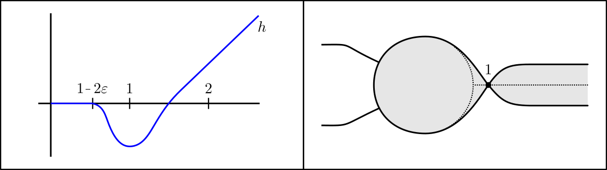
Figure 3. Left: the behaviour of the profile function $h$. Right: the projection to $\mathbb{C}$ of a cobordism after perturbation of a positive end.

Fix a double point of $\iota_{L}$ and pick an ordering $(P_{-},P_{+})$ of the two preimages. Let $D_{\pm}\subset L$ be disjoint open disks centered at $P_{\pm}$. Fix bump functions $\chi_{\pm}$ on $D_{\pm}$ such that $\chi_{\pm}\geq 0$, $\chi\equiv 1$ near $P_{\pm}$ and $\chi\equiv 0$ near $\partial D_{\pm}$. We now define functions $H_{\pm}:[0,\infty)\times D_{\pm}\to\mathbb{R}$ by setting $H_{\pm}(x,p)=\pm h(x)\,\chi_{\pm}(p)$. Doing this for each pair of double points and extending by zero, we obtain a function $H$ on $V$. Finally, extend $H$ to a neighborhood of $V$ in $T^{*}V$ by pulling back by the projection $T^{*}V\to V$.

Consider the family of Lagrangian immersions $\iota_{t}=\Psi\circ\phi^{t}_{H}|_{V}$ for small $t$. By our choice of $h$, for $t>0$ the projection of $\iota_{t}$ to $\mathbb{C}$ has the shape shown in Figure 3. The key feature is that for $t$ small enough each pair of intervals of double points of $\iota_{V}$ inside $[0,\infty)\times L$ has been replaced by two pairs of transverse double points. One of these pairs projects to the "bottleneck" at $x=1$, while the other pair is a small perturbation of the double points $(1-\varepsilon,P_{\pm})$ of $\iota_{V}$.

Assuming that $\iota_{V}$ does not bound teardrops, then by Lemma 4.8, for $t$ small enough $\iota_{t}$ also does not bound teardrops. We will always assume that $t$ is chosen small enough so that this is the case.

In the case of a negative end of $V$, the perturbation is defined in a similar way, with the profile function $h$ replaced by $x\mapsto-h(-x)$.

We now proceed to the proof of Proposition 4.11.

Proof of Proposition 4.11..

We only provide details for the case where $V$ is the concatenation of two cobordisms; the general case is similar.

Let $V$ be the concatenation of topologically unobstructed cobordisms $V_{0}$ and $V_{1}$ along a matching end modelled over the immersed Lagrangian $L$. After generic perturbations, we may assume that $L$ has generic self-intersections and that the only non-generic self-intersections of $V_{0}$ and $V_{1}$ are along the end corresponding to $L$. By Lemma 4.8, for a small enough perturbation the resulting cobordisms are still topologically unobstructed.

Next, perturb $V$ by splicing together compatible perturbations of the ends of $V_{0}$ and $V_{1}$ which were concatenated, as described in the beginning of this section. The outcome is a cobordism (which we still call $V$) with generic self-intersections and two bottlenecks $\zeta_{\pm}\in\mathbb{C}$ as in Figure 4. The bottlenecks separate the cobordism in three parts which we label $V_{\ell}$, $V_{c}$ and $V_{r}$. Note that $V_{\ell}$, $V_{r}$ and $V_{c}$ are topologically unobstructed since they are small perturbations of $V_{0}$, $V_{1}$ and a product cobordism $I\times L$, respectively.

Figure 4. The projection to $\mathbb{C}$ of the cobordism obtained by perturbing the concatenation of $V_{0}$ and $V_{1}$.

Let $J$ be a compatible almost complex structure on $\mathbb{C}\times M$ with the following properties:

1. The projection $\pi_{\mathbb{C}}$ is $(J,i)$-holomorphic outside $K\times M$ for some compact set $K\subset\mathbb{C}$.

2. The projection $\pi_{\mathbb{C}}$ is $(J,i)$-holomorphic on $U_{\pm}\times M$, where $U_{\pm}$ is a neighborhood of the bottleneck $\zeta_{\pm}$.

We claim that $(V,J)$ is quasi-exact. Indeed, if there is a $J$-holomorphic teardrop with boundary on $V$, then by the open mapping theorem this teardrop cannot cross the bottlenecks, i.e. it must have boundary on one of the three parts $V_{\ell}$, $V_{c}$ or $V_{r}$. This contradicts that these immersions are topologically unobstructed. By the same argument, $V$ does not bound non-constant $J$-holomorphic disks. ∎

5. Topological obstruction of surgery cobordisms in dimension 2

We now turn to the computation of $\Omega_{\operatorname{unob}}(\Sigma)$ for a closed surface $\Sigma$ of genus $g\geq 2$, which will take up the rest of this paper. As a first step, in this section we prove topological unobstructedness results for the cobordisms associated to the surgery of immersed curves in $\Sigma$. These results will form the basis of the proofs that the cobordisms appearing in the computation of $\Omega_{\operatorname{unob}}(\Sigma)$ are unobstructed. We note that the proofs in this section make heavy use of special features of the topology of surfaces.

Throughout this section, we fix immersed curves $\alpha$ and $\beta$ in $\Sigma$ that are in general position and intersect at a point $s\in\Sigma$. In Section 5.1, we give a precise description of the Lagrangian surgery of $\alpha$ and $\beta$ at $s$ and of the associated surgery cobordism, which we denote $S(\alpha,\beta;s)$. In Section 5.2 we consider teardrops with boundary $S(\alpha,\beta;s)$, and in Section 5.3 we characterize the existence of non-trivial disks with boundary on $S(\alpha,\beta;s)$.

5.1. Construction of the surgery cobordism

We recall the construction of the surgery cobordism $S(\alpha,\beta;s)$ in order to fix notations for the proofs of the obstruction results of the next sections. We closely follow the construction given by Biran and Cornea [BC13, Section 6.1], although our presentation differs slightly since we will need some control over the double points of the surgery cobordism in order to investigate teardrops.

We start with a local model, which is the surgery of the Lagrangian subspaces $\mathbb{R}$ and $i\mathbb{R}$ in $\mathbb{C}$. Fix an embedding $c:\mathbb{R}\to\mathbb{C}$ with the following properties. Writing $c=c_{1}+ic_{2}$, we have for some $\varepsilon>0$

• $c(t)=t$ for $t\leq-\frac{\varepsilon}{2}$ and $c(t)=it$ for $t\geq\frac{\varepsilon}{2}$,

• $c_{1}^{\prime}(t)>0$ and $c_{2}^{\prime}(t)>0$ for $t\in(-\frac{\varepsilon}{2},\frac{\varepsilon}{2})$,

• $c_{1}^{\prime\prime}(t)<0$ and $c_{2}^{\prime\prime}(t)>0$ for $t\in(-\frac{\varepsilon}{2},\frac{\varepsilon}{2})$.

The local model for the surgery is then the Lagrangian $\mathbb{R}\#i\mathbb{R}=c(\mathbb{R})\cup-c(\mathbb{R})$.

To define the local model for the surgery cobordism, consider the Lagrangian embedding

$$\psi:\mathbb{R}\times S^{1} \longrightarrow\mathbb{C}^{2}$$

$$(t,(x,y)) \longmapsto(c(t)x,c(t)y).$$

The model for the surgery cobordism is the Lagrangian $1$-handle $\psi(W)$, where

$$W=\{(t,(x,y)):x\geq 0,|tx|\leq\varepsilon\}.$$ (7)

Note that $\psi(W)$ is a submanifold of $\mathbb{C}^{2}$ with boundary $(\{-\varepsilon\}\times\mathbb{R})\cup(\{i\varepsilon\}\times i\mathbb{R})\cup(\{0\}\times\mathbb{R}\#i\mathbb{R})$.

Suppose now that $\alpha$ and $\beta$ are immersed curves in $\Sigma$ in general position. Let $s$ be a positive intersection for the pair $(\alpha,\beta)$. Let $B(0,\varepsilon)$ be the open disk of radius $\varepsilon$ in $\mathbb{C}$. For a small enough $\varepsilon>0$, fix a Darboux chart $\Phi:B(0,\varepsilon)\to U\subset\Sigma$ centered at $s$ with the property that $\Phi^{-1}\circ\alpha$ parametrizes $\mathbb{R}$ in the positive direction and $\Phi^{-1}\circ\beta$ parametrizes $i\mathbb{R}$. The surgery $\alpha\#_{s}\beta$ is defined by taking the union $\alpha\cup\beta$ and replacing its intersection with $U$ by the local model $\mathbb{R}\#i\mathbb{R}$. Note that the resulting immersion is independent of the above choices up to Hamiltonian isotopy. Moreover, since $s$ is positive the surgery has a canonical orientation which is compatible with those of $\alpha$ and $\beta$.

To construct the surgery cobordism, start with the product cobordisms $\widehat{\alpha}=[-1,0]\times\alpha$ and $\widehat{\beta}=i[0,1]\times\beta$. These cobordisms are oriented so that $[-1,0]$ is oriented from $-1$ to $0$, and $i[0,1]$ is oriented from $i$ to $0$. Let $\widehat{\iota}:S\to\mathbb{C}\times\Sigma$ be the Lagrangian immersion obtained from $\alpha\cup\beta$ by removing its intersection with $B(0,\varepsilon)\times U$ and gluing the handle $\psi(W)$ using the Darboux chart $\operatorname{id}\times\Phi:B(0,\varepsilon)\times B(0,\varepsilon)\to B(0,\varepsilon)\times U$. Then $\widehat{\iota}$ is a Lagrangian immersion of a pair of pants whose restriction to the boundary coincides with the immersions $\{-1\}\times\alpha$, $\{i\}\times\beta$ and $\{0\}\times(\alpha\#_{s}\beta)$. Note that the handle $\psi(W)$ is compatible with the orientations of $\widehat{\alpha}$ and $\widehat{\beta}$, so that $S$ is canonically oriented.

The immersion $\widehat{\iota}$ is almost the required cobordism $\alpha\#_{s}\beta\rightsquigarrow(\alpha,\beta)$, except that it is not cylindrical near the boundary component that projects to $0\in\mathbb{C}$. We perturb $\widehat{\iota}$ to make it cylindrical using the argument of [BC13, Section 6.1].

To describe the perturbation, we first introduce some notations. Write

$$P=S-\widehat{\iota}^{-1}(B(0,\varepsilon)\times U),$$

so that $\widehat{\iota}$ coincides over $P$ with restrictions of the products $\widehat{\alpha}$ and $\widehat{\beta}$. Let $C$ be the boundary component of $S$ that projects to $0\in\mathbb{C}$. Let $\mathcal{U}$ be a collar neighborhood of $C$. Taking $\mathcal{U}$ smaller if necessary, assume that there is an isomorphism $\mathcal{U}\cong(-\delta,0]\times S^{1}$ that extends the obvious identification over $P$.

Extend the immersion $\widehat{\iota}:S\to\mathbb{C}\times\Sigma$ to a symplectic immersion $\varphi:\mathcal{N}\to\mathbb{C}\times\Sigma$, where $\mathcal{N}$ is a convex neighborhood of the zero-section in $T^{*}S$. We make the following assumptions on $\varphi$. First, taking $\mathcal{N}$ smaller if necessary, we may assume that $\varphi$ is an embedding on each fiber and that $\varphi$ does not have self-intersections that project to the subset $\widehat{\iota}^{-1}(\mathbb{C}\times\overline{U})$. Secondly, we choose $\varphi$ so that over $P$ it is compatible with the splitting of $\widehat{\iota}$ into a product.

Write $\gamma=\alpha\#_{s}\beta$ and consider the immersed Lagrangian submanifold $I\times\gamma$, where $I=\{x+iy\in\mathbb{C}:y=-x\}$. Taking $\mathcal{U}$ smaller if necessary, we may assume that $\varphi^{-1}(I\times\gamma)$ is the graph of a closed $1$-form $\eta$ on $\mathcal{U}$ that vanishes on $C$. Since $\mathcal{U}$ deformation retracts onto $C$, $\eta$ is exact. Write $\eta=dG$ for a function $G$ on $\mathcal{U}$. Let $r$ be the collar coordinate on $\mathcal{U}$ and let $\chi(r)$ be an increasing smooth function such that $\chi(r)=0$ near $-\delta$ and $\chi(r)=1$ on a neighborhood of $0$. Extend the function $\chi(r)G$ to $S$ by $0$. Finally, the desired immersion $\iota:S\to\mathbb{C}\times\Sigma$ is the composition of $\varphi$ with the graph of $d(\chi G)$, which is then isotoped to make its ends horizontal.

Notation.

In the remainder of this section, we will use the following notations to describe $S(\alpha,\beta;s)$. We denote by $S$ the domain of the cobordism and by $\iota:S\to\mathbb{C}\times\Sigma$ the immersion of $S$. We denote by $A$, $B$ and $C$ the boundary components of $S$ which correspond, respectively, to the curves $\alpha$, $\beta$ and $\gamma:=\alpha\#_{s}\beta$. We call $H=\iota^{-1}(\mathbb{C}\times U)$ the handle region, where $U$ is the Darboux chart around $s$ used to define the surgery. We call $K=\iota^{-1}(\mathbb{C}\times\{s\})$ the core of the handle. See Figure 5 for a schematic representation of $S$.

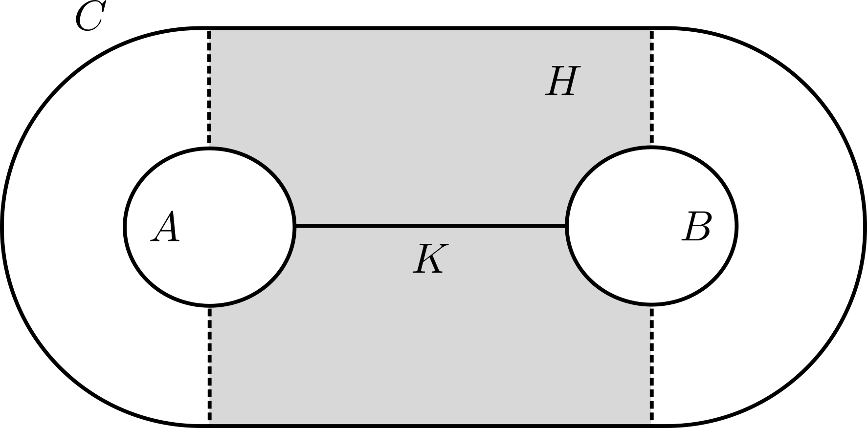
Figure 5. Schematic representation of the domain of a surgery cobordism. The handle $H$ is shaded. On the complement of $H$, the cobordism is equivalent to a product.

The following properties of $S(\alpha,\beta;s)$ are straightforward consequences of the construction.

Lemma 5.1.

The surgery cobordism $S(\alpha,\beta;s)$ satisfies the following properties:

1. All the double points of $\iota$ belong to $S\setminus H$.

2. Over $S\setminus H$, $\iota$ is equivalent to restrictions of the product immersions $\lambda\times\alpha$ and $\lambda^{\prime}\times\beta$, where $\lambda$ and $\lambda^{\prime}$ are embedded paths in $\mathbb{C}$.

Proof.

Property (i) follows from the fact that $H$ does not contain double points of the original immersion $\widehat{\iota}$. Our assumptions about the Weinstein neighborhood $\varphi$ imply that this is still true after perturbation.

Property (ii) follows from the fact that the $\Sigma$ component of $\widehat{\iota}$ agrees with the $\Sigma$ component of $I\times\gamma$ over $P$, and that the Weinstein immersion $\varphi$ is chosen to respect the splitting of $\iota$ into a product over $P$. It follows that over $P$ the $1$-form $\eta$ used to define the perturbation is given by $\eta=f(r)dr$, where $r$ is the collar coordinate on $\mathcal{U}$. This implies that the perturbed immersion has the claimed form over $S\setminus H$. ∎

5.2. Teardrops on surgery cobordisms

By construction, the projection of the surgery cobordism $S(\alpha,\beta;s)$ to $\Sigma$ consists of $\alpha\cup\beta$ and a small neighborhood of $s$. In particular, the projection deformation retracts onto $\alpha\cup\beta$. Therefore, the projection of a polygon with boundary on $S(\alpha,\beta;s)$ should correspond, via this deformation, to a polygon with boundary on $\alpha\cup\beta$ that may have additional corners at $s$. This leads to the following definition.

Definition 5.2.

Let $\alpha$ and $\beta$ be immersed curves intersecting at $s$. A polygon with boundary on $\alpha$ and $\beta$ is called an $s$-marked teardrop if it has one corner at a point $c$ distinct from $s$, and all remaining corners at $s$.

See Figure 6 for some examples of $s$-marked teardrops. Note that in the preceding definition we allow the case where there is no corner at $s$; the polygon is then an ordinary teardrop on one of the curves.

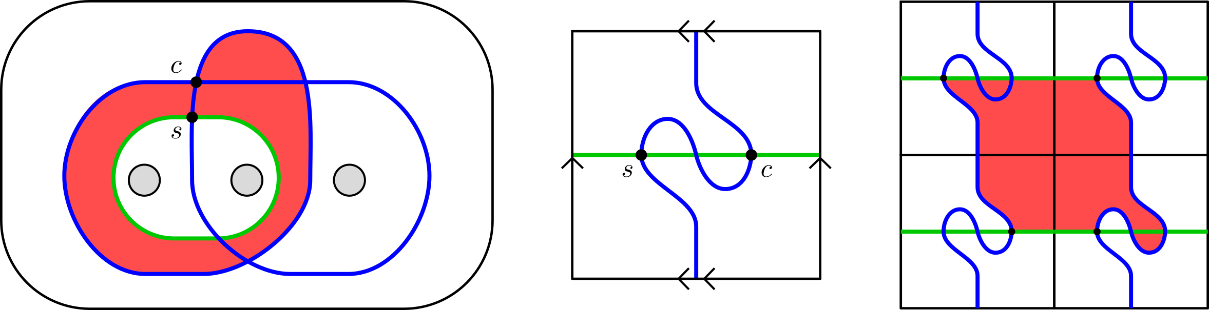
Figure 6. Left: curves on the four-holed sphere that bound an $s$-marked triangle. Center and right: curves on the torus that bound an $s$-marked square, with the square drawn in the universal cover of the torus.

To relate teardrops on $S(\alpha,\beta;s)$ with $s$-marked teardrops on $\alpha\cup\beta$, we will use the following lemma, which makes the above deformation argument precise.

Lemma 5.3.

There is a strong deformation retraction $r:S\times[0,1]\to S$ of $S$ onto $A\cup B\cup K$ that satisfies

$$\pi_{\Sigma}\circ\iota\circ r_{s}(p)=\pi_{\Sigma}\circ\iota(p)$$ (8)

for all $s\in[0,1]$ and for all $p\in S\setminus H$.

Proof.

Recall that the cobordism $\iota$ is obtained by perturbing an immersion $\widehat{\iota}$. Moreover, over $S\setminus H$ we have $\pi_{\Sigma}\circ\iota=\pi_{\Sigma}\circ\widehat{\iota}$. Hence, it suffices to construct the required deformation retraction for $\widehat{\iota}$.

For the immersion $\widehat{\iota}$, the claim follows from a standard argument, using the fact that $\widehat{\iota}$ is obtained from the product cobordisms $\widehat{\alpha}$ and $\widehat{\beta}$ by attaching the index $1$ handle $H$. This can be made precise by the following general argument. Observe that the function $(x+iy,p)\mapsto x-y$ on $\mathbb{C}\times\Sigma$ restricts to a Morse function $f$ on $S$ with a single critical point of index $1$, which lies on $K$. The required deformation retraction can then be obtained by using the negative gradient flow of $f$ away from $K$ and a straight-line homotopy near $K$, as explained in [Mil65, Theorem 3.14]. ∎

The purpose of condition (8) in the previous lemma is to control the behaviour of the double points of $\iota$ throughout the deformation.

Proposition 5.4.

Let $\alpha$ and $\beta$ be immersed curves intersecting at $s$. Then the surgery cobordism $S(\alpha,\beta;s)$ bounds a teardrop if and only if $\alpha$ and $\beta$ bound an $s$-marked teardrop.

Proof.

Suppose first that $S(\alpha,\beta;s)$ bounds a teardrop $u$. We see the boundary lift of $u$ as a path $\delta:[0,1]\to S$ with distinct endpoints and with $\iota(\delta(0))=\iota(\delta(1))$. Since the handle $H$ does not contain double points of $\iota$, the endpoints of $\delta$ lie in $S\setminus H$. By applying the retraction of Lemma 5.3, we obtain a new path $\delta^{\prime}:=r_{1}\circ\delta$ on $A\cup B\cup K$ whose endpoints are distinct and belong to $A\cup B$. By a further homotopy, we can assume that this path is locally embedded. By condition (8) of Lemma 5.3, the path $\lambda:=\pi_{\Sigma}\circ\iota\circ\delta^{\prime}$ is a loop which is homotopic relative endpoints to the loop $\pi_{\Sigma}\circ\iota\circ\delta$. It follows that $\lambda$ is null-homotopic, hence is the boundary of a disk $v$ with boundary on $\alpha\cup\beta$. The disk $v$ is an $s$-marked teardrop; indeed, it has one corner corresponding to projection of the corner of $u$, and the remaining corners at $s$ correspond to the (finitely many) times when $\lambda$ crosses $K$.

Conversely, suppose that $\alpha\cup\beta$ bounds an $s$-marked teardrop $v$ with corner at $c$. Identify $A$ and $B$ with the domains of $\alpha$ and $\beta$, respectively. Then the boundary lifts of $v$ can be seen as paths in $A\cup B$ with endpoints at the preimages of $s$ and $c$. Whenever $v$ has a corner that maps to $s$, the boundary lifts on each side of the corner can be glued together by concatenating them with a path going along the core $K$. Since all the corners of $v$ except one are mapped to $s$, by doing this we obtain a single path $\delta$ in $A\cup B\cup K$ with endpoints on the two preimages of the other corner $c$.

If the endpoints of $\delta$ lie on the same component of $A\cup B$, then $\iota\circ\delta$ is a loop. This loop is null-homotopic in $\mathbb{C}\times\Sigma$ since by construction $\pi_{\Sigma}\circ\iota\circ\delta$ is a reparametrization of $v|_{\partial\mathbb{D}}$. Hence $\iota\circ\delta$ extends to a disk $u:\mathbb{D}\to\mathbb{C}\times\Sigma$ with boundary on $\iota(S)$. This disk is a teardrop since the path $\delta$ is a boundary lift of $u$.

If the endpoints of $\delta$ de not lie on the same component of $A\cup B$, we close up $\iota\circ\delta$ into a loop in the following way. By Lemma 5.3, for each endpoint of $\delta$, there is a path in $(\pi_{\Sigma}\circ\iota)^{-1}(c)$ that connects that endpoint to the boundary component $C$. Concatenating $\delta$ with these paths yields a path $\delta^{\prime}$ with endpoints on $C$ with the property that $\iota\circ\delta^{\prime}$ is a loop. By the same argument as in the previous case, $\delta^{\prime}$ is the boundary lift of a teardrop on $\iota$. ∎

Next, we give a simple algebraic obstruction to representing a class in $\pi_{2}(\Sigma,\alpha\cup\beta,s)$ by an $s$-marked teardrop. Since $\alpha$ and $\beta$ are in general position, we can see the union $\alpha\cup\beta$ as a $4$-valent oriented graph (i.e. a $1$-dimensional CW complex) embedded in $\Sigma$, whose vertices are the intersections and self-intersections of the curves. For each vertex $v$ of this graph, there is an integral cellular $1$-cocycle $\rho_{v}$ supported on the edges incident to $v$, whose values are prescribed by Figure 7. This cocycle can be thought of as giving an algebraic count of the number of corners that a cycle has at $v$.

Figure 7. The definition of the cocycle $\rho_{v}$ that counts the algebraic number of corners of a cycle at $v$.

For a class $A\in\pi_{2}(\Sigma,\alpha\cup\beta,s)$, we denote by $\partial A\in H_{1}(\alpha\cup\beta;\mathbb{Z})$ the image of its boundary by the Hurewicz morphism.

Lemma 5.5.

Suppose that the class $A\in\pi_{2}(\Sigma,\alpha\cup\beta,s)$ can be represented by an $s$-marked teardrop with corner at $c$. Then $\rho_{c}(\partial A)=\pm 1$ and $\rho_{v}(\partial A)=0$ for every vertex $v$ distinct from $c$ and $s$.

Proof.

Suppose that $A$ can be represented by a polygon $u$ that has no corners at the vertex $v$. Let $G$ be the graph obtained by pulling apart the two branches of $\alpha\cup\beta$ meeting at $v$. To be precise, $G$ is obtained from $\alpha\cup\beta$ by adding a vertex $v^{\prime}$ and has the same set of edges, except that the two $\beta$ edges incident to $v$ in $\alpha\cup\beta$ are incident to $v^{\prime}$ in $G$. That $u$ has no corner at $v$ means that $\partial u$ factors through the quotient map $G\to\alpha\cup\beta$ that identifies $v^{\prime}$ and $v$. Since the pullback of $\rho_{v}$ to $G$ is exact, we conclude that $\rho_{v}(\partial A)=0$.

Suppose now that $A$ can be represented by a polygon $u$ that has one corner at the vertex $c$. Let $E$ and $E^{\prime}$ be the edges of $\alpha\cup\beta$ visited by $\partial u$ before and after passing through the corner $c$, and suppose that their endpoints are $\{c,p\}$ and $\{c,q\}$, respectively. Since $\partial u$ has a corner at $c$, one of these edges has $\rho_{c}=\pm 1$, and the other one has $\rho_{c}=0$. The loop $\partial u$ is homotopic to the concatenation of a simple path going from $p$ to $c$ along $E$, a simple path going from $c$ to $q$ along $E^{\prime}$, and a path going from $q$ back to $p$ that has no corners at $c$. Hence $\rho_{c}([\partial u])=\rho_{c}(E)\pm\rho_{c}(E^{\prime})=\pm 1$. ∎

5.3. Disks on surgery cobordisms

As a consequence of Lemma 5.3, we also obtain the following criterion for the existence of non-trivial disks on surgery cobordisms.

Proposition 5.6.

Let $\alpha$ and $\beta$ be immersed curves intersecting at $s$. Then the surgery cobordism $S(\alpha,\beta;s)$ is incompressible if and only if $\alpha$ and $\beta$ span a free group of rank $2$ in $\pi_{1}(\Sigma,s)$.

Proof.

We equip $S$ with the basepoint $x$ which is the intersection of $A$ and $K$. By retracting $S$ onto $A\cup B\cup K$ as in Lemma 5.3 and then collapsing $K$ to a point, we obtain a homotopy equivalence $S\to S^{1}\vee S^{1}$ that makes the following diagram commute up to homotopy:

(9)

Here, $\alpha$ and $\beta$ are seen as loops based at $s$, the wedge sum identifies the two preimages of $s$, and $x_{0}$ is the wedge point.

Since the vertical maps in Diagram (9) are homotopy equivalences, we deduce that $\iota$ is incompressible if and only if the map $\mu:\pi_{1}(S^{1}\vee S^{1},x_{0})\to\pi_{1}(\Sigma,s)$ induced by $\alpha\vee\beta$ is injective.

The image of $\mu$ is the subgroup $\langle[\alpha],[\beta]\rangle$ of $\pi_{1}(\Sigma,s)$ generated by $\alpha$ and $\beta$. Therefore, if $\mu$ is injective then $\langle[\alpha],[\beta]\rangle\cong\pi_{1}(S^{1}\vee S^{1},x_{0})$, which is a free group of rank $2$. Conversely, if $\langle[\alpha],[\beta]\rangle$ is a free group of rank $2$, then $\mu$ maps a free group of rank $2$ onto a free group of rank $2$. Since free groups of finite rank are Hopfian, $\mu$ is an isomorphism on its image. Hence, we conclude that $\mu$ is injective if and only if $\langle[\alpha],[\beta]\rangle$ is a free group of rank $2$. ∎

For a surface of genus $g\geq 2$, the subgroup of $\pi_{1}$ generated by two elements is always free. This is a special case of the following result of Jaco.

Theorem 5.7 ([Jac70, Corollary 2]).

Let $\Sigma$ be a surface with $\chi(\Sigma)\leq 0$. Then any subgroup of $\pi_{1}(\Sigma)$ generated by $k$ elements, where $k<2-\chi(\Sigma)$, is a free group.

In the setting of Proposition 5.6, this implies that the subgroup of $\pi_{1}(\Sigma,s)$ generated by $\alpha$ and $\beta$ is a free group of rank $2$ or less. The rank is $0$ or $1$ if and only if there is some non-trivial relation $[\alpha]^{p}=[\beta]^{q}$ in $\pi_{1}(\Sigma,s)$. Hence we can reformulate Proposition 5.6 as follows.

Proposition 5.8.

Let $\alpha$ and $\beta$ be immersed curves intersecting at $s$. Then the surgery cobordism $S(\alpha,\beta;s)$ is incompressible if and only if there are no integers $p$ and $q$ with $(p,q)\neq(0,0)$ such that $[\alpha]^{p}=[\beta]^{q}$ in $\pi_{1}(\Sigma,s)$.

We will often make use of the following special case of the preceding results.

Corollary 5.9.

Let $\alpha$ and $\beta$ be immersed curves intersecting at $s$. If $\alpha\cdot\beta\neq 0$, then the surgery cobordism $S(\alpha,\beta;s)$ is incompressible.

Proof.

The hypothesis implies that the intersection pairing restricted to $\langle[\alpha],[\beta]\rangle$ is non-trivial. Hence, $\langle[\alpha],[\beta]\rangle$ cannot be a free group of rank $0$ or $1$. By Theorem 5.7, it must be a free group of rank $2$, and the conclusion follows from Proposition 5.6. ∎

6. Lagrangian cobordism invariants of curves

In this section, we define the Lagrangian cobordism invariants of curves on symplectic surfaces that give rise to the morphism

$$\Omega_{\operatorname{unob}}(\Sigma)\to H_{1}(S\Sigma;\mathbb{Z})\oplus\mathbb{R}$$

of Theorem B. These invariants are the same as those considered by Abouzaid [Abo08], who showed that they induce well-defined morphisms on $K_{0}\operatorname{DFuk}(\Sigma)$. Our aim in this section is to show that these invariants also descend to morphisms on $\Omega_{\operatorname{imm}}(\Sigma)$ (and hence on $\Omega_{\operatorname{unob}}(\Sigma)$). Moreover, in Section 6.3, we compute these invariants in some cases which are relevant to the proof of Theorem B.

6.1. Discrete invariants

For a symplectic manifold $M^{2n}$, we write $\mathcal{L}^{\operatorname{or}}(M)$ for the Grassmannian of oriented Lagrangian subspaces of $TM$. This is a fiber bundle with fiber $\Lambda_{n}$, the oriented Lagrangian Grassmannian of $\mathbb{C}^{n}$. Recall that $\Lambda_{n}\cong U(n)/SO(n)$. In the case of a surface $\Sigma$, we identify $\mathcal{L}^{\operatorname{or}}(\Sigma)$ with the unit tangent bundle of $\Sigma$, which we denote $S\Sigma$. We associate to an immersed curve $\gamma:S^{1}\to\Sigma$ the class $[\widetilde{\gamma}]\in H_{1}(S\Sigma;\mathbb{Z})$, where $\widetilde{\gamma}:S^{1}\to S\Sigma$ is the Gauss map of $\gamma$. We will show that this gives rise to a morphism $\Omega_{\operatorname{imm}}(\Sigma)\to H_{1}(S\Sigma;\mathbb{Z})$.

To see this, consider the stabilization map $i:\mathcal{L}^{\operatorname{or}}(\Sigma)\to\mathcal{L}^{\operatorname{or}}(\mathbb{C}\times\Sigma)$ that sends an oriented Lagrangian subspace $U\subset T_{p}\Sigma$ to the Lagrangian subspace $\mathbb{R}\oplus U$ of $T_{(z,p)}(\mathbb{C}\times\Sigma)$, equipped with the product orientation. Here, $z\in\mathbb{C}$ is fixed, but the map does not depend on this choice up to homotopy.

Lemma 6.1.

The stabilization map $i$ induces an isomorphism on $H_{1}(-;\mathbb{Z})$.

Proof.

It suffices to prove that stabilization induces an isomorphism on $\pi_{1}$. To see this, recall that the determinant map $\Lambda_{n}\to S^{1}$ coming from the identification $\Lambda_{n}\cong U(n)/SO(n)$ induces an isomorphism on $\pi_{1}$. The stabilization map $\Lambda_{n}\to\Lambda_{n+1}$ commutes with the determinant, hence it also induces an isomorphism on $\pi_{1}$. The result now follows from comparison of the long exact sequences of homotopy groups associated to the fiber bundles $\mathcal{L}^{\operatorname{or}}(\Sigma)$ and $\mathcal{L}^{\operatorname{or}}(\mathbb{C}\times\Sigma)$. ∎

It follows from Lemma 6.1 that the class $[\widetilde{\gamma}]$ is invariant under Lagrangian cobordisms in the following sense.

Proposition 6.2.

Let $V:(\gamma_{1},\ldots,\gamma_{r})\rightsquigarrow\emptyset$ be an oriented Lagrangian cobordism between immersed curves in $\Sigma$. Let $\widetilde{\gamma}_{1},\ldots,\widetilde{\gamma}_{r}$ be the Gauss maps of the ends of $V$. Then

$$\sum_{k=1}^{r}\;[\widetilde{\gamma}_{k}]=0\qquad\text{in }H_{1}(S\Sigma;\mathbb{Z}).$$

Proof.

The cobordism has a Gauss map $V\to\mathcal{L}^{\operatorname{or}}(\mathbb{C}\times\Sigma)$ which extends the stabilizations of the Gauss maps of its ends. This yields the relation

$$\sum_{k=1}^{r}\;i_{*}[\widetilde{\gamma}_{k}]=0\qquad\text{in }H_{1}(\mathcal{L}^{\operatorname{or}}(\mathbb{C}\times\Sigma);\mathbb{Z}).$$

The conclusion now follows from Lemma 6.1. ∎

It follows from Proposition 6.2 that the homology class of the Gauss map descends to a morphism $\Omega_{\operatorname{imm}}(\Sigma)\to H_{1}(S\Sigma;\mathbb{Z})$.

Since $S\Sigma$ is an oriented circle bundle, its homology can be computed from the Gysin sequence

(10)

where the first map sends $1$ to the class of a fiber and $p:S\Sigma\to\Sigma$ is the projection. This sequence splits since $H_{1}(\Sigma;\mathbb{Z})$ is a free abelian group. It will be useful for us to fix a choice of splitting of (10). A splitting map $\mu:H_{1}(S\Sigma;\mathbb{Z})\to\mathbb{Z}_{\chi(\Sigma)}$ will be called a winding number morphism.

Remark 6.3.

The set of splittings of (10) is a torsor over

$$\operatorname{Hom}(H_{1}(\Sigma;\mathbb{Z}),\mathbb{Z}_{\chi(\Sigma)})\cong H^{1}(\Sigma;\mathbb{Z}_{\chi(\Sigma)}).$$

In the terminology of Seidel [Sei00], they correspond to the $\mathbb{Z}_{2\chi(\Sigma)}$-gradings of $\Sigma$ that factor through the oriented Lagrangian Grassmannian. Winding numbers of curves on closed surfaces first appeared in the works of Reinhart [Rei60] and Chillingworth [Chi72].

6.2. Holonomy

We recall the definition of the holonomy of an immersed curve in a surface of genus $g\neq 0$, following [Abo08]. First, fix a primitive $\lambda$ of $p^{*}\omega$, where as before $p:S\Sigma\to\Sigma$ denotes the projection of the unit tangent bundle. Such a primitive exists whenever $\chi(\Sigma)\neq 0$ (see Corollary A.3 for a proof of a more general claim). The holonomy of an immersed curve $\gamma$ is then defined as

$$\operatorname{Hol}_{\lambda}(\gamma):=\int_{S^{1}}\widetilde{\gamma}^{*}\lambda,$$

where $\widetilde{\gamma}$ is the lift of $\gamma$ to $S\Sigma$.

The holonomy of curves admits a straightforward generalization to a class of real-valued cobordism invariants of Lagrangian immersions in monotone symplectic manifolds. For the benefit of the reader, this theory is developed in Appendix A. As in the case of surfaces, the basic observation that leads to these invariants is that for a monotone manifold $M$ the form $p^{*}\omega$ is exact, where $p:\mathcal{L}M\to M$ is the Lagrangian Grassmannian bundle (see Corollary A.3). As a special case of the general theory developed in Appendix A, we prove that holonomy is invariant under oriented Lagrangian cobordisms. The precise statement is as follows.

Proposition 6.4.

Suppose that there is an oriented Lagrangian cobordism $(\gamma_{1},\ldots,\gamma_{r})\rightsquigarrow\emptyset$. Then

$$\sum_{k=1}^{r}\;\operatorname{Hol}_{\lambda}(\gamma_{k})=0.$$

Proof.

This is a special case of Corollary A.10. ∎

By Proposition 6.4, holonomy descends to a morphism $\operatorname{Hol}_{\lambda}:\Omega_{\operatorname{imm}}(\Sigma)\to\mathbb{R}$. From now on, we fix a choice of primitive $\lambda$ and suppress it from the notation.

We will often make use of the following relationship between holonomy and regular homotopies. Recall that a regular homotopy $\phi:S^{1}\times I\to\Sigma$ is a Lagrangian homotopy and therefore has a well-defined flux class $\operatorname{flux}(\phi)\in H^{1}(S^{1};\mathbb{R})$, which by definition is the class that satisfies

$$\operatorname{flux}(\phi)\cdot[S^{1}]=\int_{S^{1}\times I}\phi^{*}\omega.$$

Lemma 6.5.

Let $\phi:S^{1}\times I\to\Sigma$ be a regular homotopy from $\alpha$ to $\beta$. Then

$$\operatorname{Hol}(\beta)-\operatorname{Hol}(\alpha)=\int_{S^{1}\times I}\phi^{*}\omega=\operatorname{flux}(\phi)\cdot[S^{1}].$$

Proof.

The regular homotopy $\phi$ lifts to a homotopy from $\widetilde{\alpha}$ to $\widetilde{\beta}$ in $S\Sigma$. The result then follows from the Stokes Theorem. ∎

6.3. Winding and holonomy of bounding curves

In this section, we compute the winding number and holonomy of curves that bound surfaces in $\Sigma$. We start with the following lemma.

Lemma 6.6.

Suppose that $\sigma$ is a positively oriented fiber of $S\Sigma$. Then

$$\int_{\sigma}\lambda=-\frac{\operatorname{area}(\Sigma)}{\chi(\Sigma)}.$$

Proof.

Suppose that $\sigma$ is the fiber over $x$. Let $v$ be a vector field on $\Sigma$ that has a unique zero at $x$. By the Poincaré-Hopf Theorem, the index of this zero is $\chi(\Sigma)$.

Let $D$ be a smoothly embedded closed disk containing $x$. Consider the section $\widetilde{v}:\Sigma\setminus\operatorname{int}D\to S\Sigma$ given by $\widetilde{v}=v/|v|$. By choosing a trivialization of $S\Sigma$ over $D$, we can find a homotopy in $p^{-1}(D)$ from the loop $\widetilde{v}|_{\partial D}$ to the loop $\sigma$ iterated $-\chi(\Sigma)$ times. Moreover, the area of this homotopy with respect to $p^{*}\omega$ is $\operatorname{area}(D)$. Hence, by the Stokes Theorem, we have

$$-\chi(\Sigma)\,\int_{\sigma}\lambda=\int_{\widetilde{v}|_{\partial D}}\lambda+\operatorname{area}(D)=\operatorname{area}(\Sigma\setminus D)+\operatorname{area}(D)=\operatorname{area}(\Sigma).$$

∎

Lemma 6.7.

Suppose that the curves $\gamma_{k}$, $k=1,\ldots,r$, form the oriented boundary of a compact surface $P\subset\Sigma$. Then,

$$\sum_{k=1}^{r}\operatorname{Hol}(\gamma_{k})=\operatorname{area}(P)-\frac{\chi(P)}{\chi(\Sigma)}\,\operatorname{area}(\Sigma),$$

$$\sum_{k=1}^{r}\mu(\gamma_{k})=\chi(P)\mod\chi(\Sigma).$$

Proof.

Let $v$ be a vector field on $P$ that agrees with the derivatives $\gamma_{k}^{\prime}$ over $\partial P$ and has a unique zero at a point $x\in\operatorname{int}P$. By the Poincaré-Hopf Theorem, the index of $v$ at $x$ is $\chi(P)$.

Let $\sigma$ be the fiber of $S\Sigma$ over $x$, with the positive orientation. Arguing as in the proof of Lemma 6.6, the chain $\sum_{k}\widetilde{\gamma}_{k}-\chi(P)\sigma$ is the boundary of a surface whose area with respect to $p^{*}\omega$ equals $\operatorname{area}(P)$. As a consequence, using Lemma 6.6 we obtain

$$\sum_{k=1}^{r}\operatorname{Hol}(\gamma_{k})=\operatorname{area}(P)+\chi(P)\,\int_{\sigma}\lambda=\operatorname{area}(P)-\frac{\chi(P)}{\chi(\Sigma)}\operatorname{area}(\Sigma).$$

Likewise, since $\mu(\sigma)=1$ by definition, we have

$$\sum_{k=1}^{r}\mu(\gamma_{k})=\chi(P)\,\mu(\sigma)=\chi(P).$$

∎

As a consequence, we obtain the following

Corollary 6.8.

The morphism $\Omega_{\operatorname{unob}}(\Sigma)\to H_{1}(S\Sigma;\mathbb{Z})$ is surjective.

7. Relations between isotopic curves

In this section, we describe how isotopic curves are related in $\Omega_{\operatorname{unob}}(\Sigma)$. We let $\mathcal{I}$ be the subgroup of $\Omega_{\operatorname{unob}}(\Sigma)$ generated by all the elements of the form $[\widetilde{\alpha}]-[\alpha]$, where $\widetilde{\alpha}$ and $\alpha$ are isotopic curves. The main result of this section is the following computation of $\mathcal{I}$.

Proposition 7.1.

The holonomy morphism restricts to an isomorphism $\mathcal{I}\cong\mathbb{R}$.

As an immediate consequence, we deduce that

$$\Omega_{\operatorname{unob}}(\Sigma)\cong\mathbb{R}\oplus\Omega_{\operatorname{unob}}(\Sigma)/\mathcal{I}.$$

Therefore, the computation of $\Omega_{\operatorname{unob}}(\Sigma)$ reduces to the computation of the quotient $\Omega_{\operatorname{unob}}(\Sigma)/\mathcal{I}$.

Definition 7.2.

The quotient

$$\widetilde{\Omega}_{\operatorname{unob}}(\Sigma)=\Omega_{\operatorname{unob}}(\Sigma)/\mathcal{I}$$

is called the reduced unobstructed cobordism group of $\Sigma$.

We emphasize that, by definition, isotopic curves become equal in $\widetilde{\Omega}_{\operatorname{unob}}(\Sigma)$. This will play a crucial role in the proofs of Section 8 and Section 9 by allowing us to put curves in minimal position by isotopies.

7.1. Holonomy and Hamiltonian isotopies

As a first step towards the proof of Proposition 7.1, we show that holonomy completely determines whether two isotopic curves are Hamiltonian isotopic.

Lemma 7.3.

Let $\alpha$ and $\beta$ be isotopic simple curves with $\operatorname{Hol}(\alpha)=\operatorname{Hol}(\beta)$. Then $\alpha$ and $\beta$ are Hamiltonian isotopic.

Proof.

Suppose first that the curves are non-separating. By Lemma 6.5, the holonomy condition implies that any isotopy from $\alpha$ to $\beta$ has zero flux. Moreover, since the curves are non-separating, they induce surjective maps $H^{1}(\Sigma;\mathbb{R})\to H^{1}(S^{1};\mathbb{R})$. By a standard argument, this condition implies that an isotopy from $\alpha$ to $\beta$ extends to an ambient symplectic isotopy with zero flux; see Lemma 6.6 of [Sol13] for a detailed proof. The result now follows from the well-known fact that a symplectic isotopy with zero flux is homotopic relative to its endpoints to a Hamiltonian isotopy; see Theorem 10.2.5 of [MS17].

Suppose now that the curves are separating. Then, by Lemma 6.7, the surfaces bounded by the curves have the same area. The conclusion then follows from a standard Moser isotopy argument. In the case of contractible curves, a detailed proof is given in [AS01, Appendix A]. The same proof applies to the case of separating curves; for completeness, we sketch the argument from [AS01].

Choose a diffeomorphism $\phi$ isotopic to the identity such that $\phi(\alpha)=\beta$. Let $S$ and $S^{\prime}$ be the surfaces bounded by $\alpha$ and $\beta$, respectively. Then $\phi(S)=S^{\prime}$, hence

$$\int_{S}\phi^{*}\omega=\int_{S^{\prime}}\omega=\int_{S}\omega$$

since $S$ and $S^{\prime}$ have the same area. By a Moser isotopy argument (see [AS01, Lemma A.3]), we can find an isotopy $\psi_{t}$ such that $\psi_{1}^{*}(\phi^{*}\omega)=\omega$ and $\psi_{t}(S)=S$. Then the composition $\theta=\phi\circ\psi_{1}$ is symplectic, isotopic to the identity and satisfies $\theta(S)=S^{\prime}$. It follows again from Moser isotopy that the inclusion $\operatorname{Symp}(\Sigma)\hookrightarrow\operatorname{Diff}^{+}(\Sigma)$ is an isomorphism on $\pi_{0}$, hence there is a path $(\theta_{t})$ in $\operatorname{Symp}(\Sigma)$ with $\theta_{0}=\operatorname{id}$ and $\theta_{1}=\theta$. The restriction of $(\theta_{t})$ to $\alpha$ is an exact Lagrangian path, hence $\alpha$ and $\beta$ are Hamiltonian isotopic. ∎

For future use, we also record a version of Lemma 7.3 that applies to topologically unobstructed curves.

Lemma 7.4.

Let $\alpha$ and $\beta$ be homotopic topologically unobstructed curves with $\operatorname{Hol}(\alpha)=\operatorname{Hol}(\beta)$. Then there is an exact homotopy $(\gamma_{t})_{t\in[0,1]}$ such that $\gamma_{0}=\alpha$, $\gamma_{1}=\beta$ and each curve $\gamma_{t}$ is topologically unobstructed.

Proof.

Consider the covering map $\rho:\widehat{\Sigma}\to\Sigma$ associated to the subgroup of $\pi_{1}(\Sigma,\alpha(0))$ generated by $[\alpha]$. Equip $\widehat{\Sigma}$ with the symplectic form $\rho^{*}\omega$.

By definition, $\alpha$ lifts to a closed curve $\widehat{\alpha}$ in $\widehat{\Sigma}$. Moreover, a homotopy from $\alpha$ to $\beta$ lifts to a homotopy from $\widehat{\alpha}$ to a closed curve $\widehat{\beta}$ which is a lift of $\beta$. Since $\alpha$ and $\beta$ are unobstructed, by Lemma 4.6 their lifts to the universal cover of $\Sigma$ are embedded. This implies that $\widehat{\alpha}$ and $\widehat{\beta}$ are simple curves.

Since $\widehat{\alpha}$ and $\widehat{\beta}$ are homotopic non-contractible simple curves, they are isotopic by Theorem 2.1 of [Eps66]. Any isotopy between them has zero flux since its projection to $\Sigma$ is a regular homotopy from $\alpha$ to $\beta$, and this homotopy has zero flux by the holonomy assumption and Lemma 6.5. Moreover, $\widehat{\alpha}$ represents a generator of $\pi_{1}(\widehat{\Sigma})\cong\mathbb{Z}$, hence the map $H^{1}(\widehat{\Sigma};\mathbb{R})\to H^{1}(S^{1};\mathbb{R})$ induced by $\widehat{\alpha}$ is an isomorphism. As in the first case of the proof of Lemma 7.3, it follows that $\widehat{\alpha}$ and $\widehat{\beta}$ are Hamiltonian isotopic. The projection of a Hamiltonian isotopy from $\widehat{\alpha}$ to $\widehat{\beta}$ yields an exact homotopy from $\alpha$ to $\beta$ through unobstructed curves. ∎

7.2. Proof of Proposition 7.1

In this section, we prove Proposition 7.1. First, we show that $\operatorname{Hol}|_{\mathcal{I}}$ is surjective, which is a consequence of the following lemma.

Lemma 7.5.

Let $\alpha$ be a non-separating simple curve. Then for any $x\in\mathbb{R}$, there exists a simple curve $\widetilde{\alpha}$ isotopic to $\alpha$ such that $\operatorname{Hol}(\widetilde{\alpha})-\operatorname{Hol}(\alpha)=x.$

Proof.

There is a curve $\beta$ that intersects $\alpha$ transversely in a single point. Let $A\cong S^{1}\times[0,1]$ be a small tubular neighborhood of $\beta$ such that $\alpha\cap A$ is a ray of the annulus. Then, the required curve $\widetilde{\alpha}$ can be obtained by wrapping $\alpha$ around the annulus by the flow of a vector field of the form $f(r)\frac{\partial}{\partial\theta}$, where $f(r)\geq 0$ is a non-constant function that vanishes near $r=0$ and $r=1$. ∎

It remains to prove that $\operatorname{Hol}|_{\mathcal{I}}$ is injective, which is the hardest part of the proof. We will deduce it from the following proposition, which is a generalization of Lemma 7.3.

Proposition 7.6.

Suppose that $(\alpha,\widetilde{\alpha})$ and $(\beta,\widetilde{\beta})$ are two pairs of isotopic simple curves with $\operatorname{Hol}(\widetilde{\alpha})-\operatorname{Hol}(\alpha)=\operatorname{Hol}(\widetilde{\beta})-\operatorname{Hol}(\beta)$. Then, in $\Omega_{\operatorname{unob}}(\Sigma)$ we have

$$[\widetilde{\alpha}]-[\alpha]=[\widetilde{\beta}]-[\beta].$$

This result appears as Proposition 5.4 and Lemma 5.15 in [Per19]. As explained in Remark 3.5, the extension of Perrier’s result to the present case requires additional verifications to show unobstructedness of the relevant cobordisms. These verifications are straightforward applications of the obstruction criteria proved in Section 4 and Section 5. For the benefit of the reader, we include in Appendix B a proof of Proposition 7.6 that closely follows the proof in [Per19] and incorporates these verifications.

Using Proposition 7.6, we can now finish the proof of Proposition 7.1.

Proof of Proposition 7.1..

By Lemma 7.5, $\operatorname{Hol}|_{\mathcal{I}}$ is surjective. To prove injectivity, we claim that any element of $\mathcal{I}$ can be written as $[\widetilde{\alpha}]-[\alpha]$ for some isotopic curves $\widetilde{\alpha}$ and $\alpha$ (in other words, the subset of elements of the form $[\widetilde{\alpha}]-[\alpha]$ is already a subgroup). Indeed, a general element of $\mathcal{I}$ can be written as a sum $\sum_{k=1}^{N}[\widetilde{\beta}_{k}]-[\beta_{k}]$, where $\widetilde{\beta}_{k}$ and $\beta_{k}$ are isotopic. Fix a non-separating curve $\alpha_{0}$. By Lemma 7.5, we can find curves $\alpha_{k}$ for $k=1,\ldots,N$, such that $\alpha_{k}$ is obtained from $\alpha_{k-1}$ by an isotopy of area $\operatorname{Hol}(\widetilde{\beta}_{k})-\operatorname{Hol}(\beta_{k})$. Then, by Proposition 7.6, we have

$$\sum_{k=1}^{N}[\widetilde{\beta}_{k}]-[\beta_{k}]=\sum_{k=1}^{N}[\alpha_{k}]-[\alpha_{k-1}]=[\alpha_{N}]-[\alpha_{0}].$$

This proves the claim. The injectivity of $\operatorname{Hol}|_{\mathcal{I}}$ now follows directly from Proposition 7.6. ∎

8. Action of the mapping class group

In Section 7, we showed how to reduce the computation of $\Omega_{\operatorname{unob}}(\Sigma)$ to the computation of the reduced cobordism group $\widetilde{\Omega}_{\operatorname{unob}}(\Sigma)$ (see Definition 7.2). The action of the group of symplectic diffeomorphisms $\operatorname{Symp}(\Sigma)$ on $\Omega_{\operatorname{unob}}(\Sigma)$ descends to an action on $\widetilde{\Omega}_{\operatorname{unob}}(\Sigma)$. By definition, the component of the identity $\operatorname{Symp}_{0}(\Sigma)\subset\operatorname{Symp}(\Sigma)$ acts trivially on $\widetilde{\Omega}_{\operatorname{unob}}(\Sigma)$. Therefore, the action of $\operatorname{Symp}(\Sigma)$ descends to an action of the symplectic mapping class group $\operatorname{Mod}_{\omega}(\Sigma)=\operatorname{Symp}(\Sigma)/\operatorname{Symp}_{0}(\Sigma)$ on $\widetilde{\Omega}_{\operatorname{unob}}(\Sigma)$. The goal of this section is to describe this action. This will be a key ingredient in the computation of $\widetilde{\Omega}_{\operatorname{unob}}(\Sigma)$, as it will allow us to determine a simple set of generators of this group (see Proposition 9.2).

The main result of this section is the computation of the action of symplectic Dehn twists, which are generators of $\operatorname{Mod}_{\omega}(\Sigma)$. For a simple curve $\alpha$, we denote by $T_{\alpha}\in\operatorname{Mod}_{\omega}(\Sigma)$ the Dehn twist around $\alpha$ (the definition of $T_{\alpha}$ is recalled in Section 8.1).

Theorem 8.1.

Let $\alpha$ and $\beta$ be two simple curves in $\Sigma$. Then in $\widetilde{\Omega}_{\operatorname{unob}}(\Sigma)$ there is the relation

$$T_{\alpha}[\beta]=[\beta]+(\alpha\cdot\beta)[\alpha].$$ (11)

Theorem 8.1 is proved in two steps. The first step is to prove the theorem in the special case where the curves intersect twice with zero algebraic intersection. This is carried out in Section 8.2. Then, in Section 8.3, we show how to deduce the general case of Theorem 8.1 from the special case by an inductive argument.

Remark 8.2.

On the side of $K_{0}\operatorname{DFuk}$, the existence of the Dehn twist relation (11) is a consequence of the well-known Seidel exact triangle in $\operatorname{DFuk}$

(12)

where $T_{S}$ is the Dehn twist around a framed Lagrangian sphere $S$; see [Sei08, Corollary 17.18]. See also [Abo08] for the existence of the triangle (12) in the case of curves on surfaces that intersect minimally. We remark that the methods used in the present work do not recover the exact triangle (12) on the level of $\operatorname{DFuk}$, but only the induced relation in $K$-theory.

8.1. Dehn twists

We recall the definition of the Dehn twist $T_{\alpha}$ around a simple curve $\alpha$. Choose a symplectic embedding $\psi:[-\delta,\delta]\times S^{1}\to\Sigma$ such that $\psi|_{\{0\}\times S^{1}}=\alpha$, where the annulus is equipped with the standard symplectic form $dt\wedge d\theta$. Consider the symplectic diffeomorphism of the annulus given by

$$(t,\theta)\longmapsto(t,\theta-f(t)),$$

where $f:[-\delta,\delta]\to\mathbb{R}$ is a smooth increasing function which is $0$ near $-\delta$ and $1$ near $\delta$. Using the embedding $\psi$, this map extends by the identity to a symplectomorphism $T_{\alpha}$ of $\Sigma$, called a (right-handed) symplectic Dehn twist around $\alpha$. The class of this map in $\operatorname{Mod}_{\omega}(\Sigma)$ does not depend on the choices of $\psi$ and $f$ above. We will also denote this class by the symbol $T_{\alpha}$, whenever no confusion arises.

Remark 8.3.

We warn the reader that our convention for the direction of the Dehn twist is opposite to that of [Abo08] and [Per19].

By Moser’s Theorem, the inclusion of $\operatorname{Symp}(\Sigma)$ inside the group of orientation-preserving diffeomorphisms $\operatorname{Diff}^{+}(\Sigma)$ induces an isomorphism between $\operatorname{Mod}_{\omega}(\Sigma)$ and the classical mapping class group $\operatorname{Mod}(\Sigma)=\operatorname{Diff}^{+}(\Sigma)/\operatorname{Diff}_{0}(\Sigma)$, where $\operatorname{Diff}_{0}(\Sigma)$ is the subgroup of diffeomorphisms isotopic to the identity. In what follows, we will identify $\operatorname{Mod}_{\omega}(\Sigma)$ and $\operatorname{Mod}(\Sigma)$ using this isomorphism.

It is a well-known theorem of Dehn and Lickorish that $\operatorname{Mod}(\Sigma)$ is generated by the classes of finitely many Dehn twists. It follows that $\operatorname{Mod}_{\omega}(\Sigma)$ is generated by symplectic Dehn twists.

8.2. Proof of Theorem 8.1: curves intersecting twice

In this section, we prove the following special case of Theorem 8.1.

Proposition 8.4.

Let $\alpha$ and $\beta$ be simple curves which are in minimal position and intersect in two points of opposite signs. Then, in $\widetilde{\Omega}_{\operatorname{unob}}(\Sigma)$ we have $T_{\alpha}[\beta]=[\beta]+(\alpha\cdot\beta)[\alpha].$

Proposition 8.4 is proved by realizing the Dehn twist as an iterated surgery. This is a well-known procedure; see for example [FM12, Section 3.1.1]. We will follow the description given by Perrier in [Per19, Proposition 2.15], which we recall in order to fix some notation.

Let $\alpha$ and $\beta$ be curves satisfying the hypothesis of Proposition 8.4. Let $N$ be a closed regular neighborhood of $\alpha\cup\beta$. Note that $N$ is a four-holed sphere. We perform the following surgeries, which are illustrated in Figure 8. Let $s_{1}$ be the positive intersection of $(\alpha,\beta)$, and $q_{1}$ the negative intersection. The first step is to form the surgery $\sigma:=\alpha\#_{s_{1}}\beta$. Next, let $\widetilde{\alpha}$ be a $C^{1}$-small Hamiltonian perturbation of $\alpha^{-1}$ which intersects $\sigma$ in two points. This perturbation is chosen so that one of these intersection points, denoted $s_{2}$, lies on the arc of $\beta$ near $q_{1}$, and the other, denoted $q_{2}$, lies on the arc of $\alpha$ near $q_{1}$. Finally, we let $\tau:=\widetilde{\alpha}\#_{s_{2}}\sigma$. The size of the surgery handle is chosen big enough so that $\tau$ is embedded.

Figure 8. The surgery procedure used in the proof of Proposition 8.4.

It is easy to check that $\tau$ is isotopic to $T_{\alpha}\beta$. We denote the traces of the surgeries by $S_{1}=S(\alpha,\beta;s_{1})$ and $S_{2}=S(\widetilde{\alpha},\sigma;s_{2})$. Concatenating $S_{1}$ and $S_{2}$ produces an immersed cobordism $\tau\rightsquigarrow(\widetilde{\alpha},\alpha,\beta)$. To prove Proposition 8.4, we will show that there is an unobstructed cobordism with the same ends. By Proposition 4.11, it suffices to check that the surgery cobordisms $S_{1}$ and $S_{2}$ constructed above are topologically unobstructed. Hence, to finish the proof of Proposition 8.4, it suffices to show the following lemma.

Lemma 8.5.

Assume that $\alpha$ and $\beta$ are in minimal position. Then the surgery cobordisms $S_{1}$ and $S_{2}$ constructed above are topologically unobstructed.

Before giving the proof of the lemma, we make some preliminary observations. It will be convenient to perform the necessary computations inside the regular neighborhood $N$. To relate computations in $N$ to those in $\Sigma$, we will use the fact that $N$ is incompressible in $\Sigma$ (recall from Definition 4.2 that this means that the maps $\pi_{1}(N)\to\pi_{1}(\Sigma)$ induced by the inclusion are injective).

Lemma 8.6.

Assume that $\alpha$ and $\beta$ are in minimal position. Then the regular neighborhood $N$ of $\alpha\cup\beta$ is incompressible in $\Sigma$.

Proof.

Since the curves $\alpha$ and $\beta$ are in minimal position, it follows from the Bigon Criterion [FM12, Proposition 1.7] that they do not bound bigons. In particular, this implies that the boundary circles of $N$ are non-contractible in $\Sigma$. The incompressibility of $N$ is then a consequence of the following well-known fact.

Lemma 8.7.

Let $M$ be a smooth compact manifold and $X\subset M$ a smooth codimension $0$ compact submanifold with boundary. If $\partial X$ is incompressible in $M$, then $X$ is incompressible in $M$.

We refer to the appendix of [GT23] for an elegant proof of this lemma. In the case of surfaces, $\partial X$ is the union of embedded circles. Since the fundamental group of an orientable surface has no torsion, the condition that $\partial X$ be incompressible is equivalent to the non-contractibility of each component of $\partial X$. Therefore, we conclude from Lemma 8.7 that the regular neighborhood $N$ above is incompressible. ∎

The incompressibility of $N$ implies that for a subset $A\subset N$, the inclusions induce an isomorphism $\pi_{2}(N,A,*)\to\pi_{2}(\Sigma,A,*)$. This follows from comparison of the homotopy exact sequences of the pairs $(N,A)$ and $(\Sigma,A)$.

We now proceed to the proof that the cobordisms $S_{i}$ are topologically unobstructed.

Proof of Lemma 8.5.

$S_{1}$ is topologically unobstructed.

The group $\pi_{1}(N,s_{1})$ is free of rank $3$. The classes $[\alpha]$ and $[\beta]$ belong to a basis of $\pi_{1}(N,s_{1})$, hence span a free group of rank $2$. Since $N$ is incompressible, they also span a free group of rank $2$ in $\pi_{1}(\Sigma,s_{1})$. Hence, by Proposition 5.6, $S_{1}$ is incompressible.

Moreover, we have $\pi_{2}(N,\alpha\cup\beta,s_{1})=0$, hence also $\pi_{2}(\Sigma,\alpha\cup\beta,s_{1})=0$. By Lemma 5.5, $\alpha$ and $\beta$ do not bound $s_{1}$-marked teardrops. We conclude from Proposition 5.4 that $S_{1}$ does not bound teardrops.

$S_{2}$ is topologically unobstructed.

Again, it can be checked directly that $[\widetilde{\alpha}]$ and $[\sigma]$ belong to a basis of $\pi_{1}(N,s_{2})$. By the same argument, it follows that $S_{2}$ is incompressible.

It remains to show that $\widetilde{\alpha}$ and $\sigma$ do not bound $s_{2}$-marked teardrops. The group $\pi_{2}(\Sigma,\widetilde{\alpha}\cup\sigma,s_{2})\cong\pi_{2}(N,\widetilde{\alpha}\cup\sigma,s_{2})$ is isomorphic to $\mathbb{Z}$ and is spanned by the class of the obvious triangle with boundary on $\widetilde{\alpha}\cup\sigma$. Since this triangle has three distinct corners, Lemma 5.5 ensures that no classes in $\pi_{2}(\Sigma,\widetilde{\alpha}\cup\sigma,s_{2})$ can be represented by $s_{2}$-marked teardrops.

∎

8.3. Proof of Theorem 8.1: general case

We now show how to deduce the general case of Theorem 8.1 from the special case of Proposition 8.4. The proof uses an inductive argument based on the following lemma, due to Lickorish.

Lemma 8.8 (Lickorish [Lic64]).

Let $\alpha$ and $\beta$ be simple curves in general position with $N\geq 2$ intersection points. In the case $N=2$, assume that the intersections have the same sign. Then there exists a simple curve $\gamma$ with the following properties:

1. $\gamma$ intersects $\beta$ transversely in one point or two points of opposite signs.

2. $\gamma$ intersects $\alpha$ transversely in at most $N-1$ points.

3. The Dehn twist $T_{\gamma}\beta$ is isotopic to a curve $\delta$ that intersects $\alpha$ transversely in at most $N-1$ points.

Proof.

The idea of the proof is that $\alpha$ and $\beta$ either have

1. two intersections that are consecutive along $\alpha$ and have the same sign, or

2. three intersections that are consecutive along $\alpha$ and have alternating signs.

In each case, a curve $\gamma$ satisfying the above conditions is represented in Figure 9. We refer to the proof of Lemma 2 of [Lic64] for more details.

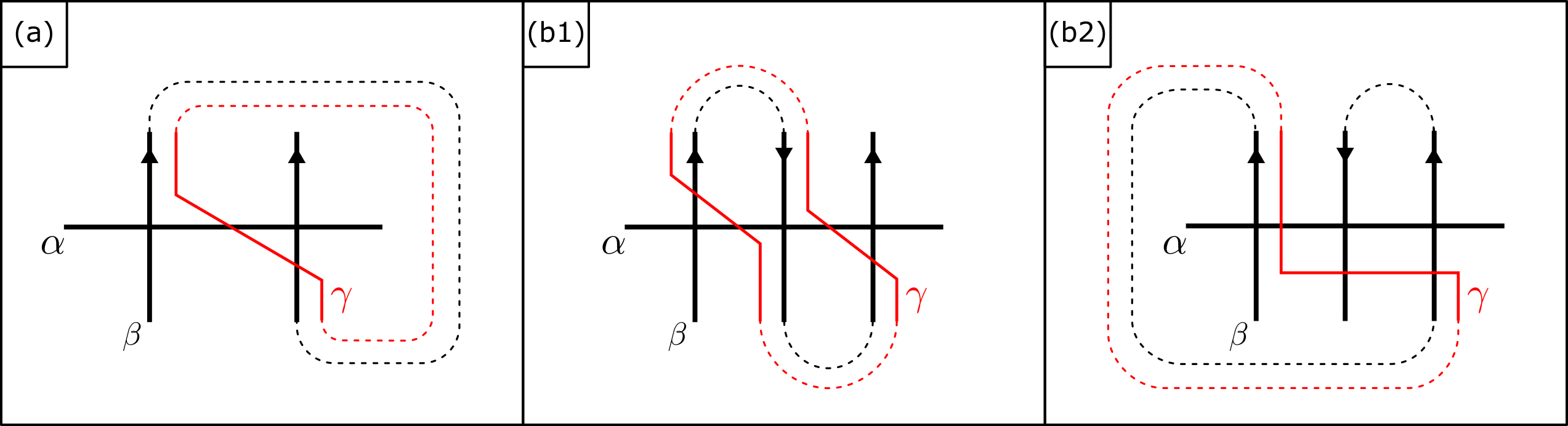
Figure 9. The choice of the curve $\gamma$ in the proof of Lemma 8.8.

∎

Proof of Theorem 8.1..

The proof is by induction over the geometric intersection number $N$ of the curves. By moving $\alpha$ and $\beta$ by isotopies if necessary, we may assume that they are in minimal position.

We start by handling a few base cases. For $N=0$, Formula (11) follows from the fact that $T_{\alpha}\beta$ is isotopic to $\beta$.

For $N=1$, Formula (11) follows from the fact that, in this case, the Dehn twist $T_{\alpha}\beta$ is isotopic either to the surgery $\alpha\#\beta$ if $\alpha\cdot\beta>0$, or to the surgery $\alpha^{-1}\#\beta$ if $\alpha\cdot\beta<0$. The resulting surgery cobordism is embedded and therefore bounds no teardrops. Moreover, it follows from Corollary 5.9 that the cobordism is incompressible. Hence, the surgery cobordism is topologically unobstructed, and therefore unobstructed.

In the case where $N=2$ and $\alpha\cdot\beta=0$, the theorem reduces to Proposition 8.4.

We deal with the remaining cases by induction, using Lemma 8.8 to introduce auxiliary curves whose role is to reduce the number of intersections. Suppose then that $\alpha$ and $\beta$ have geometric intersection number $N\geq 2$, and in the case $N=2$ that $\alpha\cdot\beta\neq 0$. As above, we assume that $\alpha$ and $\beta$ are in minimal position. Let $\gamma$ and $\delta$ be curves satisfying the conclusion of Lemma 8.8.

We claim that $\delta$ and $\gamma$ are non-contractible. Indeed, the curve $\delta$ is isotopic to $T_{\gamma}\beta$, which is non-contractible since $\beta$ is non-contractible. To see that $\gamma$ is non-contractible, note that the geometric intersection number of $T_{\gamma}\beta$ and $\alpha$ is at most $N-1$, which implies that $T_{\gamma}\beta$ is not isotopic to $\beta$. In turn, this implies that $T_{\gamma}$ is not isotopic to the identity, hence that $\gamma$ is non-contractible.

Using the $N=1$ and $N=2$ cases proven before, we have $[T_{\gamma}\beta]=[\beta]+(\gamma\cdot\beta)[\gamma]$. Since $T_{\gamma}\beta$ is isotopic to $\delta$, this gives the relation

$$[\delta]=[\beta]+(\gamma\cdot\beta)[\gamma].$$ (13)

Applying the Dehn twist along $\alpha$, we then obtain:

$$T_{\alpha}[\beta]=T_{\alpha}[\delta]-(\gamma\cdot\beta)T_{\alpha}[\gamma].$$

Since $\alpha$ intersects $\delta$ and $\gamma$ in less than $N$ points, we can use the induction hypothesis and deduce that

$$T_{\alpha}[\beta]=[\delta]+(\alpha\cdot\delta)[\alpha]-(\gamma\cdot\beta)\left([\gamma]+(\alpha\cdot\gamma)[\alpha]\right).$$

Using relation (13) again, this last equality simplifies to $T_{\alpha}[\beta]=[\beta]+(\alpha\cdot\beta)[\alpha]$. ∎

9. Computation of $\Omega_{\operatorname{unob}}(\Sigma)$

In this section, we combine the results of Sections 5 – 8 to complete the computation of the cobordism group $\Omega_{\operatorname{unob}}(\Sigma)$. We will show that the map

$$\Omega_{\operatorname{unob}}(\Sigma)\to H_{1}(S\Sigma;\mathbb{Z})\oplus\mathbb{R}$$

defined in Section 6 is an isomorphism.

Given the results of Sections 6 – 8, the structure of the proof is identical to the computation of $K_{0}\operatorname{DFuk}(\Sigma)$ in Section 7 and Section 8 of [Abo08]. The only new ingredient that is needed is the verification that the surgeries appearing in Lemma 9.3 below, which corresponds to Lemma 7.6 in [Abo08], give rise to unobstructed cobordisms. In the rest of this section, we recall Abouzaid’s computation and indicate the adjustments needed to deal with obstruction.

Figure 10. The Lickorish generators of $\operatorname{Mod}(\Sigma)$.

9.1. Generators of $\widetilde{\Omega}_{\operatorname{unob}}(\Sigma)$

The first step is to determine a simple set of generators for $\widetilde{\Omega}_{\operatorname{unob}}(\Sigma)$. These generators will be obtained from a set of generators of the mapping class group of $\Sigma$. By a well-known theorem of Lickorish [Lic64], $\operatorname{Mod}(\Sigma)$ is generated by the Dehn twists about the $3g-1$ curves $\alpha_{1},\ldots,\alpha_{g}$, $\beta_{1},\ldots,\beta_{g}$ and $\gamma_{1},\ldots,\gamma_{g-1}$ that are represented in Figure 10.

To describe the generators of $\widetilde{\Omega}_{\operatorname{unob}}(\Sigma)$, we will first need the following lemma.

Lemma 9.1.

Suppose that $\gamma$ and $\gamma^{\prime}$ are the oriented boundaries of diffeomorphic compact surfaces in $\Sigma$. Then $[\gamma]=[\gamma^{\prime}]$ in $\widetilde{\Omega}_{\operatorname{unob}}(\Sigma)$.

Proof.

There is an orientation-preserving diffeomorphism of $\Sigma$ that takes $\gamma$ to $\gamma^{\prime}$. This diffeomorphism can be written as the composition of an ambient isotopy and a sequence of symplectic Dehn twists (see Section 8.1). It follows from the Dehn twist relation (11) that $[\gamma]=[\gamma^{\prime}]$ in $\widetilde{\Omega}_{\operatorname{unob}}(\Sigma)$. ∎

We let $T\in\widetilde{\Omega}_{\operatorname{unob}}(\Sigma)$ be the class represented by curves bounding genus $1$ surfaces in $\Sigma$. This is well-defined by Lemma 9.1. We can now state the main result of this section.

Proposition 9.2.

$\widetilde{\Omega}_{\operatorname{unob}}(\Sigma)$ is generated by $T$ and the Lickorish generators $[\alpha_{i}]$ and $[\beta_{i}]$ for $i=1,\ldots,g$.

The proof of the proposition relies on Lemma 9.3 and Lemma 9.4 below.

Lemma 9.3.

Suppose that the curves $\sigma_{1}$, $\sigma_{2}$ and $\sigma_{3}$ form the oriented boundary of a pair of pants. Moreover, assume that at most one of the three curves is separating. Then, in $\widetilde{\Omega}_{\operatorname{unob}}(\Sigma)$ there is the relation

$$[\sigma_{1}]+[\sigma_{2}]+[\sigma_{3}]=T.$$ (14)

Proof.

The proof uses the same surgeries as the proof of Lemma 7.6 in [Abo08], which we recall for convenience. We need to show that the associated surgery cobordisms are unobstructed. The proof splits in two cases: the case where $\Sigma$ has genus $g\geq 3$ and the case where $\Sigma$ has genus $2$. We consider first the case $g\geq 3$.

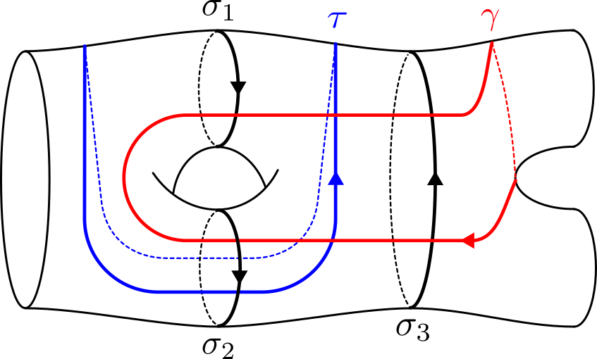
Figure 11. The curves used in the proof of Lemma 9.3 in the case $g\geq 3$.

First, we can assume that none of the curves $\sigma_{i}$ are isotopic to each other. Indeed, if two of the curves are isotopic then the third curve bounds a torus and (14) follows directly from the definition of $T$.

Let $P$ be the pair of pants bounded by the curves $\sigma_{i}$. By assumption, at most one of the curves is separating. Without loss of generality, assume that $\sigma_{1}$ and $\sigma_{2}$ are non-separating. Then there is a curve $\sigma_{4}$ such that $\sigma_{1}$, $\sigma_{2}$ and $\sigma_{4}$ together bound a pair of pants $P^{\prime}$ whose interior is disjoint from $P$.

Let $\tau$ be a curve in $P\cup P^{\prime}$ that bounds a torus $T$ and whose intersection pattern with the $\sigma_{i}$ is specified in Figure 11. We can assume that $\tau$ satisfies the holonomy condition

$$\operatorname{Hol}(\tau)=\operatorname{Hol}(\sigma_{1})+\operatorname{Hol}(\sigma_{2})+\operatorname{Hol}(\sigma_{3}).$$ (15)

Indeed, by Lemma 6.7, this condition is equivalent to $\operatorname{area}(T)=\operatorname{area}(P)$, which can be arranged by an isotopy of $\tau$ without changing the intersection pattern.

Since $\Sigma$ has genus at least $3$, we can find a further curve $\gamma$ which is in minimal position with respect to the curves $\sigma_{i}$ and $\tau$, and whose intersection pattern is specified in Figure 11.

Next, we perform the surgeries represented in Figure 12. In the left column of Figure 12, we perform surgeries between $\sigma_{1}^{-1}$, $\gamma$ and $\tau$, producing a curve $\delta$. In the right column of Figure 12, we perform surgeries between $\gamma$, $\sigma_{2}$ and $\sigma_{3}$, producing a curve $\delta^{\prime}$.

The curves $\delta$ and $\delta^{\prime}$ are topologically unobstructed and regularly homotopic. Moreover, by (15) their holonomies satisfy

$$\operatorname{Hol}(\delta^{\prime})=\operatorname{Hol}(\gamma)+\operatorname{Hol}(\sigma_{2})+\operatorname{Hol}(\sigma_{3})=\operatorname{Hol}(\gamma)+\operatorname{Hol}(\tau)-\operatorname{Hol}(\sigma)=\operatorname{Hol}(\delta).$$

By Lemma 7.4, $\delta$ and $\delta^{\prime}$ are exact homotopic through topologically unobstructed curves. By concatenating the surgery cobordisms obtained above with the suspension of an unobstructed exact homotopy from $\delta$ to $\delta^{\prime}$, we obtain an immersed Lagrangian cobordism $(\sigma_{2},\gamma,\sigma_{3})\rightsquigarrow(\tau,\gamma,\sigma_{1}^{-1})$.

To finish the proof, it remains to show that there is an unobstructed cobordism with the same ends. By Proposition 4.11, it suffices to prove that each step in the above procedure produces a topologically unobstructed cobordism. The surgeries labelled L1 and R1 in Figure 12 involve curves intersecting once, hence they are topologically unobstructed by Corollary 5.9. The surgeries labelled L2 and R2 involve curves which intersect twice. Moreover, these curves are in minimal position since $\gamma$ was chosen to be in minimal position with respect to $\tau$ and $\sigma_{3}$. Hence, we are in the same situation as in Section 8.2, and we conclude that these surgeries are topologically unobstructed by Lemma 8.5. Finally, the exact homotopy between $\delta$ and $\delta^{\prime}$ is topologically unobstructed by Lemma 4.7.

Suppose now that $\Sigma$ has genus $2$. If one of the $\sigma_{i}$ is separating, then it bounds a genus $1$ surface. In this case, the other two curves are isotopic and (14) follows. Suppose now that all the $\sigma_{i}$ are non-separating. Then, up to a diffeomorphism, we are in the situation of Figure 13. To obtain Equation (14), apply the same surgery procedure as above using the curves $\tau$ and $\gamma$ indicated on the right of Figure 13.

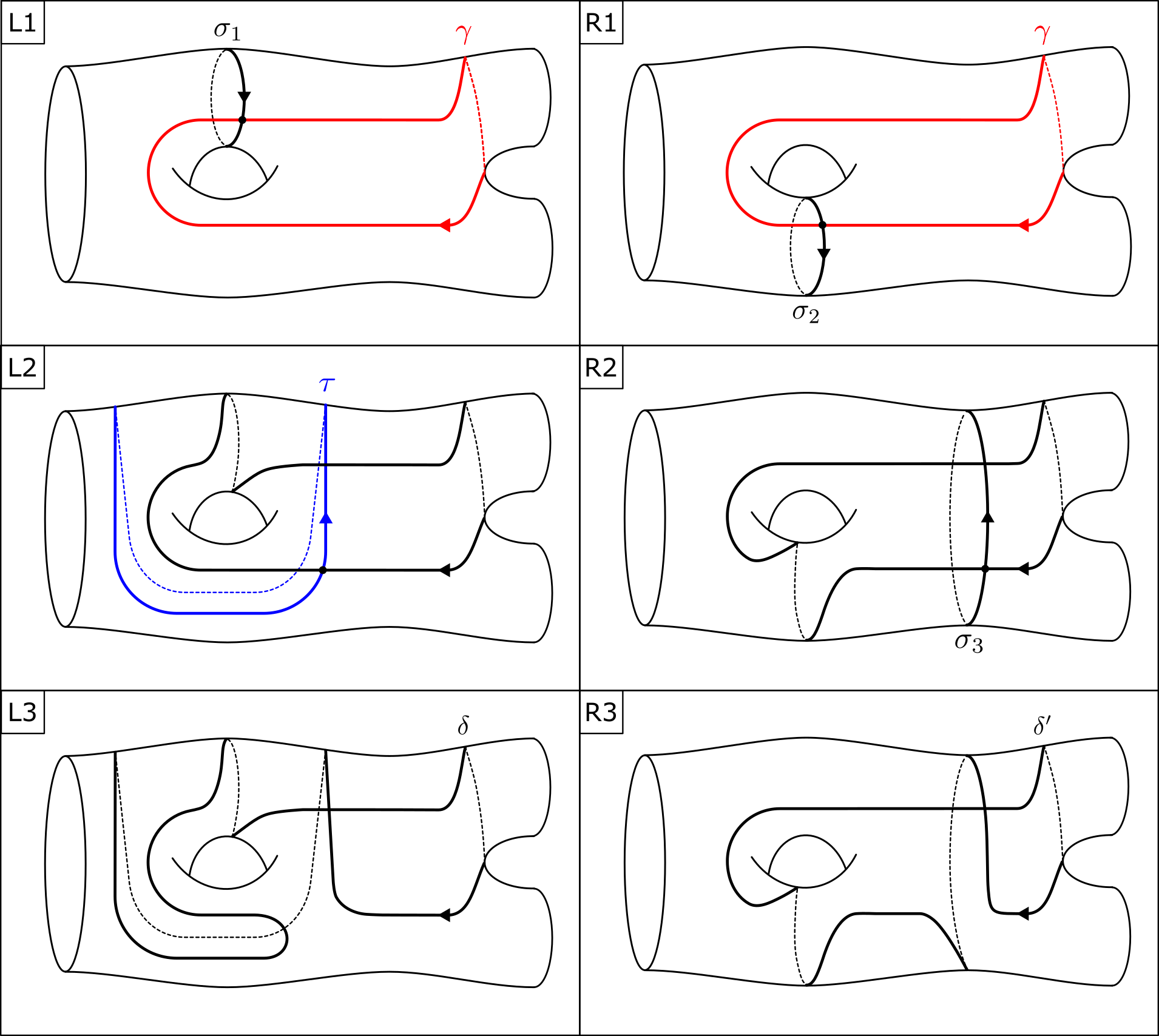
Figure 12. The surgeries used in the proof of Lemma 9.3 in the case $g\geq 3$. This figure is adapted from Figure 15 of [Abo08].

Figure 13. The curves used in the proof of Lemma 9.3 in the case $g=2$. This figure is adapted from Figure 16 of [Abo08].

∎

Lemma 9.4.

Suppose that $\gamma$ is the oriented boundary of an embedded surface $S\subset\Sigma$. Then $[\gamma]=-\chi(S)\,T$ in $\widetilde{\Omega}_{\operatorname{unob}}(\Sigma)$.

Proof.

The proof is by induction on the genus of $S$. If $S$ has genus $1$, this follows from the definition of $T$. Suppose now that $S$ has genus $g(S)>1$. We can write $S=S^{\prime}\cup Q$, where

1. $S^{\prime}$ is a compact surface of genus $g(S^{\prime})=g(S)-1$ and $1$ boundary component $\gamma^{\prime}$.

2. $Q$ is a compact surface of genus $1$ with $2$ boundary components $\gamma$ and $\gamma^{\prime}$.

3. $Q\cap S^{\prime}=\gamma^{\prime}$.

Furthermore, the surface $Q$ can be decomposed as the union of two pairs of pants whose common boundary components are two non-separating curves $\alpha$ and $\beta$. Applying Lemma 9.3 to these pairs of pants and using the induction hypothesis, it follows that

$$[\gamma]=T-[\alpha]-[\beta]=2T+[\gamma^{\prime}]=2T-\chi(S^{\prime})T=-\chi(S)T.$$

∎

Corollary 9.5.

$T$ has order $\chi(\Sigma)$ in $\widetilde{\Omega}_{\operatorname{unob}}(\Sigma)$.

Proof.

Suppose that $\gamma$ bounds a torus in $\Sigma$. Then $\gamma^{-1}$ bounds a surface $S$ with $\chi(S)=\chi(\Sigma)-1$. By Lemma 9.4, we then have

$$-T=[\gamma^{-1}]=-(\chi(\Sigma)-1)\,T,$$

from which it follows that $\chi(\Sigma)T=0$. Moreover, $\mu(T)=-1\in\mathbb{Z}/\chi(\Sigma)\mathbb{Z}$ by Lemma 6.7. Hence $T$ has order $\chi(\Sigma)$. ∎

We can now complete the proof of Proposition 9.2.

Proof of Proposition 9.2..

If $\gamma$ is a separating curve, then by Lemma 9.4 $[\gamma]$ lies in the subgroup generated by $T$.

Suppose now that $\gamma$ is a non-separating curve. Since $\operatorname{Diff}^{+}(\Sigma)$ acts transitively on non-separating curves, $\gamma$ can be obtained from $\alpha_{1}$ by an isotopy and a sequence of Dehn twists about the Lickorish generators. By the Dehn twist formula (11), $[\gamma]$ belongs to the subgroup generated by the classes of the Lickorish generators. By Lemma 9.3, the Lickorish generators satisfy the relation $-[\alpha_{i}]+[\gamma_{i}]+[\alpha_{i+1}]=T$. Hence, we conclude that $[\gamma]$ belongs to the subgroup generated by $T$ and $[\alpha_{i}]$, $[\beta_{i}]$, $i=1,\ldots,g$. ∎

9.2. End of the proof of Theorem B and Corollary C

Proof of Theorem B.

By the results of Section 7, there is a diagram with split-exact rows

Hence, it suffices to prove that the map $\varphi:\widetilde{\Omega}_{\operatorname{unob}}(\Sigma)\to H_{1}(S\Sigma;\mathbb{Z})$ is an isomorphism. This map is surjective by Corollary 6.8. To prove that it is injective, suppose that $A$ belongs to the kernel of $\varphi$. By Proposition 9.2, we can write $A$ in terms of the generators

$$A=k\,T+\sum_{i=1}^{g}n_{i}\,[\alpha_{i}]+m_{i}[\beta_{i}].$$

By projecting to $H_{1}(\Sigma;\mathbb{Z})$, we have the relation

$$\sum_{i=1}^{g}n_{i}\,[\alpha_{i}]+m_{i}[\beta_{i}]=0\in H_{1}(\Sigma;\mathbb{Z}).$$

Since the classes $[\alpha_{i}]$ and $[\beta_{i}]$ form a basis of $H_{1}(\Sigma;\mathbb{Z})$, we deduce that $n_{i}=m_{i}=0$ for all $i=1,\ldots,g$. Hence $A=k\,T$. By Lemma 6.7, we then have $0=\mu(A)=-k\mod\chi(\Sigma)$. Since $T$ has order $\chi(\Sigma)$ by Corollary 9.5, we conclude that $A=0$. ∎

Proof of Corollary C.

By Proposition 6.1 of [Abo08], the invariants introduced in Section 6 descend to surjective morphisms $K_{0}\operatorname{DFuk}(\Sigma)\to\mathbb{R}$ and $K_{0}\operatorname{DFuk}(\Sigma)\to H_{1}(S\Sigma;\mathbb{Z})$. Hence, there is a diagram

It follows that $\Theta$ is an isomorphism. ∎

Appendix A Action-type invariants of Lagrangians in monotone manifolds

In this appendix, we define real-valued Lagrangian cobordism invariants of oriented Lagrangian immersions $L\looparrowright M$, where $M$ is a monotone symplectic manifold. These invariants arise as characteristic numbers associated to a cohomology class which generalizes the action class $[\lambda|_{L}]\in H^{1}(L;\mathbb{R})$ associated to a Lagrangian immersion into an exact symplectic manifold $(M,d\lambda)$. The invariants defined here also generalize the holonomy of an immersed curve in a closed surface of genus $g\neq 1$, as defined in Section 6.2.

Remark A.1.

The reader should be aware that we will only make use of the special case of surfaces of genus $g\geq 2$ in this paper. However, the case of general monotone manifolds is of independent interest and, to the best of the author’s knowledge, does not appear in the litterature.

For the rest of this appendix, we assume that $(M,\omega)$ is a monotone symplectic manifold, in the sense that there is a constant $\tau\in\mathbb{R}$ such that $[\omega]=\tau\,c_{1}(M)$ as elements of $H^{2}(M;\mathbb{R})$.

A.1. Definition of the action class

Let $\mathcal{L}M$ be the (unoriented) Lagrangian Grassmannian of $M$ and $\pi:\mathcal{L}M\to M$ be the projection. The key ingredient for the definition of the action is the following elementary fact.

Lemma A.2.

For any symplectic manifold $M$, $2\,\pi^{*}c_{1}(M)=0$ in $H^{2}(\mathcal{L}M;\mathbb{Z})$.

Proof.

Equip $TM$ with a compatible almost complex structure. Then the Hermitian bundle $\pi^{*}TM$ has a Lagrangian subbundle given by the tautological bundle $\gamma$ over $\mathcal{L}M$. Hence, there is an isomorphism of complex bundles $\pi^{*}TM\cong\gamma\otimes\mathbb{C}$. The lemma then follows from the well-known fact that the odd Chern classes of complexifications have order that divides $2$. ∎

Corollary A.3.

Let $(M,\omega)$ be a monotone symplectic manifold. Then $\pi^{*}\omega$ is exact.

Although Corollary A.3 will be sufficient for our purposes, it is interesting to note that the exactness of $\pi^{*}\omega$ actually characterizes monotonicity.

Proposition A.4.

$(M,\omega)$ is monotone if and only if $\pi^{*}\omega$ is exact.

Proof.

It suffices to show that the kernel of $\pi^{*}:H^{2}(M;\mathbb{R})\to H^{2}(\mathcal{L}M;\mathbb{R})$ is the subspace generated by $c_{1}(M)$. This follows from the fact that, on the $E_{2}$ page of the Serre spectral sequence of the fibration $\pi$, the Maslov class $\mu\in H^{1}(\Lambda_{n};\mathbb{Z})$ transgresses to $\pm 2c_{1}(M)$ (this appears to be well-known; see e.g. Proposition 1 of the appendix of [Vit87]). ∎

A primitive of $\pi^{*}\omega$ will be called an action form. Using such a primitive, we can define the action of Lagrangian immersions in $M$.

Definition A.5.

Let $f:L\to M$ be a Lagrangian immersion. The action of $f$ with respect to the action form $\lambda$ is the class

$$a_{\lambda}(f)=[\widetilde{f}^{*}\lambda]\in H^{1}(L;\mathbb{R}),$$

where $\widetilde{f}:L\to\mathcal{L}M$ is the Gauss map of $f$.

Remark A.6.

The action depends on the choice of the primitive $\lambda$. If $\lambda$ and $\lambda^{\prime}$ are two primitives, then $\lambda-\lambda^{\prime}$ is closed and defines a class $\delta=[\lambda-\lambda^{\prime}]\in H^{1}(\mathcal{L}M;\mathbb{R})$. Then, for a Lagrangian immersion $f$ we have

$$a_{\lambda}(f)-a_{\lambda^{\prime}}(f)=\widetilde{f}^{*}\delta.$$

In particular, if $\delta=0$, i.e. $\lambda$ and $\lambda^{\prime}$ differ by an exact form, then $\lambda$ and $\lambda^{\prime}$ define the same action class.

Remark A.7.

In the case where the manifold $L$ is oriented, the action of a Lagrangian immersion $f:L\to M$ could alternatively be defined as the class $[\widetilde{f}^{*}\lambda]$, where ${p:\mathcal{L}^{\operatorname{or}}(M)\to M}$ is the oriented Lagrangian Grassmannian bundle, $\lambda$ is a primitive of $p^{*}\omega$ and $\widetilde{f}:L\to\mathcal{L}^{\operatorname{or}}(M)$ is the oriented Gauss map. The two definitions are naturally related by the two-fold covering $\mathcal{L}^{\operatorname{or}}(M)\to\mathcal{L}(M)$. This covering induces an isomorphism on $H^{1}(-;\mathbb{R})$, hence it induces a bijection between the cohomology classes of primitives of $\pi^{*}\omega$ and those of $p^{*}\omega$. As a consequence, for oriented Lagrangians the two definitions are essentially interchangeable.

A.2. Invariance under Lagrangian cobordisms

Our next aim is to prove that action is invariant under Lagrangian cobordisms, in the sense that any Lagrangian cobordism carries a cohomology class that extends the action classes of its ends. To show this, we extend the definition of the action class to Lagrangian cobordisms.

Observe that for a monotone manifold $(M,\omega)$, the product $(\mathbb{C}\times M,\omega_{\mathbb{C}}\oplus\omega)$ is also monotone. Hence, by applying Corollary A.3, we deduce that $\widetilde{\pi}^{*}(\omega_{\mathbb{C}}\oplus\omega)$ is exact, where $\widetilde{\pi}:\mathcal{L}(\mathbb{C}\times M)\to\mathbb{C}\times M$ is the projection of the Lagrangian Grassmannian.

Lemma A.8.

Given an action form $\lambda$, there exists a primitive $\widetilde{\lambda}$ of $\widetilde{\pi}^{*}(\omega_{\mathbb{C}}\oplus\omega)$ such that $i^{*}\widetilde{\lambda}-\lambda$ is exact, where $i:\mathcal{L}(M)\to\mathcal{L}(\mathbb{C}\times M)$ is the stabilization map.

Proof.

The map $i$ induces an isomorphism on $\pi_{1}$ (see the proof of Lemma 6.1, which also applies to the unoriented case). Hence, $i$ also induces an isomorphism on $H^{1}(-;\mathbb{R})$. Therefore, $i$ induces a bijection between the cohomology classes of primitives of $\widetilde{\pi}^{*}(\omega_{\mathbb{C}}\oplus\omega)$ and those of $\pi^{*}\omega=\iota^{*}\widetilde{\pi}^{*}(\omega_{\mathbb{C}}\oplus\omega)$. ∎

We fix a primitive $\widetilde{\lambda}$ which is compatible with $\lambda$ as in Lemma A.8. We can now define the action class of a Lagrangian cobordism $F:V\to\mathbb{C}\times M$ by setting

$$a_{\tilde{\lambda}}(F)=[\widetilde{F}^{*}\widetilde{\lambda}]\in H^{1}(V;\mathbb{R}),$$

where $\widetilde{F}:V\to\mathcal{L}(\mathbb{C}\times M)$ is the Gauss map of $F$.

Lemma A.9.

Let $f_{k}:L_{k}\to M$, $k=1,\ldots,r$, be Lagrangian immersions and $F:(f_{1},\ldots,f_{r})\rightsquigarrow\emptyset$ be a Lagrangian cobordism. Then

$$a_{\tilde{\lambda}}(F)|_{L_{k}}=a_{\lambda}(f_{k}).$$

Proof.

By definition, the Gauss map of the cobordism satisfies $\widetilde{F}|_{L_{k}}=i\circ\widetilde{f}_{k}$. Therefore, since $i^{*}\widetilde{\lambda}-\lambda$ is exact, we have

$$a_{\tilde{\lambda}}(F)|_{L_{k}}=[f_{k}^{*}i^{*}\widetilde{\lambda}]=[f_{k}^{*}\lambda]=a_{\lambda}(f_{k}).$$

∎

In the usual fashion, Lemma A.9 allows us to define cobordism invariants of oriented Lagrangian immersions as characteristic numbers involving the action class.

Corollary A.10.

Let $x\in H^{n-1}(\mathcal{L}M;\mathbb{R})$ be a stable class, i.e. $x$ is in the image of the stabilization map $\mathcal{L}M\to\mathcal{L}(\mathbb{C}\times M)$. Let $f:L\to M$ be an oriented Lagrangian immersion. Then the number

$$\langle a_{\lambda}(f)\cup\widetilde{f}^{*}x,[L]\rangle\in\mathbb{R}$$

is an invariant of oriented Lagrangian cobordism.

As a special case, when $M$ is a closed surface of genus $g\neq 1$ and we take $x=1$, we recover the holonomy of immersed curves in $M$, as defined in Section 6.2.

A.3. Action is a primitive of flux

As in the exact case, the action class determines the flux of Lagrangian paths in $M$. Recall that the flux of a path of Lagrangian immersions $f:L\times I\to M$ is the class $\operatorname{flux}(f)\in H^{1}(L;\mathbb{R})$ whose value on a loop $\gamma$ in $L$ is given by

$$\operatorname{flux}(f)\cdot\gamma=\int_{\gamma\times I}f^{*}\omega.$$

See for example [Sol13] for a more detailed discussion of Lagrangian flux.

The flux of a path is invariant under homotopies with fixed endpoints. Hence, for a given manifold $L$, one can see flux as an $H^{1}(L;\mathbb{R})$-valued cocycle on the space of Lagrangian immersions $L\to M$. The next proposition asserts that the action is a primitive of this cocycle.

Proposition A.11.

Let $f:L\times I\to M$ be a Lagrangian path. Then

$$\operatorname{flux}(f)=a_{\lambda}(f_{1})-a_{\lambda}(f_{0}).$$

Proof.

By taking Gauss maps, $f$ lifts to a path $\widetilde{f}:L\times I\to\mathcal{L}M$. Then, for any loop $\gamma$ in $L$ we have

$$\operatorname{flux}(f)\cdot\gamma=\int_{\gamma\times I}f^{*}\omega=\int_{\gamma\times I}\widetilde{f}^{*}\pi^{*}\omega\stackrel{{\scriptstyle\text{Stokes}}}{{=}}\int_{\gamma}\widetilde{f}_{1}^{*}\lambda-\int_{\gamma}\widetilde{f}_{0}^{*}\lambda=a_{\lambda}(f_{1})\cdot\gamma-a_{\lambda}(f_{0})\cdot\gamma.$$

∎

Corollary A.12.

Let $(M,\omega)$ be a monotone manifold and $f:L\times I\to M$ be a Lagrangian loop. Then $\operatorname{flux}(f)=0$.

Appendix B Proof of Proposition 7.6

In this appendix, we prove Proposition 7.6. The proofs given here elaborate and simplify the arguments used by Perrier in the proofs of Proposition 5.4 and Lemma 5.15 of [Per19]. Our main purpose is to give complete proofs that the cobordisms constructed in [Per19] are unobstructed in the sense of Definition 3.3.

We start by proving the proposition in the case of non-separating curves in Section B.1. The case of separating curves will be deduced from the non-separating case in Section B.2.

B.1. Non-separating case

Let $(\alpha,\widetilde{\alpha})$ and $(\beta,\widetilde{\beta})$ be two pairs of isotopic non-separating curves with $\operatorname{Hol}(\widetilde{\alpha})-\operatorname{Hol}(\alpha)=\operatorname{Hol}(\widetilde{\beta})-\operatorname{Hol}(\beta)=x$. We wish to show that

$$[\widetilde{\alpha}]-[\alpha]=[\widetilde{\beta}]-[\beta]$$

in $\Omega_{\operatorname{unob}}(\Sigma)$.

The first case to consider is when $x=0$. By Lemma 7.3, we then have that $\alpha$ is Hamiltonian isotopic to $\widetilde{\alpha}$ and $\beta$ is Hamiltonian isotopic to $\widetilde{\beta}$. It follows that $[\widetilde{\alpha}]-[\alpha]=0=[\widetilde{\beta}]-[\beta]$ and Proposition 7.6 is proved in this case. Hence, from now on we will assume that $x\neq 0$.

The general case of Proposition 7.6 will be deduced from two special cases, which are stated as Lemma B.1 and Lemma B.2 below.

Lemma B.1.

Let $(\alpha,\widetilde{\alpha})$ and $(\beta,\widetilde{\beta})$ be two pairs of isotopic non-separating curves such that $\operatorname{Hol}(\widetilde{\alpha})-\operatorname{Hol}(\alpha)=\operatorname{Hol}(\widetilde{\beta})-\operatorname{Hol}(\beta)$. Furthermore, suppose that

1. $\beta$ and $\widetilde{\beta}$ are disjoint,

2. $\alpha$ is disjoint from $\beta\cup\widetilde{\beta}$.

Then $[\widetilde{\alpha}]-[\alpha]=[\widetilde{\beta}]-[\beta]$ in $\Omega_{\operatorname{unob}}(\Sigma)$.

Proof.

We use the same surgery procedure as in the proof of Proposition 5.4 in [Per19]. The hypothesis implies that there is a curve $\gamma$ that intersects each of the three curves $\alpha$, $\beta$ and $\widetilde{\beta}$ in one point. We may assume that $\gamma$ intersects each curve positively. We then perform the following surgeries, which are illustrated in Figure 14.

Figure 14. The surgery procedure used in the proof of Lemma B.1.

1. The successive surgeries of $\gamma$ with $\alpha$, $\beta^{-1}$ and $\widetilde{\beta}$ at their unique intersection point, producing a curve $\delta$.

2. The surgery of $\delta$ with a curve $\widetilde{\gamma}$ which is Hamiltonian isotopic to $\gamma^{-1}$ and intersects $\delta$ in one point lying on $\alpha$. This produces a curve $\tau$.

Since all the curves involved in the above surgeries intersect only once, the associated surgery cobordisms are embedded. Moreover, the cobordisms are incompressible by Lemma 5.9. Hence, by concatenating these cobordisms and using Proposition 4.11, we obtain an unobstructed cobordism $\tau\rightsquigarrow(\beta^{-1},\gamma,\alpha,\widetilde{\beta},\widetilde{\gamma})$. This gives the relation $[\tau]=[\alpha]+[\widetilde{\beta}]-[\beta]$.

It is easy to check that the curve $\tau$ is isotopic to $\alpha$, hence also isotopic to $\widetilde{\alpha}$. Moreover, by the holonomy assumption we have

$$\operatorname{Hol}(\tau)=\operatorname{Hol}(\alpha)+\operatorname{Hol}(\widetilde{\beta})-\operatorname{Hol}(\beta)=\operatorname{Hol}(\widetilde{\alpha}).$$

Hence, by Lemma 7.3, $\tau$ is Hamiltonian isotopic to $\widetilde{\alpha}$ and the conclusion follows. ∎

Lemma B.2.

Let $(\alpha,\widetilde{\alpha})$ and $(\beta,\widetilde{\beta})$ be two pairs of isotopic non-separating curves such that $\operatorname{Hol}(\widetilde{\alpha})-\operatorname{Hol}(\alpha)=\operatorname{Hol}(\widetilde{\beta})-\operatorname{Hol}(\beta)$. Suppose that $\alpha\cap\widetilde{\alpha}=\emptyset=\beta\cap\widetilde{\beta}$.

Then $[\widetilde{\alpha}]-[\alpha]=[\widetilde{\beta}]-[\beta]$ in $\Omega_{\operatorname{unob}}(\Sigma)$.

Proof.

By Theorem 4.4 of [FM12], there is a sequence of non-separating curves $(\gamma_{j})_{j=0}^{\ell}$ such that $\gamma_{0}=\alpha$, $\gamma_{\ell}=\beta$ and $\gamma_{j}\cap\gamma_{j+1}=\emptyset$ for $j=0,\ldots,\ell-1$.

For any integer $N$, we can write

$$[\widetilde{\alpha}]-[\alpha] =N\;\left(\,[\alpha^{\prime}]-[\alpha]\,\right)$$

where $\alpha^{\prime}$ is isotopic to $\alpha$ and $\alpha\cap\alpha^{\prime}=\emptyset$. Indeed, since $\alpha\cap\widetilde{\alpha}=\emptyset$, there is an isotopy $(\alpha_{t})_{t\in[0,1]}$ such that $\alpha_{0}=\alpha$, $\alpha_{1}=\widetilde{\alpha}$ and the corresponding map $S^{1}\times[0,1]\to\Sigma$ is an embedding (see Lemma 2.4 of [Eps66]). Pick a subdivision $t_{0}=0<t_{1}<\ldots<t_{N}=1$ of the interval $[0,1]$ with the property that

$$\operatorname{Hol}(\alpha_{t_{i+1}})-\operatorname{Hol}(\alpha_{t_{i}})=\frac{x}{N}$$

for $i=0,\ldots,N-1$. Applying Lemma B.1 to the pairs $(\alpha,\alpha_{t_{1}})$ and $(\alpha_{t_{i}},\alpha_{t_{i+1}})$, we have

$$[\widetilde{\alpha}]-[\alpha] =\sum_{i=0}^{N-1}[\alpha_{t_{i+1}}]-[\alpha_{t_{i}}]$$

$$=N\;\left(\,[\alpha_{t_{1}}]-[\alpha]\,\right)$$

Likewise, we can write $[\widetilde{\beta}]-[\beta]=N\,\left([\beta^{\prime}]-[\beta]\right)$.

By choosing $N$ large enough, we can assume that each curve $\gamma_{j}$ has a tubular neighbordhood $A_{j}$ such that the two components of $A_{j}\setminus\gamma_{j}$ have area greater than $|x|/N$, and moreover that $A_{j}\cap A_{j+1}=\emptyset$. In particular, for each $j=0,\ldots,\ell$ there is a curve $\widetilde{\gamma}_{j}$ with the following properties:

1. $\operatorname{Hol}(\widetilde{\gamma}_{j})-\operatorname{Hol}(\gamma_{j})=\frac{x}{N}$,

2. $\widetilde{\gamma}_{j}\cap\gamma_{j}=\emptyset$,

3. $(\gamma_{j},\widetilde{\gamma}_{j})$ is disjoint from $(\gamma_{j+1},\widetilde{\gamma}_{j+1})$.

The result now follows from applying Lemma B.1 successively to the pairs $(\alpha,\alpha^{\prime})$, $(\gamma_{1},\widetilde{\gamma}_{1})$, $(\gamma_{2},\widetilde{\gamma}_{2})$, $\ldots$ , $(\beta,\beta^{\prime})$.

∎

Lemma B.3.

There is a constant $c>0$ with the following property: for each non-separating curve $\alpha$ and each $x\in\mathbb{R}$ with $|x|<c$, there is a curve $\widetilde{\alpha}$ isotopic to $\alpha$ such that $\alpha\cap\widetilde{\alpha}=\emptyset$ and $\operatorname{Hol}(\widetilde{\alpha})-\operatorname{Hol}(\alpha)=x$.

Proof.

For a given curve $\alpha$, there is a Weinstein neighborhood $U$ and a symplectomorphism $\varphi:U\cong(-c,c)\times S^{1}$ such that $\varphi(\alpha)=\{0\}\times S^{1}$. Then the required curves $\widetilde{\alpha}$ are obtained by pushing $\alpha$ in the radial direction of the annulus. The same constant $c$ works for all non-separating curves, since all non-separating curves on a closed surface are symplectomorphic. ∎

Remark B.4.

The optimal constant in the preceding lemma is $c=\operatorname{area}(\Sigma)$, but we will not make use of this.

We now proceed to the proof of Proposition 7.6 in the case of non-separating curves.

Proof of Proposition 7.6 – non-separating case..

Pick a constant $c$ as in Lemma B.3. By choosing isotopies from $\alpha$ to $\widetilde{\alpha}$ and from $\beta$ to $\widetilde{\beta}$ and breaking them into isotopies of small flux, it suffices to prove the proposition when the holonomy difference satisfies $|x|<c$.

By our choice of $c$, there is a curve $\widehat{\alpha}$ isotopic to $\alpha$ such that $\widehat{\alpha}\cap\alpha=\emptyset$ and

$$\operatorname{Hol}(\widehat{\alpha})-\operatorname{Hol}(\alpha)=x.$$

In particular, $\widehat{\alpha}$ is Hamiltonian isotopic to $\widetilde{\alpha}$, so $[\widehat{\alpha}]=[\widetilde{\alpha}]$. Likewise, there is a curve $\widehat{\beta}$ isotopic to $\beta$ such that $\widehat{\beta}\cap\beta=\emptyset$ and $[\widehat{\beta}]=[\widetilde{\beta}]$. The proposition now follows by applying Lemma B.2 to the pairs $(\alpha,\widehat{\alpha})$ and $(\beta,\widehat{\beta})$. ∎

B.2. Separating case

The following lemma reduces Proposition 7.6 in the case of separating curves to the non-separating case.

Lemma B.5.

Let $\alpha$ and $\widetilde{\alpha}$ be isotopic non-contractible separating curves. Then there are isotopic non-separating curves $\gamma$ and $\widetilde{\gamma}$ such that

$$[\widetilde{\alpha}]-[\alpha]=[\widetilde{\gamma}]-[\gamma].$$

Proof.

The proof uses a simpler version of the surgery procedure described in the proof of Lemma 5.15 of [Per19]. We start by showing that for a given separating curve $\alpha$, there is a number $\varepsilon(\alpha)>0$ such that the lemma holds for any curve $\widetilde{\alpha}$ isotopic to $\alpha$ that satisfies $|\operatorname{Hol}(\widetilde{\alpha})-\operatorname{Hol}(\alpha)|<\varepsilon(\alpha)$.

Since $\alpha$ is separating and non-contractible, there is a non-separating curve $\gamma$ such that $\alpha$ and $\gamma$ intersect twice and are in minimal position. We are therefore in the setting considered in Section 8.2. We perform the following surgeries, which are a small modification of the procedure described in Section 8.2. The whole procedure is illustrated in Figure 15.

Figure 15. The surgery procedure used in the proof of Lemma B.5.

Let $s_{1}$ be the negative intersection point of $(\alpha,\gamma)$, and $q_{1}$ be the positive intersection. The first step is to form the surgery $\sigma=\alpha\#_{s_{1}}\gamma^{-1}$. Next, by considering small pushoffs of $\gamma$, we can find an $\varepsilon>0$ with the property that for any $x$ with $|x|<\varepsilon$, there is a curve $\widetilde{\gamma}$ isotopic to $\gamma$ that satisfies

1. $\operatorname{Hol}(\widetilde{\gamma})-\operatorname{Hol}(\gamma)=x$,

2. $\widetilde{\gamma}$ intersects $\sigma$ in two points; the first one, denoted $s_{2}$, lies on the arc of $\gamma$ near $q_{1}$, and the other, denoted $q_{2}$, lies on the arc of $\alpha$ near $q_{1}$.

Given such a curve $\widetilde{\gamma}$, we let $\tau=\widetilde{\gamma}\#_{s_{2}}\sigma$. The size of the surgery handle is chosen big enough so that $\tau$ is embedded.

The curve $\tau$ is isotopic to $\alpha$. Moreover, there is an immersed cobordism $\tau\rightsquigarrow(\widetilde{\gamma},\alpha,\gamma^{-1})$. The unobstructedness arguments used in Section 8.2 apply verbatim to the present case, and we conclude that there is an unobstructed cobordism with the same ends. Hence, we obtain the relation $[\tau]-[\alpha]=[\widetilde{\gamma}]-[\gamma]$. Moreover, we have

$$\operatorname{Hol}(\tau)=\operatorname{Hol}(\alpha)+\operatorname{Hol}(\widetilde{\gamma})-\operatorname{Hol}(\gamma)=\operatorname{Hol}(\alpha)+x.$$

Suppose now that $\widetilde{\alpha}$ is any curve isotopic to $\alpha$ with $\operatorname{Hol}(\widetilde{\alpha})-\operatorname{Hol}(\alpha)=x$ and $|x|<\varepsilon$. Then we have

$$\operatorname{Hol}(\widetilde{\alpha})=\operatorname{Hol}(\alpha)+x=\operatorname{Hol}(\tau),$$

so $\tau$ is Hamiltonian isotopic to $\widetilde{\alpha}$ by Lemma 7.3. Hence, we obtain the required relation $[\widetilde{\alpha}]-[\alpha]=[\gamma]-[\widetilde{\gamma}]$.

If $\beta$ is a curve sufficiently $C^{1}$-close to $\alpha$, then the preceding construction still works with the same choices of $\gamma$ and $\widetilde{\gamma}$. In particular, this means that the function $\varepsilon(\alpha)$ can be chosen to be lower-semicontinuous in the $C^{1}$ topology.

Consider now the general case where $\alpha$ and $\widetilde{\alpha}$ are arbitrary isotopic separating curves. Choose an isotopy $(\alpha_{t})_{t\in[0,1]}$ from $\alpha$ to $\widetilde{\alpha}$. Then $\varepsilon(\alpha_{t})$ is bounded away from $0$, hence there is a subdivision $t_{0}=0<t_{1}<\ldots<t_{N}=1$ of the interval such that

$$|\operatorname{Hol}(\alpha_{t_{i+1}})-\operatorname{Hol}(\alpha_{t_{i}})|<\varepsilon(\alpha_{t_{i}})$$

for $i=0,\ldots,N-1$. The lemma now follows by applying the preceding case to each pair $(\alpha_{t_{i}},\alpha_{t_{i+1}})$. ∎

References

- [Abo08] M. Abouzaid. On the Fukaya categories of higher genus surfaces. Adv. Math., 217(3):1192–1235, 2008.
- [AJ10] M. Akaho and D. Joyce. Immersed Lagrangian Floer theory. J. Differential Geom., 86(3):381–500, 2010.
- [Aka05] M. Akaho. Intersection theory for Lagrangian immersions. Math. Res. Lett., 12(4):543–550, 2005.
- [Arn80] V. I. Arnol’d. Lagrange and Legendre cobordisms. I. Funktsional. Anal. i Prilozhen., 14(3):1–13, 96, 1980.
- [AS01] M. Akveld and D. Salamon. Loops of Lagrangian submanifolds and pseudoholomorphic discs. Geom. Funct. Anal., 11(4):609–650, 2001.
- [Aud87] M. Audin. Cobordismes d’immersions lagrangiennes et legendriennes, volume 20 of Travaux en Cours. Hermann, Paris, 1987.
- [Aud90] M. Audin. Quelques remarques sur les surfaces lagrangiennes de Givental’. J. Geom. Phys., 7(4):583–598 (1991), 1990.
- [BC13] P. Biran and O. Cornea. Lagrangian cobordism. I. J. Amer. Math. Soc., 26(2):295–340, 2013.
- [BC14] P. Biran and O. Cornea. Lagrangian cobordism and Fukaya categories. Geom. Funct. Anal., 24(6):1731–1830, 2014.
- [BC17] P. Biran and O. Cornea. Cone-decompositions of Lagrangian cobordisms in Lefschetz fibrations. Selecta Math. (N.S.), 23(4):2635–2704, 2017.
- [BC21] P. Biran and O. Cornea. A Lagrangian pictionary. Kyoto J. Math., 61(2):399–493, 2021.
- [BCS21] P. Biran, O. Cornea, and E. Shelukhin. Lagrangian shadows and triangulated categories. Astérisque, (426):128, 2021.
- [Bos21] V. Bosshard. Lagrangian cobordisms in Liouville manifolds. Preprint, can be found at arXiv:2105.14821, 2021.
- [Chi72] D. R. J. Chillingworth. Winding numbers on surfaces. I. Math. Ann., 196:218–249, 1972.
- [Eli84] Y. Eliashberg. Cobordisme des solutions de relations différentielles. In South Rhone seminar on geometry, I (Lyon, 1983), Travaux en Cours, pages 17–31. Hermann, Paris, 1984.
- [Eps66] D. B. A. Epstein. Curves on -manifolds and isotopies. Acta Math., 115:83–107, 1966.
- [FM12] B. Farb and D. Margalit. A primer on mapping class groups, volume 49 of Princeton Mathematical Series. Princeton University Press, Princeton, NJ, 2012.
- [FOOO09] K. Fukaya, Y.-G. Oh, H. Ohta, and K. Ono. Lagrangian intersection Floer theory: anomaly and obstruction, volume 46 of AMS/IP Studies in Advanced Mathematics. American Mathematical Society, Providence, RI; International Press, Somerville, MA, 2009.
- [GT23] Y. Ganor and S. Tanny. Floer theory of disjointly supported Hamiltonians on symplectically aspherical manifolds. Algebr. Geom. Topol., 23(2):645–732, 2023.
- [Hau15] L. Haug. The Lagrangian cobordism group of . Selecta Math. (N.S.), 21(3):1021–1069, 2015.
- [Hen20] F. Hensel. Stability conditions and Lagrangian cobordisms. J. Symplectic Geom., 18(2):463–536, 2020.
- [Hic22a] J. Hicks. Lagrangian cobordisms and lagrangian surgery. Preprint, can be found at arXiv:2102.10197, 2022.
- [Hic22b] J. Hicks. Wall-crossing from lagrangian cobordisms. Preprint, can be found at arXiv:1911.09979, 2022.
- [IS02] S. Ivashkovich and V. Shevchishin. Reflection principle and -complex curves with boundary on totally real immersions. Commun. Contemp. Math., 4(1):65–106, 2002.
- [Jac70] W. Jaco. On certain subgroups of the fundamental group of a closed surface. Proc. Cambridge Philos. Soc., 67:17–18, 1970.
- [Lic64] W. B. R. Lickorish. A finite set of generators for the homeotopy group of a -manifold. Proc. Cambridge Philos. Soc., 60:769–778, 1964.
- [LS91] F. Lalonde and J.-C. Sikorav. Sous-variétés lagrangiennes et lagrangiennes exactes des fibrés cotangents. Comment. Math. Helv., 66(1):18–33, 1991.
- [Mil65] J. Milnor. Lectures on the -cobordism theorem. Princeton University Press, Princeton, N.J.,, 1965. Notes by L. Siebenmann and J. Sondow.
- [MS17] D. McDuff and D. A. Salamon. Introduction to symplectic topology. Oxford Graduate Texts in Mathematics. Oxford University Press, Oxford, third edition, 2017.
- [MW18] C. Y. Mak and W. Wu. Dehn twist exact sequences through Lagrangian cobordism. Compos. Math., 154(12):2485–2533, 2018.
- [NT20] D. Nadler and H. L. Tanaka. A stable -category of Lagrangian cobordisms. Adv. Math., 366:107026, 97, 2020.
- [Per19] A. Perrier. Lagrangian cobordism groups of higher genus surfaces. Preprint, can be found at arXiv:1901.06002, 2019.
- [Pol91] L. Polterovich. The surgery of Lagrange submanifolds. Geom. Funct. Anal., 1(2):198–210, 1991.
- [Rei60] B. L. Reinhart. The winding number on two manifolds. Ann. Inst. Fourier (Grenoble), 10:271–283, 1960.
- [Sei00] P. Seidel. Graded Lagrangian submanifolds. Bull. Soc. Math. France, 128(1):103–149, 2000.
- [Sei08] P. Seidel. Fukaya categories and Picard-Lefschetz theory. Zurich Lectures in Advanced Mathematics. European Mathematical Society (EMS), Zürich, 2008.
- [Sei11] P. Seidel. Homological mirror symmetry for the genus two curve. J. Algebraic Geom., 20(4):727–769, 2011.
- [Sol13] J. P. Solomon. The Calabi homomorphism, Lagrangian paths and special Lagrangians. Math. Ann., 357(4):1389–1424, 2013.
- [SS21] N. Sheridan and I. Smith. Lagrangian cobordism and tropical curves. J. Reine Angew. Math., 774:219–265, 2021.
- [Vit87] C. Viterbo. Intersection de sous-variétés lagrangiennes, fonctionnelles d’action et indice des systèmes hamiltoniens. Bull. Soc. Math. France, 115(3):361–390, 1987.