Primordial black holes from a curvaton scenario with strongly non-Gaussian perturbations

Abstract

We investigate the production of primordial black holes (PBHs) in a mixed inflaton–curvaton scenario with a quadratic curvaton potential, assuming the curvaton is in de Sitter equilibrium during inflation with $\langle\chi\rangle=0$. In this setup, the curvature perturbation sourced by the curvaton is strongly non-Gaussian, containing no leading Gaussian term. We show that for $m^{2}/H^{2}\gtrsim 0.3$, the curvaton contribution to the spectrum of primordial perturbations on CMB scales can be kept negligible but on small scales the curvaton can source PBHs. In particular, PBHs in the asteroid mass range $10^{-16}M_{\odot}\lesssim M\lesssim 10^{-10}M_{\odot}$ with an abundance reaching $f_{\rm PBH}=1$ can be produced when the inflationary Hubble scale $H\gtrsim 10^{12}$ GeV and the curvaton decay occurs in the window from slightly before the electroweak transition to around the QCD transition.

1 Introduction

The study of primordial black holes (PBHs) formed via gravitational collapse of large primordial density fluctuations was initiated over $50$ years ago [1, 2]. Already in [3] it was proposed that PBHs could form a cold dark matter component in the universe. The possibility that PBHs of mass $M\gtrsim 10^{-10}M_{\odot}$ would constitute all of the dark matter is already ruled out by constraints from lensing, dynamical effects, structure formation and gravitational waves [4]. In the asteroid mass window, $10^{-16}M_{\odot}\lesssim M\lesssim 10^{-10}M_{\odot}$ the constraints are uncertain and it is possible that PBHs with masses in this range could constitute a dominant dark matter component [4]. Even a subdominant PBH contribution to dark matter can have characteristic observational imprints, such as gravitational waves from PBH mergers testable with LIGO–Virgo–KAGRA data [5, 6, 7, 8, 9]. Observational signals associated to PBHs are among the very few ways to probe small scale primordial perturbations and the process responsible for their generation.

Several mechanisms for producing PBHs have been investigated in the literature, including perturbations produced during inflation [10, 11, 12, 13, 14, 15, 16, 17, 18, 19, 20, 21, 22, 23, 24, 25, 26, 27, 28, 29, 30, 31, 32], cosmic strings  [33, 34, 35], phase transitions [36, 37, 38], dark matter clumps [39], and bouncing cosmologies [40, 41]. In this work, we focus on the curvaton scenario [42, 43, 44, 45, 46]. Several authors have already investigated PBH formation in curvaton models  [47, 48, 49, 50, 51] and other spectator scenarios [52, 53, 54, 55, 56, 57] where the curvature perturbation can acquire non-Gaussian contributions. The effect of this non-Gaussianity is typically treated perturbatively, using the parameters $f_{\text{NL}}$ etc. [58, 59, 60, 61, 62]. Recently, a general non-perturbative formalism for investigating the PBH abundance in the presence of non-Gaussian perturbations has been developed e.g. in [63, 64, 65]. To our knowledge, the previous analyses of PBH production in the curvaton scenario have however focused on the case where the curvaton field has a non-vanishing mean value during inflation, $|\langle\chi\rangle|\gg H$, and the curvature perturbation contains a leading Gaussian part proportional to $\delta\chi/\langle\chi\rangle\ll 1$. The non-Gaussianities can then be accommodated using a truncated expansion around the Gaussian part, although see [48] for a discussion of limitations of this method when $\langle\chi\rangle\gg H$.

In this work, we will study PBH formation in the curvaton setup with a quadratic potential, assuming $\langle\chi\rangle=0$. This is the equilibrium configuration of a light spectator during de Sitter inflation [66], provided the potential is minimized at $\chi=0$. Even if one starts from an initial configuration with a non-zero $\langle\chi\rangle$, the distribution is rapidly driven towards the equilibrium during de Sitter inflation [66, 67]. For $\langle\chi\rangle=0$, perturbations of the curvaton energy density obey the distribution of a squared Gaussian field and are large, $\langle\delta\rho_{\chi}^{2}\rangle/\langle\rho_{\chi}\rangle^{2}=2$ [42]. Consequently, the curvature perturbation component sourced by the curvaton has no leading Gaussian part and it can not be expanded in small perturbations. Therefore, one needs to consider the full non-linear and non-Gaussian solution for the curvature perturbation when investigating the PBH formation. The curvature perturbation $\zeta$ on CMB anisotropy scales is Gaussian to a high precision [69] and contributions sourced by $\delta\rho_{\chi}/\langle\rho_{\chi}\rangle$ must be strongly suppressed on these scales. If the curvaton spectrum is sufficiently blue-tilted, it can however give a dominant contribution to $\zeta$ on small scales $k\gg{\rm Mpc}^{-1}$ where there are no constraints on non-Gaussianity. We focus on such a setup, investigating a mixed inflaton–curvaton scenario with a strongly blue tilted curvaton component which dominates the curvature perturbation on small scales and sources a strongly non-Gaussian $\zeta$ with no leading Gaussian component. On the CMB scales, we require that the spectrum of $\zeta$ is dominated by a Gaussian inflaton component and contributions from the curvaton are suppressed to the $10^{-11}$ level at the CMB pivot scale $k_{*}=0.05\ {\rm Mpc}^{-1}$. We note that PBHs in a partially related phenomenological setup with a Gaussian blue tilted spectator curvature perturbation component was investigated in [54].

We use the $\delta N$ approach [70, 71, 72, 73] to obtain a non-linear solution for the superhorizon scale curvature perturbation. We expand the curvaton field $\chi({\bf x})$ in spherical harmonics and, following [63], truncate the expansion to the monopole when considering fluctuations relevant for PBHs. Within this approximation, we compute the probability distribution for $C_{l}(r)$ which determines the compaction function $C(C_{l}(r))$. The compaction function $C(r)$ equals the comoving gauge density contrast smoothed over a radius $r$. Using $C_{\rm c}=0.55$ [74] as the PBH collapse threshold and modeling the PBH mass with the collapse parameters obtained in [75] for the power law spectrum, we explore the fraction of dark matter in PBHs $f_{\rm PBH}$ and the mass distribution $f(M)$ as functions of the curvaton model parameters. We show that the curvaton scenario with the quadratic potential and the equilibrium configuration $\langle\chi\rangle=0$ can lead to very efficient PBH production. In particular, we find that the scenario can produce asteroid mass PBHs, $10^{-16}M_{\odot}\lesssim M\lesssim 10^{-10}M_{\odot}$, with $f_{\rm PBH}=1$ when the inflationary Hubble scale $H\gtrsim 10^{12}$ GeV, the curvaton mass $m^{2}/H^{2}\gtrsim 0.3$ and the curvaton decay occurs in the window from slightly before the electroweak transition to around the QCD transition.

The paper is organised as follows. In Sec. 2 we present the setup and in Sec. 3 we compute the probability distribution for the compaction function. In Sec. 4 we collect the expressions for the PBH abundance $f_{\rm PBH}$ and the mass distribution $f(M)$. In Sec. 5 we present our main results and summarise the discussion in Sec. 6.

2 The mixed inflaton–curvaton setup

We investigate the PBH abundance in a mixed inflaton–curvaton scenario where the inflaton generates the Gaussian, nearly scale invariant curvature perturbations on CMB scales and curvaton-sourced perturbations dominate on small scales relevant for PBH formation. We assume the quadratic curvaton potential

$$V(\chi)=\frac{1}{2}m^{2}\chi^{2}~{}.$$ (2.1)

We further assume that the curvaton distribution during inflation follows the de Sitter equilibrium result with a vanishing mean value $\langle\chi\rangle=0$ [66]. Ebadi et al. [76] recently examined the production of gravitational waves for this case. For the quadratic potential, the curvaton $\chi$ is a Gaussian field and for $m^{2}/H^{2}<3/2$ its spectrum at the end of inflation on superhorizon scales is given by the standard power-law expression [77]

$${\cal P}_{\chi}(k)=\left(\frac{H}{2\pi}\right)^{2}\left(\frac{k}{k_{\rm end}}\right)^{3-2\nu}\frac{2^{2\nu-1}\Gamma(\nu)^{2}}{\pi}~{},\qquad\nu=\sqrt{\frac{9}{4}-\frac{m^{2}}{H^{2}}}~{}.$$ (2.2)

We denote the Hubble scale at the end of inflation by $H\equiv H(t_{\rm end})$, and $k_{\rm end}=a(t_{\rm end})H(t_{\rm end})$ is the mode exiting the horizon at the end of inflation. Perturbations of the curvaton energy density

$$\frac{\delta\rho_{\chi}({\bf x})}{\langle\rho_{\chi}\rangle}=\frac{\rho_{\chi({\bf x})}-\langle\rho_{\chi}\rangle}{\langle\rho_{\chi}\rangle}=\frac{\chi^{2}({\bf x})}{\langle\chi^{2}\rangle}-1,$$ (2.3)

obey the statistics of a Gaussian squared quantity, and the perturbations are large since $\langle\delta\rho_{\chi}^{2}({\bf x})\rangle/\langle\rho_{\chi}\rangle^{2}=2$. Consequently, any contribution to the curvature perturbation sourced by $\delta\rho_{\chi}/\langle\rho_{\chi}\rangle$ must be suppressed on the large scales $k\lesssim{\rm Mpc^{-1}}$ probed by the CMB and LSS data [69].

Using the $\delta N$ formalism [70, 71, 72, 73], the superhorizon curvature perturbation $\zeta$ in the mixed scenario with inflaton sourced perturbations in the radiation component and the perturbed curvaton component obeys the non-linear equation [78]

$$e^{4\zeta}-\Omega_{\chi}e^{3\zeta_{\chi}}e^{\zeta}+\left(\Omega_{\chi}-1\right)e^{4\zeta_{\rm r}}=0~{}.$$ (2.4)

The individual curvature perturbations of the radiation $\zeta_{\rm r}$ and curvaton $\zeta_{\chi}$ fluids, and $\Omega_{\chi}$ are given in terms of spatially flat gauge quantities by the expressions,

$$\zeta_{\rm r}({\bf x})=\frac{1}{4}{\rm ln}\frac{\rho_{\rm r}({\bf x})}{\langle\rho_{\rm r}\rangle}~{},\qquad\zeta_{\rm\chi}({\bf x})=\frac{1}{3}{\rm ln}\frac{\rho_{\chi}({\bf x})}{\langle\rho_{\chi}\rangle}~{},\qquad\Omega_{\chi}=\frac{\langle\rho_{\chi}\rangle}{\langle\rho_{\rm r}\rangle+\langle\rho_{\chi}\rangle}~{}.$$ (2.5)

Both $\zeta_{\rm r}$ and $\zeta_{\chi}$ are separately conserved, i.e. constant in time. For the quadratic potential Eq. (2.1), the curvaton component $\zeta_{\chi}$ can be written in terms of the field $\chi$ as

$$\zeta_{\chi}=\frac{1}{3}{\rm ln}\frac{\chi^{2}}{\langle\chi^{2}\rangle}~{}.$$ (2.6)

Here and in the rest of the text we use $\chi\equiv\chi_{\rm end}$ to denote the curvaton field at the end of inflation.

The solution for the fourth order algebraic equation (2.4) can be written as [78]

$$\zeta = \zeta_{\rm r}+{\rm ln}\left(K^{1/2}\left(\frac{4-\Omega_{\chi}}{12}\right)^{1/3}\left[1+\left(\frac{3\Omega_{\chi}K^{-3/2}e^{3(\zeta_{\chi}-\zeta_{\rm r})}}{4-\Omega_{\chi}}-1\right)^{1/2}\right]\right)~{},$$ (2.7)

$$K = \frac{1}{2}\left[P^{1/3}+\frac{4\Omega_{\chi}-4}{4-\Omega_{\chi}}\left(\frac{12}{4-\Omega_{\chi}}\right)^{1/3}P^{-1/3}\right]~{},$$

$$P = \left(\frac{3\Omega_{\chi}e^{3(\zeta_{\chi}-\zeta_{\rm r})}}{4-\Omega_{\chi}}\right)^{2}+\left[\left(\frac{3\Omega_{\chi}e^{3(\zeta_{\chi}-\zeta_{\rm r})}}{4-\Omega_{\chi}}\right)^{4}+\frac{12}{4-\Omega_{\chi}}\left(\frac{4-4\Omega_{\chi}}{4-\Omega_{\chi}}\right)^{3}\right]^{1/2}~{}.$$

Here the only time dependent quantity is the curvaton density parameter $\Omega_{\chi}$. Assuming the curvaton is subdominant at the onset of oscillations, which we define as $H(t_{\rm osc})\equiv m$, the density parameter for $t\gg t_{\rm osc}$ can be written as

$$\Omega_{\chi}=\frac{\Omega_{\chi,{\rm osc}}}{\Omega_{\chi,{\rm osc}}+\frac{a_{\rm osc}}{a}}\approx\frac{0.136\langle\chi^{2}\rangle}{0.136\langle\chi^{2}\rangle+\frac{a_{\rm osc}}{a}M_{\rm P}^{2}}~{}.$$ (2.8)

Here we used that $\rho_{\chi,{\rm osc}}\approx(1/2)m^{2}0.816\chi^{2}$ which follows from solving the curvaton equation of motion in a radiation dominated universe. We approximate the curvaton decay as an instant process at $H(t_{\rm dec})=\Gamma$. Within this approximation $\zeta\equiv\zeta(t>t_{\rm dec})=\zeta(t_{\rm dec})$ is obtained by evaluating Eq. (2.7) at the moment $t_{\rm dec}$.

We assume the perturbation of the radiation component $\zeta_{\rm r}$ is entirely sourced by the inflaton and uncorrelated with the curvaton, $\langle\zeta_{\rm r}\zeta_{\chi}\rangle=0$. We further assume $\zeta_{\rm r}$ obeys Gaussian statistics with the power law spectrum

$${\cal P}_{\zeta_{\rm r}}(k)=A_{\rm r}\left(\frac{k}{k_{*}}\right)^{n_{\rm r}-1}~{},$$ (2.9)

where $k_{*}=0.05\ {\rm Mpc}^{-1}$. As explained above, we want to realise a scenario where the Gaussian inflaton sourced perturbations $\zeta_{\rm r}$ dominate the two point function of $\zeta$ on large scales and generate the observed CMB spectrum with $P_{\zeta}(k_{*})=A_{\rm s}=2.10\times 10^{-9},n_{\rm s}=0.965$ [79]. Correspondingly, contributions from $\zeta_{\chi}$ to the spectrum of $\zeta$ must be sufficiently suppressed. To this end, we require

$${\cal P}_{\zeta_{\chi}}(k_{*})<2\times 10^{-11}~{},$$ (2.10)

which, as we show in Appendix B, allows us to obtain the observed CMB spectrum with $A_{\rm r}\sim 10^{-9}$ and $|n_{\rm r}-1|\sim 0.01$, assuming $\Omega_{\chi}$ $\lesssim 0.9$. Note that the underlying computation is somewhat non-trivial as $\zeta$ is a strongly non-linear function of the non-Gaussian $\zeta_{\chi}$. The condition (2.10) constrains the curvaton mass from below as we show in detail in Appendix A, and implies a strongly blue tilted spectrum both for the curvaton field Eq. (2.2) and for $\zeta_{\chi}$. On small scales, $k\gg{\rm Mpc}^{-1}$, the connected correlators of $\zeta$ are dominated by $\zeta_{\chi}$ which, as we show below, can lead to efficient formation of PBHs. For the maximal inflationary Hubble scale $H\approx 5.2\times 10^{13}\;{\rm GeV}$ consistent with the observational bound on the tensor-to-scalar ratio $r_{\rm T}<0.044$ [80], Eq. (2.10) implies $m^{2}/H^{2}\gtrsim 0.29$, assuming instant transition from inflation to radiation domination. The lower bound on $m^{2}/H^{2}$ slowly grows as a function of decreasing $H$. For example, for $H=1.6\times 10^{11}\ {\rm GeV}$, Eq. (2.10) implies $m^{2}/H^{2}\gtrsim 0.31$, see Fig. 6 in Appendix B.

3 Probability distribution of density fluctuations

The central quantity in determining if an overdense region collapses into a primordial black hole is the compaction function $C(r)$ [81, 82, 83] which for spherical overdensities equals the comoving density contrast coarse-grained with a top hat window function over a spherical volume of comoving radius $r$. Denoting the background equation of state by $w=\langle p\rangle/\langle\rho\rangle$, the expression for $C(r)$ can be written as [84, 85]

$$C(r)=C_{l}(r)-\frac{1}{2f(w)}C_{l}(r)^{2}~{},$$ (3.1)

where

$$f(w)=\frac{6(1+w)}{5+3w}~{},$$ (3.2)

and $C_{l}(r)$ is determined by the curvature perturbation $\zeta$ as

$$C_{l}(r)=-f(w)r\zeta^{\prime}(r)~{}.$$ (3.3)

Here the prime denotes a derivative with respect to $r$.

Around the high density peaks relevant for the PBH formation, spherical symmetry can be expected to be a reasonable first approximation. We implement the approximation following [63] by expanding the Gaussian field $\chi$ in spherical harmonics

$$\chi(\textbf{x})=\int\frac{\mathrm{d}\textbf{k}}{(2\pi)^{3}}{\chi}_{{\bf k}}4\pi\sum_{l,m}i^{l}j_{l}(kx)Y_{lm}({\bf\hat{x}})Y_{lm}^{\star}({\bf\hat{k}})~{},$$ (3.4)

and retaining only the leading monopole term of the expansion

$$\chi(r)=\int\frac{{\mathrm{d}}{\bf k}}{(2\pi)^{3}}j_{0}(kr)\chi_{\bf k}~{}.$$ (3.5)

Here $j_{0}(z)=\sin(z)/z$. Since Eq. (3.5) is a linear map from $\chi(\bf{x})$, the field $\chi(r)$ and its derivative $\chi^{\prime}(r)$ are Gaussian fields with the joint probability distribution given by

$$P_{\chi\chi^{\prime}}(\chi,\chi^{\prime})=\frac{1}{2\pi\sqrt{|\Sigma|}}{\rm exp}\left(-\frac{1}{2}X^{T}\Sigma^{-1}X\right)~{},~{}~{}X^{T}=(\chi,\chi^{\prime})~{},~{}~{}\Sigma^{-1}=\begin{pmatrix}\sigma^{2}_{\chi\chi}&\sigma^{2}_{\chi\chi^{\prime}}\\[3.00003pt] \sigma^{2}_{\chi\chi{\prime}}&\sigma^{2}_{\chi{\prime}\chi{\prime}}\\ \end{pmatrix}~{}.$$ (3.6)

The components of the covariance matrix depend on $r$ and can be written as

$$\sigma^{2}_{\chi\chi}(r) = \langle\chi(r)\chi(r)\rangle=\int\mathrm{d}{\rm ln}k\;j_{0}^{2}(kr){\cal P}(k)\;,$$ (3.7)

$$\sigma^{2}_{\chi\chi^{\prime}}(r) = \langle\chi(r)\chi^{\prime}(r)\rangle=\int\mathrm{d}{\rm ln}k\;j_{0}^{\prime}(kr)j_{0}(kr){\cal P}(k)\;,$$ (3.8)

$$\sigma^{2}_{\chi^{\prime}\chi^{\prime}}(r) = \langle\chi^{\prime}(r)\chi^{\prime}(r)\rangle=\int\mathrm{d}{\rm ln}k\;\left(j_{0}^{\prime}(kr)\right)^{2}{\cal P}(k)~{},$$ (3.9)

where a prime denotes a derivative with respect to $r$ and ${\cal P}(k)$ is the power spectrum of the full curvaton field $\chi({\bf x})$

$$\langle\chi_{\bf k}\chi_{\bf k^{\prime}}\rangle=(2\pi)^{3}\delta({\bf k}+{\bf k}^{\prime})\frac{2\pi^{2}}{k^{3}}{\cal P}(k)~{}.$$ (3.10)

In our case ${\cal P}(k)$ is given by Eq. (2.2). We denote the variance of the full field $\chi({\bf x})$ by $\sigma^{2}$,

$$\sigma^{2}\equiv\langle\chi^{2}({\bf x})\rangle=\int\mathrm{d}{\rm ln}k\;{\cal P}(k)~{}.$$ (3.11)

We proceed to substitute $\chi({\bf x})\rightarrow\chi(r)$ in Eqs. (2.6) and (2.7) in places where the field $\chi({\bf x})$ appears with no brackets, but evaluate the background quantities that depend on $\langle\chi^{2}\rangle$ in Eq. (2.7) using the variance of the full field (3.11). Using $\langle\chi(r)^{2}\rangle<\langle\chi({\bf x})^{2}\rangle$ would give a higher probability for larger $\zeta_{\chi}$ values and hence enhance the PBH abundance but it is hard to quantify to what extent this is a spurious effect of the monopole truncation. We will therefore conservatively use $\langle\chi({\bf x})^{2}\rangle$ in the background quantities.

In this setup, Eq. (3.3) takes the form

$$C_{l}(r)=-rf(w)\chi^{\prime}(r)\partial_{\chi}\zeta(\chi(r))~{},$$ (3.12)

where $\partial_{\chi}\zeta\equiv\frac{\partial\zeta}{\partial\chi}$ is obtained by differentiating Eq. (2.7). The probability distribution of $C_{l}$ is given by

$$P_{C_{l}}(C_{l},r)=\int\int\mathrm{d}\chi{\rm d}\chi^{\prime}\ P_{\chi\chi^{\prime}}(\chi,\chi^{\prime})\delta\Big{[}C_{l}+rf(w)\chi^{\prime}(r)\partial_{\chi}\zeta(\chi(r))\Big{]}~{}.$$ (3.13)

Carrying out the integral over $\chi^{\prime}$, we obtain

$$P_{C_{l}}(C_{l},r) = \frac{1}{2\pi f(w)r|\Sigma(r)|^{1/2}}\times$$

$$\int\frac{\mathrm{d}\chi}{|\partial_{\chi}\zeta|}{\rm exp}\left[-\frac{1}{2|\Sigma(r)|}\left(\sigma^{2}_{\chi^{\prime}\chi^{\prime}}(r)\chi^{2}+\frac{2\sigma^{2}_{\chi\chi^{\prime}}(r)\chi C_{l}}{f(w)r\partial_{\chi}\zeta}+\frac{\sigma^{2}_{\chi\chi}(r)C_{l}^{2}}{(f(w)r\partial_{\chi}\zeta)^{2}}\right)\right]~{},$$

where the remaining integral needs to be computed numerically.

4 Expression for the PBH abundance

The mass of a PBH formed by a collapsing region with compaction $C$ can be approximated by

$$M=KM_{\rm H}\left(C-C_{\rm c}\right)^{\gamma}~{},$$ (4.1)

obtained by fitting to numerical simulations [86, 87, 88, 89, 90, 91, 74]. Here $M_{\rm H}=4\pi/3H^{-3}\rho$ is the mass within a Hubble volume at the collapse time, $\gamma$ depends on the equation of state, and $K$ and the collapse threshold $C_{\rm c}$ depend on both the equation of state and the shape of the collapsing overdensity. In a radiation dominated universe $\gamma\approx 0.36$. For monochromatic PBHs formed during radiation domination from a Gaussian $\zeta$ with the spectrum ${\cal P}_{\zeta}(k)\propto\delta(k-k_{*})$, $K={\cal O}(1)$ and $C_{\rm c}\approx 0.59$, and the overdensity peaks at the comoving scale $r_{*}\approx 2.74/k_{*}$ [84, 92, 30, 93, 75]. For a Gaussian $\zeta$ with a nearly scale invariant power-law spectrum and radiation domination, $K\approx 4$ and $C_{\rm c}\approx 0.55$, and the overdensity generated by a mode $k_{*}$ peaks at $r_{*}=4.49/k_{*}$ [74, 75].

There are no existing numerical collapse simulations corresponding to our case with a strongly non-Gaussian $\zeta$ which does not have a leading Gaussian part. We adopt a phenomenological approach and set the collapse parameters equal to the Gaussian power-law results in radiation domination, $\gamma=0.36$, $C_{\rm c}=0.55$, and $K=4$. Therefore, we will compute the PBH mass using

$$M(C,r)=4M_{\rm H}(r)\left(C-0.55\right)^{0.36}~{}.$$ (4.2)

We evaluate $M_{\rm H}(r)$ at the horizon entry of the smoothing scale $a(t_{\rm r})H(t_{\rm r})r=1$,

$$M_{\rm H}(r)=\left.\frac{4\pi}{3}H(t_{\rm r})^{-3}\rho(t_{\rm r})\right|_{a(t_{\rm r})H(t_{\rm r})r=1}~{}.$$ (4.3)

In our setup, the curvaton contribution to the energy density will in general not be negligible at $t_{\rm r}$ and the universe is therefore not fully radiation dominated. However, decreasing the pressure decreases $C_{\rm c}$ and using the threshold $C_{\rm c}$ for radiation domination we should be estimating the PBH abundance from below. In any case, our results should be regarded as order of magnitude estimates both due to the use of Eq. (4.2) and due to the monopole truncation Eq. (3.5).

The probability that a spherical overdensity coarse grained over the comoving radius $r$ collapses into a PBH upon horizon entry equals the probability that $C$ exceeds the threshold $C_{\rm c}$. The contribution of the PBHs to the total energy density at the collapse time can then be written as

$$\beta(r)\equiv\frac{\rho_{M(r)}}{\rho}\left.\rule{0.0pt}{12.91663pt}\right|_{t_{\rm r}} = \int_{C_{\rm c}}^{\frac{f(w)}{2}}\mathrm{d}C\ \frac{M(C,r)}{M_{\rm H}(r)}P_{C}(C,r)$$

$$= \int_{C_{l,\rm c}}^{f(w)}\mathrm{d}C_{l}\ K\left(C_{l}(r)-\frac{1}{2f(w)}C_{l}(r)^{2}-C_{\rm c}\right)^{\gamma}P_{C_{l}}(C_{l},r)~{},$$

where $C_{l,\rm c}=f(w)(1-\sqrt{1-2C_{\rm c}/f(w)})$, we used $\mathrm{d}CP_{C}(C,r)=\mathrm{d}C_{l}P_{C_{l}}(C_{l},r)$, and $P_{C_{l}}(C_{l},r)$ is given by Eq. (3). The upper limit $C=f(w)/2$ is the largest fluctuation amplitude that forms a type I overdensity for which the areal radius is a monotonic function of the coordinate $r$ [94].

The fraction of the present day dark matter energy density constituted by the PBHs reads

$$f_{\rm PBH}(r)\equiv\frac{\rho_{M(r)}}{\rho_{\rm DM}}\left.\rule{0.0pt}{12.91663pt}\right|_{t_{0}}=\frac{\Omega_{{\rm m},0}}{\Omega_{{\rm DM},0}}\frac{1}{k_{\rm eq}r}\beta(r)~{},$$ (4.5)

where $k_{\rm eq}=(aH)_{\rm eq}$ at the matter radiation equality, and we have omitted the ${\cal O}(1)$ factor $(g_{*}(t_{\rm r})/g_{*}(t_{\rm eq}))^{-1/6}$ from the effective number of relativistic degrees of freedom. This can be recast as

$$f_{\rm PBH}(r)=\int{\rm d}{\rm ln}Mf(M)~{},$$ (4.6)

with the mass distribution function $f(M)$ given by

$$f(M)=\frac{\Omega_{{\rm m},0}}{\Omega_{{\rm DM},0}}\frac{1}{k_{\rm eq}r}\frac{\left(C_{l}-\frac{1}{2f(w)}C_{l}^{2}-C_{\rm c}\right)^{\gamma+1}}{\gamma\left(1-\frac{1}{f(w)}C_{l}\right)}P_{C_{l}}(C_{l},r)~{},$$ (4.7)

where $C_{l}\equiv C_{l}(M)=f(w)\left(1-\sqrt{1-[2/f(w)](C_{\rm c}+[M/(KM_{\rm H})]^{1/\gamma})}\right)$, as obtained from Eq. (4.2).

5 Results

It is straightforward to compute the variances Eq. (3.7) using Eq. (2.2) and numerically perform the integral in Eq. (3) to find the probability distribution $P_{C_{l}}(C_{l},r)$. Using Eqs. (4) and (4.5) we then get $f_{\rm PBH}(r)$ as a function of the coarse-graining scale $r$.

Figure 1: Left panel: The fraction of the dark matter abundance in PBHs $f_{\rm PBH}$ as function of the coarse-graining scale $r$. Right panel: The curvaton density parameter $\Omega_{\chi}$ evaluated at $a(t_{\rm r})H(t_{\rm r})r=1$ shown as a function of the coarse-graining scale $r$. Both panels are computed setting $\Gamma=5.5\times 10^{-14}$ GeV, $H=8.9\times 10^{12}$ GeV, and $m^{2}/H^{2}=0.31$.

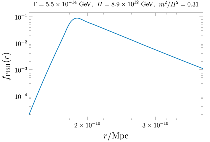
Figure 1 illustrates the typical shape of the function $f_{\rm PBH}(r)$ and the curvaton density parameter $\Omega_{\chi}$ at the horizon crossing of $r$, which enters in the computation via Eq. (3). The abundance $f_{\rm PBH}(r)$ has a clearly peaked structure although the curvaton spectrum Eq. (2.2) is of pure power law form. This is a generic feature in the setup and it arises from an interplay of two opposite effects. First, increasing the coarse-graining scale $r$ makes the variance $\sigma^{2}_{\chi\chi}(r)$ smaller, see Eq. (3.7), and therefore suppresses the probability of large $\chi(r)$ values that can source PBHs. Second, the curvature perturbation $\zeta$ and $\Omega_{\chi}$ keep growing in time until the curvaton decay at $H(t_{\rm dec})=\Gamma$. For $t_{\rm r}<(t_{\rm dec})$, increasing $r$ corresponds to later horizon crossing times $t_{\rm r}$, making $\zeta(t_{\rm r})$ larger and enhancing the probability for PBH formation. This effect dominates to the left of the $f_{\rm PBH}(r)$ peak in Fig. 1, and the peak corresponds to $t_{\rm r}=t_{\rm dec}$. To the right of the peak, $\zeta$ stays constant as $t_{\rm r}>t_{\rm dec}$. In this region, increasing $r$ only acts to decrease $\sigma^{2}_{\chi\chi}(r)$ and therefore $f_{\rm PBH}(r)$ starts to decrease. In the following, we will choose the coarse-graining scale $r$ equal to the peak scale by setting $r=r_{\rm dec}\equiv 1/(a(t_{\rm dec})H(t_{\rm dec}))$, and define $f_{\rm PBH}=f_{\rm PBH}(r_{\rm dec})$.

Figure 2: PBH abundance $f_{\rm PBH}$ as a function of the curvaton decay rate $\Gamma$ and the inflationary Hubble scale $H$. Computed for $m^{2}/H^{2}=0.31$ (left) and 0.35 (right).

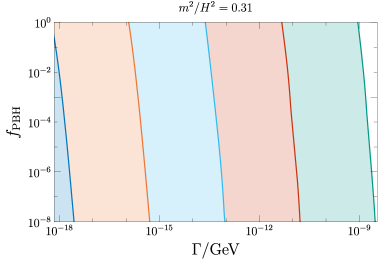
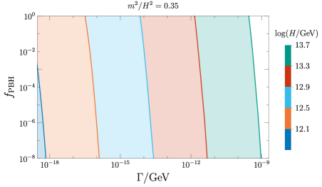
Figures 2 and 3 illustrate the behaviour of $f_{\rm PBH}$ as a function of the decay rate $\Gamma$, the inflationary Hubble scale $H$, and the curvaton mass parameter $m^{2}/H^{2}$. Varying the decay rate $\Gamma$ alters the curvaton density parameter $\Omega_{\chi}$ at $t_{\rm r}=t_{\rm dec}$. As seen in Fig. 1, $f_{\rm PBH}$ is a strongly dependent function of $\Omega_{\chi}$. Increasing $\Gamma$ moves the decay to earlier times and decreases $\Omega_{\chi}$ for fixed $H,m^{2}/H^{2}$ values. This explains the strong decrease of $f_{\rm PBH}$ as a function of $\Gamma$ in Figs. 2 and 3. The figures further show that, for a fixed $\Gamma$, increasing $m^{2}/H^{2}$ or decreasing $H$ causes $f_{\rm PBH}$ to decrease. The former is because larger $m^{2}/H^{2}$ makes the curvaton spectrum Eq. (2.2) more blue-tilted, decreasing the variance $\sigma_{\chi\chi}^{2}(r)$, Eq. (3.7), and therefore suppressing the probability for large $\chi(r)$ values. The latter is because the mean curvaton energy at the end of inflation $\langle\rho_{\chi}\rangle\propto m^{2}\langle\chi^{2}\rangle\propto H^{4}$ [66], and decreasing $H$ therefore decreases $\Omega_{\chi}$ for fixed $\Gamma$ and $m^{2}/H^{2}$ values.

Figure 3: PBH abundance $f_{\rm PBH}$ as a function of the curvaton decay rate $\Gamma$ and the curvaton mass parameter $m^{2}/H^{2}$. Computed for $H=8.9\times 10^{12}$ GeV.

The observational constraints on the PBH abundance $f_{\rm PBH}$ depend on the PBH mass which, setting $r=r_{\rm dec}$ in Eqs. (4.2) and (4.3), in our setup is parametrically proportional to

$$M_{\rm H}=4\pi M_{\rm P}^{2}\Gamma^{-1}\approx 1.3\times 10^{-15}M_{\odot}\left(\frac{\Gamma}{5\times 10^{-14}\;{\rm GeV}}\right)^{-1}~{}.$$ (5.1)

Black hole evaporation sets very strong constraints for PBHs with $M\lesssim 10^{-16}M_{\odot}$. Constraints for $M\gtrsim 10^{-10}M_{\odot}$ PBHs from various different systems range downwards from $f_{\rm PBH}={\cal O}(10^{-2})$ depending on the mass [4]. In the asteroid mass window $10^{-16}M_{\odot}\lesssim M\lesssim 10^{-10}M_{\odot}$, the constraints are subject to significant uncertainties and it can be possible to have $f_{\rm PBH}=1$ in this window [4]. Interestingly, asteroid mass PBHs can be efficiently produced in the curvaton scenario. This is demonstrated in Fig. 4 which shows the PBH mass spectra $f(M)$ computed using Eq. (4.7) for $\Gamma=5.5\times 10^{-18}$ GeV, $\Gamma=6.5\times 10^{-16}$ GeV and $\Gamma=5.5\times 10^{-14}$ GeV, with $m^{2}/H^{2}=0.31$, and $H$ chosen in each case such that $f_{\rm PBH}\approx 0.10$. The corresponding curvaton decay temperatures are $T_{\rm dec}\sim 2$ GeV for $\Gamma=5.5\times 10^{-18}$ GeV, $T_{\rm dec}\sim 20$ GeV for $\Gamma=6.5\times 10^{-16}$ GeV, and $T_{\rm dec}\sim 200$ GeV for $\Gamma=5.5\times 10^{-14}$ GeV, approximating the curvaton decay into radiation and the thermalisation of the decay products as instant processes, and using the Standard Model $g_{*}(T)$. The respective mass spectra in Fig. 4 are peaked at $M\sim 10^{-11}M_{\odot}$, $M\sim 10^{-13}M_{\odot}$ and $M\sim 10^{-15}M_{\odot}$. In all three cases, the PBH abundance can be increased by slightly increasing $H$, see Fig. 2. For example, $f_{\rm PBH}\approx 1.0$ is obtained with $H\approx 1.85\times 10^{12}$ GeV, $H\approx 4.25\times 10^{12}$ GeV, and $H\approx 9.19\times 10^{12}$ GeV for $\Gamma=5.5\times 10^{-18}$ GeV, $\Gamma=6.5\times 10^{-16}$ GeV, and $\Gamma=5.5\times 10^{-14}$ GeV, respectively.

Figure 4: The PBH mass distribution $f(M)$ normalised by the PBH abundance $f_{\rm PBH}$. In all figures $m^{2}/H^{2}=0.31$. The first panel shows the results for $\Gamma=5.5\times 10^{-18}$ GeV, $H\approx 1.78\times 10^{12}$ GeV, the second panel for $\Gamma=6.5\times 10^{-16}$ GeV, $H\approx 4.08\times 10^{12}$ GeV, and the third panel for $\Gamma=5.5\times 10^{-14}$ GeV, $H\approx 8.85\times 10^{12}$ GeV. In all cases $f_{\rm PBH}\approx 0.10$.

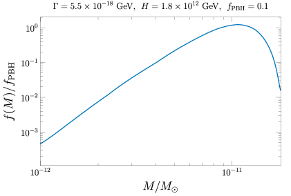
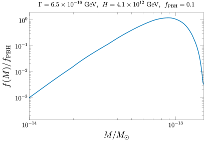
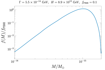
Figures 2, 3 and 4 represent the main results of this work. In particular, they show that the curvaton scenario can generate a significant dark matter fraction consisting of asteroid mass scale PBHs when the inflationary Hubble scale is large enough $H\gtrsim 10^{12}$ GeV, the curvaton mass parameter $m^{2}/H^{2}\gtrsim 0.3$ and the decay rate falls in the window $10^{-18}\;{\rm GeV}\lesssim\Gamma\lesssim 10^{-13}$ GeV, corresponding to decay temperatures from slightly above the electroweak transition to around the QCD transition scale. If the curvaton decay occurs earlier, $10^{-13}\;{\rm GeV}\lesssim\Gamma\lesssim 10^{-8}\;{\rm GeV}$, the scenario generates PBHs with $M\lesssim 10^{-16}M_{\odot}$ and, according to the dependencies shown in Figs. 2 and 3, the observational constraints on $f_{\rm PBH}$ constrains the viable parameter space for $H$ from above and for $m^{2}/H^{2}$ from below. For $\Gamma\gtrsim 10^{-8}\;{\rm GeV}$ there are no constraints as the PBH abundance is exponentially suppressed for any $H\lesssim 5.2\times 10^{13}$ GeV compatible with the observational bound on the tensor-to-scalar ratio $r_{\rm T}<0.044$ [80], and $m^{2}/H^{2}$ in the range compatible with Eq. (2.10). For $\Gamma\lesssim 10^{-18}\;{\rm GeV}$, the scenario generates PBHs with $M\gtrsim 10^{-10}M_{\odot}$ but in this region our numerical integration of Eq. (3) starts to become inaccurate for configurations leading to $f_{\rm PBH}\gtrsim 0.01$. We are therefore not able to perform a detailed study of the $\Gamma\lesssim 10^{-18}\;{\rm GeV}$ region in this work.

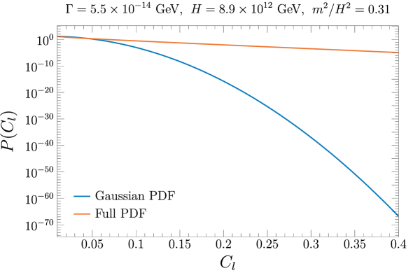
Finally, Fig. 5 depicts the probability distribution $P_{C_{l}}(C_{l},r_{\rm dec})$ given by Eq. (3) for the same choice of parameters as in Fig. 1, and in the third panel of Fig. 4. For comparison, we also show a Gaussian distribution with the variance equal to the variance computed from the full distribution for this set of parameters, $\int\mathrm{d}C_{l}\ C_{l}^{2}P_{C_{l}}(C_{l},r_{\rm dec})\approx 5.1\times 10^{-4}$. The full distribution deviates significantly from the Gaussian case and decays much slower as a function of $C_{l}$. The slowly decaying tail of $P_{C_{l}}(C_{l},r_{\rm dec})$ is essential for the PBH formation in our setup. We recall, that the fully non-Gaussian form of $P_{C_{l}}(C_{l},r_{\rm dec})$ follows from the vanishing mean of the curvaton field $\langle\chi\rangle=0$ which in turn is the equilibrium configuration during inflation for the $\chi^{2}$ potential. The curvature perturbation component $\zeta_{\chi}\propto{\rm ln}\rho_{\chi}/\langle\rho_{\chi}\rangle={\rm ln}\chi^{2}/\langle\chi^{2}\rangle$ has no leading Gaussian term and there is no suppression for fluctuations $\chi^{2}/\langle\chi^{2}\rangle\sim 1$. Together with the non-linear form of Eq. (2.7), this gives rise to the strongly non-Gaussian distribution of $C_{l}$ seen in Fig. 5.

Figure 5: The full probability distribution function $P_{C_{l}}(C_{l},r_{\rm dec})$ and a Gaussian distribution with the same variance $\langle C_{l}^{2}\rangle\approx 5.1\times 10^{-4}$. Parameters chosen as in Fig. 1.

6 Summary

In this work we have investigated the PBH production in the mixed inflaton–curvaton scenario with a quadratic curvaton potential and a strongly blue-tilted curvaton spectrum, assuming the curvaton is in the de Sitter equilibrium $\langle\chi\rangle=0$ during inflation. We require that the inflaton sourced Gaussian component dominates the spectrum of the curvature perturbation $\zeta$ on CMB scales and the curvaton sourced contribution is suppressed below the $2\times 10^{-11}$ level at the pivot scale $k_{*}=0.05\ {\rm Mpc}^{-1}$. This constrains the curvaton mass from below, for example for the inflationary Hubble scale $H=10^{13}$ GeV, the curvaton mass must satisfy $m^{2}/H^{2}\gtrsim 0.3$. On small scales, however, the curvaton sourced component of $\zeta$ can take large values leading to PBH formation.

A key feature in this setup, is that the curvaton sourced part of $\zeta$ is strongly non-Gaussian. It contains no leading Gaussian term, unlike in scenarios with a non-vanishing curvaton mean value $|\langle\chi\rangle|\gg H$ (a specific initial condition during inflation) which have been studied previously in the PBH context e.g. in [47, 48, 49, 50, 51]. We use the $\delta N$ formalism to obtain the full non-linear solution for $\zeta$ as a function of $\chi$ and, following [63], include only the monopole term of the spherical harmonics series of $\chi({\bf x})$ when considering fluctuations relevant for PBHs. With this approximation, we compute the probability distribution for $C_{l}(r)$ which determines the compaction function $C(C_{l}(r))$, and where $r$ is the coarse-graining scale of perturbations. Comparing to a fiducial Gaussian distribution with the same variance $\langle C_{l}^{2}\rangle$, we find that the full distribution $P_{l}(C_{l},r)$ decreases exponentially slower as a function of $C_{l}$. We use $C_{\rm c}=0.55$ as the threshold for the PBH collapse [75] and model the PBH mass with parameters obtained for the power-law spectrum in [74, 75].

We find that the curvaton scenario with $\langle\chi\rangle=0$ can lead to very efficient production of PBHs. In particular, the setup can generate asteroid mass PBHs, $10^{-16}M_{\odot}\lesssim M\lesssim 10^{-10}M_{\odot}$, with an abundance equal to the observed dark matter abundance, $f_{\rm PBH}=1$, when the Hubble scale at the end of inflation $H\gtrsim 10^{12}$ GeV, the curvaton mass $m^{2}/H^{2}\gtrsim 0.3$ and the curvaton decay occurs in the window from slightly before the electroweak transition to around the QCD transition. If the curvaton decays before or after the aforementioned window, PBHs with masses below or above the asteroid mass range can be generated, respectively. The PBH abundance depends sensitively on $H$, $m^{2}/H^{2}$ and the curvaton decay rate $\Gamma$, and the observational bounds on $f_{\rm PBH}$ imply non-trivial constraints on these parameters when $\Gamma\lesssim 10^{-8}$ GeV. For larger values of $\Gamma$ the PBH production in the setup is exponentially suppressed.

The main uncertainties in our results arise from the monopole truncation Eq. (3.5) and the phenomenological choice of collapse parameters in Eq. (4.2). Changing the collapse parameter values would affect $f_{\rm PBH}$ predicted for a fixed set of curvaton parameters. However, even order of magnitude changes of $f_{\rm PBH}$ are compensated by just slight changes of $H$, $m^{2}/H^{2}$ and $\Gamma$, as can be seen in Figs. 2 and 3. The error caused by the use of Eq. (3.5) is harder to quantify but we expect that the very efficient PBH production from the strongly non-Gaussian $\zeta$ is a robust conclusion.

Appendix A The spectrum of $\zeta_{\chi}$

We use the stochastic formalism [66] and the spectral expansion method [95, 96, 97] to compute the infrared spectrum of $\zeta_{\chi}$ in our setup where $\langle\chi\rangle=0$ and Eq. (2.6) cannot be expanded in small perturbations around a mean field. For the quadratic curvaton potential (2.1), the joint equal time two-point distribution of $\chi(t,{\bf r})$ in de Sitter equilibrium is given by the spectral sum [95, 96, 97]

$$\rho_{2}(\chi,{\bf r},t;\chi^{\prime},{\bf r}^{\prime},t)=\frac{m^{2}}{H^{4}}\psi_{0}(x)\psi_{0}(x^{\prime})\sum_{n=0}^{\infty}\psi_{n}(x)\psi_{n}(x^{\prime})\left(a(t)H|{\bf r}-{\bf r}^{\prime}|\right)^{-2\Lambda_{n}/H}\;,$$ (A.1)

where

$$x=\frac{m\chi}{H^{2}}\;,\quad\Lambda_{n}=\frac{nm^{2}}{3H}\;,\quad\psi_{n}(x)=\frac{1}{\sqrt{n!2^{n}}}\left(\frac{4\pi}{3}\right)^{1/4}e^{-2\pi^{2}x^{2}/3}H_{n}\left(\frac{2\pi x}{\sqrt{3}}\right)\;,$$ (A.2)

and $H_{n}(x)=(-1)^{n}e^{x^{2}/2}\frac{\mathrm{d}^{n}}{\mathrm{d}x^{n}}e^{-x^{2}/2}$ are the Hermite polynomials. The eigenfunctions $\psi_{n}(x)$ are orthonormal,

$$\int_{-\infty}^{\infty}\mathrm{d}x\ \psi_{m}(x)\psi_{n}(x)=\delta_{mn}\;.$$ (A.3)

Using that $\langle\chi^{2}\rangle={3H^{4}}/({8\pi^{2}m^{2}})$, we have from Eq. (2.6) $\zeta_{\chi}=(1/3){\rm ln}(8\pi^{3}x^{2}/3)$, and the connected part of its two-point function can be written as

$$\langle{\zeta}_{\chi}({\bf r}){\zeta}_{\chi}({\bf r}^{\prime})\rangle_{\rm c} = \int_{-\infty}^{\infty}\mathrm{d}\chi\int_{-\infty}^{\infty}\mathrm{d}\chi^{\prime}\ {\zeta}(\chi){\zeta}(\chi^{\prime})\rho_{2}(\chi,{\bf r},t;\chi^{\prime},{\bf r}^{\prime},t)$$ (A.4)

$$= \sum_{n=1}^{\infty}\left(\int_{-\infty}^{\infty}\mathrm{d}x\ \frac{1}{3}\psi_{0}(x)\psi_{n}(x)\ln{x}^{2}\right)^{2}\left(a(t)H|\textbf{r}-\textbf{r}^{\prime}|\right)^{-\frac{2nm^{2}}{3H^{2}}}\;.$$

Truncating the series at the leading order we get

$$\langle{\zeta}_{\chi}({\bf r}){\zeta}_{\chi}({\bf r}^{\prime})\rangle_{\rm c}=\frac{2}{9}\left(aH|{\bf r}-{\bf r}^{\prime}|\right)^{-\frac{4m^{2}}{3H^{2}}}+\mathcal{O}\left[\left(aH|{\bf r}-{\bf r}^{\prime}|\right)^{-\frac{8m^{2}}{3H^{2}}}\right]\;.$$ (A.5)

The corresponding power spectrum is given by

$${\cal P}_{\zeta_{\chi}} = \frac{k^{3}}{2\pi^{2}}\int\mathrm{d}^{3}r\ e^{-i\textbf{k}\cdot\textbf{r}}\langle{\zeta}_{\chi}({\bf r}){\zeta}_{\chi}({\bf r}^{\prime})\rangle_{\rm c}$$ (A.6)

$$= \frac{2^{3-\frac{4m^{2}}{3H^{2}}}}{9\sqrt{\pi}}\frac{\Gamma\left(\frac{3}{2}-\frac{2m^{2}}{3H^{2}}\right)}{\Gamma\left(\frac{2m^{2}}{3H^{2}}\right)}\left(\frac{k}{aH}\right)^{\frac{4m^{2}}{3H^{2}}}\;.$$

The existence of the Fourier transform requires $4m^{2}<9H^{2}$ which we assume here.

Assuming an instant transition from de Sitter inflation to radiation dominated epoch, and approximating the universe as radiation dominated until the curvaton decay, we can write

$$\frac{k}{aH}=6\times 10^{-24}\frac{k}{0.05\ {\rm Mpc}^{-1}}\frac{10^{15}{\rm GeV}}{\rho^{1/4}}~{},$$ (A.7)

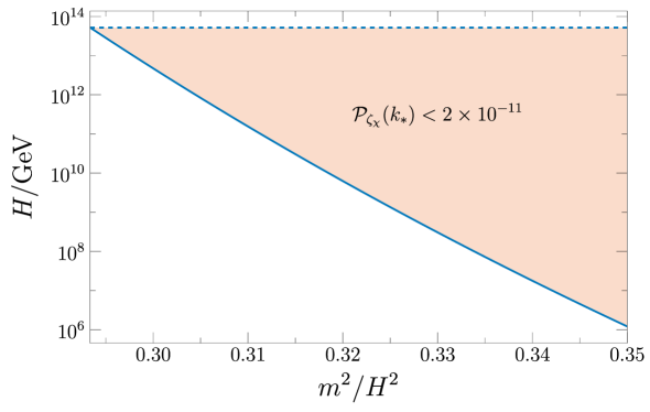
where $\rho=3H^{2}M_{\rm P}^{2}$ denotes the energy density during inflation. Using Eqs. (A.6) and (A.7) we can directly solve for the $m^{2}/H^{2}$ range where the condition Eq. (2.10) is satisfied, i.e. ${\cal P}_{\zeta_{\chi}}(k_{*})<2\times 10^{-11}$. The result is shown in Fig. 6 where the shaded orange area marks the region where Eq. (2.10) holds.

Figure 6: Above the solid line ${\cal P}_{\zeta_{\chi}}(k_{*})<2\times 10^{-11}$. The dashed line shows the maximum inflationary Hubble scale $H\approx 5.2\times 10^{13}\;{\rm GeV}$ consistent with the observational bound on the tensor-to-scalar ratio $r_{\rm T}<0.044$ [80]. The shaded orange area between the solid and dashed lines depicts the phenomenologically viable region where ${\cal P}_{\zeta_{\chi}}(k_{*})<2\times 10^{-11}$.

We will also need the two point functions of the powers $\zeta^{\ell}_{\chi}$ in the analysis below. These can be directly computed using the spectral expansion expression

$$\langle{\zeta}_{\chi}^{{\ell}}({\bf r}){\zeta}_{\chi}^{{\ell}^{\prime}}({\bf r}^{\prime})\rangle_{\rm c} = \int_{-\infty}^{\infty}\mathrm{d}\chi\int_{-\infty}^{\infty}\mathrm{d}\chi^{\prime}\ {\zeta}^{\ell}(\chi){\zeta}^{\ell^{\prime}}(\chi^{\prime})\rho_{2}(\chi,{\bf r},t;\chi^{\prime},{\bf r}^{\prime},t)$$

$$= \sum_{n=1}^{\infty}\sum_{n^{\prime}=1}^{\infty}\left(\int_{-\infty}^{\infty}\mathrm{d}x\ \frac{1}{3}\psi_{0}(x)\psi_{n}(x)\ln{x}^{2}\right)^{{\ell}}\left(\int_{-\infty}^{\infty}\mathrm{d}x^{\prime}\ \frac{1}{3}\psi_{0}(x^{\prime})\psi_{n}(x^{\prime})\ln{x^{\prime}}^{2}\right)^{{\ell}^{\prime}}\times$$

$$\left(a(t)H|\textbf{r}-\textbf{r}^{\prime}|\right)^{-\frac{2(n+n^{\prime})m^{2}}{3H^{2}}}~{}.$$

Truncating the series again at the leading order we obtain

$$\langle{\zeta}_{\chi}^{{\ell}}({\bf r}){\zeta}_{\chi}^{{\ell}^{\prime}}({\bf r}^{\prime})\rangle_{\rm c}=\left(\frac{\sqrt{2}}{3}\right)^{\ell+\ell^{\prime}}\left(aH|{\bf r}-{\bf r}^{\prime}|\right)^{-\frac{4m^{2}}{3H^{2}}}+\mathcal{O}\left[\left(aH|{\bf r}-{\bf r}^{\prime}|\right)^{-\frac{8m^{2}}{3H^{2}}}\right]~{}.$$ (A.9)

Appendix B The spectrum of $\zeta$ on CMB scales

We express the full solution Eq. (2.7) for $\zeta$ in the form

$$\zeta=\zeta_{\rm r}+Z(\zeta_{\chi},\zeta_{\rm r})~{},$$ (B.1)

where the explicit expression for $Z(\zeta_{\chi},\zeta_{\rm r})$ can be read off from Eq. (2.7). The connected part of the two point function of $\zeta$ is given by

$$\langle\zeta({\bf r})\zeta({\bf r}^{\prime})\rangle_{\rm c}=\langle\zeta_{\rm r}({\bf r})\zeta_{\rm r}({\bf r}^{\prime})\rangle_{\rm c}+2\langle Z({\bf r})\zeta_{\rm r}({\bf r}^{\prime})\rangle_{\rm c}+\langle Z({\bf r})Z({\bf r}^{\prime})\rangle_{\rm c}~{}.$$ (B.2)

Expanding $Z(\zeta_{\chi}-\zeta_{\rm r})$ around $\zeta_{\rm r}=0$, the last two terms can be written as

$$\langle Z({\bf r})\zeta_{\rm r}({\bf r}^{\prime})\rangle_{\rm c} = \sum_{n=0}^{\infty}\frac{1}{(2n+1)!}\langle Z^{(2n+1)}(\zeta_{\chi})\rangle\langle\zeta_{\rm r}({\bf r})\zeta_{\rm r}^{2n+1}({\bf r}^{\prime})\rangle_{\rm c}$$ (B.3)

$$\langle Z({\bf r})Z({\bf r}^{\prime})\rangle_{\rm c} = \sum_{n=1}^{\infty}\sum_{n^{\prime}=1}^{\infty}\frac{1}{n!n^{\prime}!}\langle Z^{(n)}(\zeta_{\chi})\rangle\langle Z^{(n^{\prime})}(\zeta_{\chi})\rangle\langle\zeta_{\rm r}^{n}({\bf r})\zeta_{\rm r}^{n^{\prime}}({\bf r}^{\prime})\rangle_{\rm c}$$

$$+{~{}\rm terms~{}involving~{}}\langle\zeta_{\chi}^{n}({\bf r})\zeta_{\chi}^{n^{\prime}}({\bf r}^{\prime})\rangle_{\rm c}~{}.$$

We assume the curvature perturbation of the radiation component is sourced by the inflaton, and is Gaussian distributed with a nearly scale invariant spectrum

$${\cal P}_{\zeta_{\rm r}}(k)=A_{\rm r}\left(\frac{k}{k_{*}}\right)^{n_{\rm r}-1}~{},\qquad A_{\rm r}\gg P_{\zeta_{\chi}}(k_{*})~{},$$ (B.5)

and require that the curvaton component is suppressed on CMB scales such that $P_{\zeta_{\chi}}(k_{*})<2\times 10^{-11}$ according to Eq. (2.10). Using Eq. (A.9), we then observe that on scales $k\lesssim k_{*}$ we can to leading precision drop all terms involving connected correlators of $\zeta_{\chi}^{n}$ in Eq. (B). On scales $k\lesssim k_{*}$, the leading contribution to the two point function Eq. (B.2) then reads

$$\langle\zeta({\bf r})\zeta({\bf r}^{\prime})\rangle_{\rm c}\approx\langle\zeta_{\rm r}({\bf r})\zeta_{\rm r}({\bf r}^{\prime})\rangle_{\rm c}\left(1+\left\langle Z^{(1)}(\zeta_{\chi})\right\rangle\right)^{2}~{}.$$ (B.6)

The non-linear function $\langle Z^{(1)}(\zeta_{\chi})\rangle$ involves contributions from closed $\zeta_{\chi}$ loops attached to the points ${\bf r}$ or ${\bf r}^{\prime}$. Since $\langle Z^{(1)}(\zeta_{\chi})\rangle$ has no dependence on spatial coordinates, the spectrum of the curvature perturbation for $k\lesssim k_{*}$ is simply given by

$${\cal P}_{\zeta}(k)=A\left(\frac{k}{k_{*}}\right)^{n_{\rm r}}~{},\qquad A=A_{\rm r}\left(1+\left\langle Z^{(1)}(\zeta_{\chi})\right\rangle\right)^{2}~{},\qquad k\lesssim k_{*}~{}.$$ (B.7)

Figure 7: The solid line shows $A/A_{\rm r}$ defined in Eq. (B.7) as a function of the curvaton density parameter $\Omega_{\chi}$. The dashed line shows the corresponding quantity computed in linear perturbation theory.

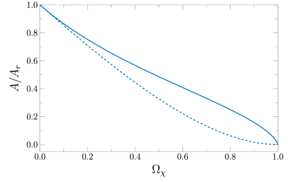
Figure 7 shows the ratio $A/A_{\rm r}$ as function of $\Omega_{\chi}$. For comparison, we have also plotted the corresponding linear perturbation theory result $A/A_{\rm r}=(4(1-\Omega_{\chi})/(4-\Omega))^{2}$ obtained from $\zeta=4\zeta_{\rm r}(1-\Omega_{\chi})/(4-\Omega)+3\zeta_{\chi}\Omega_{\chi}/(4-\Omega)$, see e.g. [98], when ${\cal P}_{\zeta_{\chi}}(k)\ll{\cal P}_{\zeta_{\rm r}}(k)$. As seen in Fig. 7, for $\Omega_{\chi}\lesssim 0.9$ we have $0.2\lesssim A/A_{\rm r}\leqslant 1$, indicating that the observed CMB spectrum amplitude ${\cal P}_{\zeta}(k_{*})=A=2.10\times 10^{-9}$ is obtained by adjusting the inflaton sector to give $A_{\rm r}$ in the range $5\gtrsim A_{\rm r}\geqslant 1$, correspondingly. From Eqs. (A.9) and (B.2)–(B) we further see that when Eq. (2.10) holds, the contributions from $\zeta_{\chi}$ to the spectral index $n_{\rm s}-1=\mathrm{d}{\rm ln}P_{\zeta}/\mathrm{d}{\rm ln}k$ are parametrically suppressed to ${\cal O}(0.01)$. The measured spectral index $n_{\rm s}=0.965$ at $k=k_{*}$ should then be obtainable with slow roll inflationary models having $\epsilon={\cal O}(0.01)$ which can be adjusted to give the correct $n_{\rm s}$. We thus conclude that when Eq. (2.10) holds, we obtain inflaton dominated, Gaussian and nearly scale-invariant perturbations on CMB scales.

References

- [1] Ya. B. Zel’dovich and I. D. Novikov, The Hypothesis of Cores Retarded during Expansion and the Hot Cosmological Model, Soviet Astronomy 10(4) (1967) 602.
- [2] S. Hawking, Gravitationally Collapsed Objects of Very Low Mass, Monthly Notices of the Royal Astronomical Society 152(1) (1971) 75.
- [3] G. F. Chapline, Cosmological effects of primordial black holes, Nature 253(5489) (1975) 251.
- [4] B. Carr, K. Kohri, Y. Sendouda and J. Yokoyama, Constraints on primordial black holes, Reports on Progress in Physics 84(11) (2021) 116902 [2002.12778].
- [5] S. Bird et al., Did LIGO detect dark matter?, Physical Review Letters 116(20) (2016) 201301 [1603.00464].
- [6] S. Clesse and J. García-Bellido, The clustering of massive Primordial Black Holes as Dark Matter: measuring their mass distribution with Advanced LIGO, Physics of the Dark Universe 15 (2017) 142 [1603.05234].
- [7] M. Sasaki, T. Suyama, T. Tanaka and S. Yokoyama, Primordial Black Hole Scenario for the Gravitational-Wave Event GW150914, Physical Review Letters 117(6) (2016) 061101 [1603.08338].
- [8] A. D. Gow, C. T. Byrnes, A. Hall and J. A. Peacock, Primordial black hole merger rates: distributions for multiple LIGO observables, Journal of Cosmology and Astroparticle Physics 2020(01) (2020) 031 [1911.12685].
- [9] G. Franciolini et al., Searching for a subpopulation of primordial black holes in LIGO-Virgo gravitational-wave data, Physical Review D 105(8) (2022) 083526 [2105.03349].
- [10] P. Ivanov, P. Naselsky and I. Novikov, Inflation and primordial black holes as dark matter, Physical Review D 50(12) (1994) 7173.
- [11] J. García-Bellido, A. Linde and D. Wands, Density perturbations and black hole formation in hybrid inflation, Physical Review D 54(10) (1996) 6040 [astro-ph/9605094].
- [12] P. Ivanov, Nonlinear metric perturbations and production of primordial black holes, Physical Review D 57(12) (1998) 7145 [astro-ph/9708224].
- [13] S. M. Leach, I. J. Grivell and A. R. Liddle, Black hole constraints on the running mass inflation model, Physical Review D 62(4) (2000) 043516 [astro-ph/0004296].
- [14] M. Drees and E. Erfani, Running-mass inflation model and primordial black holes, Journal of Cosmology and Astroparticle Physics 2011(04) (2011) 005 [1102.2340].
- [15] M. Drees and E. Erfani, Running spectral index and formation of primordial black hole in single field inflation models, Journal of Cosmology and Astroparticle Physics 2012(01) (2012) 035 [1110.6052].
- [16] J. García-Bellido and E. Ruiz Morales, Primordial black holes from single field models of inflation, Physics of the Dark Universe 18 (2017) 47 [1702.03901].
- [17] V. Domcke, F. Muia, M. Pieroni and L. T. Witkowski, PBH dark matter from axion inflation, Journal of Cosmology and Astroparticle Physics 2017(07) (2017) 048 [1704.03464].
- [18] K. Kannike, L. Marzola, M. Raidal and H. Veermäe, Single field double inflation and primordial black holes, Journal of Cosmology and Astroparticle Physics 2017(09) (2017) 020 [1705.06225].
- [19] C. Germani and T. Prokopec, On primordial black holes from an inflection point, Physics of the Dark Universe 18 (2017) 6 [1706.04226].
- [20] H. Motohashi and W. Hu, Primordial black holes and slow-roll violation, Physical Review D 96(6) (2017) 063503 [1706.06784].
- [21] G. Ballesteros and M. Taoso, Primordial black hole dark matter from single field inflation, Physical Review D 97(2) (2018) 023501 [1709.05565].
- [22] M. P. Hertzberg and M. Yamada, Primordial Black Holes from Polynomial Potentials in Single Field Inflation, Physical Review D 97(8) (2018) 083509 [1712.09750].
- [23] S. Pi, Y.-l. Zhang, Q.-G. Huang and M. Sasaki, Scalaron from -gravity as a heavy field, Journal of Cosmology and Astroparticle Physics 2018(05) (2018) 042 [1712.09896].
- [24] K. Kohri and T. Terada, Primordial black hole dark matter and LIGO/Virgo merger rate from inflation with running spectral indices: formation in the matter- and/or radiation-dominated universe, Classical and Quantum Gravity 35(23) (2018) 235017 [1802.06785].
- [25] M. Biagetti, G. Franciolini, A. Kehagias and A. Riotto, Primordial black holes from inflation and quantum diffusion, Journal of Cosmology and Astroparticle Physics 2018(07) (2018) 032 [1804.07124].
- [26] I. Dalianis, A. Kehagias and G. Tringas, Primordial black holes from -attractors, Journal of Cosmology and Astroparticle Physics 2019(01) (2019) 037 [1805.09483].
- [27] G. Ballesteros, J. Beltrán Jiménez and M. Pieroni, Black hole formation from a general quadratic action for inflationary primordial fluctuations, Journal of Cosmology and Astroparticle Physics 2019(06) (2019) 016 [1811.03065].
- [28] J. Georg, B. Melcher and S. Watson, Primordial black holes and Co-Decaying dark matter, Journal of Cosmology and Astroparticle Physics 2019(11) (2019) 014 [1902.04082].
- [29] S. Pi, M. Sasaki and Y.-l. Zhang, Primordial tensor perturbation in double inflationary scenario with a break, Journal of Cosmology and Astroparticle Physics 2019(06) (2019) 049 [1904.06304].
- [30] C. Germani and I. Musco, Abundance of Primordial Black Holes Depends on the Shape of the Inflationary Power Spectrum, Physical Review Letters 122(14) (2019) 141302 [1805.04087].
- [31] B. Carr and F. Kühnel, Primordial black holes with multimodal mass spectra, Physical Review D 99(10) (2019) 103535 [1811.06532].
- [32] A. Y. Kamenshchik, A. Tronconi, T. Vardanyan and G. Venturi, Non-canonical inflation and primordial black holes production, Physics Letters B 791 (2019) 201 [1812.02547].
- [33] S. W. Hawking, Black holes from cosmic strings, Physics Letters B 231(3) (1989) 237.
- [34] J. Garriga and M. Sakellariadou, Effects of friction on cosmic strings, Physical Review D 48(6) (1993) 2502 [hep-th/9303024].
- [35] R. R. Caldwell and P. Casper, Formation of black holes from collapsed cosmic string loops, Physical Review D 53(6) (1996) 3002 [gr-qc/9509012].
- [36] K. Jedamzik, Primordial black hole formation during the QCD epoch, Physical Review D 55(10) (1997) 5871 [astro-ph/9605152].
- [37] C. T. Byrnes, M. Hindmarsh, S. Young and M. R. S. Hawkins, Primordial black holes with an accurate QCD equation of state, Journal of Cosmology and Astroparticle Physics 2018(08) (2018) 041 [1801.06138].
- [38] A. Chakraborty, P. K. Chanda, K. L. Pandey and S. Das, Formation and Abundance of Late-forming Primordial Black Holes as Dark Matter, The Astrophysical Journal 932(2) (2022) 119 [2204.09628].
- [39] S. Shandera, D. Jeong and H. S. Grasshorn Gebhardt, Gravitational Waves from Binary Mergers of Subsolar Mass Dark Black Holes, Physical Review Letters 120(24) (2018) 241102 [1802.08206].
- [40] J.-W. Chen, J. Liu, H.-L. Xu and Y.-F. Cai, Tracing primordial black holes in nonsingular bouncing cosmology, Physics Letters B 769 (2017) 561 [1609.02571].
- [41] J. Quintin and R. H. Brandenberger, Black hole formation in a contracting universe, Journal of Cosmology and Astroparticle Physics 2016(11) (2016) 029 [1609.02556].
- [42] D. H. Lyth and D. Wands, Generating the curvature perturbation without an inflaton, Physics Letters B 524(1–2) (2002) 5 [hep-ph/0110002].
- [43] T. Moroi and T. Takahashi, Effects of cosmological moduli fields on cosmic microwave background, Physics Letters B 522(3–4) (2001) 215 [hep-ph/0110096].
- [44] K. Enqvist and M. S. Sloth, Adiabatic CMB perturbations in pre-Big Bang string cosmology, Nuclear Physics B 626(1–2) (2002) 395 [hep-ph/0109214].
- [45] A. Linde and V. Mukhanov, Non-Gaussian isocurvature perturbations from inflation, Physical Review D 56(2) (1997) 535 [astro-ph/9610219].
- [46] S. Mollerach, Isocurvature baryon perturbations and inflation, Physical Review D 42(2) (1990) 313.
- [47] P. A. Klimai and E. V. Bugaev, Primordial black hole formation from non-Gaussian curvature perturbations, in Proc. of 17th Int. Seminar QUARKS-2012, vol. 2, p. 163, 2013, 1210.3262.
- [48] S. Young and C. T. Byrnes, Primordial black holes in non-Gaussian regimes, Journal of Cosmology and Astroparticle Physics 2013(08) (2013) 052 [1307.4995].
- [49] M. Kawasaki, N. Kitajima and T. T. Yanagida, Primordial black hole formation from an axionlike curvaton model, Physical Review D 87(6) (2013) 063519 [1207.2550].
- [50] S. Pi and M. Sasaki, Primordial Black Hole Formation in Non-Minimal Curvaton Scenario, (2021) [2112.12680].
- [51] D.-S. Meng, C. Yuan and Q.-G. Huang, Primordial black holes generated by the non-minimal spectator field, Science China Physics, Mechanics & Astronomy 66(8) (2023) 280411 [2212.03577].
- [52] B. Carr, F. Kühnel and M. Sandstad, Primordial black holes as dark matter, Physical Review D 94(8) (2016) 083504 [1607.06077].
- [53] J. García-Bellido, M. Peloso and C. Unal, Gravitational waves at interferometer scales and primordial black holes in axion inflation, Journal of Cosmology and Astroparticle Physics 2016(12) (2016) 031 [1610.03763].
- [54] B. Carr, T. Tenkanen and V. Vaskonen, Primordial black holes from inflaton and spectator field perturbations in a matter-dominated era, Physical Review D 96(6) (2017) 063507 [1706.03746].
- [55] J. M. Ezquiaga, J. García-Bellido and E. Ruiz Morales, Primordial black hole production in Critical Higgs Inflation, Physics Letters B 776 (2018) 345 [1705.04861].
- [56] J. R. Espinosa, D. Racco and A. Riotto, Cosmological Signature of the Standard Model Higgs Vacuum Instability: Primordial Black Holes as Dark Matter, Physical Review Letters 120(12) (2018) 121301 [1710.11196].
- [57] A. Cable and A. Wilkins, Spectators no more! How even unimportant fields can ruin your Primordial Black Hole model, (2023) [2306.09232].
- [58] J. S. Bullock and J. R. Primack, Non-Gaussian fluctuations and primordial black holes from inflation, Physical Review D 55(12) (1997) 7423 [astro-ph/9611106].
- [59] S. Young, D. Regan and C. T. Byrnes, Influence of large local and non-local bispectra on primordial black hole abundance, Journal of Cosmology and Astroparticle Physics 2016(02) (2016) 029 [1512.07224].
- [60] C.-M. Yoo, J.-O. Gong and S. Yokoyama, Abundance of primordial black holes with local non-Gaussianity in peak theory, Journal of Cosmology and Astroparticle Physics 2019(09) (2019) 033 [1906.06790].
- [61] M. Taoso and A. Urbano, Non-gaussianities for primordial black hole formation, Journal of Cosmology and Astroparticle Physics 2021(08) (2021) 016 [2102.03610].
- [62] S. Young, Peaks and primordial black holes: the effect of non-Gaussianity, Journal of Cosmology and Astroparticle Physics 2022(05) (2022) 037 [2201.13345].
- [63] A. D. Gow et al., Non-perturbative non-Gaussianity and primordial black holes, Europhysics Letters 142(4) (2023) 49001 [2211.08348].
- [64] G. Ferrante, G. Franciolini, A. J. Iovino and A. Urbano, Primordial non-Gaussianity up to all orders: Theoretical aspects and implications for primordial black hole models, Physical Review D 107(4) (2023) 043520 [2211.01728].
- [65] G. Ferrante, G. Franciolini, A. J. Iovino and A. Urbano, Primordial black holes in the curvaton model: possible connections to pulsar timing arrays and dark matter, (2023) [2305.13382].
- [66] A. A. Starobinsky and J. Yokoyama, Equilibrium state of a self-interacting scalar field in the de Sitter background, Physical Review D 50(10) (1994) 6357 [astro-ph/9407016].
- [67] K. Enqvist, R. N. Lerner, O. Taanila and A. Tranberg, Spectator field dynamics in de Sitter and curvaton initial conditions, Journal of Cosmology and Astroparticle Physics 2012(10) (2012) 052 [1205.5446].
- [68] R. J. Hardwick et al., The stochastic spectator, Journal of Cosmology and Astroparticle Physics 2017(10) (2017) 018 [1701.06473].
- [69] Planck collaboration, Planck 2018 results. IX. Constraints on primordial non-Gaussianity, Astronomy & Astrophysics 641 (2020) A9 [1905.05697].
- [70] A. A. Starobinsky, Multicomponent de Sitter (inflationary) stages and the generation of perturbations, Journal of Experimental and Theoretical Physics Letters 42(3) (1985) 124.
- [71] D. S. Salopek and J. R. Bond, Nonlinear evolution of long-wavelength metric fluctuations in inflationary models, Physical Review D 42(12) (1990) 3936.
- [72] M. Sasaki and E. D. Stewart, A General Analytic Formula for the Spectral Index of the Density Perturbations Produced during Inflation, Progress of Theoretical Physics 95(1) (1996) 71 [astro-ph/9507001].
- [73] D. Wands, K. A. Malik, D. H. Lyth and A. R. Liddle, New approach to the evolution of cosmological perturbations on large scales, Physical Review D 62(4) (2000) 043527 [astro-ph/0003278].
- [74] I. Musco, J. C. Miller and A. G. Polnarev, Primordial black hole formation in the radiative era: investigation of the critical nature of the collapse, Classical and Quantum Gravity 26(3) (2009) 235001 [0811.1452].
- [75] I. Musco, V. De Luca, G. Franciolini and A. Riotto, Threshold for primordial black holes. II. A simple analytic prescription, Physical Review D 103(6) (2021) 063538 [2011.03014].
- [76] R. Ebadi et al., Gravitational Waves from Stochastic Scalar Fluctuations, (2023) [2307.01248].
- [77] T. S. Bunch and P. C. W. Davies, Quantum field theory in de Sitter space: renormalization by point splitting, Proceedings of the Royal Society A 360(1700) (1978) 117.
- [78] M. Sasaki, J. Väliviita and D. Wands, Non-Gaussianity of the primordial perturbation in the curvaton model, Physical Review D 74(10) (2006) 103003 [astro-ph/0607627].
- [79] Planck collaboration, Planck 2018 results. VI. Cosmological parameters, Astronomy & Astrophysics 641 (2020) A6 [1807.06209].
- [80] M. Tristram et al., Planck constraints on the tensor-to-scalar ratio, Astronomy & Astrophysics 647 (2021) A128 [2010.01139].
- [81] M. Shibata and M. Sasaki, Black hole formation in the Friedmann universe: Formulation and computation in numerical relativity, Physical Review D 60(8) (1999) 084002 [gr-qc/9905064].
- [82] T. Harada, C.-M. Yoo, T. Nakama and Y. Koga, Cosmological long-wavelength solutions and primordial black hole formation, Physical Review D 91(8) (2015) 084057 [1503.03934].
- [83] C.-M. Yoo, T. Harada, J. Garriga and K. Kohri, Primordial black hole abundance from random Gaussian curvature perturbations and a local density threshold, Progress of Theoretical and Experimental Physics 2018(12) (2018) 123E01 [1805.03946].
- [84] I. Musco, Threshold for primordial black holes: Dependence on the shape of the cosmological perturbations, Physical Review D 100(12) (2019) 123524 [1809.02127].
- [85] S. Young, I. Musco and C. T. Byrnes, Primordial black hole formation and abundance: contribution from the non-linear relation between the density and curvature perturbation, Journal of Cosmology and Astroparticle Physics 2019(11) (2019) 012 [1904.00984].
- [86] M. W. Choptuik, Universality and scaling in gravitational collapse of a massless scalar field, Physical Review Letters 70(1) (1993) 9.
- [87] C. R. Evans and J. S. Coleman, Critical phenomena and self-similarity in the gravitational collapse of radiation fluid, Physical Review Letters 72(12) (1994) 1782 [gr-qc/9402041].
- [88] J. C. Niemeyer and K. Jedamzik, Near-Critical Gravitational Collapse and the Initial Mass Function of Primordial Black Holes, Physical Review Letters 80(25) (1998) 5481 [astro-ph/9709072].
- [89] J. C. Niemeyer and K. Jedamzik, Dynamics of primordial black hole formation, Physical Review D 59(12) (1999) 124013 [astro-ph/9901292].
- [90] I. Musco, J. C. Miller and L. Rezzolla, Computations of primordial black-hole formation, Classical and Quantum Gravity 22(7) (2005) 1405 [gr-qc/0412063].
- [91] I. Musco and J. C. Miller, Primordial black hole formation in the early universe: critical behaviour and self-similarity, Classical and Quantum Gravity 30(14) (2013) 145009 [1201.2379].
- [92] S. Young, The primordial black hole formation criterion re-examined: Parametrisation, timing and the choice of window function, International Journal of Modern Physics D 29(02) (2020) 2030002 [1905.01230].
- [93] A. Escrivà, C. Germani and R. K. Sheth, Analytical thresholds for black hole formation in general cosmological backgrounds, Journal of Cosmology and Astroparticle Physics 2021(01) (2021) 030 [2007.05564].
- [94] M. Kopp, S. Hofmann and J. Weller, Separate universes do not constrain primordial black hole formation, Physical Review D 83(12) (2011) 124025 [1012.4369].
- [95] A. A. Starobinsky, Stochastic de sitter (inflationary) stage in the early universe, in Lecture Notes in Physics (Field Theory, Quantum Gravity and Strings), vol. 246, p. 107, 1988, 10.1007/3-540-16452-9_6.
- [96] T. Markkanen, A. Rajantie, S. Stopyra and T. Tenkanen, Scalar correlation functions in de Sitter space from the stochastic spectral expansion, Journal of Cosmology and Astroparticle Physics 2019(08) (2019) 001 [1904.11917].
- [97] T. Markkanen and A. Rajantie, Scalar correlation functions for a double-well potential in de Sitter space, Journal of Cosmology and Astroparticle Physics 2020(03) (2020) 049 [2001.04494].
- [98] D. Langlois and F. Vernizzi, Mixed inflaton and curvaton perturbations, Physical Review D 70(6) (2004) 063522 [astro-ph/0403258].