Arctic curves of the four-vertex model

Abstract.

We consider the four-vertex model with a special choice of fixed boundary conditions giving rise to limit shape phenomena. More generally, the considered boundary conditions relate vertex models to scalar products of off-shell Bethe states, boxed plane partitions, and fishnet diagrams in quantum field theory. In the scaling limit, the model exhibits the emergence of an arctic curve separating a central disordered region from six frozen ‘corners’ of ferroelectric or anti-ferroelectric type. We determine the analytic expression of the interface by means of the Tangent Method. We supplement this heuristic method with an alternative, rigorous derivation of the arctic curve. This is based on the exact evaluation of suitable correlation functions, devised to detect spatial transition from order to disorder, in terms of the partition function of some discrete log-gas associated to the orthogonalizing measure of the Hahn polynomials. As a by-product, we also deduce that the arctic curve’s fluctuations are governed by the Tracy-Widom distribution.

1. Introduction

Limit shape phenomena have been addressed for the first time in the context of representation theory of the symmetric group [KV-77, LS-77]. Subsequently, it has been recognized independently that these phenomena can be observed in random walks, random tilings, and more generally, in many problems which admit statistical mechanics formulation [F-84, EKLP-92, KZj-00]. Much information, mostly qualitative, can be extracted by means of numerical simulations; this has stimulated the development of various approaches based on Monte-Carlo methods and Markov processes [PW-96, SZ-04, E-99, AR-05].

More interesting, however, is to gain an exact analytical description of these phenomena. For those tiling problems which can be seen as dimer models, such as, domino or lozenge tilings, various methods based on the use of Gelfand triangles or non-intersecting lattice paths can be used to obtain exact analytical expressions for systems of finite size. Having these expressions, one can then analize their behaviour in the thermodynamic (scaling) limit by means of, e.g., the saddle-point method. In this way the Arctic circle theorems have been established for domino tiling of large Aztec diamonds [CEP-96] and lozenge tilings of large hexagons [CLP-98, BGR-10].

In a rather general setup, the problem can be formulated as a variational principle of minimization of certain functionals [D-98, CKP-01, Zj-02, PR-08]. The solution of the variational principle essentially describes the limit shape (the arctic curve being the boundary of its flat facets). The problem has been solved in full generality for dimer models on periodic planar bipartite graphs [KOS-06, KO-05]. For a pedagogical and comprehensive treatment of the case of the honeycomb lattice, see [G-21]. For recent progresses in relation to nonperiodic graphs, see [BCdT-23], and reference therein. Concerning models that cannot be expressed in terms of free fermions, the variational principle has been solved only for the five-vertex model [KP-21, KP-22, dGKW-21], and for some particular cases of the stochastic six-vertex model [BCG-16, RS-18].

When dealing with more complicated models, for which no method is currently available for the determination of the limit shape, a less ambitious but still interesting goal is that of evaluating the arctic curve. To this aim we may resort to the Tangent Method [CS-16]. The method has its origin in the study of the arctic curve of the six-vertex model with domain wall boundary conditions [CP-09, CP-08, CPZj-10]. Although somewhat heuristic, the method is remarkably simple, especially in comparison to the variational approach. It is applicable to a wide class of models, provided that a lattice path formulation is available, and that a suitable boundary one-point correlation function may be computed. Recent advances are related to the construction of a rigorous proof of the method [A-20, DGR-19] and to its extension to various domains [CPS-18, DG-19, DR-21] and models [DDG-20, D-21, D-23].

In the present paper, we consider the four-vertex model [LPW-90] with a particular choice of fixed, ‘scalar-product’, boundary conditions, so called because the corresponding partition function can be expressed as a scalar product of off-shell Bethe states, see [B-08, BuP-21] for details. These are sometimes called ‘boxed plane partitions’ boundary conditions [dGKW-21]. They also appear in the context of fishnet diagrams in $\mathcal{N}=4$ supersymmetric Yang-Mills theory [OV-22].

We address the problem of determination of the curves separating the various phases. Numerical simulations of the model clearly show the existence of three phases: ferroelectric order, disorder, and anti-ferroelectric order [BoP-21]. We apply the Tangent Method to derive the analytic expression of the various portions of the arctic curve. In particular, we show how the Tangent Method can be adapted to obtain those portions which separate anti-ferroelectric order from disorder.

We supplement the above heuristic approach with an alternative, rigorous derivation of the artic curve. This is based on the evaluation of some suitable correlation functions devised to detect spatial transition from order to disorder. Specifically we consider the Emptiness Formation Probability (EFP) to study the transition from ferroelectric order to disorder [CP-07b], and introduce a similar correlation function, the Anti-ferroelectric phase Formation Probability (AFP) to tackle the transition from anti-ferroelectric order to disorder. We shall refer generically to this approach as the ‘EFP Method’ [CP-07a].

In practice, by mapping the four-vertex model to the five-vertex model at its free-fermion point, we manage to evaluate explicitly EFP and AFP. In both cases, the obtained expressions are easily recognized as the gap probabilities for some discrete log-gases associated to the orthogonalizing measure of the Hahn polynomials. The study of the asymptotic behaviour of the log-gas in the scaling limit allows to work out the explicit expression of the arctic curve. The log-gas description also implies that the local fluctuations of the arctic curve are described by the Tracy-Widom distribution [TW-94a, TW-94b].

1.1. The model

The four-vertex model is a special case of the six-vertex model [B-82], in which two vertex configurations are deleted, that is, their Boltzmann weights are set equal to zero [LPW-90]. The remaining vertex configurations, with their Boltzmann weights $a$, $b$, $c$, are given in Fig. 1, where we have chosen a representation in terms of thick/thin, or full/empty edges. The four-vertex model may thus be viewed in terms of non-intersecting (oriented) lattice paths on a square lattice, with an additional constraint forbidding two consecutive steps in the horizontal direction.

Figure 1. The four vertex configurations of the model, with their Boltzmann weights.

In the present paper we consider the four-vertex model on a rectangular domain of size $L\times M$, with lattice coordinates $(n,m)\in[1,L]\times[1,M]$, oriented in the standard way, that is rightward and upward, respectively. The ‘scalar-product’ boundary conditions are fixed as follows: first (last) $N$ vertical edges of the south (north) boundary are thick, with all other boundary edges being thin, see Fig. 2. The condition $M\geq L>N\geq 1$ guarantees that the model has more than just one admissible configuration.

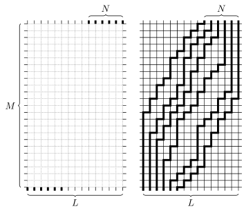
Figure 2. Boundary conditions of the model (left) and a possible configuration (right). Here $L=15$, $M=25$, and $N=6$.

The partition function of the model is defined as

$$Z_{L,M,N}(a,b,c)=\sum_{\text{conf}}a^{\#a}b^{\#b}c^{\#c}$$ (1.1)

where the sum is taken over all possible configurations of the model and $\#a$, $\#b$ and $\#c$ denote the number of vertices of type $a$, $b$ and $c$, respectively.

A specific feature of the four-vertex model with fixed boundary conditions is that the number of vertices of each type does not depend on the configuration. In particular, in our case we have

$$\#a=(L-N)(M-N),\quad\#b=N(M-L+N),\quad\#c=2N(L-N),$$ (1.2)

and thus

$$Z_{L,M,N}(a,b,c)=a^{(L-N)(M-N)}b^{N(M-L+N)}c^{2N(L-N)}Z_{L,M,N}$$ (1.3)

where $Z_{L,M,N}$ is the number of allowed configurations. Therefore, with no loss of generality, we set $a=b=c=1$. Correspondingly, the Gibbs measure is uniform on the space of configurations of the model, and equal to $1/Z_{L,M,N}$.

1.2. Statement of the problem

The four-vertex model may exhibit, under suitable choice of fixed boundary conditions, the limit shape phenomenon. In particular, in the case of the scalar-product boundary conditions, in the scaling limit one observes the emergence of a central disordered region and six frozen regions: four of ferroelectric order (only $a$-, or only $b$-vertices) and two of anti-ferroelectric order (only $c$-vertices, alternating and forming a zig-zag pattern), see Fig. 3.

Figure 3. A typical configuration of the model. The central disordered region and the six ordered ones, of type $a$, $b$, and $c$, are clearly visible. Here $N=30$, $L=70$, and $M=120$.

To further illustrate this phenomenon, we have performed the following numerical experiment. We have generated $10^{5}$ configurations of the model on the lattice with $N=60$, $L=140$, $M=240$. We have used the Markov Chain Monte Carlo method with Coupling From The Past [PW-96], to ensure uniform sampling. In Fig. 4 we show the density of vertices of type $a$, $b$, and $c$, respectively, averaged over $10^{5}$ configurations.

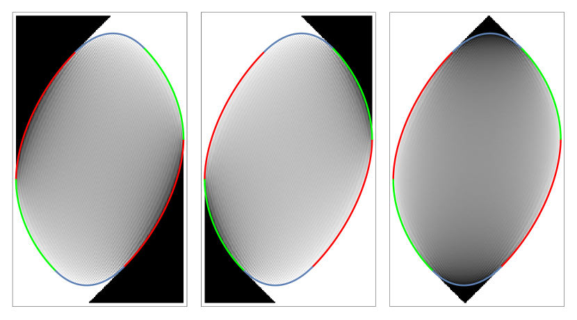
Figure 4. Densities of vertices of type $a$, $b$, and $c$ (left to right), with color varying from white to black as densities vary from 0 to 1. The picture has been generated by averaging over $10^{5}$ configurations of a lattice with $N=60$, $L=140$, $M=240$. The arctic curve, as given in Thm. 1, below, is also plotted.

The simulation clearly shows the emergence of the six frozen regions of type $a$, $b$, and $c$, in black in the first, second, and third picture, respectively. These are sharply separated from the central disordered region by a smoth curve, known as the arctic curve.

The purpose of the present paper is twofold: on the one hand, to provide an explicit analytic expression for the arctic curve of the model, and on the other hand, to test and improve available methods to make them more effective, and applicable to a broader range of situations. In particular, below, we extend the Tangent Method to make it applicable in situations where the arctic curve separates the disordered region from an anti-ferroelectically frozen one, such as in the top part of Fig. 4, right. Also, we test the still conjectural validity of the Tangent Method by providing an alternative, rigorous derivation of our results.

1.3. Main result

Our main result is an explicit expression for the arctic curve of the model. This emerges in the scaling limit, defined as follows. First the sizes of the considered domain $L$, $M$, and $N$, and the lattice coordinates $n$ and $m$, are rescaled by a parameter $\ell$,

$$L=\lceil\mathcal{L}\ell\rceil,\quad M=\lceil\mathcal{M}\ell\rceil,\quad N=\lceil\mathcal{N}\ell\rceil,\quad n=\lceil x\ell\rceil,\quad m=\lceil y\ell\rceil,$$ (1.4)

and next the limit $\ell\to\infty$ is taken. The coordinates $x$ and $y$ parametrize the rescaled domain, $(x,y)\in[0,\mathcal{L}]\times[0,\mathcal{M}]$.

It appears that the arctic curve is made of six consecutive arcs, joined end by end at six ‘contact points’, $P_{1},\dots,P_{6}$, see Fig. 5. Each arc is a specific portion of some algebraic curve (actually, of some ellipse). We denote these six arcs by $\Gamma_{j}$, $j=1,\dots,6$, starting from the west contact point, $P_{1}$, and in clockwise order. These arcs separate a central disordered region from six different frozen regions of type $a$, $c$, $b$, and again $a$, $c$, $b$, respectively.

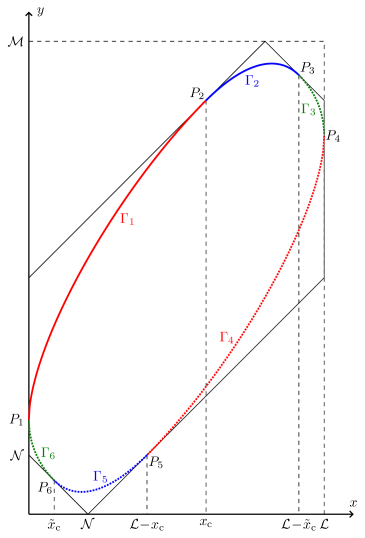
Figure 5. Arctic curve for the four-vertex model, with its six contact points. The solid portion is given by Thm. 1. The dotted portion may be restored from the symmetries of the model. Here $\mathcal{N:L:M}=1:5:8$.

Theorem 1.

The portions $\Gamma_{1}$ and $\Gamma_{2}$ of the arctic curve of the four-vertex model with the scalar-product boundary conditions are described by the following equations:

$$\left\{\begin{aligned} \Gamma_{1}:\quad&y=f_{1}(\mathcal{L},\mathcal{M},\mathcal{N};x),\quad&&x\in(0,x_{\mathrm{c}}],\\ \Gamma_{2}:\quad&y=f_{2}(\mathcal{L},\mathcal{M},\mathcal{N};x),\quad&&x\in[x_{\mathrm{c}},\mathcal{L}-\tilde{x}_{\mathrm{c}}],\end{aligned}\right.$$ (1.5)

where

$$f_{1}(\mathcal{L},\mathcal{M},\mathcal{N};x) =\frac{\mathcal{MN}(\mathcal{L}-2x)+(\mathcal{M+N})\mathcal{L}x}{\mathcal{L}^{2}}$$ (1.6)

$$\qquad\qquad+2\frac{\sqrt{\mathcal{MN(L-N)(M-L)}(\mathcal{L}-x)x}}{\mathcal{L}^{2}},$$ (1.7)

$$f_{2}(\mathcal{L},\mathcal{M},\mathcal{N};x) =(\mathcal{L-M-N}-x)+2f_{1}(\mathcal{L},\mathcal{M},\mathcal{N};x),$$ (1.8)

and

$$x_{\mathrm{c}}=\frac{(\mathcal{M}-\mathcal{L})(\mathcal{L}-\mathcal{N})}{\mathcal{M}-\mathcal{L}+\mathcal{N}},\qquad\tilde{x}_{\mathrm{c}}=\frac{(\mathcal{M}-\mathcal{L})\mathcal{N}}{\mathcal{M-N}}.$$ (1.9)

Remark.

Below, we provide two different derivations of this result. The first one is based on the Tangent Method [CS-16], and its validity is therefore conditioned to that of the main assumptions underlying the method, see Sect. 3 for details. The second derivation, based on the study of some suitable correlation function, is instead fully rigorous, see Sect. 4.

One can easily find the expression for the remaining portions of the curve with the help of symmetry arguments. In particular, $\Gamma_{3}$ may be obtained from $\Gamma_{1}$ by means of the so-called ‘particle-hole’ symmetry, which implies, in the scaling limit, the invariance of the model under the simultaneous replacement $\mathcal{N}\to\mathcal{L-N}$, $x\to\mathcal{L}-x$, see Sec. 2.1 for details. We have

$$\Gamma_{3}:\quad y=f_{1}(\mathcal{L},\mathcal{M},\mathcal{L-N};\mathcal{L}-x),\qquad x\in[\mathcal{L}-\tilde{x}_{\mathrm{c}},\mathcal{L}].$$ (1.10)

Note in particular that $\tilde{x}_{\mathrm{c}}$ in (1.9) is obtained from $x_{\mathrm{c}}$ by replacing $\mathcal{N}\to\mathcal{L-N}$. Also, the particle-hole symmetry, when applied to $\Gamma_{2}$, implies that

$$f_{2}(\mathcal{L},\mathcal{M},\mathcal{L-N};\mathcal{L}-x)=f_{2}(\mathcal{L},\mathcal{M},\mathcal{N};x),\qquad x\in[x_{\mathrm{c}},\mathcal{L}-\tilde{x}_{\mathrm{c}}],$$ (1.11)

as it may be easily verified. Concerning the remaining three portions of the arctic curve, $\Gamma_{4},\Gamma_{5},\Gamma_{6}$, these may be obtained from $\Gamma_{1},\Gamma_{2},\Gamma_{3}$, respectively, by means of the reflection symmetry, consisting in implementing simultaneously the two changes of variables, $x\to\mathcal{L}-x$ and $y\to\mathcal{M}-y$, see Sec. 2.1.

Remark.

It is easily seen that the arctic curve, although continuous everywhere, together with its first derivative, does not correspond to a single algebraic curve. Indeed it is only piecewise analytic, with discontinuities in the second derivative at the six contact points. The non-analiticity of the arctic curve reflects the fact that the four-vertex model is not a free-fermion model.

Concerning our main result, a few comments are in order. First, we note that there is a natural bijection between the four-vertex model with scalar-product boundary conditions and non-intersecting lattice paths, or lozenge tilings of a hexagon, see Sect. 2.3 for details. Despite this bijection, the four-vertex model is genuinely non free-fermionic, arising as a particular limit of the five-vertex model [B-08b, BuP-21]. Indeed the bijection is somewhat ‘non-local’, in the sense that different portions of the lattice are deformed in different ways when going back and forth between the four-vertex model and the non-intersecting lattice paths. Also, investigation of the limit shape of the four-vertex model appears beyond current capabilities of the variational approach (however, see [KP-22] for recent developments).

Second, in view of the above mentioned bijection, it is clear that one could have deduced the expressions of the six portions of the arctic curve from suitable transformations of those worked out in [CLP-99] for the lozenge tilings of a hexagon. It is nevertheless worth providing an independent derivation, in particular because the modified version of the Tangent Method proposed here may be extended to other more sophisticated models, such as, for instance, the five-vertex model, exhibiting phase separation with regions of anti-ferroelectric order [dGKW-21].

Third, our results provide one additional example of the effectiveness of the Tangent Method for evaluating the arctic curve of various models of statistical mechanics that have a description in terms of paths.

Fourth, the alternative derivation of our main theorem, based on the evaluation of the asymptotic behaviour of some ‘gap probability’ of the model, immediately implies, as a by-product, that the fluctuations of the arctic curve, away from the contact points, are governed by the Tracy-Widom distribution [TW-94a, TW-94b]. This follows directly from the Fredholm determinant representations provided for the gap probabilities, see (4.24) and (4.25) below, and constitutes one more example in support of the universality of Tracy-Widom distribution [D-06].

Finally, one could wonder about the fluctuations of configurations in the vicinity of the contact points. It would be interesting to verify whether these are actually described by the Gaussian Unitary Ensemble corner process, in analogy with lozenge tilings and the ice-model [OR-06, GP-15, G-14].

The paper is organized as follows. In Sec. 2 we discuss some useful properties of the model. In Sec. 3 we derive the expression for the arctic curve, Thm. 1, using the Tangent Method. In Sec. 4 we provide an alternative derivation of the theorem, using the EFP Method. Additional technical derivations are given in three Appendices.

2. Some properties of the model

2.1. Reflection and particle-hole symmetries

Let us consider some symmetries of the set of configurations of the four-vertex model with scalar-product boundary conditions. A first, elementary symmetry of the model, is that under simultaneous reflections with respect to the horizontal and vertical axes. In terms of the lattice coordinates, this transformation reads

$$(n,m)\mapsto(L-n,M-m),$$ (2.1)

see Fig. 6. The symmetry under this transformation implies relations for observables of the model and is clearly preserved in the scaling limit. In particular, concerning the arctic curve, this makes it possible to determine the portions $\Gamma_{4}$, $\Gamma_{5}$, and $\Gamma_{6}$ of the arctic curve from the portions $\Gamma_{1}$, $\Gamma_{2}$, and $\Gamma_{3}$, respectively.

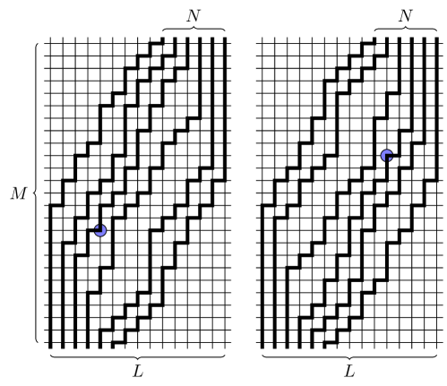
Figure 6. A configuration of the four-vertex model (left); the resulting configuration after simultaneous reflection with respect to both horizontal and vertical axes (right). The blue dot denotes the vertex of coordinates $(n,m)$ and its image under the transformation. Here $L=15$, $M=25$, $N=6$, $n=5$ and $m=10$.

Another symmetry is the following. If we swap the state (thick/thin) of each vertical edge and perform a reflection of the model with respect to an horizontal (or vertical) axis, we end up with a four-vertex model with the same type of boundary conditions, but with $L-N$ lines instead of $N$, see Fig. 7. This may be recognized as the usual particle-hole duality. The considered transformation corresponds to the following mapping of the lattice parameters and coordinates:

$$L,M,N\mapsto L,M,L-N,\qquad(n,m)\mapsto(L-n+1,m).$$ (2.2)

In particular, it follows that the northeast portion, $\Gamma_{3}$, of the arctic curve for the model with $N$ lines is readily obtained from the reflection of the northwest portion, $\Gamma_{1}$, of the arctic curve for the model with $L-N$ lines, see (1.10).

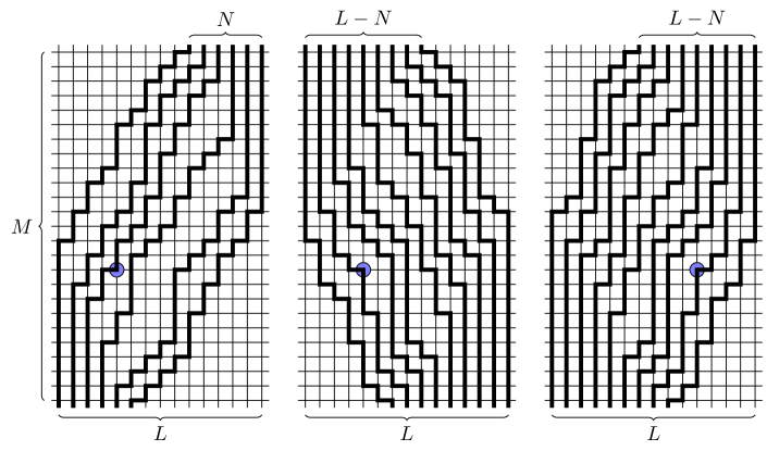
Figure 7. A configuration of the four-vertex model (left); the resulting configurations after swapping the state of all vertical edges (center), and next performing a reflection (right). The blue dot denotes the vertex $(n,m)$ and its image under the two transformations. Here $L=15$, $M=25$, $N=6$, $n=5$ and $m=10$.

2.2. Equivalent boundary conditions

It is easily seen that, due to the combinatorial constraints implied by the vertex rules (absence of the ‘all thick edges’ and of the ‘two horizontal thick edges’ vertex configurations), four triangular regions arise in the four corners, where all vertices are frozen. For instance, the vertices in the southwest triangular corner, with lattice coordinates $m+n\leq N$, are all of type $b$; similarly, the vertices in the northeast triangular corner, with lattice coordinates $m+n\geq M+L-N+2$, are again all of type $b$. In the same way, all vertices in the northwest triangular corner, $m-n\geq M-L+N+1$, and in the southeast one, $m-n\leq-N-1$, are of type $a$. Recalling that all Boltzmann weights are set to $1$, we may cut away these four triangular corners with no effect on the Boltzmann weights of the configurations, nor on the partition function. After that we are left with the model on a hexagonal domain, see Fig. 8.

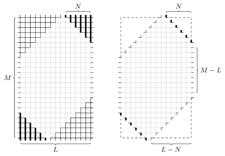
Figure 8. The four-vertex model on the rectangular domain, with the four frozen triangular regions (left), and on the hexagonal domain (right).

2.3. Four-vertex model and non-intersecting lattice paths

There exists a natural bijection between the configurations of the four-vertex model and non-intersecting lattice paths, corresponding to that between strictly decreasing and ordinary boxed plane partitions. In terms of paths, the bijection is based on two facts: first, each configuration is uniquely determined by the positions of the thick horizontal edges, and, second, each path has exactly $L-N$ such edges. If we shift the $i$-th horizontal thick edge ($i=1,\dots,L-N$, counting from the southwest) of each path by $i-1$ lattice spacings southward, then we get a configuration of $N$ non-intersecting lattice paths on the $L\times K$ lattice, $K=M-L+N+1$, with no further constraint, see Fig. 9. In this new setting, the $j$th path, $j=1,\dots,N$ connects the vertices of coordinates $(j,1)$ and $(L-N+j,K)$.

Figure 9. A configuration of the four-vertex model (left), and the corresponding configuration of non-intersecting lattice paths (right). Here $L=15$, $M=25$, $N=6$, and thus $K=17$.

Note that, in the non-intersecting lattice path version of the model, due to combinatorial constraints, we may replace the vertical paths in the southwest and northeast corners of the lattice with horizontal ones, or may even simply remove these corners alltogether, obtaining the same result. In other words, we could have equivalently considered, as southwest endpoints of the $j$th path, $j=1,\dots,N$, the vertices $(1,N-j+1)$, or the vertices $(j,N-j+1)$. Similarly, we could have considered as northeast endpoints the vertices $(L,K-j+1)$, or the vertices $(L-N+j,K-j+1)$, again obtaining the same result. This property will be sometimes used for simplicity, in the calculation of various correlation functions of the model, in the Appendices.

With the help of this bijection, by applying the Linström-Gessel-Viennot lemma [L-73, GV-85], see also [S-90], one can find explicit expressions for various quantities of interest of the model, the simplest being of course the partition function.

Proposition 2.

The partition function is given by

$$Z_{L,M,N}=\prod_{j=1}^{N}\frac{(j-1)!(M-N+j)!}{(L-N+j-1)!(M-L+j)!}.$$ (2.3)

The proof is very standard, see App. A for details.

Remark.

The above product may be equivalently rewritten as $\mathrm{PL}(N,L-N,M-L+1)$, where

$$\mathrm{PL}(r,s,t)=\prod_{i=1}^{r}\prod_{j=1}^{s}\prod_{k=1}^{t}\frac{i+j+k-1}{i+j+k-2}$$ (2.4)

is the famous Mac-Mahon formula for the number of plane partitions that fit in a box of size $r\times s\times t$.

The relation between boxed plane partitions and non-intersecting lattice paths is well known, see, e.g., [Br-99] and reference therein.

Remark.

It is clear from the last remark that, in order to have more that just one admissible configuration in the model, we must have $M\geq L>N$.

2.4. The boundary-refined partition function

A crucial role in the Tangent Method is played by the boundary-refined partition function, defined as follows. Let us consider a generic configuration of the system on the hexagonal domain and focus on the trajectory of the leftmost path. Starting from the southmost vertex $(1,1)$ such a path will consist of a sequence of $b$- and $c$-vertices. There is clearly a last vertex of type $b$. Denoting its horizontal coordinate by $n$, $n\in[1,L-N+1]$, its vertical coordinate is $m=n+M-L+N-1$, see Fig. 10.

We may thus define the boundary-refined partition function $Z_{L,M,N}^{(1)}(n)$, that enumerates the configurations of the model according to the horizontal coordinate of the last $b$ vertex of the leftmost path.

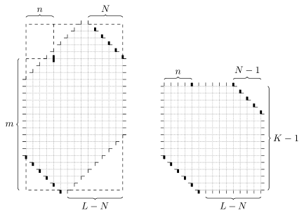
Figure 10. The boundary conditions defining the boundary-refined partition function $Z_{L,M,N}^{(1)}(n)$ of the four-vertex model (left), and the corresponding picture in terms of non-intersecting lattice paths (right). Here $L=15$, $M=25$, $N=6$, and $n=5$, implying $K=17$ and $m=20$.

Proposition 3.

The number of configurations conditioned to have a vertex of type $b$ at position $(n,n+M-L+N-1)$ is given by

$$Z_{L,M,N}^{(1)}(n)=\frac{(M-L-1+n)!(L-n)!}{(n-1)!(L-n-N+1)!(M-L+N-1)!}Z_{L,M-1,N-1}.$$ (2.5)

The proof, based on the above mentioned bijection with non-intersecting lattice paths, is given in App. A.

Remark.

It follows from the definition of the partition function and its boundary-refined counterpart that

$$\sum_{n=1}^{L-N+1}Z_{L,M,N}^{(1)}(n)=Z_{L,M,N},$$ (2.6)

as it may be verified by direct calculation.

Resorting to the bijection between the four-vertex model and non-intersecting lattice paths, one may also evaluate more sophisticated correlation functions. In this respect, a fundamental building block is what we name ‘column-refined partition function’, that is the partition function of the model, when conditioned to have all its thick edges in a given column at assigned positions, see App. B for a precise definition. Partial summations over the positions of these thick edges allows for the evaluation of various interesting correlation functions. We provide a derivation of the column-refined partition function for non-intersecting lattice paths in App. B. The obtained expression, evidenty related to discrete log-gases, is used in App. C to evaluate EFP and AFP in the four-vertex model.

3. Arctic curve via the Tangent Method

In this section we apply the Tangent Method [CS-16] to obtain the arctic curve of the model. The method is based on considering a slight modification of the boundary conditions, and hence of the configurations of the model. Since the required modification is different for various portions of the curve, we treat them separately.

3.1. Determination of the ferroelectric/disorder interface

To start with, we focus on the northwest portion $\Gamma_{1}$ of the arctic curve. To obtain its explicit expression, we slightly modify the boundary condition by moving the north extremal edge of the leftmost path from the $(L-N+1)$th vertical edge of the north boundary to the $r$th one, where $r\leq L-N$, see Fig. 11.

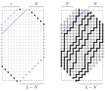
Figure 11. Modified boundary conditions, with $r=7$ (left), and a possible configuration, with $p=5$ (right). The blue line indicates the northwest boundary of the hexagonal domain.

The main assumption of the Tangent Method is that in the scaling limit such a path first follows the arctic curve, and then departs tangentially from it and becomes a straight line that intersects the north boundary of the domain at the point corresponding to (the rescaled value of) $r$. Note that despite its intuitiveness, such a behaviour is still conjectural in general. Rigorous results have been derived in some particular cases [A-20, DGR-19]. Later on we shall show that the conjectural arctic curve obtained through the Tangent Method, besides being well supported by numerical simulations, may also be derived rigorously by performing the asymptotic analysis of some suitable correlation functions.

Let us denote the partition function of the model with the modified boundary conditions by $\tilde{Z}_{L,M,N}^{(1)}(r)$. We can split the corresponding modified domain into two parts: the hexagonal domain and the northwest triangular region. For any given configuration on the modified domain, let us denote by $p$ the horizontal coordinate of the vertex where the leftmost path, arriving from southwest, first touches the border $m=n+M-L+N$. Note that this implies the presence of a $b$-vertex at position $(p,p+M-L+N-1)$, see Fig. 11. With this setting, the partition function may be expressed as

$$\tilde{Z}_{L,M,N}^{(1)}(r)=\sum_{p=1}^{r}Z_{L,M,N}^{(1)}(p)E_{L,M,N}^{(1)}(p,r),$$ (3.1)

where $Z_{L,M,N}^{(1)}(p)$ is the boundary-refined partition function defined in Sect. 2.4, and $E_{L,M,N}^{(1)}(p,r)$ is the partition function of the triangular extension, with a path connecting the vertices of coordinates $(p,p+M-L+N)$ and $(r,M)$, see Fig. 12.

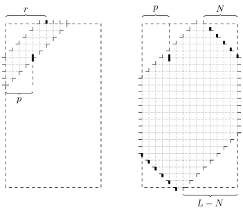
Figure 12. The boundary conditions on the triangular extension, corresponding to $E_{L,M,N}^{(1)}(p,r)$ (left) and on the hexagonal domain, corresponding to the boundary-refined partition functions $Z_{L,M,N}^{(1)}(p)$ (right).

The quantity $E_{L,M,N}^{(1)}(p,r)$ is easily evaluated, being simply the number of configurations for a single path from $(p,p+M-L+N)$ to $(r,M)$, satisfying the four-vertex rules, or equivalently, the number of configurations for a directed lattice path from $(p,M-L+N+1)$ to $(r,M-r+1)$. One has

$$E_{L,M,N}^{(1)}(p,r)=\binom{L-N-p}{r-p}.$$ (3.2)

As for $Z_{L,M,N}^{(1)}(p)$, we resort to Prop. 3.

We are interested in studying $\tilde{Z}_{L,M,N}^{(1)}(r)$ in the scaling limit. To this aim, we rescale the parameters as in (1.4), and also

$$p=\lceil t\ell\rceil,\qquad r=\lceil u\ell\rceil,$$ (3.3)

with $t\in(0,u]$ and $u\in(0,\mathcal{L}-\mathcal{N}]$, and send $\ell\to\infty$. Expression (3.1) may be interpreted as a Riemann sum. In the large $\ell$ limit, this becomes an integral, and can be evaluated by the saddle-point method. We are thus led to define the ‘action’

$$S^{(1)}(t,u):= \lim_{\ell\to\infty}\frac{1}{\ell}\log\left[\frac{Z_{L,M,N}^{(1)}(p)E_{L,M,N}^{(1)}(p,r)}{Z_{L,M,N}}\right]$$

$$= (\mathcal{L}-t)\log(\mathcal{L}-t)+(\mathcal{M}-\mathcal{L}+t)\log(\mathcal{M}-\mathcal{L}+t)$$

$$\qquad-(u-t)\log(u-t)-t\log t+\dots,$$ (3.4)

where, in the last line, we have dropped terms that do not depend on $t$. The saddle-point equation reads

$$0=\frac{\differential\ }{\differential t}S^{(1)}(t,u)=\log\frac{(\mathcal{M}-\mathcal{L}+t)(u-t)}{t(\mathcal{L}-t)}.$$ (3.5)

It is easily verified that its unique solution,

$$t_{0}=\frac{\mathcal{M}-\mathcal{L}}{\mathcal{M}-u}u,$$ (3.6)

corresponds to a maximum of $S^{(1)}(t,u)$. We have thus shown that, for any given value of $u\in(0,\mathcal{L}-\mathcal{N}]$, the leftmost path exits the hexagonal domain at some value $t$ that concentrates around $t_{0}$. We conclude that in the scaling limit the upper portion of such path follows the straight line through the points $(t_{0},\mathcal{M-L+N}+t_{0})$ and $(u,\mathcal{M})$.

Let us now proceed with the derivation of the curve. According to the Tangent Method the west arc is the envelope of the one-parametric family of lines passing through the two points specified above, that is,

$$(y-\mathcal{M})(t_{0}-u)=(x-u)(\mathcal{N}-\mathcal{L}+t_{0}),\qquad u\in(0,\mathcal{L-N}],$$ (3.7)

or, using (3.6) to eliminate $t_{0}$,

$$u(u-\mathcal{L})y+[\mathcal{M}(\mathcal{L}-\mathcal{N}-u)+\mathcal{N}u]x+\mathcal{N}(\mathcal{M}-u)u=0,\qquad u\in(0,\mathcal{L-N}].$$ (3.8)

The envelope is easily evaluated by differentiating with respect to $u$,

$$(\mathcal{L}-2u)y+(\mathcal{M}-\mathcal{N})x-\mathcal{N}(\mathcal{M}-2u)=0,$$ (3.9)

and solving the obtained pair of equations for $x$ and $y$, with the result

$$x(u)= \frac{\mathcal{N}(\mathcal{M-L})u^{2}}{(\mathcal{M-N})u^{2}-2\mathcal{M}(\mathcal{L-N})u+\mathcal{LM(L-N)}},$$ (3.10)

$$y(u)= \frac{\mathcal{N(M-N)}u^{2}-2\mathcal{MN(L-N)}u+\mathcal{M}^{2}\mathcal{N(L-N)}}{(\mathcal{M-N})u^{2}-2\mathcal{M}(\mathcal{L-N})u+\mathcal{LM(L-N)}}.$$ (3.11)

The arc of the curve described by this last expression, as $u$ varies over the interval $(0,\mathcal{L-N})$, is the northwest portion of the arctic curve, $\Gamma_{1}$. Indeed it is easily verified that $(x(0),y(0))$ lies on the line $x=0$, that is the west boundary of the hexagonal domain, and that $(x(\mathcal{L-N}),y(\mathcal{L-N}))$ lies on the line $y=x+\mathcal{M-L+N}$, that is the northwest boundary of the hexagonal domain. Finally, note that $x(u)|_{u=\mathcal{L-N}}=x_{\mathrm{c}}$, with $x_{\mathrm{c}}$ given by (1.9).

The portion $\Gamma_{1}$ of the arctic curve may also be written in implicit form, by using (3.9) to eliminate $u$ in (3.8). It is then given by the portion of the algebraic curve (actually, an ellipse)

$$\left(\mathcal{L}y-\mathcal{NM}+(\mathcal{M-N})x\right)^{2}+4\mathcal{M}(\mathcal{L}-\mathcal{N})x(\mathcal{N}-y)=0$$ (3.12)

lying in the region $x\in[0,x_{\mathrm{c}}]$, $y\in[y(0),y(x_{\mathrm{c}})]$, with $y(0)=\mathcal{M}\mathcal{N}/\mathcal{L}$.

Solving the equation (3.12) for $y$ we find that

$$y=\frac{\mathcal{MN}(\mathcal{L}-2x)+(\mathcal{M+N})\mathcal{L}x}{\mathcal{L}^{2}}\pm\frac{2\sqrt{\mathcal{MN(M-L)(L-N)}(\mathcal{L}-x)x}}{\mathcal{L}^{2}}.$$ (3.13)

Since we are interested in the northwest portion of the arctic curve, we must choose the plus sign. We have thus obtained the expression (1.7) stated in Thm. 1. Note that our calculation here allows to determine only that portion of the arctic curve with $x\in(0,x_{\mathrm{c}}]$, corresponding to values of the slope of the tangent path decreasing from $+\infty$ to $1$.

3.2. Determination of the anti-ferroelectric/disorder interface

We now turn to the determination of the north portion, $\Gamma_{2}$ of the arctic curve. Note, however, that the frozen region adjacent to $\Gamma_{2}$ is fully packed of $c$ vertices, that is of zigzag paths, and the Tangent Method may not be applied directly, but requires a slightly involved preparation.

First we extend the hexagonal domain by adding a triangular region to its northeast side, consisting in the vertices of coordinates $\{(n,m)$: $L-N<n\leq L$, $\absolutevalue{m-M-1}<n-L+N\}$, and impose all vertices on its east boundary to be of type $c$ (starting with a vertex of the last type listed in Fig. 1, and alternating between the two types of $c$-vertices, see Fig. 13). Such boundary condition constrains all vertices in the triangular extension to be of type $c$, with the $N$ paths from the hexagonal domain being continued through the triangular extension with a zig-zag pattern, till the east boundary of the extended domain. The extension being frozen by construction, the configurations in the hexagonal domain and the partition function are left unaltered.

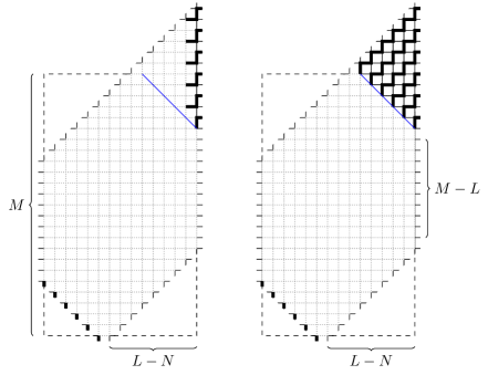
Figure 13. The hexagonal domain with the triangular extension, and the new boundary conditions (left); these induce freezing of the whole triangular region, while preserving the boundary conditions of the original hexagonal domain (right). The blue line indicates the nortwest boundary of the hexagonal domain.

Next we modify the boundary conditions on the east side by adding one vertex of type $a$ at position $(L,M+N-2r)$, $r=0,\dots,N$, and shifting the $2N-2r-1$ remaining vertices one position to the south, see Fig. 14. The meaning of this modification becomes clear when one focuses on the vertices of type $a$ and interprets them as particles. Then the configurations of the model are essentially configurations of two families of non-intersecting lattice paths, see Fig. 15. The topmost thin (blue) path is the relevant one for application of the Tangent Method in this extended context, see Fig. 15, right. For the sake of clarity, we have also extended the domain with two triangular regions of $a$ vertices.

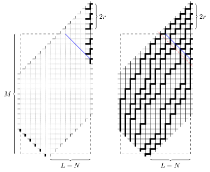
Figure 14. Modified boundary conditions, with $r=3$ (left), and a possible configuration (right). The blue line indicates the northwest boundary of the hexagonal domain. There is one and only one vertex of type $a$ lying on the dotted red line.

Figure 15. Configuration of the four-vertex model with original (left) and modified (right) boundary conditions in terms of two species of non-intersecting lattice paths. The topmost thin (blue) path in the right picture is the relevant one for the Tangent Method. Here $p=1$ and $r=3$. The dotted red line is as in Fig. 12.

Let us evaluate the quantity $\tilde{Z}_{L,M,N}^{(2)}(r)$, denoting the partition function of the model with the modified boundary conditions. Again, we may split the domain into two parts: the original hexagonal domain, and its triangular extension. For any given configuration on the extended domain with modified boundary conditions, there is one and only one vertex of type $a$ lying on the line $m+n=L-N+M$ (adjacent to the northeast boundary of the hexagonal domain, see Fig. 14, right). We may write the coordinates of such an $a$-vertex as $(L-N+p,M-p)$, and thus use $p=0,\dots,N$ to label its position. With this setting, the partition function of the model with modified boundary conditions may be expressed as

$$\tilde{Z}^{(2)}_{L,M,N}(r)=\sum_{p=0}^{r}Z^{(2)}_{L,M,N}(p)E^{(2)}_{L,M,N}(p,r),$$ (3.14)

where $Z^{(2)}_{L,M,N}(p)$ is the partition function on the hexagonal domain, conditioned to have a vertex of type $a$ at position $(L-N+p,M-p)$, and $E^{(2)}_{L,M,N}(p,r)$ is the partition function of the triangular extension. Referring to Fig. 15, right, focussing on the top blue path therein, and proceeding as for $E_{L,M,N}^{(1)}(p,r)$, see (3.2), it is easy to find that

$$E^{(2)}_{L,M,N}(p,r)=\binom{N-p}{r-p}.$$ (3.15)

As for the partition function $Z^{(2)}_{L,M,N}(p)$, using the particle-hole symmetry (2.2), we find that

$$Z^{(2)}_{L,M,N}(p)=Z_{L,M,L-N}^{(1)}(N-p+1),$$ (3.16)

where $Z_{L,M,N}^{(1)}(n)$ is the boundary-refined partition function, evaluated in (2.5).

We may now proceed to evaluate (3.14) in the scaling limit. Let us rescale the parameters and coordinates of the lattice variables as in (1.4). Let also $p=\lceil t\ell\rceil$ and $r=\lceil u\ell\rceil$, with $t\in[0,u]$ and $u\in[0,\mathcal{N}]$. Again, in the scaling limit, the sum in (3.14) turns into an integral whose values is dominated by the saddle-point of the ‘action’

$$S^{(2)}(t,u):= \lim_{\ell\to\infty}\frac{1}{\ell}\log\left[\frac{(M-L+N-p)!(L-N+p)!}{p!(N-p)!}\binom{N-p}{r-p}\right]$$ (3.17)

$$= (\mathcal{M-L+N}-t)\log(\mathcal{M-L+N}-t)+(\mathcal{L}-\mathcal{N}+t)\log(\mathcal{L}-\mathcal{N}+t)$$ (3.18)

$$\qquad-t\log t-(u-t)\log(u-t)-(\mathcal{N}-u)\log(\mathcal{N}-u),$$ (3.19)

namely

$$t_{0}=\frac{u(\mathcal{L}-\mathcal{N})}{\mathcal{M}-u}.$$ (3.20)

It is straigthforward to check that $t_{0}$ is the only stationary point of $S^{(2)}(t,u)$, that it actually corresponds to a maximum, and that it lies inside the interval $(0,u)$ for all values of $u\in(0,\mathcal{N})$.

Therefore in the scaling limit the diverted path becomes a straight line through $(\mathcal{L-N}+t_{0},\mathcal{M}-t_{0})$ and $(\mathcal{L},\mathcal{M+N}-2u)$. The arctic curve is the envelope of the family of such lines as $u\in[0,\mathcal{N}]$,

$$y=\frac{x-\mathcal{L}}{t_{0}-\mathcal{N}}(\mathcal{M}-t_{0})+\frac{x-(\mathcal{L}-\mathcal{N}+t_{0})}{\mathcal{N}-t_{0}}(\mathcal{M}+\mathcal{N}-2u),$$ (3.21)

or, substituting (3.20) for $t_{0}$,

$$\mathcal{MN}(\mathcal{M-L+N}-y+x-2u)+\mathcal{L}u(\mathcal{M-L+N}+x+y)\\ +2ux(u-\mathcal{M-N})=0.$$ (3.22)

Along the line of previous Section, differentiating the above expression with respect to $u$, and solving for $u$, we get

$$u=\frac{\mathcal{L}^{2}+2\mathcal{N}x+2\mathcal{M}(\mathcal{N}+x)-\mathcal{L}(\mathcal{M}+\mathcal{N}+x+y)}{4x}.$$ (3.23)

Substituting this in (3.22) and solving for $y$, we get

$$y=\mathcal{L-M-N}-x+2\,\frac{\mathcal{NM}(\mathcal{L}-2x)+(\mathcal{M+N})\mathcal{L}x}{\mathcal{L}^{2}}\\ \pm 4\,\frac{\sqrt{\mathcal{MN(M-L)(L-N)}(\mathcal{L}-x)x}}{\mathcal{L}^{2}}.$$ (3.24)

This curve is again an ellipse, although a different one, with respect to (3.12). Since we are interested in the north portion of the curve, we must choose the plus sign, thus obtaining the expression (1.8) stated in Thm. 1.

4. Arctic curve via the EFP Method

In this section we introduce two observables which we call ‘Emptiness Formation Probability’ (EFP) and ‘Anti-ferroelectric phase Formation Probability’ (AFP). We express these functions in terms of gap probabilities for discrete log-gases associated to the measure of Hahn polynomials. Then, following [J-02], and using the results of [BKMM-07] for the asymptotic behaviour of these quantities in the scaling limit, we derive an expression for the arctic curve, and determine its fluctuations.

4.1. EFP and AFP

Let us consider, in the rectangular domain, the topmost $q$ consecutive vertices in the $p$th vertical line, $p\leq L-N$, that is the vertices of coordinates $(p,M-j+1)$, $j=1,\dots,q$. Let $\Theta$ be the subset of such vertices contained in the hexagonal domain, that is the vertices of coordinates $(p,M-q+j)$, $j=1,\dots,\tilde{q}$, with $\tilde{q}:=p+q-L+N$. Let $\Omega$ be the set of all configurations of the model, and $\Omega^{\mathrm{I}}_{p,q}$, $\Omega^{\mathrm{II}}_{p,q}$ the sets of configurations in which all vertices in $\Theta$ are of type $a$, or $c$, respectively. We may now introduce two observables, the EFP and the AFP, denoted as $F_{L,M,N}(p,q)$ and $G_{L,M,N}(p,q)$, respectively, and defined as

$$F_{L,M,N}(p,q):=\frac{\absolutevalue{\Omega^{\mathrm{I}}_{p,q}}}{\absolutevalue{\Omega}},\qquad G_{L,M,N}(p,q):=\frac{\absolutevalue{\Omega^{\mathrm{II}}_{p,q}}}{\absolutevalue{\Omega}},$$ (4.1)

where $\absolutevalue{\Omega}$ stands for the cardinality of $\Omega$.

Note, that, in view of the chosen boundary conditions, the request of having all vertices in $\Theta$ of type $a$ (for EFP) or $c$ (for AFP) implies the existence of a subregion in the hexagonal lattice where all vertices are of type $a$, or $c$, respectively, see Fig. 16.

In what follows we will always assume that

$$p+q>L-N,$$ (4.2)

which guarantees that $\Theta$ is non empty, and also

$$p\leq L-N,\qquad p+q<M-N,$$ (4.3)

for EFP, and

$$p+q>L-N,\qquad p\leq L-N,\qquad p+q\leq M-N$$ (4.4)

for AFP, guaranteeing that $\Omega^{\mathrm{I}}_{p,q}$ and $\Omega^{\mathrm{II}}_{p,q}$, respectively, are non empty; if this were the case, the corresponding formation probabilities would simply vanish.

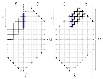
Figure 16. Subregions of the hexagonal domain that are frozen, due to the condition imposed on the vertices in $\Theta$ (shaded), in the case of EFP (left) and AFP (right). Here $L=15$, $M=25$, $N=6$, $p=7$, $q=8$, and $\tilde{q}=6$.

4.2. Log-gas representations

We now turn to the evaluation of some representations of EFP and AFP in terms of discrete log-gases [F-10]. To start with, let us introduce the Hahn measure,

$$w^{(\alpha,\beta)}_{n}(x)=\binom{\alpha+x}{x}\binom{\beta+n-x}{n-x},$$ (4.5)

defined on the discrete interval $x\in[0,n]$. When the parameters $\alpha,\beta>-1$ or $\alpha,\beta<-n$, we may define the corresponding family of orthogonal polynomials $\{Q^{(\alpha,\beta)}_{k,n}(x)\}_{k=0,\dots,n}$, satisfying the orthonormality condition

$$\sum_{x=0}^{n}w^{(\alpha,\beta)}_{n}(x)Q^{(\alpha,\beta)}_{k,n}(x)Q^{(\alpha,\beta)}_{l,n}(x)=\delta_{k,l}.$$ (4.6)

The polynomials

$$Q^{(\alpha,\beta)}_{k,n}(x)=(-1)^{k}\sqrt{\binom{n}{k}\frac{n!(2k+\alpha+\beta+1)(\alpha+1)_{k}(\alpha+\beta+1)_{k}}{(\alpha+\beta+1)_{n+1}(\beta+1)_{k}(n+\alpha+\beta+2)_{k}}}\\ \times\,{}_{3}F_{2}\left(\left.\genfrac{}{}{0.0pt}{}{-k,\,k+\alpha+\beta+1,\,-x}{\alpha+1,\,-n}\right|1\right),\qquad k=0,\dots,n,$$ (4.7)

are known as (normalized) Hahn polynomials [KLS-10].

We are now ready to introduce the Hahn log-gas. Let $\mathbf{x}:=\{x_{1},\dots,x_{s}\}$, with $0\leq x_{1}<\dots<x_{s}\leq n$, denote the ordered set of positions of $s$ particles on the discrete interval $[0,n]$. Consider the probability measure on $[0,n]^{s}$, defined as

$$P^{(\alpha,\beta)}_{n,s}[\mathbf{x}]=\frac{1}{Z(\alpha,\beta,s,n)}\prod_{1\leq i<j\leq s}(x_{i}-x_{j})^{2}\prod_{j=1}^{s}w^{(\alpha,\beta)}_{n}(x_{j})$$ (4.8)

where $w^{(\alpha,\beta)}_{n}(x)$ is the Hahn measure (4.5). The normalization constant

$$Z(\alpha,\beta,s,n)=\sum_{0\leq\mathbf{x}\leq n}\prod_{1\leq i<j\leq s}(x_{i}-x_{j})^{2}\prod_{j=1}^{s}w_{n}^{(\alpha,\beta)}(x_{j})$$ (4.9)

is the partition function of the log-gas.

Remark.

The partition function $Z(\alpha,\beta,s,n)$ may also be represented as the determinant of a Hankel matrix,

$$Z(\alpha,\beta,s,n)=\det_{1\leq i,j\leq s}\left[\sum_{x=0}^{n}x^{i+j-2}w_{n}^{(\alpha,\beta)}(x)\right],$$ (4.10)

whose elements are the moments of Hahn measure. In principle, this could allow for a direct evaluation of the partition functions in terms of the leading coefficients of orthonormal Hahn polynomials.

Let us introduce also the function

$$H(d,\alpha,\beta,s,n):=\sum_{0\leq\mathbf{x}\leq d}P^{(\alpha,\beta)}_{n,s}[\mathbf{x}],$$ (4.11)

with $d\leq n$, which is nothing but the ‘gap probability’, that is, the probability of having, in the Hahn log-gas of $s$ particles, no particle with coordinate larger that $d$. Clearly, the gap probability may be rewritten as a Hankel determinant, just as done above for the partition function, see (4.10).

We may now state three propositions expressing EFP and AFP in terms of discrete Hahn log-gases. The proof of these propositions, based on the bijection from the four-vertex model to non-intersecting lattice paths, is provided in App. C.

Proposition 4.

EFP $F_{L,M,N}(p,q)$ is given by

$$F_{L,M,N}(p,q)=H(d,\alpha,\beta,s,n)$$ (4.12)

with parameters

$$d=M-N+\min(p,N)-p-q,\qquad\alpha=\absolutevalue{N-p},\qquad\beta=L-N-p,$$ (4.13)

$$s=\min(p,N),\qquad n=M-L+\min(p,N).$$ (4.14)

Remark.

The conditions $\alpha>-1$ and $\beta>-1$, entering the definition of the orthogonalizing measure for Hahn polynomials, are always fulfilled here. This is evident for $\alpha$; as for $\beta$, recall that when $p>L-N$, $F_{L,M,N}(p,q)=0$ by construction, see (4.3).

Proposition 5.

AFP is related to EFP as follows:

$$G_{L,M,N}(p,q)=F_{M-L+N+1,M,M-L+1}\left(\tilde{r},L-\tilde{p}\right),$$ (4.15)

where $\tilde{r}=\big{\lfloor}\frac{\tilde{q}+1}{2}\big{\rfloor}$, $\tilde{p}=p-\mathrm{mod}(\tilde{q}+1,2)$, and $\tilde{q}=p+q-L+N$.

In turn, these imply the following explicit representation for AFP.

Proposition 6.

AFP $G_{L,M,N}(p,q)$ is given by

$$G_{L,M,N}(p,q)=H(d,\alpha,\beta,s,n)$$ (4.16)

with parameters

$$d=L-N+\min(\tilde{r},M-L+1)-2-q+\tilde{r},$$ (4.17)

$$\alpha=\absolutevalue{M-L-\tilde{r}+1},\qquad\beta=N-\tilde{r},$$ (4.18)

$$s=\min(\tilde{r},M-L+1),\qquad n=L-N+\min(\tilde{r},M-L+1)-1,$$ (4.19)

where $\tilde{r}=\big{\lfloor}\frac{\tilde{q}+1}{2}\big{\rfloor}=\big{\lfloor}\frac{p+q-L+N+1}{2}\big{\rfloor}$.

Remark.

The conditions $\alpha>-1$ and $\beta>-1$, entering the definition of the orthogonalizing measure for Hahn polynomials, are always fulfilled here as well. Again, this is evident for $\alpha$; as for $\beta$, recall that when $\tilde{r}>N$, $G_{L,M,N}(p,q)=0$ by construction, see (4.4).

4.3. Arctic curve

To find the arctic curve we need to study the asymptotic behaviour of EFP and AFP, or equivalently of the function $H(d,\alpha,\beta,s,n)$, when $d,\alpha,\beta,s,n\to\infty$ with fixed ratios. In such a limit, $H(d,\alpha,\beta,s,n)$ is known to tend to one if the values of the parameters are such that the vertices in $\Theta$ are all in a frozen region, and to zero otherwise. The arctic curve is characterized by separating these two regimes, see, e.g., [J-00, J-02].

In order to analize the asymptotic behaviour of $H(d,\alpha,\beta,s,n)$ in the desired scaling limit, one may resort to various technologies inspired from and related to random matrix models and the theory of orthogonal polynomials.

To start with, we set

$$d=\lfloor d_{0}\ell\rfloor,\qquad\alpha=\lfloor\alpha_{0}\ell\rfloor,\qquad\beta=\lfloor\beta_{0}\ell\rfloor,\qquad s=\lceil s_{0}\ell\rceil,\qquad n=\lceil n_{0}\ell\rceil,$$ (4.20)

with $\alpha_{0},\beta_{0}>0$ and $s_{0}<d_{0}<n_{0}$. Following standard methods from the theory of random matrix models, we rescale the coordinates, $x_{j}=\lfloor\mu_{j}\ell\rfloor$, $j=1,\dots,s$. The sums over $x_{j}$’s may be interpreted as Riemann sums, and, in the large $\ell$ limit, replaced by integrals. Correspondingly, we introduce the density $\rho(\mu)$, such that

$$\int_{0}^{n_{0}}\rho(\mu)\differential\mu=s_{0},\qquad 0\leq\rho(\mu)\leq 1.$$ (4.21)

The first equation is the usual normalization condition, while the second one is an additional constraint following from the discreteness of the original variables $x_{j}$ [DK-93].

In general, the density function $\rho(\mu)$ may be computed either by directly solving a suitable variational problem [BKMM-07] or by resorting to an integral representation based on the asymptotics of the recursion coefficients for the associated orthogonal polynomials [KA-99]. When the primary interest lies in determining the sole support of the density, rather than obtaining its complete expression, the latter approach proves to be much more efficient, see e.g. [J-02]. This is precisely the case when determining the arctic curve. Indeed, denoting by $R(\alpha_{0},\beta_{0},s_{0},n_{0})$ the right endpoint of the support of the density, the arctic curve is determined by the condition

$$R(\alpha_{0},\beta_{0},s_{0},n_{0})=d_{0},$$ (4.22)

see, e.g., [J-00].

Hahn polynomials have been extensively studied in the literature, therefore to get the expression of the corresponding density function we resort to [BKMM-07]. Specifically, for the right endpoint of the support of the density, see Eq. (276) therein. In our notations, it reads:

$$R(\alpha_{0},\beta_{0},s_{0},n_{0})=\\ =\left(\frac{\sqrt{(s_{0}+\alpha_{0}+\beta_{0})(s_{0}+\alpha_{0})(n_{0}-s_{0})}+\sqrt{(s_{0}+\alpha_{0}+\beta_{0}+n_{0})(s_{0}+\beta_{0})s_{0}}}{(2s_{0}+\alpha_{0}+\beta_{0})}\right)^{2}.$$ (4.23)

Inserting now (4.23) into (4.22), and specializing the parameters $\alpha_{0}$, $\beta_{0}$, $s_{0}$, $n_{0}$, $d_{0}$ according to Prop. 4, we recover expression (1.7) for the portion $\Gamma_{1}$ of the arctic curve. In a similar way, specializing the parameters $\alpha_{0}$, $\beta_{0}$, $s_{0}$, $n_{0}$, $d_{0}$ according to Prop. 6, we recover expression (1.8) for the portion $\Gamma_{2}$ of the arctic curve.

4.4. Arctic curve fluctuations

Having derived the arctic curve of the four-vertex model, the natural question to address next is that of its fluctuations. In view of the close relation of the model with non-intersecting lattice paths, or with lozenge tilings of a hexagon, we expect these fluctuations to be again governed by Tracy–Widom distribution [TW-94a, TW-94b]. Indeed, having expressed EFP and AFP as gap probabilities for the discrete log-gas with the Hahn measure, the answer to this question follows from the results of [BKMM-07], see also [J-00, J-02].

To start with, we recall a very standard fact, namely that the ‘gap probability’ $H(d,\alpha,\beta,s,n)$ may be rewritten as a Fredholm determinant:

$$H(d,\alpha,\beta,s,n)=\det\left[1-K_{n,s}|_{(d,n]}\right],$$ (4.24)

where $K_{n,s}|_{(d,n]}$ is a discrete integral operator acting on $L^{2}(d,n]$ with kernel

$$K_{n,s}(x,y)=\sum_{k=0}^{s}Q_{k,n}^{(\alpha,\beta)}(x)Q_{k,n}^{(\alpha,\beta)}(y)\sqrt{w_{n}^{(\alpha,\beta)}(x)w_{n}^{(\alpha,\beta)}(y)},\qquad x,y\in[0,n],$$ (4.25)

that is the Christoffel–Darboux kernel for the Hahn polynomials (4.7).

Let us now focus on the fluctuations of the portion $\Gamma_{1}$ of the Arctic curve. Our starting point is the expression for EFP, as given in Prop. 4. Let us consider values of $p$ within the interval $[N,p_{\mathrm{max}}]$, for some $p_{\mathrm{max}}<\lfloor(M-L)(L-N)/(M-L+N)\rfloor$. The lower bound has been chosen for simplicity, while the upper bound is such that, when setting $p=\lfloor x\ell\rfloor$, in the scaling limit one has $x\leq x_{\mathrm{max}}<x_{\mathrm{c}}$, see (1.9), and the considered portion of $\Gamma_{1}$ is thus away from the contact point. The expression for EFP simplifies to

$$F_{L,M,N}(p,q)=H(M-p-q,p-N,L-N-p,N,M-L+N),$$ (4.26)

with $p\in[N,p_{\mathrm{max}}]$. Let us fix a value of $p$, and denote by $\xi$ the value of the topmost thick edge between the $p$th and $(p+1)$th vertical lines of the $L\times M$ lattice. It follows from the definition of EFP that

$$\mathbb{P}(\xi<M-q)=F_{L,M,N}(p,q).$$ (4.27)

Recalling now (4.24) and (4.26), we may write

$$\mathbb{P}(\xi<M-q)=\det[1-K_{M-L+N,N}|_{(M-p-q,M-L+N]}],$$ (4.28)

with parameters $\alpha$ and $\beta$ of the Hahn measure specialized to $\alpha=p-N$ and $\beta=L-N-p$.

We may now consider values of $M-q$ in the vicinity of the portion $\Gamma_{1}$ of the arctic curve, as given by Thm. 1. In the non-intersecting lattice path picture, see Sect. 2.3, this amounts to consider values $M-q$ in the vicinity of $p+\ell R_{0}$, with $R_{0}:=R(\alpha_{0},\beta_{0},s_{0},n_{0})$ given by (4.23). It has been conjectured in [J-00], and proven in [BKMM-07], see Thm. 3.14 therein, that, in such regime, the Christoffel–Darboux kernel for the Hahn measure tends to the Airy kernel, in the scaling limit. Specifically, we have, for some constant $t>0$,

$$\lim_{\ell\to\infty}\mathbb{P}\left(\frac{\xi-p-\ell R(\alpha_{0},\beta_{0},s_{0},n_{0})}{(t\ell)^{1/3}}\leq x\right)=\det[1-A|_{(x,\infty)}],$$ (4.29)

where the integral operator $A|_{(x,\infty)}$ acts on $L^{2}[x,\infty)$ with the Airy kernel. In other words, the fluctuations of the considered portion of $\Gamma_{1}$ are indeed governed by the Tracy-Widom distribution.

One may proceed similarly for the fluctuations of the portion $\Gamma_{2}$ of the Arctic curve. However, on the one hand, the expression for AFP is more intricate, and, on the other hand, before applying the procedure carried out above for EFP, one should use particle-hole duality (in the sense of discrete log-gases on finite intervals, see Sect. 3.2 in [BKMM-07]). This makes the discussion slightly more involved, but leads to the conclusion that fluctuations of the portion $\Gamma_{2}$ of the Arctic curve, away from the contact points, are again governed by the Tracy–Widom distribution.

To conclude, we comment that Airy type density fluctuations in the vicinity of $\Gamma_{1}$ and $\Gamma_{4}$ are indeed clearly visible in Fig. 4, left, and similarly, for $\Gamma_{3}$ and $\Gamma_{6}$, in Fig. 4, center. However the phenomenon is not as apparent for $\Gamma_{2}$ nor $\Gamma_{6}$, in Fig. 4, right. This is due to the fact that oscillations in the densities of $c$-vertices of type 3 or 4, see Fig. 1, are in antiphase, and cancel out when considering the total density of $c$ vertices. To counter this problem, following [KL-17], we plot the difference between the two densities associated to the two types of $c$-vertices, see Fig. 17. Now Airy type density fluctuations in the vicinity of $\Gamma_{2}$ and $\Gamma_{5}$ become indeed clearly visible.

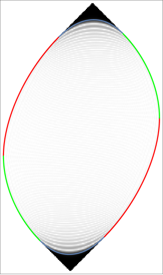
Figure 17. Absolute value of the difference of densities of $c$-vertices (that is of vertices of the third and fourth type, in Fig. 1), with color varying from white to black as densities vary from 0 to 1. The picture has been generated by averaging over $10^{5}$ configurations of the lattice with $N=60$, $L=140$, $M=240$.

Acknowledgments

We are indebted to N.M. Bogoliubov, L. Cantini, I. Prause, D. Serban, A. Sportiello, J.-M. Stéphan, J. Viti, for stimulating discussions at various stages of this work. FC and AM are grateful to the Workshop on ‘Randomness, Integrability, and Universality’, held on Spring 2022 at the Galileo Galilei Institute for Theoretical Physics, for hospitality and support at some stage of this work. AGP is grateful to INFN, Sezione di Firenze, for hospitality and partial support during his stay in Florence, Italy, where a part of this work was done. FC acknowledges partial support from Italian Ministry of Education, University and Research under the grant PRIN 2017E44HRF on ‘Low-dimensional quantum systems: theory, experiments and simulations’. AGP acknowledges support from the Russian Science Foundation, grant 21-11-00141.

Appendix A Boundary-refined partition function

We want here to evaluate the boundary-refined partition function. We shall resort to the bijection between configurations of the four-vertex model and non-intersecting lattice paths introduced in Sec. 2.3.

As a warm-up up, let us evaluate first the partition function $Z_{L,M,N}$. This is the number of configurations of $N$ lattice paths constrained by the four-vertex rules, with the the $j$th path, $j=1,\dots,N$, counting from the left, connecting the two vertices of coordinates $(j,1)$ and $(L-N+j,M)$, respectively, see Fig. 9, left. Such configurations are equinumerous with those of $N$ non-intersecting lattice paths connecting the vertices $(j,1)$ and $(L-N+j,K)$, with $K=M-L+N+1$, see Fig. 9, right. Using the Linström-Gessel-Viennot lemma [L-73, GV-85], we thus have:

$$Z_{L,M,N}=\det_{1\leq i,j\leq N}\left[\binom{M+i-j}{L-N+i-j}\right].$$ (A.1)

Determinants of matrices of binomials as above may be evaluated explicitly, see [K-01], Thm. 26, yielding (2.3).

Let us turn now to the boundary-refined partition function $Z_{L,M,N}^{(1)}(n)$. Recall that in the four-vertex model description, on the original rectangular lattice, we require the presence of a vertex of type $b$ at position $(n,m)$, with $m=n+M-L+N-1$, see Fig. 10, left. This means that the leftmost path, starting from vertex $(1,N)$, is constrained to reach the vertex $(n,m-1)$. As for the remaining paths, the $j$th one, $j=2,\dots,N$, must connect the vertices of coordinates $(j,N-j+1)$ and $(L-N+j,M-1)$.

In terms of non-intersecting lattice paths, the above conditions translate as follows: the $j$th path must connect the vertices of coordinates $(j,N-j+1)$ and $(x_{j},K-1)$, where $K=M-L+N+1$, and

$$x_{j}=\begin{cases}n,&\quad j=1,\\ L-N+j,&\quad j=2,\dots,N,\end{cases}$$ (A.2)

see Fig. 10, right. Application of Linström-Gessel-Viennot lemma directly yields

$$Z_{L,M,N}^{(1)}(n)=\det_{1\leq i,j\leq N}\binom{K-N-2+x_{j}}{x_{j}-i}.$$ (A.3)

The determinant of binomials in (A.3) can be evaluated explicitly:

$$Z_{L,M,N}^{(1)}(n)=\prod_{1\leq i<j\leq N}(x_{j}-x_{i})\prod_{j=1}^{N}\frac{(K-2+x_{j}-N)!}{(x_{j}-1)!(K-1-j)!}.$$ (A.4)

Taking into account (A.2), we find that

$$Z_{L,M,N}^{(1)}(n)=\frac{(M-L-1+n)!(L-n)!}{(n-1)!(L-N-n+1)!}\\ \times\frac{1}{(M-L+N-1)!}\prod_{2\leq i<j\leq N}(j-i)\prod_{j=2}^{N}\frac{(M-N-1+j)!}{(L-N+j-1)!(M-L+N-j)!}.$$ (A.5)

Simplifying further we easily recover (2.5).

Appendix B Column-refined partition function

Let us introduce here a quantity that, although somewhat intermediate, and formulated for the model of non-intersecting lattice paths, appears useful to evaluate the probability of occurrence of a variety of configurations in the four-vertex model.

Let us consider $N$ non-intersecting lattice paths on the $L\times K$ lattice, with our usual boundary conditions. In the spirit of [CDP-21], consider the partition function of the model when the paths are conditioned to flow through the $N$ horizontal edges lying in the $n$th column (i.e., between the $n$th and $(n+1)$th vertical lines), with ordinates $\mathbf{y}=\{y_{1},\dots,y_{N}\}$, such that $1\leq y_{1}<\dots<y_{N}\leq K$. We denote such partition function by $Z_{L,M,N}(n,\mathbf{y})$.

Note that we have reversed the labelling of paths, with respect to App. A. Also, it is convenient to use the freedom discussed in Sec. 2.3 to slightly change the boundary condition in such a way to have exactly $N$ horizontal thick edges in each column, including the first $N$ ones, and the last $N$ ones. We therefore choose as endpoints of the $j$th path, $j=1,\dots,N$, counting from the right, the vertices of coordinates $(1,j)$ and $(L,K-N+j)$, respectively, see Fig. 18.

Proposition 7.

The number of configurations of $N$ non-intersecting lattice paths, on the $L\times K$ lattice, with endpoints as mentioned above, and conditioned to flow through the horizontal edges at positions $(n,y_{1})$, …, $(n,y_{N})$, is:

$$Z_{L,M,N}(n,\mathbf{y})=C_{L,M,N;n}\prod_{j=1}^{\tilde{n}}\delta_{y_{j},j}\prod_{j=\tilde{l}+1}^{N}\delta_{y_{j},K-N+j}\prod_{\tilde{n}<i<j\leq\tilde{l}}(y_{j}-y_{i})^{2}\prod_{j=\tilde{n}+1}^{\tilde{l}}\mu(y_{j}),$$ (B.1)

where

$$\mu(y)=\binom{y-N+n+\tilde{n}-1}{y-\tilde{n}-1}\binom{K+L-n-\tilde{l}-y}{K-N+\tilde{l}-y}$$ (B.2)

and

$$C_{L,M,N;n}=\prod_{i=1}^{\tilde{n}}\frac{(i-1)!(K+L-N-n-i)!}{(K-N+\tilde{l}-i)!(L-n-i)!}\\ \times\prod_{i=\tilde{n}+1}^{\tilde{l}}\frac{(2\tilde{n}-N+n)!(L+N-n-2\tilde{l})!}{(i-N+n-1)!(L-n-i)!}\\ \times\prod_{i=\tilde{l}+1}^{N}\frac{(N-i)!(K-2N+n+i-1)!}{(K-N+\tilde{n}+i-1)!(i-N+n-1)!},$$ (B.3)

with $\tilde{n}=\max(N-n,0)$, and $\tilde{l}=\min(L-n,N)$.

Proof.

In order to evaluate $Z_{L,M,N}(n,\mathbf{y})$, let us split the lattice into two parts, by ‘cutting’ all horizontal edges between the $n$th and $(n+1)$th lines. It is natural to introduce two ‘wave functions’ $\Psi_{1}(\mathbf{y})$ and $\Psi_{2}(\mathbf{y})$, that, for a given configuration of thick horizontal edges, are the partition functions of the west and east portions of the split lattice, respectively, see Fig. 18.

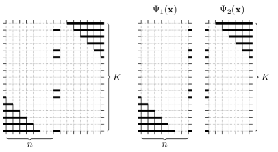
Figure 18. The column-refined partition function $Z_{L,M,N}(n,\mathbf{y})$ (left), and the two wave functions, $\psi_{1}(\mathbf{y})$ and $\psi_{2}(\mathbf{y})$ (right). Here $L=15$, $K=17$, $N=6$, $n=8$, and $\mathbf{y}=(1,6,7,12,13,16)$.

The two wave functions are easily calculated. Indeed $\Psi_{1}(\mathbf{y})$ is the number of configurations of $N$ non-intersecting lattice paths connecting the vertices of coordinates $(1,j)$ and $(n,y_{j})$, $j=1,\dots,N$. Similarly for $\Psi_{2}(\mathbf{y})$, but now with the vertices of coordinates $(n+1,y_{j})$ and $(L,K-N+j)$, $j=1,\dots,N$. Application of the Lindström-Gessel-Viennot lemma yields

$$\Psi_{1}(\mathbf{y}) =\det_{1\leq i,j\leq N}\left[\binom{y_{i}-j+n-1}{y_{i}-j}\right],$$ (B.4)

$$\Psi_{2}(\mathbf{y}) =\det_{1\leq i,j\leq N}\left[\binom{K-N+L-n-y_{i}+j-1}{K-N-y_{i}+j}\right].$$ (B.5)

These determinants evaluate to:

$$\Psi_{1}(\mathbf{y}) =\prod_{1\leq i<j\leq N}(y_{j}-y_{i})\prod_{i=1}^{N}\frac{(y_{i}-N+n-1)!}{(y_{i}-1)!(i-N+n-1)!},$$ (B.6)

$$\Psi_{2}(\mathbf{y}) =\prod_{1\leq i<j\leq N}(y_{j}-y_{i})\prod_{i=1}^{N}\frac{(K+L-N-n-y_{i})!}{(K-y_{i})!(L-n-i)!},$$ (B.7)

where, once more, we have used [K-01], Thm. 26.

Note that, strictly speaking, the expression (B.6) for $\Psi_{1}(\mathbf{y})$ is well defined only when $n\geq N$, being otherwise plagued with negative factorials. This corresponds to the fact that, when $n<N$, the $N-n$ lowest thick edges are constrained to $y_{j}=j$, $j=1,\dots,N-n$. Implementing such constraint, the negative factorials indeed cancel out, as it may be easily seen, e.g., interpreting them in terms of some suitable limit of corresponding Gamma functions. We obtain

$$\Psi_{1}(\mathbf{y})=\prod_{i=1}^{\tilde{n}}\delta_{y_{i},i}\prod_{\tilde{n}+1\leq i<j\leq N}(y_{j}-y_{i})\prod_{i=\tilde{n}+1}^{N}\frac{(y_{i}-N+n-1)!}{(y_{i}-\tilde{n}-1)!(i-N+n-1)!},$$ (B.8)

where $\tilde{n}:=\max(N-n,0)$, and we follow the usual convention that empty products, such as the first one when $n>N$, equal $1$. Representation (B.8) for the wave function $\Psi_{1}(\mathbf{y})$ holds for $1\leq n\leq L$.

Similarly, the expression (B.7) for $\Psi_{2}(\mathbf{y})$, becomes ill-defined for $n>L-N$, unless the highest thick edges are constrained to $y_{j}=K-N+j$, $j=L-n+1,\dots,N$. Proceeding as above, we get

$$\Psi_{2}(\mathbf{y})=\prod_{1\leq i<j\leq\tilde{l}}(y_{j}-y_{i})\prod_{i=1}^{\tilde{l}}\frac{(K+L-N-n-y_{i})!}{(K-N+\tilde{l}-y_{i})!(L-N-i)!}\prod_{i=\tilde{l}+1}^{N}\delta_{y_{i},K-N+i},$$ (B.9)

where $\tilde{l}:=\min(L-n,N)$. Representation (B.9) for the wave function $\Psi_{2}(\mathbf{y})$ holds for $1\leq n\leq L$. Recalling that the column-refined partition function $Z_{L,M,N}(n,\mathbf{y})$ is simply the product of $\Psi_{1}(\mathbf{y})$ and $\Psi_{2}(\mathbf{y})$, and implementing the Kronecker deltas, setting $y_{i}=i$, $i=1,\dots,\tilde{n}$ in $\Psi_{2}(\mathbf{y})$, and $y_{i}=K-N+i$, $i=\tilde{l}+1,\dots,N$ in $\Psi_{1}(\mathbf{y})$, we recover (B.1). ∎

Remark.

If we restrict $n$ to the range $N\leq n\leq L-N$, expression (B.1) simplifies significantly:

$$Z_{L,M,N}(n,\mathbf{y})=C_{L,N;n}\prod_{1\leq i<j\leq N}(y_{j}-y_{i})^{2}\\ \times\prod_{i=1}^{N}\binom{y_{i}-N+n-1}{y_{i}-1}\binom{K+L-N-n-y_{i}}{K-y_{i}},$$ (B.10)

with

$$C_{L,N;n}=\prod_{i=1}^{N}\frac{(n-N)!(L-N-n)!}{(n-i)!(L-n-i)!}.$$ (B.11)

Prop. 7 allows for evaluation of various quantities of interest for the study of the four-vertex model.

Appendix C Proof of Propositions 4, 5, and 6

Let us proceed with the proof of Prop. 4.

Proof.

To start with, we observe that the condition entering the definition of EFP, namely that all vertices in $\Theta$ should be of type $a$, may be rephrased in the rectangular domain as the requirement that there is no path flowing through the topmost $q$ consecutive horizontal edges, in the $p$th column. This can in turn be equivalently rephrased in terms of non-intersecting lattice paths along the lines of Sect. 2.3, as follows. On the $L\times K$ lattice, there is no path flowing through the topmost $\tilde{q}$ horizontal edges, in the $p$th column, with $\tilde{q}:=p+q-L+N$, see Fig. 19. We may therefore write

$$F_{L,M,N}(p,q)=\frac{1}{Z_{L,M,N}}\sum_{1\leq\mathbf{y}\leq K-\tilde{q}}Z_{L,M,N}(n,\mathbf{y}),$$ (C.1)

where the column-refined partition function $Z_{L,M,N}(n,\mathbf{y})$ has been defined in App. B.

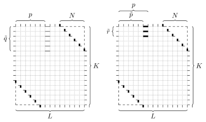
Figure 19. Constraints corresponding to the EFP (left) and AFP (right) in terms of non-intersecting lattice path. Here $L=15$, $M=25$, $N=6$, $p=7$, $q=8$, and therefore $K=17$, $\tilde{q}=6$, $\tilde{p}=6$, $\tilde{r}=3$.

We now resort to Prop. 7. With no loss of generality, we may restrict to $p\leq L-N$, see (4.3), that is, $\tilde{l}=N$, and set $\tilde{n}=\max(N-p,0)$. We get

$$F_{L,M,N}(p,q)=\frac{C_{L,M,N;p}}{Z_{L,M,N}}\sum_{\tilde{n}<\mathbf{y}\leq K-\tilde{q}}\,\prod_{\tilde{n}<i<j\leq N}(y_{j}-y_{i})^{2}\prod_{i=\tilde{n}+1}^{N}\tilde{\mu}(y_{i}),$$ (C.2)

where $\tilde{\mu}(y)$ is given by $\mu(y)$ in (B.2), but with $n$ and $\tilde{l}$ replaced by $p$ and $N$, respectively. Relabelling and shifting the variables, $y_{i}\to x_{i+\tilde{n}}+\tilde{n}+1$, and observing that

$$\tilde{\mu}(x+\tilde{n}+1)=w_{K-\tilde{n}-1}^{(p-N+2\tilde{n},L-N-p)}(x),$$ (C.3)

we finally get

$$F_{L,M,N}(p,q)=$$ (C.4)

$$=\frac{C_{L,M,N;p}}{Z_{L,M,N}}\sum_{0\leq\mathbf{y}\leq K-\tilde{q}-\tilde{n}-1}\,\prod_{1\leq i<j\leq N-\tilde{n}}(y_{j}-y_{i})^{2}\prod_{i=1}^{N-\tilde{n}}w_{K-\tilde{n}-1}^{(p-N+2\tilde{n},L-N-p)}(x_{i})$$ (C.5)

$$=H(K-\tilde{n}-\tilde{q}-1,p-N+2\tilde{n},L-N-p,N-\tilde{n},K-\tilde{n}-1),$$ (C.6)

where the function $H(\cdot)$ has been defined in (4.11). Recalling that $\tilde{q}=p+q-L+N$, $K=M-L+N-1$, we recover Prop. 4. ∎

Let us now turn to the proof of Prop. 5.

Proof.

We want to show that AFP may be expressed in terms of EFP, via a suitable identification of the parameters. We shall resort once again to the bijection between configurations of the four-vertex model and non-intersecting lattice paths.

As already observed, the definition of EFP, namely that, in the hexagonal domain, the topmost $\tilde{q}=p+q-L+N$ vertices in the $p$th vertical line are all of type $a$, once rephrased in terms of non-intersecting lattice paths, reads: on the $L\times K$ lattice, no path flows through the topmost $\tilde{q}$ horizontal edges, in the $p$th column. Similarly, the definition of AFP implies the flow of a path through each of the $\tilde{r}$ topmost horizontal edges, in the $\tilde{p}$th column, where

$$\tilde{p}=p-\mathrm{mod}(\tilde{q}+1,2),\qquad\tilde{r}=\bigg{\lfloor}\frac{\tilde{q}+1}{2}\bigg{\rfloor}.$$ (C.7)

Indeed, the requirement that, in the hexagonal domain, the topmost $\tilde{q}$ vertices in the $p$th vertical line are all of type $c$, implies having a path flowing through each of the topmost $\tilde{r}$ horizontal edges to the right (and left) of the $p$th line when $\tilde{q}$ is odd (even), see Fig. 19.

Figure 20. An example of the procedure used to relate EFP and AFP. Starting from a give configuration of non-intersecting lattice paths, with frozen corners removed (top left), swap the states of all edges in the frozen triangular corners (top right), swap the state of all horizontal edges (bottom left), and shift all paths eastward, obtaining a four-vertex model configuration on a rotated $K\times M$ lattice with $K-N$ lines (bottom right). Here $L=15$, $K=17$, $N=6$, and hence $M=25$.

In order to express AFP in terms of EFP, we consider another bijection between configurations of the four-vertex model and non-intersecting lattice paths. For any given configuration of $N$ non-intersecting paths on the $L\times K$ rectangular domain, let us implement the following procedure i) swap the state (full/empty) of each edge in the northeast and southwest frozen triangular corners; in other words, in these two corners, paths are transformed from all vertical to all horizontal; this action does not change the number of allowed configurations; ii) swap the state of all horizontal edges; as a result, we have $K-N$ lattice paths; these may now osculate, but we assume they do not intersect, so that each path is still uniquely defined; iii) shift the $i$th path, $i=1,\dots,K-N$, enumerated from the top, by $K-N-i$ steps to the right. Note that, with the last step, the horizontal size of domain becomes $L+K-N-1=M$. An example of this procedure is given in Fig. 20.

All steps of the above procedure being invertible, it follows that each configuration of $N$ non-intersecting paths on the $L\times K$ rectangular domain is bijectively mapped into a configuration of the four-vertex model on the $K\times M$ domain (rotated by $\pi/2$), with $K-N$ lines.

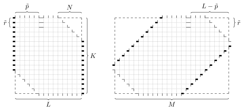
Figure 21. The AFP-constraint with inversed horizontal edges (left) and equivalent EFP-constraint (right).

Note that under this bijection the condition defining the AFP, namely the flow of a path through each of the $\tilde{r}$ topmost horizontal edges, in the $\tilde{p}$th column, becomes the condition of having only vertices of type $a$ within a rectangular region of size $\tilde{r}\times(L-\tilde{p})$ in the northeast corner of the $K\times M$ domain with $N-K$ lines, see Fig. 21. In formulae:

$$G_{L,M,N}(p,q)=F_{K,M,K-N}(\tilde{r},L-\tilde{p}).$$ (C.8)

Restoring the dependence from the original parameters, we recover Prop. 5. ∎

Finally, let us derive Prop. 6.

Proof.

It follows from Prop. 4 and Prop. 5 that AFP may be written according to (4.16), with parameters

$$d=\min(\tilde{r},M-L+1)-\tilde{r}+\tilde{p}-1,\qquad\alpha=\absolutevalue{M-L-\tilde{r}+1},\qquad\beta=N-\tilde{r},$$ (C.9)

$$s=\min(\tilde{r},M-L+1),\qquad n=L-N+\min(\tilde{r},M-L+1)-1.$$ (C.10)

Noting that $2\tilde{r}-\tilde{p}=\tilde{q}-p+1$, implying $L-N+\tilde{r}-\tilde{p}=q+1-\tilde{r}$, we recover expression (4.17) for the parameters. ∎