Consistent Causal Inference for High-Dimensional Time Series††thanks: We are grateful to the Editor Serena Ng and the Referees for comments that have led to corrections and improvements in content and presentation. We are also grateful to Yanqin Fan for having shared the latest version of Fan et al. (2022) and useful discussions. We thank the participants at the Model Evaluation and Causal Search workshop at the University of Pisa, the Lancaster Financial Econometrics Conference in honour of Stephen Taylor, and the 2023 SoFiE Conference at Sungkyunkwan University. The first author acknowledges financial support from MIUR Progetti di Ricerca di Rilevante Interesse Nazionale (PRIN) Bando 2017. Both authors acknowledge financial support from the Leverhulme Trust Grant Award RPG-2021-359.
Abstract
A methodology for high dimensional causal inference in a time series context is introduced. It is assumed that there is a monotonic transformation of the data such that the dynamics of the transformed variables are described by a Gaussian vector autoregressive process. This is tantamount to assume that the dynamics are captured by a Gaussian copula. No knowledge or estimation of the marginal distribution of the data is required. The procedure consistently identifies the parameters that describe the dynamics of the process and the conditional causal relations among the possibly high dimensional variables under sparsity conditions. The methodology allows us to identify such causal relations in the form of a directed acyclic graph. As illustrative applications we consider the impact of supply side oil shocks on the economy, and the causal relations between aggregated variables constructed from the limit order book on four stock constituents of the S&P500.
Key Words: high dimensional model, identification, nonlinear model, structural model, vector autoregressive process.
JEL Codes: C14, G10.
1 Introduction
Identifying and estimating causal relations is a problem that has received much interest in economics. In the last two decades the statistical and machine learning literature has made a number of advances on the front of identification and estimation within the framework of causal graphs (Comon, 1994, Hyvärinen and Oja, 2000, Pearl, 2000, Spirtes et al., 2000, Hyvärinen et al., 2001, Shimizu et al., 2006, Meinshausen and Bühlmann, 2006, Kalisch and Bühlmann, 2007, Cai et al., 2011, Bühlmann et al., 2014, Peters et al., 2014), where the data generating process can be characterized as a system of structural equations. This complex causal relations system might be represented through the causal graph, which conveys essential topological information to estimate causal effects.
However, the true data generating process is often a latent object to researchers, which can only rely on finite sample observations to infer the causal structure and mechanism of the true system. A causal model entails a probabilistic model from which a researcher can learn from observations and outcomes about changes and interventions of the system variables (Pearl, 2000, Peters et al., 2014). Thus, causality can be formally defined using the do-notation of Pearl (2000) in terms of intervention distributions. This definition of causality is quite different from the well known concept of Granger causality. However, causal relations in economics and finance require to account for time series dependence.
In this paper we develop a methodology to extract the causal relations of time series data, conditioning on the past in a flexible way. We assume that there is a monotone transformation of the data that maps the original variables into a Gaussian vector autoregressive (VAR) model (see also Fan et al., 2022). There are a number of advantages to this approach. First, we are able to retain the interpretability of VAR models building on the rich econometrics literature on structural VAR models. Second, we do not need any assumptions on the marginal distribution of the data. This means that the procedure is robust to fat tails, as we do not make any assumption on the existence of any moments. For instance, given that the existence of a second moment for financial data has been a much debated topic in the past (Mandelbrot, 1963, Clarke, 1973, for some of the earliest references) dispensing all together of this unverifiable condition should be welcomed. Third, we can model variables that take values in some subset of the real line, for example variables that only take positive values or are truncated. This is not possible using a standard VAR model.
The estimation of the contemporaneous causal structure of a time series is equivalent to solving the identification problem of a structural VAR model. The latter can be achieved by finding a unique Choleski type decomposition of the covariance matrix of the VAR innovations (Rigobon, 2003, Moneta et al., 2013, Gouriéroux et al., 2017, Lanne et al., 2017). Recent advances in the identification problem under general conditions and linearity exploit the use of internal and external instruments and the method of local projections (Stock and Watson, 2018, Plagborg-Møller and Wolf, 2021). However, the time series dynamics of economic and financial data may not be captured well by a linear VAR model when the data is not Gaussian. For example, some variables may only be positive. The problem of estimation is exacerbated if the data have fat tails. This may distort the estimates. Such problems reflect negatively on the estimation of causal relations for time series data. Furthermore, due to the curse of dimensionality, SVAR analysis is only feasible in a low-dimensional context. Restricting the VAR model only to a few variables may lead to unreasonable adverse effects such as ‘price-puzzles’ in impulse responses (Sims, 1992, Christiano et al., 1999, Hanson, 2004). Moreover, models of the global economy tend to be high dimensional. To avoid the curse of dimensionality, factor augmented VAR (FAVAR) models (Bernanke et al., 2005) and dynamical factor models (Forni et al., 2000, Forni et al., 2009) are often employed. However, the interpretation of the causal relations with factor models is not always straightforward. Along these approaches, we also mention the GVAR methodology, originally proposed by Pesaran et al. (2004), where country specific VAR models are stacked together in a way that maintains ease of interpretation at the cost of some assumptions. Our methodology does not require the machinery of factor models or assumptions on how to join lower dimensional models into a higher dimensional one. However, this is achievable at the cost of certain restrictions. We envisage that our methodology could work in conjunction with the the existing ones to shed further light on structural relation in high dimensional VAR models. We also point out that high dimensional VAR models may even arise in practice as a result of a large number of lags.
This paper builds on a number of previous contributions and develops a methodology to address the aforementioned problems. Our approach is tantamount to the assumption that the cross-sectional and transition distribution of the variables can be represented using a Gaussian copula. The procedure builds on the work of Liu et al. (2012) and does not require us to estimate any transformation of the variables or the marginal distribution of the data, as commonly done when estimating a copula. In fact, our procedure bypasses the estimation of the innovations of the model altogether. Our methodology is built for high dimensional time series, as commonly found in some economics and financial applications. What we require is some form of sparsity in the partial dependence of the data. This is different from assuming that the covariance matrix of innovations or the matrix of autoregressive coefficients are sparse. Such two restrictions can be restrictive. We shall make this clear in the text when we discuss our assumptions. Finally, even when not all causal relations are identified, we are able to identify the largest number of causal relations. This statement is formalized by the concept of complete partially acyclic graph using the PC algorithm (Spirtes et al., 2000, Kalisch and Bühlmann, 2007). These concepts are reviewed in the main body of the paper (Section 3).
We conclude this introduction with a few remarks whose aim is to put the goals of this paper into a wider perspective. The process of scientific discovery is usually based on 1. the observation of reality, 2. the formulation of a theory, and 3. tests of that theory. The plethora of data available allows the researcher to observe different aspects of reality that might have been precluded in the past. High dimensional estimation methods are particularly suited to explore the present data-centric reality. However, the next step forward requires formulation of a theory or hypothesis. Such theory needs to be able to explain rather than predict in order to enhance our understanding. This very process requires the identification of a relatively small number of explanatory causes for the phenomenon that we are trying to understand. The problem’s solution, in a complex and rather random environment, should then be a simple approximation. This approximation can then be tested in a variety of situations in order to verify its applicability. The program of this paper is to follow this process of scientific discovery. We start from possibly high dimensional dynamic datasets. We aim to provide a reduced set of possible contemporaneous causes conditioning on the past.
1.1 Relation to Other Work
One of the main empirical econometric tools for the study of policy intervention effects is the VAR approach (Sims, 1980, Kilian and Lütkepohl, 2017). In the first step, the so called reduced form model is estimated. Then, the structural counterpart needs to be recovered. This gives rise to an identification problem, which is equivalent to finding the contemporaneous causal relations among the variables.
Traditionally, the identification of Structural Vector Autoregressive (SVAR) models was achieved by imposing model restrictions. Such restrictions can be derived from an underlying economic model, such as short and long-run restrictions on the shocks impact (Bernanke, 1986, Blanchard and Quah, 1989, Faust and Leeper, 1997), or imposing sign restrictions on impulse response functions (Uhlig, 2005, Chari et al. 2008).
The success of the VAR approach is its reliance on data characteristics, thus allowing the validation of economic models under reasonably weak assumptions. However, standard restrictions necessary for the identification invalidate the data-driven nature of SVAR. Recently, researchers have explored alternative methods to achieve identification in SVAR models by exploiting different statistical features of the data. For instance, identification can be obtained by relying on heteroskedasticity (Sentana and Fiorentini, 2001, Rigobon, 2003, Lütkepohl and Netšunajev, 2017) or non-Gaussianity of the residuals (Moneta et al., 2013, Gouriéroux et al., 2017, Lanne et al., 2017). On the other hand, another popular method used for identification, which however does not exploit specific statistical properties of the data distribution as the previously mentioned, is the instrumental variables approach (Mertens and Ravn, 2013, Stock and Watson, 2018, Plagborg-Møller and Wolf, 2021).
Our method is related to approaches that rely on the graphical causal model literature (Swanson and Granger, 1997, Demiralp and Hoover, 2003, Moneta, 2008), where identification can be achieved by exploiting the set of conditional and unconditional independence relations in the data. Our work is also related to the statistical and machine learning literature for the identification of causal graph structures in a high dimensional setting (Meinshausen and Bühlmann, 2006, Kalisch and Bühlmann, 2007, Liu et al., 2009, Zhou et al., 2011, Bühlmann et al., 2014, Harris and Drton, 2013). In particular the latter reference combines the use of rank correlations with the PC algorithm, as we do in the present paper. However, none of these approaches accounts for contemporaneous causal inference conditioning on the past, as required for time series problems.
To account for the time series dependence, we employ a modelling assumption that can be viewed as a Gaussian copula VAR model, a definition that will be made clear in the text. We recently discovered that Fan et al. (2022) have used the same time series assumption for the analysis of high dimensional Granger causality. The present paper is concerned with conditional causal relations and identification of the Gaussian copula VAR. Moreover, some basic assumptions are also different. For example, Fan et al. (2022) assume that the autoregressive matrix of the Gaussian copula VAR is sparse. We instead assume that the inverse of the scaling matrix of the Gaussian copula that leads to a VAR representation is sparse. This is a very different assumption. Hence, the contributions are related, but complementary.
1.2 Outline of the Paper
The plan for the paper is as follows. In Section 2, we introduce the model and briefly discuss its statistical properties. In Section 3 we discuss identification of the model and the causal relations. In Section 4 we describe algorithms to find estimators for the population quantities, including the complete partially acyclic graph. In Section 5 we state conditions and results for the consistency of the quantities derived from the algorithms. Section 6 provides two empirical illustrations. First, we investigate the identification of the effect of supply side shocks on economic activity. Then, we analyze the causal relations of order book variables in electronic trading. Section 7 concludes. Additional explanatory material can be found in the Appendix. There, we provide more details on the model and its identification under possibly mixed data types. We also discuss calculation of impulse response functions for our nonlinear model. All the proofs and other additional details can be found in the Electronic Supplement to this paper. There we also present the main conclusions from a simulation study as evidence of the finite sample properties of our methodology (Section S.3 in the Electronic Supplement).
Software.
The algorithms presented in this paper are implemented in the R scripting language. The code is available from the URL https://github.com/asancetta/CausalTimeSeries. Most of the code is based on existing R packages and also includes a cross-validation procedure to choose tuning parameters.
2 The Model
Let be a sequence of stationary random variables taking values in or some subset of it. For each , we suppose that there is a monotone function such that is a standard Gaussian random variable such that
| (1) |
where has singular values in and is a sequence of independent identically distributed random variables with values in and covariance matrix . Throughout, the prime symbol ′ denotes transposition. All vectors in the paper are arranged as column vectors. We do not require knowledge of the functions . We also note that there is always a monotone transformation that maps any univariate random variable into a standard Gaussian. We provide details about this in Section A.1 in the Appendix. Here, the main assumption is that such transformed variables satisfy the VAR dynamics in (1). Under stationarity assumptions, all the information of the model can be obtained from the covariance matrix of the -dimensional vector , which we denote by . We can then partition as
| (2) |
with obvious notation, once we note that is as in (1) and . Clearly, (recall ).
The above setup can be recast into a formal probabilistic framework using the copula function to model Markov processes (Darsow et al., 1992). The copula transition density would be the ratio of two Gaussian copulae: one with scaling matrix and one with scaling matrix . Given that we shall not use this in the rest of the paper, we omit the details. However, given this fact, for short, we refer to our model as a Gaussian copula VAR. We note that when has an invariant distribution with marginals that are continuous, the functions are necessarily equal to the unconditional distribution of , by Sklar’s Theorem (Joe, 1997).
We consider a high dimensional framework, where can go to infinity with the sample size. Formally, this would require us to consider a family of models (1) indexed by the sample size to allow for increasing dimension (Han and Wu, 2019, for more details). We do not make explicit this in the notation. Next, we summarise the main properties of the model under the possibility that .
Proposition 1
Define for some increasing monotonic transformation , , such that follows a Gaussian VAR as described in (1). Furthermore, suppose that the singular values of are in a compact interval inside and the eigenvalues of are in a compact interval inside , uniformly in . Then, is a stationary Markov chain with strong mixing coefficients that decay exponentially fast, uniformly in even for .
Recall that the singular values of a matrix are the square root of the eigenvalues of . Hence, the condition means that is full rank with eigenvalues inside the unit circle. We note that for fixed the model is not only strong mixing, but also absolutely regular (beta mixing), with exponentially decaying coefficients (Doukhan, 1995, Theorem 5, p.97). However, when is allowed to increase, this is not the case anymore (Han and Wu, 2019, Theorem 3.2). Nevertheless, allowing for increasing dimension , it is still strong mixing with exponentially decaying coefficients.
The extension of (1) to a VAR(), for fixed finite , has been considered by Fan et al. (2022, Appendix B). The process remains geometrically strong mixing if the singular values of the autoregressive matrices are all in a compact interval inside . For simplicity, we shall restrict attention to the VAR(1) case. The methodological implementation for a higher order VAR is simple, but we will still provide some remarks on this as it is relevant to the high dimensional framework.
3 Identification
In the next section, we briefly review causal graph terminology. While these concepts are not widely used in econometrics, they do simplify some discussion when stating assumptions and contemporaneous relations (Section 6.1 for an empirical illustration to oil price shocks). In Section 3.2 we show how these concepts relate to the more familiar language and setup of structural vector autoregressive models.
3.1 Preliminary Concepts
A graph consists of a set of vertices , where is the number of vertices, and edges . The edges are a set of ordered pairs of distinct vertices. The edges are directed if the order matters, but , otherwise it is undirected. Arrows are commonly used to define the direction when there is one. In our context, is the set of indices of , i.e. , while contains the direction in the causal relations if any. For example, we know that we cannot have while the other way around is possible if Granger causes . In the language of graphs we say that is a parent of . In this paper we focus on the causal relations of conditioning on . This is different from Granger causality. Given that the statistical relations of the elements in conditioning on are defined by , we focus on finding the set of parents of each . For example, is a parent of if causes and not the other way around. We write . When the variables are jointly Gaussian, it is well known that conditional independence is not enough to identify the direction of the relation (Moneta et al., 2013, Peters et al., 2014).
In the case when all causal relations are identified with no cycles, the causal graph is a directed acyclic graph (DAG): all edges are directed and there are no cycles. There are no cycles if no descendant can be a parent of their ancestor. When the direction cannot be fully identified, we shall content to obtain some undirected edges. It is possible that no directed edge can be identified. The graph where we do not consider the directions is called the skeleton. When we use observational data, we work with their distribution, possibly under model assumptions as in (1). We say that the distribution of the data is faithful to the graph if the set of all (possibly conditional) independence relations of the distribution of the data and the graph coincide. The (possibly conditional) independence relations of the graph are defined as the set of vertices for which there is no edge between them. Such relations only require to identify the skeleton. Unfortunately, a given distribution of data can generate an infinite number of DAG’s. In the case of a VAR this is equivalent to say that the structural VAR cannot be identified. This means that we cannot draw arrows for all edges. Hence, we may need to content ourselves with a complete partially directed acyclic graph (CPDAG), which is a graph where some edges are undirected because they cannot be identified. In summary, in the more familiar language of econometrics, identification of the DAG of the -dimensional innovations means that the system of simultaneous equations for is recursive. This is equivalent to finding a permutation of the variables such that the covariance matrix of the permuted innovations is the product of a lower triangular matrix times its transpose (Lemma 2 in Section 3.2). We shall use a sample based version of the PC algorithm (Kalisch and Bühlmann, 2007) to identify the CPDAG under the assumption that the underlying causal structure is recursive. For high dimensional time series data, we require special tools as devised in the present paper.
3.1.1 Remarks on the PC Algorithm
A full description of the PC algorithm can be found in (Spirtes et al., 2000). Here, we provide a short overview assuming knowledge of . The PC algorithm identifies as many causal relations as possible and its output is a CPDAG. In the present case, it exploits the assumption that the system of simultaneous equations of the innovations is recursive (i.e. the causal graph is a DAG). It then proceeds into two steps. The first step exploits the set of all conditional independence relations in the data as follows. It identifies the so called moral graph, which is the set of all edges implied by the nonzero entries in . Note that the entry in is zero if and only if and are independent when conditioning on all other variables (Proposition 5.2 in Lauritzen, 1996). Using the zero entries in , it removes all those edges in the moral graph that correspond to variables that are unconditionally independent, i.e. independent when conditioning on the empty set. This produces the skeleton. It then uses a set of logical rules to direct as many arrows as possible.
We give a straightforward example of identification strategy used by the PC algorithm. Suppose that we only have a set of three variables . Suppose that any pair of variables from this set is dependent when conditioning on the third one. According to the aforementioned remarks on , we have that this matrix has no zero entries. However, suppose that when we condition on the empty set, and are independent. This means that these two variables are unconditionally independent. This is tantamount to saying that and entries in are zero. In this case, we must have that and are related to each other only through a common effect . The PC algorithm would then produce the following DAG . This conclusion does not assume that the underlying causal structure be representable by a DAG. Other logical rules used by the PC algorithm assume that the causal relations between the variables be representable by a DAG (Algorithm 2 in Kalisch and Bühlmann, 2007, for the full list of rules).
In the next section, we relate these concepts to SVAR identification and existing methods based on instruments. We do so to show how our methodology adds to the arsenal of already existing methods.
3.2 Identification of the Gaussian Copula VAR
We conclude with two results that show the identification strategy in our methodology. We define the precision matrix . As we did for in (2), we partition it with same dimensions as in (2):
| (3) |
The parameters in (1) are identified from the precision matrix (3). The following, is a consequence of the classical result on graphical Gaussian models (Lauritzen, 1996, eq. C3 and C4).
Lemma 1
Suppose that the conditions of Proposition 1 hold. Then, and .
When the DAG is identified, we can identify the SVAR. In the more common language used in econometrics, this is the same as saying that the structural equation system of the innovations is recursive, as it will be formally defined in (6). To this end, we introduce some notation. Let be a matrix that can be transformed into the identity by simple permutation of its rows. We call a permutation matrix as it permutes the rows of the conformable matrix that it premultiplies. We have the following result for identification of the SVAR.
Lemma 2
Suppose that the conditions of Proposition 1 hold and that the causal graph for in (1) is a DAG. Then, we can find a permutation matrix such that
| (4) |
where is lower triangular with diagonal elements equal to zero, and is a vector of independent Gaussian random variables such that is a diagonal full rank matrix. In particular, the innovation in (4) satisfies where is a full rank lower triangular matrix with diagonal elements equal to one. Furthermore, the process admits the infinite moving average representation
| (5) |
From the causal DAG we can derive the permutation matrix , where each row describes the recursive order of the nonzero entry in such row. The ordering is often nonunique. In what follows, we shall always refer to the matrix as the one that is obtained from the least number of row permutations of the identity matrix. In this case is unique. Hence, estimation of the DAG is equivalent to estimation of the permutation matrix . From Lemma 2 we deduce that
| (6) |
where the above is a structural equation system for the innovations . The variables on the right hand side are the cause of the left hand side variables.
From the structural model in (4) it is clear that the shock specific to is the entry in , using the fact that . By this remark and (5), the impact on of intervening on (via the entry in ) is computed as where is the vector of zeros, but for the entry, which is one. Given that the structural shock has diagonal matrix with possibly different diagonal elements, we may use in place of , where . It is clear that the representation in (5) in terms of the shocks is not sufficient to carrying out causal inference in the sense of the structural equation system (6). Knowledge of the permutation matrix is necessary. Working with observational data, we start from a reduced form model (1) and obtain (4) when identification is possible. In turn, identification is only possible if can be identified.
When interest lies on the impulse response functions, we need to account for nonlinearity. The model in (1) is linear only after applying a transformation to each variable. Koop et al. (1996) address such problem focusing on generalized impulse response functions for reduced form models (Kilian and Lütkepohl, 2017, Ch.18 for a discussion on structural models). An explicit discussion on the calculation within our framework can be found in Section A.2 of the Appendix. However, by linearization, the impulse response function is approximately equal to a constant multiple of (Lemma A.2 in the Appendix, and discussion therein).
3.2.1 Identification Using External Instruments
The identification strategy based on the PC algorithm (Section 3.1), is one additional method to be added to the arsenal of existing strategies based on internal and external instruments, possibly using local projections (Stock and Watson, 2018, Plagborg-Møller and Wolf, 2021). This follows from the fact that the latent VAR in (1) is Gaussian. Hence, expectations and projections are just functions of in (3). The latter is one of the quantities of interest in this paper.
We note that the methodology based on external instruments can have nontrivial implications for a recursive system, when projections and conditional expectations coincide, as in the Gaussian case. Suppose an augmented VAR so that an external instrument is included in the VAR as first variable to identify the effect of a shock of on . Being an instrument, satisfies the usual instrumental variable exclusion assumption for a SVAR (Assumption LP-IV in Stock and Watson, 2018, Assumption 4 in Plagborg-Møller and Wolf, 2021). Adapting Assumption 4 in Plagborg-Møller and Wolf (2021) to our notation and using the Markov assumption implied by (1), this means that conditional on takes the form for some constant (Plagborg-Møller and Wolf, 2021, Eq.17). Note that is the structural shock of variables . Then, from (6) we know that . Substituting the latter in the former equation, we have that
| (7) |
Given that for Gaussian random variables zero correlation is equivalent to independence, the above is a structural equation. In particular it means that is caused by all the variables in for which the vector has nonzero entries. The simplest case is when is not caused by any other entry in . In graph language, this means that is a source node and in structural equation notation it means that . From (6), this can only be the case if is a zero row vector.
The above shows that the standard representation (7) for the instrumental variable exclusion assumption for a SVAR has non trivial implications in empirical work. In fact, given that (7) is a structural equation, means that , the instrument conditioning on the past, must be caused by and possibly by other variables. This is contradictory to the empirical interpretation of an instrument. In one of our empirical illustrations, we consider the oil supply shock identification methodology discussed in Känzig (2021). There the instrument is based on price changes around OPEC announcements. The variable of interest for which we want to measure the effect of a shock is real oil prices. When projections and conditional expectations coincide, (7) essentially implies that OPEC announcements () are contemporaneously caused by real oil price () and possibly other variables. This is contrary to what is usually put forward as a justification for the use of this instrument. Of course, projections and conditional expectations may be unrelated, and more importantly the system may not be recursive. Nevertheless, we shall show that an approach based on structural equations (and equivalently causal graphs) can help us understanding the underlying assumptions.
Suppose that satisfies (6). The exclusion restriction using an instrument where is standard normal can instead be formulated as where is conditioning on the past of and is a structural shock independent of . Then, is a valid instrument if is a structural shock. This means that is a structural shock when we omit . To see this, note that satisfies the IV exclusion restriction for the impact of on the other variables, and it is compatible with a recursive structural equation system. Assuming that (1) holds for the augmented vector that also includes , we can recover the joint distribution of and , and apply any of the projection methods used in the literature. Our methodology allows us to do this. Moreover, relying on a sample version of the PC algorithm, we can also estimate whether this exclusion restriction holds for the augmented dataset. We shall illustrate this in Section 6.1 with the dataset in Känzig (2021). In summary, our framework not only puts forward an alternative identification approach, but also allows us to use existing methodologies. Relying on causal graphs and structural equations systems can allow us to precisely define assumptions, and its visual aspect may help our intuition.
Next, we introduce algorithms that will be shown to produce consistent estimators, under assumptions stated in Section 5.2.
4 Estimation Algorithms
For any positive integer , . For any matrix of dimensions and sets and , is the submatrix with rows in and columns in . In , when we write and similarly if . When for some , we write and similarly for . When is a vector, it is always assumed that it is a column vector and we shall use the same notation, but with one single subscript. This notation will be used throughout the paper with no further mention.
The estimation methodology is based on a number of steps which extend the methodology in Liu et al. (2012). First, we find an estimator of the matrix in (2), which is the Gaussian copula scaling matrix of the vector . This is achieved using Algorithm 1. Once, the estimator for is available, we identify the set of zero entries in the precision matrix, i.e., the inverse of . This can be achieved using Lasso, as described in Algorithm 2. This algorithm follows the approach of Meinshausen and Bühlmann (2006) to find the zeros in the inverse of (2). However, the algorithm also thresholds the resulting Lasso estimators in order to achieve sign consistency. In this form, the algorithm is equivalent to Gelato (Zhou et al., 2011).
In Algorithm 2, (8) is solved by the that satisfies the first order conditions in a Lasso minimization problem. The constraint is needed to avoid running the regression of the variable on all the other covariates and itself. We need the estimator to be in this form for later use. A competing algorithm to find the zeros of the precision matrix is the CLIME estimation algorithm with thresholding (Cai et al., 2011). The procedure is described in Algorithm 3. The minimization problem in Algorithm 3 can be solved for one column of at the time, with as defined there, due to the use of the uniform norm. We shall show the validity of both algorithms within the time series context of this paper.
Algorithm 4 allows us to estimate the parameters in (1). In particular, it uses the information on the zeros of the estimator for the precision matrix to construct a sparse estimator (Le and Zhong, 2021). Using Lemma 1, such sparse estimator of the precision matrix is used to estimate the autoregressive matrix and the covariance matrix of the innovations in (1).
Finally, using Algorithm 5, we identify the PCDAG. Algorithm 5 makes reference to the PC algorithm. We do not report the details in Algorithm 5, as the number of steps is relatively large and can be found in Spirtes et al. (2000) among many other places. The aim of the PC algorithm is to start with a dense graph with undirected edges for all variables. It then aims at removing edges to obtain the skeleton of the graph. Finally, it uses a set of rules to direct all possible edges based on deterministic rules. It is not guaranteed that all edges can be directed, of course.
In order to delete edges, the PC algorithm uses the correlation coefficients between two variables, conditional on subsets of other variables. Note that the innovations in the latent model (1) are Gaussian so that zero correlation implies independence. As soon as we find a set of conditioning variables such that the two variables are conditionally uncorrelated, we remove an edge between these two variables. Given that the conditional correlations are unknown, Kalisch and Bühlmann (2007) suggest to replace these with sample versions as in Algorithm 5. They define a parameter , as in Algorithm 5, and show that for at a certain speed we can obtain a consistent estimator of the PCDAG, as if we knew the true conditional correlations. For this reason, Algorithm 5 only gives details on the sample estimator leaving out the deterministic steps, to avoid distracting details.
Identification of the SVAR requires that all edges are directed. Assuming that Algorithm 5 can direct all the edges, for each , we obtain estimators for the set of parents of , using the notation in Algorithm 6. According to Lemma 2, to find the matrix , we need to find the regression coefficients of the innovation on , . Algorithm 6 finds such regression coefficients and collects them into a matrix , . In particular, the row of has entries equal to the coefficients found regressing on and zeros elsewhere. By the fact that the graph is a DAG, there is a permutation matrix such that is an estimator for and is a lower triangular matrix with zeros along the diagonal. The regression coefficients are obtained relying on . This is because is a sparse estimator with good asymptotic properties. Such properties are inherited by even though is not sparse. The estimator is not necessarily sparse. Moreover, regression coefficients are found directly from with no need to estimate the innovations.
Set .
Run Algorithm 1 to obtain .
For :
Denote by the solution to
| (8) |
Redefine as .
Let be a neighbour of if .
For each :
Set equal to , but let , where is the entry.
Set .
Run Algorithm 1 to obtain .
Let be the solution to s.t. .
Redefine as and denote by the column of the redefined .
Let be the subvector obtained by deleting the zero elements in and denote by its size.
Denote by the matrix such that
Define where is the vector with entry equal to one and zero otherwise.
Let .
Denote by the entries in , .
Denote by the entries of with , and .
Define as an estimator for in (2).
Define as an estimator for .
Run Algorithm 4 to find .
Use to find the estimator of the correlation coefficient of and conditioning on where is a set that excludes . Denote such correlation coefficient by .
Use the PC algorithm (Spirtes et al., 2000) and delete a node between if where () and .
Run Algorithm 5 and suppose that the PC algorithms identifies the DAG in the sense that it produces and estimator for the true edges , such that all elements in are directed.
For :
Find all such that so that conditioning on the , the covariate is a parent of the one (i.e. ). Denote such set by .
Find .
Let be the matrix such that and zero otherwise.
Find the matrix obtained from the least number of row permutations of the identity matrix and such that is lower diagonal with diagonal elements equal to zero.
The tuning parameters for Algorithms 2 and 3 are chosen using cross-validation (Section S.2 in the Electronic Supplement, for details).
In the Electronic Supplement, we also use simulations to investigate the finite sample properties of the estimators in our algorithms (see Section S.3 in the Electronic Supplement).The simulation analysis show that our approach produces more reliable results than methods that do not account for either sparsity or time series dependence, i.e. setting in Algorithms 2 and 3 or assuming in (1). Even when the persistence of the time series is reduced, our methodology produces the best results for estimation of the causal structure and the VAR parameters (for details, see Tables S.1-S.6 in Section S.3 in the Electronic Supplement). Although our approach is designed for a high dimensional setting, it provides competitive results even in the low dimensional case.
5 Asymptotic Analysis of the Algorithms
The consistency of the algorithms relies on a set of conditions. Before introducing our conditions, we introduce some additional notation.
5.1 Additional Notation
For any vector, the norm is denoted by , . For any dimensional matrix , is the elementwise norm. When we define . When both we simply write , and this should not cause confusion with the norm. For , . When , this is just the total number of non-zero elements in . Finally, is used to define the following operator norm: . Then, is the largest singular value of . For ease of reference, we call this norm the operator’s norm.
Let
| (9) |
The symbol is used to mean that is a symmetric strictly positive definite matrix. Then, is the set of symmetric strictly positive definite matrices whose absolute sum of column entries is at most , and with maximum number of non-zero entries in each row equals .
We shorten left and right and side with l.h.s. and r.h.s., respectively. Finally, is used when the l.h.s. is bounded above by a constant times the r.h.s.; is bounded below by a constant times the r.h.s.; is used when the l.h.s. is bounded below and above by constants times the r.h.s.. Finally, to avoid notational trivialities, we assume that .
5.2 Assumptions
Assumption 1
(Model) There are monotone functions such that is a standard Gaussian random variable such that (1) holds. Moreover, has continuous marginal distributions.
Assumption 2
(Dimension) The state space is a subset of , where for some .
Assumption 3
(Precision matrix sparsity) The precision matrix is an element of for for some .
Assumption 4
(Identifiability) , , where is the smallest absolute value of the nonzero elements in .
Assumption 5
(Eigenvalues) The singular values of are in a compact interval inside and the eigenvalues of are in a compact interval inside , uniformly in .
Strictly speaking, if as , we should index both the process and its law by and think in terms of a sequence of processes. We refrain to do so for notational simplicity. No part in the proofs makes implicitly use of assumptions that contradicts this.
5.3 Remarks on the Assumptions
Assumption 1.
The modelling assumption includes a Gaussian linear vector autoregressive model as special case. However, it is clearly more general than that. Once, we assume that the data satisfy a VAR model after a monotone transformation, we do not need to impose any moment condition on the original data. Hence the procedure is robust to fat tails. As discussed in Section 2, we can view this assumption as a Gaussian copula assumption for the cross-sectional and time series dependence. Assumption 1 can be viewed as a generalization of the framework of Liu et al. (2012) in the time series direction and has been recently exploited by Fan et al. (2022) to test for Granger causality in high dimensional models.
The continuity of the marginal distribution of is not needed. As shown in Fan et al. (2017) we can recover the parameters of the latent Gaussian process even for mixed data types (see also Section A.1 in the Appendix). In this case, we would modify Algorithm 1 accordingly.
Our results apply to a VAR() for fixed and finite , if we redefine to be ; here is defined locally and not related to the same symbol in other parts of the paper. Then, we just need to change the dimension of the set of matrices in (9) from to where . The conditions, will then apply to these new quantities. Clearly, the dimension of the matrix is while the dimension of the submatrix in (3) is still .
Assumption 3.
The precision matrix is supposed to have maximum absolute sum of each column bounded by a constant . Our bounds make explicit the dependence on so that we can have if needed. This constant is only used in Algorithms 2 and 3. The total number of non zero elements in each row is supposed to be bounded by a constant . This is allowed to grow to infinity with the sample size at a certain rate. This assumption is different from Fan et al. (2022) who assumes that the autoregressive matrix in (1) is sparse. This is not the case here. By Lemma 1, sparsity of does not imply sparsity of either or . In order to see this, we recall that if and only if and are independent, conditioning on all the other remaining variables Lauritzen (1996, Proposition 5.2), where .
Example 1
For random variables , let mean that and are independent given . Now, suppose that for all and ,
and
and such that . Intuitively, this means that variables that are not close to each other in terms of index are conditionally independent. The intersection with is to avoid conditioning on for example, as we only have variables. Given our modelling assumption (1), and the previous remarks about , this means that and are tridiagonal. Moreover, means that the partial correlation between and given all other covariates (including ) is the same as the partial correlation between and given all other covariates (including ) is the same. From Lemma 1 and the fact that the inverse of a tridiagonal matrix is not sparse, we deduce that both and are not sparse.
Clearly, we can obtain non-sparse from sparse under more general setups than Example 1. This is just chosen as a simple illustration for the sake of conciseness.
Assumption 4.
This assumption is only used to ensure that we can identify the zero entries in . It is necessary in order to ensure the validity of post selection asymptotic, though the rate can be arbitrarily slow when (Leeb and Pötscher, 2005, p.29ff).
Assumption 5.
The eigenvalues condition means that the variables are linearly independent in the population. This could be weakened, but at the cost of technical complexity. This assumption also implies the following.
Lemma 3
Under Assumption 5 the following statements hold uniformly in :
-
1.
The eigenvalues of are bounded away from zero and infinity;
-
2.
There are constants such that the eigenvalues of in (2) are in the interval ;
-
3.
There is a such that ;
-
4.
The partial correlations of and conditioning on any other subset of remaining innovations is bounded above by a constant .
5.4 Uniform Convergence of the Scaling Matrix Estimator
The uniform consistency of the covariance estimator from Algorithm 1 is well known (Liu et al., 2012). It is still consistent for dependent data.
Theorem 1
Under the Assumptions, .
Fan et al. (2022) show a similar result using Kendall’s tau instead of Spearman’s rho with a different method of proof.
5.5 Estimation of the Undirected Graph
5.5.1 Consistency for Algorithm 2
The reader is referred to the Assumptions and Algorithm 2 for the notation. Let be the population regression coefficient including a zero in the entry, i.e. the solution to s.t. .
Theorem 2
One could choose slowly enough, in which case the bound would be instead of . The proof of this result shows that we could have stated the results as finite sample one with high probability. However, such statement would still depend on an unknown constant. Hence, for simplicity, we have chosen not to do so.
Using appropriate thresholding, with threshold constant greater than the noise level, but smaller than , the absolute value of the smallest nonzero entry in , leads to set identification. In what follows is the sign of the real variable with .
5.5.2 Consistency Results for Algorithm 3
The reader is referred to the Assumptions and Algorithm 3 for the notation.
Theorem 4
The same remark we made about in Theorem 2 applies here. Also here, we could have stated the result as a finite sample one with high probability.
Using the appropriate level of thresholding, Theorem 4 implies the following.
5.6 Estimation of the Process Parameters and Causal Graph
In what follows, we suppose that the conditions of either Theorem 3 or Theorem 5 hold, depending on which algorithm is used. For short we generically refer to these as the Assumptions as they also involve restrictions on the choice of penalty and threshold .
5.6.1 Consistency of Precision Matrix Estimation
The estimator for the precision matrix is elementwise uniformly consistent under sparseness conditions.
Theorem 6
Suppose that the Assumptions hold. Then, the estimator from Algorithm 4 satisfies .
5.6.2 Consistency of the Estimators for the Autoregressive Matrix and Innovation Covariance Matrix
Recall that by Lemma 1, using the notation in (1) and (3), and . Hence, we need consistency of and the inverse of , which is the case under sparseness. Recall that as in Assumption 3. We have the following bounds in terms of the operator’s norm.
Theorem 7
Suppose that the Assumptions hold. Then, and .
5.6.3 PC Algorithm
Let be the estimated PCDAG from Algorithm 4 and the true PCDAG. The next result requires faithfulness of the distribution of the data to the graph, as defined in Section 3.1. In what follows, is the cumulative distribution function of a standard normal random variable.
Theorem 8
Theorem 8 says that the estimator for the PCDAG converges to the true one at an arbitrarily fast polynomial rate. This is worse that the exponential rate obtained by Kalisch and Bühlmann (2007) for causal discovery using independent identically distributed data.
5.6.4 Consistency of Structural Model Parameters
We show that from Algorithm 6 is consistent for , with as in Lemma 2. When the PC algorithms in Algorithm 5 produces edges that are all directed, we interpret to be the one corresponding to the permutation matrix that is obtained by the least number of row permutations of the identity. Then, is unique.
In the following, we state the consistency of for , and the consistency of an estimator for , in (5), with convergence rates. We shall denote by the maximum number of direct descendants among all parents. It is not difficult to show that this is the same as the maximum number of nonzero elements among the columns of . Such number is bounded above by , which corresponds to the maximum number of adjacent variables across all the nodes.
Theorem 9
Suppose that the Assumptions hold, that the joint distribution of the innovations in (1) is faithful to the DAG for all , and that all the estimated edges resulting from Algorithm 5 are directed. Then, using Algorithm 6, , where is as in (4) with obtained by the least number of row permutations of the identity. Moreover, we also have that satisfies .
6 Empirical Illustrations
To showcase the methodology presented in this paper we consider two illustrations. The first considers a supply side oil price shock. This problem has recently been considered by Känzig (2021). While the baseline model used in Känzig (2021) only includes 6 variables, this is still a high dimensional problem due to the fact that the selected number of lags is 12. Our aim is to highlight the features of our methodology and how it can be used to gain additional insights on the role of an external instrument. This application should clarify some of the language used in the paper and draw a clear parallel between the more common language used in economics and causal DAG’s. We hope to convince the reader that the use of the DAG has much to offer, once its role is understood.
The second application focuses on the causal relation between information in the order book in high frequency trading. For this application, the latent model is a VAR(1), however, the number of variables is large: . Among other things, there we highlight how the information from the impulse response functions produces a net effect that is different from the causal information flow represented by the structural equation model or equivalently the causal graph.
6.1 The Effect of Oil Price Shocks
Shocks in real oil price can be caused by either demand or supply shocks. Känzig (2021) uses oil futures price changes around OPEC announcements as an instrument to identify supply side shocks. We use our methodology to show how we identify the latent structural VAR model without an instrument for this specific dataset. We then include the instrument as an additional variable to our model and show that the resulting DAG suggests that this is a valid instrument, though unnecessary for the purpose of identifying the structural parameters. We stress that the goal of this application is to refer to a state of the art approach for a well known problem and show what we can achieve with our methodology, assuming that the system is recursive.
6.1.1 The Data and the Covariates
We consider the same dataset used in Känzig (2021). The data consists of real oil price, U.S. CPI, U.S. industrial production, world industrial production, world oil inventories and world oil production. We also include a Crude Oil Shock variable constructed in Känzig (2021), as additional variable. This variable can be used as either internal or external instrument for identification. Here, it will be used as an internal instrument to show that it is a valid instrument, relying on the graphical method of the paper. The sample period is from February 1975 to December 2017. The data is at monthly frequencies. Due to either the persistency or nonstationarity of the data, we first difference all variables except for the oil supply news shock. The covariates are listed in Table 1.
| Name | Short Name | |
|---|---|---|
| Crude Oil News Shock | OilShock | |
| Real Oil Price | OilPrice | |
| World Oil Production | WorldOilProd | |
| World Oil Inventories | WorldOilInv | |
| World Industrial Production | WorldIndProd | |
| U.S. Industrial Production | UsIndProd | |
| U.S. CPI | UsCpi |
6.1.2 Estimation
We estimate the causal graph using our proposed methodology and the six variables introduced in the previous section. We allow for lags greater than one, by the minor modification discussed in Section 5.3. We choose a lag length of 12 as in Känzig (2021). This is in line with the choice by Akaike’s information criterion as implemented in Section S.2.1 of the Electronic Supplement. We use both Lasso (Algorithm 2) and CLIME (Algorithm 3) for the estimation of the sparse precision matrix. For these algorithms, the penalization parameter and the threshold parameter are selected using cross-validation (see Section S.2 in the Electronic Supplement for details). We then apply Algorithms 4, 5, and 6 to estimate the Gaussian copula VAR parameters, recover the contemporaneous causal structure and possibly identify the matrix of contemporaneous relations . The latter can then be used for estimation of the impulse response functions.
6.1.3 Summary of Results
The results for Lasso and CLIME were very similar. In the interest of space, we report and discuss only the results when Lasso (Algorithm 2) is used as intermediate step, with no further mention.
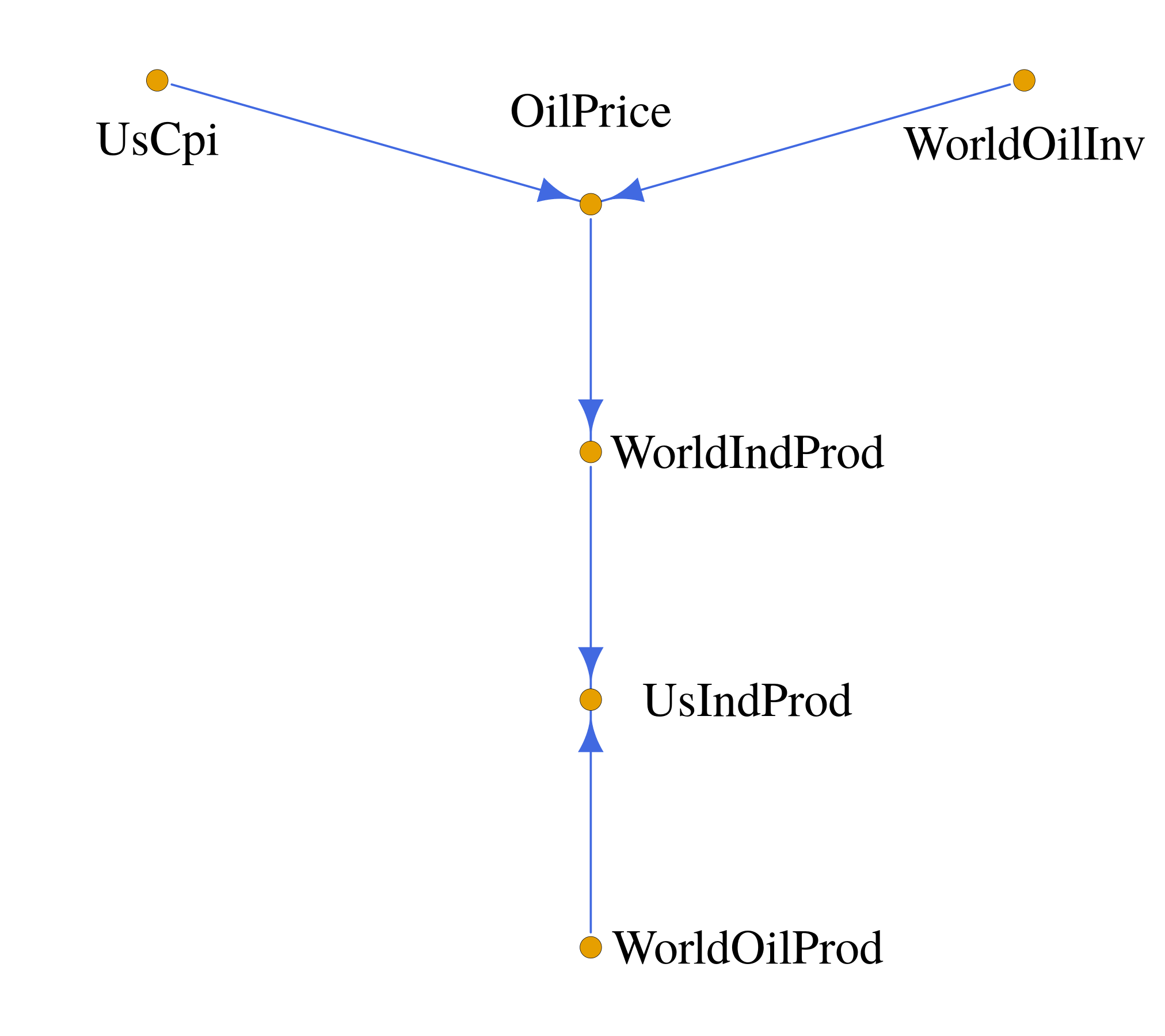
Using our methodology, we estimate a model with 12 lags, in line with Känzig (2021). This means that the number of relevant parameters to be estimated is , where is the number of covariates in the model without instrument. Given a sample size of we clearly are in a high dimensional setting. We found that all the edges of the causal graph were directed. This means that we are able to identify the permutation matrix and the matrix in Lemma 2. In consequence, the SVAR parameters are identified without the need of an instrument, under the assumption that the system is recursive. We report the DAG in Figure 1.
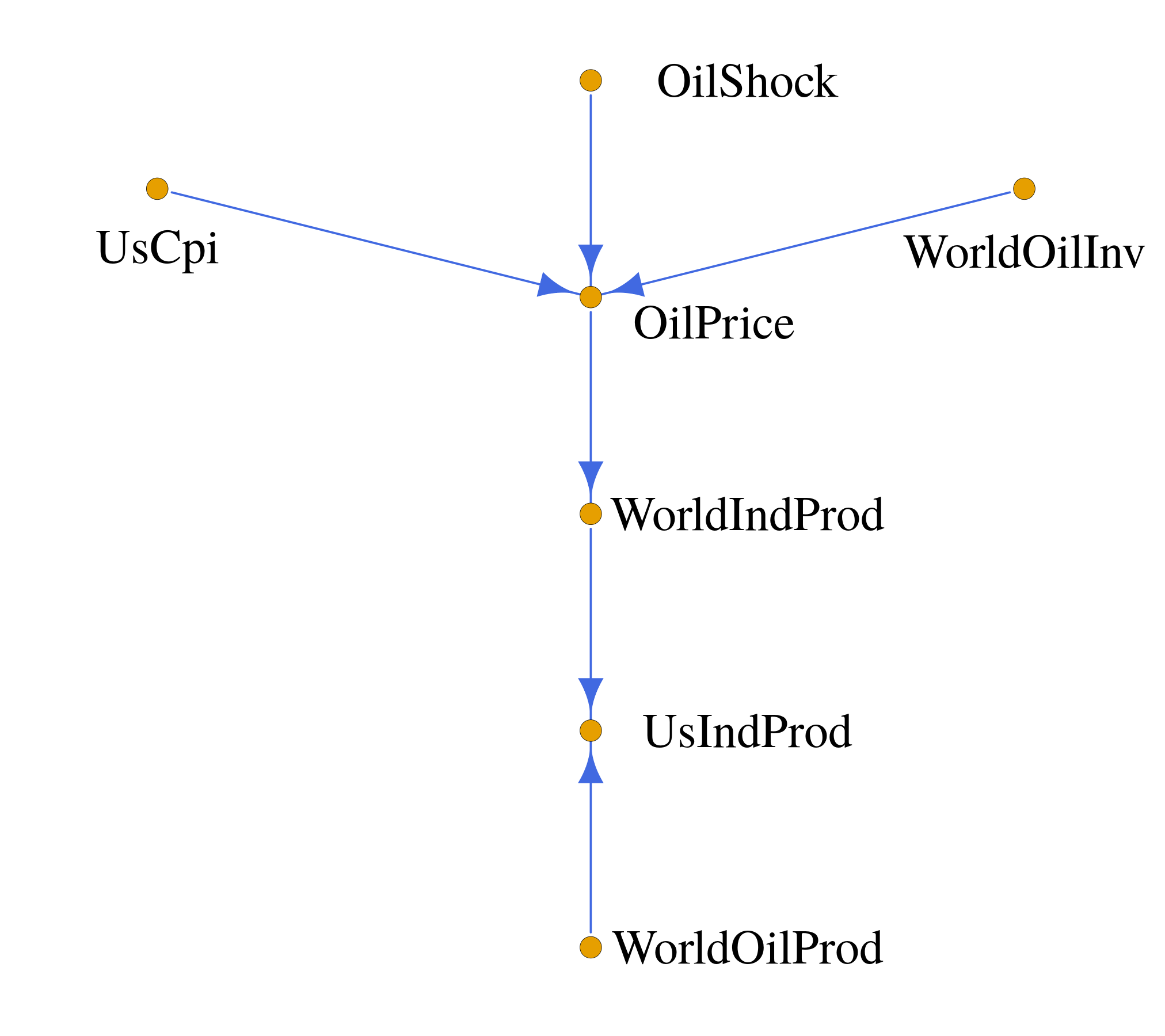
To shed further light on the value of OilShock as instrument used in Känzig (2021) and confirm that it satisfies the exclusion restriction for an instrument, we estimate the model including the latter as an additional variable. We now have variable with same number of lags. The result shows that OilShock is a source node, it impacts real oil prices directly and is not connected to any of the other variables. According to the discussion in Section 3.2.1 this means that it is a valid instrument.
The results also highlight a challenge. We find that a shock to UsCpi leads to a contemporaneous effect on OilPrice. This appears inconsistent with logic and economic theory. One explanation is that the underlying assumption that the system is recursive, after proper permutation, is not satisfied. However, the direction of this particular causal relation is identified using the example at the end of Section 3.1, which does not rely on recursivity. To see this, note that from the data we have that OilShock and UsCpi are unconditionally independent, but dependent when we condition on OilPrice. Then, this implies that OilShock and UsCpi are unrelated common causes to OilPrice (Section 3.1). Hence, the answer needs to be found elsewhere. To check that the results are not statistical artifacts specific to our methodology, we estimate the same model as in Känzig (2021): a VAR for the levels of the observed variables with 12 lags. We then check whether the residuals of OilShock and UsCpi are unconditionally independent of each other and all other variables, but are dependent when conditioning on OilPrice. We found that with 95% confidence, this is the case. Hence, we rule out that this is a statistical artifact specific to our methodology. The answer requires work beyond the scope of this paper.
There are two take away from this empirical illustration. First, for this specific data set, we are able to identify the latent SVAR parameters, under the assumption of a recursive structure with no need for an instrument. Note even assuming that the structure is recursive, the set of possible solutions has cardinality that grows exponentially with the number of variables. Hence, this is a nontrivial exercise. Second, by including the potential instrument as one of the variables, we are able to confirm the validity of the instrument. Again the underlying assumption is that the system is recursive. However, given the structure of the graph, recursivity is not used to orient the edges in the subgraph OilPrice, OilShock and UsCpi.
(a)
(b)
6.2 Causal Relations in the Limit Order Book
Large orders to buy or sell stocks in a financial market are usually broken into smaller ones and executed over a fixed time frame, where time can be measured in clock time or volume time (Donnelly, 2022 for a review). One important dilemma when executing orders is to decide whether to execute crossing the spread or posting passive orders. The latter does not guarantee immediate execution. However, it is believed to reduce market impact. Empirical evidence shows that passive orders that skew the limit order book also cause market impact. Hence, it is of interest to understand the causal implication of an algorithm that keeps posting limit orders resulting on an order book imbalance (Table 2 for definition) versus an algorithm that continuously trade crossing the spread. Moreover, limit orders may be posted at deeper levels in to book to gain queue priority. Such actions tend to have a persistent impact on the book as many orders need to be executed over a finite number of time. We are interested in understanding the implications of such persistent actions.
To this end, we apply our methodology to study the causal relations between aggregated order book and trades variables in high frequency electronic trading. Aggregation allows us to reduce noise and extract information that is concealed at high frequency. We aggregate the information in volume time (Section 6.2.1, for more details). This is different from the analysis of order book tick data which has been studied extensively in the literature (Cont et al., 2014, Kercheval and Zhang, 2015, Sancetta, 2018, Mucciante and Sancetta, 2022a, 2022b). It is well known that market participants look at the order book to extract market information (MacKenzie, 2017). We want to extract average causal relations. The underlying assumption is that (6) holds, i.e. the causal structure can be represented in terms of a DAG.
We shall estimate a model with 5 stocks to investigate the direction of information dissemination within each stock, via the order book and trades, as well intra stocks. This requires the estimation of a large dimensional model. Our results will also show how the methodology of this paper allows us to disentangle contemporaneous causal effects from time series effects.
6.2.1 The Data and the Covariates
We consider four stocks constituents of the S&P500 traded on the NYSE: Amazon (AMZN), Cisco (CSCO), Disney (DIS) and Coca Cola (KO). We also consider the ETF on the S&P500 (SPY). The stock tickers are given inside the parenthesis. The sample period is from 01/March/2019 to 30/April/2019, from 9:30am until 4:30pm on every trading day. The data were collected from the LOBSTER data provider (Huang and Polak, 2011)111https://lobsterdata.com/.. This is a Level 3 dataset, meaning that it contains all limit orders and cancellations for the first 10 levels of the order book as well as trades, all in a sequential order.
We construct a set of covariates related to the ones that are commonly found in the studies of high frequency order book and trades. However, we use aggregated data in volume time in intervals of 10% of daily volume of SPY. Volume time means that instead of clock time, we use cumulated trades as measure of time. We choose SPY as common time for all the instruments as this is the asset that replicates the S&P500 index. Aggregated data allow us to estimate an average propensity of each covariate to cause the other. For example, an order book where limit orders to buy tend to be much higher than limit orders to sell could drive the price up over. The covariates are the book imbalance up to ten levels, a geometric average return, and the trade imbalance, often termed order flow imbalance. The covariates are listed in Table 2, where their definition can be found. In Table 2, and is the from the previous minute bucket, where is the ask price at level and similarly for . The operator takes the data from the same one minute bucket and computes the average value. In case of much market activity, the exchange will use the same timestamp for a number of messages at different levels. In the case of the orderbook, we use the last book snapshot of the many with the same time stamp. We do not apply this logic to trades. These covariates are directional ones. For this reason, we have omitted other interesting ones, such as the spread. Moreover, the instruments we use are all very liquid and the spread does not change much in this case.
For ease of reference, in what follows, we shall use the convention of merging the ticker and covariate short name.
| Name | Short Name | Definition | |
|---|---|---|---|
| Book imbalance | |||
| at level | |||
| Return | |||
| Trade Imbalance |
6.2.2 Estimation
6.2.3 Summary of Results
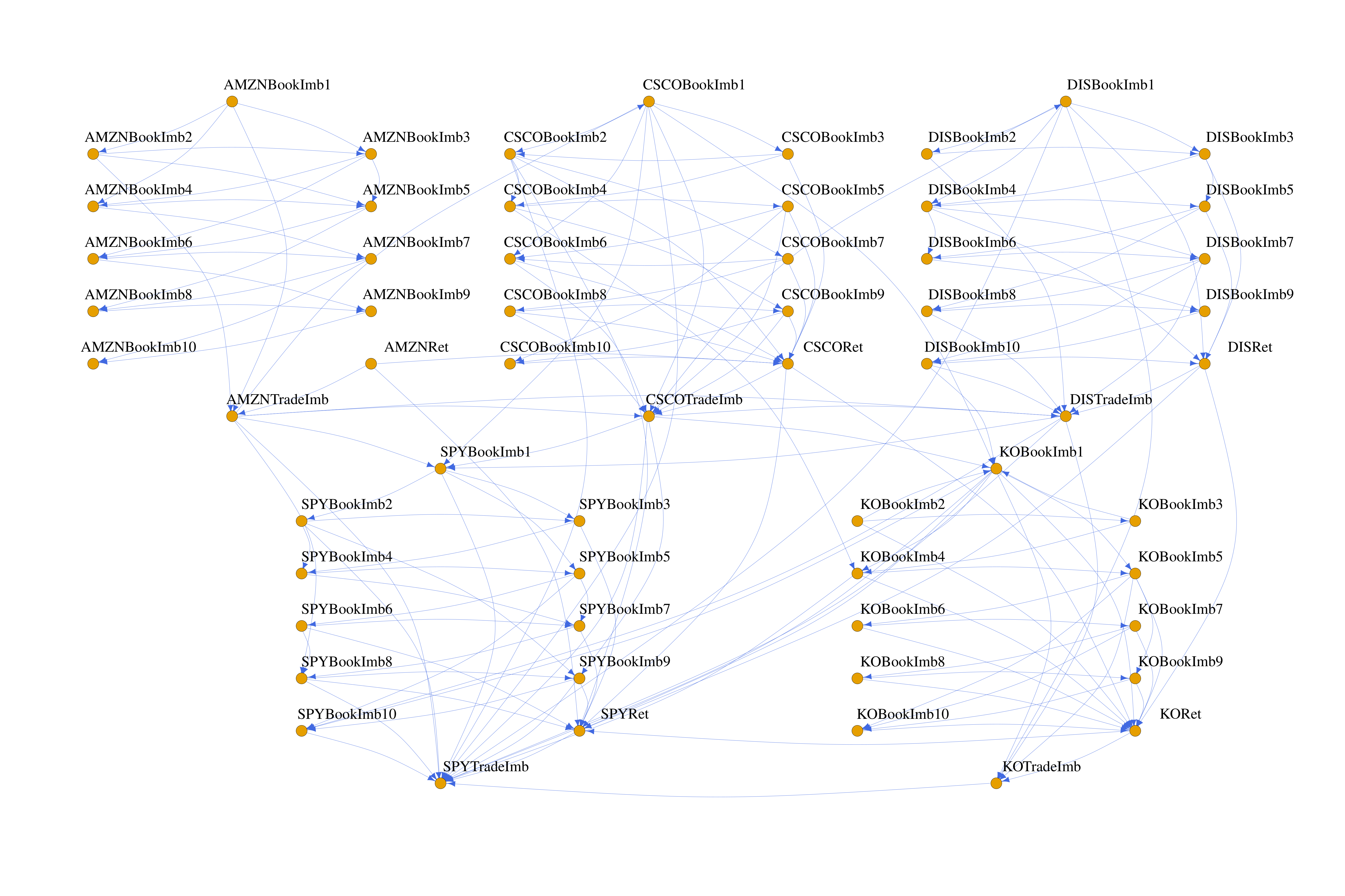
The results for Lasso and CLIME were very similar. We discuss only the results when Lasso (Algorithm 2) is used as intermediate step. Our results show that the causal structure of the order book of each instrument exhibits a dense network structure. Within each instrument, the first level of order book imbalance is not contemporaneously caused by any other variable (this is called a source node). In general we observe how the causal structure goes from top levels of the book to deeper ones. Usually, the return is affected directly by the deeper levels of the order book imbalance. For all instruments the return is a cause of the trade imbalance variable that does not happen to cause any other variable (this is called a sink node). We also observe cross-causal effects across instruments. We observe how in general the return of an instrument could be affected by other instrument returns, e.g., AMZN return impacts CSCO and the SPY return. In particular, the SPY return is affected by the other returns. We also observe that the trade imbalance of an instrument may directly affect the top levels of the book of other instruments impacting so on all the order book structure, e.g., the AMZN trade imbalance directly affects the first level of CSCO and SPY book imbalance as well as the respective trade imbalance together with trade imbalance of DIS and the eighth level of the SPY book imbalance.
The details can be found in Figure 2 that shows the DAG of contemporaneous causal relations obtained from our estimation procedure.
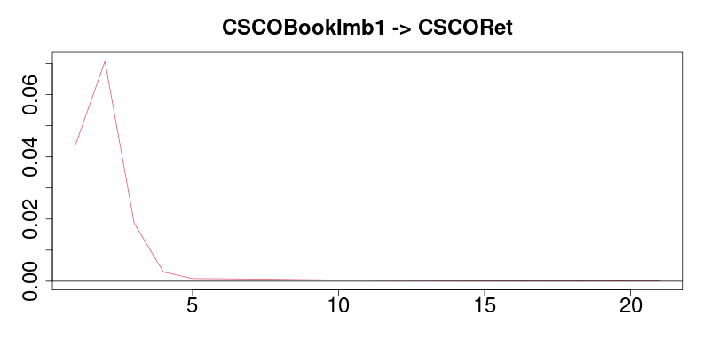
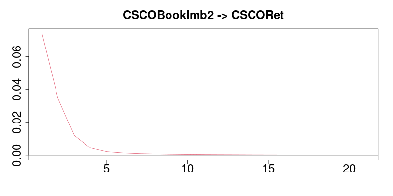
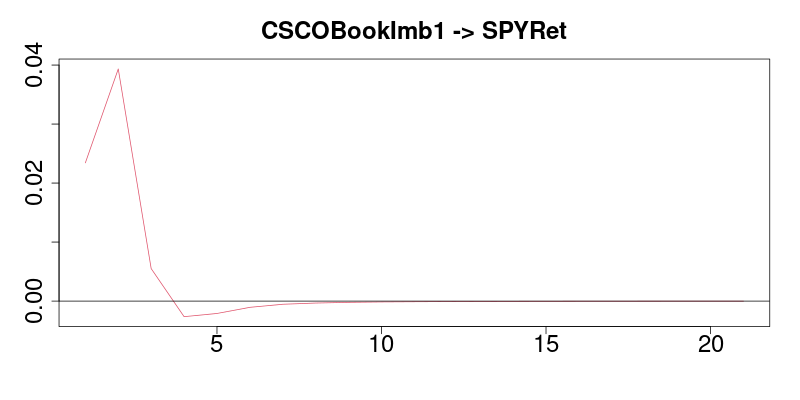
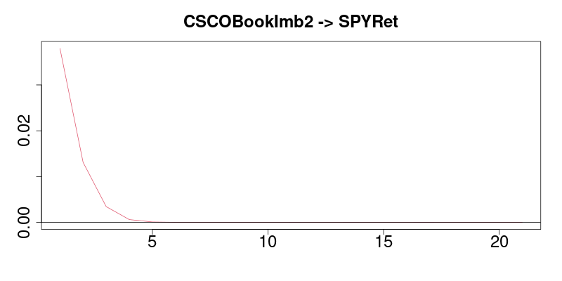
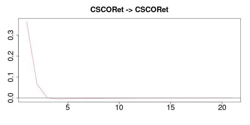
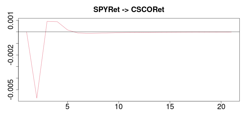
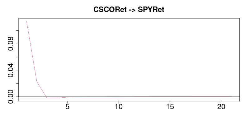
We also show how the contemporaneous impulse response function may fail to show the direct contemporaneous causal relations defined via in (6). Consider the subgraph composed by , , and as shown in Figure 3. The related impulse response functions are plotted in Figure 4.222Bootstrap confidence intervals were very tight due to the large sample size, so they are not plotted. By looking at the impulse response functions, we may conclude that and are directly affecting and . However, this effect is mediated as shown in Figure 3. There, we observe that a shock on will first impact the and and then it propagates to the . Only the causal graph or equivalently the structural equations system allows us to understand the information flow in the order book. The impulse response functions only represent the contemporaneous net effect of a shock.
(a)

(b)
7 Conclusion
This paper has introduced a novel approach for the estimation of causal relations in time series. It essentially uses a Gaussian copula VAR model. Such causal relations differ from Granger causality. Our methodology, allows us to identify causal relations in high dimensional models. Using a sparsity condition we are able to consistently estimate the model parameters. Our sparsity condition does not impose sparsity of the autoregressive matrix and of the covariance matrix of the innovations implied by the Gaussian copula VAR model. Our sparsity conditions can be viewed as weak assumptions on conditional independence. We are then able to identify the related directed acyclic graph of causal relations, using observational data, as if we knew the true distribution of the data.
Asymptotic results and finite sample investigation confirm the viability of our methodology and its practical usefulness for high dimensional problems. A finite sample analysis, carried out using simulation (Section S.3 in the Electronic Supplement), confirms the asymptotic results of the paper. Moreover, the simulations show that not accounting for time series dependence leads to wrong causal inference. Failing to exploit sparsity leads to suboptimal results, even in low dimensions.
We also relied on two empirical applications to highlight the methodology of the paper. We considered the effect of oil price shocks to the economy as studied in Känzig (2021). We showed how our methodology can be used to verify whether an instrument is needed and whether the instrument is a valid one. Then, we applied our methodology to the analysis of the conditional contemporaneous causal relations of order book data aggregated in volume time. To the best of our knowledge this has not been done before and has important implications for understanding the aetiology of electronic trading. The applications also showed how causal inference provides the path followed by a shock via a system of structural equations that has a graphical representation. On the other hand the contemporaneous impulse response functions show the net effect with no information on the actual causal path.
There are a number of areas that have been overlooked and require further research in the future. For example, the methodology assumes that the system of structural innovations of the latent VAR process is recursive. In this case, strategies for partial identifications within our framework need to be devised. However, we showed that methods based on instruments can still be used in our setup. Moreover, the literature has put forward the possibility of models that exhibit some form of time variation. This time variation is then exploited for identification via heteroskedasticity. Our framework does not cover this, yet. This extension requires careful study, as it has nontrivial implications for the meaning of causality, as used in this paper. For example, time variation may result from omitted variables/causes. In this case, a nonlinear framework, such as ours, can be a suitable starting point to address the problem. To conclude, our approach provides an opportunity for much new research building on the existing contributions in the literature.
References
- [1] Acid, S. and L.M. de Campos (2003) Searching for Bayesian Network Structures in the Space of Restricted Acyclic Partially Directed Graphs. Journal of Artificial Intelligence Research 18, 445–490.
- [2] Bernanke, B. (1986) Alternative Explanations of the Money-Income Correlation. In Carnegie-Rochester Conference Series on Public Policy 25, 49-99. North- Holland.
- [3] Bernanke, B.S., J. Boivin and P. Eliasz (2005) Measuring the Effects of Monetary Policy: A Factor-Augmented Vector Autoregressive (FAVAR) Approach. The Quarterly Journal of Economics 120, 387-422.
- [4] Blanchard, O. and D. Quah (1989) The Dynamic Effects of Aggregate Demand and Supply Disturbances. American Economic Review 79, 655-673.
- [5] Bühlmann, P., J. Peters and J. Ernest (2014) CAM: Causal Additive Models, High-Dimensional Order Search and Penalized Regression. The Annals of Statistics 42, 2526-2556.
- [6] Cai, T., W. Liu and X. Luo (2011) A Constrained Minimization Approach to Sparse Precision Matrix Estimation. Journal of the American Statistical Association 106, 594-607.
- [7] Chari, V., P.J. Kehoe and E.R. McGrattan (2008) Are Structural VARs with Long-Run Restrictions Useful in Developing Business Cycle Theory?. Journal of Monetary Economics 55, 1337-1352.
- [8] Christiano, L.J., M. Eichenbaum and C. L. Evans (1999) Monetary Policy Shocks: What Have We Learned and to What End?. Handbook of Macroeconomics 1, 65–148.
- [9] Clarke, P.K. (1973) A Subordinated Stochastic Process Model with Finite Variance for Speculative Prices. Econometrica 41, 135-155.
- [10] Comon, P. (1994) Independent Component Analysis a New Concept?. Signal Processing 36, 287–314.
- [11] Cont, R., A. Kukanov and S. Stoikov (2014) The Price Impact of Order Book Events. Journal of Financial Econometrics 12, 47-88.
- [12] Darsow, W.F., B. Nguyen and E.T. Olsen (1992) Copulas and Markov processes. Illinois Journal of Mathematics 36, 600-642.
- [13] Demiralp, S. and K.D. Hoover (2003) Searching for the Causal Structure of a Vector Autoregression. Oxford Bulletin of Economics and Statistics 65, 745-767.
- [14] Donnelly, R. (2022) Optimal Execution: A Review. Applied Mathematical Finance 29, 181-212.
- [15] Doukhan, P. (1995) Mixing. New York: Springer.
- [16] Fan, J., H. Liu, Y. Ning and H. Zou (2017) High Dimensional Semiparametric Latent Graphical Model for Mixed Data. Journal of the Royal Statistical Society B 79, 405-421.
- [17] Fan Y., F. Han and H. Park (2022) Estimation and Inference in a High-dimensional Semiparametric Gaussian Copula Vector Autoregressive Model. Preprint.
- [18] Faust, J. and E.M. Leeper (1997) When Do Long-Run Identifying Restrictions Give Reliable Results?. Journal of Business & Economic Statistics 15, 345-353.
- [19] Forni, M., D. Giannone, M. Lippi and L. Reichlin (2009) Opening the Black Box: Structural Factor Models with Large Cross-Sections. Econometric Theory 25, 1319-1347.
- [20] Forni, M., M. Hallin, M. Lippi and L. Reichlin (2000) The Generalized Dynamic-Factor Model: Identification and Estimation. Review of Economics and Statistics 82, 540-554.
- [21] Gouriéroux, C., A. Monfort and J.-P. Renne (2017) Statistical Inference for Independent Component Analysis: Application to Structural VAR Models. Journal of Econometrics 196, 111-126.
- [22] Han, F. and W.B. Wu (2019) Probability Inequalities for High Dimensional Time Series Under a Triangular Array Framework. https://arxiv.org/abs/1907.06577v1.
- [23] Hanson, M. S. (2004) The “Price Puzzle” Reconsidered. Journal of Monetary Economics 51, 1385–1413.
- [24] Harris, N. and M. Drton (2013) PC Algorithm for Nonparanormal Graphical Models. Journal of Machine Learning Research 14, 3365-3383.
- [25] Hyvärinen, A., J. Karhunen and E. Oja (2001) Independent Component Analysis. Wiley, New York.
- [26] Hyvärinen, A. and E. Oja (2000) Independent Component Analysis: Algorithms and Applications. Neural Networks 13, 411–430.
- [27] Huang, R. and T. Polak (2011) LOBSTER: The Limit Order Book Reconstructor. School of Business and Economics, Humboldt Universität zu Berlin, Techenical Report.
- [28] Joe, H. (1997) Multivariate Models and Dependence Models. London: Chapman & Hall.
- [29] Kalisch, M. and P. Bühlmann (2007) Estimating High-Dimensional Directed Acyclic Graphs with the PC-Algorithm. Journal of Machine Learning Research 8, 613-636.
- [30] Känzig, D. (2021) The Macroeconomic Effects of Oil Supply News: Evidence from OPEC Announcements. American Economic Review 111, 1092-1125.
- [31] Kercheval, A.N., Y. Zhang (2015) Modelling High-Frequency Limit Order Book Dynamics with Support Vector Machines. Quantitative Finance 15, 1-15.
- [32] Kilian, L. and H. Lütkepohl (2017) Structural Vector Autoregressive Analysis. Cambridge University Press.
- [33] Koop, G., M.H. Pesaran and S.M. Potter (1996) Impulse Response Analysis in Non-Linear Multivariate Models. Journal of Econometrics 74, 119–147.
- [34] Lanne, M., M. Meitz and P. Saikkonen (2017) Identification and Estimation of NonGaussian Structural Vector Autoregressions. Journal of Econometrics 196, 288-304.
- [35] Lauritzen, S. L. (1996) Graphical Models. Oxford: Oxford University Press.
- [36] Leeb, H. and B. M. Pötscher (2005) Model Selection and Inference: Facts and Fiction. Econometric Theory 21, 21-59.
- [37] Liu, H., F. Han, M. Yuan, J. Lafferty and L. Wasserman (2012) High Dimensional Semiparametric Gaussian Copula Graphical Models. The Annals of Statistics 40, 2293-2326.
- [38] Liu, H., J. Lafferty and L. Wasserman (2009) The Nonparanormal: Semiparametric Estimation of High Dimensional Undirected Graphs. Journal of Machine Learning Research 10, 2295-2328.
- [39] Lütkepohl, H. and A. Netšunajev (2017) Structural Vector Autoregressions with Heteroskedasticity: A Review of Different Volatility Models. Econometrics and Statistics 1, 2-18.
- [40] MacKenzie, D. (2017) A Material Political Economy: Automated Trading Desk and Price Prediction in High - Frequency Trading. Social Studies of Science 47, 172-194 .
- [41] Mandelbrot, B. (1963) The Variation of Certain Speculative Prices. Journal of Business 36, 394-419.
- [42] Meinshausen, N. and P. Bühlmann (2006) High-Dimensional Graphs and Variable Selection with the Lasso. The Annals of Statistics 34, 1436-1462.
- [43] Mertens, K. and M. O. Ravn (2013) The Dynamic Effects of Personal and Corporate Income Tax Changes in the United States. American Economic Review 103, 1212-47.
- [44] Plagborg-Møller, M. and C.K. Wolf (2021) Local Projections and VARs Estimate the Same Impulse Responses. Econometrica 89, 955-980.
- [45] Moneta, A. (2008) Graphical Causal Models and VARs: An Empirical Assessment of the Real Business Cycles Hypothesis. Empirical Economics 35, 275-300.
- [46] Moneta, A., D. Entner, P. O. Hoyer and A. Coad (2013) Causal Inference by Independent Component Analysis: Theory and Applications. Oxford Bulletin of Economics and Statistics 75, 705-730.
- [47] Mucciante, L. and A. Sancetta (2022a) Estimation of a High Dimensional Counting Process Without Penalty for High Frequency Events. Econometric Theory: https://doi.org/10.1017/S0266466622000238.
- [48] Mucciante, L. and A. Sancetta (2022b) Estimation of an Order Book Dependent Hawkes Process for Large Datasets. Preprint.
- [49] Pearl, J. (2000) Causality: Models, Reasoning, and Inference. Cambridge, UK: Cambridge University Press.
- [50] Peters, J., J. M. Mooij, D. Janzing and B. Schölkopf (2014) Causal Discovery with Continuous Additive Noise Models. Journal of Machine Learning Research 15, 2009–2053.
- [51] Rigobon, R. (2003) Identification through Heteroskedasticity. The Review of Economics and Statistics 85, 777-792.
- [52] Sancetta, A. (2018) Estimation for the Prediction of Point Processes with Many Covariates. Econometric Theory 34, 598-627.89-107.
- [53] Sentana, E. and G. Fiorentini (2001) Identification, Estimation and Testing of Conditionally heteroskedastic Factor Models. Journal of Econometrics 102, 143-164.
- [54] Shimizu, S., P. O. Hoyer, A. Hyvärinen and A. Kerminen (2006) A Linear Non-Gaussian Acyclic Model for Causal Discovery. Journal of Machine Learning Research 7, 2003–2030.
- [55] Sims, C. A. (1980) Macroeconomics and Reality. Econometrica 48, 1-48.
- [56] Sims, C. A. (1992) Interpreting the Macroeconomic Time Series Facts: The effects of Monetary Policy. European Economic Review 36, 975–1000.
- [57] Spirtes, P., C. Glymour and R. Scheines (2000) Causation, Prediction, and Search. Boston: The MIT Press.
- [58] Stock, J. H. and M. W. Watson (2018) Identification and Estimation of Dynamic Causal Effects in Macroeconomics Using External Instruments. The Economic Journal 128, 917-948.
- [59] Swanson, N. R. and C.W. Granger (1997) Impulse Response Functions Based on a Causal Approach to Residual Orthogonalization in Vector Autoregressions. Journal of the American Statistical Association 92, 357-367.
- [60] Tsamardinos, I., L. E. Brown and C. F. Aliferis (2006) The max-min hill-climbing Bayesian network structure learning algorithm. Machine Learning 65, 31–78.
- [61] Uhlig, H. (2005) What are the Effects of Monetary Policy on Output? Result from an Agnostic Identification procedure. Journal of Monetary Economics 52, 381-419.
- [62] Zhou, S., P. Rütimann, M. Xu and P. Bühlmann (2011) High-dimensional Covariance Estimation Based On Gaussian Graphical Models. Journal of Machine Learning Research 12, 2975-3026.
Appendix
A.1 Remarks on the Gaussian Transformation
We provide some remarks on the model in order to clarify its applicability. For simplicity of exposition, suppose that the number of covariates and that there is no time series dependence (i.e. is a zero matrix). For any univariate random variable , there is always a monotonic increasing function such that is standard normal. For example, let and , . By stationarity, the probability is independent of . Define
| (A.1) |
If the variables are continuous with density with no atoms, . The purpose of this section is to consider the case where is not necessarily continuous and show that our methodology still applies. Once we state the following result, it will become clear how to discuss the case where the variables are time dependent.
Lemma A.1
Let and be uniform random variables in independent of and . The following hold.
-
1.
is a uniform random variable in and almost surely, .
-
2.
Let be the quantile function of the standard normal distribution. Then, is a standard normal random variable, .
-
3.
Define . Then, is a function of . If and are independent, and we have that
-
4.
Let and be uniform random variables in with Gaussian copula, and , . Let , then, .
-
5.
Let and be standard Gaussian with correlation coefficient . Let and , , and
where is expectation w.r.t. the marginal law of , . Then, the function is strictly increasing w.r.t. . Moreover , where is the bivariate distribution of two standard normal random variables with correlation equal to .
-
6.
Suppose that is an estimator for satisfying in probability, and that the data is ergodic. Then
in probability.
Lemma A.1 show how the transformation in (A.1) can be used construct uniform random variables in (Point 1). Once variables are uniform, we can obtain standard Gaussian random variables (Point 2). Points 1 and 2 also mean that we can choose in the definition of (1) such that . Spearman’s rho is a commonly used measure of dependence which is invariant under strictly monotone transformation. However, the population Spearman’s rho for the transformed variables depends on the dependence between and , i.e. . Hence, it is no unique. When , the transformation produces a Spearman’s rho through independent linear interpolations between the discontinuity points of the distribution functions of the two variables (Point 3). On the other hand, if the variables are continuous, the transformation produces produces uniform random variables with dependence structure that maps into the dependence structure of the latent process via a closed for expression (Point 4). However, discontinuities do not preclude us from identification of the correlation coefficient of the latent Gaussian variables (Points 5). All we need to do is to replace the map with . Mutatis mutandis, this observation has been made in Fan et al. (2017) and can be used for identification of the distributional parameters of the latent process when is not continuous.
Example 2
Suppose that and are binary random variables with values in and such that , . Suppose that their joint dependence is captured by a Gaussian copula. Then from Lemma A.1, and where are uniform random variables in with Gaussian copula with scaling matrix such that the entry is where . Moreover, from Lemma A.1 (Point 5), we have that,
By strict monotonicity w.r.t. , if we know and , , we can uniquely identify .
Knowledge of essentially hinges on knowledge of . A uniformly consistent estimator of the distribution function of the data assures that such quantity is consistently estimated (Point 6). A natural estimator for is the empirical distribution function based on a sample of size . In this case, the uniform convergence is exponentially fast (Lemma S.2 in the Electronic Supplement). We also note that with an additive error ,
is equal to the sample rank correlation coefficient (sample Spearman’s rho) because is the rank of variable , . This also means that if is discontinuous, we can use as an estimator of , where is the sample Spearman’s rho. See Fan et al (2017) for consistency when needs to be estimated.
A.2 Impulse Response Functions
Given that our model is Markovian, we define
| (A.2) |
to be the impulse response of to a shock in equal to and conditioning on a fixed value of . Recall that is not necessarily the shock corresponding to . The latter is given by the entry in . Integrating out w.r.t. the marginal distribution of (A.2) gives an unconditional impulse response function. We introduce some notation to simplify the statement of the details in what follows. For any matrix , let , , be the entry, the row and column respectively. If is a column vector, write for its entry.
Lemma A.2
Under the conditions of Lemma 2, for any scalar , in (A.2) we have that
| (A.3) |
where has entry , and equals except for the entry which is fixed to a value equal to .
Let . Then, for , (A.2) equals
Despite the possibly involved notation, the conclusions of Lemma A.2 are simple. To find the impulse response, we need to find the inverse of . This function is unknown. Our methodology to estimate the parameters of the latent SVAR does not require explicit knowledge of . However, if we want to compute (A.2) such knowledge is needed. An estimator can be based on the truncated inverse of the empirical distribution function (Liu et al., 2009). Given that the latent model is Gaussian with i.i.d. innovations, the expectation can be simply computed by Monte Carlo integration (Section A.2.1 for more details). According to Lemma A.1, using the notation therein, we have that . Finally, Lemma A.2 says that if we are interested in the infinitesimal effect of a shock, we can linearize (A.2). In this case, up to a proportionality constant, (A.2) is equal to . Hence, we are only interested in the shape of the impulse response, knowledge of is sufficient.
A.2.1 Monte Carlo Integration
From Lemma 2, . Define so that . For each of the variables simulate i.i.d. Gaussian random vectors with covariance matrix . Use a superscript to denote these simulated data, i.e. . The expectation in (A.3) is approximated by
To compute an unconditional impulse response function, we need to integrate out . To do so, we replace the above with
where the random vectors are Gaussian mean zero with covariance matrix as in (2).
Supplementary Material to “Consistent Causal Inference for High Dimensional Time Series” by F. Cordoni and A. Sancetta
S.1 Proofs
Throughout, we use to denote constants.
We also recall a property of symmetric strictly positive definite partitioned matrices. Let where is a partition of . Then, where
| (S.1) |
(e.g. Lauritzen, 1996, eq. B.2).
The conclusions from Lemma 3 will be used in a number of places. Hence, we prove this first.
S.1.1 Proof of Lemma 3
We prove one point at the time.
Proof of Point 1.
From the condition on , we have that . We note that
, where , and are the eigenvalue, the minimum and the maximum eigenvalue of the argument (Bhatia, 1996, eq. III.13, using induction). Moreover, we have that
and
To see this note that
and similarly for the lower bound and for . Given that the eigenvalues are in and the eigenvalues are in by assumption, we conclude that the eigenvalues of are bounded away from zero and infinity, uniformly in .
Proof of Point 2.
From the definition in (2), we have the following equality,
where, here, represents a matrix of zeros. From the assumption on and the fact that , we can use the definition of eigenvalues and, mutatis mutandis, the previous inequalities, from the proof of Point 1, to deduce the result.
Proof of Point 3.
From (S.1) and the definition of as variance of , we deduce that the element in is the inverse of the variance of conditioning on , all the other variables and their first lag. Given that the eigenvalues of are bounded away from zero, uniformly in , the random variables are not perfectly correlated. Hence there must be a constant as in the statement of the lemma.
Proof of Point 4.
The eigenvalues of are in some compact interval inside , uniformly in , by assumption. Hence, the innovation vector has entries that are not perfectly dependent. This means that no conditional correlation between any two variables can be equal to one, uniformly in .
S.1.2 Proof of Proposition 1
It is clear that the process is a stationary Markov chain. The mixing coefficients are invariant of monotone transformations of the random variables. Hence, we can consider the mixing coefficients of in (1). For the Gaussian VAR model in (1), Theorem 3.1 in Han and Wu (2019) says that the strong mixing coefficient for variables periods apart satisfies where is the square root of the ratio between the largest and smallest eigenvalue of . This ratio is bounded by Lemma 3. On the other hand, is the largest singular value of , which is smaller than one, uniformly in , by assumption. Hence, the strong mixing coefficients decay exponentially fast.
S.1.3 Proof of Lemmas 1 and 2
The conditions in Proposition 1 ensure that the model is stationary. We use this with no explicit mention in the following.
S.1.3.1 Proof of Lemma 1
S.1.3.2 Proof of Lemma 2
By the assumption of the lemma, all edges of the graph of are directed. There are also no cycles. Hence, there must be a permutation matrix of the elements in such that the element in is not a parent of the element. This implies the structure where is a lower triangular matrix with diagonal entries equal to one. Note that can have diagonal elements equal to one because we are not assuming that is the identity. The fact that the graph is acyclic means that is full rank. Otherwise, we would have a descendant that is an ancestor of itself. Now note that the inverse of a lower triangular matrix is also lower triangular. Moreover, if the matrix has diagonal elements equal to one, also the inverse has diagonal elements equal to one. Hence, we can write where is as in the statement of the lemma and obtain (4). To find the infinite moving average representation, rewrite (4) as where, here, is the lag operator. By assumption, can be inverted and has an infinite convergent series representation. Hence, we deduce (5) by standard algebra and the aforementioned remarks on .
S.1.4 Exponential Inequality for Spearman’s Rho
For simplicity, we use notation that is local to this section only. In this section we assume that are real valued stationary random variables with exponentially decaying strong mixing coefficients. We also assume that the variables have continuous distribution function and . As usual, we denote by and the empirical distribution. Let be the rank of variable and similarly for . In Hoeffding (1948, p.318) we have that the sample version of Spearman’s rho is defined to be
| (S.2) |
This same statistic is also used in Liu et al. (2012, proof of Theorem 4.1). Note that other versions of of sample Spearman’s rho can be defined. These would essentially be equal to the above up to an additive term. Their analysis can be treated in a way similar to what follows. For simplicity, we only focus on the above.
We recall the following Bernstein inequality from Merlevède et al. (2009) which we shall use twice.
Lemma S.1
Let be a sequence of mean zero, stationary random variables whose absolute value is uniformly bounded by , and with exponentially decaying strong mixing coefficients. Then, for and , there is a constant , depending on the mixing coefficients only and such that
A general main ingredient for our derivation of an exponential inequality for (S.2) is the following.
Lemma S.2
Under the assumptions of this section, choose a , and let for any . Then, there is a constant such that
Proof. We can always find a continuous monotone transformation for in the range of . Hence, given that , we can assume that for the purpose of the proof. Note that continuity of does not mean that is a continuous random variable. Using standard techniques, we replace the supremum by the maximum over a finite number of elements. We then apply Lemma S.1.
To do so, for fixed but arbitrary , we construct intervals , , such that for . The construction is as follows and similar to the one of the Lebesgue integral. Fix an arbitrary and divide the interval into intervals where such . Then, is the smallest integer greater than or equal to . Define variables as . Similarly, define variables as . It is not difficult to see that this construction has the aforementioned properties. Note that we can have equal to a singleton, i.e. , if there are discontinuities in and such discontinuities are larger than .
The following is a standard argument in the proof of the Glivenko-Cantelli Theorem (van der Vaart and Wellener, 2000, proof of Theorem 2.4.1). From the fact that and are monotonically increasing, we have that and for . Also recall that . In consequence,
using monotonicity and the fact that by construction. In consequence,
Hence, using the union bound,
Set . Apply Lemma S.1 with for arbitrary, but fixed , and . A similar inequality holds for . Hence, we deduce the final result.
Control of the quantity below will be shown to be essentially equivalent to control of (S.2).
Lemma S.3
Under the assumptions of this section, choose a , and let for any . Then, there is a constant such that
Proof. By the triangle inequality and the uniform boundedness of the empirical distribution function,
We apply Lemma S.2 to the first two terms on the r.h.s. and Lemma S.1 to the last one to deduce the result.
The definition of the population version of Spearman’s rho (e.g., Joe, 1997, p.32) between two random variables with joint distribution and marginals and is . Hence, we have the following.
Lemma S.4
Under the assumptions of this section, there is a constant such that for large enough and any ,
Proof. Dividing and multiplying by , (S.2) is equal to
Again, by simple algebra, the triangle inequality and the fact that has range in , we have that for large enough, e.g. ,
In consequence,
We can then apply Lemma S.3 with and to the r.h.s. of the above display. In Lemma S.3 for , we have which implies that . In Lemma S.3, replace its lower bound and upper bound in the numerator and denominator of the exponential function to deduce the result.
S.1.5 Lemmas on Control of the Sample Covariance Estimator and Related Quantities
To avoid notational trivialities, suppose that . If not, replace with in what follows. Recall that is the rank correlation between and . By stationarity, this does not depend on . We have the following.
Lemma S.5
Under the Assumptions, for large enough, there is a finite constant such that
Proof. This follows from the inequality in Lemma S.4. There, we set to deduce that for ,
for . Under the Assumptions, for large enough, . Substituting in the above display we find that the r.h.s. is bounded above by and this proves the lemma.
We now show that the correlation matrix obtained from Spearman’s rho converges.
Lemma S.6
Under the Assumptions, for large enough, there is a constant (the same as in Lemma S.5), such that,
Proof. From Lemma A.1 we have that . If the variables were not continuous, we would need to use another transformation (see the remarks in Section A.1). Given that is Lipschitz with constant one, the result follows from Lemma S.5.
Lemma S.7
Suppose that the Assumptions hold. Then, there is a constant , such that, for large enough,
for any satisfying and .
S.1.6 Lemmas for the Control of the Precision Matrix Estimator
The following result for the control of the operator norm will be used in the proofs.
Lemma S.8
Suppose that and are symmetric matrices such that has eigenvalues bounded away from zero an infinity. If , then as long as .
Proof. With the present notation, Lemma 4 Le and Zhong (2021) says that
| (S.3) |
Then, the result follows from the fact that together with the condition of the lemma to ensure that the denominator is greater than zero.
The operator norm can be bounded by the uniform norm of the elements using the following.
Lemma S.9
Suppose that and are symmetric matrices. Then, .
Proof. First, note that because is symmetric. This is well known because, for any matrix (not to be confused with the autoregressive matrix in (1)), where is the maximum eigenvalue of and is the corresponding eigenvector. Hence, . By a special case of Holder inequality, . This implies that . Then, using the fact that, in our case, is symmetric, we deduce the inequality at the start of the proof. Moreover, because is the maximum number of nonzero elements across the columns of .
Define the event
| (S.4) |
We shall derive a number of results conditional on such event. The event means that in Algorithm 4 correctly identifies all the nonzero entries in . The next result can be found in the proof of Theorem 3 in Le and Zhong (2021).
Lemma S.10
Suppose that the Assumptions hold. On the event (S.4), there is a constant such that
| (S.5) |
We can now use the lemmas from Section S.1.5.
Lemma S.11
Suppose that the Assumptions hold. On the event (S.4), there is a constant , such that, for large enough,
for any satisfying and . Moreover, .
Proof. We bound the r.h.s. in the display of Lemma S.10 using Lemma S.7 and the union bound. We can then deduce that the r.h.s. of (S.5) is bounded above by . Defining and rearranging we deduce the first statement. The second statement follows by choosing large enough and proportional to a quantity so that the first statement immediately gives that . Such choice of is consistent with the constraint given in the lemma.
We also need an exponential inequality for . For simplicity, we state the result for rather than .
Lemma S.12
Suppose that the Assumptions hold and that . On the event (S.4), there is a constant such that, for large enough,
for any satisfying and .
Proof. First, we note that for any symmetric matrix , . This is because where the maximum is over vectors with unit Euclidean norm. By this remark and (S.3) we deduce that the set is contained in the set
For arbitrary events and , we shall use the trivial decomposition , where is the complement of . Then, we deduce that the event in the above display is contained in the event
| (S.6) |
For , the above union of two events is contained in the second event. This is the case because the eigenvalues of are bounded away from zero and infinity by Lemma 3. Hence, it is sufficient to bound the latter. Using a standard inequality for operator norms, and then Lemma S.9, we deduce that
On the event in (S.4), . We assume holds without making it explicit in the notation. In consequence, recalling that, by Lemma 3, is the largest singular value of , which is bounded uniformly in , we have that
By Lemma S.11 and the conditions of the present lemma, the r.h.s. is bounded above by . Setting , which is strictly positive, gives the result.
The following result will be used in due course.
Lemma S.13
Suppose that , , and , , are random variables. Then, the event is contained in the union of the following three events: , and .
Proof. Add and subtract to find that
The first term on the r.h.s. can be written as
We can then deduce the statement of the lemma by basic set inequalities.
Let and similarly for using in place of . These are estimated and population correlation coefficients between and .
Lemma S.14
Suppose that the Assumptions hold. There is a constant , such that, for large enough,
for any satisfying and .
Proof. We apply Lemma S.13 to deduce that we need to bound the following probabilities
and
We further define the following events: , and where is the minimum eigenvalue of , by Lemma 3. Then, where, as usual, the superscript is used to denote the complement of a set. Before bounding each term separately, we note that by the Cauchy interlacing theorem (Bhatia, 1996, Corollary III. 1.5), the smallest eigenvalue of is no smaller than . Moreover, . To see this note that the l.h.s. is equal to , where is the vector with entry equal to one and all other entries equal to zero. On the other hand the r.h.s. is smaller than by the definition of minimum eigenvalue and the Cauchy’s interlacing theorem. Now,
| (S.7) |
using the bounds implied by the events and , the aforementioned remarks on , and then Lemma S.12. Noting that and that because is the innovation of the variable with entries having variance one, we deduce that and this probability is eventually bounded by (S.7) as long as . By the same argument used to bound , we deduce that is eventually less than (S.7). Hence, is bounded by three times the r.h.s. of (S.7) for large enough. By similar arguments, we also note that and are bounded by three and two times, respectively, the r.h.s. of (S.7). Putting everything together, and setting , the result follows.
For any set we let be the correlation of with conditioning on .
Lemma S.15
Under the Assumptions, there is a constant (same as in Lemma S.14), such that, for large enough,
for of cardinality and satisfying
Proof. By Lemma 2 in Kalisch and Bühlmann (2007) if the distribution of the sample correlation coefficient is where is the sample size, the distribution of the partial correlation coefficient is the same with replaced by , i.e. . Hence, we can use Lemma S.7 with replaced by everywhere and the lemma is proved.
The next is a trivial variation of lemma 3 in Kalisch and Bühlmann (2007) adapted to our inequalities.
Lemma S.16
Proof. By the mean value theorem for is in the convex hull of , ; here, is the derivative of evaluated at . Suppose and for some . Note that , so that and substituting the aforementioned upper bound for and in terms of , and using the definition of . Set and where is in the convex hull of . The event is contained in the union of the events and . From Lemma S.15 we have that for satisfying the conditions of that lemma. The lemma then follows if we show that for , as in the statement of the lemma. To this end, note that is contained in the union of the events and . The latter event is eventually contained in when . Finally, the event has probability zero because, by the remarks at the beginning of the proof, we know that when and , which is the case by Lemma 3, uniformly in , for any . Hence, the lemma is proved.
S.1.7 Technical Lemmas for Lasso
For and some constant , recall that the square of the compatibility constant is where (van de Geer and Bühlmann, 2009) . Here is the complement of in . Throughout this section, the notation is as in Algorithm 2 and Section 5.5.1 and is as in Lemma 3. We have the following.
Lemma S.17
Under the Assumptions, for any of cardinality , and , .
Proof. Note that the square root of the minimum eigenvalue of a matrix is a lower bound for the compatibility constant. To see this, note that because . Then, the lemma is special case of Corollary 10.1 in van de Geer and Bühlmann (2009).
We now derive a basic bound for the Lasso procedure computed across response variables, one at the time, using the sufficient statistic .
Lemma S.18
Define
| (S.8) |
Under the Assumptions, on the event , we have that .
Proof. We prove first the result for a fixed . We shall then see that the bound is uniform in . To avoid notational complexities, we use a notation that is only local to this proof. Set , , and . Note that by definition. As in the text we use the hat for estimators of various quantities. Write . Given that the Lasso estimator minimises the Lasso objective function we have that
This can be rearranged to give the following inequality
(Loh and Wainwright, 2012, eq. 5.1). Adding and subtracting , we write . Given that , by definition of and , we have that . By definition of and and a basic inequality, . However, because the regression coefficients can be obtained from the precision matrix: . Hence, by definition of as in the statement of the lemma and the last display, we deduce that . This is in the form of the basic inequality in van de Geer and Bühlmann (2009, last display on p.1387). On the set , the r.h.s. of the previous inequality is bounded above by . Then, by arguments in van de Geer and Bühlmann (2009, second and third display on p.1388, replacing with in their definition of , so that here ), we deduce that
where is the compatibility constant, which we shall show to be strictly positive. Lemma 11.2 in van de Geer and Bühlmann (2009) says that once we replace with in their lemma. By Lemmas S.17 and S.6, choosing in Lemma S.17. We also have that . By these remarks and the above display, we deduce . The bound is uniform in because Lemma 3. Hence, the result follows.
S.1.8 Proof of Theorem 1
This follows from Lemma S.6.
S.1.9 Proof of Theorem 2
S.1.10 Proof of Theorem 3
Note that is a lower bound on . This is because . Note that is the variance of conditioning on all other covariates. Hence, because so that is either zero or greater than . Then, the event in the probability of the theorem is contained in the event , because . The latter event has probability going to zero according to Theorem 2.
S.1.11 Proof of Theorem 4
By Theorem 6 in Cai et al. (2011), , on the event . Choosing , by Lemma S.6, as .
S.1.12 Proof of Theorem 5
Due to the fact that and uniformly in , the event in the probability of the theorem is eventually contained in . This goes to zero by Theorem 4 because is of larger order of magnitude than .
S.1.13 Proof of Theorem 6
Under the event in (S.4), we are within the framework of the results in Le and Zhong (2021). When such event is true, the result follows from Theorem 3 in Le and Zhong (2021). The proof of their result requires a bound in probability for ; see the third display on their page 12. In their proof this is denoted by the symbol . We control this quantity using Lemma S.6. To finish the proof note that using either Theorem 3 or Theorem 5.
S.1.14 Proof of Theorem 7
From Lemma 1, recall that and . By Lemmas S.8 and S.9, the Assumptions and Theorem 6, we deduce that on the event in (S.4); note that . The event has probability going to one by either Theorem 3 or Theorem 5. This proves the first bound in the theorem. To prove the convergence of the autoregressive matrix estimator, we note that . The r.h.s. can be rewritten as . The first term in the sum is equal to
Then, by standard inequalities and the previous bounds, it is not difficult to deduce that its operator norm is . The same follows for the operator norm of . This concluded the proof of the theorem.
S.1.15 Proof of Theorem 8
The assumptions in Kalisch and Bühlmann (2007) are satisfied by our Assumptions together with the faithfulness condition stated in the theorem. In particular, from Kalisch and Bühlmann (2007, proof of Lemma 4), it is sufficient to bound the probability of a Type I and Type II error, as given by the following
where is the cardinality of , is as defined in Lemma S.16, and setting where is as in Kalisch and Bühlmann (2007): . Choosing equal to the maximal number of adjacent nodes, there are hypotheses to test. By Lemma 5 in Kalisch and Bühlmann (2007), we can assume with probability going to one. By this remark and the union bound we need the following to go to zero: . By the Assumptions, and for some finite . Hence we must have . This is the case if , as stated in the theorem. The theorem is then proved following the steps in the proof of Lemma 4 in Kalisch and Bühlmann (2007).
S.1.16 Proof of Theorem 9
Define the set , where is the PCDAG estimated using Algorithm 5 and is the true PCDAG. Hence, on we have that that . By Theorem 8, the event has probability going to one. Hence, in what follows, we shall replace with . By the assumption of the present theorem, has all edges that are directed. Let
and
where the symbol denotes a generic conformable matrix of zeros. Then, the nonzero consecutive entries in the column of is equal to as defined in Algorithm 6. Here, we shall define the population version of the above by and . We define a matrix such that . The matrix reshapes so that we can find . We write such matrix as
where is a vector defined as follows. If , then, is a row vector of zeros; for example , . If , will have a one in the position such that , where is the position of the element in that is equal to ; is the estimated regression coefficient of in the regression of on . This also means that the number of ones in the row of is equal to the number of direct descendants of the variable . We denote such number by . Now, note that . Then, is the maximum eigenvalue of and the latter matrix is diagonal with entry equal to . It is easy to see that is diagonal because the positions for two different parents cannot overlap, i.e. when . Then, , where , as defined in the theorem. Hence, it remains to bound ; note that the singular values of a matrix are invariant of transposition. Adding and subtracting , using the triangle inequality, and a basic norm inequality,
| (S.9) |
By Lemma S.8, . The maximum singular value of a block diagonal matrix is the maximum of the singular values of each of the blocks. By Cauchy’s interlacing theorem, and the latter is by Theorem 7. Using again Cauchy’s interlacing theorem, we deduce that the largest singular value of is bounded above by the largest singular value of , which is finite. Moreover, . The maximum singular value of is just the maximum of w.r.t. . It is increasing in the cardinality of . Hence, , recalling the notation at the start of Section 4. The latter is bounded above by , which is bounded, by the Assumptions. By the same argument as before, the maximum singular value of is the square root of the largest, w.r.t. , of the maximum eigenvalue of
where on , . This quantity is increasing in the cardinality of so that the square root of the above display is bounded above by , which is by Theorem 7. Using the derived upper bounds, it is easy to deduce that (S.9) is .
From Lemma 2, deduce that . This can be rewritten as . Hence, , where . Now, note that on the event , as defined at the start of the proof, any permutation matrix that makes lower triangular, with diagonal entries equal to zero, also satisfies (4) when we replace with it. According to Algorithm 6 we choose the one that requires the least number of row permutations of the identity, which is unique. Then, on , because also is unique. Therefore, on , converges to . This shows the first statement of the theorem. The convergence rate of to zero can be deduce from the first statement of the theorem together with Lemma S.8, and Cauchy’s interlacing theorem and the definition in order to bound the singular values of .
S.1.17 Proof of Results in the Appendix
S.1.17.1 Proof of Lemma A.1
We prove each point separately.
Points 1-2.
It follows from Rüschendorf and de Valk (1993, Proposition 1) and the fact that is the quantile function of a standard normal random variable.
Point 3.
Recall that are independent of and uniformly distributed in . It is clear that the population Spearman’s rho obtained using the transformation (A.1) depends on . When, , we can deduce the result by computing expectation w.r.t. to and and then using simple algebra and the fact that are uniformly distributed.
Point 4.
Note that is the definition of the population Spearman’s rho (Joe, 1997, p.32) and are standard normal. Then, their correlation is the stated function of Spearman’s rho (Liu et al., 2012).
Point 5.
Let and be two independent copies of and , independent of each other. Note that , . By these remarks and Fubini’s Theorem,
where is expectation w.r.t. the marginal law of , . By the fact that has same distribution as , , the r.h.s. of the above display is equal to , where is a survival copula. This will not be unique everywhere, unless the marginals are continuous. However, by assumption we can choose as the survival Gaussian copula, among possibly other copulae. Recall the definition of the bivariate Gaussian copula with scaling matrix with entry : . By symmetry of , we have that
Taking marginal expectations , the r.h.s. of the above display is exactly . The strict monotonicity of w.r.t. is a property of the normal distribution and follows from Fan et al. (2017, Lemma 2).
Point 6.
This follows by repeated use of the triangle inequality and the fact that converges to zero in probability by ergodicity.
S.1.17.2 Proof of Lemma A.2
S.2 Choice of Tuning Parameters
Algorithms 2 and 3 require to choose the penalty parameter and the threshold . As shown in Theorems 3 and 5 we need . The exact values can be chosen by cross-validation (CV). CV may not be suitable for time series problems. However, it has been shown to work for prediction problems in the case of autoregressive process of finite order (Burmann and Nolan, 1992). To this end, we divide the sample data into nonoverlapping blocks of equal size each. Each block is a test sample. Given the test sample, we use the remaining data as estimation sample. Compute on the estimation sample and denote this by to make the dependence on the parameters and block explicit. Compute the scaling matrix on the test sample using Algorithm 1 and denote it by to make the dependence explicit. We minimize the negative loglikelihood:
w.r.t. where . Here, for any matrix , a diagonal matrix with same diagonal entries as .
In the simulations the parameter is fixed to , and we select employing CV with . Starting with a penalization equal to , we first search (by dividing iteratively by two) a value for the minimum such that all off-diagonal elements of are zero (precisely smaller than 1e-6). We denote this value as . Then we search for the optimal in .
Computing both optimal parameters and a causal graph from the PC algorithm can be time consuming over many simulations. Hence, in our simulations, we employ an additional simplification. Rather than carrying out CV for each simulation, we use two separate simulation samples to compute two values of according to the aforementioned procedure. We then use the average of these two values as tuning parameter in all simulations with the same design.
S.2.1 Choice of VAR Order Using AIC
To choose a number of lags greater than one, as in Section 6.1, we can use Akaike’s information criterion (AIC). The likelihood of the latent Gaussian VAR (1) of order greater than one is proportional to where is the estimator computed from Algorithm 4 modifying so that for . This means that no zero restriction is imposed on the submatrix . We can use the number of nonzero elements in , as number of parameters for the penalty in AIC.
S.3 Finite Sample Analysis via Simulations
We assess the finite sample performance of the different estimators and evaluate their asymptotic properties for various degrees of time series persistence and cross-sectional dimension. We compare our results to naive methods that either do not account for sparsity in or ignore the time series structure of the data.
S.3.1 The True Model
To generate the time series of equation (1) the variables are divided into independent clusters. Each cluster is composed by variables and shares the same causal structure as well as the autoregressive matrix. We denote with and the related coefficients of equation (1) for each cluster. The matrix is the matrix which relates with the associated structural shocks of a selected cluster. For the sake of simplicity, for each cluster, the variables’ order coincides with the topological order so that the matrix in Lemma 2 can be set equal to the identity.
We consider and . When the three basic causal structures are selected for each cluster, i.e., the causal chain, common cause and v-structure. Given three variables , and , if , the causal structure is called causal chain while if it is termed common cause. The causal relation is named v-structure or immorality if . We also consider two additional structures when : diamond 1 and diamond 2. These are defined as , and , respectively.
The PC algorithm cannot distinguish between causal chain and common cause, since these structures are in the same Markov equivalence class. Then, the PC algorithm will provide the same graph with undirected edges: . Conversely, the v-structure, diamond 1 and diamond 2 can be identified by the PC algorithm. In this case, the PC algorithm will return the causal graph with edges correctly oriented.
To monitor the persistence of the time series, for each cluster, the autoregressive matrix is equal to a lower triangular matrix with all elements (including the diagonal) equal to a constant , which describes the persistence of the series. The matrix is a function of the selected causal structure. For the v-structure
which is related to the causal structure . Each variable causes itself, but may also affect other variables. Finally, for simplicity, we suppose that the data have Gaussian marginals. In this case, simulation of (1) reduces to simulation of a VAR(1) together with some linear transformations to ensure that all the covariates have variance equal to one. The details are given in Algorithm 7.
Set matrices and s.t. is full rank.
For :
Simulate i.i.d. dimensional Gaussian vectors with mean zero and identity covariance matrix.
Compute , .
End of For.
Define the -dimensional VAR(1) , where and similarly for , ; a fortiori, and are block diagonal matrices, where each block equals and , respectively.
Define where is the diagonal matrix with diagonal equals to its argument.
Set , .
Define the latent vector , .
S.3.2 Simulation Results
To study the effect of time series persistent, three values of such parameter are considered: , and . These values of produce a wide range of time series dependence. For example, Figure S.1 shows the autocorrelation function of a cluster for a v-structure. To analyze the relevance of sparsity in our approaches, we select clusters. We investigate the finite sample properties of our estimator by considering a sample size .
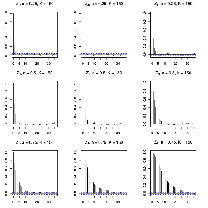
We use Algorithms 2 and 3 find the moral graph. Recall that the moral graph is defined from the nonzero entries in as in Algorithm 4. We then follow Algorithms 5 and 6 to estimate any remaining parameters. The tuning parameters for Algorithms 2 and 3 are chosen by CV as described in Section S.2. This means only choosing . We denote the estimated parameter by . We use 250 simulations to compute the performance of our methodology.
We also test the performance of the PC algorithm when we impose the restrictions provided by Lasso and CLIME. The elements of which are equal to zero represent those edges which we exclude from the skeleton. These restrictions can be embedded in the PC algorithm using the appropriate “fixedGaps” command, which guarantees that will be no edge between nodes j and i if the element of in position is equal to zero. We obtain improved compute time performance of the PC algorithm in this case. This is particularly relevant in the high dimensional case. Imposing the restriction has however nontrivial implications for the PC algorithm, as an edge is deleted without a test so that no variable is included in the separation set. We refer to Algorithm 1 and 2 in Kalisch and Bühlmann (2007) for the details. In general, imposing the restrictions might ensure that we obtain a DAG rather than a CPDAG. It may also be advisable to use a tuning parameter smaller than the one suggested by CV. This is because the PC algorithm can only delete edges, but not add them back. To verify if this is the case, we also report results for and . We find no general evidence in favour of this claim.
We compare our results with two benchmarks. One does not account for sparsity and is essentially equivalent to choosing in the estimation. The second does not account for time series dependence, and carries out the PC algorithm directly on the observed data. We shall refer to these benchmarks as and , respectively. The case should produce sensible results in the low-dimensional case. On the other hand, given that the simulated data are Gaussian, the case should be appropriate when the time series dependence is low.
All approaches are compared on their performance to estimate the contemporaneous causal structure. To achieve this, we report the average structural Hamming distance (SHD) of the estimated causal graph to the true (Acid and de Campos, 2003, Tsamardinos et al., 2006). The SHD between two partially directed acyclic graphs counts how many edge types do not coincide. For instance, estimating a non-edge instead of a directed edge contributes an error of one to the overall distance. We remark that the PC algorithm estimates the Markov equivalence class of a given graph, i.e., the related CPDAG, and some causal structure, as common cause and causal chain, shares the same class, i.e., the same CPDAG, (e.g., for the v-structure the Markov class coincides with the related DAG). Therefore, as the true causal structure in SHD analysis we consider the (block) equivalence class attained by the PC algorithm, with a very high significance level, , to obtain a deterministic estimate performed on the theoretical correlation matrix of each cluster.
Tables S.1 and S.2 display the average SHD and standard errors computed over 250 simulations for all approaches. For the sake of conciseness we only report results for the v-structure for the persistency parameter and the number of clusters 333The complete results are available upon request.. Our approach produces estimators with superior finite sample performance, relatively to the benchmarks, regardless of the considered causal structures. While not reported here, we note that for both the causal chain and common cause, the performance of the PC algorithm deteriorates when we impose the a priori restrictions from the zeros of even if we undersmooth.
The discrepancy among the contemporaneous causal structure is also investigated by computing the number of nonzero elements of . Indeed, we recall that nonzero elements of correspond to possible edges between variables of the corresponding row and column. We also compute the number of false positive and negative between the estimated and true of nonzero elements444We say that an element of is a false positive, if it is estimated as nonzero element while it is zero. Vice versa, it is a false negative, if it is estimated as zero element while it is different from zero.. Tables S.3 and S.4 summarize the results for the high and low dimensional case, respectively. We only report the results for the v-structure, as we can draw similar conclusions for the other causal structures.
| Lasso | |||||||||
| NR | NR | NR | |||||||
| 1000 | 0.25 | 9.208 | 9.212 | 58.032 | 58.160 | 66.080 | 71.616 | 40.424 | 45.628 |
| (0.28) | (0.28) | (0.48) | (0.48) | (0.49) | (0.52) | (0.39) | (0.57) | ||
| 0.75 | 1.960 | 95.888 | 4.464 | 4.488 | 29.596 | 29.556 | 131.060 | 225.212 | |
| (0.14) | (0.2) | (0.2) | (0.2) | (0.35) | (0.34) | (0.93) | (0.48) | ||
| 5000 | 0.25 | 3.124 | 3.124 | 44.700 | 44.776 | 31.092 | 32.504 | 22.144 | 144.944 |
| (0.16) | (0.16) | (0.43) | (0.43) | (0.37) | (0.38) | (0.29) | (0.29) | ||
| 0.75 | 0 | 99.904 | 2.496 | 2.496 | 2.780 | 2.780 | 51.696 | 230.704 | |
| (0) | (0.03) | (0.17) | (0.17) | (0.17) | (0.17) | (0.47) | (0.62) | ||
| CLIME | |||||||||
| NR | NR | NR | |||||||
| 1000 | 0.25 | 27.700 | 27.740 | 53.496 | 53.604 | 78.984 | 83.340 | - | |
| (0.51) | (0.51) | (0.47) | (0.47) | (0.51) | (0.51) | - | |||
| 0.75 | 100.012 | 100.012 | 56.776 | 105.104 | 12.880 | 96.220 | - | ||
| (0.01) | (0.01) | (0.53) | (0.19) | (0.33) | (0.32) | - | |||
| 5000 | 0.25 | 2.488 | 2.488 | 41.744 | 41.892 | 39.896 | 41.104 | - | |
| (0.15) | (0.15) | (0.45) | (0.45) | (0.37) | (0.38) | - | |||
| 0.75 | 119.440 | 138.064 | 3.192 | 4.392 | 6.348 | 6.348 | - | ||
| (0.5) | (0.18) | (0.19) | (0.21) | (0.23) | (0.23) | - | |||
| Lasso | |||||||||
| NR | NR | NR | |||||||
| 1000 | 0.25 | 0.184 | 0.184 | 0.16 | 0.172 | 0.156 | 0.16 | 0.16 | 2.756 |
| (0.04) | (0.04) | (0.04) | (0.04) | (0.04) | (0.04) | (0.04) | (0.16) | ||
| 0.75 | 0.144 | 5.64 | 0.184 | 0.184 | 0.244 | 0.244 | 0.372 | 9.156 | |
| (0.04) | (0.06) | (0.05) | (0.05) | (0.05) | (0.05) | (0.06) | (0.04) | ||
| 5000 | 0.25 | 0.18 | 0.18 | 0.272 | 0.272 | 0.244 | 0.256 | 0.224 | 8.632 |
| (0.05) | (0.05) | (0.05) | (0.05) | (0.05) | (0.05) | (0.05) | (0.07) | ||
| 0.75 | 0 | 6 | 0.144 | 0.144 | 0.136 | 0.136 | 0.332 | 8.712 | |
| (0) | (0) | (0.04) | (0.04) | (0.04) | (0.04) | (0.05) | (0.05) | ||
| CLIME | |||||||||
| NR | NR | NR | |||||||
| 1000 | 0.25 | 0.256 | 0.256 | 0.184 | 0.188 | 0.16 | 0.152 | - | |
| (0.05) | (0.05) | (0.04) | (0.04) | (0.04) | (0.04) | - | |||
| 0.75 | 6.016 | 6.016 | 4.776 | 6.592 | 0.196 | 5.244 | - | ||
| (0.01) | (0.01) | (0.12) | (0.05) | (0.05) | (0.08) | - | |||
| 5000 | 0.25 | 0.18 | 0.18 | 0.264 | 0.264 | 0.256 | 0.26 | - | |
| (0.05) | (0.05) | (0.05) | (0.05) | (0.05) | (0.05) | - | |||
| 0.75 | 0.084 | 5.028 | 0.184 | 0.192 | 0.264 | 0.28 | - | ||
| (0.03) | (0.09) | (0.05) | (0.05) | (0.05) | (0.05) | - | |||
| Lasso | |||||||||||||
| TP+FP | FP | FN | TP+FP | FP | FN | TP+FP | FP | FN | TP+FP | FP | FN | ||
| 1000 | 0.25 | 313.44 | 13.44 | 0 | 2197.832 | 1897.8 | 0 | 9711.5 | 9411.5 | 0 | 22350 | 22050 | 0 |
| (0.33) | (0.33) | (0) | (4.24) | (4.24) | (0) | (7.83) | (7.83) | (0) | (0) | (0) | (0) | ||
| 0.75 | 210.344 | 4.72 | 94.376 | 549.104 | 249.1 | 0.024 | 2109.6 | 1809.6 | 0 | 22350 | 22050 | 0 | |
| (0.3) | (0.19) | (0.23) | (1.31) | (1.31) | (0.01) | (3.35) | (3.35) | (0) | (0) | (0) | (0) | ||
| 5000 | 0.25 | 302.52 | 2.52 | 0 | 1472.928 | 1172.9 | 0 | 8488.2 | 8188.2 | 0 | 22350 | 22050 | 0 |
| (0.15) | (0.15) | (0) | (3.14) | (3.14) | (0) | (7.81) | (7.81) | (0) | (0) | (0) | (0) | ||
| 0.75 | 200.096 | 0 | 99.904 | 300 | 0 | 0 | 343.08 | 43.08 | 0 | 22350 | 22050 | 0 | |
| (0.03) | (0) | (0.03) | (0) | (0) | (0) | (0.59) | (0.59) | (0) | (0) | (0) | (0) | ||
| CLIME | |||||||||||||
| TP+FP | FP | FN | TP+FP | FP | FN | TP+FP | FP | FN | |||||
| 1000 | 0.25 | 300.928 | 0.928 | 0 | 1189.848 | 889.8 | 0 | 6638.7 | 6338.7 | 0 | - | - | - |
| (0.09) | (0.09) | (0) | (3.18) | (3.18) | (0) | (6.96) | (6.96) | (0) | - | - | - | ||
| 0.75 | 106.144 | 0 | 193.856 | 187.472 | 13.248 | 125.7 | 1024 | 807.4 | 83.424 | - | - | - | |
| (0.21) | (0) | (0.21) | (0.63) | (0.36) | (0.5) | (2.75) | (2.71) | (0.33) | - | - | - | ||
| 5000 | 0.25 | 300.56 | 0.56 | 0 | 760.752 | 460.7 | 0 | 4570.88 | 4270.8 | 0 | - | - | - |
| (0.06) | (0.06) | (0) | (2.45) | (2.45) | (0) | (6.59) | (6.59) | (0) | - | - | - | ||
| 0.75 | 235.48 | 0.032 | 64.552 | 318.344 | 19.544 | 1.2 | 764.216 | 464.2 | 0 | - | - | - | |
| (0.5) | (0.02) | (0.5) | (0.4) | (0.39) | (0.1) | (2) | (2) | (0) | - | - | - | ||
| Lasso | |||||||||||||
| TP+FP | FP | FN | TP+FP | FP | FN | TP+FP | FP | FN | TP+FP | FP | FN | ||
| 1000 | 0.25 | 22.968 | 4.968 | 0 | 41.584 | 23.584 | 0 | 57.48 | 39.48 | 0 | 72 | 54 | 0 |
| (0.24) | (0.24) | (0) | (0.41) | (0.41) | (0) | (0.34) | (0.34) | (0) | (0) | (0) | (0) | ||
| 0.75 | 12.504 | 0.016 | 5.512 | 18.456 | 0.456 | 0 | 22.168 | 4.168 | 0 | 72 | 54 | 0 | |
| (0.06) | (0.01) | (0.06) | (0.06) | (0.06) | (0) | (0.16) | (0.16) | (0) | (0) | (0) | (0) | ||
| 5000 | 0.25 | 18 | 0 | 0 | 20.808 | 2.808 | 0 | 38.04 | 20.04 | 0 | 72 | 54 | 0 |
| (0) | (0) | (0) | (0.16) | (0.16) | (0) | (0.35) | (0.35) | (0) | (0) | (0) | (0) | ||
| 0.75 | 12 | 0 | 6 | 18 | 0 | 0 | 18.12 | 0.12 | 0 | 72 | 54 | 0 | |
| (0) | (0) | (0) | (0) | (0) | (0) | (0.03) | (0.03) | (0) | (0) | (0) | (0) | ||
| CLIME | |||||||||||||
| TP+FP | FP | FN | TP+FP | FP | FN | TP+FP | FP | FN | |||||
| 1000 | 0.25 | 19.256 | 1.256 | 0 | 30.792 | 12.792 | 0 | 46.072 | 28.072 | 0 | - | - | - |
| (0.11) | (0.11) | (0) | (0.34) | (0.34) | (0) | (0.37) | (0.37) | (0) | - | - | - | ||
| 0.75 | 6.16 | 0 | 11.84 | 9.456 | 0.016 | 8.56 | 14.104 | 1.152 | 5.048 | - | - | - | |
| (0.05) | (0) | (0.05) | (0.12) | (0.01) | (0.11) | (0.12) | (0.1) | (0.08) | - | - | - | ||
| 5000 | 0.25 | 18 | 0 | 0 | 19.056 | 1.056 | 0 | 28.872 | 10.872 | 0 | - | - | - |
| (0) | (0) | (0) | (0.1) | (0.1) | (0) | (0.29) | (0.29) | (0) | - | - | - | ||
| 0.75 | 13.096 | 0.04 | 4.944 | 19.088 | 1.096 | 0.008 | 22.408 | 4.424 | 0.016 | - | - | - | |
| (0.09) | (0.02) | (0.09) | (0.09) | (0.09) | (0.01) | (0.17) | (0.17) | (0.01) | - | - | - | ||
Finally, in Tables S.5 and S.6, we assess the finite sample performance of the estimators of and and analyse their asymptotic properties stated in Theorem 7. We compute the average distance from the true matrices, where the distance is measured in terms of the operator’s norm: the largest singular value. These statistics are compared only to the case .
| Lasso | CLIME | |||||||
|---|---|---|---|---|---|---|---|---|
| 1000 | 0.25 | 0.567 | 1.25 | 2.354 | 0.684 | 1.082 | 2.639 | 314.10 |
| (0.003) | (0.003) | (0.006) | (0.006) | (0.003) | (0.012) | (3.106) | ||
| 0.75 | 4.265 | 1.093 | 1.095 | 0.798 | 3.290 | 3.812 | >1000 | |
| (0.048) | (0.006) | (0.003) | (0.016) | (0.083) | (0.054) | (-) | ||
| 5000 | 0.25 | 0.131 | 0.369 | 0.722 | 0.297 | 0.307 | 0.644 | 24.610 |
| (0.001) | (0.001) | (0.001) | (0.005) | (0.001) | (0.001) | (0.061) | ||
| 0.75 | 3.604 | 0.925 | 0.135 | 3.555 | 1.404 | 0.250 | >1000 | |
| (0.016) | (0.001) | (0.001) | (0.101) | (0.048) | (0.001) | (-) | ||
| Lasso | CLIME | |||||||
| 1000 | 0.25 | 0.258 | 1.394 | 1.803 | 0.292 | 1.143 | 2.531 | 0.916 |
| (0.002) | (0.007) | (0.009) | (0.002) | (0.007) | (0.019) | (0.001) | ||
| 0.75 | 0.430 | 0.119 | 0.228 | 0.118 | 0.335 | 0.616 | 0.331 | |
| (0.006) | (0.001) | (0.0014) | (0.003) | (0.007) | (0.006) | (0.003) | ||
| 5000 | 0.25 | 0.081 | 0.367 | 0.511 | 0.076 | 0.316 | 0.582 | 0.395 |
| (0.001) | (0.001) | (0.002) | (0.002) | (0.001) | (0.002) | (0.001) | ||
| 0.75 | 0.314 | 0.039 | 0.043 | 0.390 | 0.184 | 0.052 | 0.109 | |
| (0.001) | (0.001) | (0.001) | (0.002) | (0.010) | (0.001) | (0.001) | ||
| Lasso | CLIME | |||||||
|---|---|---|---|---|---|---|---|---|
| 1000 | 0.25 | 0.243 | 0.331 | 0.345 | 0.307 | 0.311 | 0.343 | 12.716 |
| (0.004) | (0.004) | (0.004) | (0.007) | (0.004) | (0.004) | (0.122) | ||
| 0.75 | 2.835 | 0.845 | 0.182 | 0.673 | 1.774 | 2.186 | >1000 | |
| (0.039) | (0.005) | (0.004) | (0.012) | (0.079) | (0.055) | (-) | ||
| 5000 | 0.25 | 0.079 | 0.097 | 0.140 | 0.078 | 0.091 | 0.129 | 10.495 |
| (0.001) | (0.002) | (0.002) | (0.002) | (0.002) | (0.002) | (0.049) | ||
| 0.75 | 2.963 | 0.853 | 0.050 | 3.143 | 0.840 | 0.100 | >1000 | |
| (0.017) | (0.002) | (0.001) | (0.027) | (0.010) | (0.009) | (-) | ||
| Lasso | CLIME | |||||||
| 1000 | 0.25 | 0.149 | 0.176 | 0.169 | 0.125 | 0.185 | 0.179 | 0.158 |
| (0.004) | (0.003) | (0.002) | (0.004) | (0.003) | (0.002) | (0.002) | ||
| 0.75 | 0.262 | 0.051 | 0.057 | 0.086 | 0.180 | 0.397 | 0.062 | |
| (0.005) | (0.001) | (0.001) | (0.002) | (0.007) | (0.008) | (0.001) | ||
| 5000 | 0.25 | 0.035 | 0.060 | 0.082 | 0.035 | 0.050 | 0.084 | 0.072 |
| (0.001) | (0.001) | (0.001) | (0.001) | (0.001) | (0.001) | (0.001) | ||
| 0.75 | 0.257 | 0.022 | 0.022 | 0.415 | 0.024 | 0.028 | 0.027 | |
| (0.002) | (0.001) | (0.001) | (0.004) | (0.001) | (0.002) | (0.001) | ||
References
- [1] Bhatia, R. (1996) Matrix Analysis. New York: Springer.
- [2] Burman, P. and D. Nolan (1992) Data Dependent Estimation of Prediction Functions. Journal of Time Series Analysis 13, 189-207.
- [3] Cai, T., W. Liu and X. Luo (2011) A Constrained Minimization Approach to Sparse Precision Matrix Estimation. Journal of the American Statistical Association 106, 594-607.
- [4] Han, F. and W.B. Wu (2019) Probability Inequalities for High Dimensional Time Series Under a Triangular Array Framework. https://arxiv.org/abs/1907.06577v1.
- [5] Joe, H. (1997) Multivariate Models and Dependence Models. London: Chapman & Hall.
- [6] Kalisch, M. and P. Bühlmann (2007) Estimating High-Dimensional Directed Acyclic Graphs with the PC-Algorithm. Journal of Machine Learning Research 8, 613-636.
- [7] Lauritzen, S. L. (1996) Graphical Models. Oxford: Oxford University Press.
- [8] Le, T.-M. and P.-S. Zhong (2021) High-Dimensional Precision Matrix Estimation with a Known Graphical Structure. Stat 11, e424.
- [9] Liu, H., F. Han, M. Yuan, J. Lafferty and L. Wasserman (2012) High Dimensional Semiparametric Gaussian Copula Graphical Models. The Annals of Statistics 40, 2293-2326.
- [10] Loh, P.-L. and M. J. Wainwright (2012) High-Dimensional Regression With Noisy and Missing Data: Provable Guarantees With Nonconvexity. The Annals of Statistics 40, 1637-1664.
- [11] Meinshausen, N. and P. Bühlmann (2006) High-Dimensional Graphs and Variable Selection with the Lasso. The Annals of Statistics 34, 1436-1462.
- [12] Rüschendorf, L. and V. de Valk (1993) On Regression Representation of Stochastic Processes. Stochastic Processes and their Applications 46, 183-198.
- [13] van de Geer, S. A. and P. Bühlmann (2009) On the conditions used to prove oracle results for the lasso. Electronic Journal of Statistics 3, 1360-1392.
- [14] van der Vaart, A. and J.A. Wellner (2000) Weak Convergence and Empirical Process Theory. New York: Springer.