Corrected Hill Function in Stochastic Gene Regulatory Networks

Abstract

Describing reaction rates in stochastic bio-circuits is commonly done by directly introducing the deterministically deduced Hill function into the master equation. However, when fluctuations in enzymatic reaction rates are not neglectable, the Hill function must be derived, considering all the involved stochastic reactions. In this work, we derived the stochastic version of the Hill function from the master equation of the complete set of reactions that, in the macroscopic limit, lead to the Hill function reaction rate. We performed a series expansion around the average values of the concentrations, which allowed us to find corrections for the deterministic Hill function. This process allowed us to quantify the fluctuations of enzymatic reactions. We found that the underlying variability in propensity rates of gene regulatory networks has an important non-linear effect that reduces the intrinsic fluctuations of the mRNA and protein concentrations.

Keywords: Hill function, stochastic system, fluctuations, genetic networks, stationary distribution.

1 Introduction

The study of genetic regulatory networks has increased in recent years, owing to their potential applications in novel disease treatments. Understanding the dynamics and functional relationships among the components of the regulatory networks of some genetic diseases [2, 3] can provide insights into their causes and lead to new treatments. These systems are complex, and contain several components. However, the transcription factors and protein concentrations involved in network dynamics are generally low. The effect of fluctuations around average concentrations can propagate between many components or even play a functional role. Thus, a deterministic description of the evolution of the network concentrations is an approximation. Many models have been proposed in the context of stochastic processes [4, 5] using the master equation. Most of these approaches employ a deterministically derived Hill function to represent certain chemical rates, implying that they are approximations of a complete reaction network. This problem was previously addressed by [6]; however, its consequences and the problem itself have yet to be exhaustively studied. However, some developments have been made in this regard [6, 7, 8].

The formalism of multivariable birth-dead processes [9] is typically employed to describe reaction kinetics. However, in addition to the simple reactions, the master equation is difficult to solve analytically. Furthermore, as the reaction network becomes more complex, the numerical solutions become more computationally intensive.

This lack of practicality in finding a solution to the master equation results in a linear noise approximation that leads to the Fokker-Planck equation, which is the standard framework for making inferences about stochastic systems [9, 10]. The Fokker-Planck equation is useful for a wide range of situations and systems. In [15] a similar approximation was considered, although only second-order reactions were also considered. Although we work with a model of any order, it is necessary for the system to be sufficiently large. The results obtained contain a corrective term. In [15] a similar approximation was considered, although they only worked with second-order reactions, whereas we worked with a model of any order; only for reactions of order greater than 2, it is necessary that the size of the system is large enough for the approximation to the second order to be sufficient. The results obtained contain a corrective term. However, before the approximation is made, it is possible to take advantage of the separation between fast and slow reactions in some scenarios.

In this work, we obtained general expressions for the master equation based on the assumption that there are fast and slow reactions in the chemical network, where the fast reactions have already reached their equilibrium distributions. This procedure provides a more accurate description than inserting a Hill function to describe an enzymatic response, as is commonly performed.

The master equation for the slow reactions was then used to obtain the evolution of the average reactant concentrations as a series of expansions of relative fluctuations. This calculation was necessary because the mean concentrations were generally associated with deterministic reaction kinetics equations. Thus, this procedure allows us to correct the deterministic dynamics of small systems where the effect of intrinsic fluctuations cannot be neglected.

This method was illustrated using three examples. First, we found the corrections of the Hill function due to reactant concentration fluctuations in small systems using a Toggle Switch. With this gained experience, an expression for the master equation of a general gene regulatory network was provided and used to analyze a repressilator and an activator-repressor clock.

The proposed methodology helps find a more accurate description of complex reaction kinetics for small systems than deterministic models. It is also an improvement over the simplistic application of the Hill function for describing the reaction rates of enzymatic reactions in a stochastic manner. Additionally, the resulting ordinary differential equations are significantly more computationally efficient than the expensive computer simulations of the Gillespie algorithm [11, 12]. This approximation will allow for simulation and thus, a better understanding of more complex systems and the role of fluctuations in chemical networks. In particular, it is possible to analyze the effect of intrinsic noise in complex gene regulatory networks and the potential emergent properties from the inherent noise in these types of systems.

The remainder of this paper is structured as follows.

In Section 2, we briefly describe the multivariable life and death processes and propose a useful variation of the method presented in [13] for determining the stationary distribution of this type of system. The methodology is used in the following sections because fast reactions are assumed to have reached their stationary distribution.

Section 3 describes a method for obtaining deterministic equations from a stochastic model, particularly for multivariable life and death systems. In addition, we find the corresponding fluctuation-dissipation theorem, which allows us to quantify the fluctuations of the variables throughout the time evolution.

Section 4 briefly explains how the Hill function was obtained from a stochastic process. In particular, we first analyzed the toggle switch to explain in more detail how the Hill function was obtained. To achieve this, we assumed fast and slow reactions. Using a similar procedure, we calculated the Hill function with corrections owing to the stochastic effects.

Section 5 presents a generic gene regulation network. This study was divided into two broad categories. First, we present a general network with one transcription factor, and then the study is broadened to consider many transcription factors.

In Section 6, we review the results and provide concluding remarks.

2 Chemical master equation

In deterministic models, the law of mass action is used to build a set of differential equations that describe the concentration dynamics of the species for some network of chemical processes. However, this approach may not always be the most suitable for small systems, because the relative fluctuations become significant. The mass action law can be generalized in the stochastic realm as a multivariable birth-dead-like process [9]. In this section, the methodology and notation used to describe the birth-dead process are reviewed.

We consider $N$ species $\mathcal{S}_{j}$ ($j$ $\in$ $1,2,..N$), and $M$ reactions $\mathcal{R}_{i}$ ($i$ $\in$ $1,2,..M$) through which these species are transformed, that is,

$$\mathcal{R}_{i}:\sum_{j=1}^{N}\alpha_{ij}\mathcal{S}_{j}\stackbin[k_{i}^{-}]{k_{i}^{+}}{\rightleftarrows}\sum_{j=1}^{N}\beta_{ij}\mathcal{S}_{j}.$$ (1)

The coefficients $\alpha_{ij}$ and $\beta_{ij}$ are positive integers known as stoichiometric coefficients. The stoichiometric matrix is defined as

$$\Gamma_{ji}=\beta_{ij}-\alpha_{ij}.$$ (2)

Through collisions (or interactions) of the species, they may be transformed; therefore, the transformation rates are proportional to the collision probability. The propensity rates can be expressed as follows [9]

$${t_{i}^{+}(\mathbf{S})} =k_{i}^{+}\prod_{l}\frac{S_{l}!}{\Omega^{\alpha_{il}}(S_{l}-\alpha_{il})!}, {t_{i}^{-}(\mathbf{S})}=k_{i}^{-}\prod_{l}\frac{S_{l}!}{\Omega^{\beta_{il}}(S_{l}-\beta_{il})!}.$$ (3)

( index $i$ labels the reaction that occurs $\mathcal{R}_{i}$). Where $S_{l}$ is the number of molecules of species $\mathcal{S}_{l}$ and $\mathbf{S}=(S_{1},S_{2},...,S_{N})$ is the state vector. These ratios are the transition probabilities between different states of the system. $\Omega$ is closely related to the system size. According to (1), we labeled reactions that go from left to right as $t^{+}_{i}(\mathbf{S})$ and when they move in the opposite direction as $t^{-}_{i}(\mathbf{S})$. With all of the above elements, we can write the master equation of the system, which describes the dynamic evolution of the probability distribution of the states of the system. The master equation can then be expressed as

$$\partial_{t}P(\mathbf{S},t)=\Omega\sum_{i} \left(t_{i}^{-}(\mathbf{S}+\Gamma_{i})P(\mathbf{S}+\Gamma_{i},t)-t_{i}^{+}(\mathbf{S})P(\mathbf{S},t)\right.$$

$$+\left.t_{i}^{+}(\mathbf{S}-\Gamma_{i})P(\mathbf{S}-\Gamma_{i},t)-t_{i}^{-}(\mathbf{S})P(\mathbf{S},t)\right).$$ (4)

Where $\Gamma_{i}$ denotes the $i$ column of the stoichiometric matrix. The sum is made over all the reactions of the system. This equation is also known as the master chemical equation and is the stochastic version of the law of mass action. Let $\mathcal{S}=\{\mathcal{S}_{i}\}$ be the set of species, $\mathcal{R}=\{\mathcal{R}_{i}\}$ be the set of reactions, $\mathbf{t}=\{t_{i}^{+},t_{i}^{-}\}$ be the set of reaction rates of the system, and $\{\mathcal{S},\mathcal{R},\mathbf{t}\}$ be called the chemical reaction network (CRN).

2.1 Calculation of the stationary distribution

We will assume that the fast reactions reach their stationary state well before the slow reactions. Thus, when describing the dynamics of slow reactions, we assume that fast reactions are already stationary. In this section, we develop the methodology used to calculate the stationary distribution of the master equation.

The stationary distribution is the solution of (4) when its LHS is set to zero

$$0= \sum_{i}\left(t_{i}^{-}(\mathbf{S}+\Gamma_{i})P(\mathbf{S}+\Gamma_{i},t)-t_{i}^{+}(\mathbf{S})P(\mathbf{S},t)\right.$$

$$+\left.t_{i}^{+}(\mathbf{S}-\Gamma_{i})P(\mathbf{S}-\Gamma_{i},t)-t_{i}^{-}(\mathbf{S})P(\mathbf{S},t)\right).$$ (5)

Several proposals have been made to solve (5) [9, 13]. We follow a procedure similar to [13] with a slight variation. As shown in [13], a stationary distribution of a CRN that is at least weakly reversible and has zero deficiency can be expressed in the form

$$P(\textbf{S})_{S}=\prod_{i}P_{i}(S_{i}).$$ (6)

Where $P_{i}(S_{i})$ represents the probability of finding $S_{i}$ molecules of species $i$. Then we proceed as follows,

1. We define

   $$\nu^{+}_{i}(\mathbf{S}) =t_{i}^{+}(\mathbf{S})P(\mathbf{S}), \nu^{-}_{i}(\mathbf{S}) =t_{i}^{-}(\mathbf{S})P(\mathbf{S}).$$ (7)

2. By complex balance [13], the stationary distribution obey the following system of equations

   $$\sum_{j}\Gamma_{ij}(\nu^{+}_{j}(\mathbf{S})\theta(\Gamma_{ij})+\nu^{-}_{j}(\mathbf{S})\theta(-\Gamma_{ij}))=\sum_{j}\Gamma_{ij}(\nu^{+}_{j}(\mathbf{S}-\Gamma_{j})\theta(-\Gamma_{ij})+\nu^{-}_{j}(\mathbf{S}+\Gamma_{j})\theta(\Gamma_{ij})).$$ (8)

   where $\Gamma_{ij}$ is the stoichiometric matrix, and $\theta(x)$ is the Heaviside step function.

3. There might be equations that are linearly dependent on others, meaning that, depending on the particular form of $\Gamma_{ij}$ we could have more equations than unknowns in the system (8). In this case, we can transform the similarity to represent $\Gamma_{ij}$ in its reduced echelon form $\Gamma_{ij}^{\prime}$. If there are linearly dependent columns, this means that there are conserved quantities. Thus the linear independent system of equation is

   $$\sum_{j}\Gamma_{ij}^{\prime}(\nu^{+}_{j}(\mathbf{S})\theta(\Gamma_{ij}^{\prime})+\nu^{-}_{j}(\mathbf{S})\theta(-\Gamma_{ij}^{\prime}))=\sum_{j}\Gamma_{ij}^{\prime}(\nu^{+}_{j}(\mathbf{S}-\Gamma_{j}^{\prime})\theta(-\Gamma_{ij}^{\prime})+\nu^{-}_{j}(\mathbf{S}+\Gamma_{j}^{\prime})\theta(\Gamma_{ij}^{\prime})).$$ (9)

4. Substituting (6) in (9) and taking the average over all variables except a single specie $S_{i}$ we obtain an equation for $P_{i}(S_{i})$

   $$\sum_{j}\Gamma_{ij}^{\prime}(\braket{t^{+}_{j}(\mathbf{S})}_{l\neq i}P_{i}(S_{i})\theta(\Gamma_{ij}^{\prime})+\braket{t^{-}_{j}(\mathbf{S})}_{l\neq i}P_{i}(S_{i})\theta(-\Gamma_{ij}^{\prime}))=$$

   $$\sum_{j}\Gamma_{ij}^{\prime}\braket{t^{+}_{j}(\mathbf{S})}_{l\neq i}P_{i}(S_{i}-\Gamma_{ij})\theta(-\Gamma_{ij}^{\prime})+\braket{t^{+}_{j}(\mathbf{S})}_{l\neq i}P_{i}(S_{i}+\Gamma_{ij})\theta(\Gamma_{ij}^{\prime})).$$ (10)

   This procedure can be repeated for the remaining species of the system. After solving for each species it is possible to find the stationary distribution around a stationary state

   $$P(\mathbf{S})=\prod_{i}M\frac{c_{i}^{S_{i}}}{S_{i}!}\prod_{l}\delta_{\sum_{i}\gamma_{li}S_{i}-N_{l},0}.$$ (11)

   Here the coefficient $M$ is a normalization constant, $c_{i}$ characterise the mean concentration of specie $i$, $\gamma_{li}$ are the null vectors of the stoichiometric matrix, $N_{l,0}$ are the conserved quantities of the system. We introduce the Kronecker delta to consider that there could be some dependent variables in $\mathbf{S}$ labeled by index $l$.

3 Deterministic approximation and the dissipation fluctuation theorem

Deterministic models of chemical reactions typically describe the dynamics of average concentrations of the species. Thus, the deterministic model associated with a master equation is obtained by calculating the average number of molecules divided by the system size $\frac{\braket{S_{j}}}{\Omega}$ using the master equation (4). Thus, the temporal evolution of the concentration of the species $\mathcal{S}_{j}$ is

$$\frac{\partial}{\partial{t}}\left(\frac{\braket{S_{j}}}{\Omega}\right)=\sum_{i}\Gamma_{ij}\braket{t_{i}^{+}(\mathbf{S})-t_{i}^{-}(\mathbf{S})},$$ (12)

where the bracket notation $\braket{f(\mathbf{S})}=\sum_{\mathbf{S}}{f(\mathbf{S})}P(\mathbf{S},t)$ is the average of all the variables. In the following, we denote the average concentrations with the lower letters $s_{j}=\frac{\braket{S_{j}}}{\Omega}$.

To obtain an approximate expression of the RHS in (12), we use the Taylor expansion of a function around the average of its argument, that is,

$$\braket{f(\mathbf{X})}\approx \left\langle f(\braket{\mathbf{X}})+\sum_{i}(X_{i}-\braket{X_{i}})\left[\frac{\partial f(\mathbf{X})}{\partial X_{i}}\right]_{\mathbf{X}=\braket{\mathbf{X}}}+\sum_{i}\sum_{j}\frac{(X_{i}-\braket{X_{i}})(X_{j}-\braket{X_{j}})}{2}\left[\frac{\partial^{2}f(\mathbf{X})}{\partial X_{i}\partial X_{j}}\right]_{\mathbf{X}=\braket{\mathbf{X}}}\right\rangle$$

$$= f(\braket{\mathbf{X}})+\sum_{i}\sum_{j}\frac{\sigma^{2}(X_{i},X_{j})}{2}\left[\frac{\partial^{2}f(\mathbf{X})}{\partial X_{i}\partial X_{j}}\right]_{\mathbf{X}=\braket{\mathbf{X}}},$$ (13)

for large enough $\Omega$, where $\braket{\mathbf{X}}=(\braket{X_{1}},\braket{X_{2}},...,\braket{X_{N}})$ and

$$\sigma^{2}(X_{i},X_{j})=\left\langle(X_{i}-\braket{X_{i}})(X_{j}-\braket{X_{j}})\right\rangle=\braket{X_{i}X_{j}}-\braket{X_{i}}\braket{X_{j}}.$$ (14)

as been defined.

Thus, we can express the averages rates $\braket{t^{\pm}(\mathbf{S})}$ using the previous 2nd order expansion to obtain

$$\braket{t_{i}^{+}(\mathbf{S})}\approx k_{i}^{+}\left(\prod_{j}s_{j}^{\alpha_{ij}}+\sum_{l_{1}}\sum_{l_{2}}\frac{\sigma^{2}(s_{l_{1}},s_{l_{2}})}{2}\left[\frac{\partial^{2}}{\partial s_{l_{1}}\partial s_{l_{2}}}\left(\prod_{j}s_{j}^{\alpha_{ij}}\right)\right]\right),$$

$$\braket{t_{i}^{-}(\mathbf{S})}\approx k_{i}^{-}\left(\prod_{j}s_{j}^{\beta_{ij}}+\sum_{l_{1}}\sum_{l_{2}}\frac{\sigma^{2}(s_{l_{1}},s_{l_{2}})}{2}\left[\frac{\partial^{2}}{\partial s_{l_{1}}\partial s_{l_{2}}}\left(\prod_{j}s_{j}^{\beta_{ij}}\right)\right]\right),$$ (15)

where we have also made use of Stirling’s approximation to eliminate factorials, i.e.

$$t_{i}^{+}(\braket{\mathbf{S}})=k_{i}^{+}\prod_{j}\frac{\braket{S_{j}}!}{\Omega^{\alpha_{ij}}(\braket{S_{j}}-\alpha_{ij})!}\approx k_{i}^{+}\prod_{j}\left(\braket{\frac{S_{j}}{\Omega}}\right)^{\alpha_{ij}}=k_{i}^{+}\prod_{j}s_{j}^{\alpha_{ij}}\equiv R_{i}^{D+}({\mathbf{s}}),$$

$$t_{i}^{-}(\braket{\mathbf{S}})=k_{i}^{-}\prod_{j}\frac{\braket{S_{j}}!}{\Omega^{\beta_{ij}}(\braket{S_{j}}-\beta_{ij})!}\approx k_{i}^{-}\prod_{j}\left(\braket{\frac{S_{j}}{\Omega}}\right)^{\beta_{ij}}=k_{i}^{-}\prod_{j}s_{j}^{\beta_{ij}}\equiv R_{i}^{D-}({\mathbf{s}}).$$ (16)

Finally, if we denote $k_{i}^{+}\prod_{j}s_{j}^{\alpha_{ij}}=R_{i}^{D+}({\mathbf{s}})$ and $k_{i}^{-}\prod_{j}s_{j}^{\beta_{ij}}=R_{i}^{D-}({\mathbf{s}})$ as the deterministic reaction rates when $\Omega\rightarrow\infty$ we write the evolution of concentration $s_{j}$ as

$$\frac{ds_{j}}{d{t}}= \sum_{i}\Gamma_{ji}\left(R_{i}^{D+}(\mathbf{s})-R_{i}^{D-}(\mathbf{s})+\sum_{j_{1}}\sum_{j_{2}}\frac{\sigma^{2}(s_{j_{1}},s_{j_{2}})}{2}\frac{\partial^{2}}{\partial{s_{j_{1}}}\partial{s_{j_{2}}}}(R_{i}^{D+}(\mathbf{s})-R_{i}^{D-}(\mathbf{s}))\right).$$ (17)

This equation provides the first stochastic correction to the deterministic evolution of the reaction kinetics. However, it is not yet a closed system of equations; we also need the evolution of covariance $\sigma^{2}(s_{j_{1}},s_{j_{2}})$ to solve it.

As before, we use the master equation to find the evolution of $\braket{X_{i}X_{j}}$, and then we use the expansion (13) on the reactions rates $R_{i^{\prime}s}$ to obtain

$$\frac{\partial}{\partial{t}}\sigma^{2}(s_{l_{1}},s_{l_{2}}) =\sum_{i}\left(\Gamma_{l_{1}i}\Gamma_{l_{2}i}\frac{(R_{i}^{D+}(\mathbf{s})+R_{i}^{D-}(\mathbf{s}))}{\Omega}\right.$$

$$+\sum_{j_{1}}\left({\sigma^{2}(s_{l_{1}},s_{j_{1}})}\Gamma_{l_{2}i}\frac{\partial}{\partial{s_{j_{1}}}}+{\sigma^{2}(s_{j_{1}},s_{l_{2}})}\Gamma_{l_{1}i}\frac{\partial}{\partial{s_{j_{1}}}}\right){(R_{i}^{D+}(\mathbf{s})-R_{i}^{D-}(\mathbf{s}))}$$

$$+\left.\sum_{j_{1}}\sum_{j_{2}}\{\sigma^{2}(s_{j_{1}},s_{j_{2}})\frac{\Gamma_{l_{1}i}\Gamma_{l_{2}i}}{2\Omega}\frac{\partial^{2}}{\partial{s_{j_{1}}}\partial{s_{j_{2}}}}(R_{i}^{D+}(\mathbf{s})+R_{i}^{D-}(\mathbf{s}))\right),$$ (18)

It is worth noting that, in contrast to the common Linear Noise Approximation, the cross-reaction terms from equations (17) and (18) give us a closed system, and thus the exact expressions for second-order reactions [14].

As the intrinsic fluctuations of the species concentrations are given by

$$\eta^{2}_{i}=\frac{\braket{\xi_{i}^{2}}}{\Omega^{2}}=\frac{\sigma^{2}(X_{i},X_{i})}{\Omega^{2}},$$ (19)

where $\xi_{i}^{2}=(X_{i}-\braket{X_{i}})^{2}$. Subsequently, the system of differential equations formed by (17) and (18) describes the mean dynamics of the system and quantifies its intrinsic fluctuations. Thus, instead of solving the entire master equation, it is possible to solve the more simple equations (17) and (18). In the following sections, we use the method to describe representative stochastic systems and demonstrate its advantages.

4 Hill function and its fluctuations-induced correction

The Hill function is widely used in systems in which an enzymatic reaction occurs, or, in our case, to capture the transcription rate of factors affecting mRNA synthesis. Generally, transcription factors act as activators or suppressors. In the case of an activating factor, the following Hill function is usually used,

$$H=\frac{\hat{e}^{n}}{K^{n}+\hat{e}^{n}}.$$ (20)

Here, $\hat{e}$ are the concentrations of the factors and $n$ is known as the Hill coefficient. Figure 1 shows how the Hill function behaves for an activator with different values of $n$. In the case of a repressor, the Hill function used is of the form $D=K^{n}/(K^{n}+\hat{e})$.

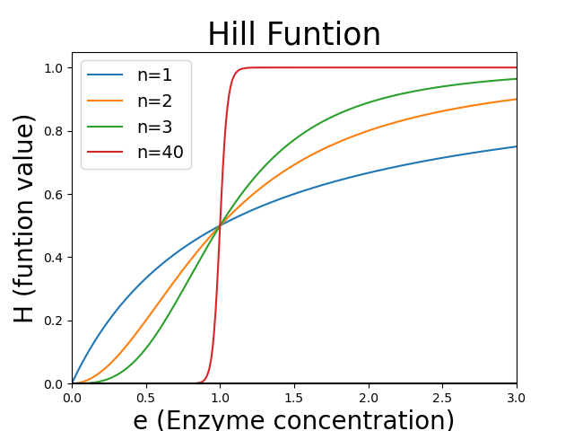
Figure 1: Deterministic Hill function, with $K=1$.

Hill functions are derived by analyzing the deterministic dynamics of enzymatic reactions, and their use is widely extended, even in stochastic descriptions. However, its direct use as a transcription rate in the master equation of a stochastic system is just an approximation [6]. In this section, we derive the exact transcription rate due to stationary enzymatic reactions by setting up the master equation of the entire reaction network of the system. This procedure allows us to find corrections of the Hill function to consider the intrinsic fluctuations of enzymatic reactions. First, we will analyze the Toggle switch as a particular case, and then derive a general expression for the corrections.

4.1 Toggle switch

Now, we will analyze the Toggle switch genetic regulatory network to show a common approach used in the literature. Then we will pose the master equation of the complete reaction network corresponding to the system. A systematic treatment of the master equation will allow us to show that the commonly used Hill function is a first approximation and that corrections can be made.

The standard approach to describe the Toggle switch is to use the following chemical network

$$\emptyset \xrightarrow{\alpha D_{d}(R_{2})}R_{1}, \emptyset\xrightarrow{\alpha D_{d}(R_{1})}R_{2},$$

$$R_{1} \xrightarrow{\beta}\emptyset, R_{2}\xrightarrow{\beta}\emptyset.$$ (21)

where $D_{d}$ is the deterministic derived Hill function $D_{d}$, defined by

$$D_{d}(x)=\frac{(\frac{x}{K_{R}})^{n}}{1+(\frac{x}{K_{R}})^{n}}.$$ (22)

The corresponding master equation of the system is given by [16, 17]

$$\frac{d}{dt}P(r_{1},r_{2},t) =\alpha\Omega D_{d}(\frac{r_{2}}{\Omega})P(r_{1}-1,r_{2},t)-\beta{r_{1}}P(r_{1},r_{2},t)$$

$$+ \beta({r_{1}+1})P(r_{1}+1,r_{2},t)-\alpha\Omega D_{d}(\frac{r_{2}}{\Omega})P(r_{1},r_{2},t)$$

$$+\alpha\Omega D_{d}(\frac{r_{1}}{\Omega})P(r_{1},r_{2}-1,t)-\beta{r_{2}}P(r_{1},r_{2},t)$$

$$+ \beta({r_{2}+1})P(r_{1},r_{2}+1,t)-\alpha\Omega D_{d}(\frac{r_{1}}{\Omega})P(r_{1},r_{2},t).$$ (23)

In the previous description of the Toggle switch, the Hill Function in the master equation (23) is introduced because of the assumption that the enzymatic reaction leading to the production of $R_{1}$ and $R_{2}$ implicitly involves an enzyme at a fixed concentration [6]. For a more accurate description, the intrinsic fluctuations of the available active molecules should be considered, even if the enzyme concentration is stationary. We included the binding reactions between $R_{1}$ and $R_{2}$ to the corresponding enzyme to account for these enzymatic fluctuations. The reaction network of the Toggle Switch then becomes.

$$P_{R_{1}} +nR_{2}\stackbin[k_{-}]{k_{+}}{\rightleftarrows}P_{R_{1}}^{*}, P_{R_{2}}+nR_{1}\stackbin[k_{-}]{k_{+}}{\rightleftarrows}P_{R_{2}}^{*},$$

$$P_{R_{1}} \xrightarrow{\alpha^{\prime}}R_{1}, P_{R_{2}}\xrightarrow{\alpha^{\prime}}R_{2},$$

$$R_{1} \xrightarrow{\beta}\emptyset, R_{2}\xrightarrow{\beta}\emptyset.$$ (24)

We will denote $r_{1}$ as the number of molecules of the chemical species $R_{1}$ and $p_{1}$ for the active polymerase $P_{R_{1}}$, and $p_{1}^{*}$ for the deactivated polymerase $P_{R_{1}}^{*}$. Similarly, $r_{2}$ represents the number of molecules of species $R_{2}$ and $p_{2}$, $p_{2}^{*}$ is the corresponding active and inactivated polymerase $P_{R_{2}}$, $P_{R_{2}}^{*}$. To clarify the first reactions, we must remember that in the Toggle Switch, $R_{1}$ inhibits $R_{2}$ and vice versa. Thus, if $n$ molecules of $R_{2}$ bind to the promoter region of $P_{R_{1}}$, they deactivate it. The same process is true for bidding $R_{1}$ and $P_{R_{2}}$.

The reactions that occur in the promoter are fast (the first line of reactions in (24)); thus, we consider that they have already reached an equilibrium. On the other hand, protein synthesis is a slow process. Therefore, we separate the master equation into a stationary part corresponding to fast reactions and a dynamic part describing slow reactions [7].

$$\dot{P}(r_{1}, r_{2},p_{1},p_{2},p_{1}^{*},p_{2}^{*},t)=\alpha^{\prime}({p_{2}+1})P(r_{1}-1,r_{2},p_{1},p_{2},p_{1}^{*},p_{2}^{*},t)-\alpha^{\prime}{p_{1}}P(r_{1},r_{2},p_{1},p_{2},p_{1}^{*},p_{2}^{*},t)$$

$$+\alpha^{\prime}({p_{1}+1})P(r_{1},r_{2}-1,p_{1},p_{2},p_{1}^{*},p_{2}^{*},t)-\alpha^{\prime}{p_{2}}P(r_{1},r_{2},p_{1},p_{2},p_{1}^{*},p_{2}^{*},t)$$

$$+\beta({r_{1}+1})P(r_{1}+1,r_{2},p_{1},p_{2},p_{1}^{*},p_{2}^{*},t)-\beta{r_{1}}P(r_{1},r_{2},p_{1},p_{2},p_{1}^{*},p_{2}^{*},t)$$

$$+\beta({r_{2}+1})P(r_{1},r_{2}+1,p_{1},p_{2},p_{1}^{*},p_{2}^{*},t)-\beta{r_{2}}P(r_{1},r_{2},p_{1},p_{2},p_{1}^{*},p_{2}^{*},t),$$

$$0= \Omega^{n}k_{-}(p_{1}^{*}+1)P(r_{1},r_{2}-n,p_{1}-1,p_{2},p_{1}^{*}+1,p_{2}^{*})-k_{+}p_{1}\frac{r_{2}!}{(r_{2}-n)!}P(r_{1},r_{2},p_{1},p_{2},p_{1}^{*},p_{2}^{*})$$

$$+k_{+}(p_{1}+1)\frac{(r_{2}+n)!}{r_{2}!}P(r_{1},r_{2}+n,p_{1}+1,p_{2},p_{1}^{*},p_{2}^{*}-1)-\Omega^{n}k_{-}p_{1}^{*}P(r_{1},r_{2},p_{1},p_{2},p_{1}^{*},p_{2}^{*})$$

$$+\Omega^{n}k_{-}(p_{2}^{*}+1)P(r_{1}-n,r_{2},p_{1},p_{2}-1,p_{1}^{*},p_{2}^{*}+1)-k_{+}p_{2}\frac{r_{1}!}{(r_{1}-n)!}P(r_{1},r_{2},p_{1},p_{2},p_{1}^{*},p_{2}^{*})$$

$$+k_{+}(p_{2}+1)\frac{(r_{1}+n)!}{r_{1}!}P(r_{1}+n,r_{2},p_{1},p_{2}+1,p_{1}^{*},p_{2}^{*}-1)-\Omega^{n}k_{-}p_{2}^{*}P(r_{1},r_{2},p_{1},p_{2},p_{1}^{*},p_{2}^{*}),$$ (25)

in these equations, we denote $r_{1}$ as the number of elements of the chemical species $R_{1}$ and $p_{1}$ to the active polymerase, $p_{1}^{*}$ to the deactivated polymerase, and we denote the remaining variables similarly.

We now take the average over the stationary variables $p_{1}$ and $p_{2}$ on the equation (25) obtaining and effective master equation for only the variables $r_{1}$ and $r_{2}$,

$$\dot{P}(r_{1},r_{2},t) =\alpha^{\prime}\braket{p_{2}}_{s}P(r_{1}-1,r_{2},t)-\alpha^{\prime}\braket{p_{1}}_{s}P(r_{1},r_{2},t)$$

$$+\alpha^{\prime}\braket{p_{1}}_{s}P(r_{1},r_{2}-1,t)-\alpha^{\prime}\braket{p_{2}}_{s}P(r_{1},r_{2},t)$$

$$+\beta({r_{1}+1})P(r_{1}+1,r_{2},t)-\beta{r_{1}}P(r_{1},r_{2},t)$$

$$+\beta({r_{2}+1})P(r_{1},r_{2}+1,t)-\beta{r_{2}}P(r_{1},r_{2},t).$$ (26)

On the other hand, the solution of the stationary distribution (25) can be explicitly obtained (see Section 2), and thus we can calculate $\alpha^{\prime}\braket{p_{2}}_{s}=\alpha\Omega D_{1}({r_{1}},{\Omega})$ and $\alpha^{\prime}\braket{p_{1}}_{s}=\alpha\Omega D_{1}({r_{2}},{\Omega})$ where

$$D_{1}(x,\Omega)=\frac{K^{n}}{K^{n}+\frac{\braket{\frac{x!}{(x-n)!}}_{x}}{\Omega^{n}}}\qquad\textrm{with}\qquad K\equiv\frac{k_{+}}{k_{-}}.$$ (27)

Substituting this result we obtain a closed master equation describing $r_{1}$ and $r_{2}$

$$\dot{P}(r_{1},r_{2},t) =\alpha\Omega D_{1}({r_{1}},{\Omega})P(r_{1},r_{2}-1,t)-\alpha\Omega D_{1}({r_{2}},{\Omega})P(r_{1},r_{2},t)$$

$$+\alpha\Omega D_{1}({r_{2}},{\Omega})P(r_{1}-1,r_{2},t)-\alpha\Omega D_{1}({r_{1}},{\Omega})P(r_{1},r_{2},t)$$

$$+\beta(r_{1}+1)P(r_{1}+1,r_{2},t)-\beta{r_{1}}P(r_{1},r_{2},t)$$

$$+\beta(r_{2}+1)P(r_{1},r_{2}+1,t)-\beta{r_{2}}P(r_{1},r_{2},t).$$

Furthermore, using the fact that

$$\braket{f(\mathbf{X})}\approx f(\braket{\mathbf{X}})+\sum_{i}\sum_{j}\frac{(\sigma^{2}(X_{i},X_{j})}{2}\left[\frac{\partial^{2}f(\mathbf{X})}{\partial X_{i}\partial X_{j}}\right]_{\mathbf{X}=\braket{\mathbf{X}}},$$ (28)

we approximate

$$D_{1}(x,\Omega)=\frac{K^{n}}{K^{n}+\frac{\braket{\frac{x!}{(x-n)!}}}{\Omega^{n}}}\approx\frac{K^{n}}{K^{n}+\frac{\braket{x}^{n}+\frac{n}{2}(n-1)\sigma^{2}(x,x)\braket{x}^{n-2}}{\Omega^{n}}}.$$ (29)

where $\sigma^{2}(x,x)$ is the variance of $x$ around its average $\braket{x}$. This is the first correction to the Hill function due to fluctuations in species concentrations. With this example, it is clear that introducing the Hill function directly into the master equation does not consider fluctuations ($\sigma^{2}(x,x)=0$). Furthermore, to make the first corrections to the Hill function, the following transformation is necessary.

$$\hat{x}^{n}\rightarrow\hat{x}^{n}+\frac{n}{2}(n-1)\sigma^{2}(\hat{x},\hat{x})\hat{x}^{n-2}.$$ (30)

In the following, we refer to (29) as the Hill function with stochastic corrections.

5 Stochastic genetic regulation networks

As we are interested in describing the stochastic version of a gene regulatory network, we will briefly explain how a transcription/translation module (TTM) works. When several of these modules are connected, they form a gene regulatory network; more strictly speaking, one of the proteins produced by one of these modules acts as a transcription factor for other TTMs.

Figure 2 is a simplified schematic view of a TTM, where a $X$ protein is the input of the module acting as a transcription factor, the transcription process occurs in which the mRNA is synthesized, and translation occurs where some new $Y$ proteins are synthesized from the mRNA.

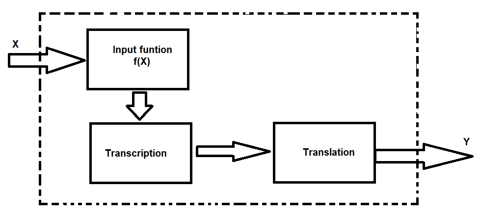
Figure 2: Transcription/translation module.

Hill function is typically used to express the production rate of a protein in terms of its activator. More specifically, it helps to describe the number of active promoters as a function of transcription factor concentration.

5.1 Stochastic genetic regulatory network

The most simple description of a MTT can be described with the following reactions

$$x \stackbin{H}{\rightarrow}\text{mRNA}\stackbin{k_{2}}{\rightarrow}y$$

mRNA $$\stackbin{\gamma_{m}}{\rightarrow}0,$$

y $$\stackbin{\gamma_{p}}{\rightarrow}0.$$ (31)

The first reaction indicates that mRNA is synthesized by transcription factor $x$ with a reaction rate proportional to the Hill function. Subsequently, it is synthesized into a protein $y$, and the last two reactions indicate that the mRNA and protein are degraded and diluted. In the reaction rates, $H$ is a Hill function, which can be an activator or a suppressor depending on the system. Hill function would be a repressor if the protein suppressed gene activation; otherwise, it would be an activator.

In a more general sense, many transcription factors can act on the same gene giving effectively a more complex Hill function of the form

$$H_{i}(\mathbf{p})=\frac{\sum_{j}\lvert A_{ij}\lvert\left(\frac{p_{j}}{\Omega K_{j}}\right)^{n_{ij}*A_{ij}}}{1+\sum_{j}\lvert A_{ij}\lvert\left(\frac{p_{j}}{\Omega K_{j}}\right)^{n_{ij}*A_{ij}}},$$ (32)

where $A_{ij}$ is the connections matrix with elements $A_{il}=1$ if $l$ activates $i$, and $A_{ij}=-1$ if $j$ repress $i$, otherwise $A_{ij}=0$. The numbers $n_{ij}$ are called to the Hill coefficients, and $K_{j}$ are the Michelson-Menten constants.

The general expression of the master equation describing a gene regulatory network is given by (31),

$$\frac{\partial P(\mathbf{m},\mathbf{p},t)}{\partial t}= \sum_{i}\left({\Omega k_{1i}}\left(H_{i}(\mathbf{p},{\Omega})P(\mathbf{m},\mathbf{p},m_{i}-1,t)-H_{i}(\mathbf{p},{\Omega})P(\mathbf{m},\mathbf{p},t)\right)\right.$$

$$+\frac{m_{i}+1}{\tau_{1i}}P(\mathbf{m},\mathbf{p},m_{i}+1,t)-\frac{m_{i}}{\tau_{1i}}P(\mathbf{m},\mathbf{p},t)$$

$$+k_{2i}{m_{i}}P(\mathbf{m},\mathbf{p},p_{i}-1,t)-k_{2i}{m_{i}}P(\mathbf{m},\mathbf{p},t)$$

$$\left.+\frac{p_{i}+1}{\tau_{2i}}P(\mathbf{m},\mathbf{p},p_{i}+1,t)-\frac{p_{i}}{\tau_{2i}}P(\mathbf{m},\mathbf{p},t)\right),$$ (33)

where $\tau_{1i}=\frac{1}{\gamma_{m_{i}}}$ and $\tau_{2i}=\frac{1}{\gamma_{p_{i}}}$ are mRNA and protein degradation times, respectively. Index $i$ labels each MTT, and there is a sum over all network modules.

In expression (33), it is customary to use operators to supply the Hill function [19, 20] or directly use the deterministic Hill function [16]; however, we have the option of using a generalized Hill function with stochastic corrections.

Making the LHS of eq. 33, the fluctuations in the steady state can been exactly calculated to be

$$\eta_{m_{i}}^{2} =\frac{\braket{m_{i}}}{\Omega^{2}}, \eta_{p_{i}}^{2} =\frac{\braket{p_{i}}}{\Omega^{2}}.$$ (34)

This particular expression, which is proportional to the first moment of the variables, originates from the fact that a Poisson distribution purely describes the stationary distribution. In this case $\braket{m_{i}}$ and $\braket{p_{i}}$ are the number of molecules, but in terms of concentrations, the fluctuations are proportional to the inverse of the system size in contrast to its square as in (34).

To illustrate the proposed analysis and its advantages, we will present two examples.

5.2 Repressilator

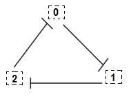
Figure 3: Represilator. Each node represents a TTM.

Figure 3 shows a graphical representation of the repressilator. This simple but important system has been experimentally developed [18]. With the help of figure 3 we build its connection matrix $A$

$$A_{ij}=\begin{pmatrix}0&0&-1\\ -1&0&0\\ 0&-1&0\end{pmatrix},$$ (35)

the first row of matrix $A$ indicates that a protein synthesized in module 2 acts as a suppressor in module 0 and similarly in the other modules. The corresponding master equation is

$$\frac{\partial P(\mathbf{m},\mathbf{p},t)}{\partial t}= \sum_{i=1}^{3}\left(\left(k_{1}^{-}\Omega\left(H_{i}(\mathbf{p},{\Omega})P(\mathbf{m},\mathbf{p},m_{i}-1,t)-H_{i}(\mathbf{p},{\Omega})P(\mathbf{m},\mathbf{p},t)\right)\right)\right.$$

$$+\frac{m_{i}+1}{\tau_{1i}}P(\mathbf{m},\mathbf{p},m_{i}+1,t)-\frac{m_{i}}{\tau_{1i}}P(\mathbf{m},\mathbf{p},t)$$

$$+k_{2i}{m_{i}}P(\mathbf{m},\mathbf{p},p_{i}-1,t)-k_{2i}{m_{i}}P(\mathbf{m},\mathbf{p},t)$$

$$\left.+\frac{p_{i}+1}{\tau_{2i}}P(\mathbf{m},\mathbf{p},p_{i}+1,t)-\frac{p_{i}}{\tau_{2i}}P(\mathbf{m},\mathbf{p},t)\right).$$ (36)

The Hill functions $H_{i}(\mathbf{p},{\Omega})$ are repressors.

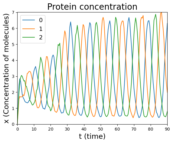
Figure 4: Repressilator. Stochastic simulation using the Gillespie algorithm and deterministic Hill function. In the first figure, the concentration of mRNA is shown, and in the second figure, the concentration of proteins is shown. The following parameters are used: $n=2$, $\Omega=200$, $\tau_{1i}=\tau_{2i}=1$, $k_{1i}=k_{2i}=10$.

We can now analyze the system using three different approaches. First, we simulated the system dynamics using the Gillespie algorithm, assuming deterministic Hill functions for reaction rates. Second, the description can be performed by approximating the deterministic dynamics in conjunction with TFD using the deterministically derived Hill function. Finally, we can describe the system dynamics using the deterministic approximation and dynamics of the fluctuations but using the Hill function with stochastic correction, an expression similar to (29).

A Gillespie simulation of the system is shown in figures 4. In this case, we used the deterministic Hill function, and the size of the system is 200 (as in the Elowitz experiment [18]). We plotted the protein and mRNA concentrations. This is simply a realization of a stochastic system; thus, the amplitudes of the oscillations are not uniform.

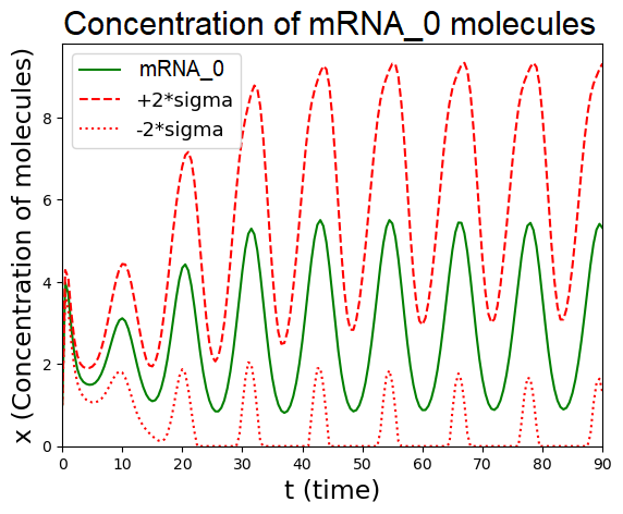
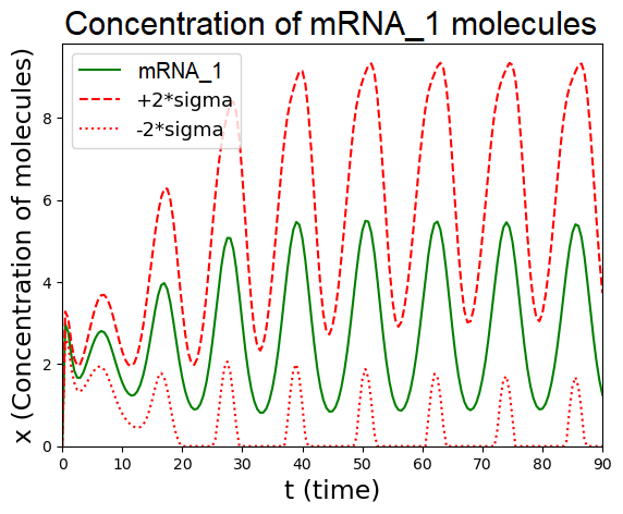
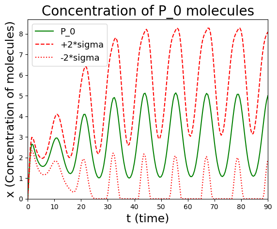
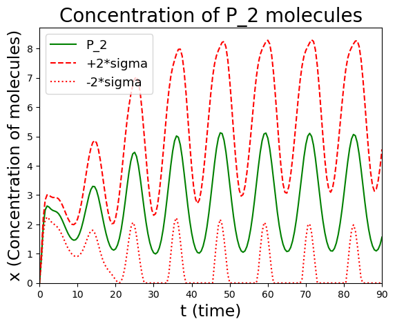
Figure 5: Repressilator. Dynamics of deterministic concentrations and fluctuations from stochastic simulations with an assembly of $10000$ simulations. In the upper figures, the dynamics of the mRNAs are observed in the lower ones of the proteins. The green lines represent the deterministic concentrations, and the red dotted lines represent the bands where fluctuations are found. The following parameters were used: $Arm_{1}(0)=Arm_{2}(0)=r_{0}(0)=r_{1}(0)=r_{2}(0)=0$, $Arm_{1}(0)=\Omega$, n=2, $\Omega=200$, $\tau_{1i}=\tau_{2i}=1$, $k_{1i}=k_{2i}=10$.

By creating an ensemble of simulations, the average or deterministic dynamics as well as the fluctuations were obtained (see Fig. 5). In Fig. 5 it is plotted the concentration of the mRNA and the region of the fluctuations.

In figure 7 (a), we plot the analytically obtained deterministic dynamics and deduce the region of fluctuations using FDT [16].

Finally, using the Hill function with stochastic correction, we obtain Figure 7. b. The most notable result is that the size of the fluctuations is considerably reduced compared to Figures 5 and 7. a. At first sight, this might be counterintuitive, but it shows that the stochastic effect in the reaction rates might have no linear effects on gene regulatory networks that make them robust with respect to intrinsic noise.

We can compare the prediction of fluctuations in the steady state of the approximations with the exact result. In fig. 6, we plotted the characteristic size of the fluctuations using the Hill function and the Hill function with stochastic corrections, and it is compared with the exact calculation. It is observed that the corrected Hill function provides a much better description of the stochastic system.

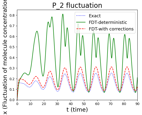
Figure 6: Fluctuations. We plotted the fluctuations obtained using the deterministic approach and FDT, first with the deterministic Hill function (green line) and then with the Hill function with stochastic corrections. Finally, we compared these results with those obtained analytically in steady state.

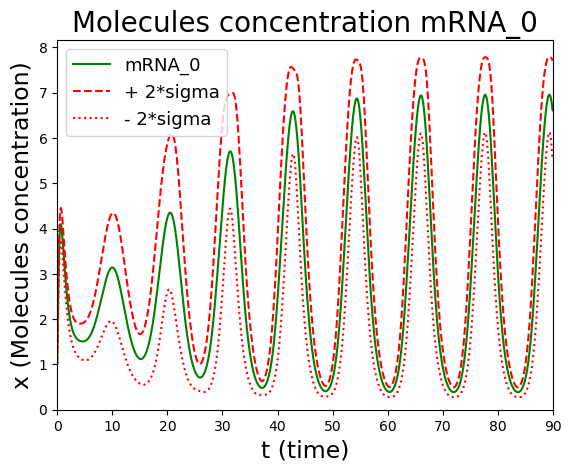
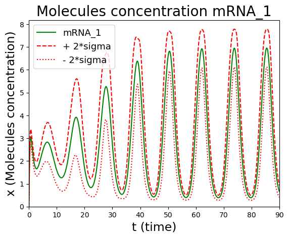
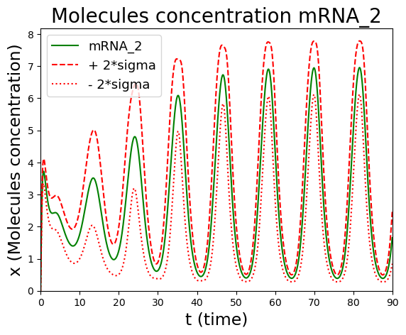
(a) Deterministic Hill function.

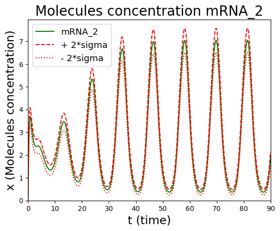
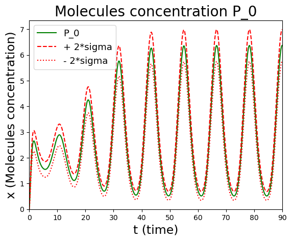
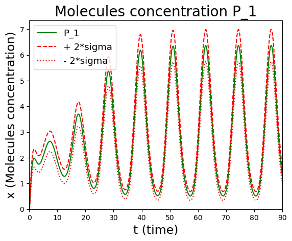
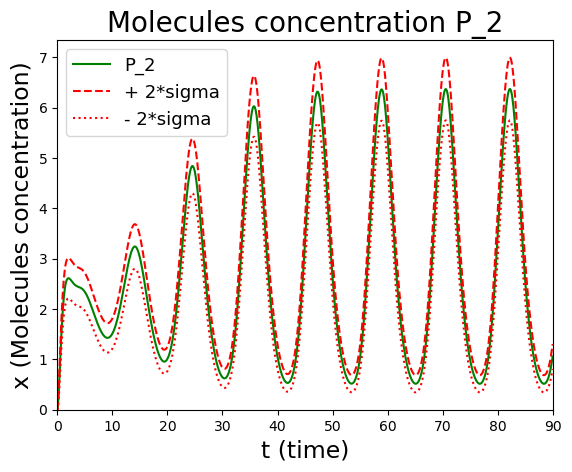
(b) Hill function with stochastic corrections.

Figure 7: Represilador. The dynamics and fluctuations of the system were modeled using a deterministic approach and FDT, as shown in Figure (a). A deterministic Hill function was used. In (b), the Hill function with stochastic corrections is used. For both (a) and (b), the figures at the top show the dynamics of the mRNAs, whereas those at the bottom show the dynamics of the proteins. The green lines represent the deterministic concentrations, and the red dotted lines represent the bands where fluctuations are found. The following parameters have been used: $Arm_{2}(0)=r_{1}(0)=r_{2}(0)=0$, $Arm_{1}(0)=1$, n=2, $\Omega=200$, $\tau_{2i}=\tau_{3i}=1$, $k_{2i}=k_{3i}=10$.

5.3 Activator-repressor clock

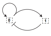
Figure 8: Activador-represor clock. Each node represents a TTM.

A genetic network in which several transcription factors participate is the activator-repressor clock. First, we analyze the system with the Gillespie algorithm using the deterministic Hill function, then we use the FDT with the deterministic Hill function, and finally, we analyze it using stochastic corrections to the Hill function. Figure 8 presents a graphical representation of the model. The matrix of connections of the system is

$$A_{ij}=\begin{pmatrix}1&-1\\ 1&0\end{pmatrix}.$$ (37)

In module 0, the protein synthesized by module 1 acts as a suppressor, whereas the protein synthesized by module 0 acts as an activator. The protein synthesized by module 0 acts as an activator of module 1. We assume that $k_{1i}=k_{1}$, also $n_{11}=n_{12}=n_{21}=2$ and $n_{22}=0$, $\beta_{11}=\beta{21}=1$, $\beta_{11}=0.0004$ so the master equation is

$$\frac{\partial P(\mathbf{m},\mathbf{p},t)}{\partial t} =\sum_{i=1}^{2}\left(k_{1i}\Omega\left(H_{g}^{i}(\mathbf{p},{\Omega})P(\mathbf{m},\mathbf{p},m_{i}-1,t)-H_{g}^{i}(\mathbf{p},{\Omega})P(\mathbf{m},\mathbf{p},t)\right)\right.$$

$$+\frac{m_{i}+1}{\tau_{2i}}P(\mathbf{m},\mathbf{p},m_{i}+1,t)-\frac{m_{i}}{\tau_{2i}}P(\mathbf{m},\mathbf{p},t)$$

$$+k_{3i}{m_{i}}P(\mathbf{m},\mathbf{p},p_{i}-1,t)-k_{3i}{m_{i}}P(\mathbf{m},\mathbf{p},t)$$

$$+\left.\frac{p_{i}+1}{\tau_{3i}}P(\mathbf{m},\mathbf{p},p_{i}+1,t)-\frac{p_{i}}{\tau_{3i}}P(\mathbf{m},\mathbf{p},t)\right).$$ (38)

Where the Hill functions take the form

$$H_{g}^{1}({p_{1}},p_{2},{\Omega})= \frac{\beta_{1}\left(\frac{p_{1}}{K_{1}^{\prime}\Omega}\right)^{{n_{11}}}+\alpha_{0}}{1+\left(\frac{p_{1}}{K_{1}^{\prime}\Omega}\right)^{{n_{11}}}+\left(\frac{p_{2}}{K_{2}\Omega}\right)^{n_{12}}}, H_{g}^{2}({p_{1}},{\Omega})= \frac{\beta_{2}\left(\frac{p_{1}}{K_{1}\Omega}\right)^{{n_{21}}}}{1+\left(\frac{p_{1}}{K_{1}\Omega}\right)^{{n_{21}}}}.$$ (39)

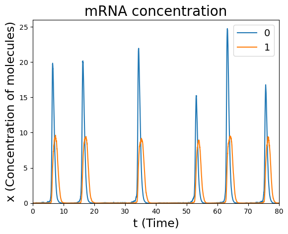
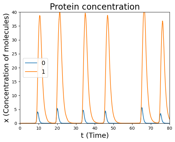
Figure 9: Activator-repressor clock. Stochastic simulation using the Gillespie algorithm and the deterministic Hill function. In the first figure, the concentration of mRNA is shown, and in the second figure, the concentration of proteins is shown. The following parameters have been used: $n_{11}=n_{12}=n_{21}=$2, $\Omega=180$, $k_{11}=250$, $k_{12}=30$, $\alpha_{0}=0.0004$ $\tau_{2i}=\frac{1}{3}$, $\tau_{31}=\frac{1}{3}$, $\tau_{32}=1$, $k_{21}=1$, $k_{21}=3$.

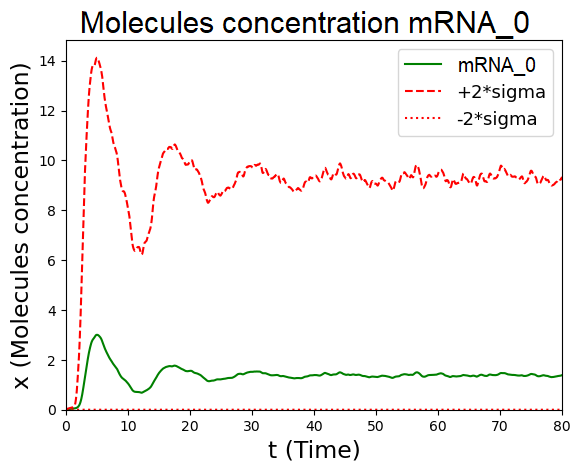
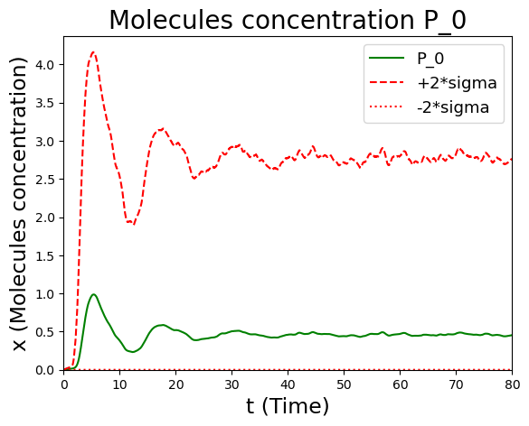
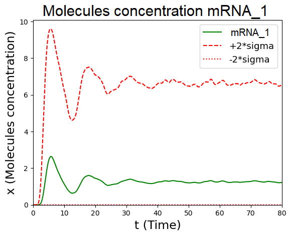
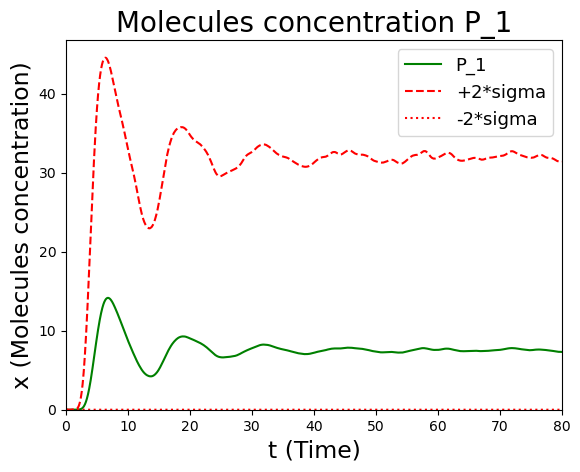
(a) Stochastic simulations.

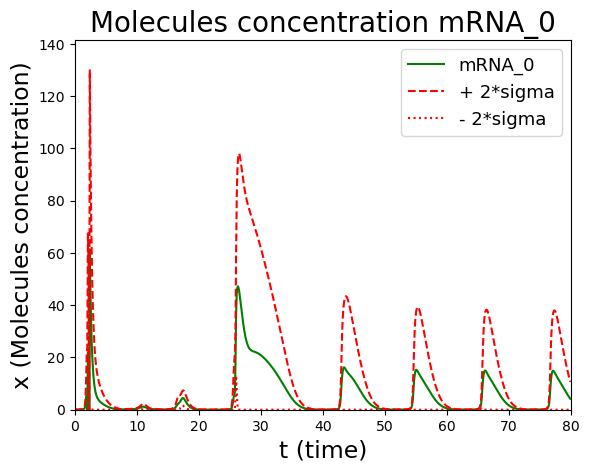
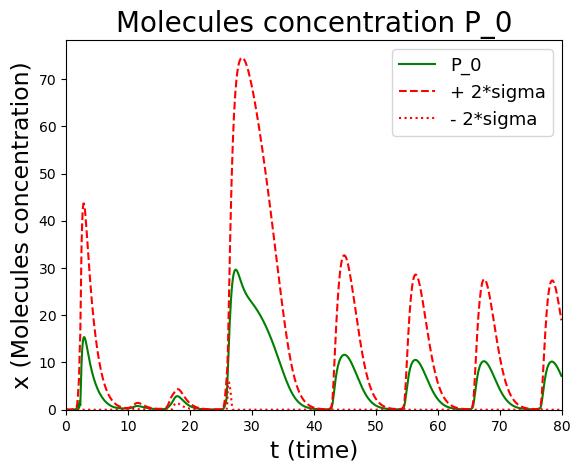
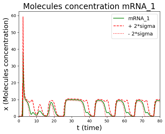
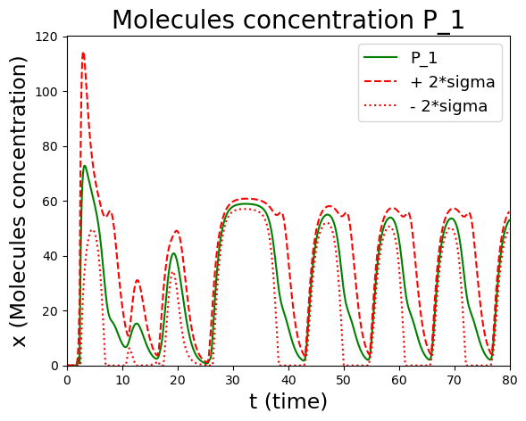
(b) Deterministic Hill function.

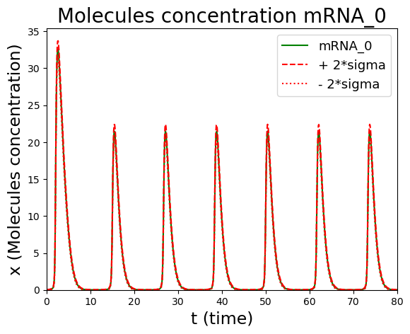
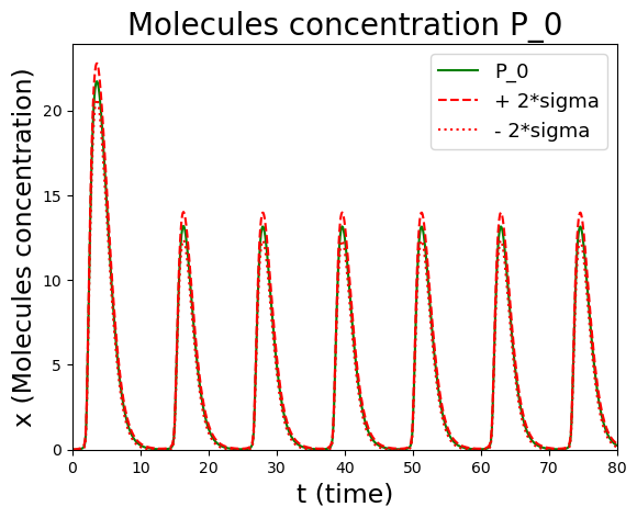
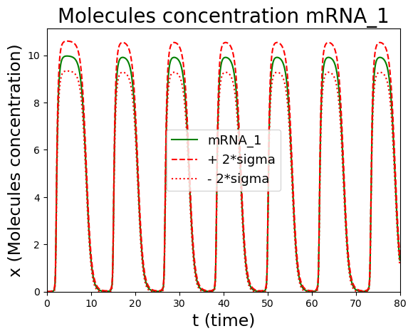
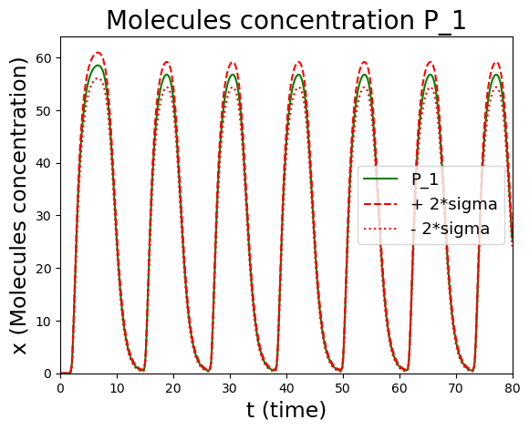
(c) Hill function with stochastic corrections.

Figure 10: Activator-repressor clock. The dynamics and fluctuations of the system were modeled using stochastic simulations with an assembly size$=10000$, as shown in Figure (a), the deterministic approach, and TFD (b). The deterministic Hill function was used. In (c), the Hill function with stochastic corrections is used. The green lines represent the deterministic concentrations, and the red dotted lines represent the bands where fluctuations are found. The following parameters have been used: $n_{11}=n_{12}=n_{21}=$2, $\Omega=180$, $k_{11}=250$, $k_{12}=30$, $\alpha_{0}=0.0004$ $\tau_{2i}=\frac{1}{3}$, $\tau_{31}=\frac{1}{3}$, $\tau_{32}=1$, $k_{21}=1$, $k_{21}=3$.

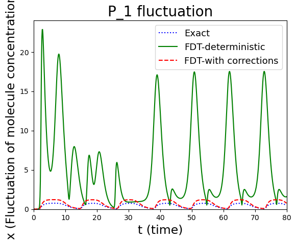
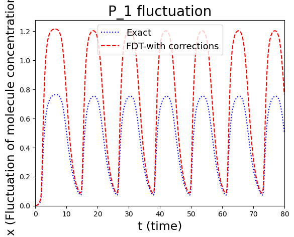
Figure 11: Fluctuations. We plotted the fluctuations obtained in the deterministic approach and TFD, first with the deterministic Hill function (green line) and then with the Hill function with stochastic corrections. Finally, we compared these results with those obtained analytically in the steady state.

By employing the Gillespie algorithm to simulate the system and using the deterministic Hill function, we obtain Figure 9.

By analyzing an ensemble of Gillespie simulations, Figure 10 (a) is obtained. The figure shows the average dynamics and range of fluctuations. It is worth noting that averaging many fluctuating trajectories from the output of the Gillespie simulations makes the average value tend to be stationary in the long run. This occurs even if a single realization is constantly oscillating. This shows that this approach does not help describe the characteristic dynamics of a single system, as it represents the collective behavior of many systems. The deterministic approximation and the fluctuation-dissipation theorem (FDT) [16], using the deterministic Hill function, provide the characteristic size of the fluctuations, as shown in Fig. 10(b). Furthermore, the characteristic dynamics and size of the fluctuations using the corrected Hill functions are shown in Fig. 10(c). Again, we see that the reaction rate fluctuations have feedback effects that compensate for fluctuations in the other variables.

Fluctuations around the steady state are shown in fig. 11 and compared with the exact result.

6 Results and conclusions

The proposed second-order expansion of the reaction rates around the average dynamics of a stochastic system allowed us to describe the mesoscopic dynamics and fluctuations of the system more accurately than the Linear Noise Approximation and the commonly used dissipation fluctuation theorem ([9, 16]). Furthermore, the approach describes the dynamics of the covariances exactly for second-order reactions. This approximation allowed us to obtain a corrected Hill function that considers the change in the effective reaction rate that it describes due to the underlying fluctuations in the enzymatic processes. The corrected Hill function can be introduced straightforwardly to describe gene regulatory networks, where standard Hill functions are typically used. As the corrected Hill function depends on the average and variance of the concentrations, it is not introduced in the master equation but in the deterministic description (mesoscopic dynamics) and characterization of the size of its fluctuations. We used the proposed algorithm to analyse the dynamics and fluctuations in gene regulatory networks and compare the different approximations. Specifically, by examining the size of the fluctuations using the corrected Hill function and the fluctuations obtained by the Gillespie algorithm and the TFD with the traditional Hill function, it was observed that the fluctuations in Hill-type propensity rates, have a feedback effect that reduces the intrinsic fluctuations in the dynamics of the species involved in gene regulatory networks. In particular, this effect was observed in both the repressilator and the activator-repressor clock.

This approach will allow us to study the intrinsic noise effect in more complex and larger network structures, as it is significantly more computationally efficient than the Gillespie algorithm.

Appendix A Stochastic derivation of Hill function

Now, our objective is to derive the Hill function from a stochastic process. If we remember that the derivation or deterministic function relies on the steady state, we will also make a similar choice, although in this case, we will look at the stationary distribution. We use the method presented in Section 2, and the stationary distribution allows us to determine the fluctuations of the system.

We suppose that we have a protein $p$ to which $n$ enzymes $e$ can bind, forming $s=pe_{n}$, we also ask that the enzyme $e$ arrive or go to the system and this can also degrade, so our system is described by the following reversible processes

$$\emptyset \stackbin[\lambda_{-}]{\lambda_{+}}{\rightleftarrows}e, p+ne\stackbin[k_{-}]{k_{+}}{\rightleftarrows}s.$$ (40)

Note that the derivations made in this section are valid only when only two previous reactions are found in the system. As we have already explained, the master equation of a chemical network can be obtained from the formalism developed in section 2 (multivariable life and death processes), for this, we first define our stoichiometric coefficient matrices and the stoichiometric matrix

$$\alpha_{ij} =\begin{pmatrix}0&0&0\\ n&1&0\end{pmatrix}, \beta_{ij} =\begin{pmatrix}1&0&0\\ 0&0&1\end{pmatrix}, \Gamma_{ij} =\begin{pmatrix}1&-n\\ 0&-1\\ 0&1\end{pmatrix},$$ (41)

With the help of these, we calculate the propensity rates and we get

$$t_{1}^{+} =\lambda_{+}, t_{1}^{-}=\lambda_{-}e\frac{1}{\Omega},$$

$$t_{2}^{+} =k_{+}p\frac{e!}{(e-n)!}\frac{1}{\Omega^{n+1}}, t_{2}^{-}=k_{-}s\frac{1}{\Omega}.$$ (42)

(The subscript 1 corresponds to the reaction on the left of (40), while 2 corresponds to the right.) To find the master equation of the system, we substitute all the quantities we have calculated, we finally get our master equation

$$\dot{P}(e,p,s,t) =k_{-}(s+1)P(e-n,p-1,s+1,t)-k_{+}p\frac{e!}{(e-n)!}\frac{1}{\Omega^{n}}P(e,p,s,t)$$

$$+k_{+}(p+1)\frac{(e+n)!}{e!}\frac{1}{\Omega^{n}}P(e+n,p+1,s-1,t)-k_{-}sP(e,p,s,t)$$

$$+\lambda_{+}\Omega P(e-1,p,s,t)-\lambda_{-}eP(e,p,s,t)$$

$$+ \lambda_{-}(e+1)P(e+1,p,s,t)-\lambda_{+}\Omega P(e,p,s,t),$$ (43)

if we consider that our system reaches equilibrium very quickly, then it is enough to look at the stationary distribution so that the previous relationship will be zero, then we need to find the stationary distribution, for this, we use the method that we have presented previously since we have a conserved quantity, the total number of active and inactive proteins is constant, that is $N_{0}=p+s$ (to make contact with the deterministic part it is convenient to define $N_{0}=N_{0d}\Omega$, being $N_{0d}$ the deterministic initial condition), if we substitute the constant we will obtain

$$0 =k_{-}(s+1)P(e-n,s+1)-k_{+}(N_{0}-s)\frac{e!}{(e-n)!}\frac{1}{\Omega^{n}}P(e,s)$$

$$+k_{+}(N_{0}-s+1)\frac{(e+n)!}{e!}\frac{1}{\Omega^{n}}P(e+n,s-1)-k_{-}sP(e,s)$$

$$+\lambda_{+}\Omega P(e-1,s)-\lambda_{-}eP(e,s)+\lambda_{-}(e+1)P(e+1,s)-\lambda_{+}\Omega P(e,s).$$ (44)

Continuing with the method, we will finally have the stationary distribution

$$P(e,p,s) =\frac{1}{\left(1+\frac{k_{+}}{k_{-}}\left(\frac{\lambda_{+}}{\lambda_{-}}\right)^{n}\right)^{N_{0}}}\left(\frac{k_{+}}{k_{-}}\left(\frac{\lambda_{+}}{\lambda_{-}}\right)^{n}\right)^{s}\frac{N_{0}!}{s!(N_{0}-s)!}\frac{1}{e!}\left(\Omega\frac{\lambda_{+}}{\lambda_{-}}\right)^{e}e^{-\Omega\frac{\lambda_{+}}{\lambda_{-}}}\delta_{p,N_{0}-s}.$$ (45)

This distribution is the multiplication of a Poisson and a variant of a binomial, which corresponds to the arrival of the enzyme in the system, whereas the variant of the binomial indicates the joining and separation of the proteins and enzymes. With this last equation, we calculate the average of the variable $s$ and $e$,

$$\braket{s} =N_{0}\frac{\frac{k_{+}}{k_{-}}\left(\frac{\lambda_{+}}{\lambda_{-}}\right)^{n}}{1+\frac{k_{+}}{k_{-}}\left(\frac{\lambda_{+}}{\lambda_{-}}\right)^{n}}, \braket{e}=\Omega\frac{\lambda_{+}}{\lambda_{-}}.$$ (46)

If we remember that the Hill function can also be calculated as $H=\frac{\braket{s}}{\braket{s+p}}=\frac{\braket{s}}{N_{0}}$, supporting us from the two previous relationships we have

$$H=\frac{\frac{k_{+}}{k_{-}}\left(\frac{\lambda_{+}}{\lambda_{-}}\right)^{n}}{1+\frac{k_{+}}{k_{-}}\left(\frac{\lambda_{+}}{\lambda_{-}}\right)^{n}}=\frac{\frac{1}{\Omega^{n}}\braket{e}^{n}}{\frac{k_{-}}{k_{+}}+\frac{1}{\Omega^{n}}\braket{e}^{n}}=\frac{\hat{e}^{n}}{K^{n}+\hat{e}^{n}},$$ (47)

Thus, we recover the deterministic Hill function with $K^{n}=\frac{k_{-}}{k_{+}}$ and $\hat{e}=\frac{\braket{e}}{\Omega}$. We realize that the deterministic Hill function can also be derived from the stochastic formalism, and we can calculate how our function fluctuates in the stationary state and calculate the fluctuations of $\frac{s}{N_{0}}$ because this variable is, in fact, the Hill function. Using the steady-state distribution, the fluctuations of the Hill function are as follows:

$$\eta(H)=\frac{1}{\Omega}\sqrt{{\sigma^{2}\left(\frac{s}{N_{0}}\right)}}=\frac{1}{\Omega}\sqrt{\frac{H(1-H)}{\Omega N_{0}^{d}K^{n}}},$$ (48)

We used $N_{0}=N_{0d}\Omega$, in which it can be seen that when the system becomes large enough, the fluctuations disappear because $\Omega$ appears in the denominator; when $H$ approaches a value of 0 or 1, the fluctuations become small. In other words, because there are few enzymes $e$ (the value of $H$ is close to 0), few can bind to the protein, creating a small fluctuation in the number of active proteins, whereas when there are many enzymes $e$ (the value of $H$ approaches 1), the system has many active proteins but also many proteins available to bind to proteins, so the fluctuations become small. Note that when $H=\frac{1}{2}$ the fluctuations reach their maximum value.

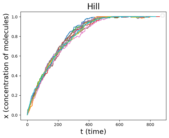
Figure 12: Stochastic Hill function, $N_{0}=2\Omega$, $k_{+}=k_{-}=\lambda_{-}=\lambda_{+}=1$, $\Omega=150$, $n=2$.

A similar derivation can be made for the case of a repressor, in this case, we would analyze a set of biochemical reactions similar to those we started in this section, and since the process is very similar (we omit the calculations) the Hill function would be obtained for a repressor and the same magnitude of the fluctuations although these would be given by

$$\eta(D)=\frac{1}{\Omega}\sqrt{{\sigma^{2}\left(\frac{s}{N_{0}}\right)}}=\frac{1}{\Omega}\sqrt{\frac{D(1-D)}{\Omega N_{0}^{d}K^{n}}}.$$ (49)

Because $H+D=1$, we can say that the fluctuations in $H$ and $D$ have the same magnitude.

We performed a simulation of the process from which we started using the Gillespie algorithm [11] (figure 12), where the initial condition of molecules $e$ is zero, which resembles the Hill function, although what really matters is the steady state.

Appendix B General Hill funtion

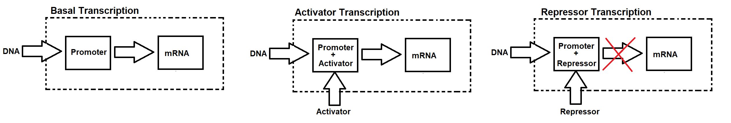
Figure 13: Genetic transcription.

In this appendix, we derive the Hill function exclusively when several proteins act as transcription factors. In figure 13 we can see that there are three ways in which mRA is synthesized: basal transcription is always present, whereas when transcription factors appear, transcription is faster (activator) or inhibits it (repressor). This model was inspired by [21]. For this, we assume that two types of proteins $P_{1}$ and $P_{2}$ act as transcription factors as activators and suppressors respectively, all the processes involved are given in the following biochemical reactions

1. Basal union: $G+P_{r}\stackbin[\lambda_{1}^{-}]{\lambda_{1}^{+}}{\rightleftarrows}GP_{r}$.

2. Activator transcription factor: $n_{1}P_{1}+P_{r}\stackbin[k_{1}^{-}]{k_{1}^{+}}{\rightleftarrows}P_{rp_{1}}$.

3. Suppressor transcription factor: $n_{2}P_{2}+P_{r}\stackbin[k_{2}^{-}]{k_{2}^{+}}{\rightleftarrows}P_{rp_{2}}$.

4. Binding with transcription factors: $G+P_{rp_{1}}\stackbin[\lambda_{2}^{-}]{\lambda_{2}^{+}}{\rightleftarrows}GP_{rp_{1}}$.

5. Basal mRNA synthesis: $GP_{r}\stackbin{\delta_{1}}{\rightarrow}R$.

6. mRNA synthesis with transcription factors: $GP_{rp_{1}}\stackbin{\delta_{2}}{\rightarrow}R$.

$G$ represents the gene, $P_{r}$ is the promoter, $R$ is the mAR, $GP_{r}$ is the gene binding to the promoter, $P_{rp_{1}}$ and $P_{rp_{2}}$ indicate when the transcription factor has joined the promoter. The first reaction at the top is a reversible process, indicating that the gene binds to the promoter regardless of the presence of transcription factors. The second reaction is also a reversible process, in which transcription factors bind to the promoter in such a way that they create a new molecule that accelerates mRNA synthesis. In the third reaction, a transcription factor creates a new molecule that cannot bind to a gene. In the fourth reaction, $G$ binds to the $P_{rp_{1}}$ molecule. The last two reactions indicate how mRNA is synthesized by a one-way process.

We used the law of mass action to build a set of differential equations that describe the concentrations of our system, where $g$ represents the gene concentration, $p_{r}$ is the promoter concentration, $r$ is the mAR concentration, $s_{1}$ is the concentration of $GP_{r}$, $s_{2}$ and $s_{3}$ at concentrations of $P_{rp_{1}}$ and $P_{rp_{2}}$ respectively, $s_{4}$ is the concentration of $GP_{rp_{1}}$. The differential equations we obtain are the following,

$$\frac{ds_{1}}{dt}= \lambda_{1}^{+}gp_{r}-\lambda_{1}^{-}s_{1}, \frac{ds_{2}}{dt}= k_{1}^{+}p_{1}^{n_{1}}p_{r}-k_{1}^{-}s_{2}-\lambda_{2}^{+}gs_{2}+\lambda_{1}^{-}s_{4},$$

$$\frac{ds_{3}}{dt}= k_{2}^{+}p_{2}^{n_{2}}p_{r}-k_{2}^{-}s_{3}, \frac{ds_{4}}{dt}= \lambda_{2}^{+}gs_{2}-\lambda_{1}^{-}s_{4},$$

$$\frac{dp_{r}}{dt}= -\lambda_{1}^{+}gp_{r}+\lambda_{1}^{-}-k_{1}^{+}p_{1}^{n_{1}}+k_{1}^{-}p_{r}-k_{2}^{+}p_{2}^{n_{2}}+k_{2}^{-}p_{r}, \frac{dr}{dt}= \delta_{1}s_{1}+\delta_{2}s_{4},$$ (50)

From these differential equations, we can see that we have a conserved quantity, and that the initial concentration of the promoters is constant, $p_{0}=p_{r}+s1+s2+s3+s4$. Of the reactions that we have, we consider that the first 4 are practically in equilibrium, so the first four differential equations are considered in equilibrium, from which we obtain the following conditions

$$s_{1}= \frac{\lambda_{1}^{+}}{\lambda_{1}^{-}}gp_{r}=\lambda_{1}gp_{r}, s_{2}= \frac{k_{1}^{+}}{k_{1}^{-}}p_{1}^{n_{1}}p_{r}=\frac{p_{1}^{n_{1}}}{K_{1}^{n_{1}}}p_{r},$$

$$s_{3}= \frac{k_{2}^{+}}{k_{2}^{-}}p_{2}^{n_{2}}p_{r}=\frac{p_{2}^{n_{2}}}{K_{2}^{n_{2}}}p_{r}, s_{4}= \frac{\lambda_{2}^{+}}{\lambda_{2}^{-}}gs_{2}=\lambda_{2}gs_{2}.$$ (51)

Our goal is to find a relationship that describes $s_{1}$ and $s_{4}$ in terms of transcription factors and basal synthesis since these are closely related to mRNA synthesis as can be seen in (50 ), then with the help of the above relations we can write the following

$$H_{1}= \frac{s_{1}}{p_{0}}=\frac{s_{1}}{p_{r}+s_{1}+s_{2}+s_{3}+s_{4}}, H_{2}=\frac{s_{4}}{p_{0}}=\frac{s_{4}}{p_{r}+s_{1}+s_{2}+s_{3}+s_{4}},$$ (52)

when evaluating the quantities obtained in (51) these relations we obtain

$$H_{1}= \frac{\lambda_{1}g}{1+\lambda_{1}g+\frac{p_{1}^{n_{1}}}{K_{1}^{n_{1}}}+\frac{p_{2}^{n_{2}}}{K_{2}^{n_{2}}}+\lambda_{2}g\frac{p_{1}^{n_{1}}}{K_{1}^{n_{1}}}}, H_{2}=\frac{\lambda_{2}g\frac{p_{1}^{n_{1}}}{K_{1}^{n_{1}}}}{1+\lambda_{1}g+\frac{p_{1}^{n_{1}}}{K_{1}^{n_{1}}}+\frac{p_{2}^{n_{2}}}{K_{2}^{n_{2}}}+\lambda_{2}g\frac{p_{1}^{n_{1}}}{K_{1}^{n_{1}}}}.$$ (53)

Remember that the synthesis of the mRNA is given by the term $\delta_{1}s_{1}+\delta_{2}s_{4}$, so now we will have

$$\delta_{1}s_{1}+\delta_{2}s_{4}=\delta_{1}p_{0}\frac{s_{1}}{p_{0}}+\delta_{2}p_{0}\frac{s_{4}}{p_{0}}=\delta_{1}p_{0}H_{1}+\delta_{2}p_{0}H_{2}=H,$$ (54)

where

$$H=\frac{\delta_{1}p_{0}\lambda_{1}g+\delta_{2}p_{0}\lambda_{2}g\frac{p_{1}^{n_{1}}}{K_{1}^{n_{1}}}}{1+\lambda_{1}g+\frac{p_{1}^{n_{1}}}{K_{1}^{n_{1}}}+\frac{p_{2}^{n_{2}}}{K_{2}^{n_{2}}}+\lambda_{2}g\frac{p_{1}^{n_{1}}}{K_{1}^{n_{1}}}}=\frac{\beta_{0}K_{0}+\beta_{11}\frac{p_{1}^{n_{1}}}{K_{1}^{n_{1}}}}{1+K_{0}+\beta_{21}\frac{p_{1}^{n_{1}}}{K_{1}^{n_{1}}}+\beta_{22}\frac{p_{2}^{n_{2}}}{K_{2}^{n_{2}}}},$$ (55)

($\beta_{0}=\delta_{1}p_{0}$, $K_{0}=\lambda_{1}g$, $\beta_{11}=\delta_{2}p_{0}\lambda_{2}g$, $\beta_{21}=(1+\lambda_{2}g)$, $\beta_{22}=1$). The function $H$ that we defined corresponds to the Hill function of our system, which indicates how the ARm is synthesized in terms of the transcription factors $P_{1}$ and $P_{2}$, in addition to a basal constant $K_{0}$. $\beta_{0}K_{0}$ denotes the basal synthesis rate. Now we can give a generalization of this expression, for this we suppose that we have a system with $m$ proteins that acts both as activators or suppressors, then our generalized Hill function ($H_{g}$) will be of the form

$$H_{g}=\frac{\beta_{0}K_{0}+\sum_{j}\beta_{1j}\left(\frac{p_{j}^{n_{j}}}{K_{j}^{n_{j}}}\right)^{q}}{1+K_{0}+\sum_{j}\beta_{2j}\frac{p_{j}^{n_{j}}}{K_{j}^{n_{j}}}},$$ (56)

we added $q$ to the numerator because if the protein acts as an activator, $q=1$, whereas if it acts as a suppressor, $q=0$. In this way, we have made a generalization of the Hill function, which will be very useful for analyzing any transcription-translation module in which many proteins participate. We can even introduce stochastic corrections to this Hill function, it will only be necessary to change to $p_{j}^{n_{j}}$ as follows

$$p_{j}^{n_{j}}\rightarrow p_{j}^{n_{j}}+\frac{1}{2}\sigma^{2}(p_{j},p_{j})n_{j}(n_{j}-1)p_{j}^{n_{j}-2},$$ (57)

This change is made according to the manner in which the Hill function with stochastic corrections is obtained.

Appendix C Hill function in a stochastic process

A methodology that explains how to properly introduce a Hill function in any stochastic biochemical reaction, such that the result can be generalized to other types of chemical reaction networks, is needed. To carry out the derivation, we rely on the ideas already presented up to this point and [7], where a separation is made between slow and fast variables. For our derivation, we first suppose that the probability distribution of our system is composed of the multiplication of a stationary part and a dynamic part, in such a way that we will have something of the following form

$$P(\mathbf{x},t)=P_{s}(x_{1},..,x_{s})P(x_{s+1},...,x_{l},t),$$ (58)

in [7] conditional probabilities are used, but because we directly consider that a part of the process is stationary, a separation between them can be made; in this case, we can assume that it is stationary because the concentrations of the variables associated with it tend to be very fast and asymptotically to the stationary value (the behavior of the Hill function). Under these considerations, the master equation of the system will be divided into a dynamic and stationary part that will be as follows

$$P_{s}(S_{1},..,S_{s})\frac{dP(S_{s+1},...,S_{j},t)}{dt}= \Omega\sum_{i}\left(t_{i}^{-}(S_{j}+\Gamma_{ji})P_{s}(S_{1}+\Gamma_{ii},..,S_{s}+\Gamma_{si})P(S_{s+1}+\Gamma_{s+1,i},...S_{j}+\Gamma_{j,i},t)\right.$$

$$-t_{i}^{+}(S_{j})P_{s}(S_{1},..,S_{s})P(S_{s+1},...,S_{j},t)$$

$$+t_{i}^{+}(S_{j}-\Gamma_{ji})P_{s}(S_{1}-\Gamma_{ii},..,S_{s}-\Gamma_{si})P(S_{s+1}-\Gamma_{s+1,i},...S_{j}$$

$$-\left.\Gamma_{j,i},t)-t_{i}^{-}(S_{j})P_{s}(S_{1},..,S_{s})P(S_{s+1},...,S_{j},t)\right),$$

$$P(S_{s+1},...,S_{j},t)\frac{dP_{s}(S_{1},..,S_{s})}{dt}= \Omega\sum_{i=rap}\left(t_{i}^{-}(S_{j}+\Gamma_{ji})P_{s}(S_{1}+\Gamma_{ii},..,S_{s}+\Gamma_{si})P(S_{s+1}+\Gamma_{s+1,i},...S_{j}+\Gamma_{j,i},t)\right.$$

$$-t_{i}^{+}(S_{j})P_{s}(S_{1},..,S_{s})P(S_{s+1},...,S_{j},t)$$

$$+t_{i}^{+}(S_{j}-\Gamma_{ji})P_{s}(S_{1}-\Gamma_{ii},..,S_{s}-\Gamma_{si})P(S_{s+1}-\Gamma_{s+1,i},...S_{j}$$

$$-\left.\Gamma_{j,i},t)-t_{i}^{-}(S_{j})P_{s}(S_{1},..,S_{s})P(S_{s+1},...,S_{j},t)\right)=0.$$ (59)

(Note that only fast reactions are considered in the second equation) Remember that the stationary part is the one associated with the Hill function, that is, this part is given by the following reaction

$$p+ne\stackbin[k_{-}]{k_{+}}{\rightleftarrows}pe_{n}.$$ (60)

These reactions are generally fast; therefore, the Hill function is determined if a deterministic analysis is performed. However, because we are using a stochastic approach, we would have to proceed in another way. Assuming that we are already in the stationary state, from these reactions and with the help of (59) we would obtain something similar to the following

$$k_{-}(s+1)P_{s}(e-n,p-1,s+1)-k_{+}p\frac{e!}{(e-n)!}\frac{1}{\Omega^{n}}P_{s}(e,p,s)+$$

$$k_{+}(p+1)\frac{(e+n)!}{e!}\frac{1}{\Omega^{n}}P_{s}(e+n,p+1,s-1)-k_{-}sP_{s}(e,p,s)=0.$$ (61)

($e$, $p$ and $s$ are the number of molecules $e$, $p$ and $pe_{n}$ respectively) Now, the question is what to do with this equation and how the Hill function would emerge, and there are two methods, as we will see below.

C.0.1 Exact Hill function

In this first derivation, from the equation (61) a stationary distribution is obtained, we use the method that we explained to obtain it,

$$P_{s}(e,p,s) =\left(\frac{1}{\Omega^{n}}\frac{k_{+}}{k_{-}}\braket{\frac{e!}{(e-n)!}}_{e}\right)^{s}\frac{N_{0}!}{s!(N_{0}-s)!}P_{s}(0).$$ (62)

Now we average the first equation of (59) with respect to this stationary distribution, we define the average with respect to the stationary part as $\braket{{t}^{\pm}}_{S}$ of this way our first equation becomes

$$\frac{dP(S_{s+1},...,S_{j},t)}{dt}=\Omega\sum_{i} \left(\braket{t_{i}^{-}(\mathbf{S}+\Gamma_{i})}_{s}P(S_{s+1}+\Gamma_{s+1,i},...S_{j}+\Gamma_{j,i},t)-\braket{t_{i}^{+}(\mathbf{S})}_{s}P(S_{s+1},...,S_{j},t)\right.$$

$$+\left.\braket{t_{i}^{+}(\mathbf{S}-\Gamma_{i})}_{s}P(S_{s+1}-\Gamma_{s+1,i},...S_{j}-\Gamma_{j,i},t)-\braket{t_{i}^{-}\mathbf{S}}_{s}P(S_{s+1},...,S_{j},t)\right),$$ (63)

This equation was used to model the dynamics of this type of system; only now are the reaction rates averaged with respect to the stationary part, for more details on the developments that can be reviewed [7]. Hill functions are expected to appear in the averages with respect to the stationary part, as observed in the case of Toggle Switch. However, because some averages would appear within this expression, it is not recommended to use Gillespie’s algorithm; however, we can still find the average of the concentrations and quantify the intrinsic fluctuations if the deterministic approach and dissipation fluctuation theorem are used.

C.0.2 Hill function variants

Assumptions
System Size	Distribution	Hill Function Type
X	X	Stochastic
X	✓	Semi-stochastic
✓	X	Semi-deterministic
✓	✓	Deterministic

Table 1: Assumptions table.

In the case in which we want to do Gillespie-type simulations, and also explain how the deterministic Hil function appears, we can derive another type of Hill functions, from (61) we find the following two relations

$$s+1= p\frac{1}{K^{n}}\frac{e!}{(e-n)!}\frac{1}{\Omega^{n}}\frac{P(e,p,s)}{P(e-n,p-1,s+1)}, s=(p+1)\frac{1}{K^{n}}\frac{(e+n)!}{e!}\frac{1}{\Omega^{n}}\frac{P(e+n,p+1,s-1)}{P(e,p,s)},$$ (64)

We define $\frac{k_{-}}{k_{-}}=K^{n}$. Several assumptions can be made to determine the Hill function, including the size of the system and/or shape of the distribution (these conditions were chosen to treat the previous equations as algebraic), as outlined in Table 1. In this table, we have four types of Hill functions; its type depends on the type of assumptions that are considered: in the case that we do not make any, we have a stochastic case; when considerations are made in the probability distribution, we have a semi-stochastic case, and so on. These names were chosen because of the degree of relevance of the components to each formalism. For example, in the stochastic case, one mainly considers the master equation, which is a differential equation of distributions.

Semi-deterministic case

First, we analyze the semi-deterministic case, assuming that the system is sufficiently large. The probability distribution can then be approximated as $\frac{P(e,p,s)}{P(e-n,p-1,s+1)}\approx 1$. We consider two cases because we have two expressions in (64) and $p+s=N_{0}$:

1. For this case, we use the first equation of (64), $s$ and $N_{0}$ are very large (because the system is large) so $s+1\approx s$ and also $\ frac{P(e,p,s)}{P(e-n,p-1,s+1)}\approx 1$, so we would have

   $$s=p\frac{1}{K^{n}}\frac{e!}{(e-n)!}\frac{1}{\Omega^{n}},$$ (65)

   substituting in the definition of the Hill function $H=\frac{s}{s+p}$ we obtain,

   $$H_{1}=\frac{e!}{\Omega^{n}K^{n}(e-n)!+e!}.$$ (66)

2. For this other case, we use the second equation of (64), $p$ and $N_{0}$ are very large (because the system is large) so $p+1\approx p$, said of otherwise $s$ has to be very small because we have the relation $N_{0}=s+p$, furthermore, we suppose $\frac{P(e+n,p+1,s-1)}{P(e,p,s)}\approx 1$, so we would have

   $$s=p\frac{1}{K^{n}}\frac{(e+n)!}{e!}\frac{1}{\Omega^{n}},$$ (67)

   Substituting in the definition of the Hill function we get,

   $$H_{2}=\frac{(e+n)!}{\Omega^{n}K^{n}e!+(e+n)!}.$$ (68)

In this way we have obtained our Hill function for two regions, so we can say that one is valid when $s$ is small and the other when it is large, so we define a Hill function for all possible values of $s$ as follows

$$H_{sd}=\frac{e!}{\Omega^{n}K^{n}(e-n)!+e!}+\left(\frac{(e+n)!}{\Omega^{n}K^{n}e!+(e+n)!}-\frac{e!}{\Omega^{n}K^{n}(e-n)!+e!}\right)\theta\left(\frac{1}{2}-\frac{s}{N_{0}}\right),$$ (69)

A Heavennside function was introduced to separate the two regions of the function, which relies on $H_{1}$ or $H_{2}$ depending on the value of $s$, thus covering all possible values of $s$. We obtained our semi-deterministic Hill function, which is semi-deterministic because the probability considerations are almost deterministic. Also, when $e$ and/or $\Omega$ get very large

$$H_{sd}\approx H_{d}=\frac{\frac{e^{n}}{\Omega^{n}}}{K^{n}+\frac{e^{n}}{\Omega^{n}}},$$ (70)

A Heavennside function was introduced to separate the two regions of the function, which relies on $H_{1}$ or $H_{2}$ depending on the value of $s$, thus covering all possible values of $s$. We obtained our semi-deterministic Hill function, which is semi-deterministic because the probability considerations are almost deterministic. In addition, when $e$ and/or $\Omega$ become very large.

Stochastic case

In the case that we want to use a stochastic Hill function, we can construct a completely stochastic one, for this we return to the relations found in (61) but without making any assumptions, we operate in a similar way to the case above, to cover the different values of $s$, we finally obtain our stochastic Hill function

$$H_{s} =\frac{e!}{\Omega^{n}K^{n}(e-n)!\frac{P(e-n,s+1)}{P(e,s)}+e!}$$

$$+\left(\frac{(e+n)!}{\Omega^{n}K^{n}e!\frac{P(e,s)}{P(e+n,s-1)}+(e+n)!}-\frac{e!}{\Omega^{n}K^{n}(e-n)!\frac{P(e-n,s+1)}{P(e,s)}+e!}\right)\theta\left(\frac{1}{2}-\frac{s}{N_{0}}\right).$$ (71)

This is the stochastic Hill function, which depends on the probability distribution of the system and, using this function as defined within the master equation, becomes more complex.

Semi-Stochastic case

Because it is more complicated to use the Hill function in a stochastic process, we approximated the probabilities. So we suppose the following

$$\frac{P(e+e_{1},s+s_{1})}{P(e,s)}\approx e^{-\left(\frac{e_{1}+s_{1}}{\Omega}\right)},$$ (72)

We used this approximation because when the system is large, the binomial distribution that appears in the steady state tends to be a Poisson distribution, and when $\Omega$ is sufficiently large, we find the deterministic assumption of cases a) and b). Substituting these relations in the previous equation we obtain our semi-stochastic Hill function, because we make a consideration on the distribution $P(e,s)$,

$$H_{ss} =\frac{e!}{e^{\left(\frac{n-1}{\Omega}\right)}\Omega^{n}K^{n}(e-n)!+e!}+\left(\frac{(e+n)!}{e^{\left(\frac{n-1}{\Omega}\right)}\Omega^{n}K^{n}e!+(e+n)!}-\frac{e!}{e^{\left(\frac{n-1}{\Omega}\right)}\Omega^{n}K^{n}(e-n)!+e!}\right)\theta\left(\frac{1}{2}-\frac{s}{N_{0}}\right).$$ (73)

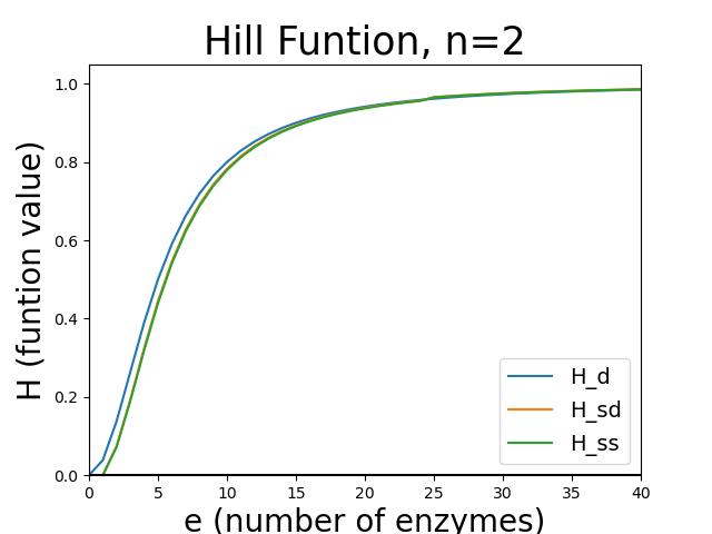
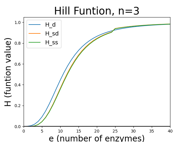
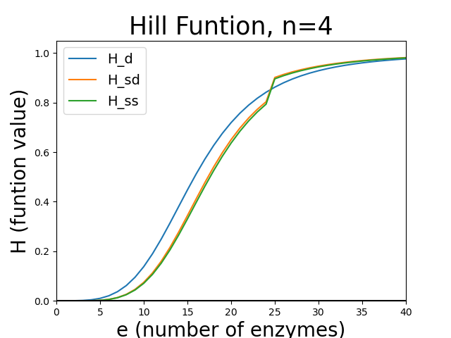
Figure 14: Hill functions. In this figure the deterministic $H_{d}$, semi-deterministic $H_{sd}$ and semi-stochastic Hill function $H_{ss}$ is plotted for different values of $n$, with $K=0.01$, $\Omega=50$.

We call this function the semi-stochastic Hill function because we made a consideration only on the probability distribution, this function coincides with the semi-deterministic when $n=1$ or when the value of $\Omega$ is very great,

$$\lim_{\Omega\to\infty}H_{ss}=\frac{\frac{e^{n}}{\Omega^{n}}}{K^{n}+\frac{e^{n}}{\Omega^{n}}}=H_{d},$$ (74)

Therefore, to perform simulations of a certain stochastic system and when the system size is small, we recommend using the semi-stochastic Hill function because it represents the system more faithfully. This function is considerably easier to use in stochastic simulations.

To observe the behavior of the Hill functions that we have calculated, $H_{d}$, $H_{sd}$ and $H_{ss}$, we made some graphs that can be seen in figure 14, in which we notice that when $n=1$ it is observed that the three functions are practically the same, and when the value of $e$ increases, the values of the three are almost identical, whereas at small values, there is a large difference, as shown in the figures. Another feature they share is that they all practically become step functions when $n$ is large. However, the location where the step varies, because factorials appear is semi-deterministic or semi-stochastic.

The considerations we have made for the appearance of Hill functions may not be completely fulfilled (even more so when the size of the system is small). Therefore, if one wants a process that is as realistic as possible, it is better to use the relations presented at the beginning of this subsection. However, other complications are possible if the constants are unknown in detail. Therefore, the best approach would be to use an exact derivation.

References

- [1]
- [2] Roces, M. E. Á. B., Martínez-García, J. C., Dávila-Velderrain, J., Domínguez-Hüttinger, E., & Martínez-Sánchez, M. E. (2018). Modeling Methods for Medical Systems Biology.
- [3] Alon, U. (2019). An introduction to systems biology: design principles of biological circuits. CRC press.
- [4] Walczak, A. M., Mugler, A., & Wiggins, C. H. (2012). Analytic methods for modeling stochastic regulatory networks. Computational Modeling of Signaling Networks, 273-322.k.
- [5] Paulsson, J. (2005). Models of stochastic gene expression. Physics of life reviews, 2(2), 157-175.
- [6] Thomas, P., Straube, A. V., & Grima, R. (2012). The slow-scale linear noise approximation: an accurate, reduced stochastic description of biochemical networks under timescale separation conditions. BMC systems biology, 6(1), 1-23.
- [7] Gómez-Uribe, C. A., Verghese, G. C., & Tzafriri, A. R. (2008). Enhanced identification and exploitation of time scales for model reduction in stochastic chemical kinetics. The Journal of chemical physics, 129(24), 244112.
- [8] Santillán, M. (2014). Chemical kinetics, stochastic processes, and irreversible thermodynamics (Vol. 2014). Heidelberg: Springer.
- [9] Gardiner, C.W., et al.: Handbook of Stochastic Methods vol. 3. Springer, Berlin; New York (2004)
- [10] Thomas, P., Matuschek, H., & Grima, R. (2013). How reliable is the linear noise approximation of gene regulatory networks?. BMC genomics, 14(4), 1-15.
- [11] Gillespie, D. T. (1976). A general method for numerically simulating the stochastic time evolution of coupled chemical reactions. Journal of computational physics, 22(4), 403-434.
- [12] Lecca, P. (2013). Stochastic chemical kinetics.
- [13] Anderson, D. F., Craciun, G., & Kurtz, T. G. (2010). Product-form stationary distributions for deficiency zero chemical reaction networks. Bulletin of mathematical biology, 72(8), 1947-1970.
- [14] GRIMA, Ramon. Linear-noise approximation and the chemical master equation agree up to second-order moments for a class of chemical systems. Physical Review E, 2015, vol. 92, no 4, p. 042124.
- [15] Gomez-Uribe, C. A., & Verghese, G. C. (2007). Mass fluctuation kinetics: Capturing stochastic effects in systems of chemical reactions through coupled mean-variance computations. The Journal of chemical physics, 126(2), 024109.
- [16] Scott, M. (2012). Applied stochastics Processes in science and engineering
- [17] Iglesias, P. A., & Ingalls, B. P. (Eds.). (2010). Control theory and systems biology. MIT press.
- [18] Elowitz, M., and Leibler, S. (2000). A synthetic oscillatory network of transcriptional regulators. Nature 403:335–338.
- [19] Loinger, A., & Biham, O. (2007). Stochastic simulations of the repressilator circuit. Physical Review E, 76(5), 051917.
- [20] Loinger, A., Lipshtat, A., Balaban, N. Q., & Biham, O. (2007). Stochastic simulations of genetic switch systems. Physical Review E, 75(2), 021904.
- [21] Del Vecchio, D., & Murray, R. M. (2014). Biomolecular feedback systems. In Biomolecular Feedback Systems. Princeton University Press.