[1]\fnmKeqin \surLiu \equalcontBoth authors contributed equally to this work.

\equalcont

Both authors contributed equally to this work.

1]\orgdivDepartment of Mathematics, \orgnameNanjing University, \orgaddress\cityNanjing, \postcode210093, \countryChina

PCL-Indexability and Whittle Index for Restless Bandits with General Observation Models

kqliu@nju.edu.cn    \fnmChengzhong \surZhang 171840780@smail.nju.edu.cn [
Abstract

In this paper, we consider a general observation model for restless multi-armed bandit problems. The operation of the player needs to be based on certain feedback mechanism that is error-prone due to resource constraints or environmental or intrinsic noises. By establishing a general probabilistic model for dynamics of feedback/observation, we formulate the problem as a restless bandit with a countable belief state space starting from an arbitrary initial belief (a priori information). We apply the achievable region method with partial conservation law (PCL) to the infinite-state problem and analyze its indexability and priority index (Whittle index). Finally, we propose an approximation process to transform the problem into which the AG algorithm of Niño-Mora and Bertsimas for finite-state problems can be applied to. Numerical experiments show that our algorithm has an excellent performance.

keywords:
restless bandit, POMDP, countable state space, partial conservation law, Whittle index

1 Introduction

The multi-armed bandit (MAB) problem is a classic reinforcement learning problem that involves a learner making choices among actions with uncertain/random rewards in order to maximize the expected return in long-term. The MAB problem is often associated with the important exploration-exploitation tradeoff and was initially proposed by  Robbins [29]. As a classic stochastic scheduling problem, the MAB problem has a wide range of practical applications, including clinical trials, communication transmission, recommendation systems, and financial investments [15, 3]. In the medical field, the MAB model is used to study clinical trials with different treatment effects [28], while in the financial field, the MAB model is used to design financial investment portfolios [17, 31]. In the field of stochastic scheduling, the MAB model is used to control the dynamic allocation of resources to different projects and provide corresponding decision-making strategies [9]. Therefore, finding efficient optimization algorithms for the MAB problem is of great practical significance.

In the classic MAB problem, the MAB system has a total of $N$ arms. After a player selected one of these arms and activated it, they will obtain a random reward related to the activated arm and its current state. In this process, all states are visible, and only the state of the arm being activated changes according to a Markov transition probability matrix. The goal of the MAB problem is to find a policy that maximizes the long-term cumulative reward. Gittins [15] demonstrated that the classic MAB problem can be solved optimally by an index policy, and the player only needs to activate the arm with the largest index at each moment. This index is also known as the Gittins index, and the proposed Gittins index greatly reduces the complexity of the algorithm for solving the optimal policy. After that, Whittle [35] extended the MAB problem to the restless MAB (RMAB) model, in which $K$ arms can be activated at each moment, and the arms at rest will also undergo state transitions over time. However, for the general RMAB problem, Papadimitriou and Tsitsiklis [27] showed that the computational complexity category of the optimal policy is PSPACE, which brings difficulties to the exploration of the problem. For this problem, Whittle [35] provides another way to assign state indexes by considering the Lagrangian dual function, which is called the Whittle index. The Whittle index policy, that is, activating the arm with the largest Whittle index at each time, has been proven to be the optimal policy of the RMAB under a relaxed constraint, which means that the player can choose to change the number of arms activated at each moment, but the number of arms activated at each moment is still $K$ on average/expectation. In addition, under certain conditions, the Whittle index policy has been proven to be asymptotically optimal by Weber and Weiss [34]. The establishment of Whittle index requires the so-called indexability, but not every RMAB problem is indexable. In fact, the establishment of indexability of most RMAB problems is not easy. For some special types of RMAB problems, indexability can be directly established, such as the dual-speed bandit problem and partially observable RMAB under perfect observation[16, 21]. Moreover, even if the problem is indexable, the calculation of the Whittle index and its optimality verification are also great challenges today. In the last 30 years, a large number of scholars have studied the RMAB problem and the Whittle index policy, established the indexability of some special categories of RMAB problems, and proved the optimality of the Whittle index in some cases [1]. The MAB problem and the RMAB problem are also described in detail in [14].

In practical applications, there exists a special class of RMAB problems, in which we cannot fully grasp the information of each arm at every moment, and can only observe the real state of the activated arm, while the state of the arm at rest is invisible. This type of RMAB belongs to partially observable MDP(POMDP) problems [33]. In situations where the actual state may be unknown, belief state becomes an alternative state metric. The belief state is a probability vector that an arm is currently in one of various possible states under the condition of all past information. It is a sufficient statistic for optimal decision-making [32]. For such partially observable RMAB problems, we hope to obtain Whittle index or its good approximation as a function of arm belief states. Liu and Zhao [21] established indexability and built a closed-form expression of Whittle indexes for the two-state scenario of this problem, and the Whittle index policy showed asymptotically optimal performance. Liu et al. [22] also proposed an error-prone observation model for this kind of problem, that is, the observer may have a certain probability to observe a false state. A classic application example of this type of problem is cognitive radio, whose spectrum access corresponds to the activation of the arm in the RMAB model. However, due to hardware constraints, the observation of spectrum access may be accompanied by errors [22, 36]. Liu [19] considered the perfect observation of such POMDP problems at any number of states, and gave a closed expression of the Whittle index under the concept of relaxed indexability. In these articles, the calculation of Whittle index is mainly using threshold policies and dynamic programming to analyze the value function. In this paper, we extend the above problems to the general imperfect observation model of partially observable RMABs for high-dimensional state spaces. We address this problem by defining an error matrix and a reward matrix to generalize it to the scenario of observations with arbitrary errors. However, generalization of errors will introduce nonlinear difficulties to the index calculation of the problem, which makes it not easy to directly use dynamic programming for key computations. Therefore, another approach was needed to address the problem.

In the field of stochastic optimization, an analysis method called "Achievable Region" emerged in the 1990s. Under the analysis framework of achievable regions, many stochastic optimization problems can be transformed into linear programming forms by defining performance measures for states under a given policy. At this point, the core of the problem is transformed into a mathematical representation of achievable regions. For the achievable region method, Coffman and Mitrani [7], Gelenbe and Mitrani [13], Federgruen and Groenevelt [10, 11] first considered the linear constraints between performance measures. They successfully characterized the polyhedral structure of the achievable region of the corresponding problem using the conservation law method and obtained a simple optimal policy structure. Bertsimas [4] summarized several types of random optimization problems, proposed constraints between performance measures for each type of problem, and characterized the corresponding achievable region. After that, Bertsimas and Niño-Mora [5] demonstrated that if performance measures in a stochastic and dynamic scheduling problem satisfy the so-called generalized conservation law (GCL), the achievable region of the problem is a polyhedron called extended polymatroid.They have also applied this method to several random scheduling problems, including modeling the classic MAB problem, and presented a low complexity adaptive greedy algorithm for calculating indexes. This algorithm was originally proposed by Tsoucas when solving the Klimov problem [18]. Niño-Mora has made outstanding contributions to the application of achievable regions and conservation law methods to RMAB problems. In 2001, Niño-Mora [23] relaxed the GCL restrictions, proposed the partial conservation law (PCL), and gave the PCL conditions satisfied by the RMAB problem, and similarly gave the calculation method of Whittle index. After that, Niño-Mora further expanded the method and presented a new AG algorithm. Under this algorithm, Niño-Mora [24] gave an economic explanation of the indexability of PCL, and interpreted the Whittle index as the optimal marginal cost rate. This way of modeling will bring great convenience to the research of the problem. More of his work is summarized in [26]. The application of the PCL framework to the RMAB problem is also heuristic. It provides sufficient conditions for establishing the indexability of the RMAB problem and an efficient Whittle index algorithm. This paper analyzes and discusses the belief state space in the case of imperfect observations, and gives the idea of the approximate state space. Although the number of states in the approximate state space may be very large, under the framework of PCL analysis, we can still obtain a simple algorithm for calculating the Whittle index. This algorithm solves the problem to which ordinary dynamic programming algorithms are difficult to apply. After obtaining the Whittle index algorithm, we compare the numerical simulation results of our Whittle index policy with the myopic policy, verifying the excellent performance of the Whittle index policy for the RMAB system under the condition that the PCL indexability is established.

Frostig and Weiss [12] in 2014 presented four different ways to prove the optimality of the Gittins index for the classic MAB problem, and generalized the GCL method to the countable state space, demonstrating that the Gittins index is still optimal for countable state spaces. In this paper, we will apply the PCL analysis framework to the RMAB problem with countable states, and use the weak duality theorem in infinite-dimensional linear programming [2]. We will discuss the optimality of the Whittle index for a specific problem by using similar arguments.

For the general partially and imperfectly observable RMAB problems, a relatively simple and effective optimization algorithm has not yet been proposed prior to this paper. Based on the theory of the Whittle index, we mathematically model the partially observable RMAB in the general context of imperfect observations, and present an effective algorithm for calculating the Whittle index under the framework of partial conservation laws. Numerical simulations have been conducted to verify the effectiveness of our algorithm and its superiority to the myopic policy.

2 Main Results

2.1 Model Formulation

In this section, we will formulate the RMAB problem as a POMDP problem under imperfect observations, that is, the entire bandit system is a partially observable Markov decision process. Assume the model has $N$ arms and the state space of the $i$th arm is $\mathcal{M}_{n}$. The whole state space is $\mathcal{M}=\bigcup_{n=1}^{N}\mathcal{M}_{n}$. At each moment, the actual state of each arm will undergo state transitions based on its own Markov probability transition matrix, and we will select $K$ arms to activate. For those activated arms, we can observe their states and obtain the reward they bring in specific states, but in this process, the observation is accompanied by errors, that is, we will observe states different from the actual states with certain probabilities. For those arms that are not activated, we can neither observe their states nor get reward from them, but their states still transit over time. Let $S_{n}(t),O_{n}(t)$ be the real and observed state of arm $n$ in slot $t$ and $A(t)$ the active set in slot $t$. First consider a single-arm process. Suppose the transition matrix, error matrix and reward matrix are $P=\{p_{ij}\}_{\mathcal{M}\times\mathcal{M}}$, $E=\{\varepsilon_{ij}\}_{\mathcal{M}\times\mathcal{M}}$ and $R=\{r_{ij}\}_{\mathcal{M}\times\mathcal{M}}$ respectively. For error matrix, $\varepsilon_{ij}$ represents the probability that the observed state is $j$ when the real state is $i$, that is, $\varepsilon_{ij}=P(O=j|S=i)$, while $r_{ij}$ represents the reward obtained when the real state is $i$ and the observed state is $j$. Denoted by $\Omega=\{(\omega_{1},\cdots,\omega_{M})|\sum_{i=1}^{M}\omega_{i}=1,\omega_{i}\geq 0,1\leq i\leq M\}$ the belief space, for each $\boldsymbol{\omega}(t)=(\omega_{1}(t),\cdots,\omega_{M}(t))\in\Omega$, $\omega_{i}(t)$ represents the conditional probability that the real state is $i$ in slot $t$. If the current belief state is $(\omega_{1},\cdots,\omega_{M})$, the current expected reward is $\sum_{i=1}^{M}\omega_{i}(\sum_{j=1}^{M}\varepsilon_{ij}r_{ij})$. Imperfect observation means that after activating an arm, we may not be able to observe the real state, but can only receive a feedback related to the real state and reward. Assume that there are $L$ feedback states in total, and denote them by $F=\{f_{1},\cdots,f_{L}\}(L\leq M^{2})$. Define $\rho_{ij}=P(F(t)=j|S(t)=i)$. By Bayes rule, we have

$$P(S(t+1)=j|F(t)=i)=\frac{P(S(t+1)=j,F(t)=i)}{P(F(t)=i)}=\frac{\sum_{k=1}^{M}p_{kj}\rho_{ki}\omega_{k}}{\sum_{k=1}^{M}\rho_{ki}\omega_{k}}.$$ (1)

Thus the rule of belief update is

$$\boldsymbol{\omega}(t+1)=\begin{cases}(\frac{\sum_{i=1}^{M}p_{i1}\rho_{ij}\omega_{i}}{\sum_{i=1}^{M}\rho_{ij}\omega_{i}},\cdots,\frac{\sum_{i=1}^{M}p_{iM}\rho_{ij}\omega_{i}}{\sum_{i=1}^{M}\rho_{ij}\omega_{i}}),&\text{if active and }F(t)=j\\ \boldsymbol{\omega}(t)P,&\text{if passive}\end{cases}.$$ (2)

For example, if we view observed states as the only feedback, the feedback space is $F=\{\{O=1\},\cdots,\{O=M\}\}$. Thus the update rule is exactly

$$\boldsymbol{\omega}(t+1)=\begin{cases}(\frac{\sum_{i=1}^{M}p_{i1}\varepsilon_{ij}\omega_{i}}{\sum_{i=1}^{M}\varepsilon_{ij}\omega_{i}},\cdots,\frac{\sum_{i=1}^{M}p_{iM}\varepsilon_{ij}\omega_{i}}{\sum_{i=1}^{M}\varepsilon_{ij}\omega_{i}}),&\text{if active and }O(t)=j\\ \boldsymbol{\omega}(t)P,&\text{if passive}\end{cases}.$$ (3)

Another way to get feedback is when we cannot observe any state after activating an arm, but can get a certain reward, which is the feedback determined by the arm real state. In the case of having the information of the reward matrix, we have

$\displaystyle\rho_{ij}=$ $\displaystyle P(R(t)=j|S(t)=i)$
$\displaystyle=$ $\displaystyle\frac{P(R(t)=j,S(t)=i)}{P(S(t)=i)}$
$\displaystyle=$ $\displaystyle\frac{\sum_{k=1}^{M}P(R(t)=j,O(t)=k,S(t)=i)}{\omega_{i}}$
$\displaystyle=$ $\displaystyle\frac{\sum_{k=1}^{M}P(R(t)=j|O(t)=k,S(t)=i)P(O(t)=k|S(t)=i)\omega_{i}}{\omega_{i}}$
$\displaystyle=$ $\displaystyle\sum_{k=1}^{M}\mathbbm{1}(r_{ik}=j)\varepsilon_{ik}$

or $\rho_{ir}=\sum_{j=1}^{M}\mathbbm{1}(r_{ij}=r)\varepsilon_{ij}$. Thus we have

$\displaystyle\sum_{i=1}^{M}p_{i1}\rho_{ir}\omega_{i}={}$ $\displaystyle\sum_{i=1}^{M}p_{i1}(\sum_{j=1}^{M}\mathbbm{1}(r_{ij}=r)\varepsilon_{ij}\omega_{i})$
$\displaystyle={}$ $\displaystyle\sum_{i=1}^{M}\sum_{j=1}^{M}\mathbbm{1}(r_{ij}=r)p_{i1}\varepsilon_{ij}\omega_{i}$
$\displaystyle={}$ $\displaystyle\sum_{r_{ij}=r}p_{i1}\varepsilon_{ij}\omega_{i}.$ (4)

Similarly,

$$\sum_{i=1}^{M}\rho_{ij}\omega_{i}=\sum_{r_{ij}=r}\varepsilon_{ij}\omega_{i}.$$ (5)

Combining (2.1) and (5), the belief state update rule is

$$\boldsymbol{\omega}(t+1)=\begin{cases}(\frac{\sum_{r_{ij}=r}p_{i1}\varepsilon_{ij}\omega_{i}}{\sum_{r_{ij}=r}\varepsilon_{ij}\omega_{i}},\cdots,\frac{\sum_{r_{ij}=r}p_{iM}\varepsilon_{ij}\omega_{i}}{\sum_{r_{ij}=r}\varepsilon_{ij}\omega_{i}}),&\text{if active and }R(t)=r\\ \boldsymbol{\omega}(t)P,&\text{if passive}\end{cases}.$$ (6)

A more practical situation is that we can jointly obtain information from the observed state and the obtained reward. In this case, we can similarly give the belief update rule:

$$\boldsymbol{\omega}(t+1)=\begin{cases}(\frac{\sum_{i=1}^{M}p_{i1}\varepsilon_{ij}\omega_{i}\mathbbm{1}(r=r_{ij})}{\sum_{i=1}^{M}\varepsilon_{ij}\omega_{i}\mathbbm{1}(r=r_{ij})},\cdots,\frac{\sum_{i=1}^{M}p_{iM}\varepsilon_{ij}\omega_{i}\mathbbm{1}(r=r_{ij})}{\sum_{i=1}^{M}\varepsilon_{ij}\omega_{i}\mathbbm{1}(r=r_{ij})}),&\text{if active and }O(t)=j,\\ &R(t)=r(\exists i~{}s.t.~{}r_{ij}=r)\\ \boldsymbol{\omega}(t)P,&\text{if passive}\end{cases}.$$ (7)

For the restless multi-armed bandit model, the goal is to find a policy $\pi$ which maps the belief states of all arms into an active set $A(t)$ in slot $t$ that maximize the long-term expected discounted reward. In other words, if we denote the reward obtained by the $n$-th arm in slot $t$ by $R_{n}(t)$, then our objective is

$\displaystyle\max_{\pi}\mathbb{E}_{\pi}$ $\displaystyle\left[\sum_{t=1}^{+\infty}\beta^{t-1}\sum_{n=1}^{N}R_{n}(t)\bigg{|}\boldsymbol{\omega}_{1}(1),\cdots,\boldsymbol{\omega}_{n}(1)\right],$ (8)
$\displaystyle s.t.~{}|A(t)|=K,t\geq 1,$ (9)

where $0\leq\beta<1$ is the discount factor and $\boldsymbol{\omega}_{n}(t)$ is the belief state of arm $n$ in slot $t$. In this problem, the diversity of states, choices, errors makes the problem highly complex. In similar RMAB problems, searching for an easily computable priority index policy is the mainstream. Its main idea is to assign an index to the current state of each arm, and then activate those arms with larger indexes. Our goal is to provide a computationally efficient index policy for this model. The next part of this article will follow this idea and provide corresponding priority index policy and a detailed algorithm.

2.2 Whittle Index

Whittle relaxed the constraint on the number of arms activated in each slot, requiring that the expected number of arms activated per slot on average (in the sense of discounted time) is $K$, i.e.

$$\mathbb{E}_{\pi}\left[\sum_{t=1}^{+\infty}\beta^{t-1}\sum_{n=1}^{N}\mathbbm{1}(n\in A(t))\bigg{|}\boldsymbol{\omega}(1)\right]=\frac{K}{1-\beta}$$ (10)

or

$$\mathbb{E}_{\pi}\left[\sum_{t=1}^{+\infty}\beta^{t-1}\sum_{n=1}^{N}\mathbbm{1}(n\notin A(t))\bigg{|}\boldsymbol{\omega}(1)\right]=\frac{N-K}{1-\beta}.$$ (11)

where $\boldsymbol{\omega}(t)=(\boldsymbol{\omega}_{1}(t),\cdots,\boldsymbol{\omega}_{N}(t))$. Thus the Lagrange optimization problem can be written as

$$\max_{\pi}\mathbb{E}_{\pi}\left[\sum_{t=1}^{+\infty}\beta^{t-1}\sum_{n=1}^{N}(\mathbbm{1}(n\in A(t))R_{n}(t)+\lambda\mathbbm{1}(n\notin A(t)))\bigg{|}\boldsymbol{\omega}(1)\right].$$ (12)

The above problem can be decomposed into $N$ independent subproblems, that is, for any $1\leq n\leq N$,

$$\max_{\pi}\mathbb{E}_{\pi}\left[\sum_{t=1}^{+\infty}\beta^{t-1}(\mathbbm{1}(n\in A(t))R_{n}(t)+\lambda\mathbbm{1}(n\notin A(t)))\bigg{|}\boldsymbol{\omega}_{n}(1)\right].$$ (13)

The explanation of the optimization problem above is that for each arm, when it is passive, it will receive a subsidy $\lambda$. Since the problems above are independent, we just need to consider the single arm case. For notation simplicity, we drop the arm index from now on. In general, for a given arm, the optimal policy for the relaxed optimization problem divides the state space into two subset: active set $\mathcal{A}(\lambda)$ and passive set $\mathcal{P}(\lambda)$. Specifically, $\mathcal{P}(\lambda)$ contains all states in which the optimal choice is passive when the subsidy is $\lambda$. In particular, for a certain state $i$, if both active and passive action are optimal decisions, we also include state $i$ in $\mathcal{P}(\lambda)$, and $\mathcal{A}(\lambda)$ is the complement set of $\mathcal{P}(\lambda)$ in the whole state space. Under the concept of the passive set, the Whittle indexability can be stated as follows:

Definition 1 (Whittle Indexability).

An arm is indexable if the passive set $\mathcal{P}(\lambda)$ increases from $\emptyset$ to the whole state space as the subsidy $\lambda$ increases from $-\infty$ to $+\infty$. The RMAB problem is indexable if every decoupled problem is Whittle indexable.

Indexability states that, once a bandit is rested with subsidy $\lambda$, it will also be rested with $\lambda^{\prime}$ which is larger than $\lambda$. If the problem satisfies indexability, the Whittle index can be further defined:

Definition 2 (Whittle Index).

If an arm is indexable, the Whittle index $W(s)$ of the state $s$ is the infimum subsidy $\lambda$ that keeps state $s$ in the passive set $\mathcal{P}(\lambda)$. That is,

$$W(s)=\inf\{\lambda:s\in\mathcal{P}(\lambda)\}.$$

In other words, $W(s)$ is the infimum subsidy that makes it equivalent to make active or passive at state $s$. In addition, under the subsidy $W(s)$, both active and passive action are optimal for state $s$.

Under the definition of indexability and Whittle index, the Whittle index policy refers to assigning the Whittle index to the current state of each arm at each moment, and activating the $K$ arms of the largest indices. In fact, for the classic MAB problem, the Whittle index policy reduces to the Gittins index policy exactly.

2.3 Approximate State Space

Different from the perfect observation case, the update of the belief state is nonlinear in the imperfect observation case. This will make it difficult for us to use value functions and dynamic programming methods to analyze the problem. Given an initial belief state, it appears that the size of the belief state space will grow exponentially over time as all possible scenarios are continuously traversed and updated. Fortunately, however, a large number of numerical experiments have shown that in the sense of Euclidean norm approximation, the state space exhibits convergence after a sufficiently long iterative calculation. This will be discussed later. Note that the initial belief state is $\boldsymbol{\omega}$, $\{\mathcal{B}_{l}\}_{0\leq l\leq L}$is a list of operators defined by feedback states and state update rules, that is, when $1\leq l\leq L$, $\mathcal{B}_{l}\boldsymbol{\omega}$ is the update state caused by the $l$-th feedback state under active action, and $\mathcal{B}_{0}$ is the state update operator under passive action. In this paper, $\mathcal{B}_{0}\boldsymbol{\omega}=\boldsymbol{\omega}P$. To give the concept of approximate state space, we recursively define the $T$-step state space as follows:

Definition 3 (T-step state space).

Define

$$\Omega(T|\boldsymbol{\omega})=\begin{cases}\{\mathcal{B}_{l_{1}}\cdots\mathcal{B}_{l_{T}}\boldsymbol{\omega}:0\leq l_{1},\cdots,l_{T}\leq L\}\cup\Omega(T-1|\boldsymbol{\omega})&,T\geq 2\\ \{\mathcal{B}_{l}\boldsymbol{\omega}:0\leq l\leq L\}\cup\{\boldsymbol{\omega}\}&,T=1\end{cases}.$$

We call $\Omega(T|\boldsymbol{\omega})$ the $T$-step state space under the initial belief state $\boldsymbol{\omega}$.

Under the concept of the $T$-step state space, $\Omega(+\infty|\boldsymbol{\omega_{0}})$ is the belief space obtained by traversing all possible state update rules starting from the initial state $\boldsymbol{\omega_{0}}$. By the definition of the $T$-step state space, $\Omega(+\infty|\boldsymbol{\omega_{0}})$ is countable, and we can denote it by $\Omega(\boldsymbol{\omega_{0}})$. In the countable belief state space under consideration, we can treat the belief state as the actual state during the decision-making process, and perform a detailed analysis of the belief state in the POMDP framework. In this case, we must consider the probability transitions between belief states. Under policy $\pi$, let $p_{ij}(\pi)=P(\boldsymbol{\omega}(t+1)=\boldsymbol{\omega_{j}}|\boldsymbol{\omega}(t)=\boldsymbol{\omega_{i}})$ be the conditional probability of transition from state $\boldsymbol{\omega_{i}}$ to $\boldsymbol{\omega_{j}}$. Furthermore, due to the different actions of activation and passivity affecting state updates, decomposition of $p_{ij}(\pi)$ can be carried out. If $a(t)$ is an indicator of whether the arm is activated in slot $t$, that is, $a(t)=1$ when the active action is taken, otherwise $a(t)=0$, then we can define the transition probability of the belief state under different actions:

$\displaystyle p_{ij}^{0}(\pi)=P(\boldsymbol{\omega}(t+1)=\boldsymbol{\omega}_{j}|\boldsymbol{\omega}(t)=\boldsymbol{\omega}_{i},a(t)=0),$ (14)
$\displaystyle p_{ij}^{1}(\pi)=P(\boldsymbol{\omega}(t+1)=\boldsymbol{\omega}_{j}|\boldsymbol{\omega}(t)=\boldsymbol{\omega}_{i},a(t)=1).$ (15)

By (14)-(15) and Bayes rule, we have

$\displaystyle p_{ij}(\pi)$ $\displaystyle=P(\boldsymbol{\omega}(t+1)=\boldsymbol{\omega}_{j}|\boldsymbol{\omega}(t)=\boldsymbol{\omega}_{i})$ (16)
$\displaystyle=\frac{P(\boldsymbol{\omega}(t+1)=\boldsymbol{\omega}_{j},\boldsymbol{\omega}(t)=\boldsymbol{\omega}_{i})}{P(\boldsymbol{\omega}(t)=\boldsymbol{\omega}_{i})}$
$\displaystyle=\frac{\sum\limits_{a=0}^{1}P(\boldsymbol{\omega}(t+1)=\boldsymbol{\omega}_{j},\boldsymbol{\omega}(t)=\boldsymbol{\omega}_{i},a(t)=a)}{P(\boldsymbol{\omega}(t)=\boldsymbol{\omega}_{i})}$
$\displaystyle=\frac{\sum\limits_{a=0}^{1}P(\boldsymbol{\omega}(t)=\boldsymbol{\omega}_{i},a(t)=a)p_{ij}^{a}(\pi)}{P(\boldsymbol{\omega}(t)=\boldsymbol{\omega}_{i})}$
$\displaystyle=\sum\limits_{a=0}^{1}P(a(t)=a|\boldsymbol{\omega}(t)=\boldsymbol{\omega}_{i})p_{ij}^{a}(\pi).$

The elements in the probability transition matrix under passive action and active actions have the following more specific expressions:

$$p_{ij}^{0}=\begin{cases}1,&\text{if $\boldsymbol{\omega}_{j}=\boldsymbol{\omega}_{i}P$}\\ 0,&\text{otherwise}\end{cases}$$ (17)

and

$\displaystyle p_{ij}^{1}$ $\displaystyle=P(\boldsymbol{\omega}(t+1)=\boldsymbol{\omega}_{j}|\text{active and }\boldsymbol{\omega}(t)=\boldsymbol{\omega}_{i})$ (18)
$\displaystyle=\sum\limits_{\{l:\mathcal{B}_{l}\boldsymbol{\omega}_{i}=\boldsymbol{\omega}_{j},1\leq l\leq L\}}P(F(t)=l|\text{active and }\boldsymbol{\omega}(t)=\boldsymbol{\omega}_{i}).$

In the following sections, these two probability transition matrices will play an important role in the calculation of Whittle indices.

2.4 Two-Arm Problem and Achievable Region

With the rapid development of the field of stochastic optimization problems, quite a few effective methods have been found, and achievable region with conservation law methods is a great example. In articles such as [5, 23], Bertsimas and Niño-Mora et al. adopted the analytical framework of generalized conservation laws and partial conservation laws for the classical MAB and RMAB problems, respectively, and provided efficient index algorithms for the corresponding problems. This section will mainly apply the PCL framework adopted by Niño-Mora when analyzing the RMAB problem, and provide an appropriate model for our problem. Consider the single-arm process with $M$ states discussed in the previous section. For an initial belief state $\boldsymbol{\omega_{0}}$, let $\Omega(\boldsymbol{\omega_{0}})$ be the countable belief state space generated by iteratively updating $\boldsymbol{\omega_{0}}$ through state transitions. During the process of making the arm active or passive, since all belief states fall within $\Omega(\boldsymbol{\omega_{0}})$, the entire time period can be completely partitioned by the time intervals in which each state is located. In this scenario, define the performance indicator variables for each belief state as follows:

$$I_{\boldsymbol{\omega}}^{1}(t)=\begin{cases}1,&\text{if the arm is active in slot $t$ and its belief state is $\boldsymbol{\omega}$}\\ 0,&\text{otherwise}\end{cases}$$

and

$$I_{\boldsymbol{\omega}}^{0}(t)=\begin{cases}1,&\text{if the arm is passive in slot $t$ and its belief state is $\boldsymbol{\omega}$}\\ 0,&\text{otherwise}\end{cases}.$$

Furthermore, define the performance measures of belief state $\boldsymbol{\omega}$ as follows:

$$x_{\omega}^{a}(\pi)=\mathbb{E}_{\pi}\left[\sum_{t=0}^{+\infty}\beta^{t}I_{\boldsymbol{\omega}}^{a}(t)\right],\quad a=0,1$$ (19)
$$x_{\omega}^{a}(\pi,\boldsymbol{\omega}_{i})=\mathbb{E}_{\pi}\left[\sum_{t=0}^{+\infty}\beta^{t}I_{\boldsymbol{\omega}}^{a}(t)\bigg{|}\boldsymbol{\omega}(0)=\boldsymbol{\omega}_{i}\right],\quad a=0,1$$ (20)

where $\boldsymbol{\omega}(t)$ is the belief state of the arm in slot $t$. In Whittle’s relaxation, the Lagrangian multiplier $\lambda$ can be regarded as a subsidy when the arm is made passive. Thus the optimization objective of the partially observable RMAB problem with subsidy can be written as:

$\displaystyle\max_{\pi}$ $\displaystyle\sum\limits_{\boldsymbol{\omega}\in\Omega(\boldsymbol{\omega_{0}})}R_{\boldsymbol{\omega}}x_{\boldsymbol{\omega}}^{1}+\lambda\sum\limits_{\boldsymbol{\omega}\in\Omega(\boldsymbol{\omega_{0}})}x_{\boldsymbol{\omega}}^{0}$ (21)
subject to $\displaystyle x_{\boldsymbol{\omega}_{i}}^{1}+x_{\boldsymbol{\omega_{i}}}^{0}=e_{\boldsymbol{\omega}_{i}}+\sum\limits_{\boldsymbol{\omega_{j}}\in\Omega(\boldsymbol{\omega_{0}})}p_{ji}^{1}x_{\boldsymbol{\omega}_{i}}^{1}+\sum\limits_{\boldsymbol{\omega_{j}}\in\Omega(\boldsymbol{\omega_{0}})}p_{ji}^{0}x_{\boldsymbol{\omega}_{i}}^{0},\quad\forall\boldsymbol{\omega_{i}}\in\Omega(\boldsymbol{\omega_{0}})$
$\displaystyle x_{\boldsymbol{\omega}_{i}}^{1},x_{\boldsymbol{\omega}_{i}}^{0}\geq 0,\quad\forall\boldsymbol{\omega_{i}}\in\Omega(\boldsymbol{\omega_{0}})$

where $R_{\boldsymbol{\omega}}=\sum\limits_{i=1}^{M}\omega_{i}R_{i},\boldsymbol{\omega}=(\omega_{1},\cdots,\omega_{M})$, $p_{ij}^{a}$ are given by (17)-(18), $e_{\boldsymbol{\omega}_{i}}$ is the indicator whether the initial belief state is $\boldsymbol{\omega}_{i}$. Obviously, $R_{\boldsymbol{\omega}}$ is bounded above and we can assume $|R_{\boldsymbol{\omega}}|\leq C,\forall\boldsymbol{\omega}\in\Omega(\boldsymbol{\omega_{0}})$. For the equality constraints of this programming problem, it can be understood that the left side of the equation is a performance measure for state $\boldsymbol{\omega}_{i}$, while the right side of the equation is another way to evaluate the performance measure. That is, each occurrence of state $\boldsymbol{\omega}_{i}$ in the system is transitioned by a certain state $\boldsymbol{\omega}_{j}$. Therefore, the performance measure for state $\boldsymbol{\omega}_{i}$ can be represented by a combination of performance measures of other states. This model with subsidy can be explained more intuitively through a two-arm system. In the two-arm system, the first arm is the original arm, and its parameters are given in the above modeling, while the second arm has only one state 0. We refer to the first arm as the original arm and the second arm as the auxiliary arm. In every slot we choose one of the arms to activate. When the auxiliary arm is activated, we can get a fixed reward $\lambda$. In this way, the problem with subsidy can be seen as follows: activate an arm in the system in each slot, if the active arm is the auxiliary arm, the corresponding original arm is in the passive state and the subsidy $\lambda$ is obtained. Under such modeling, our goal is to find a policy to maximize the long-term expected discounted reward of the two-arm system under this policy. The objective function can also be written as

$$\max\limits_{\pi}\sum\limits_{\boldsymbol{\omega}\in\Omega(\boldsymbol{\omega_{0}})}R_{\boldsymbol{\omega}}x_{\boldsymbol{\omega}}^{1}(\pi)+\lambda x_{0}^{1}(\pi),$$

where $x_{0}^{1}(\pi)$ is the performance measure of state 0 being activated under policy $\pi$. Let $X$ be the set of all elements $(x_{0}^{1}(\pi),x_{\boldsymbol{\omega}}^{1}(\pi))_{\boldsymbol{\omega}\in\Omega(\boldsymbol{\omega_{0}})}$ as $\pi$ traverses the admissible policy set $\Pi$. We call $X$ the achievable region. Under this definition, the optimization objective function can be written as follows:

$$\quad\max_{(x_{0}^{1},x_{\boldsymbol{\omega}}^{1})\in X}\sum\limits_{\boldsymbol{\omega}\in\Omega(\boldsymbol{\omega_{0}})}R_{\boldsymbol{\omega}}x_{\boldsymbol{\omega}}^{1}+\lambda x_{0}^{1}.$$ (OPT)

The core of solving this optimization problem is to mathematically characterize the achievable region $X$. The so-called conservation law refers to the fact that for any $(x_{0}^{1},x_{\boldsymbol{\omega}}^{1})\in X$, these components may satisfy certain equality or inequality constraints. For the above model, a trivial equality constraint is $x_{0}^{1}+\sum\limits_{\boldsymbol{\omega}\in\Omega(\boldsymbol{\omega_{0}})}x_{\boldsymbol{\omega}}^{1}=\frac{1}{1-\beta}$. This is because the RMAB system has exactly one state in the active phase at each moment. In the following sections, we will further explore the connections between the performance measure of the two-arm system with countable states under the concept of achievable region.

2.5 Partial Conservation Law

In this section, we will explore the relationship between performance measures for each state in the two-arm system. To measure the performance of the original arm of the two-arm system under policy $\pi$, we define the following variables:

$\displaystyle T_{\boldsymbol{\omega}_{i}}^{\pi}$ $\displaystyle=\mathbb{E}_{\pi}\left[\sum\limits_{t=0}^{+\infty}\beta^{t}\mathbbm{1}(a(t)=1)\bigg{|}\boldsymbol{\omega}(0)=\boldsymbol{\omega}_{i}\right],\quad\boldsymbol{\omega_{i}}\in\Omega(\boldsymbol{\omega_{0}}),$ (22)
$\displaystyle R_{\boldsymbol{\omega}_{i}}^{\pi}$ $\displaystyle=\mathbb{E}_{\pi}\left[\sum\limits_{t=0}^{+\infty}\beta^{t}R_{\boldsymbol{\omega}(t)}\mathbbm{1}(a(t)=1)\bigg{|}\boldsymbol{\omega}(0)=\boldsymbol{\omega}_{i}\right],\quad\boldsymbol{\omega_{i}}\in\Omega(\boldsymbol{\omega_{0}}).$ (23)

$T_{\boldsymbol{\omega}_{i}}^{\pi}$ describes the total expected discounted time for the original arm to be activated in the two-arm system under policy $\pi$. Here we require that the policy $\pi$ only depends on the original arm. Similarly, $R_{\boldsymbol{\omega}_{i}}^{\Omega}$ represents the expected discounted total reward obtained by the two-arm system from the original arm under policy $\pi$. Therefore, $T_{\boldsymbol{\omega}_{i}}^{\pi}$ and $R_{\boldsymbol{\omega}_{i}}^{\pi}$ also have the following expressions:

$\displaystyle T_{\boldsymbol{\omega}_{i}}^{\pi}$ $\displaystyle=\sum\limits_{\boldsymbol{\omega}\in\Omega(\boldsymbol{\omega}_{0})}x_{\boldsymbol{\omega}}^{1}(\pi,\boldsymbol{\omega}_{i}),$ (24)
$\displaystyle R_{\boldsymbol{\omega}_{i}}^{\pi}$ $\displaystyle=\sum\limits_{\boldsymbol{\omega}\in\Omega(\boldsymbol{\omega}_{0})}R_{\boldsymbol{\omega}}x_{\boldsymbol{\omega}}^{1}(\pi,\boldsymbol{\omega}_{i}).$ (25)

Intuitively, if the problem is Whittle indexable, then the optimal policy must be to take active action for a subset of belief states in $\Omega(\boldsymbol{\omega_{0}})$ and to take passive action for the remaining belief states. For any $\Omega\subset\Omega(\boldsymbol{\omega_{0}})$, we call $\pi_{\Omega}$ an $\Omega$-priority policy, if the original arm takes active action when its current belief state falls into $\Omega$ and takes passive action when the state falls into $\Omega^{c}$. For $\Omega$-priority policy, we have

$\displaystyle T_{\boldsymbol{\omega}_{i}}^{\Omega}$ $\displaystyle=\mathbb{E}_{\pi_{\Omega}}\left[\sum\limits_{t=0}^{+\infty}\beta^{t}\mathbbm{1}(\boldsymbol{\omega}(t)\in\Omega)\bigg{|}\boldsymbol{\omega}(0)=\boldsymbol{\omega}_{i}\right],\quad\boldsymbol{\omega_{i}}\in\Omega(\boldsymbol{\omega_{0}}),$ (26)
$\displaystyle R_{\boldsymbol{\omega}_{i}}^{\Omega}$ $\displaystyle=\mathbb{E}_{\pi_{\Omega}}\left[\sum\limits_{t=0}^{+\infty}\beta^{t}R_{\boldsymbol{\omega}(t)}\mathbbm{1}(\boldsymbol{\omega}(t)\in\Omega)\bigg{|}\boldsymbol{\omega}(0)=\boldsymbol{\omega}_{i}\right],\quad\boldsymbol{\omega_{i}}\in\Omega(\boldsymbol{\omega_{0}}).$ (27)

From the above definition, we can easily give the following dynamic programming equations for these two variables:

$$T_{\boldsymbol{\omega}_{i}}^{\Omega}=\begin{cases}1+\beta\sum\limits_{\boldsymbol{\omega_{j}}\in\Omega(\boldsymbol{\omega_{0}})}p_{ij}^{1}T_{\boldsymbol{\omega}_{i}}^{\Omega},&\boldsymbol{\omega}_{i}\in\Omega\\ \beta\sum\limits_{\boldsymbol{\omega_{j}}\in\Omega(\boldsymbol{\omega_{0}})}p_{ij}^{0}T_{\boldsymbol{\omega}_{i}}^{\Omega}&\boldsymbol{\omega}_{i}\notin\Omega\end{cases}$$ (28)

and

$$R_{\boldsymbol{\omega}_{i}}^{\Omega}=\begin{cases}R_{\boldsymbol{\omega}_{i}}+\beta\sum\limits_{\boldsymbol{\omega_{j}}\in\Omega(\boldsymbol{\omega_{0}})}p_{ij}^{1}R_{\boldsymbol{\omega}_{i}}^{\Omega},&\boldsymbol{\omega}_{i}\in\Omega\\ \beta\sum\limits_{\boldsymbol{\omega_{j}}\in\Omega(\boldsymbol{\omega_{0}})}p_{ij}^{0}R_{\boldsymbol{\omega}_{i}}^{\Omega}&\boldsymbol{\omega}_{i}\notin\Omega\end{cases}.$$ (29)

If $\Omega(\boldsymbol{\omega_{0}})$ is a finite state space, we can directly solve for $T_{\boldsymbol{\omega_{i}}}$ and $R_{\boldsymbol{\omega_{i}}}$ from the two equation systems above. Specifically, if the auxiliary arm in the two-arm system is considered for illustration, then the arm has only one state 0 with $R_{0}=\lambda,p_{00}^{1}=p_{00}^{0}=1$. In this case, we have $T_{0}^{\{0\}}=\frac{1}{1-\beta}$ and $R_{0}^{\{0\}}=\frac{\lambda}{1-\beta}$. However, this poses difficulties for countable state spaces. To further investigate the properties of these variables, we define $V_{\boldsymbol{\omega_{i}}}^{\pi}$ as the expected discounted total reward obtained by the two-arm system starting from state $\boldsymbol{\omega_{i}}$ under policy $\pi$. There is a direct relation between these variables:

$$V_{\boldsymbol{\omega_{i}}}^{\pi}=R_{\boldsymbol{\omega_{i}}}^{\pi}+\lambda\left(\frac{1}{1-\beta}-T_{\boldsymbol{\omega_{i}}}^{\pi}\right).$$ (30)

Further, let $V_{\boldsymbol{\omega_{i}},0}^{\pi}$ and $V_{\boldsymbol{\omega_{i}},1}^{\pi}$ be the expected discounted total rewards of the two-arm system with the initial state $\boldsymbol{\omega_{i}}$ when taking the actions of being passive and active, respectively, then

$\displaystyle V_{\boldsymbol{\omega_{i}},0}^{\pi}=\lambda+\beta\sum\limits_{\boldsymbol{\omega_{j}}\in\Omega(\boldsymbol{\omega_{0}})}p_{ij}^{0}V_{\boldsymbol{\omega_{j}}}^{\pi},$ (31)
$\displaystyle V_{\boldsymbol{\omega_{i}},1}^{\pi}=R_{\boldsymbol{\omega_{i}}}+\beta\sum\limits_{\boldsymbol{\omega_{j}}\in\Omega(\boldsymbol{\omega_{0}})}p_{ij}^{1}V_{\boldsymbol{\omega_{j}}}^{\pi}.$ (32)

If, under the policy $\pi$, the expected discounted total reward obtained by active and passive actions are the same for the initial states $\boldsymbol{\omega_{i}}$, i.e., $V_{\boldsymbol{\omega_{i},0}}^{\pi}=V_{\boldsymbol{\omega_{i},1}}^{\pi}$, then we can simply calculate and obtain:

$$\lambda=\frac{R_{\boldsymbol{\omega_{i}}}+\beta\sum\limits_{\boldsymbol{\omega_{j}}\in\Omega(\boldsymbol{\omega_{0}})}(p_{ij}^{1}-p_{ij}^{0})R_{\boldsymbol{\omega_{j}}}^{\pi}}{1+\beta\sum\limits_{\boldsymbol{\omega_{j}}\in\Omega(\boldsymbol{\omega_{0}})}(p_{ij}^{1}-p_{ij}^{0})T_{\boldsymbol{\omega_{j}}}^{\pi}}.$$ (33)

The computation result of $\lambda$ gives us an intuitive construction form similar to the Whittle index. Further define:

$\displaystyle A_{\boldsymbol{\omega}_{i}}^{\Omega}$ $\displaystyle=1+\beta\sum\limits_{\boldsymbol{\omega_{j}}\in\Omega(\boldsymbol{\omega_{0}})}(p_{ij}^{1}-p_{ij}^{0})T_{\boldsymbol{\omega}_{j}}^{\Omega^{c}},$ (34)
$\displaystyle W_{\boldsymbol{\omega}_{i}}^{\Omega}$ $\displaystyle=R_{\boldsymbol{\omega}_{i}}+\beta\sum\limits_{\boldsymbol{\omega_{j}}\in\Omega(\boldsymbol{\omega_{0}})}(p_{ij}^{1}-p_{ij}^{0})R_{\boldsymbol{\omega}_{j}}^{\Omega^{c}}.$ (35)

Since $T_{\boldsymbol{\omega_{j}}}^{\Omega^{c}}$ and $R_{\boldsymbol{\omega_{j}}}^{\Omega^{c}}$ are bounded above, thus $A_{\boldsymbol{\omega_{i}}}$ and $W_{\boldsymbol{\omega_{i}}}$ are meaningful. For the auxiliary arm, we have $A_{0}^{\{0\}}=1$ and $W_{0}^{\{0\}}=\lambda$. Generally, we can extend these variables to the multi-arm case. Now assume there are two arms and their state spaces are $\Omega(\boldsymbol{\omega})$ and $\Omega^{\prime}(\boldsymbol{\omega}^{\prime})$ with $\Omega(\boldsymbol{\omega})\cap\Omega^{\prime}(\boldsymbol{\omega}^{\prime})=\emptyset$. Then for $\Omega\subset\Omega(\boldsymbol{\omega})$, $\Omega^{\prime}\subset\Omega^{\prime}(\boldsymbol{\omega}^{\prime})$ and $\boldsymbol{\omega_{i}}\in\Omega(\boldsymbol{\omega})$, we define $T_{\boldsymbol{\omega_{i}}}^{\Omega\cup\Omega^{\prime}}=T_{\boldsymbol{\omega_{i}}}^{\Omega},R_{\boldsymbol{\omega_{i}}}^{\Omega\cup\Omega^{\prime}}=R_{\boldsymbol{\omega_{i}}}^{\Omega},A_{\boldsymbol{\omega_{i}}}^{\Omega\cup\Omega^{\prime}}=A_{\boldsymbol{\omega_{i}}}^{\Omega}$ and $W_{\boldsymbol{\omega_{i}}}^{\Omega\cup\Omega^{\prime}}=W_{\boldsymbol{\omega_{i}}}^{\Omega}$. Niño-Mora originally provided the relationship between the variables $T_{\boldsymbol{\omega_{i}}}^{\Omega}$, $R_{\boldsymbol{\omega_{i}}}^{\Omega}$, $A_{\boldsymbol{\omega_{i}}}^{\Omega}$ and $W_{\boldsymbol{\omega_{i}}}^{\Omega}$ for finite state space problems in [23, 24]. Here, we prove that these two conservation relations also hold in countable state spaces:

Proposition 1 (Decomposition Law).

Assume there exists a constant $C$, such that $|R_{\boldsymbol{\omega_{i}}}|\leq C$ holds for any $\boldsymbol{\omega_{i}}\in\Omega(\boldsymbol{\omega_{0}})$, then for any $\boldsymbol{\omega_{j}}\in\Omega(\boldsymbol{\omega_{0}})$ and $\Omega\subset\Omega(\boldsymbol{\omega_{0}})$, the following two identities hold:

$\displaystyle T_{\boldsymbol{\omega}_{j}}^{\pi}+\sum\limits_{\boldsymbol{\omega_{i}}\in\Omega^{c}}A_{\boldsymbol{\omega_{i}}}^{\Omega}x_{\boldsymbol{\omega_{i}}}^{0}(\pi,\boldsymbol{\omega}_{j})$ $\displaystyle=T_{\boldsymbol{\omega}_{j}}^{\Omega^{c}}+\sum\limits_{\boldsymbol{\omega_{i}}\in\Omega}A_{\boldsymbol{\omega_{i}}}^{\Omega}x_{\boldsymbol{\omega_{i}}}^{1}(\pi,\boldsymbol{\omega}_{j}),$ (36)
$\displaystyle R_{\boldsymbol{\omega}_{j}}^{\pi}+\sum\limits_{\boldsymbol{\omega_{i}}\in\Omega^{c}}W_{\boldsymbol{\omega_{i}}}^{\Omega}x_{\boldsymbol{\omega_{i}}}^{0}(\pi,\boldsymbol{\omega}_{j})$ $\displaystyle=R_{\boldsymbol{\omega}_{j}}^{\Omega^{c}}+\sum\limits_{\boldsymbol{\omega_{i}}\in\Omega}W_{\boldsymbol{\omega_{i}}}^{\Omega}x_{\boldsymbol{\omega_{i}}}^{1}(\pi,\boldsymbol{\omega}_{j}).$ (37)
Proof.

Assume the initial belief state is $\boldsymbol{\omega_{k}}$. For convenience, abbreviate $x_{\boldsymbol{\omega_{i}}}^{1}(\pi,\boldsymbol{\omega_{k}})$ and $x_{\boldsymbol{\omega_{i}}}^{0}(\pi,\boldsymbol{\omega_{k}})$ as $x_{\boldsymbol{\omega_{i}}}^{1}$ and $x_{\boldsymbol{\omega_{i}}}^{0}$. In this problem, we also have the constraint equation:

$$x_{\boldsymbol{\omega_{i}}}^{1}+x_{\boldsymbol{\omega_{i}}}^{0}=e_{\boldsymbol{\omega_{i}}}+\beta\sum\limits_{\boldsymbol{\omega_{j}}\in\Omega(\boldsymbol{\omega_{0}})}p_{ji}^{1}x_{\boldsymbol{\omega_{j}}}^{1}+\beta\sum\limits_{\boldsymbol{\omega_{j}}\in\Omega(\boldsymbol{\omega_{0}})}p_{ji}^{0}x_{\boldsymbol{\omega_{j}}}^{0},\quad\boldsymbol{\omega_{i}}\in\Omega(\boldsymbol{\omega_{0}}).$$

Since $\sum\limits_{\boldsymbol{\omega_{i}}\in\Omega(\boldsymbol{\omega_{0}})}(x_{\boldsymbol{\omega_{i}}}^{1}+x_{\boldsymbol{\omega_{i}}}^{0})=\frac{1}{1-\beta}$, and for any $\boldsymbol{\omega_{i}}\in\Omega(\boldsymbol{\omega_{0}})$, $x_{\boldsymbol{\omega_{i}}}^{1},x_{\boldsymbol{\omega_{i}}}^{0}\geq 0$, thus by the Cauchy criterion for series convergence, $\sum\limits_{\boldsymbol{\omega_{i}}\in\Omega(\boldsymbol{\omega_{0}})}x_{\boldsymbol{\omega_{i}}}^{1}$ and $\sum\limits_{\boldsymbol{\omega_{i}}\in\Omega(\boldsymbol{\omega_{0}})}x_{\boldsymbol{\omega_{i}}}^{0}$ are both absolutely convergent. Due to the countability of $\Omega(\boldsymbol{\omega_{0}})$, summing the above constraint equations gives:

$$\frac{1}{1-\beta}=\sum\limits_{\boldsymbol{\omega_{i}}\in\Omega(\boldsymbol{\omega_{0}})}\sum\limits_{\boldsymbol{\omega_{j}}\in\Omega(\boldsymbol{\omega_{0}})}p_{ji}^{1}x_{\boldsymbol{\omega_{j}}}^{1}+\sum\limits_{\boldsymbol{\omega_{i}}\in\Omega(\boldsymbol{\omega_{0}})}\sum\limits_{\boldsymbol{\omega_{j}}\in\Omega(\boldsymbol{\omega_{0}})}p_{ji}^{0}x_{\boldsymbol{\omega_{j}}}^{0}.$$ (38)

Therefore, $\sum\limits_{\boldsymbol{\omega_{i}}\in\Omega(\boldsymbol{\omega_{0}})}\sum\limits_{\boldsymbol{\omega_{j}}\in\Omega(\boldsymbol{\omega_{0}})}p_{ji}^{1}x_{\boldsymbol{\omega_{j}}}^{1}$ and $\sum\limits_{\boldsymbol{\omega_{i}}\in\Omega(\boldsymbol{\omega_{0}})}\sum\limits_{\boldsymbol{\omega_{j}}\in\Omega(\boldsymbol{\omega_{0}})}p_{ji}^{0}x_{\boldsymbol{\omega_{j}}}^{0}$ are both convergent and their summation orders are exchangeable. By constraint equations and convergence of series, we have

$$\sum\limits_{\boldsymbol{\omega_{i}}\in\Omega(\boldsymbol{\omega_{0}})}(x_{\boldsymbol{\omega_{i}}}^{1}-\beta\sum\limits_{\boldsymbol{\omega_{j}}\in\Omega(\boldsymbol{\omega_{0}})}p_{ji}^{1}x_{\boldsymbol{\omega_{j}}}^{1})T_{\boldsymbol{\omega_{i}}}^{\Omega^{c}}+\sum\limits_{\boldsymbol{\omega_{i}}\in\Omega(\boldsymbol{\omega_{0}})}(x_{\boldsymbol{\omega_{i}}}^{0}-\beta\sum\limits_{\boldsymbol{\omega_{j}}\in\Omega(\boldsymbol{\omega_{0}})}p_{ji}^{0}x_{\boldsymbol{\omega_{j}}}^{0})T_{\boldsymbol{\omega_{i}}}^{\Omega^{c}}=T_{\boldsymbol{\omega_{k}}}^{\Omega^{c}}.$$ (39)

Since $T_{\boldsymbol{\omega_{i}}}^{\Omega^{c}}$ has the upper bound $\frac{1}{1-\beta}$, the series in the above equation converge. In this equation,

$\displaystyle\sum\limits_{\boldsymbol{\omega_{i}}\in\Omega(\boldsymbol{\omega_{0}})}(x_{\boldsymbol{\omega_{i}}}^{1}-\beta\sum\limits_{\boldsymbol{\omega_{j}}\in\Omega(\boldsymbol{\omega_{0}})}p_{ji}^{1}x_{\boldsymbol{\omega_{j}}}^{1})T_{\boldsymbol{\omega_{i}}}^{\Omega^{c}}$
$\displaystyle=$ $\displaystyle\sum\limits_{\boldsymbol{\omega_{i}}\in\Omega(\boldsymbol{\omega_{0}})}x_{\boldsymbol{\omega_{i}}}T_{\boldsymbol{\omega_{i}}}^{\Omega^{c}}-\beta\sum\limits_{\boldsymbol{\omega_{i}}\in\Omega(\boldsymbol{\omega_{0}})}\sum\limits_{\boldsymbol{\omega_{j}}\in\Omega(\boldsymbol{\omega_{0}})}p_{ji}^{1}x_{\boldsymbol{\omega_{j}}}^{1}T_{\boldsymbol{\omega_{i}}}^{\Omega^{c}}$
$\displaystyle=$ $\displaystyle\sum\limits_{\boldsymbol{\omega_{i}}\in\Omega(\boldsymbol{\omega_{0}})}x_{\boldsymbol{\omega_{i}}}T_{\boldsymbol{\omega_{i}}}^{\Omega^{c}}-\beta\sum\limits_{\boldsymbol{\omega_{j}}\in\Omega(\boldsymbol{\omega_{0}})}\sum\limits_{\boldsymbol{\omega_{i}}\in\Omega(\boldsymbol{\omega_{0}})}p_{ij}^{1}x_{\boldsymbol{\omega_{i}}}^{1}T_{\boldsymbol{\omega_{j}}}^{\Omega^{c}}$
$\displaystyle=$ $\displaystyle\sum\limits_{\boldsymbol{\omega_{i}}\in\Omega(\boldsymbol{\omega_{0}})}x_{\boldsymbol{\omega_{i}}}T_{\boldsymbol{\omega_{i}}}^{\Omega^{c}}-\beta\sum\limits_{\boldsymbol{\omega_{i}}\in\Omega(\boldsymbol{\omega_{0}})}\sum\limits_{\boldsymbol{\omega_{j}}\in\Omega(\boldsymbol{\omega_{0}})}p_{ij}^{1}x_{\boldsymbol{\omega_{i}}}^{1}T_{\boldsymbol{\omega_{j}}}^{\Omega^{c}}$
$\displaystyle=$ $\displaystyle\sum\limits_{\boldsymbol{\omega_{i}}\in\Omega(\boldsymbol{\omega_{0}})}x_{\boldsymbol{\omega_{i}}}^{1}(T_{\boldsymbol{\omega_{i}}}^{\Omega^{c}}-\beta\sum\limits_{\boldsymbol{\omega_{j}}\in\Omega(\boldsymbol{\omega_{0}})}p_{ij}^{1}T_{\boldsymbol{\omega_{j}}}^{\Omega^{c}})$
$\displaystyle=$ $\displaystyle\sum\limits_{\boldsymbol{\omega_{i}}\in\Omega}x_{\boldsymbol{\omega_{i}}}^{1}(T_{\boldsymbol{\omega_{i}}}^{\Omega^{c}}-\beta\sum\limits_{\boldsymbol{\omega_{j}}\in\Omega(\boldsymbol{\omega_{0}})}p_{ij}^{1}T_{\boldsymbol{\omega_{j}}}^{\Omega^{c}})+\sum\limits_{\boldsymbol{\omega_{i}}\in\Omega^{c}}x_{\boldsymbol{\omega_{i}}}^{1}(T_{\boldsymbol{\omega_{i}}}^{\Omega^{c}}-\beta\sum\limits_{\boldsymbol{\omega_{j}}\in\Omega(\boldsymbol{\omega_{0}})}p_{ij}^{1}T_{\boldsymbol{\omega_{j}}}^{\Omega^{c}})$
$\displaystyle=$ $\displaystyle\sum\limits_{\boldsymbol{\omega_{i}}\in\Omega}x_{\boldsymbol{\omega_{i}}}^{1}(1-A_{\boldsymbol{\omega_{i}}}^{\Omega})+\sum\limits_{\boldsymbol{\omega_{i}}\in\Omega^{c}}x_{\boldsymbol{\omega_{i}}}^{1}$
$\displaystyle=$ $\displaystyle\sum\limits_{\boldsymbol{\omega_{i}}\in\Omega(\boldsymbol{\omega_{0}})}x_{\boldsymbol{\omega_{i}}}^{1}-\sum\limits_{\boldsymbol{\omega_{i}}\in\Omega}x_{\boldsymbol{\omega_{i}}}^{1}A_{\boldsymbol{\omega_{i}}}^{\Omega}.$

Here, the third equality exchanges the order of summation and the sixth equality uses the programming equations of $A_{\boldsymbol{\omega_{i}}}^{\Omega}$ and $W_{\boldsymbol{\omega_{i}}}^{\Omega}$. Similarly,

$\displaystyle\sum\limits_{\boldsymbol{\omega_{i}}\in\Omega(\boldsymbol{\omega_{0}})}(x_{\boldsymbol{\omega_{i}}}^{0}-\beta\sum\limits_{\boldsymbol{\omega_{j}}\in\Omega(\boldsymbol{\omega_{0}})}p_{ji}^{0}x_{\boldsymbol{\omega_{j}}}^{0})T_{\boldsymbol{\omega_{i}}}^{\Omega^{c}}$
$\displaystyle=$ $\displaystyle\sum\limits_{\boldsymbol{\omega_{i}}\in\Omega}x_{\boldsymbol{\omega_{i}}}^{0}(T_{\boldsymbol{\omega_{i}}}^{\Omega^{c}}-\beta\sum\limits_{\boldsymbol{\omega_{j}}\in\Omega(\boldsymbol{\omega_{0}})}p_{ij}^{0}T_{\boldsymbol{\omega_{j}}}^{\Omega^{c}})+\sum\limits_{\boldsymbol{\omega_{i}}\in\Omega^{c}}x_{\boldsymbol{\omega_{i}}}^{0}(T_{\boldsymbol{\omega_{i}}}^{\Omega^{c}}-\beta\sum\limits_{\boldsymbol{\omega_{j}}\in\Omega(\boldsymbol{\omega_{0}})}p_{ij}^{0}T_{\boldsymbol{\omega_{j}}}^{\Omega^{c}})$
$\displaystyle=$ $\displaystyle\sum\limits_{\boldsymbol{\omega_{i}}\in\Omega^{c}}x_{\boldsymbol{\omega_{i}}}^{0}A_{\boldsymbol{\omega_{i}}}^{\Omega}.$

Note that

$$\sum\limits_{\boldsymbol{\omega_{i}}\in\Omega(\boldsymbol{\omega_{0}})}x_{\boldsymbol{\omega_{i}}}^{1}(\pi,\boldsymbol{\omega_{k}})=T_{\boldsymbol{\omega_{k}}}^{\pi}.$$ (40)

We obtain

$$T_{\boldsymbol{\omega_{k}}}^{\pi}+\sum\limits_{\boldsymbol{\omega_{i}}\in\Omega^{c}}A_{\boldsymbol{\omega_{i}}}^{\Omega}x_{\boldsymbol{\omega_{i}}}^{0}(\pi,\boldsymbol{\omega_{k}})=T_{\boldsymbol{\omega_{k}}}^{\Omega^{c}}+\sum\limits_{\boldsymbol{\omega_{i}}\in\Omega}A_{\boldsymbol{\omega_{i}}}^{\Omega}x_{\boldsymbol{\omega_{i}}}^{1}(\pi,\boldsymbol{\omega_{k}}).$$ (41)

Similarly we have

$$R_{\boldsymbol{\omega_{k}}}^{\pi}+\sum\limits_{\boldsymbol{\omega_{i}}\in\Omega^{c}}W_{\boldsymbol{\omega_{i}}}^{\Omega}x_{\boldsymbol{\omega_{i}}}^{0}(\pi,\boldsymbol{\omega_{k}})=R_{\boldsymbol{\omega_{k}}}^{\Omega^{c}}+\sum\limits_{\boldsymbol{\omega_{i}}\in\Omega}W_{\boldsymbol{\omega_{i}}}^{\Omega}x_{\boldsymbol{\omega_{i}}}^{1}(\pi,\boldsymbol{\omega_{k}}).$$ (42)

We can also perform certain deformations on two equations. Note that $x_{0}^{1}(\pi,\boldsymbol{\omega_{j}})=\frac{1}{1-\beta}-T_{\boldsymbol{\omega_{j}}}^{\pi}$, equation (36) can be written as

$$x_{0}^{1}(\pi,\boldsymbol{\omega_{j}})+\sum\limits_{\boldsymbol{\omega_{i}}\in\Omega}A_{\boldsymbol{\omega_{i}}}^{\Omega}x_{\boldsymbol{\omega_{i}}}^{1}(\pi,\boldsymbol{\omega_{j}})=\frac{1}{1-\beta}-T_{\boldsymbol{\omega_{j}}}^{\Omega^{c}}+\sum\limits_{\boldsymbol{\omega_{i}}\in\Omega^{c}}A_{\boldsymbol{\omega_{i}}}^{\Omega}x_{\boldsymbol{\omega_{i}}}^{0}(\pi,\boldsymbol{\omega_{j}}).$$ (43)

Similarly, we can convert (37) to

$$\lambda x_{0}^{1}(\pi,\boldsymbol{\omega_{j}})+\sum\limits_{\boldsymbol{\omega_{i}}\in\Omega}W_{\boldsymbol{\omega_{i}}}^{\Omega}x_{\boldsymbol{\omega_{i}}}^{1}(\pi,\boldsymbol{\omega_{j}})=V_{\boldsymbol{\omega_{j}}}^{\pi}-R_{\boldsymbol{\omega_{j}}}^{\Omega^{c}}+\sum\limits_{\boldsymbol{\omega_{i}}\in\Omega^{c}}W_{\boldsymbol{\omega_{i}}}^{\Omega}x_{\boldsymbol{\omega_{i}}}^{0}(\pi,\boldsymbol{\omega_{j}}).$$ (44)

If for any $\boldsymbol{\omega_{i}}\in\Omega^{c},A_{\boldsymbol{\omega_{i}}}^{\Omega}\geq 0$, then

$$x_{0}^{1}(\pi,\boldsymbol{\omega_{j}})+\sum\limits_{\boldsymbol{\omega_{i}}\in\Omega}A_{\boldsymbol{\omega_{i}}}^{\Omega}x_{\boldsymbol{\omega_{i}}}^{1}(\pi,\boldsymbol{\omega_{j}})\geq\frac{1}{1-\beta}-T_{\boldsymbol{\omega_{j}}}^{\Omega^{c}}.$$

The equality holds when policy $\pi$ gives higher priority to state 0 than states in $\Omega^{c}$. However, not all $\Omega\subset\Omega(\boldsymbol{\omega_{0}})$ have such property, so we need to consider a family of sets $\tilde{\Omega}\subset 2^{\Omega(\boldsymbol{\omega_{0}})}$, which satisfies $\Omega(\boldsymbol{\omega_{0}})\in\tilde{\Omega}$. For any $\Omega\in\tilde{\Omega}$, define $b(\Omega)=\inf\limits_{\pi}\{\sum\limits_{\boldsymbol{\omega}}A_{\boldsymbol{\omega}}^{\Omega}x_{\boldsymbol{\omega}}^{1}(\pi)\},b(\{0\}\cup\Omega)=\inf\limits_{\pi}\{x_{0}^{1}(\pi)+\sum\limits_{\boldsymbol{\omega}}A_{\boldsymbol{\omega}}^{\Omega}x_{\boldsymbol{\omega}}^{1}(\pi)\}$. Here we give the following definition of partial conservation law using the style proposed by Niño-Mora in [23]:

Definition 4 (Partial Conservation Law(PCL)).

The problem is said to satisfy the partial conservation law with respect to $\tilde{\Omega}$ if, for any $\Omega\subset\tilde{\Omega}$ and policy $\pi$, the following hold:

$$x_{0}^{1}(\pi)+\sum\limits_{\boldsymbol{\omega}\in\Omega}A_{\boldsymbol{\omega}}^{\Omega}x_{\boldsymbol{\omega}}^{1}(\pi)\geq b(\{0\}\cup\Omega),$$
$$\sum\limits_{\boldsymbol{\omega}\in\Omega}A_{\boldsymbol{\omega}}^{\Omega}x_{\boldsymbol{\omega}}^{1}(\pi)\geq b(\Omega),$$
$$x_{0}^{1}(\pi)+\sum\limits_{\boldsymbol{\omega}\in\Omega}x_{\boldsymbol{\omega}}^{1}(\pi)=b(\{0\}\cup\Omega(\boldsymbol{\omega}_{0})).$$

The first inequality holds with equality if policy $\pi$ gives priority to 0 over $\Omega$, and the second inequality holds with equality if policy $\pi$ gives priority to $\Omega^{c}$ over 0.

Conservation law limits the range of feasible region composed of performance measures of various states through a series of constraints. However, intuitively, we cannot judge whether the objective function can achieve the optimal value in this feasible region. In order to further characterize the indices of priority policies, we need to restrict the aforementioned $\tilde{\Omega}$. We give the following definition of a chain of subsets of $\tilde{\Omega}$:

Definition 5 (Full subset chain of $\tilde{\Omega}$).

We call collection family $C=\{\Omega_{\boldsymbol{\omega_{i}}}^{C}\}_{\boldsymbol{\omega_{i}}\in\Omega(\boldsymbol{\omega_{0}})}\subset\tilde{\Omega}$ is a full subset chain of $\tilde{\Omega}$, if it satisfies the following conditions:
(i) $\forall\boldsymbol{\omega_{i}}\in\Omega(\boldsymbol{\omega_{0}}),\boldsymbol{\omega_{i}}\in\Omega_{\boldsymbol{\omega_{i}}}^{C}$;
(ii) $\forall\boldsymbol{\omega_{i}},\boldsymbol{\omega}\in\Omega(\boldsymbol{\omega_{0}}),\boldsymbol{\omega_{i}}\neq\boldsymbol{\omega_{j}}$, there must be $\Omega_{\boldsymbol{\omega_{i}}}^{C}\subsetneq\Omega_{\boldsymbol{\omega_{j}}}^{C}$ or $\Omega_{\boldsymbol{\omega_{j}}}^{C}\subsetneq\Omega_{\boldsymbol{\omega_{i}}}^{C}$, and if $\Omega_{\boldsymbol{\omega_{i}}}^{C}\subsetneq\Omega_{\boldsymbol{\omega_{j}}}^{C}$, then $\boldsymbol{\omega_{j}}\notin\Omega_{\boldsymbol{\omega_{i}}}^{C}$.
Furthermore, the entire full subset chain of $\tilde{\Omega}$ is denoted as $\mathcal{C}(\tilde{\Omega})$.

Now assume $\tilde{\Omega}$ satisfies $\mathcal{C}(\tilde{\Omega})\neq\emptyset$. For $C\in\mathcal{C}(\tilde{\Omega})$, we can use the equation (33) to formally construct variable $\lambda_{\boldsymbol{\omega_{i}}}^{C}=\frac{W_{\boldsymbol{\omega_{i}}}^{\Omega_{\boldsymbol{\omega_{i}}}^{C}}}{A_{\boldsymbol{\omega_{i}}}^{\Omega_{\boldsymbol{\omega_{i}}}^{C}}}$. With the above concept, we provide the definition of PCL indexability for countable state problems as follows:

Definition 6 (PCL indexability).

We call the problem is PCL indexable w.r.t. $\tilde{\Omega}$, if
(i) The problem satisfies PCL w.r.t. $\tilde{\Omega}$;
(ii) $\exists!C\in\mathcal{C}(\tilde{\Omega})$, s.t.$\forall\boldsymbol{\omega_{i}}\neq\boldsymbol{\omega_{j}}$ satisfying $\Omega_{\boldsymbol{\omega_{i}}}^{C}\subsetneq\Omega_{\boldsymbol{\omega_{j}}}^{C}$, there is $\lambda_{\boldsymbol{\omega_{i}}}^{C}<\lambda_{\boldsymbol{\omega_{j}}}^{C}$.

In fact, geometrically, PCL indexability implies the following: PCL condition actually characterizes part of the boundary of the achievable region through the constraints between performance measures. It characterizes the achievable region in an infinite dimensional linear programming problem, and condition (ii) in Definition 6 characterizes the fact that the objective function can take its maximum value at a unique vertex in the achievable region, and the policy corresponding to this vertex is a state priority policy obtained by sorting according to the size of the index $\lambda_{\boldsymbol{\omega}}$. Now we are going to state that, if the problem is PCL indexable w.r.t. $\tilde{\Omega}$, then we can construct a unique full subset chain of $\tilde{\Omega}_{0}:=\tilde{\Omega}\cup\{\{0\}\cup\Omega,\Omega\in\tilde{\Omega}\}$. Assume $\exists!C\in\mathcal{C}(\tilde{\Omega})$, s.t.$\forall\boldsymbol{\omega_{i}}\neq\boldsymbol{\omega_{j}}$ with $\Omega_{\boldsymbol{\omega_{i}}}^{C}\subsetneq\Omega_{\boldsymbol{\omega_{j}}}^{C}$, we have $\lambda_{\boldsymbol{\omega_{i}}}^{C}<\lambda_{\boldsymbol{\omega_{j}}}^{C}$. We can construct the full subset chain $C^{\prime}$ of $\tilde{\Omega}_{0}$ as follows:

$$\Omega_{\boldsymbol{\omega}}^{C^{\prime}}=\begin{cases}\Omega_{\boldsymbol{\omega}}^{C}\cup\{0\},&\lambda_{\boldsymbol{\omega}}^{C}>\lambda\\ \Omega_{\boldsymbol{\omega}}^{C},&\lambda_{\boldsymbol{\omega}}^{C}\leq\lambda\end{cases}$$

and

$$\Omega_{0}^{C^{\prime}}=\{0\}\cup\bigcup\limits_{\boldsymbol{\omega}:\lambda_{\boldsymbol{\omega}}\leq\lambda}\Omega_{\boldsymbol{\omega}}^{C}.$$

Without loss of generality, here we can assume $\bigcup\limits_{\boldsymbol{\omega}:\lambda_{\boldsymbol{\omega}}\leq\lambda}\Omega_{\boldsymbol{\omega}}^{C}\in\tilde{\Omega}$, otherwise we just need to add it to $\tilde{\Omega}$. Under such a construction, it is easy to verify that $C^{\prime}$ is a full subset chain of $\tilde{\Omega}_{0}$, and it satisfies the second property of Definition 6. Furthermore, we can obtain the following characterization of the unique full subset chain of $\tilde{\Omega}_{0}$:

Proposition 2.

Assume the problem is PCL indexable $w.r.t.\tilde{\Omega}$, then for the unique full subset chain $C^{\prime}$ constructed above, it has the following index characterization:

$$\Omega_{\boldsymbol{\omega_{i}}}=\{\boldsymbol{\omega_{k}}\in\Omega(\boldsymbol{\omega_{0}})\cup\{0\}:\lambda_{\boldsymbol{\omega_{k}}}\leq\lambda_{\boldsymbol{\omega_{i}}}\}.$$ (45)
Proof.

If $\Omega_{\boldsymbol{\omega_{i}}}$ has the form of (45), then it clearly satisfies the definition of the full subset chain. We will prove that the full subset chain that satisfies condition (ii) in Definition 6 is exactly in the form of (45). Assume that there exists $\boldsymbol{\omega_{j}}\in\Omega(\boldsymbol{\omega_{0}})$ such that $\lambda_{\boldsymbol{\omega_{j}}}>\lambda_{\boldsymbol{\omega_{i}}}$, so that $\boldsymbol{\omega_{j}}\in\Omega_{\boldsymbol{\omega_{i}}}$. Since $\boldsymbol{\omega_{j}}\in\Omega_{\boldsymbol{\omega_{j}}}$, by condition (ii) in Definition 5, $\Omega_{\boldsymbol{\omega_{j}}}\subsetneq\Omega_{\boldsymbol{\omega_{i}}}$. By condition (ii) in Definition 6, we have $\lambda_{\boldsymbol{\omega_{j}}}<\lambda_{\boldsymbol{\omega_{i}}}$, this contradicts with $\lambda_{\boldsymbol{\omega_{j}}}>\lambda_{\boldsymbol{\omega_{i}}}$. Similarly, assume that there exists $\boldsymbol{\omega_{j}}\in\Omega(\boldsymbol{\omega_{0}})$ such that $\lambda_{\boldsymbol{\omega_{j}}}<\lambda_{\boldsymbol{\omega_{i}}}$, but $\boldsymbol{\omega_{j}}\notin\Omega_{\boldsymbol{\omega_{i}}}$, then $\boldsymbol{\omega_{j}}\in\Omega_{\boldsymbol{\omega_{j}}}$ implies that $\Omega_{\boldsymbol{\omega_{i}}}\subsetneq\Omega_{\boldsymbol{\omega_{j}}}$, which contradicts with the hypothesis. ∎

By combining Proposition 1 and Proposition 2, the following relationship can be obtained:

Proposition 3.

$(A_{\boldsymbol{\omega_{j}}}^{\Omega_{\boldsymbol{\omega_{i}}}}-A_{\boldsymbol{\omega_{j}}}^{\Omega_{\boldsymbol{\omega_{i}}}\backslash\{\boldsymbol{\omega_{i}}\}})\frac{W_{\boldsymbol{\omega_{i}}}^{\Omega_{\boldsymbol{\omega_{i}}}}}{A_{\boldsymbol{\omega_{i}}}^{\Omega_{\boldsymbol{\omega_{i}}}}}=W_{\boldsymbol{\omega_{j}}}^{\Omega_{\boldsymbol{\omega_{i}}}}-W_{\boldsymbol{\omega_{j}}}^{\Omega_{\boldsymbol{\omega_{i}}}\backslash\{\boldsymbol{\omega_{i}}\}}$.

Proof.

First we consider the case that $\boldsymbol{\omega_{i}},\boldsymbol{\omega_{j}}\in\Omega(\boldsymbol{\omega_{0}})$. Let $\Omega=\Omega_{\boldsymbol{\omega_{i}}},\pi=\pi_{\Omega_{\boldsymbol{\omega_{i}}}^{c}\cup\{\boldsymbol{\omega_{i}}\}}$ in Proposition 1, then

$\displaystyle T_{\boldsymbol{\omega_{j}}}^{\Omega_{\boldsymbol{\omega_{i}}}^{c}\cup\{\boldsymbol{\omega_{i}}\}}$ $\displaystyle=T_{\boldsymbol{\omega_{j}}}^{\Omega_{\boldsymbol{\omega_{i}}}^{c}}+A_{\boldsymbol{\omega_{i}}}^{\Omega_{\boldsymbol{\omega_{i}}}}x_{\boldsymbol{\omega_{i}}}^{1}(\pi_{\Omega_{\boldsymbol{\omega_{i}}}^{c}\cup\{\boldsymbol{\omega_{i}}\}},\boldsymbol{\omega_{j}}),$ (46)
$\displaystyle R_{\boldsymbol{\omega_{j}}}^{\Omega_{\boldsymbol{\omega_{i}}}^{c}\cup\{\boldsymbol{\omega_{i}}\}}$ $\displaystyle=R_{\boldsymbol{\omega_{j}}}^{\Omega_{\boldsymbol{\omega_{i}}}^{c}}+W_{\boldsymbol{\omega_{i}}}^{\Omega_{\boldsymbol{\omega_{i}}}}x_{\boldsymbol{\omega_{i}}}^{1}(\pi_{\Omega_{\boldsymbol{\omega_{i}}}^{c}\cup\{\boldsymbol{\omega_{i}}\}},\boldsymbol{\omega_{j}}).$ (47)

Thus we have

$$W_{\boldsymbol{\omega_{i}}}^{\Omega_{\boldsymbol{\omega_{i}}}}(T_{\boldsymbol{\omega_{j}}}^{\Omega_{\boldsymbol{\omega_{i}}}^{c}\cup\{\boldsymbol{\omega_{i}}\}}-T_{\boldsymbol{\omega_{j}}}^{\Omega_{\boldsymbol{\omega_{i}}}^{c}})=A_{\boldsymbol{\omega_{i}}}^{\Omega_{\boldsymbol{\omega_{i}}}}(R_{\boldsymbol{\omega_{j}}}^{\Omega_{\boldsymbol{\omega_{i}}}^{c}\cup\{\boldsymbol{\omega_{i}}\}}-R_{\boldsymbol{\omega_{j}}}^{\Omega_{\boldsymbol{\omega_{i}}}^{c}}).$$ (48)

Since the above equation holds for any $\boldsymbol{\omega_{j}}\in\Omega(\boldsymbol{\omega_{0}})$, we have

$$W_{\boldsymbol{\omega_{i}}}^{\Omega_{\boldsymbol{\omega_{i}}}}\sum\limits_{\boldsymbol{\omega_{j}}\in\Omega(\boldsymbol{\omega_{0}})}(p_{ij}^{1}-p_{ij}^{0})(T_{\boldsymbol{\omega_{j}}}^{\Omega_{\boldsymbol{\omega_{i}}}^{c}\cup\{\boldsymbol{\omega_{i}}\}}-T_{\boldsymbol{\omega_{j}}}^{\Omega_{\boldsymbol{\omega_{i}}}^{c}})=A_{\boldsymbol{\omega_{i}}}^{\Omega_{\boldsymbol{\omega_{i}}}}\sum\limits_{\boldsymbol{\omega_{j}}\in\Omega(\boldsymbol{\omega_{0}})}(p_{ij}^{1}-p_{ij}^{0})(R_{\boldsymbol{\omega_{j}}}^{\Omega_{\boldsymbol{\omega_{i}}}^{c}\cup\{\boldsymbol{\omega_{i}}\}}-R_{\boldsymbol{\omega_{j}}}^{\Omega_{\boldsymbol{\omega_{i}}}^{c}}).$$

From the expression of dynamic programming we obtain

$$W_{\boldsymbol{\omega_{i}}}^{\Omega_{\boldsymbol{\omega_{i}}}}(A_{\boldsymbol{\omega_{j}}}^{\Omega_{\boldsymbol{\omega_{i}}}}-A_{\boldsymbol{\omega_{j}}}^{\Omega_{\boldsymbol{\omega_{i}}}\backslash\{\boldsymbol{\omega_{i}}\}})=A_{\boldsymbol{\omega_{i}}}^{\Omega_{\boldsymbol{\omega_{i}}}}(W_{\boldsymbol{\omega_{j}}}^{\Omega_{\boldsymbol{\omega_{i}}}}-W_{\boldsymbol{\omega_{j}}}^{\Omega_{\boldsymbol{\omega_{i}}}\backslash\{\boldsymbol{\omega_{i}}\}}).$$

If $\boldsymbol{\omega_{j}}=0$, then we have $A_{\boldsymbol{\omega_{j}}}^{\Omega_{\boldsymbol{\omega_{i}}}}=A_{\boldsymbol{\omega_{j}}}^{\Omega_{\boldsymbol{\omega_{i}}}\backslash{\{\boldsymbol{\omega_{i}}\}}}=1,W_{\boldsymbol{\omega_{j}}}^{\Omega_{\boldsymbol{\omega_{i}}}}=W_{\boldsymbol{\omega_{j}}}^{\Omega_{\boldsymbol{\omega_{i}}}\backslash{\{\boldsymbol{\omega_{i}}\}}}=\lambda$; if $\boldsymbol{\omega_{j}}\in\Omega(\boldsymbol{\omega_{0}})$ and $\boldsymbol{\omega_{i}}=0$, then by definition, $A_{\boldsymbol{\omega_{j}}}^{\Omega_{0}}=A_{\boldsymbol{\omega_{j}}}^{\Omega_{0}\backslash{\{0\}}},W_{\boldsymbol{\omega_{j}}}^{\Omega_{0}}=W_{\boldsymbol{\omega_{j}}}^{\Omega_{0}\backslash{\{0\}}}$. In both cases, the proposition is clearly true. ∎

2.6 Exploration of Optimality of Index Policy

Next we will explore whether the sequence of $\{\lambda_{\boldsymbol{\omega}}\}$-priority policy obtained when the problem satisfies PCL indexability achieves optimality. Since the problem satisfies PCL, the partial conservation law inequality describes a region in an infinite-dimensional linear programming theory to explore our countable state space problem. First, a brief introduction to the basic theory of infinite-dimensional linear programming will be given. Let $X$ and $Y$ be real linear vector spaces and the corresponding positive cone are $P_{X}$ and $P_{Y}$. Let $X$ partially ordered by relation $\geq$, defined by $x\geq y$ if $x-y\in P_{X}$. Let $X^{*}$ be the dual space of $X$. For any $x^{*}\in X^{*}$, $x^{*}$ is a linear functional on $X$ and the image of $x\in X$ is denoted by $\langle x,x^{*}\rangle$. Similarly, space $Y$ for the dual problem also derives $Y^{*}$ and $P_{Y^{*}}$. Let $A$ be a linear map from $X$ to $Y$, $y\in Y$ and $x^{*}\in X^{*}$. The primal linear problem is

$\displaystyle\max_{x}\langle x,x^{*}\rangle$ (LP)
$\displaystyle s.t.$ $\displaystyle Ax-y\in P_{Y}$
$\displaystyle x\in P_{X}$

Let $A^{*}$ be the dual linear map from $Y^{*}$ to $X^{*}$, then the dual linear program can be written as:

$\displaystyle\min_{y^{*}}\langle y,y^{*}\rangle$ (LD)
$\displaystyle s.t.$ $\displaystyle A^{*}y^{*}-x^{*}\in P_{X^{*}}$
$\displaystyle-y^{*}\in P_{Y^{*}}$

Similar to finite dimensional cases, weak duality relation can be established between (LP) and (LD).

Theorem 1.

Assume $x$ is feasible for (LP) and $y^{*}$ is feasible for (LD), then

$$\langle y,y^{*}\rangle\geq\langle x,x^{*}\rangle.$$ (49)

Equality holds if and only if

$$\langle y-Ax,y^{*}\rangle=0,\quad\langle x,A^{*}y^{*}-x^{*}\rangle=0$$ (50)

in which case we say that $x,y^{*}$ are complementary slack. If $x,y^{*}$ are feasible and complementary slack then $x$ and $y^{*}$ are optimal solutions to (LP) and (LD) respectively.

The specific proof of this theorem can be found in [2].

Next, we aim to prove that if the problem satisfies PCL indexability w.r.t. $\tilde{\Omega}$, then the problem is also Whittle indexable, i.e., we hope to prove that PCL indexability is a sufficient condition for Whittle indexability. First, we will obtain the optimality of the $\{\lambda_{\boldsymbol{\omega}}\}$-priority policy in the two-arm system. This part is based on the discussion of optimality of Gittins index for countable state spaces in [12]. Assume the problem we are considering is PCL indexable w.r.t. $\tilde{\Omega}$. In this part, we still denote the joint state space $\{0\}\cup\Omega(\boldsymbol{\omega_{0}})$ as $\Omega(\boldsymbol{\omega_{0}})$, i.e. we view state 0 as a part of the whole two-arm system’s state space. We also denote $\tilde{\Omega}\cup\{\{0\}\cup\Omega:\Omega\in\tilde{\Omega}\}$ as $\tilde{\Omega}$. Consider the space $X=\{\{x_{\boldsymbol{\omega_{i}}}^{1}\}_{\boldsymbol{\omega_{i}}\in\Omega(\boldsymbol{\omega_{0}})}|\sum\limits_{\boldsymbol{\omega_{i}}\in\Omega(\boldsymbol{\omega_{0}})}|x_{\boldsymbol{\omega_{i}}}^{1}|<+\infty\}$, for any reward vector $\boldsymbol{R}=(R_{\boldsymbol{\omega_{i}}})_{\boldsymbol{\omega_{i}}\in\Omega(\boldsymbol{\omega_{0}})}$, define the inner product as $\langle\boldsymbol{R},x^{1}\rangle=\sum\limits_{\boldsymbol{\omega_{i}}\in\Omega(\boldsymbol{\omega_{0}})}x_{\boldsymbol{\omega_{i}}}^{1}R_{\boldsymbol{\omega_{i}}}$, thus $\boldsymbol{R}\in X^{*}$. Furthermore, consider the variable space $Y$ of the dual problem, where $Y$ is a space of set functions on $\tilde{\Omega}$. Let $b\in Y$, for $\Omega\in\tilde{\Omega}$, define $b(\Omega)$ as

$$b(\Omega)=\inf\limits_{\pi}\{\sum_{\boldsymbol{\omega}\in\Omega}A_{\boldsymbol{\omega}}^{\Omega}x_{\boldsymbol{\omega}}^{1}(\pi):\pi\in\Pi\}.$$

For $A:X\rightarrow Y,x^{1}\mapsto Ax^{1}$, define $Ax^{1}(\Omega)=\sum_{\boldsymbol{\omega}\in\Omega}A_{\boldsymbol{\omega}}^{\Omega}x_{\boldsymbol{\omega}}^{1},\Omega\in\tilde{\Omega}$. Let $Y$ be the linear vector space spanned by $b$ and $Ax^{1},x^{1}\in X$, the positive cone is $P_{Y}=\{y\in Y:y(\Omega)\geq 0,\Omega\subset\Omega(\boldsymbol{\omega_{0}}),y(\Omega(\boldsymbol{\omega_{0}}))=0\}$. By Proposition 2, $\Omega_{\boldsymbol{\omega_{i}}}=\{\boldsymbol{\omega_{j}}\in\Omega(\boldsymbol{\omega_{0}}):\lambda_{\boldsymbol{\omega_{j}}}\leq\lambda_{\boldsymbol{\omega_{i}}}\}$. We can further let $\Omega_{\boldsymbol{\omega_{i}}}^{-}=\{\boldsymbol{\omega_{j}}\in\Omega(\boldsymbol{\omega_{0}}):\lambda_{\boldsymbol{\omega_{j}}}<\lambda_{\boldsymbol{\omega_{i}}}\}$. In infinite dimensional problems, for any $y\in Y$, define $\lambda^{*}\in Y^{*}$ as follows:

$$\langle y,\lambda^{*}\rangle=\sum_{\boldsymbol{\omega_{i}}\in\Omega(\boldsymbol{\omega_{0}})}\lambda_{\boldsymbol{\omega_{i}}}\left[y(\Omega_{\boldsymbol{\omega_{i}}})-y(\Omega_{\boldsymbol{\omega_{i}}}^{-})\right].$$

Let $x^{W}\in X$ be the performance measures given by the $\{\lambda_{\boldsymbol{\omega_{i}}}\}_{\boldsymbol{\omega_{i}}\in\Omega(\boldsymbol{\omega_{0}})}$-priority policy. Our goal is to prove that $x^{W}$ and $\lambda^{*}$ are optimal solutions to (LP) and (LD) respectively. Due to the assumption that the problem satisfies PCL indexability w.r.t. $\tilde{\Omega}$, it satisfies the PCL condition, thus we know $x^{W}$ is a feasible solution of (LP). By the weak duality principle, the goals we wish to achieve are:

(i) $\lambda^{*}$ is a feasible solution to (LD);
(ii) $\langle Ax^{W}-b,\lambda^{*}\rangle=0,\langle x^{W},A^{*}\lambda^{*}-\boldsymbol{R}\rangle=0$.

For the first complementary slackness condition, by the definition of $x^{W}$ and $\lambda^{*}$, we can easily obtain:

$\displaystyle\langle Ax^{W},\lambda^{*}\rangle$ $\displaystyle=\sum_{\boldsymbol{\omega_{i}}\in\Omega(\boldsymbol{\omega_{0}})}\lambda_{\boldsymbol{\omega_{i}}}(Ax^{W}(\Omega_{\boldsymbol{\omega_{i}}})-Ax^{W}(\Omega_{\boldsymbol{\omega_{i}}}^{-}))$
$\displaystyle=\sum_{\boldsymbol{\omega_{i}}\in\Omega(\boldsymbol{\omega_{0}})}\lambda_{\boldsymbol{\omega_{i}}}\left[b(\Omega_{\boldsymbol{\omega_{i}}})-b(\Omega_{\boldsymbol{\omega_{i}}}^{-})\right]$
$\displaystyle=\langle b,\lambda^{*}\rangle.$

Thus $\langle Ax^{W}-b,\lambda^{*}\rangle=0$ holds. The establishment of the second complementary slackness condition requires an important equation that is trivially satisfied in finite state problems. For countable state cases, we will prove it based on an assumption:

Assumption 1.

Sequence $\{\lambda_{\boldsymbol{\omega}}\}_{\boldsymbol{\omega}\in\Omega(\boldsymbol{\omega_{0}})\cup\{0\}}$ has finitely many limit points.

In fact, since we use state updates to obtain the entire countable state space, this assumption is natural for the situation in consideration here. Based on this assumption, we have the following proposition:

Proposition 4.

$R_{\boldsymbol{\omega_{j}}}=W_{\boldsymbol{\omega_{j}}}^{\Omega_{\boldsymbol{\omega_{j}}}}+\sum\limits_{\boldsymbol{\omega_{i}}:\lambda_{\boldsymbol{\omega_{i}}}>\lambda_{\boldsymbol{\omega_{j}}}}(W_{\boldsymbol{\omega_{j}}}^{\Omega_{\boldsymbol{\omega_{i}}}}-W_{\boldsymbol{\omega_{j}}}^{\Omega_{\boldsymbol{\omega_{i}}}^{-}})$.

In order to give the proof of this proposition, we will first give a lemma. For the simplification of notation, we denote the state space $\Omega_{\boldsymbol{\omega_{0}}}\cup\{0\}$ as $\mathcal{M}$ and state $\boldsymbol{\omega_{i}}$ as $i$.

Lemma 1.

For $S\subset\mathcal{M}$, let $R_{T,i}^{S}$ denote the expected discounted reward obtained from initial belief state $i$ under the $S$-priority policy over the first $T$ time steps. Then we have $\lim\limits_{T\rightarrow+\infty}R_{T,i}^{S}=R_{i}^{S}$. In fact, this limit process is independent of $j$, i.e. $R_{T,i}^{S}\rightrightarrows R_{i}^{S}(T\rightarrow+\infty)$.

Proof.

Let $p_{T,ij}^{S}$ be the probability of being in state $j$ after $T$ time steps starting from state $i$ under the $S$-priority policy. Then we have

$$R_{i}^{S}=R_{T,i}^{S}+\beta^{T}\sum\limits_{j\in\mathcal{M}}p_{T,ij}^{S}R_{j}^{S}.$$

Since $|\sum\limits_{j\in\mathcal{M}}p_{T,ij}^{S}R_{j}^{S}|\leq\sum\limits_{j\in\mathcal{M}}p_{T,ij}^{S}|R_{j}^{S}|\leq\frac{C}{1-\beta}$ is bounded, we know $|R_{i}^{S}-R_{T,i}^{S}|\leq\frac{\beta^{T}C}{1-\beta}\rightarrow 0(T\rightarrow+\infty)$. ∎

To prove Proposition 4, we only need to consider the case where the sequence $\{\lambda_{i}\}_{i\in\mathcal{M}}$ has one limit point. For notation convenience, we renumber the states in $\mathcal{M}$ as $\{*,1,2,\cdots\}$. The sequence numbers of states have the following relationship:

$\lambda_{2}$ $\lambda_{4}$ $\cdots$ $\lambda_{*}$ $\cdots$ $\lambda_{3}$ $\lambda_{1}$

In this figure, $\lambda_{*}$ is the unique limit point of $\{\lambda_{i}\}_{i\in\mathcal{M}}$, and $\{\lambda_{2n-1}\}\searrow\lambda_{*},\{\lambda_{2n}\}\nearrow\lambda_{*}$. Recall that $\Omega_{i}=\{j\in\mathcal{M}:\lambda_{j}\leq\lambda_{i}\}$, we have the following proposition:

Proposition 5.

$\lim\limits_{n\rightarrow+\infty}R_{i}^{\Omega_{2n-1}^{c}}=R_{i}^{\Omega_{*}^{c}},\lim\limits_{n\rightarrow+\infty}R_{i}^{\Omega_{2n}^{c}}=R_{i}^{\Omega_{*}^{-c}},\forall i\in\mathcal{M}$.

Proof.

We will prove $\lim\limits_{n\rightarrow+\infty}R_{i}^{\Omega_{2n-1}^{c}}=R_{i}^{\Omega_{*}^{c}}$. First we will use induction to show that for any $T$, $\lim\limits_{T\rightarrow+\infty}R_{T,i}^{\Omega_{2n-1}^{c}}=R_{T,i}^{\Omega_{*}^{c}}$. When $T=1$, if $i\notin\Omega_{*}^{c}$, then for any $n$, $R_{1,i}^{\Omega_{2n-1}^{c}}=R_{1,i}^{\Omega_{*}^{c}}=0$; If $i\in\Omega_{*}^{c}$, since $\lambda_{*}$ is limit point, there $\exists N$ s.t. $i\in\Omega_{2n-1}^{c}$ when $n>N$. In this case, $R_{1,i}^{\Omega_{2n-1}^{c}}=R_{1,i}^{\Omega_{*}^{c}}=R_{i}$. Thus $\lim\limits_{n\rightarrow+\infty}R_{1,i}^{\Omega_{2n-1}^{c}}=R_{1,i}^{\Omega_{*}^{c}}$ holds for every $i\in\mathcal{M}$.
When $T\geq 1$, we assume $\lim\limits_{n\rightarrow+\infty}R_{T,i}^{\Omega_{2n-1}^{c}}=R_{T,i}^{\Omega_{*}^{c}}$ holds for every $i\in\mathcal{M}$, then we need to consider the following two situations:
(i) If $i\notin\Omega_{*}^{c}$, we have

$$R_{T+1,i}^{\Omega_{2n-1}^{c}}=\beta\sum\limits_{j\in\mathcal{M}}p_{ij}^{0}R_{T,j}^{\Omega_{2n-1}^{c}},R_{T+1,i}^{\Omega_{*}^{c}}=\beta\sum\limits_{j\in\mathcal{M}}p_{ij}^{0}R_{T,j}^{\Omega_{*}^{c}}.$$

Thus

$$|R_{T+1,i}^{\Omega_{2n-1}^{c}}-R_{T+1,i}^{\Omega_{*}^{c}}|\leq\beta\sum\limits_{j\in\mathcal{M}}p_{ij}^{0}|R_{T,j}^{\Omega_{2n-1}^{c}}-R_{T,j}^{\Omega_{*}^{c}}|.$$

For any $\varepsilon>0$, since $p_{i*}^{0}+\sum\limits_{j=1}^{+\infty}p_{ij}^{0}=1$, there $\exists J$ s.t. $\sum\limits_{j=J+1}^{+\infty}p_{ij}^{0}\leq\frac{\varepsilon(1-\beta)}{4\beta C}$. For $j=*,1,\cdots,J$, by induction hypothesis, $\exists N(j)$ s.t. when $n>N(j)$, $|R_{T,j}^{\Omega_{2n-1}^{c}}-R_{T,j}^{\Omega_{*}^{c}}|\leq\frac{\varepsilon}{2\beta}$. Let $N=\max\limits_{j\in\{*,1,\cdots,J\}}N(j)$, then when $n>N$, we have

$\displaystyle|R_{T+1,i}^{\Omega_{2n-1}^{c}}-R_{T+1,i}^{\Omega_{*}^{c}}|$ $\displaystyle\leq\beta\sum\limits_{j\in\mathcal{M}}p_{ij}^{0}|R_{T,j}^{\Omega_{2n-1}^{c}}-R_{T,j}^{\Omega_{*}^{c}}|$
$\displaystyle=\beta\sum\limits_{j\in\{*,1,\cdots,J\}}p_{ij}^{0}|R_{T,j}^{\Omega_{2n-1}^{c}}-R_{T,j}^{\Omega_{*}^{c}}|+\beta\sum\limits_{j=J+1}^{+\infty}p_{ij}^{0}|R_{T,j}^{\Omega_{2n-1}^{c}}-R_{T,j}^{\Omega_{*}^{c}}|$
$\displaystyle\leq\beta\cdot\left(\sum\limits_{j\in\{*,1,\cdots,J\}}p_{ij}^{0}\right)\cdot\frac{\varepsilon}{2\beta}+\beta\cdot\left(\sum\limits_{j=J+1}^{+\infty}p_{ij}^{0}\right)\cdot\frac{2C}{1-\beta}$
$\displaystyle\leq\beta\cdot\frac{\varepsilon}{2\beta}+\beta\cdot 2C\cdot\frac{\varepsilon}{4\beta C}=\varepsilon.$

Therefore, $\lim\limits_{n\rightarrow+\infty}R_{T+1,i}^{\Omega_{2n-1}^{c}}=R_{T+1,i}^{\Omega_{*}^{c}}$.
(ii) If $i\in\Omega_{*}^{c}$, then there $\exists N$ s.t. $i\in\Omega_{n}^{c}$ when $n>N$. In this case, we have

$$R_{T+1,i}^{\Omega_{2n-1}^{c}}=R_{i}+\beta\sum\limits_{j\in\mathcal{M}}p_{ij}^{1}R_{T,j}^{\Omega_{2n-1}^{c}},R_{T+1,i}^{\Omega_{*}^{c}}=R_{i}+\beta\sum\limits_{j\in\mathcal{M}}p_{ij}^{1}R_{T,j}^{\Omega_{*}^{c}}.$$

Thus

$$|R_{T+1,i}^{\Omega_{2n-1}^{c}}-R_{T+1,i}^{\Omega_{*}^{c}}|\leq\beta\sum\limits_{j\in\mathcal{M}}p_{ij}^{1}|R_{T,j}^{\Omega_{2n-1}^{c}}-R_{T,j}^{\Omega_{*}^{c}}|.$$

Using the discussion similar to (i) one can derive that $\lim\limits_{n\rightarrow+\infty}R_{T+1,i}^{\Omega_{2n-1}^{c}}=R_{T+1,i}^{\Omega_{*}^{c}}$. By induction, we know that for any $T$, $\lim\limits_{n\rightarrow+\infty}R_{T,i}^{\Omega_{2n-1}^{c}}=R_{T,i}^{\Omega_{*}^{c}}$.
Next we will prove that $\lim\limits_{n\rightarrow+\infty}R_{i}^{\Omega_{2n-1}^{c}}=R_{i}^{\Omega_{*}^{c}}$. $\forall\varepsilon>0$, let $T=\lfloor\frac{\log\varepsilon+\log(1-\beta)-\log C}{\log\beta}\rfloor$, then when $T_{2}>T_{1}>T$, for every $n$, we have

$$R_{T_{2},i}^{\Omega_{2n-1}^{c}}=R_{T_{1},i}^{\Omega_{2n-1}^{c}}+\beta^{T_{1}}\sum\limits_{j\in\mathcal{M}}p_{T_{1},ij}^{\Omega_{2n-1}^{c}}R_{T_{2}-T_{1},j}^{\Omega_{2n-1}^{c}}.$$

Thus

$\displaystyle|R_{T_{2},i}^{\Omega_{2n-1}^{c}}-R_{T_{1},i}^{\Omega_{2n-1}^{c}}|$ $\displaystyle=\beta^{T_{1}}|\sum\limits_{j\in\mathcal{M}}p_{T_{1},ij}^{\Omega_{2n-1}^{c}}R_{T_{2}-T_{1},j}^{\Omega_{2n-1}^{c}}|$
$\displaystyle\leq\frac{\beta^{T}C}{1-\beta}<\varepsilon.$

By Theorem 7.11 in [30], $\lim\limits_{n\rightarrow+\infty}\lim\limits_{T\rightarrow+\infty}R_{T,i}^{\Omega_{2n-1}^{c}}=\lim\limits_{T\rightarrow+\infty}\lim\limits_{n\rightarrow+\infty}R_{T,i}^{\Omega_{2n-1}^{c}}$. By Lemma 1,

$\displaystyle\lim\limits_{n\rightarrow+\infty}R_{i}^{\Omega_{2n-1}^{c}}$ $\displaystyle=\lim\limits_{n\rightarrow+\infty}\lim\limits_{T\rightarrow+\infty}R_{T,i}^{\Omega_{2n-1}^{c}}$
$\displaystyle=\lim\limits_{T\rightarrow+\infty}\lim\limits_{n\rightarrow+\infty}R_{T,i}^{\Omega_{2n-1}^{c}}$
$\displaystyle=\lim\limits_{T\rightarrow+\infty}R_{T,i}^{\Omega_{*}^{c}}$
$\displaystyle=R_{i}^{\Omega_{*}^{c}},\quad\forall i\in\mathcal{M}.$

Using similar arguments, it can be shown that $\lim\limits_{n\rightarrow+\infty}R_{i}^{\Omega_{2n}^{c}}=R_{i}^{\Omega_{*}^{-c}},\forall i\in\mathcal{M}$. ∎

Proposition 6.

$\forall i\in\mathcal{M},\lim\limits_{n\rightarrow+\infty}W_{i}^{\Omega_{2n+1}}=W_{i}^{\Omega_{*}},\lim\limits_{n\rightarrow+\infty}W_{i}^{\Omega_{2n}}=W_{i}^{\Omega_{*}^{-}},\lim\limits_{n\rightarrow+\infty}A_{i}^{\Omega_{2n+1}}=A_{i}^{\Omega_{*}},\lim\limits_{n\rightarrow+\infty}A_{i}^{\Omega_{2n}}=A_{i}^{\Omega_{*}^{-}}$.

Proof.

Here we only prove $\lim\limits_{n\rightarrow+\infty}W_{i}^{\Omega_{2n+1}}=W_{i}^{\Omega_{*}}$, the other identities can be proved in a similar way. By definition,

$$W_{i}^{\Omega_{2n+1}}=R_{i}+\beta\sum\limits_{j\in\mathcal{M}}(p_{ij}^{1}-p_{ij}^{0})R_{j}^{\Omega_{2n+1}^{c}},W_{i}^{\Omega_{*}}=R_{*}+\beta\sum\limits_{j\in\mathcal{M}}(p_{ij}^{1}-p_{ij}^{0})R_{j}^{\Omega_{*}^{c}}.$$

$\forall\varepsilon>0$, there $\exists J$, s.t. $\sum\limits_{j=J+1}^{+\infty}(p_{ij}^{1}+p_{ij}^{0})\leq\frac{\varepsilon(1-\beta)}{4\beta C}$. For $j=*,1,\cdots,J$, since $\lim\limits_{n\rightarrow+\infty}R_{j}^{\Omega_{2n+1}^{c}}=R_{j}^{\Omega_{*}^{c}}$, there $\exists N(j)$ s.t. when $n>N(j)$, $|R_{j}^{\Omega_{2n+1}^{c}}-R_{j}^{\Omega_{*}^{c}}|<\frac{\varepsilon}{4\beta}$. Let $N=\max\limits_{j\in\{*,1,\cdots,J\}}N(j)$, then when $n>N$, we have

$\displaystyle|W_{i}^{\Omega_{2n+1}}-W_{i}^{\Omega_{*}}|$ $\displaystyle=|\beta\sum\limits_{j\in\mathcal{M}}(p_{ij}^{1}-p_{ij}^{0})(R_{j}^{\Omega_{2n+1}^{c}}-R_{j}^{\Omega_{*}^{c}})|$
$\displaystyle\leq\beta\sum\limits_{j\in\mathcal{M}}|p_{ij}^{1}-p_{ij}^{0}||R_{j}^{\Omega_{2n+1}^{c}}-R_{j}^{\Omega_{*}^{c}}|$
$\displaystyle\leq\beta\sum\limits_{j\in\{*,1,\cdots,J\}}(p_{ij}^{1}+p_{ij}^{0})|R_{j}^{\Omega_{2n+1}^{c}}-R_{j}^{\Omega_{*}^{c}}|+\beta\sum\limits_{j=J+1}^{+\infty}(p_{ij}^{1}+p_{ij}^{0})|R_{j}^{\Omega_{2n+1}^{c}}-R_{j}^{\Omega_{*}^{c}}|$
$\displaystyle\leq\beta\cdot\frac{\varepsilon}{4\beta}\cdot\sum\limits_{j\in\{*,1,\cdots,J\}}(p_{ij}^{1}+p_{ij}^{0})+\beta\cdot\frac{2C}{1-\beta}\cdot\sum\limits_{j=J+1}^{+\infty}(p_{ij}^{1}+p_{ij}^{0})$
$\displaystyle\leq\frac{\varepsilon}{4}\cdot 2+\frac{2\beta C}{1\beta}\cdot\frac{\varepsilon(1-\beta)}{4\beta C}$
$\displaystyle=\frac{\varepsilon}{2}+\frac{\varepsilon}{2}=\varepsilon.$

Thus we have $\lim\limits_{n\rightarrow+\infty}W_{i}^{\Omega_{2n+1}}=W_{i}^{\Omega_{*}}$. ∎

Proof of Proposition 4.

We will discuss the cases where $j$ is odd, $j=*$ and $j$ is even.
(i) If $j$ is odd, we can assume $j=2N-1$, then

$\displaystyle W_{j}^{\Omega_{j}}+\sum\limits_{i:\lambda_{i}>\lambda_{j}}(W_{j}^{\Omega_{i}}-W_{j}^{\Omega_{i}^{-}})$ $\displaystyle=W_{2N-1}^{\Omega_{2N-1}}+\sum\limits_{n=1}^{N}(W_{2N-1}^{\Omega_{2n-1}}-W_{2N-1}^{\Omega_{2n+1}})$
$\displaystyle=W_{2N-1}^{\Omega_{1}}=R_{2N-1}.$

(ii) If $j=*$, then by Proposition 6,

$\displaystyle W_{*}^{\Omega_{*}}+\sum\limits_{i:\lambda_{i}>\lambda_{*}}(W_{*}^{\Omega_{i}}-W_{*}^{\Omega_{i}^{-}})$ $\displaystyle=W_{*}^{\Omega_{*}}+\sum\limits_{n=1}^{+\infty}(W_{*}^{\Omega_{2n-1}}-W_{*}^{\Omega_{2n+1}})$
$\displaystyle=W_{*}^{\Omega_{*}}+\lim\limits_{N\rightarrow+\infty}\sum\limits_{n=1}^{N}(W_{*}^{\Omega_{2n-1}}-W_{*}^{\Omega_{2n+1}})$
$\displaystyle=W_{*}^{\Omega_{*}}+W_{*}^{\Omega_{1}}-\lim\limits_{N\rightarrow+\infty}W_{*}^{\Omega_{2N+1}}$
$\displaystyle=R_{*}.$

(iii) If $j$ is even, we can assume $j=2N$, then by Proposition 6, we have:

$\lambda_{2N}$ $\lambda_{2N+2}$ $\cdots$ $\lambda_{*}$ $\cdots$ $\lambda_{3}$ $\lambda_{1}$
$\displaystyle\sum\limits_{i:\lambda_{i}>\lambda_{j}}(W_{j}^{\Omega_{i}}-W_{j}^{\Omega_{i}^{-}})$ $\displaystyle=\sum\limits_{n=1}^{+\infty}(W_{j}^{\Omega_{2n-1}}-W_{j}^{\Omega_{2n-1}^{-}})+\sum\limits_{n=N+1}^{+\infty}(W_{j}^{\Omega_{2n}}-W_{j}^{\Omega_{2n}^{-}})+W_{j}^{\Omega_{*}}-W_{j}^{\Omega_{*}^{-}}$
$\displaystyle=\sum\limits_{n=1}^{+\infty}(W_{j}^{\Omega_{2n-1}}-W_{j}^{\Omega_{2n+1}})+\sum\limits_{n=N+1}^{+\infty}(W_{j}^{\Omega_{2n}}-W_{j}^{\Omega_{2n-2}})+W_{j}^{\Omega_{*}}-W_{j}^{\Omega_{*}^{-}}$
$\displaystyle=W_{j}^{\Omega_{1}}-\lim\limits_{n\rightarrow+\infty}W_{j}^{\Omega_{2n+1}}-W_{j}^{\Omega_{j}}+\lim\limits_{n\rightarrow+\infty}W_{j}^{\Omega_{2n}}+W_{j}^{\Omega_{*}}-W_{j}^{\Omega_{*}^{-}}$
$\displaystyle=R_{j}-W_{j}^{\Omega_{j}}.$

It shows that $W_{j}^{\Omega_{j}}=R_{j}+\sum\limits_{i:\lambda_{i}>\lambda_{j}}(W_{j}^{\Omega_{i}}-W_{j}^{\Omega_{i}^{-}})$. The above situations prove the proposition. ∎

Proposition 4 is a natural generalization of the equation in finite state problems to countable state problems. Based on Proposition 4, we can establish the second relaxed complementary condition:

Proposition 7.

$\langle x^{W},A^{*}\lambda^{*}-R\rangle=0$.

Proof.

By Proposition 3 and 4, we have

$\displaystyle A_{\boldsymbol{\omega_{j}}}^{\Omega_{\boldsymbol{\omega_{j}}}}\lambda_{\boldsymbol{\omega_{j}}}$ $\displaystyle=W_{\boldsymbol{\omega_{j}}}^{\Omega_{\boldsymbol{\omega_{j}}}}$
$\displaystyle=R_{\boldsymbol{\omega_{j}}}-\sum\limits_{\boldsymbol{\omega_{i}}:\lambda_{\boldsymbol{\omega_{i}}}>\lambda_{\boldsymbol{\omega_{j}}}}(W_{\boldsymbol{\omega_{j}}}^{\Omega_{\boldsymbol{\omega_{i}}}}-W_{\boldsymbol{\omega_{j}}}^{\Omega_{\boldsymbol{\omega_{i}}}^{-}})$
$\displaystyle=R_{\boldsymbol{\omega_{j}}}-\sum\limits_{\boldsymbol{\omega_{i}}:\lambda_{\boldsymbol{\omega_{i}}}>\lambda_{\boldsymbol{\omega_{j}}}}(A_{\boldsymbol{\omega_{j}}}^{\Omega_{\boldsymbol{\omega_{i}}}}-A_{\boldsymbol{\omega_{j}}}^{\Omega_{\boldsymbol{\omega_{i}}}^{-}})\lambda_{\boldsymbol{\omega_{i}}}.$

$\forall x^{1}\in X$, following from Proposition 4.3 in [12], we have:

$\displaystyle\langle x^{1},A^{*}\lambda^{*}\rangle=\langle Ax^{1},\lambda^{*}\rangle$
$\displaystyle=$ $\displaystyle\sum_{\boldsymbol{\omega_{i}}\in\Omega(\omega_{0})}\lambda_{\boldsymbol{\omega_{i}}}\left[Ax^{1}(\Omega_{\boldsymbol{\omega_{i}}})-Ax^{1}(\Omega_{\boldsymbol{\omega_{i}}}^{-})\right]$
$\displaystyle=$ $\displaystyle\sum_{\boldsymbol{\omega_{i}}\in\Omega(\boldsymbol{\omega_{0}})}\lambda_{\boldsymbol{\omega_{i}}}\left[\sum_{\boldsymbol{\omega_{j}}\in\Omega_{\boldsymbol{\omega_{i}}}}A_{\boldsymbol{\omega_{j}}}^{\Omega_{\boldsymbol{\omega_{i}}}}x^{1}_{\boldsymbol{\omega_{j}}}-\sum_{\boldsymbol{\omega_{j}}\in\Omega_{\boldsymbol{\omega_{i}}}^{-}}A_{\boldsymbol{\omega_{j}}}^{\Omega_{\boldsymbol{\omega_{i}}}^{-}}x_{\boldsymbol{\omega_{j}}}^{1}\right]$
$\displaystyle=$ $\displaystyle\sum_{\boldsymbol{\omega_{i}}\in\Omega(\boldsymbol{\omega_{0}})}\lambda_{\boldsymbol{\omega_{i}}}A_{\boldsymbol{\omega_{i}}}^{\Omega_{\boldsymbol{\omega_{i}}}}x_{\boldsymbol{\omega_{i}}}^{1}-\sum_{\boldsymbol{\omega_{i}}\in\Omega(\boldsymbol{\omega_{0}})}\lambda_{\boldsymbol{\omega_{i}}}\sum_{\boldsymbol{\omega_{j}}:\lambda_{\boldsymbol{\omega_{j}}}<\lambda_{\boldsymbol{\omega_{i}}}}(A_{\boldsymbol{\omega_{j}}}^{\Omega_{\boldsymbol{\omega_{i}}}^{-}}-A_{\boldsymbol{\omega_{j}}}^{\Omega_{\boldsymbol{\omega_{i}}}})x_{\boldsymbol{\omega_{j}}}^{1}$
$\displaystyle=$ $\displaystyle\sum_{\boldsymbol{\omega_{i}}\in\Omega(\boldsymbol{\omega_{0}})}\lambda_{\boldsymbol{\omega_{i}}}A_{\boldsymbol{\omega_{i}}}^{\Omega_{\boldsymbol{\omega_{i}}}}x_{\boldsymbol{\omega_{i}}}^{1}-\sum_{\boldsymbol{\omega_{j}}\in\Omega(\boldsymbol{\omega_{0}})}x_{\boldsymbol{\omega_{j}}}^{1}\sum_{\boldsymbol{\omega_{i}}:\lambda_{\boldsymbol{\omega_{i}}}>\lambda_{\boldsymbol{\omega_{j}}}}\lambda_{\boldsymbol{\omega_{i}}}(A_{\boldsymbol{\omega_{j}}}^{\Omega_{\boldsymbol{\omega_{i}}}^{-}}-A_{\boldsymbol{\omega_{j}}}^{\Omega_{\boldsymbol{\omega_{i}}}})$
$\displaystyle=$ $\displaystyle\sum_{\boldsymbol{\omega_{j}}\in\Omega(\boldsymbol{\omega_{0}})}x_{\boldsymbol{\omega_{j}}}^{1}\left[\lambda_{\boldsymbol{\omega_{j}}}A_{\boldsymbol{\omega_{j}}}^{\Omega_{\boldsymbol{\omega_{j}}}}-\sum_{\boldsymbol{\omega_{i}}:\lambda_{\boldsymbol{\omega_{i}}}>\lambda_{\boldsymbol{\omega_{j}}}}\lambda_{\boldsymbol{\omega_{i}}}(A_{\boldsymbol{\omega_{j}}}^{\Omega_{\boldsymbol{\omega_{i}}}^{-}}-A_{\boldsymbol{\omega_{j}}}^{\Omega_{\boldsymbol{\omega_{i}}}})\right]$
$\displaystyle=$ $\displaystyle\sum_{\boldsymbol{\omega_{j}}\in\Omega(\boldsymbol{\omega_{0}})}x_{\boldsymbol{\omega_{j}}}^{1}R_{\boldsymbol{\omega_{j}}}$
$\displaystyle=$ $\displaystyle\langle x^{1},R\rangle.$

Thus $\langle x^{W},A^{*}\lambda^{*}-R\rangle=0$

From the proof of Proposition 7, we know that $\lambda^{*}$ satisfies $A^{*}\lambda^{*}-\boldsymbol{R}\in P_{X^{*}}$. Therefore, the remaining condition in the weak duality theorem is $-\lambda^{*}\in P_{Y^{*}}$. To prove this statement, we need to show that, $\forall y\in P_{Y},\langle y,\lambda^{*}\rangle\leq 0$. In fact,

$\displaystyle\langle y,\lambda^{*}\rangle$
$\displaystyle=$ $\displaystyle\sum\limits_{i\in\mathcal{M}}\lambda_{i}\left[y(\Omega_{i})-y(\Omega_{i}^{-})\right]$
$\displaystyle=$ $\displaystyle\sum\limits_{n=1}^{+\infty}\lambda_{2n-1}\left[y(\Omega_{2n-1})-y(\Omega_{2n-1}^{-})\right]+\lambda_{*}\left[y(\Omega_{*})-y(\Omega_{*}^{-})\right]+\sum\limits_{n=1}^{+\infty}\lambda_{2n}\left[y(\Omega_{2n})-y(\Omega_{2n}^{-})\right]$
$\displaystyle=$ $\displaystyle\sum\limits_{n=1}^{+\infty}\lambda_{2n-1}\left[y(\Omega_{2n-1})-y(\Omega_{2n+1})\right]+\lambda_{*}\left[y(\Omega_{*})-y(\Omega_{*}^{-})\right]+\sum\limits_{n=2}^{+\infty}\lambda_{2n}\left[y(\Omega_{2n})-y(\Omega_{2n-2})\right]$
$\displaystyle+\lambda_{2}y(\Omega_{2})$
$\displaystyle=$ $\displaystyle\lambda_{1}y(\Omega_{1})+\sum\limits_{n=2}^{+\infty}(\lambda_{2n-1}-\lambda_{2n-3})y(\lambda_{2n-1})-\lim\limits_{n\rightarrow+\infty}\lambda_{2n-1}y(\Omega_{2n+1})+\lambda_{*}y(\Omega_{*})-\lambda_{*}y(\Omega_{*}^{-})$
$\displaystyle+\sum\limits_{n=1}^{+\infty}(\lambda_{2n}-\lambda_{2n+2})y(\Omega_{2n})+\lim\limits_{n\rightarrow+\infty}\lambda_{2n+2}y(\Omega_{2n+2}).$

Since $\lambda_{1}y(\Omega_{1})=0,y(\Omega)\geq 0,\lambda_{2n-1}\leq\lambda_{2n-3},\lambda_{2n}\leq\lambda_{2n+2}$, we just need to prove that $\lambda_{*}y(\Omega_{*})\leq\lim\limits_{n\rightarrow+\infty}\lambda_{2n-1}y(\Omega_{2n+1})$ and $\lim\limits_{n\rightarrow+\infty}\lambda_{2n}y(\Omega_{2n})\leq\lambda_{*}y(\Omega_{*}^{-})$.

Proposition 8.

For $y=Ax^{1}$ and $y=b$, we have

$\displaystyle y(\Omega_{*})\leq\lim\limits_{n\rightarrow+\infty}y(\Omega_{2n+1}),$
$\displaystyle\lim\limits_{n\rightarrow+\infty}y(\Omega_{2n})\leq y(\Omega_{*}^{-}).$
Proof.

It is easy to prove that $\Omega_{*}=\lim\limits_{n\rightarrow+\infty}\Omega_{2n-1}$ and $\Omega_{*}^{-}=\lim\limits_{n\rightarrow+\infty}\Omega_{2n}$. Now we will prove that $Ax^{1}(\Omega_{*})\leq\lim\limits_{n\rightarrow+\infty}Ax^{1}(\Omega_{2n+1})$ and $\lim\limits_{n\rightarrow+\infty}Ax^{1}(\Omega_{2n})\leq Ax^{1}(\Omega_{*}^{-})$. First we show that

$$\lim\limits_{n\rightarrow+\infty}\sum\limits_{i\in\Omega_{*}}A_{i}^{\Omega_{2n+1}}x_{i}^{1}=\sum\limits_{i\in\Omega_{*}}\lim\limits_{n\rightarrow+\infty}A_{i}^{\Omega_{2n+1}}x_{i}^{1}=\sum\limits_{i\in\Omega_{*}}A_{i}^{\Omega_{*}}x_{i}^{1}.$$

For any $\varepsilon>0$, $\sum\limits_{i\in\mathcal{M}}|x_{i}^{1}|<+\infty$ shows that $\sum\limits_{i=1}^{+\infty}|x_{2i}^{1}|<+\infty$, and $\exists$ constant $B$ s.t. $|x_{i}^{1}|\leq B$ holds for every $i\in\mathcal{M}$. Then there $\exists I$, s.t. $\sum\limits_{i=I+1}^{+\infty}|x_{2n}^{1}|<\frac{(1-\beta)\varepsilon}{4(1+\beta)}$. Since $\lim\limits_{n\rightarrow+\infty}A_{i}^{\Omega_{2n-1}}=A_{i}^{\Omega_{*}}$, for any $1\leq i\leq I$, there $\exists N(i)$ s.t. $|A_{2i}^{\Omega_{2n-1}}-A_{2i}^{\Omega_{*}}|<\frac{\varepsilon}{2(I+1)B}$ when $n>N(i)$. Similarly, $\exists N(*)$ s.t. $|A_{*}^{\Omega_{2n-1}}-A_{*}^{\Omega_{*}}|<\frac{\varepsilon}{2(I+1)B}$ when $n>N(*)$. Let $N=\max\limits_{i\in\{*,1,\cdots,I\}}N(i)$, then when $n>N$, we have

$\displaystyle|\sum\limits_{i\in\Omega_{*}}A_{i}^{\Omega_{2n-1}}x_{i}^{1}-\sum\limits_{i\in\Omega_{*}}A_{i}^{\Omega_{*}}x_{i}^{1}|$
$\displaystyle\leq$ $\displaystyle\sum\limits_{i\in\Omega_{*}}|A_{i}^{\Omega_{2n-1}}-A_{i}^{\Omega_{*}}||x_{i}^{1}|$
$\displaystyle=$ $\displaystyle|A_{*}^{\Omega_{2n-1}}-A_{*}^{\Omega_{*}}||x_{*}^{1}|+\sum\limits_{i=1}^{I}|A_{2i}^{\Omega_{2n-1}}-A_{2i}^{\Omega_{*}}||x_{2i}^{1}|+\sum\limits_{i=I+1}^{+\infty}|A_{2i}^{\Omega_{2n-1}}-A_{2i}^{\Omega_{*}}||x_{2i}^{1}|$
$\displaystyle\leq$ $\displaystyle\frac{\varepsilon}{2}+\frac{2(1+\beta)}{1-\beta}\cdot\frac{1-\beta}{4(1+\beta)}\cdot\varepsilon$
$\displaystyle=$ $\displaystyle\frac{\varepsilon}{2}+\frac{\varepsilon}{2}=\varepsilon.$

So we obtain $\lim\limits_{n\rightarrow+\infty}\sum\limits_{i\in\Omega_{*}}A_{i}^{\Omega_{2n-1}}x_{i}^{1}=\sum\limits_{i\in\Omega_{*}}A_{i}^{\Omega_{*}}x_{i}^{1}$. Thus we have

$\displaystyle\lim\limits_{n\rightarrow+\infty}Ax^{1}(\Omega_{2n-1})=\lim\limits_{n\rightarrow+\infty}\sum\limits_{i\in\Omega_{2n-1}}A_{i}^{\Omega_{2n-1}}x_{i}^{1}$
$\displaystyle\geq$ $\displaystyle\lim\limits_{n\rightarrow+\infty}\sum\limits_{i\in\Omega_{*}}A_{i}^{\Omega_{2n-1}}x_{i}^{1}=\sum\limits_{i\in\Omega_{*}}A_{i}^{\Omega_{*}}x_{i}^{1}=Ax(\Omega_{*}).$

Similar process gives $\lim\limits_{n\rightarrow+\infty}Ax^{1}(\Omega_{2n})\leq Ax^{1}(\Omega_{*}^{-})$. Next we prove

$\displaystyle b(\Omega_{*})\leq\lim\limits_{n\rightarrow+\infty}b(\Omega_{2n-1}),$
$\displaystyle\lim\limits_{n\rightarrow+\infty}b(\Omega_{2n})\leq b(\Omega_{*}^{-}).$

In fact, by Proposition 1, if the initial state is $\boldsymbol{\omega_{j}}\in\Omega(\boldsymbol{\omega_{0}})$, then for any $\Omega\subset\Omega(\boldsymbol{\omega_{0}})$, $b(\{0\}\cup\Omega)=\frac{1}{1-\beta}-T_{j}^{\Omega^{c}}$. As for $b(\Omega)=\inf\limits_{\pi}\{\sum\limits_{\boldsymbol{\omega}}A_{\boldsymbol{\omega}}^{\Omega}x_{\boldsymbol{\omega}}^{1}(\pi)\}$, since when we active the auxiliary arm for all time, we get $\sum\limits_{\boldsymbol{\omega}}A_{\boldsymbol{\omega}}^{\Omega}x_{\boldsymbol{\omega}}^{1}=0$. Combining this fact with $b(\Omega)\geq 0$, we have $b(\Omega)=0$. Next, we only need to consider whether state 00 is in $\Omega_{*}$:
(i) If $0\in\Omega_{*}$, then $0\in\Omega_{2n-1}$ holds for every $n$. In this case,

$$b(\Omega_{*})=\frac{1}{1-\beta}-T_{j}^{\Omega_{*}^{c}},b(\Omega_{2n-1})=\frac{1}{1-\beta}-T_{j}^{\Omega_{2n-1}^{c}}.$$

Since $\lim\limits_{n\rightarrow+\infty}T_{j}^{\Omega_{2n-1}^{c}}=T_{j}^{\Omega_{*}^{c}}$, we get $b(\Omega_{*})=\lim\limits_{n\rightarrow+\infty}b(\Omega_{2n-1})$.
(ii) If $0\notin\Omega_{*}$, then $\exists N$, when $n>N$, $0\notin\Omega_{2n-1}$. In this case, $b(\Omega_{*})=b(\Omega_{2n-1})=0$. In summary, we obtain $b(\Omega_{*})\leq\lim\limits_{n\rightarrow+\infty}b(\Omega_{2n+1})$. Similar arguments show that $\lim\limits_{n\rightarrow+\infty}b(\Omega_{2n})\leq b(\Omega_{*}^{-})$. ∎

Based on the previous discussion and Proposition 8, we have the following conclusion:

Proposition 9.

$-\lambda^{*}\in P_{Y^{*}}$

Therefore, in summary, it can be seen that when the problem satisfies PCL indexability and Assumption 1 holds, we have the following proposition:

Proposition 10 (PCL indexability$\Rightarrow$Whittle indexability).

If the countable state RMAB problem considered above is PCL-indexable and Assumption 1 holds, then the optimal policy for the two-arm problem is the priority policy given by $\{\lambda_{\boldsymbol{\omega_{i}}}\}_{\boldsymbol{\omega_{i}}\in\Omega(\boldsymbol{\omega_{0}})}$, i.e., for any $\boldsymbol{\omega_{i}},\boldsymbol{\omega_{j}}\in\Omega(\boldsymbol{\omega_{0}})$, if $\lambda_{\boldsymbol{\omega_{i}}}>\lambda_{\boldsymbol{\omega_{j}}}$, then the policy gives higher priority to state $\boldsymbol{\omega_{i}}$ than to state $\boldsymbol{\omega_{j}}$. Furthermore, the problem is Whittle indexable, and $\lambda_{\boldsymbol{\omega_{i}}}$ is exactly the Whittle index of the belief state $\boldsymbol{\omega_{i}}$.

Proof.

From the weak duality theorem and above discussion, we know that the optimal policy is the priority policy given by $\{\lambda_{\boldsymbol{\omega_{i}}}\}$. It follows from $A_{0}^{\{0\}\cup\Omega}=1$ and $W_{0}^{\{0\}\cup\Omega}=\lambda$ that the priority index for state 0 is $\lambda$. Therefore, for state $\boldsymbol{\omega_{i}}$, when the system’s subsidy $\lambda=\lambda_{\boldsymbol{\omega_{i}}}$, state $\boldsymbol{\omega}$ is precisely at the critical point for taking active or passive action under the optimal policy. Therefore, this two-arm problem is Whittle indexable, and the Whittle index for state $\boldsymbol{\omega_{i}}$ is $\lambda_{\boldsymbol{\omega_{i}}}$. ∎

2.7 The Application of PCL in Approximate State Space Problems

In Section 2.3, we gave the concept of T-step state space $\Omega(T|\boldsymbol{\omega})$. If the overlap after state updates is not taken into account, then $|\Omega(T|\boldsymbol{\omega})|=\frac{(L+1)^{T+1}-1}{L}$. In this case, the number of states in the state space will increase exponentially with the number of time steps $T$. However, in practical situations, it is often observed that there is a phenomenon of state overlap during state updates, where the updated state may already exist in the state space with a small number of steps or have a short Euclidean distance to a state in the state space with a smaller number of steps. In such cases, we can argue that the state space with a small number of steps can already approximate the true belief state space reasonably well. In this sense, the number of states that need to be considered in the $T$-step approximate state space will be greatly reduced. Therefore, we can recursively define the concept of the $T$-step approximate state space:

Definition 7 ($T$-step approximate state space).

For any $\varepsilon>0$, belief state $\boldsymbol{\omega}$ and finite belief state space $\Omega$, we denote $d(\boldsymbol{\omega},\Omega)\geq\varepsilon$, if $\forall\boldsymbol{\omega}^{\prime}\in\Omega$, we have $||\boldsymbol{\omega}-\boldsymbol{\omega}^{\prime}||\geq\varepsilon$. Define

$$\tilde{\Omega}(T,\varepsilon|\boldsymbol{\omega})=\begin{cases}\{\mathcal{B}_{l_{1}}\cdots\mathcal{B}_{l_{T}}\boldsymbol{\omega}:0\leq l_{1},\cdots,l_{T}\leq L\text{ and}\\ d(\mathcal{B}_{l_{1}}\cdots\mathcal{B}_{l_{T}}\boldsymbol{\omega},\tilde{\Omega}(T-1,\varepsilon|\boldsymbol{\omega}))\geq\varepsilon\}\cup\tilde{\Omega}(T-1,\varepsilon|\boldsymbol{\omega})&,T\geq 2\\ \{\mathcal{B}_{l}\boldsymbol{\omega}:0\leq l\leq L\text{ and }d(\mathcal{B}_{l}\boldsymbol{\omega},\{\boldsymbol{\omega}\})\geq\varepsilon\}\cup\{\boldsymbol{\omega}\}&,T=1\end{cases}.$$

We call $\tilde{\Omega}(T|\boldsymbol{\omega},\epsilon)$ the $T$-step approximate state space under the initial belief state of $\boldsymbol{\omega}$.

Under the definition of $T$-step approximate state space, numerical calculations show that $|\tilde{\Omega}(T,\varepsilon|\boldsymbol{\omega})|$ is likely to be much smaller than $|\Omega(T|\boldsymbol{\omega})|$, which will greatly reduce the actual number of states that need to be considered for the problem. The following example illustrates the above concept:

Example 1.

Set $\textbf{P}=\begin{pmatrix}0.8&0.2\\ 0.2&0.8\end{pmatrix},\textbf{E}=\begin{pmatrix}0.8&0.2\\ 0.2&0.8\end{pmatrix},\textbf{R}=\begin{pmatrix}0&0\\ 0&1\end{pmatrix}$ and $\boldsymbol{\omega}_{0}=(0.6,0.4)$. Assume the upper limit of norm error $\varepsilon$ is $10^{-3}$. If we update based on observation only, then the number of states $|\tilde{\Omega}(6,10^{-3}|\boldsymbol{\omega})|$ in the 6-step approximate space space and the number of states $|\Omega(6|\boldsymbol{\omega})|$ in the 6-step state space are 309 and 1093. If the case under consideration is $\varepsilon=1e-4$ and $T=10$, we have $|\tilde{\Omega}(10,10^{-4}|\boldsymbol{\omega})|=3550,|\Omega(10|\boldsymbol{\omega})|=88573$. These two examples show that in the approximate sense, the number of states to be considered under the update rule is far less than the number of states in the precise sense, which allows us to consider transforming the infinite state space problem into a finite state space problem. Moreover, if we update based on reward only and the upper limit of norm error $\varepsilon$ is $10^{-3}$, we have $|\tilde{\Omega}(6,10^{-3}|\boldsymbol{\omega})|=97$ and $|\tilde{\Omega}(10,10^{-3}|\boldsymbol{\omega})|=158$.

Through a large number of numerical calculation examples, we have the following two observations:

Observation 1.

For any given $\varepsilon>0$, $\exists T$, such that $\forall t>T$ and $\boldsymbol{\omega}_{t}\in\Omega(t|\boldsymbol{\omega})$, $\exists\boldsymbol{\omega}_{T}\in\Omega(T|\boldsymbol{\omega})$, such that $||\boldsymbol{\omega}_{t}-\boldsymbol{\omega}_{T}||<\varepsilon$, where $||\cdot||$ is the Euclidean norm.

Observation 2.

$\forall\varepsilon>0$, $\lim\limits_{T\rightarrow+\infty}|\tilde{\Omega}(T,\varepsilon|\boldsymbol{\omega})|<+\infty$.

Under Observations 1 and 2, we know if the number of time slots $T$ is sufficiently large, then the new belief states produced after $T$-step updates can be approximated by some belief states in $\Omega(T|\boldsymbol{\omega})$. This indicates that we can approximate the entire countable state space with a finite number of states. In fact, for non-approximate state spaces, it is also possible to have only finitely many states, i.e. $|\Omega(\boldsymbol{\omega_{0}})|<+\infty$. For example, consider a single-arm process with two states, with parameter matrices $\textbf{P}=\begin{pmatrix}\frac{1}{4}&\frac{3}{4}\\ \frac{1}{4}&\frac{3}{4}\end{pmatrix},\textbf{E}=\begin{pmatrix}\frac{1}{2}&\frac{1}{2}\\ \frac{1}{2}&\frac{1}{2}\end{pmatrix},\textbf{R}=\begin{pmatrix}0&1\\ 0&1\end{pmatrix}$. Assuming the initial belief state is $\boldsymbol{\omega_{0}}=(\frac{1}{3},\frac{2}{3})$, the belief state spaces obtained through iterative generation using the three different belief state update methods mentioned previously are all $\Omega(\boldsymbol{\omega_{0}})=\{(\frac{1}{3},\frac{2}{3}),(\frac{1}{4},\frac{3}{4})\}$. Therefore, it is reasonable to use approximate state spaces to approximate the true countable state spaces, as shown by numerical experiments. In the previous section, we discussed whether Whittle index has optimality for two-arm system with countable states under certain assumptions, but we were unable to provide a specific method for computing Whittle index for each state in the analysis process. However, with the concept of approximate state spaces, we can transform the problem of countable state spaces into a finite state space problem for exploration. In fact, Niño-Mora established relevant theories for finite state spaces in [23, 24]. For convenience, denote the approximate state space as $\Omega(\boldsymbol{\omega_{0}})$. Under the condition $|\Omega(\boldsymbol{\omega_{0}})|<+\infty$, we can assume $\Omega(\boldsymbol{\omega_{0}})=\{\boldsymbol{\omega_{1}},\cdots,\boldsymbol{\omega_{\tilde{M}}}\}$. For the case of finite state space, Niño-Mora proved that if the two-arm problem satisfies PCL indexability w.r.t. $\tilde{\Omega}$, then the sequence $\{\lambda_{\boldsymbol{\omega}}\}$ previously defined is the Whittle index of each belief state $\boldsymbol{\omega}$ and the corresponding index policy has optimality.

3 Approximate Whittle Index Algorithm

In Section 2, we established a mathematical model for partially observable RMAB problem. For the case where $|\Omega(\boldsymbol{\omega_{0}})|=+\infty$, we have not yet been able to provide an algorithm for computing the exact Whittle index of each state. However, in Section 2, we give the concept of approximate state space, under which we can use approximate state space to approximate the real countable state space. For an approximate state space $\tilde{\Omega}(T,\varepsilon|\boldsymbol{\omega}_{0})$, it can be considered that the belief states in it constitute the entire belief states, and the Whittle index of the corresponding state can be calculated using the AG1 algorithm or the AG2 algorithm introduced by Niño-Mora in [24]. For the real state update, if the resulting belief state $\boldsymbol{\omega}$ does not fall within $\tilde{\Omega}(T,\varepsilon|\boldsymbol{\omega}_{0})$, then search for the belief state $\boldsymbol{\omega^{\prime}}$ in $\tilde{\Omega}(T,\varepsilon|\boldsymbol{\omega_{0}})$ that has the closest Euclidean distance to $\boldsymbol{\omega}$, and use the Whittle index $\lambda_{\boldsymbol{\omega^{\prime}}}$ of $\boldsymbol{\omega^{\prime}}$ as the Whittle index of $\boldsymbol{\omega}$. In this way, combining the AG algorithm given in [24], we can give the following approximate Whittle index algorithm for partially observable RMAB problems:
  Algorithm 1 Approximate Whittle Index Algorithm


1:$\beta\in(0,1),T\geq 1,N\geq 2,1\leq K<N,L,\varepsilon$
2:Initial belief state $\omega^{(n)}(0),\textbf{P}^{(n)},\textbf{E}^{(n)},\textbf{R}^{(n)},n=1,...,N$
3:for $n=1,...,N$ do
4:     Let $\Omega^{(n)}(0,\varepsilon|\boldsymbol{\omega}^{(n)}(0))=\{\boldsymbol{\omega}^{(n)}(0)\}$ and $\Omega^{(n)}(-1,\varepsilon|\boldsymbol{\omega}^{(n)}(0))=\emptyset$
5:     for $t=1,...,T$ do
6:         Let $D_{t-1}=\Omega^{(n)}(t-1,\varepsilon|\boldsymbol{\omega}^{(n)}(0))\backslash\Omega^{(n)}(t-2,\varepsilon|\boldsymbol{\omega}^{(n)}(0))$
7:         Let $\Omega^{(n)}(t,\varepsilon|\boldsymbol{\omega}^{(n)}(0))=\Omega^{(n)}(t-1,\varepsilon|\boldsymbol{\omega}^{(n)}(0))$
8:         for $\omega\in D_{t-1}$ do
9:              for $l=1,...,L$ do Compute $\boldsymbol{\omega^{\prime}}=\mathcal{B}_{l}\boldsymbol{\omega}$
10:                  for $\boldsymbol{\omega^{\prime\prime}}\in\Omega^{(n)}(t,\varepsilon|\boldsymbol{\omega}^{(n)}(0))$ do
11:                       if $||\omega^{\prime}-\omega^{\prime\prime}||>\varepsilon$ then
12:                           Append $\omega^{\prime}$ to $\Omega^{(n)}(t,\varepsilon|\boldsymbol{\omega}^{(n)}(0))$
13:                           break
14:                       end if
15:                  end for
16:              end for
17:         end for
18:     end for
19:     Compute $P_{(n)}^{1},P_{(n)}^{0},\{R_{\boldsymbol{\omega}_{i}}|\boldsymbol{\omega}_{i}\in\Omega_{1}^{(n)}\}$
20:     Let $\Omega_{1}^{(n)}=\Omega^{(n)}(T,\varepsilon|\boldsymbol{\omega}^{(n)}(0)),k=1,$ compute the sequence $\{A_{\boldsymbol{\omega}_{i}}^{\Omega_{1}^{(n)}}|\boldsymbol{\omega}_{i}\in\Omega_{1}^{(n)}\}$
21:     Compute $\gamma_{\boldsymbol{\omega}_{i}}^{\Omega_{1}^{(n)}}=\frac{R_{\boldsymbol{\omega}_{i}}}{A_{\boldsymbol{\omega}_{i}}^{\Omega_{1}^{(n)}}},\boldsymbol{\omega}_{i}\in\Omega_{1}^{(n)};$
22:     Let $\pi_{1}=\arg\max\{\gamma_{\boldsymbol{\omega}_{i}}^{\Omega_{1}^{(n)}}|\boldsymbol{\omega}_{i}\in\Omega_{1}^{(n)}\},\gamma_{\boldsymbol{\omega}_{\pi_{1}}}^{(n)}=\gamma_{\boldsymbol{\omega}_{\pi_{1}}}^{\Omega_{1}^{(n)}},k=1$
23:     while $|\Omega_{k}^{(n)}|>1$ do
24:         $k=k+1,\Omega_{k}^{(n)}=\Omega_{k-1}^{(n)}\backslash\{\boldsymbol{\omega}_{\pi_{k-1}}\}$
25:         Compute $\gamma_{\boldsymbol{\omega}_{i}}^{\Omega_{k}^{(n)}}=\gamma_{\boldsymbol{\omega}_{i}}^{\Omega_{k-1}^{(n)}}+\left(\frac{A_{\boldsymbol{\omega}_{i}}^{\Omega_{k-1}^{(n)}}}{A_{\boldsymbol{\omega}_{i}}^{\Omega_{k}^{(n)}}}-1\right)(\gamma_{\boldsymbol{\omega}_{i}}^{\Omega_{k-1}^{(n)}}-\gamma_{\boldsymbol{\omega}_{\pi_{k}}}^{\Omega_{k-1}^{(n)}}),\boldsymbol{\omega}_{i}\in\Omega_{k}^{(n)}$
26:         Let $\pi_{k}=\arg\max\{\gamma_{\boldsymbol{\omega}_{i}}^{\Omega_{k}^{(n)}}|\boldsymbol{\omega}_{i}\in\Omega_{k}^{(n)}\},\gamma_{\boldsymbol{\omega}_{\pi_{k}}}^{(n)}=\gamma_{\boldsymbol{\omega}_{\pi_{k}}}^{\Omega_{k}^{(n)}}$
27:     end while
28:     $K=k$
29:     if $\gamma_{\boldsymbol{\omega}_{\pi_{1}}}^{(n)}\geq\cdots\geq\gamma_{\boldsymbol{\omega}_{\pi_{K}}}^{(n)}$ then
30:         $FAIL^{(n)}:=0$
31:     else
32:         $FAIL^{(n)}:=1$
33:     end if
34:end for
35:if For any $1\leq n\leq N,FAIL^{(n)}=0$ then
36:     $FAIL:=0$
37:else
38:     $FAIL:=1$
39:end if
40:return $\Omega^{(n)}(T,\varepsilon|\boldsymbol{\omega}^{(n)}(0)),\{\gamma_{\boldsymbol{\omega}}^{(n)}|\boldsymbol{\omega}\in\Omega_{1}^{(n)}\},FAIL$, where $1\leq n\leq N$


In the adaptive-greedy part of this algorithm, we need to input the parameter $\boldsymbol{A}$ of all arms. For finite state space problems, we can solve all the parameters $A_{\boldsymbol{\omega}}^{\Omega}$ through the dynamic programming equation of $T_{\boldsymbol{\omega}}^{\Omega}$. The output FAIL value is used to judge whether the problem is PCL indexable w.r.t. $\tilde{\Omega}$. If FAIL=0, the problem is PCL indexable, otherwise not. In fact, the $\{\lambda_{\boldsymbol{\omega}}\}$ sequence output by this algorithm is consistent with the $\{\lambda_{\boldsymbol{\omega}}\}$ we previously defined, as shown in [23, 24].

4 Numerical Results

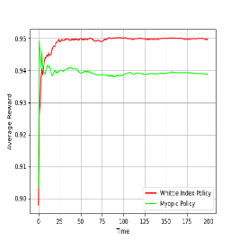
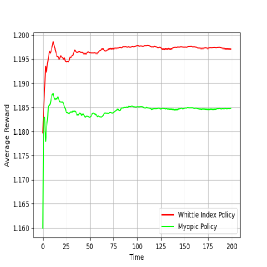
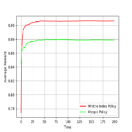
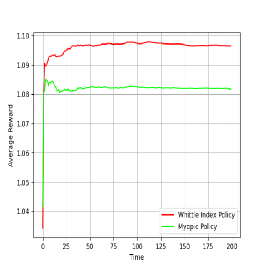
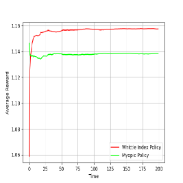
In the Whittle index algorithm, a small trouble is the calculation of approximate state space, which may spend more time in the case of higher dimensions. Therefore, in the actual numerical experiment, we mainly consider the three-state case. For the calculation of approxiamte state space, set the maximum number of iterations to 6, and the error limit $\varepsilon$ is $1e-3$. For each example, set the number of arms to 6, and the number of arms activated each time is 1, and other parameters are set to meet PCL indexability. We mainly consider the unit-time-return performance of Whittle index policy and myopic policy when the RMAB system runs for 200 time slots, using 10000 Monte Carlo simulation experiments. Figures 2-6 show that Whittle index policy has better performance than myopic policy (specific parameter settings are shown in Table 1-3).

Refer to caption
Figure 1: Example 1
Refer to caption
Figure 2: Example 2
Refer to caption
Figure 3: Example 3
Refer to caption
Figure 4: Example 4
Refer to caption
Figure 5: Example 5
Refer to caption
Figure 6: Example 6
Table 1: Transition Matrices Setting 1
Arm System 1 2 3
1 $\textbf{P}^{(1)}=\begin{pmatrix}0.524&0.221&0.255\\ 0.271&0.277&0.452\\ 0.337&0.281&0.382\end{pmatrix}$ $\textbf{P}^{(1)}=\begin{pmatrix}0.427&0.212&0.361\\ 0.305&0.320&0.375\\ 0.089&0.383&0.528\end{pmatrix}$ $\textbf{P}^{(1)}=\begin{pmatrix}0.305&0.333&0.362\\ 0.206&0.331&0.463\\ 0.236&0.179&0.585\end{pmatrix}$
2 $\textbf{P}^{(2)}=\begin{pmatrix}0.671&0.022&0.307\\ 0.396&0.215&0.389\\ 0.095&0.339&0.566\end{pmatrix}$ $\textbf{P}^{(2)}=\begin{pmatrix}0.504&0.172&0.324\\ 0.355&0.315&0.330\\ 0.129&0.303&0.568\end{pmatrix}$ $\textbf{P}^{(2)}=\begin{pmatrix}0.477&0.187&0.336\\ 0.391&0.266&0.343\\ 0.009&0.404&0.587\end{pmatrix}$
3 $\textbf{P}^{(3)}=\begin{pmatrix}0.371&0.237&0.392\\ 0.235&0.491&0.274\\ 0.443&0.154&0.403\end{pmatrix}$ $\textbf{P}^{(3)}=\begin{pmatrix}0.185&0.259&0.556\\ 0.160&0.595&0.245\\ 0.096&0.378&0.526\end{pmatrix}$ $\textbf{P}^{(3)}=\begin{pmatrix}0.255&0.356&0.389\\ 0.232&0.436&0.332\\ 0.175&0.083&0.742\end{pmatrix}$
4 $\textbf{P}^{(4)}=\begin{pmatrix}0.438&0.298&0.264\\ 0.413&0.460&0.127\\ 0.368&0.233&0.399\end{pmatrix}$ $\textbf{P}^{(4)}=\begin{pmatrix}0.575&0.279&0.146\\ 0.384&0.353&0.263\\ 0.068&0.201&0.731\end{pmatrix}$ $\textbf{P}^{(4)}=\begin{pmatrix}0.670&0.081&0.249\\ 0.712&0.102&0.186\\ 0.256&0.531&0.213\end{pmatrix}$
5 $\textbf{P}^{(5)}=\begin{pmatrix}0.610&0.229&0.161\\ 0.183&0.445&0.372\\ 0.565&0.162&0.273\end{pmatrix}$ $\textbf{P}^{(5)}=\begin{pmatrix}0.261&0.308&0.431\\ 0.215&0.709&0.076\\ 0.422&0.278&0.300\end{pmatrix}$ $\textbf{P}^{(5)}=\begin{pmatrix}0.394&0.085&0.521\\ 0.261&0.648&0.091\\ 0.467&0.133&0.400\end{pmatrix}$
6 $\textbf{P}^{(6)}=\begin{pmatrix}0.346&0.500&0.154\\ 0.392&0.414&0.194\\ 0.497&0.231&0.272\end{pmatrix}$ $\textbf{P}^{(6)}=\begin{pmatrix}0.301&0.436&0.263\\ 0.379&0.464&0.157\\ 0.372&0.152&0.476\end{pmatrix}$ $\textbf{P}^{(6)}=\begin{pmatrix}0.538&0.134&0.328\\ 0.700&0.117&0.183\\ 0.380&0.297&0.323\end{pmatrix}$
Table 2: Transition Matrices Setting 2
Arm System 4 5 6
1 $\textbf{P}^{(1)}=\begin{pmatrix}0.410&0.350&0.240\\ 0.412&0.403&0.185\\ 0.473&0.198&0.329\end{pmatrix}$ $\textbf{P}^{(1)}=\begin{pmatrix}0.586&0.261&0.153\\ 0.164&0.468&0.368\\ 0.018&0.395&0.587\end{pmatrix}$ $\textbf{P}^{(1)}=\begin{pmatrix}0.420&0.214&0.366\\ 0.317&0.338&0.345\\ 0.117&0.429&0.454\end{pmatrix}$
2 $\textbf{P}^{(2)}=\begin{pmatrix}0.524&0.221&0.255\\ 0.271&0.277&0.452\\ 0.337&0.281&0.382\end{pmatrix}$ $\textbf{P}^{(2)}=\begin{pmatrix}0.468&0.461&0.071\\ 0.457&0.448&0.095\\ 0.038&0.550&0.412\end{pmatrix}$ $\textbf{P}^{(2)}=\begin{pmatrix}0.285&0.362&0.353\\ 0.289&0.373&0.338\\ 0.037&0.378&0.585\end{pmatrix}$
3 $\textbf{P}^{(3)}=\begin{pmatrix}0.364&0.299&0.337\\ 0.346&0.480&0.174\\ 0.322&0.420&0.258\end{pmatrix}$ $\textbf{P}^{(3)}=\begin{pmatrix}0.263&0.392&0.345\\ 0.317&0.624&0.059\\ 0.247&0.565&0.188\end{pmatrix}$ $\textbf{P}^{(3)}=\begin{pmatrix}0.538&0.172&0.290\\ 0.379&0.468&0.153\\ 0.408&0.439&0.153\end{pmatrix}$
4 $\textbf{P}^{(4)}=\begin{pmatrix}0.383&0.601&0.016\\ 0.158&0.262&0.580\\ 0.537&0.393&0.070\end{pmatrix}$ $\textbf{P}^{(4)}=\begin{pmatrix}0.179&0.284&0.537\\ 0.322&0.674&0.004\\ 0.372&0.186&0.442\end{pmatrix}$ $\textbf{P}^{(4)}=\begin{pmatrix}0.286&0.581&0.133\\ 0.332&0.491&0.177\\ 0.406&0.352&0.242\end{pmatrix}$
5 $\textbf{P}^{(5)}=\begin{pmatrix}0.370&0.154&0.476\\ 0.440&0.178&0.382\\ 0.413&0.231&0.356\end{pmatrix}$ $\textbf{P}^{(5)}=\begin{pmatrix}0.419&0.253&0.328\\ 0.391&0.267&0.342\\ 0.202&0.393&0.405\end{pmatrix}$ $\textbf{P}^{(5)}=\begin{pmatrix}0.320&0.306&0.374\\ 0.341&0.381&0.278\\ 0.206&0.568&0.226\end{pmatrix}$
6 $\textbf{P}^{(6)}=\begin{pmatrix}0.262&0.432&0.306\\ 0.294&0.508&0.198\\ 0.250&0.339&0.411\end{pmatrix}$ $\textbf{P}^{(6)}=\begin{pmatrix}0.387&0.016&0.597\\ 0.270&0.283&0.447\\ 0.136&0.480&0.384\end{pmatrix}$ $\textbf{P}^{(6)}=\begin{pmatrix}0.163&0.102&0.735\\ 0.053&0.529&0.418\\ 0.121&0.435&0.444\end{pmatrix}$
Table 3: Error and Reward Matrix Setting
Error Matrix Reward Matrix
$\textbf{E}=\begin{pmatrix}0.90&0.05&0.05\\ 0.10&0.80&0.10\\ 0.10&0.05&0.85\end{pmatrix}$ $\textbf{R}=\begin{pmatrix}0&0&0\\ 0&1&0\\ 0&0&2\end{pmatrix}$
Note: the same error matrix and reward matrix were set for each arm in all experiments.

5 Conclusions

In this paper, we generalize the RMAB problem in the context of POMDP to the high-dimensional observation model, and construct the corresponding Whittle index policy. Starting from the rule of belief update in this case, we propose the concept of $T$-step belief state space and derive the transition probabilities between these states. When the number of states in the belief state space is large, the classic dynamic programming analysis for the RMAB problem suffers from the curse of dimensionality, so another method was applied. Based on achievable region and conservation law analysis studied in the literature for MAB problems, this paper first transforms the optimization problem into a linear programming one by defining performance measures for each state. For the problem of countable state space, under the condition of PCL indexability, it can be proven that with a loose regularity assumption, the two-arm problem also satisfies Whittle indexability, but a precise Whittle index algorithm for the countable state space is indeterminate. By introducing the concept of approximate state space, we convert the countable state space into a finite one, and calculate the approximate Whittle index of each state using a finite-state adaptive greedy algorithm. In Section 3 and 4, we summarize the complete Whittle index algorithm, and numerical simulation results show that the algorithm has significant improvements compared to the myopic policy.

Although we have quite a few theoretical analysis and confirmed the effectiveness of the approximate Whittle index algorithm with numerical experiments in this paper, there are still some problems to be solved in the future. An important problem is that the concept of approximate state space is proposed through a large number of numerical simulation experiments, and we have not yet proved Observation 1 and 2. Another problem is that we only analyzed the optimality of the Whittle index if the problem satisfies the PCL indexability with respect to some set family $\tilde{\Omega}$, but we have not been able to give the selection method of $\tilde{\Omega}$ and the exact algorithm for computing the Whittle index for the entire belief state space, so further rooms for exploration of problems with countable state spaces still await to be filled.

Declarations

  • Funding Not applicable

  • Conflict of interest/Competing interests Not applicable

  • Ethics approval Not applicable

  • Consent to participate Not applicable

  • Consent for publication Yes

  • Availability of data and materials Available upon request

  • Code availability Available upon request

  • Authors’ contributions Keqin Liu formulated the problem under the PCL framework and helped finish several key steps in theoretical proofs and the algorithm. Chengzhong Zhang completed the proofs, the algorithm and numerical simulations.

References

  • Ahmad et al. [2009] Ahmad, S. H. A., Liu, M., Javidi, T., Zhao, Q., and Krishnamachari, B. (2009). Optimality of myopic sensing in multichannel opportunistic access. IEEE Transactions on Information Theory, 55(9):4040–4050.
  • Anderson and Nash [1987] Anderson, E. J. and Nash, P. (1987). Linear programming in infinite-dimensional spaces: theory and applications. John Wiley & Sons.
  • Berry and Fristedt [1985] Berry, D. A. and Fristedt, B. (1985). Bandit problems: sequential allocation of experiments (monographs on statistics and applied probability). London: Chapman and Hall, 5(71-87):7–7.
  • Bertsimas [1995] Bertsimas, D. (1995). The achievable region method in the optimal control of queueing systems; formulations, bounds and policies. Queueing systems, 21:337–389.
  • Bertsimas and Niño-Mora [1996] Bertsimas, D. and Niño-Mora, J. (1996). Conservation laws, extended polymatroids and multiarmed bandit problems; a polyhedral approach to indexable systems. Mathematics of Operations Research, 21(2):257–306.
  • Bertsimas and Niño-Mora [2000] Bertsimas, D. and Niño-Mora, J. (2000). Restless bandits, linear programming relaxations, and a primal-dual index heuristic. Operations Research, 48(1):80–90.
  • Coffman and Mitrani [1980] Coffman Jr, E. G. and Mitrani, I. (1980). A characterization of waiting time performance realizable by single-server queues. Operations Research, 28(3-part-ii):810–821.
  • [8] Division, T. J. W. I. R. C. R. and Tsoucas, P. (1991). The region of achievable performance in a model of Klimov.
  • Farias and Madan [2011] Farias, V. F. and Madan, R. (2011). The irrevocable multiarmed bandit problem. Operations Research, 59(2):383–399.
  • Federgruen and Groenevelt [1988] Federgruen, A. and Groenevelt, H. (1988a). Characterization and optimization of achievable performance in general queueing systems. Operations Research, 36(5):733–741.
  • Federgruen and Groenevelt [1988] Federgruen, A. and Groenevelt, H. (1988b). M/g/c queueing systems with multiple customer classes: Characterization and control of achievable performance under nonpreemptive priority rules. Management Science, 34(9):1121–1138.
  • Frostig and Weiss [1999] Frostig, E. and Weiss, G. (1999). Four proofs of gittins’ multiarmed bandit theorem. Applied Probability Trust, 70:427.
  • Gelenbe and Mitrani [2010] Gelenbe, E. and Mitrani, I. (2010). Analysis and synthesis of computer systems, volume 4. World Scientific.
  • Gittins et al. [2011] Gittins, J., Glazebrook, K., and Weber, R. (2011). Multi-armed bandit allocation indices. John Wiley & Sons.
  • Gittins [1979] Gittins, J. C. (1979). Bandit processes and dynamic allocation indices. Journal of the Royal Statistical Society: Series B (Methodological), 41(2):148–164.
  • Glazebrook et al. [2002] Glazebrook, K., Nino-Mora, J., and Ansell, P. (2002). Index policies for a class of discounted restless bandits. Advances in Applied Probability, 34(4):754–774.
  • Hoffman et al. [2011] Hoffman, M., Brochu, E., De Freitas, N., et al. (2011). Portfolio allocation for bayesian optimization. In UAI, pages 327–336.
  • Klimov [1975] Klimov, G. P. (1975). Time-sharing service systems. i. Theory of Probability & Its Applications, 19(3):532–551.
  • Liu [2021] Liu, K. (2021). Index policy for a class of partially observable markov decision processes. arXiv preprint arXiv:2107.11939.
  • Liu et al. [2011] Liu, K., Weber, R., and Zhao, Q. (2011). Indexability and whittle index for restless bandit problems involving reset processes. In 2011 50th IEEE Conference on Decision and Control and European Control Conference, pages 7690–7696. IEEE.
  • Liu and Zhao [2010] Liu, K. and Zhao, Q. (2010). Indexability of restless bandit problems and optimality of whittle index for dynamic multichannel access. IEEE Transactions on Information Theory, 56(11):5547–5567.
  • Liu et al. [2010] Liu, K., Zhao, Q., and Krishnamachari, B. (2010). Dynamic multichannel access with imperfect channel state detection. IEEE Transactions on Signal Processing, 58(5):2795–2808.
  • Niño-Mora [2001] Niño-Mora, J. (2001). Restless bandits, partial conservation laws and indexability. Advances in Applied Probability, 33(1):76–98.
  • Niño-Mora [2002] Niño-Mora, J. (2002). Dynamic allocation indices for restless projects and queueing admission control: a polyhedral approach. Mathematical programming, 93(3):361–413.
  • Niño-Mora [2006] Niño-Mora, J. (2006). Restless bandit marginal productivity indices, diminishing returns, and optimal control of make-to-order/make-to-stock m/g/1 queues. Mathematics of Operations Research, 31(1):50–84.
  • Niño-Mora [2007] Niño-Mora, J. (2007). Dynamic priority allocation via restless bandit marginal productivity indices. Top, 15(2):161–198.
  • Papadimitriou and Tsitsiklis [1994] Papadimitriou, C. H. and Tsitsiklis, J. N. (1994). The complexity of optimal queueing network control. In Proceedings of IEEE 9th Annual Conference on Structure in Complexity Theory, pages 318–322. IEEE.
  • Press [2009] Press, W. H. (2009). Bandit solutions provide unified ethical models for randomized clinical trials and comparative effectiveness research. Proceedings of the National Academy of Sciences, 106(52):22387–22392.
  • Robbins [1952] Robbins, H. (1952). Some aspects of the sequential design of experiments.
  • Rudin et al. [1976] Rudin, W. et al. (1976). Principles of mathematical analysis, volume 3. McGraw-hill New York.
  • Shen et al. [2015] Shen, W., Wang, J., Jiang, Y.-G., and Zha, H. (2015). Portfolio choices with orthogonal bandit learning. In Twenty-fourth international joint conference on artificial intelligence.
  • Smallwood and Sondik [1973] Smallwood, R. D. and Sondik, E. J. (1973). The optimal control of partially observable markov processes over a finite horizon. Operations research, 21(5):1071–1088.
  • Sondik [1978] Sondik, E. J. (1978). The optimal control of partially observable markov processes over the infinite horizon: Discounted costs. Operations research, 26(2):282–304.
  • Weber and Weiss [1990] Weber, R. R. and Weiss, G. (1990). On an index policy for restless bandits. Journal of applied probability, 27(3):637–648.
  • Whittle [1988] Whittle, P. (1988). Restless bandits: Activity allocation in a changing world. Journal of applied probability, 25(A):287–298.
  • Zhao and Sadler [2007] Zhao, Q. and Sadler, B. M. (2007). A survey of dynamic spectrum access. IEEE signal processing magazine, 24(3):79–89.