Biorthogonal dynamical quantum phase transitions in non-Hermitian systems

Abstract

By using biorthogonal bases, we construct a complete framework for biorthogonal dynamical quantum phase transitions in non-Hermitian systems. With the help of associated state which is overlooked previously, we define the automatically normalized biorthogonal Loschmidt echo. This approach is capable of handling arbitrary non-Hermitian systems with complex eigenvalues, which naturally eliminates the negative value of Loschmidt rate obtained without the biorthogonal bases. Taking the non-Hermitian Su-Schrieffer-Heeger model as a concrete example, a peculiar $1/2$ change in biorthogonal dynamical topological order parameter, which is beyond the traditional dynamical quantum phase transitions is observed. We also find the periodicity of biorthogonal dynamical quantum phase transitions depend on whether the two-level subsystem at the critical momentum oscillates or reaches a steady state.

The past decades have witnessed the flourishing of non-Hermitian physics in non-conservative systems as found in a variety of physical realms including open quantum systems Rotter2009JPA , electronic systems with interactions Yoshida2018PRB ; Shen2018PRL ; Fu2020PRL , and classical systems with gain or loss Makris2008PRL ; Klaiman2008PRL ; Malzard2015PRL . In these systems Bender1998PRL ; Helbig2020NatPhys ; Liu2021Research ; Weidemann2020Science ; Brandenbourger2019NatCommun ; Ghatak2020PNAS ; XZhang2021NatCommun ; LZhang2021NatCommun ; Xiao2020NatPhys ; Wang2021JOpt ; ZhongWang2018PRL ; Sato2019PRX ; Yokomizo2019PRL ; Shen2018PRL2 , many novel physics and unprecedented phenomena have been explored recently, such as the exceptional points Hodaei2017Nature ; Bergholtz2021RMP , the non-Hermitian skin effects Zhang2020PRL ; XiujuanZhang2022AdvPX , the bulk Fermi arcs Zhou2018Science , and so on. In contrast to the Hermitian systems with real eigenvalues and orthogonal eigenstates, the eigenvalues and eigenstates in a general non-Hermitian Hamiltonian are not necessarily real and orthogonal Ueda2020AdvPhys . To be more precise, the orthogonality of eigenstates is replaced by the notion of biorthogonality that defines the relation between the Hilbert space of states and its dual space, leading to the so-called “biorthogonal quantum mechanics” Brody2014JPA ; Emil2018PRL ; Emil2019PRBR ; Emil2020PRR . A direct consequence of the biorthogonality is that the transition probability between one state $\left|\phi\right\rangle$ to its time-evolved state $\left|\phi\left(t\right)\right\rangle$ should be carefully defined. The traditional viewpoint $p=\left|\left\langle\phi\left(t\right)|\phi\right\rangle\right|^{2}$ used in Hermitian systems cannot be applied to a general non-Hermitian Hamiltonian. A schematic framework to deal with this becomes an urgent topic due to the rapid development of nonequilibrium studys in non-Hermitian systems ShuChen2021PRA ; HuiZhai2020NatPhys ; Lin2022NPJQI ; Liu2023PRA ; Hauke2022PRXQ ; Kawabata2023PRX ; Yoshimura2020PRB ; Mcdonald2022PRB ; Yin2022PRB ; Agarwal2022arXiv ; Agarwal2023arXiv ; Roubeas2023JHEP .

Dynamical quantum phase transition (DQPT) is arguably one of the most important nonequilibrium phenomena in modern many-body physics and has also been extensively studied in past decades Heyl2013PRL ; Budich2016PRB ; Dong2019PRB ; Nie2020PRL ; ShuChen2023PRB . It was first introduced in the Hermitian transverse field Ising model Heyl2013PRL and was generalized to mixed state Heyl2017PRB ; Bhattacharya2017PRB , finite temperature Abeling2016PRB ; Sedlmayr2018PRB ; Halimeh2018PRL ; Halimeh2018PRB , Floquet systems Yang2019PRB ; Naji2022PRA ; Jafari2021PRA ; Jafari2022PRB , and slow quench process Sharma2016PRB . It was also observed experimentally with trapped ions Shen2017PRL ; Zhang2017Nature , Rydberg atoms Bernien2017Nature , ultracold atoms Sengstock2018NatPhys , superconducting qubits HengFan2019PRAppl , nanomechanical and photonic systems JiangfengDu2019PRB ; PengXue2019PRL ; GuangcanGuo2020LSA . The key quantity characterizing DQPT is the Loschmidt echo or dynamical fidelity, $\mathcal{L}\left(t\right)\equiv\left|\left\langle\Psi\left(0\right)|\Psi\left(t\right)\right\rangle\right|^{2}$, quantifying the time-dependent deviation from an arbitrary initial state $\left|\Psi\left(0\right)\right\rangle$. In Hermitian systems, DQPTs occur whenever the time-evolved state $\left|\Psi\left(t\right)\right\rangle$ becomes orthogonal to the initial state $\left|\Psi\left(0\right)\right\rangle$ and the critical time $t_{c}$ is defined as $\mathcal{L}\left(t_{c}\right)=0$. Efforts have been made to generalize this concept to non-Hermitian systems, leading to many interesting predictions such as the half-integer jumps in dynamical topological order parameter (DTOP) Mondal2022PRB , but the special biorthogonality has been ignored and an enforced normalized factor has been used Zhou2018PRA ; Zhou2021NJP ; Mondal2022arxiv . Very recently, it has been shown that the non-Hermitian systems should be described by the biorthogonal fidelity and the biorthogonal Loschmidt echo instead of the conventional counterparts in Hermitian systems, but it is limited to the parity-time symmetry cases Sun2022FP ; Tang2022EPL . A natural treatment for a general non-Hermitian Hamiltonian is still lacking, which severely limits our exploration of the richness of DQPTs in these systems.

In this work, we address this issue by proposing a new theoretical framework to deal with these non-equilibrium phenomena in general non-Hermitian systems. Based on biorthogonal quantum mechanics, we reformulate the transition probability between $\left|\Psi\left(0\right)\right\rangle$ and $\left|\Psi\left(t\right)\right\rangle$ with the biorthogonal bases and the associated states. We propose the biorthogonal dynamical quantum phase transitions and compare it with the self-normal counterpart using the non-Hermitian Su-Schrieffer-Heeger model as a concrete example. We systematically study the biorthogonal Loschmidt rate, biorthogonal DTOP, Fisher zeros and the transition probability in momentum space when the system undergoes a sudden quench. Our calculations show that there is a peculiar half-jump in biorthogonal DTOP and the periodicity of biorthogonal DQPTs depend on whether the two-level subsystem at the critical momentum oscillates or reaches a steady state. Our theory provides a general scheme to study the non-equilibrium DQPTs in non-Hermitian systems.

We first review some basic properties of biorthogonal quantum mechanics in non-Hermitian systems and reformulate the probability assignment rules between two states with biorthogonal bases Brody2014JPA . For a general non-Hermitian Hamiltonian $H\neq H^{{\dagger}}$, the eigenvalue equations of $H$ and $H^{{\dagger}}$ are given by

$$H|u_{n}\rangle =\epsilon_{n}|u_{n}\rangle,\quad\langle u_{n}|H^{\dagger}=\epsilon_{n}^{\ast}\langle u_{n}|,$$

$$H^{{\dagger}}\left|\widetilde{u}_{n}\right\rangle =\epsilon_{n}^{\ast}\left|\widetilde{u}_{n}\right\rangle,\quad\left\langle\widetilde{u}_{n}\right|H=\epsilon_{n}\left\langle\widetilde{u}_{n}\right|,$$ (1)

where $\epsilon_{n}$ is the nth eigenvalue, $|u_{n}\rangle$ and $\left|\widetilde{u}_{n}\right\rangle$ are the right and left eigenstates that satisfy the completeness relation $\sum_{n}|\widetilde{u}_{n}\rangle\langle u_{n}|=1$ and the biorthonormal relation $\langle\widetilde{u}_{m}|u_{n}\rangle=\delta_{m,n}$. Note that under this condition $\langle\widetilde{u}_{n}|u_{n}\rangle=1$, eigenstates are no longer be normalized. In particular, we have $\langle u_{n}|u_{n}\rangle\geq 1$ and $\langle u_{n}|u_{m}\rangle\neq 0$ if $n\neq m$. It challenges the traditional probabilistic interpretation used in Hermitian quantum mechanics. For instance, there cannot be a ‘transition’ from one eigenstate $|u_{m}\rangle$ to another eigenstate $|u_{n}\rangle$ due to the orthonormal relation $\langle u_{n}|u_{m}\rangle=0$ if $n\neq m$ in Hermitian systems. To reconcile these apparent contradictions we need the introduction of the so-called associated state and the redefinition of the inner product. For an arbitrary state $|\psi\rangle$, its associated state $|\widetilde{\psi}\rangle$ is defined according to the following relation Brody2014JPA :

$$|\psi\rangle=\sum_{n}c_{n}|u_{n}\rangle\longleftrightarrow|\widetilde{\psi}\rangle=\sum_{n}c_{n}|\widetilde{u}_{n}\rangle.$$ (2)

While the dual state $\langle\widetilde{\psi}|=\sum_{n}c_{n}^{\ast}\left\langle\widetilde{u}_{n}\right|$ is given by the Hermitian conjugate of $|\widetilde{\psi}\rangle$. The inner product between $|\psi\rangle$ and another state $|\phi\rangle=\sum_{m}d_{m}|u_{m}\rangle$ is thus defined as

$$\langle\phi,\psi\rangle\equiv\langle\widetilde{\phi}|\psi\rangle=\sum_{m,n}\langle\widetilde{u}_{m}|d_{m}^{\ast}c_{n}|u_{n}\rangle=\sum_{n}d_{n}^{\ast}c_{n}.$$ (3)

It is easy to show that the norm of a state $|\psi\rangle$ is $\sqrt{\langle\widetilde{\psi}|\psi\rangle}$. With these new definitions, the transition probability between $|\psi\rangle$ and $|\phi\rangle$ for a biorthogonal system is given by

$$p=\frac{\langle\widetilde{\psi}|\phi\rangle\langle\widetilde{\phi}|\psi\rangle}{\langle\widetilde{\psi}|\psi\rangle\langle\widetilde{\phi}|\phi\rangle},$$ (4)

where the denominator acts as a natural normalizing factor. In this case, $p$ is a real number ranging from $0$ to $1$, which meets the requirements of probability interpretation satisfactorily. If the Hamiltonian is Hermitian $H=H^{{\dagger}}$, we have $|\widetilde{u}_{n}\rangle=|u_{n}\rangle$ and $|\widetilde{\psi}\rangle=|\psi\rangle$. Then Eq. (4) reduces to the conventional definition of the transition probability in Hermitian quantum mechanics $p=\langle\psi|\phi\rangle\langle\phi|\psi\rangle/\left(\langle\psi|\psi\rangle\langle\phi|\phi\rangle\right)$. Another important consequence of Eq. (4) is that the projection from $|\psi\rangle=\sum_{n}c_{n}|u_{n}\rangle$ to $|u_{n}\rangle$ becomes

$$p_{n}=\frac{\langle\widetilde{\psi}|u_{n}\rangle\langle\widetilde{u}_{n}|\psi\rangle}{\langle\widetilde{\psi}|\psi\rangle\langle\widetilde{u}_{n}|u_{n}\rangle}=\frac{c_{n}^{\ast}c_{n}}{\sum_{m}c_{m}^{\ast}c_{m}},$$ (5)

satisfying the normalization condition $\sum_{n}p_{n}=1$.

So far we have considered the static aspects of the eigenvalues and eigenstates of a complex Hamiltonian. The generalization to dynamical situation is straightforward. The time evolution of an initial state $|\Psi\left(0\right)\rangle$ generated by an arbitrary non-Hermitian Hamiltonian $H$ is $|\Psi\left(t\right)\rangle=\operatorname{e}^{-\operatorname*{i}Ht}\left|\Psi\left(0\right)\right\rangle$ where we have assumed a time-independent Hamiltonian for simplicity. It’s worth noting that the associated state $|\widetilde{\Psi}\left(t\right)\rangle$ should be given by definition Eq. (2) Brody2014JPA rather than $|\widetilde{\Psi}\left(t\right)\rangle=\operatorname{e}^{-\operatorname*{i}H^{{\dagger}}t}|\widetilde{\Psi}\left(0\right)\rangle$ Yoshimura2020PRB because the second method may lead to an incomprehensible complex probabilities (Appendix A). The overlap between $|\Psi\left(0\right)\rangle$ and $|\Psi\left(t\right)\rangle$ is characterized by the biorthogonal Loschmidt echo,

$$\mathcal{L}\left(t\right)=\frac{\langle\widetilde{\Psi}\left(0\right)|\Psi\left(t\right)\rangle\langle\widetilde{\Psi}\left(t\right)|\Psi\left(0\right)\rangle}{\langle\widetilde{\Psi}\left(t\right)|\Psi\left(t\right)\rangle\langle\widetilde{\Psi}\left(0\right)|\Psi\left(0\right)\rangle}.$$ (6)

As in Hermitian case, the biorthogonal DQPTs can be defined as $\mathcal{L}\left(t_{c}\right)=0$ with the critical time $t_{c}$.

We may examine the biorthogonal DQPT by considering a general non-Hermitian Hamiltonian $H=\sum_{k}\psi_{k}^{{\dagger}}H_{k}\psi_{k}$ with $H_{k}=\bm{d}_{k}\cdot\bm{\sigma}$. Here, $\bm{\sigma}$ is the vector of the Pauli matrices and $\bm{d}_{k}=\left(x_{k},y_{k},z_{k}\right)$ represent the expansion coefficients which may be complex in non-Hermitian systems. The eigenenergies of $H_{k}$ are given by $\pm\epsilon_{k}=\pm\sqrt{|\bm{d}_{k}|^{2}}$ and the corresponding eigenstates are $|u_{k\pm}\rangle$. Considering a quench process where the model Hamiltonian changes from $\bm{d}_{k}^{i}$ at time $t=0^{-}$ to $\bm{d}_{k}^{f}$ at time $t=0^{+}$, the initial state $|\Psi\left(0\right)\rangle={\textstyle\bigotimes\nolimits_{k}}|u_{k-}^{i}\rangle$ which is defined as the tensor product of all $|u_{k-}^{i}\rangle$ is evolved under the postquench Hamiltonian $\bm{d}_{k}^{f}$. The biorthogonal Loschmidt echo can be expressed as $\mathcal{L}(t)=\prod_{k}g_{k}(t)$ with (Appendix B)

$$g_{k}(t)=\frac{|\cos(\epsilon_{k}^{f}t)-\operatorname*{i}\sin(\epsilon_{k}^{f}t)\langle\widetilde{u}_{k-}^{i}|\frac{H_{k}^{f}}{\epsilon_{k}^{f}}|u_{k-}^{i}\rangle|^{2}}{\langle\widetilde{u}_{k-}^{i}(t)|u_{k-}^{i}(t)\rangle},$$ (7)

where $|u_{k-}^{i}(t)\rangle=\text{e}^{-\operatorname*{i}H^{f}_{k}t}|u_{k-}^{i}\rangle$. To obtain a nonzero and well-defined quantity in the thermodynamic limit it is useful to consider the biorthogonal Loschmidt rate

$$\text{LR}(t) =-\displaystyle\lim_{N\to\infty}\frac{1}{N}\ln{\mathcal{L}(t)},$$ (8)

where $N$ is the system size. Zeros in $\mathcal{L}(t)$ at critical times $t_{c}$ correspond to nonanalyticities (cusps or divergencies) in $\text{LR}(t)$. If there is at least one pair of critical parameters $k_{c}$ and $t_{c}$ such that $g_{k_{c}}(t_{c})=0$, then $\mathcal{L}(t_{c})=0$. The solution of $g_{k_{c}}(t_{c})=0$ is

$$t_{c}=\frac{\pi}{2\epsilon^{f}_{k_{c}}}(2n+1)-\frac{\operatorname*{i}}{\epsilon^{f}_{k_{c}}}\tanh^{-1}\langle\widetilde{u}_{k_{c}-}^{i}|\frac{H_{k_{c}}^{f}}{\epsilon_{k_{c}}^{f}}|u_{{k}_{c}-}^{i}\rangle,$$ (9)

where $n$ is an integer. If we can obtain a positive real solution $t_{c}$, the system will undergo a biorthogonal DQPT. In general, it is difficult to access $k_{c}$ in a finite-size system because momentum takes quantized values. Thus the divergence of $\text{LR}(t)$ in the thermodynamic limit becomes a cusp in a finite-site system except for some fine-tuned quench parameters or twist boundary conditions ShuChen2023PRB . Furthermore, analogous to DTOP in Hermitian systems Vajna2015PRB , we can propose a biorthogonal DTOP to describe biorthogonal DQPT. The biorthogonal DTOP is defined as

$$\nu(t)=\frac{1}{2\pi}\int_{0}^{2\pi}dk\partial_{k}\phi_{k}^{G}(t),$$ (10)

where the biorthogonal geometrical phase is $\phi^{G}_{k}(t)=\phi_{k}(t)-\phi_{k}^{\text{dyn}}(t)$, with $\phi_{k}(t)$ being the phase of $g_{k}(t)$ and the biorthogonal dynamical phase is given by (Appendix B)

$$\phi_{k}^{\text{dyn}}(t)= -\int_{0}^{t}ds\frac{\langle\widetilde{u}_{k-}^{i}(s)|H_{k}^{f}|u_{k-}^{i}(s)\rangle}{\langle\widetilde{u}_{k-}^{i}(s)|u_{k-}^{i}(s)\rangle}$$

$$+\frac{\text{i}}{2}\text{ln}\langle\widetilde{u}_{k-}^{i}(t)|u_{k-}^{i}(t)\rangle.$$ (11)

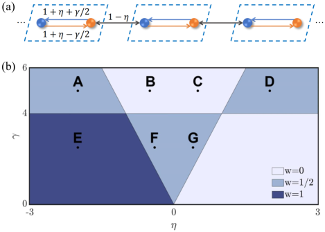
Figure 1: (a) The sketch of non-Hermitian Su-Schrieffer-Heeger model. The box indicates the unit cell. (b) The $\gamma$-$\eta$ phase diagram. Each region filled with a different color corresponds to a phase with a topological winding number $w$. The boundaries between the regions are determined using $\epsilon_{k}=0$. The black points represent different parameters ($\eta$, $\gamma$) which will be used below. Specifically, the points A to G represent (-2, 5), (-0.2, 5), (0.2, 5), (2, 5), (-2, 1), (-0.2, 1), and (0.2, 1), respectively.

To demonstrate that our new theoretical framework can successfully deal with non-Hermitian Hamiltonians with complex eigenvalues, we study the non-Hermitian Su-Schrieffer-Heeger model in detail below. The Hamiltonian is

$$H =\sum_{j}\left[\left(1+\eta+\frac{\gamma}{2}\right)c_{j,b}^{{\dagger}}c_{j,a}+\left(1+\eta-\frac{\gamma}{2}\right)c_{j,a}^{{\dagger}}c_{j,b}\right.$$

$$\left.\quad+\left(1-\eta\right)c_{j,a}^{{\dagger}}c_{j+1,b}+\left(1-\eta\right)c_{j+1,b}^{{\dagger}}c_{j,a}\right],$$ (12)

where $\eta$ determines the strength of intra-cell and inter-cell hopping and $\gamma$ controls the degree of non-Hermiticity, as shown in Fig. 1(a). For periodic boundary condition, the bulk Hamiltonian gets the standard bilinear form $H=\sum_{k}\psi_{k}^{\dagger}\left(\bm{d}_{k}\cdot\bm{\sigma}\right)\psi_{k}$ in momentum space, where $\psi_{k}^{\dagger}=(c_{k,a}^{{\dagger}},c_{k,b}^{{\dagger}})$ and

$$\bm{d}_{k}=\left(\left(1+\eta\right)+\left(1-\eta\right)\cos k,\left(1-\eta\right)\sin k+\operatorname*{i}\frac{\gamma}{2},0\right).$$ (13)

The dispersion is $\pm\epsilon_{k}=\pm\sqrt{x_{k}^{2}+y_{k}^{2}}$. It becomes gapless at the exceptional points. Thus the solution of $\epsilon_{k}=0$ determines the phase boundary, i.e. $k_{c}=0,\;\gamma=\pm 4$ and $k_{c}=\pi,\;\gamma=\pm 4\eta$. Combining with the winding number $w=\frac{1}{2\pi}\int_{0}^{2\pi}dk\partial_{k}\left(\arctan\frac{y_{k}}{x_{k}}\right)$ Yin2018PRA , we present the phase diagram in Fig. 1(b) for convenience, where we only consider the case $\gamma>0$ due to the symmetry of the phase diagram with respect to $\gamma$.

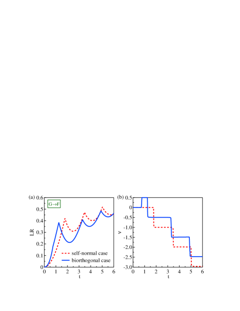
Figure 2: (a) The Loschmidt rate and (b) the DTOP with self-normal and biorthogonal bases for a typical quench process (from G to F).

For comparison, we also calculate the traditional DQPT based on self-normal Loschmidt echo $\mathcal{L}\left(t\right)=\left|\left\langle\Psi\left(0\right)|\Psi\left(t\right)\right\rangle\right|^{2}$, with an enforced normalized factor to avoid the negative value of Loschmidt rate Zhou2018PRA . Figure 2(a) presents the self-normal and biorthogonal Loschmidt rate from the same quenching process. The first feature is that the critical time at which the cusp appears is different from each other. A similar phenomenon has been observed in equilibrium quantum phase transitions, where the biorthogonal and self-normal fidelity predict different quantum critical points Sun2022FP . It turns out that the biorthogonal fidelity captures the correct critical point due to the special biorthoganality in non-Hermitian systems Sun2022FP . Thus it is also nature to believe that the non-equilibrium quantum phase transitions should be described by the biorthogonal time-dependent version of the fidelity, i.e. biorthogonal Loschmidt echo. The second feature is that there is an additional critical time $t_{c}\approx 0.74$ in biorthogonal bases. This can be seen more clearly in the DTOP as shown in Fig. 2(b). A peculiar half-jump of $\nu(t)$ can be observed and it may be related to the biorthoganality.

To show that the half jump of $\nu(t)$ is not a fine-tune result Ding2020PRBR , we study different quenching processes by changing $\eta$ but with $\gamma$ fixed. Figures 3(a) and 3(b) presents five typical behaviour of the biorthogonal Loschmidt rate $\text{LR}\left(t\right)$ and biorthogonal DTOP $\nu(t)$, respectively. And more detailed information can be found in Appendix C. The half jump of $\nu(t)$ can appear alone, periodically or accompany by an integer jump, exhibiting rich behavior in a single non-Hermitian Hamiltonian. We also find that the half-jump phenomenon occurs if and only if the prequench phases are in the middle of the phase diagram with 0 or 1/2 winding number.

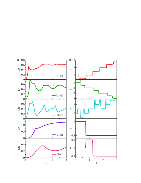
Figure 3: Five different types of quench processes showing a $\frac{1}{2}$ change in the biorthogonal DTOP. (a) and (b) illustrate the biorthogonal Loschmidt rate and biorthogonal DTOP, respectively. The $\frac{1}{2}$ change in the biorthogonal DTOP appears if and only if the prequench phases are in the middle of the phase diagram, with winding numbers of $\frac{1}{2}$ or $0$.

To better understand the biorthogonal DQPTs, we study the dynamical counterpart of Fisher zeros Fisher1967RPP ; Yang1952PR ; Lee1952PR in the complex time plane $z_{n}(k)=\text{i}t_{n}(k)$. The lines $z_{n}(k)$ cross the imaginary time axis at a critical momentum $k_{c}$ and yields a critical time $t_{c,n}$, as shown in Figs. 4(a) and 4(b). In fact, they represent two typical types of biorthogonal DQPTs, depending on whether the lines $z_{n}(k)$ cut the time axis periodically or non-periodically. In order to further study these two types of biorthogonal DQPTs, we also investigate the transition probability $p(k,t)$ between the time-evolved state $|u_{k-}^{i}(t)\rangle=\text{e}^{-\text{i}H^{f}_{k}t}|u_{k-}^{i}\rangle$ and another initial eigenstate $|u_{k+}^{i}\rangle$. By expanding $|u_{k-}^{i}(t)\rangle$ as $|u_{k-}^{i}(t)\rangle=c_{1}|u_{k-}^{i}\rangle+c_{2}|u_{k+}^{i}\rangle$, we have $p(k,t)=c_{1}^{\ast}c_{1}/(c_{1}^{\ast}c_{1}+c_{2}^{\ast}c_{2})$ from Eq. (5). If there exists $p(k,t)=1$, the time-evolved state $|u_{k-}^{i}(t)\rangle$ is biorthogonal with $|u_{k-}^{i}\rangle$. Then the biorthogonal Loschmidt echo equals to zero because we can rewrite $\mathcal{L}(t)$ as

$$\mathcal{L}(t)=\prod_{k}\frac{\langle\widetilde{u}_{k-}^{i}|u_{k-}^{i}(t)\rangle\langle\widetilde{u}_{k-}^{i}(t)|u_{k-}^{i}\rangle}{\langle\widetilde{u}_{k-}^{i}(t)|u_{k-}^{i}(t)\rangle}.$$ (14)

As shown in Figs. 4(c) and 4(d), the two types of biorthogonal DQPTs exhibit two distinct behaviour of $p(k,t)$. For the periodic biorthogonal DQPTs, $p(k_{c},t)$ oscillate periodically between $0$ and $1$ for some fixed critical momenta $k_{c}$. In this situation, the two-level systems of $k_{c}$ dominate. Thus the periodicity of biorthogonal DQPTs may be related to the oscillations of two-level system Zakrzewski2022arXiv . On the other hand, $p(k_{c},t)$ exhibit very interesting behavior when the biorthogonal DQPTs are no longer periodic. There are many critical momenta $k_{c}$ and each $k_{c}$ corresponds to only one $t_{c,n}$. Before $t_{c,n}=-\text{i}z_{n}(k_{c})$, there are $n$ local maximum in $p(k_{c},t)$. While for $t\gg t_{c,n}$, $p(k_{c},t)$ tends to a fixed value, indicating a steady state in contrast to the oscillation behaviour.

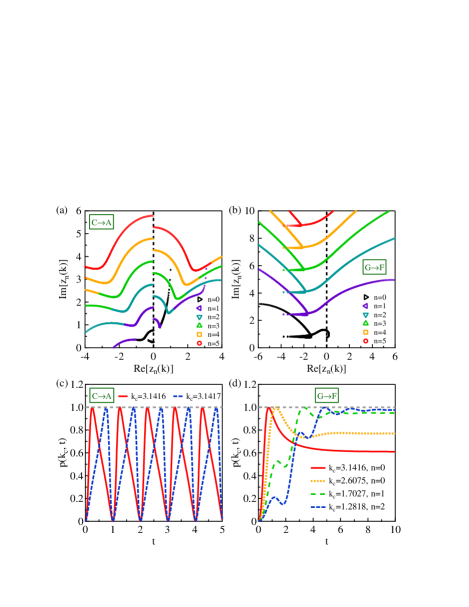
Figure 4: (a), (b) The dynamical Fisher zeros in the complex plane $z_{n}(k)=\text{i}t_{n}(k)$ with $k$ lies in the first Brillouin zone for two typical quench processes. (c), (d) The corresponding transition probability $p(k_{c},t)$ between $|u_{k_{c}-}^{i}(t)\rangle$ and $|u_{k_{c}+}^{i}\rangle$ at the critical momentum $k_{c}$.

In summary, we propose a new theoretical framework to study the biorthogonal DQPTs in non-Hermitian systems based on the biorthogonal quantum mechanics. We reformulate the transition probability between one state $\left|\Psi\left(0\right)\right\rangle$ and its time-evolved state $\left|\Psi\left(t\right)\right\rangle$ with the concept of associated state. Our scheme can handle general non-Hermitian Hamiltonian with complex eigenvalues and the normalization factors can be introduced naturally. We demonstrate our approach using the non-Hermitian Su-Schrieffer-Heeger model as a concrete example. Comparing with the self-normal cases, an peculiar 1/2 change in the biorthogonal DTOP can be observed clearly. Furthermore, our results show that the periodicity of biorthogonal DQPTs depend on whether the two-level subsystem at the critical momentum oscillates or reaches a steady state. Our work paves a way to explore the rich biorthogonal DQPTs in non-Hermitian systems. One interesting topic along this line would be the study of the mechanism of the 1/2 change in the biorthogonal DTOP.

Appendix A A simple example to illustrate the associate state

Here, we effectively demonstrate distinctions between various treatment methods by utilizing concrete $2\times 2$ non-Hermitian matrices that contain complex eigenvalues. In a simple example, we use the matrices

$$H=\left(\begin{matrix}0&4+\text{i}\\ 2-\text{i}&0\end{matrix}\right),$$ (15)

with biorthogonal bases

$$|\psi_{\pm}\rangle=\frac{1}{\sqrt{2}}\left(\begin{matrix}\pm\sqrt{\frac{4+\text{i}}{2-\text{i}}}\\ 1\end{matrix}\right),\;|\widetilde{\psi}_{\pm}\rangle=\frac{1}{\sqrt{2}}\left(\begin{matrix}\pm\sqrt{\frac{2+\text{i}}{4-\text{i}}}\\ 1\end{matrix}\right),$$ (16)

and

$$K=\left(\begin{matrix}0&-3\text{i}\\ -2+3\text{i}&0\end{matrix}\right)$$ (17)

for the time evolution.

Two methods can be employed to determine its associated state: treatment Eq. (2) with the time-evolved state $|\psi_{+}(t)\rangle=\text{e}^{-\operatorname*{i}Kt}|\psi_{+}\rangle$ denoted by subscript $1$ and treatment $|\widetilde{\psi}_{+}(t)\rangle=\text{e}^{-\operatorname*{i}K^{\dagger}t}|\widetilde{\psi}_{+}\rangle$ denoted by subscript $2$. When $t=1$, these methods lead to distinct states as represented by the following equations

$$|\widetilde{\psi}_{+}(t)\rangle_{1} =\left(\begin{matrix}-0.614+0.103\operatorname*{i}\\ -0.359-0.927\operatorname*{i}\end{matrix}\right),$$

$$|\widetilde{\psi}_{+}(t)\rangle_{2} =\left(\begin{matrix}-0.967-1.094\operatorname*{i}\\ -1.373+0.411\operatorname*{i}\end{matrix}\right).$$ (18)

To demonstrate why the second approach fails for Hamiltonians with complex eigenvalues, we calculate probabilities when transitioning from the state $|\psi_{+}(t)\rangle$ to an arbitrary state, for instance, $|\phi\rangle=2|\psi_{+}\rangle+3|\psi_{-}\rangle$, whose associated state is given by $|\widetilde{\phi}\rangle=2|\widetilde{\psi}_{+}\rangle+3|\widetilde{\psi}_{-}\rangle$. By utilizing two methods above to obtain the associated states in Eq. (18) and then applying Eq. (4) to calculate the transition probabilities, two different probabilities $p_{1}=0.603$ and $p_{2}=-0.372+1.118\operatorname*{i}$ are obtained. As shown above, the former is a real value while the latter is an incomprehensible complex result. Thus our treatment reaches a real valued probability between $0$ and $1$.

Appendix B Detail calculations of Eq. (7) and Eq. (11)

We can rewrite the biorthogonal Loschmidt echo as

$$\mathcal{L}(t) =\frac{|\langle\widetilde{\Psi}(0)|\Psi(t)\rangle|^{2}}{\langle\widetilde{\Psi}(t)|\Psi(t)\rangle\langle\widetilde{\Psi}(0)|\Psi(0)\rangle}$$

$$=\prod_{k}\frac{|\langle\widetilde{u}_{k-}^{i}|u_{k-}^{i}(t)\rangle|^{2}}{\langle\widetilde{u}_{k-}^{i}(t)|u_{k-}^{i}(t)\rangle\langle\widetilde{u}_{k-}^{i}|u_{k-}^{i}\rangle}$$

$$=\prod_{k}g_{k}(t),$$ (19)

where we have introduced

$$g_{k}(t) =\frac{|\langle\widetilde{u}_{k-}^{i}|u_{k-}^{i}(t)\rangle|^{2}}{\langle\widetilde{u}_{k-}^{i}(t)|u_{k-}^{i}(t)\rangle}.$$ (20)

We then calculate the numerator in $g_{k}(t)$,

$$\langle\widetilde{u}_{k-}^{i}|u_{k-}^{i}(t)\rangle= \langle\widetilde{u}_{k-}^{i}|u_{k-}^{f}\rangle\langle\widetilde{u}_{k-}^{f}|\text{e}^{-\text{i}H_{k}^{f}t}|u_{k-}^{f}\rangle\langle\widetilde{u}_{k-}^{f}|u_{k-}^{i}\rangle$$

$$+\langle\widetilde{u}_{k-}^{i}|u_{k+}^{f}\rangle\langle\widetilde{u}_{k+}^{f}|\text{e}^{-\text{i}H_{k}^{f}t}|u_{k+}^{f}\rangle\langle\widetilde{u}_{k+}^{f}|u_{k-}^{i}\rangle$$

$$= \text{e}^{\text{i}\epsilon_{k}^{f}t}|\langle\widetilde{u}_{k-}^{i}|u_{k-}^{f}\rangle|^{2}+\text{e}^{-\text{i}\epsilon_{k}^{f}t}|\langle\widetilde{u}_{k-}^{i}|u_{k+}^{f}\rangle|^{2}$$

$$= \cos(\epsilon_{k}^{f}t)-\text{i}\sin(\epsilon_{k}^{f}t)\langle\widetilde{u}_{k-}^{i}|\frac{H_{k}^{f}}{\epsilon_{k}^{f}}|u_{k-}^{i}\rangle.$$ (21)

Combining the above formulas, we can obtain Eq. (7).

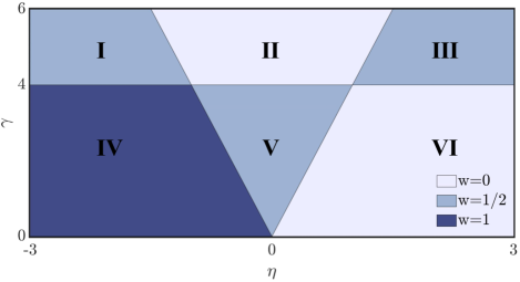
Figure 5: The phase diagram of the non-Hermitian Su-Schrieffer-Heeger model. Here, each phase is labeled by a Roman numeral.

The expression of biorthogonal dynamical phase can be generalized directly from the definition in Hermitian case,

$$\phi_{k}^{\text{dyn}}(t)= -\text{i}\int_{0}^{t}ds\frac{\langle\widetilde{u}_{k-}^{i}(s)|}{\sqrt{\langle\widetilde{u}_{k-}^{i}(s)|u_{k-}^{i}(s)\rangle}}\frac{d}{ds}\frac{|u_{k-}^{i}(s)\rangle}{\sqrt{\langle\widetilde{u}_{k-}^{i}(s)|u_{k-}^{i}(s)\rangle}}$$

$$= -\text{i}\int_{0}^{t}ds[\frac{\langle\widetilde{u}_{k-}^{i}(s)|}{\sqrt{\langle\widetilde{u}_{k-}^{i}(s)|u_{k-}^{i}(s)\rangle}}\frac{\frac{d}{ds}|u_{k-}^{i}(s)\rangle}{\sqrt{\langle\widetilde{u}_{k-}^{i}(s)|u_{k-}^{i}(s)\rangle}}$$

$$+\frac{\langle\widetilde{u}_{k-}^{i}(s)|u_{k-}^{i}(s)\rangle}{\sqrt{\langle\widetilde{u}_{k-}^{i}(s)|u_{k-}^{i}(s)\rangle}}\frac{d}{ds}(\frac{1}{\sqrt{\langle\widetilde{u}_{k-}^{i}(s)|u_{k-}^{i}(s)\rangle}})]$$

$$= -\int_{0}^{t}ds\frac{\langle\widetilde{u}_{k-}^{i}(s)|H_{k}^{f}|u_{k-}^{i}(s)\rangle}{\langle\widetilde{u}_{k-}^{i}(s)|u_{k-}^{i}(s)\rangle}$$

$$+\frac{\text{i}}{2}\text{ln}[\langle\widetilde{u}_{k-}^{i}(t)|u_{k-}^{i}(t)\rangle].$$ (22)

Appendix C More detailed information of biorthogonal DQPTs

As shown in Fig. 5, each phase of non-Hermitian Su-Schrieffer-Heeger model is labeled by a Roman numeral. Various quench processes and the corresponding Fisher zeros and biorthogonal DTOPs are listed in Table 1. The first column specifies the type of quench between different phases. The second column provides concrete parameters $(\eta,\ \gamma)$ of such a quench, where the direction of the arrow “$\rightarrow$” and “$\leftarrow$” denotes the direction of quench. The “Fisher zeros profile” column indicates the possible number of Fisher zeros of a branch $z_{n}(k)$ for a fixed $n$. As mentioned in the main text, a DQPT corresponds to a Fisher zero. Thus the number of Fisher zeros corresponds to the number of DQPTs in this $z_{n}(k)$ branch. The final column indicates the possible value of the change in DTOP that may occur during this quench process.

Table 1: Comparison of various quench processes, exhibiting rich behavior of biorthogonal DQPTs in a single non-Hermitian Hamiltonian.

Quench	Parameters	Fisher zeros profile	DTOP
I $\leftrightarrow$ II	(-2, 5)$\leftrightarrow$(0.2, 5)	$\rightarrow:0,1;\ \leftarrow:2$	$\rightarrow:1;\ \leftarrow:\frac{1}{2}$
I $\leftrightarrow$ III	(-2, 5)$\leftrightarrow$(2, 5)	$\rightarrow:1;\ \leftarrow:1$	$\rightarrow:1;\ \leftarrow:1$
II $\leftrightarrow$ III	(0.2, 5)$\leftrightarrow$(2, 5)	$\rightarrow:2,3;\ \leftarrow:0$	$\rightarrow:\frac{1}{2},1;\ \leftarrow:0$
IV $\leftrightarrow$ V	(-2, 1)$\leftrightarrow$(0.2, 1)	$\rightarrow:1;\ \leftarrow:3,\;4$	$\rightarrow:1;\ \leftarrow:\frac{1}{2},1$
IV $\leftrightarrow$ VI	(-2, 1)$\leftrightarrow$(2, 1)	$\rightarrow:2;\ \leftarrow:2$	$\rightarrow:1;\ \leftarrow:1$
V $\leftrightarrow$ VI	(0, 1)$\leftrightarrow$(2, 1)	$\rightarrow:3,4;\ \leftarrow:1$	$\rightarrow:\frac{1}{2},1;\ \leftarrow:1$
I $\leftrightarrow$ I	(-2, 5)$\leftrightarrow$(-3, 5)	$\leftrightarrow$: 0, 1	$\leftrightarrow$: 1
II $\leftrightarrow$ II	(0.2, 5)$\leftrightarrow$(-0.2, 5)	$\leftrightarrow$: 0, 1	$\leftrightarrow$: $\frac{1}{2}$
III $\leftrightarrow$ III	(2, 5)$\leftrightarrow$(3, 5)	$\leftrightarrow$: 1	$\leftrightarrow$: 1
IV $\leftrightarrow$ IV	(-2, 1)$\leftrightarrow$(-1, 1)	$\leftrightarrow$: 0, 2	$\leftrightarrow$: 1
V $\leftrightarrow$ V	(0.2, 1)$\leftrightarrow$(-0.2, 1)	$\leftrightarrow$: 1, 2	$\leftrightarrow$: $\frac{1}{2}$, 1
VI $\leftrightarrow$ VI	(0.5, 1)$\leftrightarrow$(5, 1)	$\leftrightarrow$: 0, 2	$\leftrightarrow$: 1

This work is supported by the National Natural Science Foundation of China Grants No. 12204075, 11974064, 12075040 and 12147102, the China Postdoctoral Science Foundation Grants No. 2023M730420, the fellowship of Chongqing Postdoctoral Program for Innovative Talents Grant No. CQBX202222, the Natural Science Foundation of Chongqing Grant No. CSTB2023NSCQ-MSX0953, the Chongqing Research Program of Basic Research and Frontier Technology Grants No. cstc2021jcyjmsxmX0081 and cstc2020jcyj-msxmX0890, Chongqing Talents: Exceptional Young Talents Project No. cstc2021ycjh-bgzxm0147, and the Fundamental Research Funds for the Central Universities Grant No. 2020CDJQY-Z003, 2022CDJJCLK001 and 2021CDJQY-007.

References

- (1) I. Rotter, A non-Hermitian Hamilton operator and the physics of open quantum systems, J. Phys. A: Math. Theor. 42, 153001 (2009).
- (2) T. Yoshida, R. Peters, and N. Kawakami, Non-Hermitian perspective of the band structure in heavy-fermion systems, Phys. Rev. B 98, 035141 (2018).
- (3) H. Shen and L. Fu, Quantum Oscillation from In-Gap States and a Non-Hermitian Landau Level Problem, Phys. Rev. Lett. 121, 026403 (2018).
- (4) Y. Nagai, Y. Qi, H. Isobe, V. Kozii, and L. Fu, DMFT Reveals the Non-Hermitian Topology and Fermi Arcs in Heavy-Fermion Systems, Phys. Rev. Lett. 125, 227204 (2020).
- (5) K. G. Makris, R. El-Ganainy, D. N. Christodoulides, and Z. H. Musslimani, Beam Dynamics in PT Symmetric Optical Lattices, Phys. Rev. Lett. 100, 103904 (2008).
- (6) S. Klaiman, U. Günther, and N. Moiseyev, Visualization of Branch Points in PT-Symmetric Waveguides, Phys. Rev. Lett. 101, 080402 (2008).
- (7) S. Malzard, C. Poli, and H. Schomerus, Topologically Protected Defect States in Open Photonic Systems with Non-Hermitian Charge-Conjugation and Parity-Time Symmetry, Phys. Rev. Lett. 115, 200402 (2015).
- (8) C. M. Bender and S. Boettcher, Real Spectra in Non-Hermitian Hamiltonians Having PT Symmetry, Phys. Rev. Lett. 80, 5243 (1998).
- (9) T. Helbig, T. Hofmann, S. Imhof, M. Abdelghany, T. Kiessling, L. W. Molenkamp, C. H. Lee, A. Szameit, M. Greiter, and R. Thomale, Generalized bulk-boundary correspondence in non-Hermitian topolectrical circuits, Nat. Phys. 16, 747 (2020).
- (10) S. Liu, R. Shao, S. Ma, L. Zhang, O. You, H. Wu, Y. J. Xiang, T. J. Cui, and S. Zhang, Non-Hermitian Skin Effect in a Non-Hermitian Electrical Circuit, Research 2021, 5608038 (2021).
- (11) S. Weidemann, M. Kremer, T. Helbig, T. Hofmann, A. Stegmaier, M. Greiter, R. Thomale, and A. Szameit, Topological funneling of light, Science 368, 311 (2020).
- (12) M. Brandenbourger, X. Locsin, E. Lerner, and C. Coulais, Non-reciprocal robotic metamaterials, Nat. Commun. 10, 4608 (2019).
- (13) A. Ghatak, M. Brandenbourger, J. V. Wezel, and C. Coulais, Observation of non-Hermitian topology and its bulk-edge correspondence in an active mechanical metamaterial, Proc. Natl. Acad. Sci. USA 117, 29561 (2020).
- (14) X. Zhang, Y. Tian, J.-H. Jiang, M.-H. Lu, and Y.-F. Chen, Observation of higher-order non-Hermitian skin effect, Nat. Commun. 12, 5377 (2021).
- (15) L. Zhang, Y. Yang, Y. Ge, Y.-J. Guan, Q. Chen, Q. Yan, F. Chen, R. Xi, Y. Li, D. Jia, S.- Q. Yuan, H.-X. Sun, H. Chen, and B. Zhang, Acoustic non-Hermitian skin effect from twisted winding topology, Nat. Commun. 12, 6297 (2021).
- (16) L. Xiao, T. Deng, K. Wang, G. Zhu, Z. Wang, W. Yi, and P. Xue, Non-Hermitian bulk-boundary correspondence in quantum dynamics, Nat. Phys. 16, 761 (2020).
- (17) H. Wang, X. Zhang, J. Hua, D. Lei, M. Lu, and Y. Chen, Topological physics of non-Hermitian optics and photonics: a review, J. Opt. 23, 123001 (2021).
- (18) S. Yao and Z. Wang, Edge States and Topological Invariants of Non-Hermitian Systems, Phys. Rev. Lett. 121, 086803 (2018).
- (19) K. Kawabata, K. Shiozaki, M. Ueda, and M. Sato, Symmetry and Topology in Non-Hermitian Physics, Phys. Rev. X 9, 041015 (2019).
- (20) K. Yokomizo and S. Murakami, Non-Bloch Band Theory of Non-Hermitian Systems, Phys. Rev. Lett. 123, 066404 (2019).
- (21) H. Shen, B. Zhen, and L. Fu, Topological Band Theory for Non-Hermitian Hamiltonians, Phys. Rev. Lett. 120, 146402 (2018).
- (22) H. Hodaei, A. U. Hassan, S. Wittek, H. Garcia-Gracia, R. El-Ganainy, D. N. Christodoulides, and M. Khajavikhan, Enhanced sensitivity at higher-order exceptional points, Nature (London) 548, 187 (2017).
- (23) E. J. Bergholtz, J. C. Budich, and F. K. Kunst, Exceptional topology of non-Hermitian systems, Rev. Mod. Phys. 93, 015005 (2021).
- (24) K. Zhang, Z. Yang, and C. Fang, Correspondence between Winding Numbers and Skin Modes in Non-Hermitian Systems, Phys. Rev. Lett. 125, 126402 (2020).
- (25) X. Zhang, T. Zhang, M.-H. Lu, and Y.-F. Chen, A review on non-Hermitian skin effect, Adv. Phys.: X 7, 2109431 (2022).
- (26) H. Zhou, C. Peng, Y. Yoon, C. W. Hsu, K. A. Nelson, L. Fu, J. D. Joannopoulos, M. Soljacic, and B. Zhen, Observation of bulk Fermi arc and polarization half charge from paired exceptional points, Science, 359, 1009 (2018).
- (27) Y. Ashida, Z. Gong, and M. Ueda, Non-Hermitian physics, Adv. Phys. 69, 249 (2020).
- (28) D. C. Brody, Biorthogonal quantum mechanics, J. Phys. A: Math. Theor. 47, 035305 (2014).
- (29) F. K. Kunst, E. Edvardsson, J. C. Budich, and E. J. Bergholtz, Biorthogonal Bulk-Boundary Correspondence in Non-Hermitian Systems, Phys. Rev. Lett. 121, 026808 (2018).
- (30) E. Edvardsson, F. K. Kunst, and E. J. Bergholtz, Non-Hermitian extensions of higher-order topological phases and their biorthogonal bulk-boundary correspondence, Phys. Rev. B 99, 081302(R) (2019).
- (31) E. Edvardsson, F. K. Kunst, T. Yoshida, and E. J. Bergholtz, Phase transitions and generalized biorthogonal polarization in non-Hermitian systems, Phys. Rev. Res. 2, 043046 (2020).
- (32) Z. Xu and S. Chen, Dynamical evolution in a one-dimensional incommensurate lattice with symmetry, Phys. Rev. A 103, 043325 (2021).
- (33) L. Pan, X. Chen, Y. Chen and H. Zhai, Non-Hermitian linear response theory, Nat. Phys. 16, 767 (2020).
- (34) Z. Lin, L. Zhang, X. Long, Y.-a. Fan, Y. Li, K. Tang, J. Li, X. Nie, T. Xin, X.-J. Liu, and D. Lu, Experimental quantum simulation of non-Hermitian dynamical topological states using stochastic Schrödinger equation, npj Quantum Inf. 8, 77 (2022).
- (35) H. Liu, X. Yang, K. Tang, L. Che, X. Nie, T. Xin, J. Li, and D. Lu, Practical quantum simulation of small-scale non-Hermitian dynamics, Phys. Rev. A 107, 062608 (2023).
- (36) K. T. Geier and P. Hauke, From Non-Hermitian Linear Response to Dynamical Correlations and Fluctuation-Dissipation Relations in Quantum Many-Body Systems, PRX Quantum 3, 030308 (2022).
- (37) K. Kawabata, T. Numasawa, and S. Ryu, Entanglement Phase Transition Induced by the Non-Hermitian Skin Effect, Phys. Rev. X 13, 021007 (2023).
- (38) T. Yoshimura, K. Bidzhiev, and H. Saleur, Non-Hermitian quantum impurity systems in and out of equilibrium: Noninteracting case, Phys. Rev. B 102, 125124 (2020).
- (39) A. McDonald, R. Hanai, and A. A. Clerk, Nonequilibrium stationary states of quantum non-Hermitian lattice models, Phys. Rev. B 105, 064302 (2022).
- (40) L.-J. Zhai, G.-Y. Huang, and S. Yin, Nonequilibrium dynamics of the localization-delocalization transition in the non-Hermitian Aubry-André model, Phys. Rev. B 106, 014204 (2022).
- (41) K. D. Agarwal, T. K. Konar, L. G. C. Lakkaraju, and A. Sen, Detecting Exceptional Point through Dynamics in Non-Hermitian Systems,arXiv:2212.12403.
- (42) K. D. Agarwal, T. K. Konar, L. G. C. Lakkaraju, and A. Sen, Recognizing critical lines via entanglement in non-Hermitian systems, arXiv:2305.08374.
- (43) A. S. M.-Roubeas, F. Roccati, J. Cornelius, Z. Xu, A. Chenu, and A. D. Campo, Non-Hermitian Hamiltonian deformations in quantum mechanics, J. High Energ. Phys. 2023, 60 (2023).
- (44) M. Heyl, A. Polkovnikov, and S. Kehrein, Dynamical Quantum Phase Transitions in the Transverse-Field Ising Model, Phys. Rev. Lett. 110, 135704 (2013).
- (45) J. C. Budich and M. Heyl, Dynamical topological order parameters far from equilibrium, Phys. Rev. B 93, 085416 (2016).
- (46) J.-J. Dong and Y.-F. Yang, Functional field integral approach to quantum work, Phys. Rev. B 100, 035124 (2019).
- (47) X. Nie, B.-B. Wei, X. Chen, Z. Zhang, X. Zhao, C. Qiu, Y. Tian, Y. Ji, T. Xin, D. Lu, and J. Li, Experimental Observation of Equilibrium and Dynamical Quantum Phase Transitions via Out-of-Time-Ordered Correlators, Phys. Rev. Lett. 124, 250601 (2020).
- (48) Y. Zeng, B. Zhou, and S. Chen, Dynamical singularity of the rate function for quench dynamics in finite-size quantum systems, Phys. Rev. B 107, 134302 (2023).
- (49) M. Heyl and J. C. Budich, Dynamical topological quantum phase transitions for mixed states, Phys. Rev. B 96, 180304(R) (2017).
- (50) U. Bhattacharya, S. Bandyopadhyay, and A. Dutta, Mixed state dynamical quantum phase transitions, Phys. Rev. B 96, 180303(R) (2017).
- (51) N. O. Abeling and S. Kehrein, Quantum quench dynamics in the transverse field Ising model at nonzero temperatures, Phys. Rev. B 93, 104302 (2016).
- (52) N. Sedlmayr, M. Fleischhauer, and J. Sirker, Fate of dynamical phase transitions at finite temperatures and in open systems, Phys. Rev. B 97, 045147 (2018).
- (53) J. Lang, B. Frank, and J. C. Halimeh, Dynamical Quantum Phase Transitions: A Geometric Picture, Phys. Rev. Lett. 121, 130603 (2018).
- (54) J. Lang, B. Frank, and J. C. Halimeh, Concurrence of dynamical phase transitions at finite temperature in the fully connected transverse-field Ising model, Phys. Rev. B 97, 174401 (2018).
- (55) K. Yang, L. Zhou, W. Ma, X. Kong, P. Wang, X. Qin, X. Rong, Y. Wang, F. Shi, J. Gong, and J. Du, Floquet dynamical quantum phase transitions, Phys. Rev. B 100, 085308 (2019).
- (56) J. Naji, M. Jafari, R. Jafari, and A. Akbari, Dissipative Floquet Dynamical Quantum Phase Transition, Phys. Rev. A 105, 022220 (2022).
- (57) R. Jafari and A. Akbari, Floquet dynamical phase transition and entanglement spectrum, Phys. Rev. A 103, 012204 (2021).
- (58) R. Jafari, A. Akbari, U. Mishra, and H. Johannesson, Floquet dynamical quantum phase transitions under synchronized periodic driving, Phys. Rev. B 105, 094311 (2022).
- (59) S. Sharma, U. Divakaran, A. Polkovnikov, and A. Dutta, Slow quenches in a quantum Ising chain: Dynamical phase transitions and topology, Phys. Rev. B 93, 144306 (2016).
- (60) P. Jurcevic, H. Shen, P. Hauke, C. Maier, T. Brydges, C. Hempel, B. P. Lanyon, M. Heyl, R. Blatt, and C. F. Roos, Direct Observation of Dynamical Quantum Phase Transitions in an Interacting Many-Body System, Phys. Rev. Lett. 119, 080501 (2017).
- (61) J. Zhang, G. Pagano, P. W. Hess, A. Kyprianidis, P. Becker, H. Kaplan, A. V. Gorshkov, Z.-X. Gong, and C. Monroe, Observation of a many-body dynamical phase transition with a 53-qubit quantum simulator, Nature (London) 551, 601 (2017).
- (62) H. Bernien, S. Schwartz, A. Keesling, H. Levine, A. Omran, H. Pichler, S. Choi, A. S. Zibrov, M. Endres, M. Greiner, V. Vuletic, and M. D. Lukin, Probing many-body dynamics on a 51-atom quantum simulator, Nature (London) 551, 579 (2017).
- (63) N. Fläschner, D. Vogel, M. Tarnowski, B. S. Rem, D.-S. Lühmann, M. Heyl, J. C. Budich, L. Mathey, K. Sengstock, and C. Weitenberg, Observation of dynamical vortices after quenches in a system with topology, Nat. Phys. 14, 265 (2018).
- (64) X.-Y. Guo, C. Yang, Y. Zeng, Y. Peng, H.-K. Li, H. Deng, Y.-R. Jin, S. Chen, D. Zheng, and H. Fan, Observation of a Dynamical Quantum Phase Transition by a Superconducting Qubit Simulation, Phys. Rev. Appl. 11, 044080 (2019).
- (65) T. Tian, Y. Ke, L. Zhang, S. Lin, Z. Shi, P. Huang, C. Lee, and J. Du, Observation of dynamical phase transitions in a topological nanomechanical system, Phys. Rev. B 100, 024310 (2019).
- (66) K. Wang, X. Qiu, L. Xiao, X. Zhan, Z. Bian, W. Yi, and P. Xue, Simulating Dynamic Quantum Phase Transitions in Photonic Quantum Walks, Phys. Rev. Lett. 122, 020501 (2019).
- (67) X.-Y. Xu, Q.-Q. Wang, M. Heyl, J. C. Budich, W.-W. Pan, Z. Chen, M. Jan, K. Sun, J.-S. Xu, Y.-J. Han, C.-F. Li, and G.-C. Guo, Measuring a dynamical topological order parameter in quantum walks, Light Sci. Appl. 9, 7 (2020).
- (68) D. Mondal and T. Nag, Anomaly in dynamical quantum phase transition in non-Hermitian system with extended gapless phases, Phys. Rev. B 106, 054308 (2022).
- (69) L. Zhou, Q.-H. Wang, H. Wang, and J. Gong, Dynamical quantum phase transitions in non-Hermitian lattices, Phys. Rev. A 98, 022129 (2018).
- (70) L. Zhou and Q. Du, Non-Hermitian topological phases and dynamical quantum phase transitions: a generic connection, New J. Phys. 23, 063041 (2021).
- (71) D. Mondal and T. Nag, Finite temperature dynamical quantum phase transition in a non-Hermitian system, arXiv:2212.05839.
- (72) G. Sun, J.-C. Tang, and S.-P. Kou, Biorthogonal quantum criticality in non-Hermitian many-body systems, Front. Phys. 17, 33502 (2022).
- (73) J.-C. Tang, S.-P. Kou, and G. Sun, Dynamical scaling of Loschmidt echo in non-Hermitian systems, Europhys. Lett. 137, 40001 (2022).
- (74) S. Vajna and B. Dóra, Topological classification of dynamical phase transitions, Phys. Rev. B 91, 155127 (2015).
- (75) C. Yin, H. Jiang, L. Li, R. Lü, and S. Chen, Geometrical meaning of winding number and its characterization of topological phases in one-dimensional chiral non-Hermitian systems, Phys. Rev. A 97, 052115 (2018).
- (76) C. Ding, Dynamical quantum phase transition from a critical quantum quench, Phys. Rev. B 102, 060409(R) (2020).
- (77) M. E. Fisher, The theory of equilibrium critical phenomena, Rep. Prog. Phys. 30, 615 (1967).
- (78) C. N. Yang and T. D. Lee, Statistical Theory of Equations of State and Phase Transitions. I. Theory of Condensation, Phys. Rev. 87, 404 (1952).
- (79) T. D. Lee and C. N. Yang, Statistical Theory of Equations of State and Phase Transitions. II. Lattice Gas and Ising Model, Phys. Rev. 87, 410 (1952).
- (80) J. Zakrzewski, Dynamical quantum phase transitions from quantum optics perspective, arXiv:2204.09454.