MULTI-MODAL MULTI-CLASS PARKINSON DISEASE CLASSIFICATION USING CNN and DECISION LEVEL FUSION

Abstract

Parkinson’s disease (PD) is the second most common neurodegenerative disorder, as reported by the World Health Organization (WHO). In this paper, we propose a direct three-Class PD classification using two different modalities, namely, MRI and DTI. The three classes used for classification are PD, Scans Without Evidence of Dopamine Deficit (SWEDD) and Healthy Control (HC). We use white matter (WM) and gray matter (GM) from the MRI and fractional anisotropy (FA) and mean diffusivity (MD) from the DTI to achieve our goal. We train four separate CNNs on the above four types of data. At the decision level, the outputs of the four CNN models are fused with an optimal weighted average fusion technique. We achieve an accuracy of 95.53% for the direct three-class classification of PD, HC and SWEDD on the publicly available PPMI database. Extensive comparisons including a series of ablation studies clearly demonstrate the effectiveness of our proposed solution.

1 Introduction

Parkinson’s disease is the second most common neurological disorder that affects movement and can cause tremors, stiffness, and difficulty with coordination  [1]. Early diagnosis of PD is important for effective treatment, as there is currently no cure for the disease. However, diagnosis can be challenging due to the variability of symptoms and lack of definitive biomarkers. According to the World Health Organization (WHO), PD affects approximately 1% of people aged 60 years and older worldwide. However there are approximately 10% of clinically diagnosed patients with early stage PD who exhibit normal dopaminergic functional scans. This class, which signifies a medical condition distinct from PD, is known as Scans Without Evidence of Dopamine Deficit (SWEDD) [2, 3]. As a result of the evolution of this new class, difficulty of diagnosing PD has increased manifold, leading to a three-class classification problem of PD vs. SWEDD vs. HC with class overlaps [3].

MRI, SPECT and PET are commonly used imaging techniques for PD diagnosis. However, PET and SPECT are not preferred by doctors due to invasiveness and cost  [4]. DTI is a newer technique that measures water molecule movement to analyze white matter microstructure which gets affected in PD. In the literature, quite a few works were reported on PD classification based on machine learning (ML) and deep learning (DL) models applied to neuroimaging data. Salat et al. [5] found correlations between gray or white matter changes and age using Voxel-based Morphometry (VBM). Adeli et al. [1] used a recursive feature elimination approach for two-class classification with 81.9 % accuracy. Cigdem et al. [6] proposed a total intracranial volume method with 93.7% accuracy. Singh et al. [2] presented a ML framework for three two-class classifications. Chakraborty et al. [7] presented an DL model with 95.29% accuracy. A DL-based ensemble learning technique was reported by [8] with 97.8% accuracy.

Recent research indicates that combining features from more than one imaging modality can improve the classification accuracy. For example, Li et al. [9] showed that combining DTI and MRI features improves the classification accuracy in Alzheimer’s disease. The authors of [10] used MRI and DTI, but only considered MD data from DTI for PD classification. They used a stacked sparse auto-encoder to achieve better classification accuracy. In light of the above findings, we anticipate that MRI and DTI can be effectively combined to better analyze PD. To increase decision accuracy, we mention here a few decision level fusion techniques. Majority voting technique is the most common techniques used in late fusion  [11]. This strategy, however, may not be appropriate for multi-class classification applications. Single classifiers work well on most subjects, but error rates are enhanced for some difficult-to-classify subjects due to overlap across many categories. Instead of using a majority voting strategy, a modified scheme called modulated rank averaging is employed in [12]. We feel the accuracy may be enhanced even further by fine-tuning the weights computed in the modulated rank averaging approach.

As a summary, we can say that there is a clear dearth of direct three-class PD classification strategies and that too with multi-modal data. In this paper, we present a direct three-class PD classification using CNNs and decision level fusion. We investigate full potential of multimodal data i.e., FA & MD from DTI and WM & GM from MRI. We use four CNNs to analyze these four types of data. Outputs from all these four models are finally fused using an Optimal Weighted Average Fusion (OWAF) technique at the decision level. Since neuroimaging datasets are small, data augmentation is adopted to ensure proper training with the CNNS [12]. We now summarize our contributions as below:

1. We address a direct three-class classification task (PD, HC and SWEDD) for Parkinson’s disease, which is certainly more challenging than the current trend of a single binary classification (for 2-class problem) or multiple binary classifications (for 3-class problem).

2. We make effective use of the underlying potential of multi-modal neuroimaging, namely T1-weighted MRI and DTI. In particular, we train four different CNNs on WM, GM data from MRI and FA, MD data from DTI. Such in-depth analysis of multi-modal neuroimaging data is largely missing in the analysis of PD.

3. Finally, at the decision level, the outputs of each CNN model are fused using an Optimal Weighted Average Fusion (OWAF) strategy to achieve state-of-the-art classification accuracy.

2 Proposed method

Our solution pipeline for an end-to-end direct three-class classification of PD from DTI and MRI consists of four CNN networks. Each CNN network yields a $3\times 1$ probability vector, which represents the probability that the data falls into one of three classes, i.e., PD, HC or SWEDD. The probability vectors are then combined using the OWAF technique. In section 2.1, we discuss how WM and GM are obtained from MRI data and MD and FA are used from DTI data. Section 2.2 describes ADASYN, an oversampling strategy. Section 2.3 presents the proposed CNN architecture. In section 2.4, we discuss the decision level fusion. Figure 1 illustrates the overall pipeline of our solution.

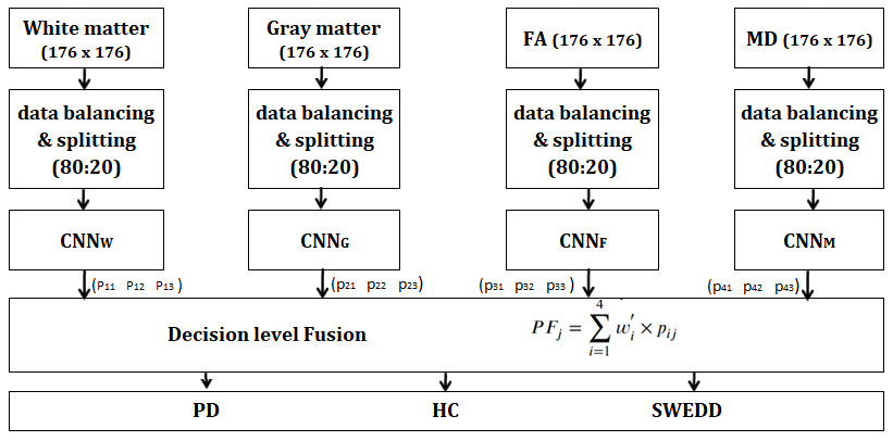
Figure 1: Direct three-class Parkinson’s disease classification framework

2.1 Data Pre-processing

In this work, voxel-based morphometry (VBM) is used to prepare MRI data. The data is preprocessed using SPM-12 tools and images are normalized using the diffeomorphic anatomical registration with exponentiated lie algebra (DARTEL) method  [13]. This SPM-12 tool segments the whole MRI data into GM, WM and cerebrospinal fluid, as well as the anatomical normalization of all images to the same stereotactic space employing linear affine translation, non-linear warping, smoothing and statistical analysis. After registration, GM and WM volumetric images were obtained and the unmodulated image is defined as the density map of grey matter (GMD) and white matter (WMD). The PPMI database contains all information regarding DTI indices, including FA and MD. Brain scans from PD groups as well as HC have distinct voxel MD values. MD and FA can be expressed mathematically expressed as  [14]:

$$MD=\frac{\lambda_{1}+\lambda_{2}+\lambda_{3}}{3}=\frac{D_{xx}+D_{yy}+D_{zz}}{3}$$ (1)

$$FA=\sqrt{\frac{1}{2}}\sqrt{\frac{{(\lambda_{1}-\lambda_{2})}^{2}+{(\lambda_{2}-\lambda_{3})}^{2}+{(\lambda_{3}-\lambda_{1})}^{2}}{{\lambda_{1}}^{2}+{\lambda_{2}}^{2}+{\lambda_{3}}^{2}}}$$ (2)

In equations 1 the diagonal terms of the diffusion tensor are $D_{xx},D_{yy}andD_{zz}$ and the sum of these diagonal terms constitutes its trace. After prepossessing, four types of data are made available, namely, grey matter (GM), white matter (WM), fractional anisotropy (FA) and mean diffusivity (MD).

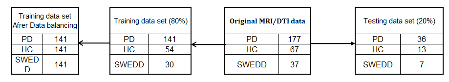
Figure 2: Dataset division strategy

2.2 Data balancing with ADASYN

We find each of GM, WM, FA, MD to be highly imbalanced across the three classes. Further, the number of training samples required to feed a DL model is insufficient. So, ADASYN, an oversampling method is used to increase the number of samples for each minority class  [15]. The primary idea behind the use of an ADASYN technique is to compute the weighted distribution of minority samples based on a wide range of out-of-elegance neighbors. A difficult-to-train minority instance surrounded by more out-of-class examples is given a better chance of being augmented through producing synthetic samples. Using a set of pseudo-probabilistic rules, a predetermined number of instances are generated for every minority class depending on the weighted distribution of its neighbors. Following the implementation of this up-sampling approach, the total number of samples in each of the classes is 141 volumetric images. The details of data set division strategies are shown in Figure 2.

Let a dataset consists of $m$ samples of the form $({x_{i},y_{i}})$; where $i\in[1,m]$, $x_{i}$ being the $i^{th}$ sample of the n-dimensional feature space X and $y_{i}$ being the label (class) of the sample ${x_{i}}$. Let $m_{min}$ and $m_{maj}$ be number of the minority and majority class samples respectively. Then the ratio of minority to majority sample will be expressed as: d = $m_{min}$ /$m_{maj}$. Let, $\beta$ be the balance level of the synthetic samples. So, $\beta=1$ represents that both the classes are balanced using ADASYN. Number of synthetic minority data to be created is given by: 3.

$$G=(m_{maj}-m_{min})\times\beta$$ (3)

For $\beta\neq 1$, synthetic samples will be created for each set of minority data based on the Euclidean distance of their k-nearest neighbors. The dominates of the majority class in each neighborhood is expressed as: $r_{i}=\frac{\Delta_{i}}{k}$. where $\Delta_{i}$ is the number of examples in the k-nearest neighbors of $x_{i}$ that belong to the majority class. Higher value of ${r_{i}}$ in a neighborhood indicates more examples of the majority class which makes them harder to learn. We next determine how many synthetic samples per neighborhood need to be generated as: $G_{i}=G\times\hat{r_{i}}$. Here $\hat{r_{i}}$ represent normalized version of ${r_{i}}$. This captures the adaptive nature of the ADASYN algorithm, which means more data is created for harder to learn neighbourhoods. We generate $G_{i}$ number of synthetic data ${s_{i,j},j=1,2,\cdots,G_{i}}$ for each neighbourhood $i$ as shown in equation 4 below:

$${s_{i,j}}=x_{i}+(x_{zi}-x_{i})\times\lambda$$ (4)

Where $x_{i}$ and $x_{zi}$ are two minority occurrences in the same neighborhood and $\lambda$ is a random integer between 0 and 1. In our work, these synthetic images are generated with the help of the Scikit-Learn library such that all the classes are balanced in nature.

2.3 Proposed CNN Architecture

We use four CNN models, each with ten convolutional layers and four dense (FC) layers, for the direct three-class classification task of PD. The proposed network’s architecture is depicted in Figure 3. We chose fewer parameters in the proposed architecture than in the original VGG16  [16] by decreasing network depth. Our proposed network is similar to that proposed in  [17]. The number of layers are limited to maintain a trade-off between accuracy and computational cost. To generate feature representations of brain MR scans, convolution layers are used. The final FC layer and a soft max operation are used for the classification task. The volumetric input data is processed slice-wise, with each slice having a size of $176\times 176$ pixels. We have used max-pooling in the pooling layers to reduce the image size. The flattened layers convert the reduced feature maps to a one-dimensional feature map. The fully connected layers classify this feature map into three classes: HC, PD and SWEDD. The cross-entropy loss function (CELF) is the most common loss function used for classification problems since it has better convergence speeds for training deep CNNs than MSE and hinge loss. As a result, we consider CELF for this work, which is mathematically expressed as:

$$L_{CELF}=-\sum\limits_{i=1}^{N}\sum\limits_{j=1}^{K}p(y_{j}|\mathbf{x})\log\widehat{p}\left({y_{j}|\mathbf{x}}\right)$$ (5)

where $p(y_{j}|\mathbf{x})$ is the original class label distribution and $\widehat{p}(y_{j}|\mathbf{x})$ is the predicted label distribution from the CNN network. Here $N$ and $K$ represent the number of models and number of classes respectively. For our problem, $N=4$ and $K=3$.

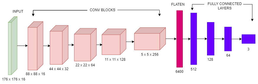
Figure 3: Architecture of the proposed CNN

2.4 Decision Level Fusion of CNN Networks

We use four CNN models, one each for GM, WM, FA and MD. We fuse these predicted probabilities with the help of suitable weights. The weights are generated in two stages. In the first stage, the weights are generated using the modulated rank averaging (MRA) method  [12]. The weights in the MRA method are given by:

$$w_{i}=\frac{f_{i}}{\sum_{i=1}^{N-1}f_{i}+R_{max}}$$ (6)

In equation 6, $f_{i}$ and $R_{max}$ indicate the normalizing factor and the rank of the model having highest accuracy respectively. The normalizing factor is calculated based on the rank of the current model and the difference between the accuracy of the current and next model. In the second stage, these weights are optimised using the grid search method  [18]. Let the final optimized weights be denoted by $w_{i}^{{}^{\prime}}$. Note that this weight vector is fixed for all 3 classes. We combine this optimal weight vector with the respective probability vectors to obtain the overall probability of occurrence of respective classes. Let us denote by $PF_{j};j=1,2,3$, the overall probability of occurrence of the $j^{th}$ class as a result of fusion.

$$PF_{j}=\sum_{i=1}^{4}w_{i}^{{}^{\prime}}\times p_{ij}$$ (7)

The final class will be the one for which $PF_{j}$ is maximum.

Table 1: Demographics of the subjects

	Healthy Control	Parkinson’s Disease	SWEDD
Number of subjects	67	177	37
Sex (Female/Male)	24/43	65/122	14/23
Age*	60.12 ±10.71	61.24 ±9.47	59.97 ±10.71
*mean ± standard deviation

3 Experimental Results

In this section we present the experimental results for three class PD classification. The section is divided into three subsections. In the first subsection, we provide an overview of the PPMI database. We then discuss data preparation, computing configuration, parameter settings of ADASYN and CNN and evaluation metrics. The second subsection shows a series of ablation studies to demonstrate separate impacts of both MRI and DTI data and the proposed fusion strategy. Finally, we include comparisons with several state-of-the-art methods to demonstrate the effectiveness of the proposed solution.

3.1 Data preparation and implementation details

In our study, we included 281 subjects with baseline visits having both DTI and MRI data from PPMI. This includes 67 HC, 177 PD and 37 SWEDD subjects. Table 1 shows the demographics of the individuals used in this investigation. For all experiments, we use a system with 16.0 GB DDR4 RAM, an Intel® Core™ i7-10750H CPU @ 2.60GHz and GPU of NVIDIA GeForse RTX 3060 @ 6GB. Here, 80% of the data were randomly selected from the PD, SWEDD and HC groups to produce the training set from 225 volumetric image scans. The remaining 56 volumetric image scans, representing approximately 20% of each class, were utilized to create the test set. For ADASYN, we experiment with different neighbor counts (k) on the training set while keeping other settings unaltered. We find that k = 30 produced the best results. Figure 2 shows the details of data set division strategies. As a result of this, the total number of volumetric images becomes 423, where each of the three classes have 141 volumetric images. For the four CNN models, one each on GM, WM, FA and MD data, we train the network for 100 epochs. ADAM optimizer and ReLU activation functions are employed. The learning rate is initialized at $1\times 10^{-4}$ with a batch size of 32. We use the same training parameters for each model (WM, GM, FA and MD) such that there are no conflicts when we combine the outputs of the models and make a fusion at the decision level. We evaluate the classification performance using four different metrics. These are accuracy, precision, recall and F1 score. All the measures are calculated using the Scikit Learn packages  [19].

Table 2: Impact of DTI and MRI data on direct 3-class classification

Data	Accuracy in (%)	Precision in (%)	Recall in (%)	F1 Score in (%)
MRI (WM)	88.6	86.57	82.50	88.94
MRI (GM)	84.2	81.76	82.50	84.80
DTI (MD)	88.2	88.85	89.50	88.11
DTI(FA)	80.94	80.35	81.00	81.59
WM and GM (MRI)	90.02	90.17	90.02	90.09
FA and MD (DTI)	91.14	91.23	91.14	91.18
WM, GM, FA, MD (MRI + DTI) using OWAF	95.53	93.64	91.99	92.74

Table 3: Impact of fusion strategies on direct 3-class classification

Fusion Technique	Accuracy in (%)	Precision in (%)	Recall in (%)	F1 Measure in (%)
Majority Voting	92.19	92.5	94.87	92.34
Model Average Fusion	88.6	82.5	86.57	85.44
Modulated Rank Average	94.6	91.5	93.92	93.02
OWAF (proposed)	95.53	93.64	91.99	92.74

3.2 Ablation Studies

We include two ablation studies. The first study demonstrates the utility of using both MRI and DTI data. The second study conveys the benefit of OWAF, the proposed fusion strategy. The four CNNs are trained and evaluated on both single and multi-modal data from MRI and DTI. Our goal is to investigate the effects of using single and multi-modal data on direct three-class. The results of direct three-class classification are presented in Table 2. This tables clearly illustrate that use of both DTI and MRI yields superior results as compared to using MRI and DTI in isolation. Note that the magnitude of improvement from the use of multi-modal data is clearly more significant for the more challenging three-class classification problem. The four CNNs are combined using four different fusion strategies at the decision level, namely; majority voting, model average fusion, modulated rank averaging  [12] and the proposed optimal weighted average fusion (OWAF) based on the grid search approach. When voting techniques are applied, the universal decision rule is established simply by fusing the decisions made by separate models. In the model average fusion method, the output probabilities of each model are simply multiplied by the weight provided to that model based on its accuracy. In the modulated rank averaging method (MRA), the output probabilities of each model are updated using a weight generated based on their rank and the difference in probabilities between the models. This method gives better results than the model average fusion method and the majority voting method. In this work, we take the weights generated using MRA as the initial weights. These base weights are further optimised using the grid search method. In grid search, we fine tune the weights ($w_{i}$) in the range of $w_{i}\pm 0.05$ with a step size of 0.01. The final weights are used in our OWAF technique. Table 3 illustrates the effects of various fusion strategies. For fare comparison, we use both MRI and DTI data in all cases. The experimental results in the table 3 clearly reveal that the proposed OWAF outperforms other fusion strategies.

Table 4: Comparisons of the proposed method with State-of-the-art Approaches

Approach	ML/DL	MODALITY	PD vs HC			PD vs. SWEDD	HC vs. SWEDD	PD vs. HC vs SWEDD
			Ac	Pr	Re	Ac	Ac	Ac
Adeli 2016 [1]	ML	MRI	81.9	-	-	-	-	-
Cigdem 2018 [6]	ML	MRI	93.7	-	95	-	-	-
Prashanth 2018 [20]	ML	SPECT	95	-	96.7	-	-	-
Singh 2018 [2]	ML	MRI	95.37	-	-	96.04	93.03	-
Gabriel 2021 [21]	ML	MRI	99.01(M) 87.10(F) 93.05 (A)	100(M) 97.2(F) -	99.3(M) 100(F) -	-	-	-
Li 2019 [10]	DL (AE)	MRI + DTI	85.24	95.8	68.1	-	89.67	-
Tremblay 2020 [22]	DL	MRI	88.3	88.2	88.4	-	-	-
Chakraborty 2020 [7]	DL	MRI	95.3	92.7	91.4	-	-	-
Sivaranjini 2020 [23]	DL	MRI	88.9	-	89.3	-	-	-
Rajanbabu 2022 [8]	DL (EL)	MRI	97.5	97.9	97.1	-	-	-
Proposed method	DL	MRI + DTI	97.8	97.2	97.6	94.5	95.7	95.53 Pr: 93.64 Re: 91.99

• Ac, Pr, Re, M, F, A, AE, EL, - Indicates Accuracy, Precision, Recall, Male, Female, Average, Auto Encoder, Ensemble Learning & data not available respectively. All the values are in %.

3.3 Comparisons with State-of-the-art Approaches

We compare our method with ten state-of-the-art approaches. There are no results available for a direct 3-class PD classification. So, we compare our results with those papers that have addressed the PD classification on the PPMI database using single or multiple modalities and with three or fewer two-class classifications. The results of comparisons are shown in Table 4. Out of the ten methods we have considered, five are based on machine learning (ML) and the rest five are based on deep learning (DL). Further, in four out of five DL based approaches, only a single modality, namely, MRI is used for classification. Also note that eight of these ten techniques have only addressed a single two-class classification problem between PD and HC and did not consider the challenging SWEDD class at all. The remaining two approaches did consider SWEDD as a third class but have divided the three-class classification problem into multiple binary classes [2, 10]. However, Li at al. [10] did not report the classification results for PD vs. SWEDD in their paper. In order to have fair comparisons, we have also included three binary classifications as obtained from our method in this table. Our direct three-class classification accuracy turns out to be superior than two-class classification accuracy of at least eight out of 10 methods. It is also higher than two out of three binary classification accuracy of [2]. Note that in [2], the authors used a somewhat different experimental protocol by considering two publicly available databases of ADNI and PPMI. In our work, we explicitly consider data with both MRI and DTI for the same individual as available solely in the PPMI database. Though the authors in [21] reported superior classification accuracy for male, the accuracy is much less for female and also for the average case (both male and female taken into account). Only, [8] has reported a higher classification accuracy than ours. But, they have considered only a single binary class classification of PD vs HC and ignored the more challenging SWEDD class. If we consider the binary classification results of our method, then we straightway outperform nine of the ten state-of-the-art competitors and even beat the remaining method [2] in two out of three classifications.

4 Conclusion

In this paper, we presented an automated solution for the direct three-class classification of PD using both MRI and DTI data. Four different CNNs were used for separate classifications with WM and GM data from MRI and MD and FA data from DTI. An optimal weighted average decision fusion method was applied next to integrate the individual classification outcomes. An overall three-class classification accuracy of 95.53% is achieved. Extensive testing, including a number of ablation studies on the publicly available PPMI database clearly establishes the efficacy of our proposed formulation.

In future, we plan to deploy our model in clinical practice with data from other neuro-imaging modalities. We also plan to to extend our model for classifying other Parkinsonian syndromes.

References

- [1] E. Adeli, F. Shi, L. An, C. Y. Wee, G. Wu, T. Wang, D. Shen, Joint feature-sample selection and robust diagnosis of parkinson’s disease from mri data, NeuroImage 141 (2016) 206–219.
- [2] G. Singh, L. Samavedham, E. C.-H. Lim, Determination of imaging biomarkers to decipher disease trajectories and differential diagnosis of neurodegenerative diseases (disease trend), Journal of Neuroscience Methods 305 (2018) 105–116.
- [3] M. Kim, H. Park, Using tractography to distinguish swedd from parkinson’s disease patients based on connectivity, Parkinson’s Disease 2016, article id: 8704910 (2016).
- [4] D. Long, J. Wang, M. Xuan, Q. Gu, X. Xu, D. Kong, M. Zhang, Automatic classification of early parkinson’s disease with multi-modal mr imaging, PLOS ONE 7 (2012) e47714.
- [5] D. H. Salat, S. Y. Lee, A. Van der Kouwe, D. N. Greve, B. Fischl, H. D. Rosas, Age-associated alterations in cortical gray and white matter signal intensity and gray to white matter contrast, Neuroimage 48 (1) (2009) 21–28.
- [6] O. Cigdem, I. Beheshti, H. Demirel, Effects of different covariates and contrasts on classification of parkinson’s disease using structural mri, Computers in Biology and Medicine 99 (2018) 173–181.
- [7] S. Chakraborty, S. Aich, H.-C. Kim, Detection of parkinson’s disease from 3t t1 weighted mri scans using 3d convolutional neural network, Diagnostics 10 (6) (2020) 402.
- [8] K. Rajanbabu, I. K. Veetil, V. Sowmya, E. A. Gopalakrishnan, K. P. Soman, Ensemble of deep transfer learning models for parkinson’s disease classification, in: V. S. Reddy, V. K. Prasad, J. Wang, K. T. V. Reddy (Eds.), Soft Computing and Signal Processing, Springer Singapore, Singapore, 2022, pp. 135–143.
- [9] M. Li, Y. Qin, F. Gao, W. Zhu, X. He, Discriminative analysis of multivariate features from structural mri and diffusion tensor images, Magnetic resonance imaging 32 (8) (2014) 1043–1051.
- [10] S. Li, H. Lei, F. Zhou, J. Gardezi, B. Lei, Longitudinal and multi-modal data learning for parkinson’s disease diagnosis via stacked sparse auto-encoder, in: 2019 IEEE 16th International Symposium on Biomedical Imaging (ISBI 2019), IEEE, 2019, pp. 384–387.
- [11] A. Daskalakis, D. Glotsos, S. Kostopoulos, D. Cavouras, G. Nikiforidis, A comparative study of individual and ensemble majority vote cdna microarray image segmentation schemes, originating from a spot-adjustable based restoration framework, computer methods and programs in biomedicine 95 (1) (2009) 72–88.
- [12] A. De, A. S. Chowdhury, DTI based alzheimer’s disease classification with rank modulated fusion of cnns and random forest, Expert Systems with Applications 169 (2021) 114338.
- [13] J. Ashburner, A fast diffeomorphic image registration algorithm, Neuroimage 38 (1) (2007) 95–113.
- [14] A. L. Alexander, J. E. Lee, M. Lazar, A. S. Field, Diffusion tensor imaging of the brain, Neurotherapeutics 4 (3) (2007) 316–329.
- [15] Y. Pristyanto, A. F. Nugraha, A. Dahlan, L. A. Wirasakti, A. Ahmad Zein, I. Pratama, Multiclass imbalanced handling using adasyn oversampling and stacking algorithm, in: 2022 16th International Conference on Ubiquitous Information Management and Communication (IMCOM), 2022, pp. 1–5.
- [16] K. Simonyan, A. Zisserman, Very deep convolutional networks for large-scale image recognition, arXiv preprint arXiv:1409.1556 (2014).
- [17] S.-H. Wang, Q. Zhou, M. Yang, Y.-D. Zhang, Advian: Alzheimer’s disease vgg-inspired attention network based on convolutional block attention module and multiple way data augmentation, Frontiers in Aging Neuroscience 13 (2021) 687456.
- [18] H. A. Fayed, A. F. Atiya, Speed up grid-search for parameter selection of support vector machines, Applied Soft Computing 80 (2019) 202–210.
- [19] F. Pedregosa, G. Varoquaux, A. Gramfort, V. Michel, B. Thirion, O. Grisel, M. Blondel, P. Prettenhofer, R. Weiss, V. Dubourg, J. Vanderplas, A. Passos, D. Cournapeau, M. Brucher, M. Perrot, E. Duchesnay, Scikit-learn: Machine learning in Python, Journal of Machine Learning Research 12 (2011) 2825–2830.
- [20] R. Prashanth, S. D. Roy, Early detection of parkinson’s disease through patient questionnaire and predictive modelling, International journal of medical informatics 119 (2018) 75–87.
- [21] G. Solana-Lavalle, R. Rosas-Romero, Classification of ppmi mri scans with voxel-based morphometry and machine learning to assist in the diagnosis of parkinson’s disease, Computer Methods and Programs in Biomedicine 198 (1 2021).
- [22] C. Tremblay, J. Mei, J. Frasnelli, Olfactory bulb surroundings can help to distinguish parkinson’s disease from non-parkinsonian olfactory dysfunction, NeuroImage: Clinical 28 (2020) 102457.
- [23] S. Sivaranjini, C. Sujatha, Deep learning based diagnosis of parkinson’s disease using convolutional neural network, Multimedia tools and applications 79 (21) (2020) 15467–15479.