Abstract

The present review is based on the lectures that the author had been giving during several years at the Swiss Federal Institute of Technology in Zürich (ETH Zürich). Being bounded by lecture frames, the selection of the material, by necessity, is limited and is motivated by the author’s research interests. The paper gives an introduction to the physics of social systems, providing the main definitions and notions used in the modeling of these systems. The behavior of social systems is illustrated by several simple typical models. The present part considers equilibrium systems. Nonequilibrium systems will be presented in the second part of the lectures. The style of the paper combines the features of a tutorial and a survey, which, from one side, makes it easy to read for nonspecialists aiming at grasping the basics of social physics, and from the other side, describes several rather recent original models containing new ideas that could be of interest to experienced researchers in the field.

Keywords: social systems; typical agents; information and statistics; social phase transitions; yes-no model; regulation cost; fluctuating groups; self-organized disorder; population coexistence; country disintegration; formation of collective decisions

Contents

1. Introduction

2. Principle of Minimal Information

2.1. Information Entropy

2.2. Information Functional

2.3. Representative Ensembles

2.4. Arrow of Time

3. Equilibrium Social Systems

3.1. Free Energy

3.2. Society Stability

3.3. Practical Approaches

3.4. Society Transitions

3.5. Yes-No Model

3.6. Enforced Ordering

3.7. Command Economy

3.8. Regulation Cost

3.9. Fluctuating Groups

3.10. Self-Organized Disorder

3.11. Coexistence of Populations

3.12. Forced Coexistence

4. Collective Decisions in a Society

4.1. General Overview

4.2. Utility Function

4.3. Expected Utility

4.4. Time Preference

4.5. Stochastic Utility

4.6. Affective Decisions

4.7. Wisdom of Crowds

4.8. Herding Effect

5. Conclusion

1 Introduction

Nowadays physics methods and models are widely used in social science for characterizing the behavior of different social systems. It is useful to stress that physics provides methods and models for describing social systems, but it does not pretend to replace social science.

Under a social system one implies a bound collective of a number of interacting agents. These can be various human societies, starting with families, professional groups, members of organizations, financial markets, country populations etc. Or these can be animal societies forming biological systems, e.g. wolf packs, fish shoals, bird flocks, horse herds, swarms of bees, ant colonies, and like that. Thus the number of agents in a society is more than one and usually it is much larger than one ($N\gg 1$).

The collective of agents in a society is bound in the sense of having some features uniting the society members. For example, the members of a society can participate in joint activity, or can share similar goals or beliefs. The common features uniting the members make the collective stable or metastable, that is, bound for sufficiently long time that is much larger than the interaction time between the members. The agent interactions can be physical, economic, financial, and so on. Societies can be formed by force, as in the army and in prison, or can be self-organized.

Social systems pertain to the class of complex systems. A system is complex if some of its properties are qualitatively different from the agglomerated properties of its parts. Complex systems can be structured, consisting of parts that are complex systems themselves. For instance, the human world is composed of countries that, clearly, also are complex systems. In that sense, social systems usually are hierarchical, containing several levels of complex systems. For example, the human world is made up of countries that are composed of social groups that form organizations that include individuals whose bodies are made of biological cells and whose brains making decisions are extremely complex systems.

To represent a complex system, the society needs to have the following properties. The number of agents, composing the society, is to be large, $N\gg 1$, although this is not sufficient. If the members of the society are independent, so that the overall system can be characterized by a set of independent agents, this does not make such a system complex. In a complex society, its features are not just a sum of features of separate members. Thus bees can fly, but a bee colony is not just a swarm of flying bees. A group of people walking separately from each other is not a social system. A society becomes complex due to its agents interactions and mutual relations, which cause the nonadditivity of the society features. Strictly speaking, there is no a generally accepted mathematical measure of social system complexity [1, 2, 3, 4, 5]. Complexity is rather a qualitative notion assuming that: A society is complex if it is stable, consists of many interacting agents, so that the typical society features are not just an arithmetic average of features of separate individuals.

For example, an ant colony is a complex system, since the behavior of separate ants is regulated by their interactions and distribution of jobs: thus ant queens lay eggs, worker ants form an ant-hill, feed the queen, winged males mate with queens and die. Another example of a complex system is a bee colony, where a queen produces eggs, workers clean out the cells, remove debris, feed the brood, care for the queen, build combs, guard the entrance, ventilate the hive, forge for nectar, pollen, propolis, and water, and drones fertilize the queen and die upon mating.

There are three interconnected problems in the description of complex social systems: how to model a society, how to investigate the model, and how it would be possible to regulate the society behavior. A model is to be simple, and at the same time realistic. Too simple models may not describe reality, but too complicated models can distort reality because of accumulation of errors in an excessively complicated description. Sometimes it happens that “less is more” [6]. So, it is desirable that models be not trivial, although not overcomplicated.

In this review, first, the basic ideas are described allowing one to understand the general principles of constructing the society models, so that, from one side, the model would not be overcomplicated and, from another side, could catch the characteristic features of the considered society. Second, the main methods of investigating the system behavior are studied. Third, conditions are discussed making it possible to find the desired properties of the society and the related optimal parameters of models.

The material of the article is based on the lectures that the author had been giving for several years at the Swiss Federal Institute of Technology in Zürich (ETH Zürich). Overall, the content constitutes an one-year course consisting of two parts, one devoted to equilibrium (or quasi-equilibrium) systems, and the other, to nonequilibrium systems. Following this natural separation, the presentation of the material is also split into the corresponding parts. The present part deals with equilibrium social systems. The next part will consider nonequilibrium social systems [7].

Being bounded by the lecture frames, the content of the review, by necessity, is limited. The choice of the presented material is based on the researh interests of the author.

The layout of the present part is as follows. In Sec. 2, the principle of minimal information is discussed playing the pivotal role in establishing probability distributions for equilibrium and quasi-equilibrium systems. Section 3 studies some simple typical models of equilibrium social systems. Section 4 gives the basics of collective decision making in a society. Finally, Sec. 5 concludes.

2 Principle of Minimal Information

Practically all models, intending to describe the behavior of equilibrium or quasi-equilibrium complex systems, start with some extremization principles. These principles are widely spread in science as well as in life. Just as a joke, we may say that all life follows the extremization principle that can be formulated as “minimum of labor and maximum of pleasure”.

To model social systems in complicated situations, when not all information is available, it is customary to resort to probabilistic description, defining the probability distribution from the principle of minimal information. This principle helps to develop an optimal description of a social system having limited amount of information on its properties. The information is always limited, since there are many agents and, in addition, their actions often are not absolutely rational. Experimental studies of brain activity clearly demonstrate that only a finite amount of information can be successfully processed by alive beings [8]. The rationality of social individuals is always bounded [9]. Also, there exists random influence of environment. Moreover, not all information is even necessary for correct description, but excessive information can lead to the accumulation of errors and incorrect conclusions.

2.1 Information Entropy

Let us consider a social system of $N$ agents enumerated by the index $j=1,2,\ldots,N$. Generally, the number of agents can depend on time. Each $j$-th agent is marked by a set of characteristics

$$\sigma_{j}=\{\sigma_{j\alpha}:~{}\alpha=1,2,\ldots,M_{j}\}\;.$$ (2.1)

The collection of the characteristics of all agents makes up the society configuration set

$$X=\{\sigma_{j}:~{}j=1,2,\ldots,N\}\;.$$ (2.2)

The probability distribution $\rho(\sigma)$ over the variables $\sigma\in X$ is to be normalized,

$$\sum_{\sigma}\rho(\sigma)=1\;,\qquad 0\leq\rho(\sigma)\leq 1\;,$$ (2.3)

where the sum over $\sigma$ implies

$$\sum_{\sigma}=\sum_{j=1}^{N}\;\sum_{\alpha=1}^{M_{j}}\;.$$

If all variables are equiprobable, then the distribution is uniform,

$$\rho(\sigma)=\frac{1}{N_{tot}}\qquad\left(N_{tot}=\sum_{j=1}^{N}M_{j}\right)\;.$$

A statistical social system is the triple

$$\{N,~{}X,~{}\rho(\sigma)\}\;.$$ (2.4)

However, the probability distribution needs to be defined. For this purpose, one introduces the information entropy $S$ that is a measure of the system uncertainty. It is a measure of unaccessible information, being a functional of the distribution over the society characteristics,

$$S=S[\;\rho(\sigma)\;]$$ (2.5)

enjoying the following properties.

(i) Continuity. It is a continuous functional of the distribution, such that for a small variation of the latter, the entropy variation is small:

$$S[\;\rho(\sigma)+\delta\rho(\sigma)\;]-S[\;\rho(\sigma)\;]\simeq\frac{\delta S[\;\rho(\sigma)\;]}{\delta\rho(\sigma)}\;\delta\rho(\sigma)\;.$$ (2.6)

(ii) Monotonicity. For a uniform distribution,

$$S\left[\;\frac{1}{N_{tot}}\right]\;<\;S\left[\;\frac{1}{N_{tot}+1}\right]\;.$$ (2.7)

(iii) Additivity. If a statistical system with the set of variables $\sigma$ can be separated into two mutually independent subsystems with the variable sets $\sigma_{1}$ and $\sigma_{2}$, such that

$$\rho(\sigma)=\rho(\sigma_{1})\;\rho(\sigma_{2})$$

and

$$\sum_{\sigma_{1}}\rho(\sigma_{1})=1\;,\qquad\sum_{\sigma_{2}}\rho(\sigma_{2})=1\;,$$

then the entropy of the total system is a sum of the subsystems entropies,

$$S[\;\rho(\sigma_{1})\;\rho(\sigma_{2})\;]=S[\;\rho(\sigma_{1})\;]+S[\;\rho(\sigma_{2})\;]\;.$$ (2.8)

Shannon theorem [10]. The unique functional, satisfying the above conditions, up to a positive constant factor, has the form:

$$S[\;\rho(\sigma)\;]=-\sum_{\sigma}\rho(\sigma)\;\ln\;\rho(\sigma)\;.$$ (2.9)

Here, the natural logarithm is used, but, generally, it is not important what logarithm base is employed since the entropy is defined up to a constant factor. The information entropy coincides with the Gibbs entropy in statistical mechanics [11, 12]. For the uniform distribution, we have

$$S\left[\;\frac{1}{N_{tot}}\;\right]=\ln N_{tot}\;,$$ (2.10)

which, clearly, is a monotonic increasing function of $N_{tot}$. Generally, the entropy is in the range

$$0\leq S[\;\rho(\sigma)\;]\leq\ln N_{tot}\;.$$ (2.11)

It is zero, when there is just a single agent with a single characteristic, so that $N_{tot}=1$ and the distribution is trivial, then

$$S[\;1\;]=0\qquad(N_{tot}=1)\;.$$ (2.12)

The information entropy is a measure of the system uncertainty. In other words, one can say that the entropy is a measure of unaccessible information.

When a statistical system, with a distribution $\rho(\sigma)$, is initially characterized by a trial likelihood distribution $\rho_{0}(\sigma)$, then the form

$$I_{KL}[\;\rho(\sigma)\;]=\sum_{\sigma}\rho(\sigma)\;\ln\;\frac{\rho(\sigma)}{\rho_{0}(\sigma)}$$ (2.13)

is called the Kullback-Leibler information gain, or relative entropy, or Kullback-Leibler divergence [13, 14].

2.2 Information Functional

Information functional has to include the information gain (2.13). In addition, we should not forget that the probability distribution is to be normalized, as in Eq. (2.3), hence

$$\sum_{\sigma}\rho(\sigma)-1=0\;.$$ (2.14)

There can exist another information defining some average quantities $C_{i}$ by the condition

$$\sum_{\sigma}\rho(\sigma)C_{i}(\sigma)-C_{i}=0\;.$$ (2.15)

Overall, the information functional takes the form

$$I[\;\rho(\sigma)\;]=\sum_{\sigma}\rho(\sigma)\;\ln\;\frac{\rho(\sigma)}{\rho_{0}(\sigma)}+\lambda_{0}\left[\sum_{\sigma}\rho(\sigma)-1\right]+\sum_{i}\lambda_{i}\left[\sum_{\sigma}\rho(\sigma)C_{i}(\sigma)-C_{i}\right]\;.$$ (2.16)

The use of the Kullback-Leibler information gain for deriving probability distributions is justified by the Shore-Johnson theorem [15].

Shore-Jonson theorem [15]. There exists only one distribution satisfying consistency conditions, and this distribution is uniquely defined by the minimum of the Kullback-Leibler information gain, under given constraints.

In the information functional (2.16), the coefficients $\lambda_{0}$ and $\lambda_{i}$ are the Lagrange multipliers, whose variation

$$\frac{\partial I[\;\rho(\sigma)\;]}{\partial\lambda_{0}}=0\;,\qquad\frac{\partial I[\;\rho(\sigma)\;]}{\partial\lambda_{i}}=0$$

yields the normalization condition (2.14) and the expectation conditions (2.15).

Principle of minimal information. The probability distribution of an equilibrium statistical system (2.4) is defined as the minimizer of the information functional (2.16), thus satisfying the conditions:

$$\frac{\delta I[\;\rho(\sigma)\;]}{\delta\rho(\sigma)}=0\;,\qquad\frac{\delta^{2}I[\;\rho(\sigma)\;]}{\delta\rho(\sigma)^{2}}>0\;.$$ (2.17)

The minimization conditions give

$$\frac{\delta I[\;\rho(\sigma)\;]}{\delta\rho(\sigma)}=1+\lambda_{0}+\ln\;\frac{\rho(\sigma)}{\rho_{0}(\sigma)}+\sum_{i}\lambda_{i}C_{i}(\sigma)\;,\qquad\frac{\delta^{2}I[\;\rho(\sigma)\;]}{\delta\rho(\sigma)^{2}}=\frac{1}{\rho(\sigma)}\;,$$

which leads to the distribution

$$\rho(\sigma)=\frac{\rho_{0}(\sigma)\exp\{-\sum_{i}\lambda_{i}C_{i}(\sigma)\}}{\sum_{\sigma}\rho_{0}(\sigma)\exp\{-\sum_{i}\lambda_{i}C_{i}(\sigma)\}}\;.$$ (2.18)

If there is no preliminary information on the trial distribution properties, so that all states are equiprobable, this implies that the trial distribution is uniform,

$$\rho_{0}(\sigma)=\frac{1}{N_{tot}}\;.$$

Then the sought distribution reads as

$$\rho(\sigma)=\frac{1}{Z}\;\exp\left\{-\sum_{i}\lambda_{i}C_{i}(\sigma)\right\}\;,$$ (2.19)

with the normalization factor, called partition function,

$$Z=\sum_{\sigma}\exp\left\{-\sum_{i}\lambda_{i}C_{i}(\sigma)\right\}\;.$$ (2.20)

In statistical mechanics, this is called the Gibbs distribution [11, 12]. The principle of minimal information is equivalent to conditional maximization of entropy. As is stated by Jaynes, the Gibbs distribution can be used for any complex system whose description is based on information theory [16, 17].

It may happen that the probability distribution $\rho(\sigma,x)$ depends on a parameter $x$ that has not been uniquely prescribed. In such a case, this parameter can be chosen such that to follow the principle of minimal information. To this end, substituting the distribution (2.19) into the information functional (2.16) results in

$$I[\;\rho(\sigma,x)\;]=R(x)-\sum_{i}\lambda_{i}C_{i}\;,$$ (2.21)

where

$$R(x)=-\ln Z(x)$$ (2.22)

is relative information. Keeping in mind that the average quantities $C_{i}$ are fixed, we see that the minimization of the information functional with respect to the parameter $x$ is equivalent to the minimization of the relative information (2.22), since

$$\frac{\partial I[\;\rho(\sigma,x)\;]}{\partial x}=\frac{\partial R(x)}{\partial x}=0\;,\qquad\frac{\partial^{2}I[\;\rho(\sigma,x)\;]}{\partial x^{2}}=\frac{\partial^{2}R(x)}{\partial x^{2}}>0\;.$$ (2.23)

In that way, the probability distribution can be uniquely defined [18].

2.3 Representative Ensembles

When the probability distribution is defined by the principle of minimal information, this does not mean that it is useful to have little information on the system. Vice versa, it is necessary to include into the information functional all available relevant information on the system, corresponding to the expected-value conditions. The principle of minimal information shows how to obtain an optimal description of a complex system, while possessing the minimal information on the latter. All available important information on the system must be taken into account.

Thus a statistical system is described by the triple (2.4) consisting of $N$ system members, society set $X$, and the probability distribution $\rho(\sigma)$. The pair $\{X,\rho(\sigma)\}$ is called statistical ensemble. Observables are represented by real functions $A(\sigma)=A^{*}(\sigma)$ whose averages

$$\langle\;A(\sigma)\;\rangle=\sum_{\sigma}\rho(\sigma)A(\sigma)$$ (2.24)

are the observable quantities that can be measured. The collection of all available observable quantities $\{\langle A(\sigma)\rangle\}$ is a statistical state.

A statistical ensemble is termed representative when it provides the correct description for the system statistical state, so that the theoretical expectation values of observable quantities accurately describe the corresponding measured values. For this, it is necessary to include into the information functional all relevant information in the form of additional constraints. Only then the minimization of the information functional will produce a correct probability distribution.

The idea of representative ensembles goes back to Gibbs [11, 12]. Their importance is emphasized by Ter Haar [19, 20]. The necessity of employing representative ensembles for obtaining reliable theoretical estimates has been analyzed and the explanation how the use of non-representative ensembles leads to incorrect results has been discussed in detail [21, 22, 23, 24].

2.4 Arrow of Time

In general, the probability distribution $\rho(\sigma,t)$ can depend on time $t$. An important question is: Why time is assumed to always increase? One usually connects this with the second law of thermodynamics according to which the entropy of an isolated system left to spontaneous evolution cannot decrease [25]. However, strictly speaking, by Liouville theorem, the entropy of a closed system remains constant in time (see, e.g., [26]). It is possible to infer that the arrow of time appears in quasi-isolated systems due to their stochastic instability [27, 28, 29, 30, 31]. Here we show that there is a very simple way of proving that the irreversibility of time can be connected with the non-decrease of information gain. First, we need to remind the Gibbs inequality.

Gibbs inequality. For two non-negative functions $A(\sigma)\geq 0$ and $B(\sigma)\geq 0$, one has:

$$\sum_{\sigma}[\;A(\sigma)\ln A(\sigma)-A(\sigma)\ln B(\sigma)\;]\geq\sum_{\sigma}[\;A(\sigma)-B(\sigma)\;]\;.$$ (2.25)

Proof. The proof follows from the inequality

$$\ln\;\frac{A\sigma)}{B(\sigma)}\geq 1\;-\;\frac{B(\sigma)}{A(\sigma)}\;.$$

Consequence. The information gain, caused by the transition from the probability $\rho_{0}(\sigma)$ to $\rho(\sigma)$, is semi-positive:

$$\sum_{\sigma}\rho(\sigma)\;\ln\;\frac{\rho(\sigma)}{\rho_{0}(\sigma)}\geq 0\;.$$ (2.26)

More examples of useful inequalities in information theory can be found in [32].

Now let us consider the natural change of the probability distribution with time, starting from the initial value $\rho(\sigma,0)$ to the final $\rho(\sigma,t)$ at time $t$. Then the following statement is valid.

Non-decrease of information gain. The information gain, due to the evolution of the probability distribution from the initial distribution $\rho(\sigma,0)$ to the final $\rho(\sigma,t)$, does not decrease:

$$\sum_{\sigma}\rho(\sigma,t)\;\ln\;\frac{\rho(\sigma,t)}{\rho(\sigma,0)}\geq 0\;.$$ (2.27)

Thus the non-decrease of the information gain with time can be connected with the direction of time.

3 Equilibrium Social Systems

This section introduces the main notions required for modeling equilibrium social systems and studies some simple statistical models. In the long run, social systems are, strictly speaking, nonequilibrium. However, if the society does not experience external shocks during the period of time much longer than the typical interaction time between the society members, this society can be treated as equilibrium for that period of time. More details on the so-called social physics can be found in Refs. [33, 34, 35, 36, 37, 38].

3.1 Free Energy

Equilibrium social systems can be treated by statistical theory being a particular application of the above notions of information theory and the principle of minimal information. Following the notation of the previous section, let us consider a society of $N$ members, where each member is associated with characteristics (2.1). The considered society occupies a volume $V$.

Our aim is to study almost isolated societies, with self-organization due to their internal properties. Of course, no real society can be absolutely isolated from surrounding. The influence of surrounding is treated as stationary random perturbations, or stationary noise. The perturbations can be produced by other societies, by natural causes, such as earthquakes, floods, droughts, epidemics, etc. The noise is considered as being stationary, which implies that equilibrium situation is assumed. The influence of noise on the society is measured by temperature $T$ that is the measure of noise intensity. In the limiting cases, the absence of noise implies $T=0$, and extremely strong noise means $T=\infty$. One often uses the inverse temperature

$$\beta\equiv\frac{1}{T}$$ (3.1)

that can be interpreted as the measure of society isolation from random noise. Respectively, $\beta=0$ means no isolation and extreme noise, while $\beta=\infty$ implies the complete isolation and no noise.

An equilibrium system is conveniently characterized by a functional $H(\sigma)$ termed Hamiltonian, or harm. The expected value of the Hamiltonian is the society energy

$$E=\sum_{\sigma}\rho(\sigma)H(\sigma)\equiv\langle\;H(\sigma)\;\rangle\;,$$ (3.2)

which is also called society cost. In some economic and financial applications it is termed disagreement or dissatisfaction, since the higher energy assumes the more excited society.

The energy of noise is $TS$, with $S$ being the information entropy. The free energy is the part of the society energy, due to the society itself, without the noise energy:

$$F=E-TS\;.$$ (3.3)

In the limiting case of zero temperature, when there is no noise, the free energy coincides with the society energy,

$$F=E\qquad(T=0)\;.$$ (3.4)

The probability distribution over the society characteristics is defined by the principle of minimal information, which in the present notation gives

$$\rho(\sigma)=\frac{1}{Z}\;e^{-\beta H(\sigma)}\;,$$ (3.5)

with the partition function

$$Z=\sum_{\sigma}e^{-\beta H(\sigma)}\;.$$ (3.6)

Substituting distribution (3.5) into entropy (2.9) leads to

$$S=\beta E+\ln Z\;.$$ (3.7)

Comparing (3.7) with (3.3) results in the expression

$$F=-T\;\ln Z\;.$$ (3.8)

It is easy to check that the entropy $S$ can be represented as

$$S=-\;\frac{\partial F}{\partial T}\;.$$ (3.9)

Society pressure is defined as

$$P=-\;\frac{\partial F}{\partial V}\;.$$ (3.10)

This relation implies that the region occupied by a society can be changed because of pressure. Population density is

$$\rho\equiv\frac{N}{V}\;.$$ (3.11)

Combining (2.22) and (3.8) gives the equality

$$F(x)=-T\ln Z(x)=TR(x)\;.$$ (3.12)

Hence the information functional (2.21) and the free energy (3.12) are connected:

$$I[\;\rho(\sigma,x)\;]=\beta F(x)-\sum_{i}\lambda_{i}C_{i}\;.$$ (3.13)

Since the values $C_{i}$ are fixed, we have

$$\frac{\partial I[\;\rho(\sigma,x)\;]}{\partial x}=\frac{1}{T}\;\frac{\partial F(x)}{\partial x}\;.$$ (3.14)

Therefore the minimization of the information functional over a parameter $x$ is equivalent to the minimization of free energy over this parameter:

$$\min_{x}I[\;\rho(\sigma,x)\;]\longleftrightarrow\min_{x}F(x)\;.$$ (3.15)

3.2 Society Stability

Considering society models, it is important to make it sure that the society is stable. A society is stable if small variations of parameters do not drive it far from its initial state. Between several admissible statistical states, the system chooses that which provides the minimal free energy. The system is stable with respect to the variation of parameters if its free energy is minimal, so that

$$\delta F=0\;,\qquad\delta^{2}F>0\;.$$ (3.16)

The variation of the intensity of noise, that is of temperature, under fixed volume, is characterized by specific heat

$$C_{V}=\frac{1}{N}\left(\frac{\partial E}{\partial T}\right)_{V}=-\;\frac{T}{N}\;\left(\frac{\partial^{2}F}{\partial T^{2}}\right)_{V}\;.$$ (3.17)

With the free energy (3.8), this takes the form

$$C_{V}=\frac{{\rm var}(H)}{NT^{2}}\;,$$ (3.18)

where the variation of the Hamiltonian $H=H(\sigma)$ means

$${\rm var}(H)\equiv\langle\;H^{2}\;\rangle-\langle\;H\;\rangle^{2}\;.$$ (3.19)

The latter is non-negative, hence the specific heat has to be non-negative.

The variation of volume, under fixed temperature, is characterized by the compressibility

$$\varkappa_{T}=-\;\frac{1}{V}\left(\frac{\partial V}{\partial P}\right)_{TN}=\frac{1}{V}\left(\frac{\partial^{2}F}{\partial V^{2}}\right)_{TN}^{-1}\;.$$ (3.20)

The condition of stability requires that the specific heat, as well as compressibility, be positive and finite,

$$0\leq C_{V}<\infty\;,\qquad 0\leq\varkappa_{T}<\infty\;.$$ (3.21)

In this way, the principle of minimal information agrees with the minimal free energy, which, in turn, assumes the society stability.

As an example of society instabilities, it is possible to mention disintegration of a country as a result of a war or because of external economic pressure. Another example is bankruptcy of a firm caused by changed financial conditions.

3.3 Practical Approaches

In order to accomplish quantitative investigations of society properties, two different approaches are employed: network approach and typical-agent approach.

The network approach, also called multi-agent modeling, is based on the following assumptions:

(i) The considered society consists of agents, or nodes, that are fixed at the lattice sites of a spatial (usually two-dimensional) lattice.

(ii) The agents interact with each other when they are close to each other, usually the nearest-neighbor interactions are considered.

(iii) Because of rather complicated calculations, as a rule, one has to resort to numerical modeling with computers.

There exist many examples of networks, such as electric-current networks, models of magnetic and ferroelectric materials, neuron networks in brains, computer networks, and so on.

The results of the network approach depend on lattice dimensionality modeling the society (whether one-, or two-, or three-dimensional lattices are considered), lattice geometry (cubic, triangular, or another structure), and on the interaction type and range (long-range, short-range, mid-range). The network approach is appropriate for small or simply structured systems, with agents that can be treated as fixed at spatial points.

However complex societies, such as human and biological societies, are not composed of agents tied to a spatial lattice, usually they are not attached to any fixed spatial locations or sites. The agent interactions are not of nearest-neighbor type and can be independent of distance between the agents. Interactions in a society can be either direct, when interacting with fixed neighbors, or can involve changing neighbors. Nowadays the interactions not depending on the distance are widespread, such as through phone, Skype, WhatsApp, Telegram, and like that. There exist indirect interactions through letters or e-mails, by reading news papers and books, by listening to radio or watching television. The majority of interactions are long-range, but not solely with nearest neighbors. Other biological societies are also interacting at large distances by means of their voices and smells.

Summarizing, complex societies, like human or other biological societies, are formed by agents that are not fixed at spatial locations and can interact at long distance. This kind of societies is better described by the typical-agent approach. In this approach, one reduces the problem to the consideration of the behavior of typical agents representing a kind of an average member of the society. For example, the typical interaction of agents, having the characteristics $\sigma_{i}$ and $\sigma_{j}$, and described by the term $\sigma_{i}\sigma_{j}$, is transformed to the expression

$$\sigma_{i}\sigma_{j}=\sigma_{i}\langle\;\sigma_{j}\;\rangle+\langle\;\sigma_{i}\;\rangle\sigma_{j}-\langle\;\sigma_{i}\;\rangle\langle\;\sigma_{j}\;\rangle\;,$$ (3.22)

in which $i\neq j$. The average characteristic is

$$\langle\;\sigma_{j}\;\rangle=\sum_{\sigma}\rho(\sigma)\sigma_{j}\equiv s\;.$$ (3.23)

Thus the representation (3.22) becomes

$$\sigma_{i}\sigma_{j}=s\sigma_{i}+s\sigma_{j}-s^{2}$$ (3.24)

and the average interaction reads as

$$\langle\;\sigma_{i}\sigma_{j}\;\rangle=\langle\;\sigma_{i}\;\rangle\langle\;\sigma_{j}\;\rangle=s^{2}\;.$$ (3.25)

Then the description of the interaction is reduced to the consideration of typical agents subject to the average influence of other typical agents. For complex social systems, the typical-agent approach is not merely simpler but is more correct.

3.4 Society Transitions

Usually, one is interested not in the characteristics of single agents but in the general behavior of a society. For this purpose, one considers the mean arithmetic characteristic

$$s(\sigma)=\frac{1}{N}\sum_{j=1}^{N}\sigma_{j}\;.$$ (3.26)

The observable quantity is the average characteristic

$$s\equiv\langle\;s(\sigma)\;\rangle=\frac{1}{N}\sum_{j=1}^{N}\langle\;\sigma_{j}\;\rangle\;.$$ (3.27)

The general behavior of a society can be associated with its average characteristics. When the property of the characteristic qualitatively changes, one speaks of a social phase transition. For example, it may happen that under such a social transition the average characteristic varies between zero and nonzero values. Conditionally, one can name the social state with $|s|>0$ an ordered state, while the state, where $s=0$, a disordered state. In that case, the average characteristic (3.27) is termed order parameter. There can occur the following types of transitions when a system parameter, for instance temperature, varies.

First-order transition. This type of a transition happens when the order parameter at some point $T_{0}$ changes between nonzero and zero by a discontinuous jump:

$$s(T_{0}-0)>0\;,\qquad s(T_{0}+0)=0\;,\qquad s(T_{0}-0)\neq s(T_{0}+0)\;.$$ (3.28)

Discontinuous social transitions can be associated with revolutions.

Second-order transition. Then the order parameter at a critical point $T_{c}$ changes between nonzero and zero continuously:

$$s(T_{c}-0)>0\;,\qquad s(T_{c}+0)=0\;,\qquad s(T_{c}-0)=s(T_{c}+0)\;.$$ (3.29)

Continuous transitions describe evolutions.

Gradual crossover. The order parameter does not become zero at a finite point, but at some crossover point $T_{c}$ it strongly diminishes and tends to zero only in the limit of large $T$:

$$s(T_{c}-0)=s(T_{c}+0)>0\;,$$

$$\qquad s(T)\rightarrow 0\qquad(T\gg T_{c})\;.$$ (3.30)

This transition corresponds to a smooth evolution.

There can occur more unusual situations, when a society is not completely equilibrium [39], but for the description of equilibrium societies, the above three types of social transitions are sufficient.

3.5 Yes-No Model

In the present section, we consider a simple model, that is well known in statistical physics where it is called Ising model [40, 41, 42, 43]. This model is also often used in different applications to financial and economic problems [44]. We need this model in order to illustrate in action the notions introduced in the previous sections, to exemplify the terminology associated with social systems, and for having the ground for studying more complicated models in the following sections.

Suppose each agent of a society can have just two features, which are opinions that can be termed ”yes” and ”no”. Generally, this can be any decision with two alternatives. For instance, this can be voting for or against a candidate in elections, supporting or rejecting a suggestion in a referendum, buy or sell stocks in a market, etc. These two alternatives can be represented by the binary variable taking two possible values, e.g.:

$$\sigma_{j}=\left\{\begin{array}[]{ll}-1\;,{}&~{}no\\ +1\;,{}&~{}yes\end{array}\right.\;.$$ (3.33)

The interaction, or mutual influence between two members of the society writes as

$$H_{ij}=-J_{ij}\sigma_{i}\sigma_{j}\;,$$ (3.34)

with the value $J_{ij}=J_{ji}$ being the intensity of the interaction. The case of agreement (collaboration) or disagreement (competition) of the members, respectively, corresponds to the values

$$J_{ij}>0\qquad(agreement,~{}collaboration)\;,$$

$$J_{ij}<0\qquad(disagreement,~{}competition)\;.$$ (3.35)

The terminology comes from the fact that, under agreement, when $J_{ij}>0$, the interaction energy is minimal for coinciding $\sigma_{i}$ and $\sigma_{j}$, while in the case of disagreement, when $J_{ij}<0$, the interaction energy is minimal for opposite $\sigma_{i}$ and $\sigma_{j}$. When there is mutual agreement and both agents vote in the same way, either both ”yes” or both ”no”, the interaction energy is lower than when the agents would vote differently.

The Hamiltonian of the system is

$$H=-\;\frac{1}{2}\sum_{i\neq j}^{N}J_{ij}\sigma_{i}\sigma_{j}\;.$$ (3.36)

In physics, this is called the Ising model (see the history of the model in [45]).

In the typical-agent approach, the Hamiltonian reads as

$$H=-Js\sum_{j=1}^{N}\sigma_{j}+\frac{1}{2}\;Js^{2}N\;,$$ (3.37)

where

$$J\equiv\frac{1}{N}\sum_{i\neq j}^{N}J_{ij}=\sum_{i(\neq j)}^{N}J_{ij}\;.$$ (3.38)

Using the equalities

$$\exp\left(-\beta Js\sum_{j=1}^{N}\sigma_{j}\right)=\prod_{j=1}^{N}\exp(-\beta Js\sigma_{j})\;,$$

$$\sum_{\sigma}\prod_{j=1}^{N}\exp(-\beta Js\sigma_{j})=[\;\exp(\beta Js)+\exp(-\beta Js)\;]^{N}\;,$$

we get the probability distribution

$$\rho(\sigma)=\prod_{j=1}^{N}\rho(\sigma_{j})\;,$$ (3.39)

in which

$$\rho(\sigma_{j})=\frac{\exp(\beta Js\sigma_{j})}{\exp(\beta Js)+\exp(-\beta Js)}\;.$$ (3.40)

For the order parameter (3.27), we obtain the equation

$$s=\tanh(\beta Js)\;.$$ (3.41)

When there is mutual disagreement between the agents, so that $J<0$, the sole solution for the order parameter is $s=0$, which means a disordered state,

$$s\equiv 0\qquad(J<0)\;.$$ (3.42)

However, when the members of the society are in mutual agreement, so that $J>0$, then there are two solutions of Eq. (3.40). One solution is $s=0$, but the other solution is nonzero for $T<T_{c}=J$. In order to choose the stable solution, we need to find out which of them minimizes the free energy.

It is convenient to work with the dimensionless reduced free energy

$$\overline{F}(s)\equiv\frac{F}{NJ}\qquad(J>0)$$ (3.43)

and to measure temperature in units of $J$, keeping in mind a positive $J$. Then we have

$$\overline{F}(s)=\frac{1}{2}\;s^{2}-T\ln[\;2\cosh(\beta s)\;]\;.$$ (3.44)

The condition of the free-energy extremum is

$$\frac{\partial\overline{F}(s)}{\partial s}=s-\tanh(\beta s)=0\;,$$ (3.45)

which gives the order-parameter equation (3.41). The condition of the free-energy minimum

$$\frac{\partial^{2}\overline{F}(s)}{\partial s^{2}}=\tanh^{2}(\beta s)>0$$ (3.46)

holds true for nonzero $s$. It is also not difficult to check that

$$\overline{F}(s)<\overline{F}(0)\qquad(T<T_{c})\;,$$ (3.47)

where $\overline{F}(0)=-T\ln 2$. Hence, for temperatures lower than the critical temperature $T_{c}=J>0$, the stable state corresponds to the nonzero value of the order parameter $s$.

At zero temperature $(T=0)$, with collaborating agents $(J>0)$, the society is completely ordered:

$$s=\pm 1\qquad(T=0\;,~{}J>0)\;,$$ (3.48)

although with an unspecified decision, either all deciding ”yes” or all choosing the option ”no”.

It is easy to notice that for any $T$ below $T_{c}$ there are two solutions, positive and negative, both corresponding to the same free energy $\overline{F}(s)=\overline{F}(-s)$ that does not depend on the sign of the order parameter. This means that with equal probability the society can vote ”yes” as well as ”no”. In that sense, the situation is degenerate.

3.6 Enforced Ordering

The yes-no degeneracy can be lifted by imposing an ordering force acting on the members of the society. The ordering force, or regulation force, acting on the members, represents different regulations, such as governmental rules and laws, as well as the society traditions and habits. The society Hamiltonian, including the ordering force, takes the form

$$H=-\;\frac{1}{2}\sum_{i\neq j}^{N}J_{ij}\sigma_{i}\sigma_{j}-\sum_{j=1}^{N}B_{j}\sigma_{j}\;.$$ (3.49)

I what follows, we assume that the regulation is uniform, that is that the same regulations are applied to all members of the society. This translates into the condition that the ordering force is the same for all agents, such that

$$B_{j}=B_{0}\;.$$ (3.50)

In other words, the laws are the same for everyone.

Resorting to the typical-agent approach yields the Hamiltonian

$$H=-J(s+h)\sum_{j=1}^{N}\sigma_{j}+\frac{1}{2}\;Js^{2}N\;,$$ (3.51)

with the dimensionless force

$$h\equiv\frac{B_{0}}{J}\qquad(J>0)$$ (3.52)

and the order parameter

$$s\equiv\langle\;\sigma_{j}\;\rangle\;.$$ (3.53)

We keep in mind the case of mutual agreement, where $J>0$.

In the typical-agent approach, the reduced free energy becomes

$$\overline{F}(s)=\frac{1}{2}\;s^{2}-T\ln\left[\;2\cosh\left(\frac{s+h}{T}\right)\;\right]\;,$$ (3.54)

where temperature is measured in units of $J$. The order parameter (3.53) is given by the equation

$$s=\tanh\left(\frac{s+h}{T}\right)\;.$$ (3.55)

The order parameter can also be defined as the derivative

$$s=-\;\frac{\partial\overline{F}(s)}{\partial h}\;.$$ (3.56)

How the society responds to the imposed regulations is described by the susceptibility

$$\chi=\frac{\partial s}{\partial h}=-\;\frac{\partial^{2}\overline{F}(s)}{\partial h^{2}}$$ (3.57)

that can be represented as

$$\chi=\frac{1}{T}\;{\rm var}(s(\sigma))\;,$$ (3.58)

with the variance

$${\rm var}(s(\sigma))=\langle\;s^{2}(\sigma)\;\rangle-\langle\;s(\sigma)\;\rangle^{2}\;.$$

Thus the susceptibility is positive, which means that the imposed regulations increase the order. Explicitly, we find

$$\chi=\frac{1-s^{2}}{T+s^{2}-1}\;.$$ (3.59)

From the order-parameter equation (3.55), it is seen that the sign of the order parameter is prescribed by the sign of the ordering force, so that $s>0$ for $h>0$ and $s<0$ for $h<0$. By choosing the sign of $h$ it is possible to enforce either the ordering ”yes” or the ordering ”no”. For concreteness, we consider $h>0$. If the ordering force is extremely strong, then

$$s\simeq 1\qquad(h\rightarrow\infty)\;.$$ (3.60)

In that way, the imposed ordering force increases the order in the society and makes it more stable. For illustration, let us consider the case of no noise, hence $T=0$. Then the reduced free energy coincides with the reduced energy,

$$\overline{E}\equiv\frac{E}{JN}=-\;\frac{1}{2}\;-\;h\qquad(T=0)\;.$$ (3.61)

As is seen, the imposed force diminishes the society energy, which assumes that the society should be more stable.

3.7 Command Economy

From the previous section, it looks that the stricter the regulations, the more the society ordered. That is, the larger the force $h$, the larger the order parameter $s$. The seeming conclusion could be that it is profitable to make the regulations as stringent as possible. Is this so? Let us consider as an example an economic society. The most strictly regulated type of economic organization is command economy or centrally planned economy. Whether such an overregulated economics is the most efficient one?

The basic points of command economy are:

1. A centralized government owns most means of production and businesses.

2. Government controls production levels and distribution quotas.

3. Government controls all prices and salaries.

The proclaimed advantages of command economy assume that regulatory decisions are made for the benefit of the whole society, there is no large economic inequality, and the economy is claimed to be more stable. However in reality the proclaimed catchwords confront a huge amount of problems:

1. It is not always well defined what are the benefits of the society. Governmental decision makers often take decisions in their own favor, but not in favor of the society, announcing their egoistic goals as the society objective needs.

2. It is practically impossible to formulate correct plans for all goods for long future. Constant shortages of necessary goods and surpluses of unnecessary goods are a rule. Economy is in a permanent crisis.

3. Since the conditions for long-term future production cannot be exactly predicted, the plans are never accomplished. The necessity of correcting the plans, with additional spending for the plan corrections.

4. Since everything is planned in advance, it is practically impossible to introduce innovations that have not been planned. As a result, technological retardation is imminent.

5. What kind of science to develop is also planned. Some sciences are mistakenly announced to be unnecessary or wrong. Examples are cybernetics and genetics in the Soviet Union. This results in an irreparable harm to economy.

6. It is impossible to absolutely farely distribute wealth. Those who distribute always take more for themselves. Consequently, people are dissatisfied. Bureaucratic corruption is flourishing leading to enormous economic losses.

7. Because wealth is rigidly distributed by the government, there is no any reason to work hard. Labor becomes inefficient, with low productivity.

8. The necessity of having huge planning institutions consumes a large amount of economic means. Ineffective planning reduces the planners to the state of parasites, merely wasting resources.

9. The necessity of having a large number of controllers for implementing economic plans and controlling their accomplishment also makes such controllers as parasites.

10. Suppression of economic freedom, ascribed to the needs of the state, but usually needed for protecting the privileges of the country rulers, kills the motivation of people to work well.

11. Because of the total frustration of suppressed citizens, there is the necessity of having excessively large police and regulating services supervising the society.

12. To support the order and punish those who are against, or hesitate, or even could be potentially dangerous, the government organizes massive suppression of people, which results in large economic losses.

13. For realizing unreasonable plans, government practices massive arrests of innocent people for creating slave labor. But slavery is not economically efficient.

14. To distract the discontent of population from economic failures, the necessity arises of inventing enemies, which requires a large army consuming substantial amount of the country’s wealth.

15. In order to persuade people that everything is all right, it is necessary to organize propaganda through mass media, which results in an ineffective spending of resources.

More details on the societies with command economy can be found in literature [46]. Because of so many factors making the economy of an overregulated society ineffective, it does not look feasible that enforcing regulations unlimitedly could result in an ideally ordered society. It looks that the model of a regulated society in the previous section does not take into account some factors preventing the indefinite increase of order by overregulating the society.

3.8 Regulation Cost

The problem with regulation is that it requires the use of society resources. Regulations are costly. The more strict regulations, the more resources required. All regulations, imposed on a society, are produced by a part of the same society, that is by the society itself. Some members of the society act on other members. The regulation cost is the cost the society has to pay in order to introduce the desired regulations. The regulation cost, keeping in mind the said above, can be modeled by the expression

$$H_{reg}=\frac{1}{2}\sum_{i\neq j}^{N}A_{ij}B_{i}B_{j}\sigma_{i}\sigma_{j}\;,$$ (3.62)

where $A_{ij}=A_{ji}>0$. The coefficients $A_{ij}$ describe the regulation efficiency. By the order of magnitude, they are proportional to the interaction between the agents $J_{ij}$, since regulations need to overcome mutual interactions in order to impose restrictions. Note that $J_{ij}$ and $A_{ij}$ are different types of interactions, one is a direct interaction, not related to the process of ordering, the other is an interaction inducing the ordering in the presence of an additional force. Different types of interactions, in general, are different.

Thus the total Hamiltonian becomes

$$H=-\;\frac{1}{2}\sum_{i\neq j}^{N}J_{ij}\sigma_{i}\sigma_{j}-\sum_{i=1}^{N}B_{i}\sigma_{i}+\frac{1}{2}\sum_{i\neq j}^{N}A_{ij}B_{i}B_{j}\sigma_{i}\sigma_{j}\;.$$ (3.63)

We again assume that the force acting on the society members is uniform in the sense of equality (3.50).

Now the order parameter (3.53) differs from the expression

$$M=-\;\frac{\partial\overline{F}}{\partial h}=s-\;\frac{1}{N}\sum_{i\neq j}^{N}\alpha_{ij}h\langle\;\sigma_{i}\sigma_{j}\;\rangle\;,$$ (3.64)

with the notation

$$\alpha_{ij}\equiv A_{ij}J\;.$$ (3.65)

This expression (3.64) plays the role of the total order parameter, contrary to $s$ that in the present case is a partial order parameter.

In the typical-agent approach, Hamiltonian (3.63) reads as

$$H=-(Js+B_{0}-AB_{0}^{2}s)\;\sum_{i=1}^{N}\sigma_{i}+\frac{1}{2}\;\left(J-AB_{0}^{2}\right)s^{2}N\;,$$ (3.66)

where

$$A\equiv\frac{1}{N}\sum_{i\neq j}^{N}A_{ij}\;.$$ (3.67)

The reduced free energy takes the form

$$\overline{F}=\frac{1}{2}\;\left(1-\alpha\ h^{2}\right)s^{2}-T\ln\left\{2\cosh\left[\frac{(1-\alpha h^{2})s+h}{T}\right]\right\}\;,$$ (3.68)

in which

$$\alpha\equiv\frac{1}{N}\sum_{i\neq j}^{N}\alpha_{ij}=AJ\;.$$ (3.69)

The parameters $\alpha$ and $h$ are assumed to be positive.

The order parameter $s=\langle\sigma_{j}\rangle$ can be obtained from the condition

$$\frac{\overline{F}}{\partial s}=0$$ (3.70)

leading to the equation

$$s=\tanh\left[\frac{(1-\alpha h^{2})s+h}{T}\right]\;.$$ (3.71)

However, in the presence in the Hamiltonian of a quadratic with respect to the ordering force term, the quantity $s$ does not define the total order that is given by the form (3.64), which yields the total order parameter

$$M=-\frac{\partial\overline{F}}{\partial h}=s-\alpha hs^{2}\;.$$ (3.72)

The susceptibility is defined by the derivative

$$\chi\equiv\frac{\partial M}{\partial h}=-\;\frac{\partial^{2}M}{\partial h^{2}}$$ (3.73)

resulting in the expression

$$\chi=\frac{(1-s^{2})(1-2\alpha hs)^{2}}{T+(1-s^{2})(\alpha h^{2}-1)}\;,$$ (3.74)

which differs from the derivative

$$\frac{\partial s}{\partial h}=\frac{(1-s^{2})(1-2\alpha hs)}{T+(1-s^{2})(\alpha h^{2}-1)}\;.$$ (3.75)

The behavior of the social system at small and large regulating force shows how the order parameters and free energy vary. The analysis of the asymptotic behavior demonstrates the relation between the system stability and its order. This relation can be rather complicated, depending on the system parameters.

At small ordering force and weak noise, when $0<T<1$, the order parameter $s$ behaves as

$$s\simeq s_{0}+\frac{1-s_{0}^{2}}{s_{0}^{2}+T-1}\;h\qquad(0<T<1\;,~{}h\rightarrow 0)\;,$$ (3.76)

where $s_{0}$ is the solution to the equation

$$s_{0}=\tanh\left(\frac{s_{0}}{T}\right)\;.$$ (3.77)

The total order parameter $M$ at small ordering force and weak noise behaves as

$$M\simeq s_{0}+\left(\frac{1-s_{0}^{2}}{s_{0}^{2}+T-1}\;-\;\alpha s_{0}^{2}\right)h\qquad(0<T<1\;,~{}h\rightarrow 0)\;,$$ (3.78)

which shows that the order parameters can either increase or decrease with rising $h$, depending on the system parameters.

The free energy at small ordering force and weak noise is

$$\overline{F}\simeq\frac{s_{0}^{2}}{2}\;-\;T\ln\left[2\cosh\left(\frac{s_{0}}{T}\right)\right]-s_{0}h\qquad(0<T<1\;,~{}h\rightarrow 0)\;.$$ (3.79)

For $T>1$ and weak $h$, the order parameters are

$$s\simeq\frac{1}{T-1}\;h\;-\;\frac{3\alpha(T-1)^{2}+T}{3(T-1)^{4}}\;h^{3}\;,$$

$$M\simeq\frac{1}{T-1}\;h\;-\left[\frac{3\alpha(T-1)^{2}+T}{3(T-1)^{4}}+\frac{\alpha}{(T-1)^{2}}\right]h^{3}\qquad(T>1\;,~{}h\rightarrow 0)\;.$$ (3.80)

The free energy reads as

$$\overline{F}\simeq-T\ln 2-\;\frac{1}{2(T-1)}\;h^{2}\qquad(T>1\;,~{}h\rightarrow 0)\;.$$ (3.81)

When the regulating force is strong, then, at any temperature, we have the order parameters

$$s\simeq\frac{1}{\alpha h}\;-\;\frac{T-1}{\alpha^{2}h^{3}}\;,\qquad M\simeq\frac{2(T-1)}{\alpha^{2}h^{3}}\qquad(h\rightarrow\infty)$$ (3.82)

and the free energy

$$\overline{F}\simeq-T\ln 2\;-\;\frac{1}{2\alpha}\;+\;\frac{T-1}{2\alpha^{2}h^{2}}\qquad(h\rightarrow\infty)\;.$$ (3.83)

In the absence of noise, that is when $T=0$, the free energy equals the energy. Considering the reduced energy

$$\overline{E}\equiv\frac{\langle H\rangle}{NJ}=-\;\frac{1}{2}\;s^{2}-hs+\frac{1}{2}\;\alpha h^{2}s^{2}\;,$$ (3.84)

at zero $T$, we obtain

$$\overline{E}=-\;\frac{1}{2}\;-\;h\;+\;\frac{1}{2}\;\alpha h^{2}\qquad(T=0)\;.$$ (3.85)

As is seen, the energy (3.85), with switching on regulations, first decreases, making the society more stable,

$$\overline{E}\simeq-\;\frac{1}{2}\;-\;h\qquad(T=0\;,~{}h\rightarrow 0)\;.$$ (3.86)

Then it reaches the minimum

$$\min_{h}\overline{E}=-\;\frac{1}{2}\left(1+\frac{1}{\alpha}\right)\qquad\left(h=\frac{1}{\alpha}\right)\;,$$ (3.87)

after which it increases making the society less and less stable,

$$\overline{E}\simeq\frac{1}{2}\;\alpha h^{2}\qquad(T=0\;,~{}h\rightarrow\infty)\;.$$ (3.88)

Thus, in the absence of noise, the optimal regulation, making the society the most stable, corresponds to $h=1/\alpha$, when the energy (3.87) is minimal. This implies that some amount of regulations is useful, stabilizing the society. However, the society should not be overregulated. Overregulation can make the society unstable.

In the presence of noise, the situation is more complicated, being dependent on the noise strength and the value of the regulating force. The peculiarity of the system behavior is illustrated in Figs. 1 and 2. Figure 1 shows the behavior of the free energy $\overline{F}$ as a function of the regulation force $h$ for different temperatures (noise intensity), when $T<1$ in Fig. 1a and when $T>1$ in Fig. 1b. And Figure 2 shows the order parameter $s$ as a function of the regulation force $h$ for different temperatures, low $(T<1)$ and high $(T>1)$. As we see, at low temperature, the free energy, first, decreases an then increases, similarly to the behavior of energy (3.84). The order parameter, first, increases but later decreases. That is, there exists an optimal regulation strength when the society is the most stable and at the same time the most ordered. At the presence of strong noise, the free energy decreases with $h$, however the order parameter, first increases, but then decreases. So, the regulating force stabilizes the society, however improves the order only at a limited value of $h$, while at a very strong force the order diminishes.

     

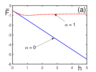
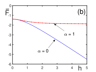
Figure 1: Yes-no model with regulation cost. Behavior of the free energy $F$ as a function of the regulation force $h$ for different temperatures (noise intensity), when $T<1$ in Fig. 1a and when $T>1$ in Fig. 1b.

     

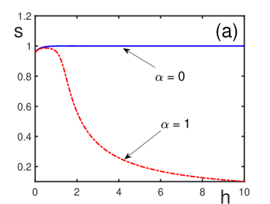
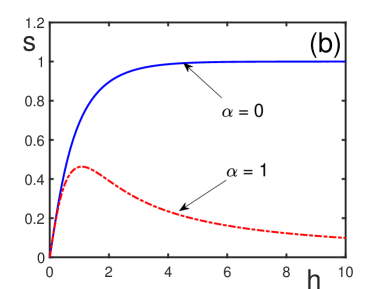
Figure 2: Yes-no model with regulation cost. Order parameter $s$ as a function of the regulation force $h$ for different temperatures, low $(T<1)$ and high $(T>1)$.

3.9 Fluctuating Groups

It is the usual situation when the society members separate into several groups with different properties, so that the number of members in a group is not constant but varies with time. For example, these could be the groups of opponents to the government, workers on strike, opposition organizations, and like that. Different groups of agents can be described by different order parameters. The groups can be localized in some spatial parts of the society or may move through the whole society space. The groups are not permanent in their agent numbers and do not necessarily exist forever, but they can arise and vanish. In that sense, the groups are fluctuating: They can appear, change, and then disappear.

Let the number of agents in a fluctuating group be $N_{f}$ and the characteristic time during which they do not essentially change be $t_{f}$ . Fluctuating groups are mesoscopic, at least in one of the following senses.

Mesoscopic in size:

$$1\ll N_{f}\ll N\;.$$ (3.89)

The number $N_{f}$ is much larger than one for the group order parameter to be defined. And $N_{f}$ is much smaller than the total number of agents N in the society to be classified as a group inside that society.

Mesoscopic in time:

$$t_{int}\ll t_{f}\ll t_{exp}\;,$$ (3.90)

where $t_{int}$ is the characteristic interaction time between the agents and $t_{exp}$ is the observation (experiment) time during which the society is studied. The time $t_{f}$ has to be much larger than the interaction time in order that the groups as such could be formed. And $t_{f}$ is much smaller than the observation time for the groups to be classified as fluctuating. The general method of describing this kind of a society containing fluctuating groups is presented in this section.

Let us consider a snapshot of a society picture, where the spatial location of a $j$-th agent of a society is denoted by a vector ${\bf a}_{j}$. The overall society containing all its members is given by the collection

$$\mathbb{G}=\left\{{\bf a}_{j}:~{}j=1,2,\ldots,N\right\}\;.$$ (3.91)

The society consists of several groups, each being characterized by its specific feature. The features are enumerated by the index $f=1,2,\ldots$. A group with an $f$-th feature is

$$\mathbb{G}_{f}=\left\{{\bf a}_{j}\in\mathbb{G}_{f}:~{}j=1,2,\ldots,N_{f}\right\}\;.$$ (3.92)

The union of all groups forms the whole society

$$\bigcup_{f}\;\mathbb{G}_{f}=\mathbb{G}\;,\qquad\sum_{f}N_{f}=N\;.$$ (3.93)

The spatial locations of groups is represented by the manifold indicator functions

$$\xi_{f}({\bf a}_{j})=\left\{\begin{array}[]{ll}1\;,{}&~{}{\bf a}_{j}\in\mathbb{G}_{f}\\ 0\;,{}&~{}{\bf a}_{j}\not\in\mathbb{G}_{f}\end{array}\right.\;.$$ (3.96)

The collection of all indicator functions, showing the society configuration, is denoted as

$$\xi=\{\xi_{f}({\bf a}_{j}):~{}{\bf a}_{j}\in\mathbb{G}\;,~{}f=1,2,\ldots\}\;.$$ (3.97)

The indicator functions possess the properties

$$\sum_{f}\xi_{f}({\bf a}_{j})=1\;,\qquad\sum_{j}\xi_{f}({\bf a}_{j})=N_{f}\;,$$ (3.98)

the first of which means that each agent pertains to some of the groups, while the second shows the number of agents in an $f$-th group.

In a realistic society, the agents can change their locations, so that the location vector ${\bf a}_{j}={\bf a}_{j}(t)$ depends on time $t$. Hence the society configuration also is a function of time,

$$\xi(t)=\{\xi_{f}({\bf a}_{j}(t)):~{}{\bf a}_{j}(t)\in\mathbb{G}\;;~{}f=1,2,\ldots\}\;.$$ (3.99)

Since $t_{exp}\gg t_{int}$, the observable quantities describing the society correspond to the double average, over the system variables and over time,

$$\langle\;A(\sigma,\xi(t))\;\rangle=\sum_{\sigma}\frac{1}{t_{exp}}\;\int_{0}^{t_{exp}}\rho(\sigma,\xi(t))A(\sigma,\xi(t))\;dt\;.$$ (3.100)

The motion of the groups inside the society usually is so much complicated that it is neither possible nor reasonable to follow the detailed movements of all agents, but the agent locations can be treated as random. Then it is possible to interchange the averaging over time with the averaging over the random society configurations by the rule

$$\frac{1}{t_{exp}}\;\int_{0}^{t_{exp}}dt\longmapsto\int{\cal D}\xi\;.$$ (3.101)

Then we need to realize the functional integration over the manifold indicator functions. We will not describe the mathematical details of the integration that can be found in review articles [47, 48], but will present the results.

The probability distribution $\rho(\sigma,\xi)$ of a heterophase society, depending on the configuration $\xi$, can be derived following Sec. 2.2. The probability is to be normalized,

$$\sum_{\sigma}\int\rho(\sigma,\xi)\;{\cal D}\xi=1\;.$$ (3.102)

The average energy is given by the expression

$$\sum_{\sigma}\int\rho(\sigma,\xi)H(\sigma,\xi)\;{\cal D}\xi=E\;.$$ (3.103)

The information functional takes the form

$$I[\;\rho(\sigma,\xi)\;]=\sum_{\sigma}\int\rho(\sigma,\xi)\;\ln\;\frac{\rho(\sigma,\xi)}{\rho_{0}(\sigma,\xi)}\;{\cal D}\xi\;+$$

$$+\;\lambda_{0}\left[\;\sum_{\sigma}\int\rho(\sigma,\xi)\;{\cal D}\xi-1\;\right]+\lambda\left[\;\sum_{\sigma}\int\rho(\sigma,\xi)\;H(\sigma,\xi)\;{\cal D}\xi-E\;\right]\;.$$ (3.104)

Minimizing the information functional and assuming the uniformity of the trial distribution $\rho_{0}(\sigma,\xi)=const$ yields the probability

$$\rho(\sigma,\xi)=\frac{1}{Z}\;e^{-\beta H(\sigma,\xi)}\;,$$ (3.105)

with the partition function

$$Z=\sum_{\sigma}\int e^{-\beta H(\sigma,\xi)}\;{\cal D}\xi\;.$$ (3.106)

The free energy reads as

$$F=-T\ln Z=-T\ln\sum_{\sigma}\int e^{-\beta H(\sigma,\xi)}\;{\cal D}\xi\;.$$ (3.107)

Observable quantities are given by the averages

$$\langle\;A(\sigma,\xi)\;\rangle=\sum_{\sigma}\int\rho(\sigma,\xi)A(\sigma,\xi)\;{\cal D}\xi\;.$$ (3.108)

Accomplishing the averaging over configurations allows us to define an effective Hamiltonian $\widetilde{H}$ by the relation

$$e^{-\beta\widetilde{H}}=\int e^{-\beta H(\sigma,\xi)}\;{\cal D}\xi\;.$$ (3.109)

The effective Hamiltonian takes the form

$$\widetilde{H}=\bigoplus_{f}\;H_{f}\;,\qquad H_{f}=H_{f}(\sigma,w_{f})\;,$$ (3.110)

in which the probability that an agent pertains to a $j$-th group is

$$w_{f}\equiv\frac{N_{f}}{N}\;.$$ (3.111)

In other words, this is the fraction of the society agents belonging to the $f$-th group. Of course, the normalization conditions are valid,

$$\sum_{f}w_{f}=1\;,\qquad 0\leq w_{f}\leq 1\;.$$ (3.112)

The group probabilities are the minimizers of the free energy

$$F=-T\ln\sum_{\sigma}e^{-\beta\widetilde{H}}\;,$$ (3.113)

under the normalization conditions (3.112),

$$F={\rm abs}\min F(w_{1},w_{2},\ldots)\;.$$ (3.114)

The observable quantities are given by the averages

$$\langle\;A(\sigma,\xi)\;\rangle=\sum_{f}\langle\;A_{f}(\sigma,w_{f})\;\rangle\;,$$ (3.115)

where

$$\langle\;A_{f}(\sigma,w_{f})\;\rangle=\sum_{\sigma}\rho_{f}(\sigma,w_{f})A_{f}(\sigma,w_{f})\;,$$ (3.116)

with the effective probability distributions

$$\rho_{f}(\sigma,w_{f})=\frac{1}{Z_{f}}\;e^{-\beta H_{f}(\sigma,w_{f})}\;,$$ (3.117)

and the partition functions

$$Z_{f}=\sum_{\sigma}e^{-\beta H_{f}(\sigma,w_{f})}\;.$$ (3.118)

The sum of direct summation $\bigoplus$ in Eq. (3.110) is used instead of the simple sum in order to stress that the summands are defined on different configuration sets

$$X_{f}=\{\sigma_{fj}:~{}j=1,2,\ldots,N_{f}\}\;,$$ (3.119)

with the total society configuration set being the tensor product

$$X=\bigotimes_{f}\;X_{f}\;.$$ (3.120)

This is the general approach for describing the heterophase societies with fluctuating groups. The approach reduces the consideration of quasi-equilibrium systems with mesoscopic group fluctuations to the description of effective equilibrium systems with a renormalized effective Hamiltonian. The mathematics of accomplishing functional integration over manifold indicator functions is described in reviews [21, 47, 48]. More mathematical details are presented in Refs. [49, 50, 51]. In the following section, we give an example of applying this approach.

3.10 Self-Organized Disorder

Let us consider the yes-no model of Sec. 3.5 modified so that to take account of fluctuating groups. For simplicity, we shall keep in mind two groups, one called ordered and the other disordered. The ordered group consists of agents agreeing with each other and characterized by a nonzero order parameter, while the disordered group is described by a zero order parameter to be defined below.

Each $j$-th agent from an $f$-th group is characterized by the features $\sigma_{fj}$. In the yes-no model, these features are described by the variable $\sigma_{fj}=\pm 1$. The total feature set for the whole system is the configuration set (3.120).

In addition to the interaction $J_{ij}>0$, typical for self-organization in the yes-no model, we need to include other interactions that would describe some disagreements between the agents. We denote the disordering interaction by $U_{ij}$.

In the snapshot picture, the Hamiltonian with ordering and disordering interactions reads as

$$H(\sigma,\xi)=H_{1}(\sigma,\xi_{1})\bigoplus H_{2}(\sigma,\xi_{2})\;,$$ (3.121)

with

$$H_{f}(\sigma,\xi_{f})=\frac{1}{2}\sum_{i\neq j}^{N}\xi_{f}({\bf a}_{i})\xi_{f}({\bf a}_{j})U_{ij}-\;\frac{1}{2}\sum_{i\neq j}^{N}\xi_{f}({\bf a}_{i})\xi_{f}({\bf a}_{j})J_{ij}\sigma_{fi}\sigma_{fj}\;.$$ (3.122)

Here the manifold indicator functions show the belonging of the agents to the corresponding groups.

After averaging over group configurations, we obtain the effective Hamiltonian

$$\widetilde{H}=H_{1}\bigoplus H_{2}\;,\qquad H_{f}=H_{f}(\sigma,w_{f})\;,$$

$$H_{f}(\sigma,w_{f})=\frac{1}{2}\;w_{f}^{2}\sum_{i\neq j}^{N}(U_{ij}-J_{ij}\sigma_{fi}\sigma_{fj})\;.$$ (3.123)

The order parameter for the $f$-th group is

$$s_{f}\equiv\frac{1}{N}\sum_{j=1}^{N}\langle\;\sigma_{fj}\;\rangle\;,$$ (3.124)

which translates into the equation

$$s_{f}=\tanh\left(\frac{Jw_{f}^{2}s_{f}}{T}\right)\;.$$ (3.125)

Let the first group be ordered, so that

$$s_{1}\neq 0\;,$$ (3.126)

while the second group be disordered in the sense that

$$s_{2}\equiv 0\;.$$ (3.127)

In the case of two groups, it is convenient to denote the fraction of agents in the ordered group and disordered group as

$$w_{1}\equiv w\;,\qquad w_{2}=1-w\;.$$ (3.128)

Then the necessary condition for the free-energy minimum is

$$\frac{\partial F}{\partial w}=\left\langle\;\frac{\partial\widetilde{H}}{\partial w}\;\right\rangle=0\;.$$ (3.129)

This results in the equation

$$w=\frac{u-s_{2}^{2}}{2u-s_{1}^{2}-s_{2}^{2}}\;,$$ (3.130)

in which the notation is used:

$$u\equiv\frac{U}{J}\;,\qquad U\equiv\frac{1}{N}\sum_{i\neq j}^{N}U_{ij}\;,\qquad J\equiv\frac{1}{N}\sum_{i\neq j}^{N}J_{ij}\;.$$ (3.131)

Taking into account that the disordered group is described by the zero order parameter $s_{2}=0$, we have the fraction of agents in the ordered group

$$w=\frac{u}{2u-s_{1}^{2}}\;.$$ (3.132)

Due to the probability definition $0\leq w\leq 1$, and because $0\leq s_{1}\leq 1$, expression (3.132) exists only for sufficiently strong disordering interactions, such that $u\geq 1$.

Note that the second derivative of the free energy, to be positive, leads to the inequality

$$\frac{\partial^{2}F}{\partial w^{2}}=\left[\left\langle\frac{\partial^{2}\widetilde{H}}{\partial w^{2}}\right\rangle\;-\;\beta\left\langle\left(\frac{\partial\widetilde{H}}{\partial w}\right)^{2}\right\rangle\right]~{}>~{}0\;,$$ (3.133)

which yields the condition $u>1/2$.

The society reduced energy

$$\overline{E}\equiv\frac{\langle\widetilde{H}\rangle}{JN}$$ (3.134)

leads to

$$\overline{E}=\overline{E}_{1}+\overline{E}_{2}\;,\qquad E_{f}=\frac{1}{2}\;w_{f}^{2}\left(u-s_{f}^{2}\right)\;.$$ (3.135)

For simplicity, let us study the case of no noise, so that $T=0$. Then $s_{1}=1$ and the energy becomes

$$\overline{E}=w^{2}\left(u-\;\frac{1}{2}\right)+\left(\frac{1}{2}-w\right)u\;,$$ (3.136)

while the fraction of ordered agents is

$$w=\frac{u}{2u-1}\;.$$ (3.137)

Thus the society energy is

$$\overline{E}=\frac{u(u-1)}{2(2u-1)}\;.$$ (3.138)

Now we have to decide what society is more stable, that which contains fluctuating disordered groups or that one which does not contain them? The more stable is that society whose free energy is lower. In the case of very small noise, we need to compare the corresponding expected energies.

If no fluctuating groups would be allowed, then the ordered fraction would be exactly one $(w\equiv 1)$. The energy of a completely ordered society is

$$E_{ord}\equiv\overline{E}(w=1)=\frac{u-1}{2}\;,$$ (3.139)

where $w\equiv 1$. If the whole society would contain only disordered agents $(w\equiv 0)$, then the society energy would be

$$E_{dis}\equiv\overline{E}(w=0)=\frac{1}{2}\;u\;.$$ (3.140)

The society with disorder group fluctuations is more stable, when its energy is lower. Comparing the above expressions we see that

$$\overline{E}<E_{ord}<E_{dis}\qquad(u>1)\;.$$ (3.141)

Thus, for competing interactions, satisfying the condition $u>1$, the energy of the society with fluctuating disorder is lower than that for the perfectly ordered society that, in turn, is lower than the disordered society. That is, a completely ordered society is more stable than a disordered society. However the most stable is a society with the admixture of fluctuating disorder. Thus disorder fluctuations make the society more stable. In that sense the disorder is self-organized.

The total order parameter is defined as the average of the expression

$$M(\sigma,\xi)=\frac{1}{N}\sum_{f}\sum_{j=1}^{N}\xi_{f}({\bf a}_{j})\sigma_{fj}\;,$$ (3.142)

which gives

$$M=\langle\;M(\sigma,\xi)\;\rangle=\sum_{f}w_{f}s_{f}\;.$$ (3.143)

When there is no noise, that is at zero temperature, we get

$$M=ws_{1}=\frac{u}{2u-1}\qquad(T=0)\;.$$ (3.144)

Concluding, under sufficiently strong competition between the society agents, there spontaneously appear social disorder groups. When the disorder groups appear, they diminish the total society order. However, the existence of the disorder groups makes the society more stable. This is an example showing that it is not always useful to try to realize a complete order in a society, since the presence of some disorder can make the society more stable. Sometimes societies for being more stable generate self-organized disorder.

3.11 Coexistence of Populations

Very often social systems consist of several groups of rather different people, so that the groups are more or less stable and on average do not essentially change for long time, contrary to fluctuating groups considered in the previous section. Each of the groups can be characterized by different typical agents. There exist numerous examples of such societies. Thus a society, forming a country, very often can include groups having different nationality or religion.

In a society composing a financial market, there are the groups of fundamentalists and chartists. Fundamentalists base their decisions upon market fundamentals, such as interest rates, growth or decline of the economy, company’s performance, etc. Fundamentalists expect the asset prices to move towards their fundamental values, hence, they either buy or sell assets that are assumed to be undervalued or, respectively, overvalued. Chartists, or technical analysts, look for patterns and trends in the past market prices and base their decisions upon extrapolation of these patterns. There exist as well the groups of contrarians who buy or sell contrary to the trend followed by the majority.

Different groups of people or other alive beings, having differing features, are called populations. Let a society, inhabiting the volume $V$, contain several different populations enumerated by the index $n=1,2,\ldots$. In an $n$-th population, there are $N_{n}$ members. In what follows, we consider a general approach describing whether the populations can or cannot coexist with each other. The populations can be of any origin. For concreteness, we can keep in mind different population groups living in a country.

The populations can either peacefully live in the whole country, which can be called a mixed society, or can possess the tendency of separating from each other, thus having no intention for joint coexistence. Our aim is to understand how we could quantify the conditions when different populations prefer to live together and when they wish to separate.

According to the general law, that society is more stable whose free energy is lower. That is, a mixed society, living in the same country, is more stable than the separated populations, existing separately from each other, if the free energy $F_{mix}$ of the mixed society is lower that the free energy $F_{sep}$ of the separated society,

$$F_{mix}<F_{sep}\;.$$ (3.145)

The free energies can be represented as

$$F_{mix}=E_{mix}-TS_{mix}\;,\qquad F_{sep}=E_{sep}-TS_{sep}\;.$$ (3.146)

Therefore, denoting the entropy of mixing

$$\Delta S_{mix}\equiv\frac{1}{N}\;(S_{mix}-S_{sep})\;,$$ (3.147)

we have the condition of stability of the united country:

$$E_{mix}-E_{sep}<NT\Delta S_{mix}\;.$$ (3.148)

We need to write down the energy of the mixed and separated populations. For this purpose, let us denote the density of an $n$-th population by $\rho_{n}({\bf r})$ and the interaction between the members of an $m$-th and $n$-th populations by $\Phi_{mn}({\bf r})$. Then the interaction energy for the mixed populations can be represented as

$$E_{mix}=\frac{1}{2}\sum_{mn}\int_{V}\rho_{m}({\bf r})\;\Phi_{mn}({\bf r}-{\bf r}^{\prime})\;\rho_{n}({\bf r}^{\prime})\;d{\bf r}d{\bf r}^{\prime}\;.$$ (3.149)

Assuming a uniform distribution of the people across the country implies the unform densities

$$\rho_{m}({\bf r})=\frac{N_{m}}{V}\;,\qquad\rho_{n}({\bf r})=\frac{N_{n}}{V}\;.$$ (3.150)

Thus the interaction energy of a country with mixed populations reads as

$$E_{mix}=\frac{1}{2}\sum_{mn}\Phi_{mn}\;\frac{N_{m}N_{n}}{V}\;,$$ (3.151)

where the quantity

$$\Phi_{mn}\equiv\int_{V}\Phi_{mn}({\bf r})\;d{\bf r}$$ (3.152)

describes the average interaction strength between the members of an $m$-th and $n$-th populations.

Now let us consider the case of separated populations, when each population lives in its separate location characterized by the volume $V_{n}$. Then the energy of a separated country is the sum

$$E_{sep}=\frac{1}{2}\sum_{n}\int_{V_{n}}\rho_{n}^{sep}({\bf r})\;\Phi_{nn}({\bf r}-{\bf r}^{\prime})\;\rho_{n}^{sep}({\bf r}^{\prime})\;d{\bf r}d{\bf r}^{\prime}\;.$$ (3.153)

Keeping again in mind that each population inside their part of the country is uniformly distributed gives the uniform densities

$$\rho_{n}^{sep}({\bf r})=\frac{N_{n}}{V_{n}}\;.$$ (3.154)

Then the energy of a separated country is

$$E_{sep}=\frac{1}{2}\sum_{n}\overline{\Phi}_{nn}\;\frac{N_{n}^{2}}{V_{n}}\;,$$ (3.155)

where

$$\overline{\Phi}_{nn}\equiv\int_{V_{n}}\Phi_{nn}({\bf r})\;d{\bf r}\;.$$ (3.156)

Using the identity

$$\frac{V}{V_{m}}=\sum_{n}\frac{V_{m}}{V_{n}}$$

reduces the energy of a separated country to

$$E_{sep}=\frac{1}{2}\sum_{mn}\overline{\Phi}_{mm}\;\frac{N_{m}^{2}N_{n}}{VV_{m}}\;.$$ (3.157)

Any two different populations, though being separated, exercise pressure on each other through their common boundary. If the pressure of one of them is larger than that of another, there is no equilibrium between the populations, but there can arise nonequilibrium movements, such as invasions and wars. The equilibrium coexistence of two separated populations implies the equality of their pressures:

$$P_{m}=P_{n}\qquad\left(P_{n}=-\;\frac{\partial F_{sep}}{\partial V_{n}}\right)\;.$$ (3.158)

By its meaning, this equality can be called no-war condition. For not too strong noise, such that

$$\frac{\partial F_{sep}}{\partial V_{m}}\;\cong\;\frac{\partial E_{sep}}{\partial V_{m}}=\frac{1}{2}\;\overline{\Phi}_{mm}\left(\frac{N_{m}}{V_{m}}\right)^{2}\;,$$

we find the no-war condition in the form

$$\frac{\overline{\Phi}_{mm}}{\overline{\Phi}_{nn}}=\left(\frac{N_{n}V_{m}}{N_{m}V_{n}}\right)^{2}\;.$$ (3.159)

This shows that two neighboring populations have no war, being in equilibrium with each other, only when the signs of the effective interactions of the members inside each population are the same and the interactions satisfy the above conditions. An $m$-th population and $n$-th population can be in equilibrium, only when their internal interactions $\Phi_{mm}$ and $\Phi_{nn}$ are both either positive or negative. If for one population $\Phi_{mm}>0$, while for the members of another population $\Phi_{nn}<0$, then there can be no equilibrium between such neighboring populations.

Taking account of the no-war condition (3.159) makes it possible to rewrite the energy of the separated country in the form

$$E_{sep}=\frac{1}{2}\sum_{mn}\frac{N_{m}N_{n}}{V}\;\sqrt{\overline{\Phi}_{mm}\overline{\Phi}_{nn}}\;.$$ (3.160)

Then the condition of stability (3.148) for the mixed society yields the inequality

$$\sum_{mn}\frac{N_{m}N_{n}}{2V}\;\left(\Phi_{mn}-\;\sqrt{\overline{\Phi}_{mm}\overline{\Phi}_{nn}}\;\right)~{}<~{}NT\Delta S_{mix}\;.$$ (3.161)

With the identity

$$N\equiv\frac{1}{N}\sum_{mn}N_{m}N_{n}\;,$$

we find

$$\sum_{mn}\;\frac{N_{m}N_{n}}{2V}\left(\Phi_{mn}-\;\sqrt{\overline{\Phi}_{mm}\overline{\Phi}_{nn}}\;-\;\frac{2T}{\rho}\;\Delta S_{mix}\right)~{}<~{}0\;,$$ (3.162)

where $\rho=N/V$ is the average density of the total population. From here, the sufficient condition of stability for the mixed country becomes

$$\Phi_{mn}~{}<~{}\sqrt{\overline{\Phi}_{mm}\overline{\Phi}_{nn}}\;+\;\frac{2T}{\rho}\;\Delta S_{mix}\;.$$ (3.163)

The entropy of mixture can be represented as

$$\Delta S_{mix}=-\sum_{m}n_{m}\ln n_{m}\qquad\left(n_{m}\equiv\frac{N_{m}}{N}\right)\;.$$ (3.164)

Thus we obtain the condition of stability for the country with mixed population, as compared to the country where the populations are separated,

$$\Phi_{mn}\;-\;\sqrt{\overline{\Phi}_{mm}\overline{\Phi}_{nn}}~{}<~{}-\;\frac{2T}{\rho}\sum_{m}n_{m}\ln n_{m}\;.$$ (3.165)

When this condition is not valid, the country with mixed population is not stable and it will disintegrate into several separate countries, each being composed of just one population type. There exist numerous examples of countries that have disintegrated into several smaller countries. This destiny, e.g., has happened with the Roman Empire, Makedonsky Empire, British Empire, French Empire, Austrian Empire, Ottoman Empire, Soviet Union, Yugoslavia, and Czechoslovakia.

3.12 Forced Coexistence

From the history we know that empires are usually kept united not merely by economical advantage of the countries composing them by also by force. Why this is possible and what happens when the required force becomes too strong? Is it possible to keep together different populations inside one empire by increasing force? To answer these questions, it is necessary to consider the case with imposed regulations, including regulation cost.

Let the regulation force, acting on a member of an $n$-th population be $f_{n}({\bf r})$. The energy of a society with mixed populations, including the force applied for keeping different populations together, can be written as

$$E_{mix}=\frac{1}{2}\sum_{mn}\int_{V}\rho_{m}({\bf r})\;\Phi_{mn}({\bf r}-{\bf r}^{\prime})\;\rho_{n}({\bf r}^{\prime})\;d{\bf r}d{\bf r}^{\prime}-\sum_{n}\int_{V}f_{n}({\bf r})\;\rho_{n}({\bf r})\;d{\bf r}+$$

$$+\frac{1}{2}\sum_{mn}\int_{V}\rho_{m}({\bf r})\;f_{m}({\bf r})\;A_{mn}({\bf r}-{\bf r}^{\prime})\;f_{n}({\bf r}^{\prime})\;\rho_{n}({\bf r}^{\prime})\;d{\bf r}d{\bf r}^{\prime}\;,$$ (3.166)

where the last term characterizes the cost of supporting the regulation force, with $A_{mn}({\bf r})$ being the strength of the interaction between the members of the society caused by the applied force at each other.

It is possible to assume that the population densities are uniform and the force is constant, so that

$$\rho_{n}({\bf r})=\frac{N_{n}}{V}\;,\qquad f_{n}({\bf r})=f_{n}\;.$$ (3.167)

Then the society energy reads as

$$E_{mix}=\frac{1}{2}\sum_{mn}(\Phi_{mn}+A_{mn}f_{m}f_{n})\;\frac{N_{m}N_{n}}{V}-\sum_{n}f_{n}N_{n}\;,$$ (3.168)

where

$$A_{mn}\equiv\int_{V}A_{mn}({\bf r})\;d{\bf r}\;.$$ (3.169)

When the society is disintegrated into several independent countries, there is no need to apply force, hence the energy of a society with separated populations is (3.160). Using the identity

$$\sum_{n}f_{n}N_{n}=\frac{1}{2N}\sum_{mn}N_{m}N_{n}(f_{m}+f_{n})$$

and following the same way as in the previous section, we obtain the sufficient condition for the society with mixed populations

$$\Phi_{mn}+A_{mn}f_{m}f_{n}~{}<~{}\sqrt{\overline{\Phi}_{mm}\overline{\Phi}_{nn}}\;+\;\frac{2}{\rho}\left(T\Delta S_{mix}+\frac{f_{m}+f_{n}}{2}\right)\;.$$ (3.170)

For short, this condition can be named the condition of empire stability. If it does not hold, the empire disintegrates into separate countries.

Condition (3.170) shows that switching on the regulating force, first, increases the right-hand side of the inequality, thus making the mixed society more stable. However, too strong force makes the left-hand side of the inequality larger, thus leading to the instability of the empire and its disintegration. Hence, by enforcing reasonable regulations, it is possible to keep the coexistence of populations, even when without such an enforcement the country would disintegrate. However, the regulating force should not be too strong. This explains why, for some time, an empire can exist as a united family of different populations. But when the enforcement is too costly, it turns unbearable, and disintegration becomes inevitable. Empires do not exist forever.

An empire, with forced coexistence of different populations, is practically always less stable than several independent countries, with their own populations and weaker regulation forces. However the unions of different populations also can exist, when they are kept not by force, but by their collaborative interactions. The prominent example is Switzerland, where the German, French, and Italian cantons peacefully coexist, not being forced, but due to the advantage of their mutual interactions.

4 Collective Decisions in a Society

The models considered above allow us to describe general structures and states of social systems, whose members exhibit specific behavior. Thus in the yes-no model, the members are assumed to take decisions, either “yes” or “no”, with regard to some problem, say voting in elections or buying something. As is evident, the underlying process of any action is the process of taking decisions. It is possible to say that practically all properties of a social system are caused by the decisions taken by its members. This is why it is so important to have general understanding of how decisions are made. In the present chapter, we consider some models describing the way of how the members of a society take decisions. Collective decisions are based on decisions made by individuals interacting with each other. Therefore, first of all it is necessary to understand how decisions are taken by individuals and then to model how they interact between themselves for reaching a collective decision. Moreover, there are deep parallels between the process of making decisions by individuals and by groups, since even individual decision making is a kind of collective decision making accomplished by the neurons of a brain. Since the notions of decision making theory are less known for the physically oriented audience, we give below an overview of the main literature and describe the basic points of the theory.

4.1 General Overview

Nowadays, the dominant theory, describing individual behavior of decision makers is expected utility theory. This theory was introduced by Bernoulli [52], when investigating the so-called St. Petersburg paradox. Von Neumann and Morgenstern [53] axiomatized this theory. Savage [54] integrated within the theory the notion of subjective probability. The power of the theory was demonstrated by Arrow [55], Pratt [56], and by Rothschild and Stiglitz [57, 58] in the studies of risk aversion. The flexibility of the theory for characterizing the attitudes of decision makers toward risk was illustrated by Friedman and Savage [59] and Markowitz [60]. The expected utility theory has provided mathematical basis for several fields of economics, finance, and management, including the theory of games, the theory of investment, and the theory of search [61, 62, 63, 64, 65, 66, 67, 68, 69, 70].

Despite many successful applications of the expected decision theory, quite a number of researchers have discovered a large body of evidence that decision makers, both human as well as animal, often do not obey prescriptions of the theory and depart from this theory in a rather systematic way [71]. Then there appear numerous publications, beginning with Allais [72], Edwards [73, 74], and Ellsberg [75], which experimentally confirmed systematic deviations from the prescriptions of expected utility theory, leading to a number of paradoxes.

As examples of such paradoxes, it is possible to mention the Allais paradox [72], independence paradox [72], Ellsberg paradox [75], Kahneman-Tversky paradox [76], Rabin paradox [77], Ariely paradox [71], disjunction effect [78], conjunction fallacy [79, 80], isolation effects [81], planning paradox [82], and dynamic inconsistency [83, 84].

In order to avoid paradoxes, there have been many attempts to change the expected utility theory, which has been named as non-expected utility theories. There is a number of such non-expected utility theories, among which we mention just a few, the most known approaches. These are prospect theory [73, 76, 85], weighted-utility theory [86, 87, 88], regret theory [89], optimism-pessimism theory [90], dual-utility theory [91], ordinal-independence theory [92], quadratic-probability theory [93]. More detailed information on this topic can be found in the recent reviews by Camerer et al. [94] and Machina [95].

Despite numerous attempts of treating expected utility theory, none of the suggested modifications can explain all those paradoxes, as has been shown by Safra and Sigal [96]. The best that could be achieved is a fitting for interpreting just one or a couple of paradoxes, with other paradoxes remaining unexplained. Moreover, spoiling the structure of expected utility theory results in the appearance of several inconsistences. Accomplishing a detailed analysis, Al-Najjar and Weinstein [97, 98] concluded that any variation of the expected utility theory “ends up creating more paradoxes and inconsistences than it resolves”.

An original interpretation was advanced by Bohr [99, 100, 101], who suggested that psychological processes could be described by resorting to quantum notions, such as interference and complimentarity. Von Neumann [102] mentioned that the theory of quantum measurements could be interpreted as decision theory. These ideas were developed in quantum decision theory [103, 104], on the basis of which the classical decision-making paradoxes could be explained. It has also been shown [105, 106] that quantum decision theory can be reformulated to the classical language employing no quantum formulas.

When decision makers interact with each other, the process of decision making becomes collective [107, 108, 109, 110, 111, 112]. Then each individual takes decisions being based not solely on personal deliberations, but also to some extent imitating the actions of other members of the society. Sometimes, this imitation grows to the level of herding effect. In the present chapter, we describe the main steps of how the process of decision making develops, starting from individual decisions to collective decisions taken by a network of society members.

4.2 Utility Function

The primary elements in a problem of choice are some events, or outcomes, or consequences, or payoffs denoted as $x$. One considers a set of outcomes, or a set of payoffs, or consumer set, or a field of events

$$X=\{x_{i}:i=1,2,\ldots,N\}.$$ (4.1)

Generally, payoffs $x_{i}$ can be either finite or infinite, as well as the payoff set can be finite or infinite. Mathematically correct definition of infinity is through the limit of a sequence.

Payoffs or outcomes have to be measured in a common system of units, accomplished through a utility function $u(x)$, also called elementary utility function, pleasure function, satisfaction function, or profit function $u(x):\quad X\rightarrow\mathbb{R}$. The utility function has to satisfy the following properties:

(i) It has to be nondecreasing, so that

$$u(x_{1})\geq u(x_{2})\qquad(x_{1}\geq x_{2})\;.$$ (4.2)

If (4.2) is a strict inequality, the function is termed strictly increasing.

(ii) It is often (although not always) taken to be concave, when

$$u(\alpha_{1}x_{1}+\alpha_{2}x_{2})\geq\alpha_{1}u(x_{1})+\alpha_{2}u(x_{2}),$$ (4.3)

where

$$\alpha_{1}\geq 0\;,\qquad\alpha_{2}\geq 0\;,\qquad\alpha_{1}+\alpha_{2}=1\;.$$

It is called strictly concave, if (4.3) is a strict inequality.

A twice differentiable function is nondecreasing if

$$u^{\prime}(x)\equiv\frac{du(x)}{dt}\geq 0$$

and it is concave when

$$u^{\prime\prime}(x)\equiv\frac{d^{2}u(x)}{dx^{2}}\leq 0\;.$$

The derivative $u^{\prime}(x)$ defines the marginal utility function. According to the above properties, the marginal utility does not increase.

An important property of a utility function is its risk aversion. The degree of absolute risk aversion is measured [56] by the quantity

$$r(x)\equiv-\;\frac{u^{\prime\prime}(x)}{u^{\prime}(x)}\;.$$ (4.4)

Coefficient of relative risk aversion [55, 56] is defined as

$$\widetilde{r}(x)\equiv xr(x)=-x\;\frac{u^{\prime\prime}(x)}{u^{\prime}(x)}.$$ (4.5)

For a concave utility function, the degree of risk aversion is non-negative, hence utility function is risk averse, $r(x)\geq 0$. This means that with increasing $x$, the growth of the utility function $u(x)$ does not increase.

In practice, one often employs a linear utility function

$$u(x)=kx\qquad(k>0)\;.$$ (4.6)

For this function,

$$u^{\prime}(x)=k\;,\qquad u^{\prime\prime}(x)=0\;,$$

hence the degree of risk aversion is zero, $r(x)=0$.

Another used form is a power-law utility function

$$u(x)=kx^{\gamma}\qquad(k>0,\;0\leq\gamma<1)\;,$$ (4.7)

assuming $x\geq 0$. For this case,

$$u^{\prime}(x)=\frac{k\gamma}{x^{1-\gamma}}\;,\qquad u^{\prime\prime}(x)=-\frac{k\gamma(1-\gamma)}{x^{2-\gamma}}\;.$$

The degree of risk aversion diminishes with increasing $x$ as

$$r(x)=\frac{1-\gamma}{x}>0\;.$$

One more example is the logarithmic utility function

$$u(x)=c\ln(1+kx)\qquad(c>0,\;k>0)\;,$$ (4.8)

again keeping in mind $x\geq 0$. Then

$$u^{\prime}(x)=\frac{ck}{1+kx}\;,\qquad u^{\prime\prime}(x)=-\;\frac{ck^{2}}{(1+kx)^{2}}\;.$$

Hence the degree of risk aversion diminishes with the increasing payoff $x$,

$$r(x)=\frac{ck}{1+kx}\;.$$

Sometimes, one uses an exponential utility function

$$u(x)=c\left(1-e^{-kx}\right)\qquad(c>0,\;k>0)\;,$$ (4.9)

for which

$$u^{\prime}(x)=cke^{-kx}\;,\qquad u^{\prime\prime}(x)=-ck^{2}e^{-kx}\;,$$

and the degree of risk aversion is constant, $r(x)=k$.

In above examples, the utility function is twice-differentiable, such that $u^{\prime}(x)$ and $u^{\prime\prime}(x)$ exist, it is non-decreasing, concave, hence risk averse, it is also non-negative for non-negative $x$, and it is normalized to zero, so that $u(0)=0$, implying that the utility of nothing is zero.

Some of the utility functions exemplified above are defined only for positive payoffs $x>0$. In the case of losses, payoffs are negative. Then one defines different utility functions for gains and losses, say, $u_{g}(x)$ for gains and $u_{l}(x)$ for losses. Of course, these should coincide at zero, so that $u_{g}(0)=u_{l}(0)$.

It is also useful to mention that there are two types of utility, cardinal and ordinal. Cardinal utility can be precisely measured and the magnitude of the measurement is meaningful, similarly how distance is measured in meters, or time in hours, or weight in kilograms. For ordinal utility, not its precise magnitude is important, but the magnitude of the ratios between different utilities is only meaningful.

4.3 Expected Utility

The notion of expected utility was introduced by Bernoulli [52] and axiomatic utility theory was formulated by von Neumann and Morgenstern [53]. The definitions below follow the classical exposition of von Neumann and Morgenstern [53].

One defines a probability measure over the set of payoffs

$$\{p(x_{i})\in[0,1]:\;i=1,2,\ldots,N\}\;,$$ (4.10)

with the probabilities $p(x_{i})$ normalized to one,

$$\sum_{i=1}^{N}p(x_{i})=1\;.$$ (4.11)

The probabilities can be objective, prescribed by a rule [53], or they can be subjective probabilities, evaluated by a decision maker [54].

The probability distribution over a set of payoffs is termed a lottery,

$$L=\{x_{i},p(x_{i}):\;i=1,2,\ldots,N\}\;.$$ (4.12)

A compound lottery is a lottery whose outcomes are other lotteries. For two lotteries

$$L_{1}=\{x_{i},p_{1}(x_{i})\}\;,\qquad L_{2}=\{x_{i},p_{2}(x_{i})\}\;,$$

the compound lottery is the linear combination

$$\alpha_{1}L_{1}+\alpha_{2}L_{2}=\{x_{i},\;\alpha_{1}p_{1}(x_{i})+\alpha_{2}p_{2}(x_{i})\}\;,$$ (4.13)

where

$$\alpha_{1}\geq 0\;,\qquad\alpha_{2}\geq 0\;,\qquad\alpha_{1}+\alpha_{2}=1\;.$$

The lottery mean is the lottery expected value

$$E(L)\equiv\sum_{i=1}^{N}x_{i}p(x_{i})\;.$$ (4.14)

Lottery volatility, lottery spread, or lottery dispersion is the variance

$${\rm var}(L)\equiv\sum_{i=1}^{N}x_{i}^{2}p(x_{i})-E^{2}(L)\;.$$ (4.15)

The lottery volatility or lottery dispersion is a measure of the lottery uncertainty.

Expected utility of a lottery is the functional

$$U(L)\equiv\sum_{i=1}^{N}u(x_{i})p(x_{i})\;.$$ (4.16)

The expected utility is proportional to the lottery mean in the case of a linear utility function. Lotteries are ordered implying the following definitions.

Lotteries $L_{1}$ and $L_{2}$ are indifferent if and only if

$$U(L_{1})=U(L_{2})\qquad(L_{1}=L_{2})\;.$$ (4.17)

A lottery $L_{1}$ is preferred to $L_{2}$ if and only if

$$U(L_{1})>U(L_{2})\qquad(L_{1}>L_{2})\;.$$ (4.18)

A lottery $L_{1}$ is preferred or indifferent to $L_{2}$ if and only if

$$U(L_{1})\geq U(L_{2})\qquad(L_{1}\geq L_{2})\;.$$ (4.19)

Expected utility satisfies the following properties.

(i) Completeness. For any two lotteries $L_{1}$ and $L_{2}$, one of the conditions is valid:

$$L_{1}=L_{2}\;,\quad L_{1}<L_{2}\;,\quad L_{1}>L_{2}\;,\quad L_{1}\leq L_{2}\;,\quad L_{1}\geq L_{2}\;.$$ (4.20)

(ii) Transitivity. For any three lotteries, such that $L_{1}\leq L_{2}$ and $L_{2}\leq L_{3}$, it follows that $L_{1}\leq L_{3}$.

(iii) Continuity. For any three lotteries, ordered so that $L_{1}\leq L_{2}\leq L_{3}$, there exists $\alpha\in[0,1]$ for which

$$L_{2}=\alpha L_{1}+(1-\alpha)L_{3}\;.$$ (4.21)

(iv) Independence. For any $L_{1}\leq L_{2}$ and arbitrary $L_{3}$, there exists $\alpha\in[0,1]$, such that

$$\alpha L_{1}+(1-\alpha)L_{3}\leq\alpha L_{2}+(1-\alpha)L_{3}\;.$$ (4.22)

These properties follow directly from the properties of the utility function described above.

The standard decision-making process proceeds through the following steps. For the same set of payoffs $\{x_{n}:n=1,2,...,N\}$, there exist several lotteries

$$L_{n}=\{x_{i},\;p_{n}(x_{i})\}\qquad(n=1,2,\ldots)\;.$$ (4.23)

Defining the utility function $u(x)$, one calculates the expected lottery utilities $U(L_{n})$. Comparing the values $U(L_{n})$, one selects the largest among them.

A lottery $L^{*}$ is named optimal when it is preferred to all others from the given choice of lotteries. A lottery is optimal if and only if its expected utility is the largest:

$$U(L^{*})\equiv{\rm sup}_{n}U(L_{n})\;.$$ (4.24)

The aim of a decision maker is assumed to choose an optimal lottery maximizing the related expected utility.

4.4 Time Preference

Sometimes people need to compare present goods that are available for use at the present time with future goods that are defined as present expectations of goods becoming available at some date in the future. Time preference is the insight that people prefer present goods to future goods [84, 113].

Mathematical description of the time preference effect can be done as follows. Let us consider at time $t=0$ a lottery

$$L=\{x_{i},\;p(x_{i})\}\qquad(t=0)\;.$$ (4.25)

With a utility function $u(x)$ at time $t=0$, the expected utility of the lottery is

$$U(L)=\sum_{i}u(x_{i})p(x_{i})\qquad(t=0)\;.$$ (4.26)

The lottery, expected at time $t>0$, has the form

$$L(t)=\{x_{i}(t),\;p(x_{i}(t))\}\qquad(t>0)\;.$$ (4.27)

Denoting the utility function at time $t>0$ as $u(x(t),t)$, we have the expected utility of $L(t)$ as

$$U(L(t))=\sum_{i}u(x_{i}(t),t)p(x_{i}(t))\;.$$ (4.28)

According to the meaning of time preference, the same goods at future time are valued lower then at the present time just because any goods can be used during the interval of time $[0,t]$. In the case of money, its value increases with time since it can bring additional profit through an interest rate, hence the utility of a fixed amount of money decreases with time. This can be formalized as the inequality

$$u(x_{i},t)<u(x_{i})\qquad(t>0)\;.$$ (4.29)

It is possible to introduce a discount function $D(x,t)$ by the relation

$$u(x_{i},t)=u(x_{i})D(x_{i},t)\;,$$ (4.30)

with the evident condition

$$D(x_{i},0)=1\;.$$ (4.31)

From the time preference condition (4.29), we have

$$D(x_{i},t)<1\qquad(t>0)\;.$$ (4.32)

In this way, if the payoffs at the present time $t=0$ and at a future time $t>0$ are the same, then the present lottery is preferable over the future one,

$$U(L(t))<U(L)\qquad(x_{i}(t)=x_{i})\;.$$ (4.33)

In particular, if the discount function is uniform with respect to the payoffs,

$$D(x_{i},t)=D(t)\;,$$ (4.34)

then

$$U(L(t))=U(L)D(t)\;,$$ (4.35)

where $D(0)=1$.

In decision making, one uses the following discount functions.

Power-law discount function

$$D(t)=\frac{1}{(1+r)^{t}}\;.$$ (4.36)

Exponential discount function

$$D(t)=\exp(-\gamma t)\;.$$ (4.37)

Note that the power-law discount function (4.36) is equivalent to the exponential form (4.37), since they are related by the reparametrization

$$1+r=e^{\gamma}\;,\qquad\gamma=\ln(1+r)\;.$$

Hyperbolic discount function

$$D(t)=\frac{1}{(1+t/\tau)^{\gamma\tau}}\;,$$ (4.38)

with positive parameters $\gamma$ and $\tau$.

A detailed review on the effect of time preference is given in [84].

4.5 Stochastic Utility

There exists a number of factors that influence decision making. These factors are random, or stochastic, because of which the related approach in decision making is named stochastic. These factors, for instance, are:

(i) External conditions under which the decision is made, such as weather, situation in the country, relations with people, opinions of other people, …

(ii) Internal physical state of the decision maker, such as fatigue, illness, pain, influence of alcohol, …

(iii) Internal psychological state, including biases, emotions, mood, impatience, …

(iv) Previous experience, information, prejudices, religion, principles, character, …

(v) Occasional errors in deciding.

Stochastic decision theory assumes that all these interrelated factors can be characterized by some variables, say $\xi$, called states of nature. The total collection of the states of nature forms the nature set $\{\xi\}$. The variables $\xi$ are random, stochastic. It is supposed that there should be given a probability measure $\mu(\xi)$ on the nature set $\{\xi\}$. Utility function $u(x,\xi)$ becomes a random variable. Probability of payoffs $p(x,\xi)$ is also a random variable.

In that way, a lottery becomes a stochastic lottery

$$L(\xi)=\{x_{i},\;p(x_{i},\xi):\;\;i=1,2,\ldots,N\}\;.$$ (4.39)

Respectively, we come to a stochastic utility

$$U(L,\xi)=\sum_{i=1}^{N}u(x_{i},\xi)p(x_{i},\xi)\;.$$ (4.40)

As far as the states on nature are random, one needs to average over these states, thus coming to the expected utility

$$U(L)\equiv\int U(L,\xi)\;d\mu(\xi)\;.$$ (4.41)

The process of stochastic decision making consists in the choice between several stochastic lotteries

$$L_{n}(\xi)=\{x_{i},\;p_{n}(x_{i},\xi):\;\;i=1,2,\ldots,N\}\;.$$ (4.42)

Technically, this implies the choice between several expected utilities

$$U(L_{n})=\int U(L_{n},\xi)\;d\mu(\xi)\;.$$ (4.43)

One needs to choose a lottery with the largest expected utility $U(L^{*})$. This approach, however, confronts several serious difficulties.

(i) It is not clear how the random variables should be incorporated into lotteries.

(ii) Calculations become rather complicated.

(iii) The nature set is not fixed, generally, depending on time.

(iv) The nature set also can depend on the set of payoffs.

(v) The explicit form of the nature states probability is not known and has to be postulated.

More details on stochastic utility theory can be found, e.g., in the books, [114, 115].

4.6 Affective Decisions

People make decisions being based not merely on rational grounds, by calculating utility, but also being affected by emotions that are irrational. Several attempts have been made to take account of emotions in decision making by modifying expected utility, which is equivalent to some variants of non-expected utility models [91, 116, 117]. Here we present the main points of a probabilistic approach of taking into account emotions. First, this approach was formulated by resorting to techniques of quantum theory [103, 104], however later it was shown [105, 106] that it can be reformulated in classical terms, without invoking any quantum expressions. The basics of the probabilistic affective decision theory are as follows.

The aim of any decision making is to choose an alternative from a set of several alternatives. Let the set of alternatives be denoted as

$$\mathbb{A}=\{A_{n}:\;n=1,2,\ldots,N_{A}\}\;.$$ (4.44)

Each alternative from this set is assumed to be equipped with a probability $p(A_{n})$, with the normalization condition

$$\sum_{n}p(A_{n})=1\;,\qquad 0\leq p(A_{n})\leq 1\;.$$ (4.45)

This probability shows how it is probable that the alternative $A_{n}$ can be chosen.

An alternative $A_{1}$ is said to be stochastically preferable to $A_{2}$, if and only if

$$p(A_{1})>p(A_{2})\;.$$ (4.46)

Two alternatives are called stochastically indifferent, if and only if

$$p(A_{1})=p(A_{2})\;.$$ (4.47)

An alternative $A_{opt}$ is stochastically optimal if its probability is maximal,

$$p(A_{opt})=\sup_{n}p(A_{n})\;.$$ (4.48)

The usefulness of an alternative is characterized by a utility factor $f(A_{n})$, whose form is to be prescribed by normative rules. This factor shows the probability of choosing an alternative $A_{n}$ being based on rational understanding of its utility. The standard probability normalization is applied:

$$\sum_{n}f(A_{n})=1\;,\qquad 0\leq f(A_{n})\leq 1\;.$$ (4.49)

One says that an alternative $A_{1}$ is more useful than $A_{2}$, if and only if

$$f(A_{1})>f(A_{2})\;.$$ (4.50)

Two alternatives are equally useful, if and only if

$$f(A_{1})=f(A_{2})\;.$$ (4.51)

Affective features of an alternative are represented by an attraction factor $q(A_{n})$, with the normalization

$$\sum_{n}q(A_{n})=0\;,\qquad-1\leq q(A_{n})\leq 1\;.$$ (4.52)

Positive attraction factors imply attractive alternatives, while negative attraction factors mean that the corresponding alternatives are repulsive. An alternative $A_{1}$ is more attractive than $A_{2}$, if and only if

$$q(A_{1})>q(A_{2})\;.$$ (4.53)

Two alternatives are equally attractive, if and only if

$$q(A_{1})=q(A_{2})\;.$$ (4.54)

The probability $p(A_{n})$ of an alternative $A_{n}$ is a functional of the related utility factor $f(A_{n})$ and of attraction factor $q(A_{n})$, such that the rational boundary condition be valid,

$$p(A_{n})=f(A_{n})\;,\qquad q(A_{n})=0\;,$$ (4.55)

when, in the absence of emotions, the probability of an alternative coincides with the rational utility factor.

The simplest form of the probability functional satisfying the rational boundary condition (4.55) is prescribed by the superposition axiom

$$p(A_{n})=f(A_{n})+q(A_{n})\;.$$ (4.56)

An explicit expression for the utility factor can be derived from the principle of minimal information of Sec. 2. Assume that for each alternative $A_{n}$ there exists a utility functional $U(A_{n})$, so that an average utility is given by the standard condition

$$\sum_{n}f(A_{n})U(A_{n})=U\;.$$ (4.57)

Then the information functional, under conditions (4.49) and (4.57), reads as

$$I[\;f(A_{n})\;]=\sum_{n}f(A_{n})\;\ln\;\frac{f(A_{n})}{f_{0}(A_{n})}+\alpha\left[\;1-\sum_{n}f(A_{n})\;\right]+\beta\left[\;U-\sum_{n}f(A_{n})U(A_{n})\;\right]\;,$$ (4.58)

where $f_{0}(A_{n})$ is a trial distribution. Minimizing the information functional with respect to the utility factor $f(A_{n})$, yields

$$f(A_{n})=\frac{f_{0}(A_{n})e^{\beta U(A_{n})}}{\sum_{n}f_{0}(A_{n})e^{\beta U(A_{n})}}\;.$$ (4.59)

The trial distribution $f_{0}(A_{n})$ can be taken following the Luce rule [118, 119, 120],

$$f_{0}(A_{n})=\frac{a_{n}}{\sum_{n}a_{n}}\;,$$ (4.60)

where $a_{n}$ is the attribute of the alternative $A_{n}$, having the form

$$a_{n}=U(A_{n})\;,\qquad U(A_{n})\geq 0$$ (4.61)

for semi-positive utility functionals and

$$a_{n}=\frac{1}{|\;U(A_{n})\;|}\;,\qquad U(A_{n})<0$$ (4.62)

for negative utility functionals [106, 121, 122].

4.7 Wisdom of Crowds

Wisdom of crowds is the notion assuming that large groups of people are collectively smarter than individual members of the same groups. This concerns any kind of problem-solving and decision-making. The justification of this idea is based on the understanding that the viewpoint of an individual can inherently be biased, being influenced by the individual emotions and prejudices, whereas taking the average knowledge of a crowd results in eliminating the noise of subjective biases and emotions, thus producing a more wise aggregated result [123, 124, 125, 126]. Talking about the wisdom of crowds, one keeps in mind the following crowd features: (i) The crowd should have a diversity of opinions. (ii) Each personal opinion should remain independent of those around them, not being influenced by anyone else. (ii) Each individual from the crowd should make their own decision based solely on their individual knowledge. These conditions exclude the situation, when the crowd members consult with each other and mimic the actions of their neighbors, which can lead to herding effects. The latter will be considered in the next section.

Let us enumerate the members of a crowd, or a society, by the index $j=1,2,\ldots N$. According to the previous section, each member of the considered group chooses an alternative $A_{n}$ with the probability

$$p_{j}(A_{n})=f_{j}(A_{n})+q_{j}(A_{n})\;,$$ (4.63)

under the standard normalization condition

$$\sum_{n=1}^{N_{A}}p_{j}(A_{n})=1\;,\qquad 0\leq p_{j}(A_{n})\leq 1\;.$$

The aggregate opinion implies the arithmetic averaging over the society members, which yields the average probability

$$p(A_{n})\equiv\frac{1}{N}\sum_{j=1}^{N}p_{j}(A_{n})\;,$$ (4.64)

composed of the superposition of the average utility factor

$$f(A_{n})\equiv\frac{1}{N}\sum_{j=1}^{N}f_{j}(A_{n})\;,$$ (4.65)

and the average attraction factor

$$q(A_{n})\equiv\frac{1}{N}\sum_{j=1}^{N}q_{j}(A_{n})\;,$$ (4.66)

thus coming to expression (4.56).

The utility factor is prescribed by a rational evaluation of the utility of the considered alternatives, hence weakly depending on subjective emotions. This means that $f_{j}(A_{n})$ is approximately the same for any group member, which is equivalent to the condition

$$f_{j}(A_{n})=f(A_{n})\;.$$ (4.67)

Notice that the normalization conditions

$$\sum_{n=1}^{N_{A}}f_{j}(A_{n})=1\;,\qquad 0\leq f_{j}(A_{n})\leq 1$$ (4.68)

remain valid.

The attraction factor, on the contrary, is subjective, being essentially influenced by the agent’s emotions. In that sense, the attraction factor is a random quantity. It is random because of several causes. First, its randomness is due to the evident fact of the variability of emotions experienced by quite different people. Second, emotions of even the same person vary at different times. And third, emotions randomly influence the choice due to the generic variability and local instability of neural networks in the brain, as has been found in numerous psychological and neurophysiological studies [127, 128, 129, 130, 131, 132, 133, 134, 135].

Nevertheless, despite the intrinsic randomness of the attraction factor, some of its aggregate properties can be well defined. First of all, the alternation law is satisfied:

$$\sum_{n=1}^{N_{A}}q_{j}(A_{n})=0\;.$$ (4.69)

This follows directly from equations (4.63) and (4.68). Expression (4.63) also tells us that the attraction factor for a $j$-th society member is in the range

$$-f_{j}(A_{n})\leq q_{j}(A_{n})\leq 1-f_{j}(A_{n})\;.$$ (4.70)

Respectively, the aggregate attraction factor varies in the interval

$$-f(A_{n})\leq q(A_{n})\leq 1-f(A_{n})\;.$$ (4.71)

The set of alternatives can be separated into three classes, depending on the signs of the attraction factors, the class of positive attraction factors,

$$q_{+}(A_{n})=q(A_{n})>0\;,$$ (4.72)

negative attraction factors,

$$q_{-}(A_{n})=q(A_{n})<0\;,$$ (4.73)

and zero attraction factors, when $q(A_{n})=0$. According to the limits (4.71), positive attraction factors are in the interval

$$0<q_{+}(A_{n})<1-f(A_{n})\;,$$ (4.74)

while negative attraction factors are in the range

$$-f(A_{n})<q_{-}(A_{n})<0\;.$$ (4.75)

Non-informative priors for the attraction factors can be estimated by means of the related arithmetic averages. Recall that, if a quantity $y$ lays in an interval $[a,b]$, its arithmetic average is $\overline{y}=(a+b)/2$. And if the interval limits are in the ranges $a_{1}\leq a\leq a_{2}$ and $b_{1}\leq b\leq b_{2}$, then they are expressed through their averages, so that

$$\overline{y}=\frac{1}{2}\;\left(\;\overline{a}+\overline{b}\;\right)=\frac{1}{2}\;\left(\;\frac{a_{1}+a_{2}}{2}+\frac{b_{1}+b_{2}}{2}\;\right)\;.$$

Keeping in mind that $0<q_{+}(A_{n})<1-f(A_{n})$ and $-f(A_{n})<q_{-}(A_{n})<0$, while $0\leq f(A_{n})\leq 1$, we obtain the quarter law

$$q_{+}(A_{n})=\frac{1}{4}\;,\qquad q_{-}(A_{n})=-\;\frac{1}{4}\;.$$ (4.76)

Employing the non-informative priors for the aggregate attraction factors, one can estimate the probability of alternatives, averaged over the crowd, as

$$p(A_{n})=f(A_{n})\;\pm\;\frac{1}{4}\;,$$ (4.77)

depending on whether the alternatives on average are attractive or not. The quarter law has been found to be in very good agreement with empirical data [106, 136].

4.8 Herding Effect

In the previous section, the process of decision making by a crowd of independent agents is considered. However, generally, the members of a society interact with each other, which can result in drastic changes in the agents behavior, such as the occurrence of herding effect [137, 138, 139, 140, 141, 142, 143]. There can exist two kinds of interactions between the society members, which can lead to collective effects, such as herding. First, the members can mimic the actions of others just replicating their behavior. And, second, the members communicate through information exchange. Strictly speaking, the correct description of collective effects, arising in the process of agent’s interactions, requires to study temporal processes, simply because collective effects need time to be formed and develop. The consideration of temporal collective effects is out of the scope of the present article. However, due to their importance for social systems, we delineate the principal points of how collective interactions can be incorporated into the affective decision theory. Details can be found in Refs. [144, 145, 146].

Multistep decision theory deals with quantities depending on time. Then the probability of choosing by an agent $j$ an alternative $A_{n}$ at time $t$ is $p_{j}(A_{n},t)$, with the normalization

$$\sum_{n=1}^{N_{A}}p_{j}(A_{n},t)=1\;,\qquad 0\leq p_{j}(A_{n},t)\leq 1\;.$$ (4.78)

The utility factor becomes $f_{j}(A_{n},t)$, with the normalization

$$\sum_{n=1}^{N_{A}}f_{j}(A_{n},t)=1\;,\qquad 0\leq f_{j}(A_{n},t)\leq 1\;,$$ (4.79)

and the attraction factor reads as $q_{j}(A_{n},t)$, satisfying the conditions

$$\sum_{n=1}^{N_{A}}q_{j}(A_{n},t)=0\;,\qquad-1\leq q_{j}(A_{n},t)\leq 1\;.$$ (4.80)

Taking into account the tendency of society members to replicate the actions of others defines the probability dynamics

$$p_{j}(A_{n},t+1)=(1-\varepsilon_{j})\left[\;f_{j}(A_{n},t)+q_{j}(A_{n},t)\;\right]+\frac{\varepsilon_{j}}{N-1}\sum_{i(\neq j)}^{N}\left[\;f_{i}(A_{n},t)+q_{i}(A_{n},t)\;\right]\;,$$ (4.81)

where $\varepsilon_{j}$ is a replication parameter satisfying the condition

$$0\leq\varepsilon_{j}\leq 1\qquad(j=1,2,\ldots,N)\;.$$ (4.82)

As is explained above, there are two types of agent interactions in a society, replication of the actions of other members and exchange of information. The latter is known to attenuate the influence of emotions, which results in the attenuation of the attraction factor. The attenuation of the emotion influence due to agent interactions is well confirmed by empirical observations [147, 148, 149, 150, 151, 152, 153, 154, 155, 156, 157, 158]. The attenuation of the attraction factor is described [144, 145, 146, 158] by the form

$$q_{j}(A_{n},t)=q_{j}(A_{n})\exp\{-M_{j}(t)\}\;,$$ (4.83)

where $q_{j}(A_{n})$ is the attraction factor of an agent $j$ in the absence of social interactions, $M_{j}(t)$ is the amount of information received by the moment of time $t$ by an agent $j$. The quantity $M_{j}(t)$ that, for short, can be called memory, writes as

$$M_{j}(t)=\sum_{t^{\prime}=0}^{t}\;\sum_{i=1}^{N}J_{ji}(t,t^{\prime})\mu_{ji}(t^{\prime})\;.$$ (4.84)

Here $J_{ji}(t,t^{\prime})$ is the information transfer function from an agent $i$ to the agent $j$ in the interval of time from $t^{\prime}$ to $t$ and $\mu_{ji}(t)$ is the Kullback-Leibler information gain, received by the agent $j$ from the agent $i$ at time $t$,

$$\mu_{ji}(t)=\sum_{n=1}^{N_{A}}p_{j}(A_{n},t)\;\ln\;\frac{p_{j}(A_{n},t)}{p_{i}(A_{n},t)}\;.$$ (4.85)

Interaction of the society members through replication and information exchange results in a rich variety of behavior types, including herding, periodic cycles, and chaotic fluctuations, which depends on the society parameters. Detailed analysis of multistep decision making by intelligent members of a society is given in Refs. [144, 145, 146].

5 Conclusion

In the present part of the lectures, the principle of minimal information is formulated, which gives the key for constructing probability distributions for equilibrium and quasi-equilibrium social systems. Several simple examples, based on the yes-no model, are considered. Despite their seeming simplicity, the models allow one to describe rather nontrivial effects including the role of regulation cost and the existence of fluctuating groups inside a society. Quite surprisingly, it turns out that the occurrence of self-organized disorder can make a society more stable. The peculiarity of coexisting populations explains when these populations can mix and peacefully live in the same country and when this coexistence becomes unstable, so that the country separates into several pieces, with different populations in different locations. Since behind all actions of any society there are decisions of the society members, the basics of the probabilistic affective decision theory are delineated.

Hopefully, the material of the above survey gives the reader a feeling of wide possibility of applying mathematical models of physics for describing social systems, even being limited to equilibrium systems. The presented content is based on the lectures that have been given by the author during several years at the Swiss Federal Institute of Technology in Zürich (ETH Zürich). Being restricted by lecture bounds, it is, certainly, impossible to present numerous existing approaches and models of social systems, which can be found in the cited literature. This is why the topics touched upon are by necessity limited. The choice of the material is motivated by the interests of the author, which, not surprisingly, are often connected with the development of the theories and models he has been involved in.

The following part of the lectures will be devoted to nonequilibrium systems studying various evolution equations and dynamical effects.

Funding: This research received no external funding.

Acknowledgments: I appreciate very much hospitality of and numerous discussions with D. Sornette without whose influence this work would not have been done. I am grateful for discussions and help to E.P. Yukalova.

Conflicts of Interest: The author declares no conflict of interest.

References

- [1] Waldrop, M.M. Complexity: The Emerging Science at the Edge of Order and Chaos; Simon and Schuster: New York, 1993.
- [2] Bar-Yam, Y. Dynamics of Complex Systems; Addison Wesley: Reading, 1997.
- [3] Mitchell, M. Complexity: A Guided Tour; Oxford University Press: Oxford, 2010.
- [4] Thurner, S.; Hanel, R.; Klimekl, P. Introduction to the Theory of Complex Systems; Oxford University Press: Oxford, 2018.
- [5] Ladyman, J.; Wiesner, K. What is a Complex System; Yale University Press: New Haven, 2020.
- [6] Browning, R. Complete Poetical Works; Houghton and Muffin: Cambridge, 1895.
- [7] Yukalov, V.I. Selected topics of social physics: Nonequilibrium systems. Physics 2023, 5, 704–751.
- [8] Loewenstein, G.; Rick, S.; Cohen, J.D. Neuroeconomics. Annu. Rev. Psychol. 2008, 59, 647–672.
- [9] Simon, H.A. A behavioral model of rational choice. Quart. J. Econ. 1955, 69, 99–118.
- [10] Shannon, C.E. A mathematical theory of communication. Bell Syst. Techn. J. 1948, 27, 379–423.
- [11] Gibbs, J.W. Collected Works; Longmans: New York, 1928; Vol. 1.
- [12] Gibbs, J.W. Collected Works, Longmans: New York, 1931; Vol. 2.
- [13] Kullback, S.; Leibler, R.A. On information and sufficiency. Ann. Math. Stat. 1951, 22, 79–86.
- [14] Kullback, S. Information Theory and Statistics; Wiley: New York, 1959.
- [15] Shore, J.E.; Johnson, R.W. Axiomatic derivation of the principle of maximum entropy and the principle of minimum cross-entropy. IEEE Trans. Inf. Theory 1980, 26, 26–37.
- [16] Janes, E.T. Information theory and statistical mechanics. Phys. Rev. 1957, 106, 620–630.
- [17] Jaynes, E.T. Probability Theory: The Logic of Science; Cambridge University: London, 2003.
- [18] Yukalov, V.I. Nonequilibrium representative ensembles for isolated quantum systems. Phys. Lett. A 2011, 375, 2797–2801.
- [19] Ter Haar, D. Elements of Statistical Mechanics; Reinhart: New York, 1954.
- [20] Ter Haar, D. Theory and applications of the density matrix. Rep. Prog. Phys. 1961, 24, 304–362.
- [21] Yukalov, V.I. Phase transitions and heterophase fluctuations. Phys. Rep. 1991, 208, 395–492.
- [22] Yukalov, V.I. Fluctuations of composite observables and stability of statistical systems. Phys. Rev. E 2005, 72, 066119.
- [23] Yukalov, V.I. Representative ensembles in statistical mechanics. Int. J. Mod. Phys. B 2007, 21, 69–86.
- [24] Yukalov, V.I. Representative statistical ensembles for Bose systems with broken gauge symmetry. Ann. Phys. 2008, 323, 461–499.
- [25] Kubo, R. Thermodynamics; North-Holland: Amsterdam, 1968.
- [26] Yukalov, V.I. Theory of cold atoms: Basics of quantum statistics. Laser Phys. 2013, 23, 062001.
- [27] Yukalov, V.I. Stochastic instability of quasi-isolated systems. Phys. Rev. E 2002, 65, 056118.
- [28] Yukalov, V.I. Irreversibility of time for quasi-isolated systems. Phys. Lett. A 2003, 308, 313–318.
- [29] Yukalov, V.I. Expansion exponents for nonequilibrium systems. Physica A 2003, 320, 149–168.
- [30] Yukalov, V.I. Equilibration of quasi-isolated quantum systems. Phys. Lett. A 2012, 376, 550–554.
- [31] Yukalov, V.I. Decoherence and equilibration under nondestructive measurements. Ann. Phys. (N.Y.) 2012, 327, 253–263.
- [32] Dembo, A.; Cover, T.M.; Thomas, J.A. Information theoretic inequalities. IEEE Trans. Inform. Theory 1991, 37, 1501–1517.
- [33] Weidlich, W. Physics and social science: The approach of synergetics. Phys. Rep. 1991, 204, 1–163.
- [34] Parsons, T. The Social System; Taylor and Francis: London, 2005.
- [35] Galam, S. Sociophysics; Springer: New York, 2012.
- [36] Perc, M.; Gomez-Gardenes, J; Szolnoki, A.; Floria, L.M.; Moreno, Y. Evolutionary dynamics of group interactions on structured populations: A review. J. Roy. Soc. Interface 2013, 10, 20120997.
- [37] Perc, M.; Jordan, J.J.; Rand, D.G.; Wang, Z.; Boccaletti, S.; Szolnoki, A. Statistical physics of human cooperation. Phys. Rep. 2017, 687, 1–51.
- [38] Jusup, M.; Holme, P.; Kanazawa, K.; Takayasu, M.; Romic, I.; Wang, Z.; Gecek, S.; Lipic, T.; Podobnik, B.; Wang, L.; Luo, W.; Klanjscek, T.; Fan, J.; Boccaletti, S.; Perc, M. Social physics, Phys. Rep. 2022, 948, 1–148.
- [39] Yukalov, V.I.; Yukalova, E.P. Zeroth-order nucleation transition under nanoscale phase separation. Symmetry 2021, 13, 2379
- [40] Huang, K. Statistical Mechanics; Wiley: New York, 1963.
- [41] Kubo, R. Statistical Mechanics; North-Holland: Amsterdam, 1965.
- [42] Isihara, A. Statistical Physics; Academic: New York, 1971.
- [43] Kadanoff, L.P. Statistical Physics; World Scientific: Singapore, 2000.
- [44] Sornette, D. Physics and financial economics (1776–2014): Puzzles, Ising and agent-based models. Rep. Prog. Phys. 2014, 77, 062001.
- [45] Brush, S.G. History of the Lenz-Ising model. Rev. Mod. Phys. 1967, 39, 883–893.
- [46] Hayek, F. The Road to Serfdom; University of Chicago: Chicago, 1944.
- [47] Yukalov, V.I. Mesoscopic phase fluctuations: General phenomenon in condensed matter. Int. J. Mod. Phys. B 2003, 17, 2333–2358.
- [48] Yukalov, V.I. Systems with symmetry breaking and restoration. Symmetry 2010, 2, 40–68.
- [49] Yukalov, V.I. Renormalization of quasi-Hamiltonians under heterophase averaging. Phys. Lett. A 1987, 125, 95–100.
- [50] Yukalov, V.I. Procedure of quasi-averaging for heterophase mixtures. Physica A 1987, 141, 352–374.
- [51] Yukalov, V.I. Lattice mixtures of fluctuating phases. Physica A 1987, 144, 369–389.
- [52] Bernoulli, D. Exposition of a new theory on the measurement of risk. Proc. Imper. Acad. Sci. St. Petersburg 1738, 5, 175–192 .
- [53] von Neumann, J.; Morgenstern, O. Theory of Games and Economic Behavior; Princeton University: Princeton, 1953.
- [54] Savage, J.L. The Foundations of Statistics; Wiley: New York, 1954.
- [55] Arrow, K.J. Essays in the Theory of Risk Bearing; Markham: Chicago, 1971.
- [56] Pratt, J.W. Risk aversion in the small and in the large. Econometrica 1964, 32, 122–136.
- [57] Rothschild, M.; Stiglitz, J. Increasing risk: A definition. J. Econ. Theory 1970, 2, 225–243.
- [58] Rothschild, M.; Stiglitz, J. Increasing risk: Its economic consequences. J. Econ. Theory 1971, 3, 66–84.
- [59] Friedman, M.; Savage, L. The utility analysis of choices involving risk. J. Polit. Econ. 1948, 56, 279–304.
- [60] Markovitz, H. The utility of wealth. J. Polit. Econ. 1952, 60, 151–158.
- [61] Lindgren, B.W. Elements of Decision Theory; Macmillan: New York, 1971.
- [62] White, D.I. Fundamentals of Decision Theory; Elsevier: New York, 1976.
- [63] Rivett, P. Model Building for Decision Analysis; Wiley: Chichester, 1980.
- [64] Berger, J.O. Statistical Decision Theory and Bayesian Analysis; Springer: New York, 1985.
- [65] Marshall, K.T.; Oliver, R.M. Decision Making and Forecasting; McGraw-Hill: New York, 1995.
- [66] Bather, J. Decision Theory; Wiley: Chichester, 2000.
- [67] French, S.; Insua, D.R. Statistical Decision Theory; Arnold: London, 2000.
- [68] Raiffa, H.; Schlaifer, R. Applied Statistical Decision Theory; Wiley: New York, 2000.
- [69] Weirich, P. Decision Space; Cambridge University: Cambridge, 2001.
- [70] Gollier, C. Economics of Risk and Time: MIT: Cambridge, 2001.
- [71] Ariely, D. Predictably Irrational; Harper: New York, 2008.
- [72] Allais, M. Le comportement de l’homme rationnel devant le risque: critique des postulats et axiomes de l’ecole Americaine. Econometrica 1953, 21, 503–546.
- [73] Edwards, W. The prediction of decision among bets. J. Experim. Psychol. 1955, 50, 200–204.
- [74] Edwards, W. Subjective probabilities inferred from decisions. Psychol. Rev. 1962, 69, 109–135.
- [75] Ellsberg, D. Risk, ambiguity, and the Savage axioms. Quart. J. Econ. 1961, 75, 643–669.
- [76] Kahneman, D.; Tversky, A. Prospect theory: An analysis of decision under risk. Econometrica 1979, 47, 263–291.
- [77] Rabin, M. Risk aversion and expected-utility theory: A calibration theorem. Econometrica 2000, 68, 1281–1292.
- [78] Tversky, A.; Shafir, E. The disjunction effect in choice under uncertainty. Psychol. Sci. 1992, 3, 305–309.
- [79] Tversky, A.; Kahneman, D. Extensional versus intuitive reasoning: the conjunction fallacy in probability judgement. Psychol. Rev. 1983, 90, 293–315.
- [80] Shafir, E.B.; Smith, E.E.; Osherson, D.N. Typicality and reasoning fallacies. Memory Cognit. 1990, 18, 229–239.
- [81] McCaffery, E.J.; Baron, J. Isolation effects and the neglect of indirect effects of fiscal policies. J. Behav. Decis. Making 2006, 19, 289–302.
- [82] Kydland, F.E.; Prescott, E.C. Rules rather than discretion: The inconsistency of optimal plans. J. Polit. Econ. 1977, 85, 473–492.
- [83] Strotz, R.H. Myopia and inconsistency in dynamic utility maximization. Rev. Econ. Stud. 1955, 23, 165–180.
- [84] Frederick, S.; Loewenstein, G.; O’Donoghue, T. Time discounting and time preference: A critical review. J. Econ. Literat. 2002, 40, 351–401.
- [85] Tversky, A.; Kahneman, D. Advances in prospect theory: Cumulative representations of uncertainty. J. Risk Uncert. 1992, 5, 297–323.
- [86] Karmarkar, U. Subjectively weighted utility: A descriptive extension of the expected utility model. Org. Behav. Human Perform. 1978, 21, 61–72.
- [87] Karmarkar, U. Subjectively weighted utility and the Allais paradox. Org. Behav. Human Perform. 1979, 24, 67–72.
- [88] Chew, S. A generalization of the quasilinear mean with applications to the measurement of income inequality and decision theory resolving the Allais paradox. Econometrica 1983, 51, 1065–1092.
- [89] Loomes, G.; Sugden, R. Regret theory: An alternative theory of rational choice under uncertainty. Econ. J. 1982, 92, 805–824.
- [90] Hey, J. The economics of optimism and pessimism: A definition and some applications. Kyklos 1984, 37, 181–205.
- [91] Yaari, M. The dual theory of choice under risk. Econometrica 1987, 55, 95–115.
- [92] Green, J.; Jullien, B. Ordinal independence in nonlinear utility theory. J. Risk Uncert. 1988, 1, 355–387.
- [93] Chew, S.; Epstein, L.; Segal, U. Mixture symmetry and quadratic utility. Econometrica 1991, 59, 139–163.
- [94] Camerer, C.F.; Loewenstein, G.; Rabin, R. Advances in Behavioral Economics; Princeton University: Princeton, 2003.
- [95] Machina, M.J. Non-expected utility theory. in: New Palgrave Dictionary of Economics, eds. Durlauf, S.N.; Blume, L.E. Macmillan: New York, 2008.
- [96] Safra, Z.; Segal, U. Calibration results for non-expected utility theories. Econometrica 2008, 76, 1143–1166.
- [97] Al-Najjar, N.I.; Weinstein, J. The ambiguity aversion literature: A critical assessment. Econ. Philos. 2009, 25, 249–284.
- [98] Al-Najjar, N.I.; Weinstein, J. The ambiguity aversion literature: A critical assessment. Econ. Philos. 2009, 25, 357–369.
- [99] Bohr, N. Light and life. Nature 1933, 131, 421–423.
- [100] Bohr, N. Light and life. Nature 1933, 131, 457–459 (1933).
- [101] Bohr, N. Atomic Physics and Human Knowledge; Wiley: New York, 1958.
- [102] von Neumann, J. Mathematical Foundations of Quantum Mechanics; Princeton University: Princeton, 1955.
- [103] Yukalov, V.I.; Sornette, D. Quantum decision theory as quantum theory of measurement. Phys. Lett. A 2008, 372, 6867–6871.
- [104] Yukalov, V.I.; Sornette, D. Mathematical structure of quantum decision theory. Adv. Compl. Syst. 2010, 13, 659–698.
- [105] Yukalov, V.I. A resolution of St. Petersburg paradox. J. Math. Econ. 2021, 97, 102537.
- [106] Yukalov, V.I. Quantification of emotions in decision making. Soft Comput. 2022, 26, 2419–2436.
- [107] Krause, J.; Ruxton, G.D. Living in Groups; Oxford University Press: Oxford, 2002.
- [108] Seeley, T. D. Honeybee Democracy; Princeton University Press: Princeton, 2010.
- [109] Easley, D.; Kleinberg, J. Networks, Crowds, and Markets: Reasoning About a Highly Connected World; Cambridge University Press: New York, 2010.
- [110] Bourke, A.F.G. Principles of Social Evolution; Oxford University Press: Oxford, 2011.
- [111] Marshall, J.A.R. Social Evolution and Inclusive Fitness Theory: An Introduction; Princeton University Press: Princeton, 2015.
- [112] Hamann, H. Swarm Robotics: A Formal Approach; Springer: Cham, 2018.
- [113] Samuelson, P. A note on measurement of utility. Rev. Econ. Stud. 1937, 4, 155–161.
- [114] Pratt, J.W.; Raiffa, H.; Schlaifer, R. Introduction to Statistical Decision Theory; MIT Press: Cambridge, 2008.
- [115] Friedrich, L.; Miescke, K.J. Statistical Decision Theory; Springer: Berlin, 2008.
- [116] Reynaa, V.F.; Brainer, C.J. Dual processes in decision making and developmental neuroscience: A fuzzy-trace model. Developm. Rev. 2011, 31, 180–206.
- [117] Bracha, A.; Brown, D.J. Affective Decision Making: A Theory of Optimism Bias. Games Econ. Behav. 2012, 1, 67–80.
- [118] Luce, R.D. Individual Choice Behavior: A Theoretical Analysis; Wiley: New York, 1959.
- [119] Luce, R.D.; Raiffa, R. Games and Decisions: Introduction and Critical Survey; Dover: New York, 1989.
- [120] Gul, F.; Natenzon, P.; Pesendorfer, W. Random choice as behavioral optimization. Econometrica 2014, 82, 1873–1912.
- [121] Yukalov, V.I.; Sornette, D. Manupulating decision making of typical agents. IEEE Trans. Syst. Man Cybern. Syst. 2014, 44, 1155–1168.
- [122] Yukalov, V.I.; Sornette, D. Quantitative predictions in quantum decision theory. IEEE Trans. Syst. Man Cybern. Syst. 2018, 48, 366–381.
- [123] Surowiecki, J. The Wisdom of Crowds; Anchor: New York, 2005.
- [124] Sunstein, C. Infotopia: How Many Minds Produce Knowledge; Oxford University Press: Oxford, 2006.
- [125] Page, S.E. The difference: How the Power of Diversity Creates Better Groups, Firms, Schools, and Societies; Princeton University Press: Princeton, 2007.
- [126] Fiechter, J.; Kornell, N. How the wisdom of crowds, and of the crowd within, are affected by expertise. Cogn. Res. 2021, 6, 5.
- [127] Werner, G.; Mountcastle, V.B. The variability of central neural activity in a sensory system and its implications for the central reflection of sensory events. J. Neurophysiol. 1963, 26, 958–977.
- [128] Arieli, A.; Sterkin, A.; Grinvald, A.; Aertsen, A. Dynamics of ongoing activity: Explanation of the large variability in evoked cortical responses. Science 1986, 273, 1868–1871.
- [129] Gold, J.I.; Shadlen, M.N. Neural computations that underlie decisions about sensory stimuli. Trends Cognit. Sci. 2001, 5, 10–16.
- [130] Glimcher, P.W. Indeterminacy in brain and behaviour. Annu. Rev. Psychol. 2005, 56, 25–56.
- [131] Schumacher, J.F.; Thompson, S.K.; Olman, C.A. Contrast response functions for single Gabor patches: ROI-based analysis over-represents low-contrast patches for GE BOLD. Front. Syst. Neurosci. 2011, 5, 1–10.
- [132] Shadlen, M.N.; Shohamy, D. Perspective decision making and sequential sampling from memory. Neuron 2016, 90, 927–939.
- [133] Webb, R. The neural dynamics of stochastic choice. Manag. Sci. 2019, 65, 230–255.
- [134] Kurtz-David, V.; Persitz, D.; Webb, R.; Levy, D.J. The neural computation of inconsistent choice behaviour. Nature Commun. 2019, 10, 1583.
- [135] Woodford, M. Modeling imprecision in perception, valuation, and choice. Annu. Rev. Econ., 2020, 12, 579–601.
- [136] Yukalov, V.I.; Sornette, D. Preference reversal in quantum decision theory. Front. Psychol. 2015, 6, 1538.
- [137] Martin, E.D. The Behavior of Crowds: A Psychological Study; Harper: New York, 1920.
- [138] Sherif, M. The Psychology of Social Norms; Harper Collins: New York, 1936.
- [139] Smelser, N.J. Theory of Collective Behavior; Free Press: Glencoe, 1963.
- [140] Merton, R.K. Social Theory and Social Structure; Free Press: New York, 1968.
- [141] Turner, R.H.; Killian, L.M. Collective Behavior; Prentice-Hall: Englewood Cliffs, 1993.
- [142] Hatfield, E.; Cacioppo, J.T.; Rapson, R.L. Emotional Contagion; Cambridge University: New York, 1994.
- [143] Brunnermeier, M.K. Asset Pricing under Asymmetric Information: Bubbles, Crashes, Technical Analysis, and Herding; Oxford University: Oxford, 2001.
- [144] Yukalov, V.I.; Yukalova, E.P.; Sornette, D. Information processing by networks of quantum decision makers. Physica A 2018, 492, 747–766.
- [145] Yukalov, V.I.; Yukalova, E.P.; Sornette, D. Role of collective information in networks of quantum operating agents. Physica A 2022, 598, 127365.
- [146] Yukalov, V.I.; Yukalova, E.P. Self-excited waves in complex social systems. Physica D 2022, 433, 133188.
- [147] Kühberger, A.; Komunska, D.; Perner, J. The disjunction effect: Does it exist for two-step gambles? Org. Behav. Hum. Decis. Process. 2001, 85, 250–264.
- [148] Charness, G.; Rabin, M. Understanding social preferences with simple tests. Quart. J. Econ. 2002, 117, 817–869.
- [149] Blinder, A.; Morgan, J. Are two heads better than one? An experimental analysis of group versus individual decision-making. J. Money Credit Bank. 2005, 37, 789–811.
- [150] Cooper, D.; Kagel, J. Are two heads better than one? Team versus individual play in signaling games. Amer. Econ. Rev. 2005, 95, 477–509.
- [151] Sutter, M. Are four heads better than two? An experimental beauty-contest game with teams of different size. Econ. Lett. 2005, 88, 41–46.
- [152] Tsiporkova, E.; Boeva, V. Multi-step ranking of alternatives in a multi-criteria and multi-expert decision making environment. Inform. Sci. 2006, 176, 2673–2697.
- [153] Charness, G.; Karni, E.; Levin, D. Individual and group decision making under risk: An experimental study of bayesian updating and violations of first-order stochastic dominance. J. Risk Uncert. 2007, 35, 129–148.
- [154] Charness, G.; Rigotti, L.; Rustichini, A. Individual behavior and group membership. Amer. Econ. Rev. 2007, 97, 1340–1352.
- [155] Chen, Y.; Li, S. Group identity and social preferences. Amer. Econ. Rev. 2009, 99, 431–457.
- [156] Liu, H.H.; Colman, A.M. Ambiguity aversion in the long run: Repeated decisions under risk and uncertainty. J. Econ. Psychol. 2009, 30, 277–284.
- [157] Charness, G.; Karni, E.; Levin, D. On the conjunction fallacy in probability judgement: New experimental evidence regarding Linda. Games Econ. Behav. 2010, 68, 551–556.
- [158] Yukalov, V.I.; Sornette, D. Role of information in decision making of social agents. Int. J. Inf. Technol. Decis. Mak. 2015, 14, 1129–1166.