Finding Favourite Tuples on Data Streams with
Provably Few Comparisons

Abstract.

One of the most fundamental tasks in data science is to assist a user with unknown preferences in finding high-utility tuples within a large database. To accurately elicit the unknown user preferences, a widely-adopted way is by asking the user to compare pairs of tuples. In this paper, we study the problem of identifying one or more high-utility tuples by adaptively receiving user input on a minimum number of pairwise comparisons. We devise a single-pass streaming algorithm, which processes each tuple in the stream at most once, while ensuring that the memory size and the number of requested comparisons are in the worst case logarithmic in $n$, where $n$ is the number of all tuples. An important variant of the problem, which can help to reduce human error in comparisons, is to allow users to declare ties when confronted with pairs of tuples of nearly equal utility. We show that the theoretical guarantees of our method can be maintained for this important problem variant. In addition, we show how to enhance existing pruning techniques in the literature by leveraging powerful tools from mathematical programming. Finally, we systematically evaluate all proposed algorithms over both synthetic and real-life datasets, examine their scalability, and demonstrate their superior performance over existing methods.

1. Introduction

Table 1. Comparison with existing algorithms. We assume worst-case input with respect to the user preference and the distribution of the $n$ tuples in the database $D\subseteq\mathbb{R}^{d}$, but for the streaming case we assume that tuples arrive in random order. An algorithm is strongly truthful if it does not use synthesized tuples that do not exist in the database $D$ in any comparison.

Algorithm	Worst-case query complexity	Average-case query complexity	Strongly truthful	Streaming
Nanongkai et al. (2012)	$\mathcal{O}(d\log(d/\epsilon))$	-	✗	✗
Jamieson and Nowak (2011)	$\mathcal{O}(n)$	$\mathcal{O}(d\log n)$	✓	✓
Xie et al. (2019)	$\mathcal{O}(n)$	$\mathcal{O}(n^{1/d})$	✓	✗
Algorithms 1 and 2 in this paper	$\mathcal{O}(d\log^{2}\!(d/\epsilon)\log n)$	-	✓	✓

One of the most fundamental tasks in data science is to assist a user with unknown preferences in finding high-utility tuples within a large database. Such a task can be used, for example, for finding relevant papers in scientific literature, or recommending favorite movies to a user. However, utility of tuples is highly personalized. “One person’s trash is another person’s treasure,” as the saying goes. Thus, a prerequisite to accomplishing this task is to efficiently and accurately elicit user preferences.

It has long been known, both from studies in psychology (Stewart et al., 2005) as well as from personal experience, that humans are better at performing relative comparisons than absolute assessments. For instance, it is typically easy for a user to select a favorite movie between two given movies, while it is difficult to score the exact utility of a given movie. This fact has been used in many applications, such as classification (Haghiri et al., 2018), ranking (Liu et al., 2009), and clustering (Chatziafratis et al., 2021).

In this paper we leverage the observation that humans are better at comparing rather than scoring information items, and use relative comparisons to facilitate preference learning and help users find relevant tuples in an interactive fashion, i.e., by adaptively asking users to compare pairs of tuples. To cope with the issue of information overload, it is usually not necessary to identify all relevant tuples for a user. Instead, if there exists a small set of high-utility tuples in the database, a sensible goal is to identify at least one high-utility tuple by making a minimum number of comparisons. In particular, assuming that a user acts as an oracle, the number of requested comparisons, which measures the efficiency of preference learning, is known as query complexity.

More specifically, in this paper we focus on the following setting. We consider a database $D$ consisting of $n$ tuples, each represented as a point in $\mathbb{R}^{d}$. User preference is modeled by an unknown linear function on the numerical attributes of the data tuples. Namely, we assume that a user is associated with an unknown utility vector $\mathbf{u}\in\mathbb{R}^{d}$, and the utility of a tuple $\mathbf{x}\in\mathbb{R}^{d}$ for that user is defined to be

$$\text{util}(\mathbf{x})=\mathbf{u}^{T}\mathbf{x}.$$

A tuple $\mathbf{x}$ is considered to be of high-utility if its utility is close to that of the best tuple, or more precisely, if compared to the best tuple its utility loss is bounded by an $\epsilon$ fraction of the best utility,

$$\text{util}(\mathbf{x}^{*})-\text{util}(\mathbf{x})\leq\epsilon\,\text{util}(\mathbf{x}^{*}),$$

where $\mathbf{x}^{*}=\arg\max_{\mathbf{x}\in D}\text{util}(\mathbf{x})$ is the best tuple in $D$. We call the user-defined parameter $\epsilon$ the “regret” ratio, a terminology used earlier in database literature (nanongkai2012interactive). We demonstrate this setting with a concrete example below.

Example 0.

Every tuple being a point in $\mathbb{R}^{3}$ represents a computer with three attributes: price, CPU speed, and hard disk capacity. It is reasonable to assume that the utility of a computer grows linearly in, for example, the hard disk capacity. Thus, a user may put a different weight on each attribute, as one entry in the utility vector $\mathbf{u}\in\mathbb{R}^{3}$, which measures its relative importance.

For the setting described above with a linear utility function, it is obvious that at most $n-1$ comparisons suffice to find the best tuple, by sequentially comparing the best tuple so far with a next tuple. Surprisingly, despite the importance of this problem in many applications, improvement over the naïve sequential strategy, in the worst case, has remained elusive. A positive result has only been obtained in a very restricted case of two attributes, i.e., a tuple is a point in $\mathbb{R}^{2}$ (xie2019strongly). Other existing improvements rely on strong assumptions (jamieson2011active; xie2019strongly), for example, when every tuple is almost equally probable to be the best. To the best of our knowledge, we are the first to offer an improvement on the query complexity that is logarithmic in $n$, in the worst case. We refer the reader to Table 1 for a detailed comparison with existing work.

There exist heuristics in the literature that are shown to perform empirically better than the naïve sequential strategy, in terms of the number of requested comparisons. For example, a popular idea is to compare a carefully-chosen pair in each round of interaction with the user (qian2015learning; wang2021interactive). However, these methods are computationally expensive, and require multiple passes over the whole set of tuples. To illustrate this point, finding a “good” pair with respect to a given measure of interest can easily take $\mathcal{O}(n^{2})$ time, as one has to go over ${n\choose 2}$ candidate pairs. Furthermore, while such heuristics may work well in practice, they may require $\Omega(n)$ pairwise comparisons, in the worst case.

We also address the problem of finding a high-utility tuple reliably, where we do not force a user to make a clear-cut decision when confronted with two tuples that have nearly equal utility for the user. In this way we can avoid error-prone decisions by a user. Instead, we allow the user to simply declare a tie between the two tuples. To our knowledge, this is the first paper that considers a scenario of finding a high-utility tuple with ties and provides theoretical guarantees to such a scenario.

Our contributions in this paper are summarized as follows: ($i$) We devise a single-pass streaming algorithm that processes each tuple only once, and finds a high-utility tuple by making adaptive pairwise comparisons; ($ii$) The proposed algorithm requires a memory size and has query complexity that are both logarithmic in $n$, in the worst case, where $n$ is the number of all tuples; ($iii$) We show how to maintain the theoretical guarantee of our method, even if ties are allowed when comparing tuples with nearly equal utility; ($iv$) We offer significant improvement to existing pruning techniques in the literature, by leveraging powerful tools from mathematical programming; ($v$) We systematically evaluate all proposed algorithms over synthetic and real-life datasets, and demonstrate their superior performance compared to existing methods.

The rest of the paper is organized as follows. We formally define the problem in Section 2. We discuss related work in Section 3. Then, we describe the proposed algorithm in Section 4, and its extension in Section 5 when ties are allowed in a comparison. Enhancement to existing techniques follows in Section 6. Empirical evaluation is conducted in Section 7, and we conclude in Section 8.

2. Problem definition

In this section, we formally define the interactive regret minimization ($\mathrm{IRM}$) problem.

The goal of the $\mathrm{IRM}$ problem is to find a good tuple among all given tuples $D\subseteq\mathbb{R}^{d}$ in a database. The goodness, or utility, of a tuple $\mathbf{x}$ is determined by an unknown utility vector $\mathbf{u}\in\mathbb{R}^{d}$ via the dot-product operation $\text{util}(\mathbf{x})=\mathbf{u}^{T}\mathbf{x}$. However, we assume that we do not have the means to directly compute $\text{util}(\mathbf{x})$, for a given tuple $\mathbf{x}$. Instead, we assume that we have access to an oracle that can make comparisons between pairs of tuples: given two tuples $\mathbf{x}$ and $\mathbf{y}$ the oracle will return the tuple with the higher utility. These assumptions are meant to model users who cannot quantify the utility of a given tuple on an absolute scale, but can perform pairwise comparisons of tuples.

In practice, it is usually acceptable to find a sufficiently good tuple $\mathbf{x}^{\prime}$ in $D$, instead of the top one $\mathbf{x}^{*}$. The notion of “sufficiently good” is measured by the ratio in utility loss $\frac{\text{util}(\mathbf{x}^{*})-\text{util}(\mathbf{x}^{\prime})}{\text{util}(\mathbf{x}^{*})}$, which is called “regret.” This notion leads to the definition of the $\mathrm{IRM}$ problem.

Problem 1 (Interactive Regret Minimization ($\mathrm{IRM}$)).

Given a set of $n$ tuples in a database $D\subseteq\mathbb{R}^{d}$, an unknown utility vector $\mathbf{u}\in\mathbb{R}^{d}$, and a parameter $\epsilon\in[0,1]$, find an $\epsilon$-regret tuple $\mathbf{x}^{\prime}$, such that

$$\text{util}(\mathbf{x}^{*})-\text{util}(\mathbf{x}^{\prime})\leq\epsilon\,\text{util}(\mathbf{x}^{*}),$$

where $\text{util}(\mathbf{x})=\mathbf{u}^{T}\mathbf{x}$ and $\mathbf{x}^{*}=\arg\max_{\mathbf{x}\in D}\text{util}(\mathbf{x})$. In addition we aim at performing the minimum number of pairwise comparisons.

Problem 1 is referred to as “interactive” due to the fact that a tuple needs to be found via interactive queries to the oracle.

The parameter $\epsilon$ measures the regret. When $\epsilon=0$, the $\mathrm{IRM}$ problem requires to find the top tuple $\mathbf{x}^{*}$ with no regret. We refer to this special case as interactive top tuple ($\mathrm{ITT}$) problem. For example, when tuples are in 1-dimension, $\mathrm{ITT}$ reduces to finding the maximum (or minimum) among a list of distinct numbers.

Clearly, the definition for the $\mathrm{IRM}$ problem is meaningful only when $\text{util}(\mathbf{x}^{*})\geq 0$, which is an assumption made in this paper. Another important aspect of the $\mathrm{IRM}$ problem is whether or not the oracle will return a tie in any pairwise comparison. In this paper, we study both scenarios. In the first scenario, we assume that the oracle never returns a tie, which implies that no two tuples in $D$ have the same utility. We state our assumptions for the first (and, in this paper, default) scenario below. We discuss how to relax this assumption for the second scenario in Section 5.

Assumption 1.

No two tuples in $D$ have the same utility. Moreover, the best tuple $\mathbf{x}^{*}$ has non-negative utility, i.e., $\text{util}(\mathbf{x}^{*})\geq 0$.

Without loss of generality, we further assume that $\left\lVert\mathbf{u}\right\rVert_{2}=1$ and $\left\lVert\mathbf{x}\right\rVert_{2}\leq 1$, for all $\mathbf{x}\in D$, which can be easily achieved by scaling. As a consequence of our assumptions, we have $c=\text{util}(\mathbf{x}^{*})\leq 1$. The proposed method in this paper essentially finds an $\epsilon/c$-regret tuple, which is feasible for the $\mathrm{IRM}$ problem when $c=1$. Our solution still makes sense, i.e., a relatively small regret $\epsilon/c$, if $c$ is not too small or a non-trivial lower bound of $c$ can be estimated in advance. On the other hand, if $c$ is very small, there exists no tuple in $D$ that can deliver satisfactory utility in the first place, which means that searching for the top tuple itself is also less rewarding. For simplicity of discussion, we assume that $c=1$ throughout the paper.

For all problems we study in this paper, we focus on efficient algorithms under the following computational model.

Definition 0 (One-pass data stream model).

An algorithm is a one-pass streaming algorithm if its input is presented as a (random-order) sequence of tuples and is examined by the algorithm in a single pass. Moreover, the algorithm has access to limited memory, generally logarithmic in the input size.

This model is particularly useful in the face of large datasets. It is strictly more challenging than the traditional offline model, where one is allowed to store all tuples and examine them with random access or over multiple passes. A random-order data stream is a natural assumption in many applications, and it is required for our theoretical analysis. In particular, this assumption will always be met in an offline model, where one can easily simulate a random stream of tuples. Extending our results to streams with an arbitrary order of tuples is a major open problem.

One last remark about the $\mathrm{IRM}$ problem is the intrinsic dimension of the database $D$. Tuples in $D$ are explicitly represented by $d$ variables, one for each dimension, and $d$ is called the ambient dimension. The intrinsic dimension of $D$ is the number of variables that are needed in a minimal representation of $D$. More formally, we say that $D$ has an intrinsic dimension of $d^{\prime}$ if there exist $d^{\prime}$ orthonormal vectors $\mathbf{b}_{1},\ldots,\mathbf{b}_{d^{\prime}}\in\mathbb{R}^{d}$ such that $d^{\prime}$ is minimal and every tuple $\mathbf{x}\in D$ can be written as a linear combination of them. It is common that the intrinsic dimension of realistic data is much smaller than its ambient dimension. For example, images with thousands of pixels can be compressed into a low-dimensional representation with little loss. The proposed method in this paper is able to adapt to the intrinsic dimension of $D$ without constructing its minimal representation explicitly.

In the rest of this section, we review existing hardness results for the $\mathrm{ITT}$ and $\mathrm{IRM}$ problems.

Lower bounds. By an information-theoretical argument, one can show that $\Omega(\log n)$ comparisons are necessary for the $\mathrm{ITT}$ problem (kulkarni1993active). By letting $d=n$ and $D=\{\mathbf{e}_{i}\}$ for $i\in[d]$, where $\mathbf{e}_{i}$ is a vector in the standard basis, $\Omega(d)$ comparisons are necessary to solve the $\mathrm{ITT}$ problem, as a comparison between any two dimensions reveals no information about the rest dimensions.

Therefore, one can expect a general lower bound for the $\mathrm{IRM}$ problem to somewhat depend on both $d$ and $\log n$. Thanks to the tolerance of $\epsilon$ regret in utility, a refined lower bound $\Omega(d\log(1/\epsilon))$ for the $\mathrm{IRM}$ problem is given by nanongkai2012interactive.

3. Related work

Interactive regret minimization. A database system provides various operators that return a representative subset of tuples (i.e., points in $\mathbb{R}^{d}$) to a user. Traditional top-$k$ operators (carey1997saying) return the top-$k$ tuples according to an explicitly specified scoring function. In the absence of a user utility vector $\mathbf{u}$ for a linear scoring function, the skyline operators (borzsony2001skyline) return a tuple if it has the potential to be the top tuple for at least one possible utility vector. In the worst case, a skyline operator can return the entire dataset. nanongkai2010regret introduce a novel $k$-regret operator that achieves a balance between the previous two problem settings, by returning $k$ tuples such that the maximum regret over all possible utility vectors is minimized.

nanongkai2012interactive further minimize regret in an interactive fashion by making pairwise comparisons. They prove an upper bound on the number of requested comparisons by using synthesized tuples for some comparisons. In fact, their method learns approximately the underlying utility vector. However, synthesized tuples are often not suitable for practical use.

jamieson2011active deal with a more general task of finding a full ranking of $n$ tuples. By assuming that every possible ranking is equally probable, they show that $\mathcal{O}(d\log n)$ comparisons suffice to identify the full ranking in expectation. Nevertheless, in the worst case, one cannot make such an assumption, and their algorithm may require $\Omega(n^{2})$ comparisons for identifying a full ranking or $\Omega(n)$ comparisons for identifying the top tuple. Another similar problem assumes a distribution over the utility vector $\mathbf{u}$ without access to the embedding of the underlying metric space (karbasi2012comparison). The problem of combinatorial nearest neighbor search is also related, where one is to find the top tuple as the nearest neighbor of a given tuple $\mathbf{u}$ without access to the embedding (haghiri2017comparison).

xie2019strongly observe that the $\mathrm{ITT}$ problem is equivalent to a special linear program, whose pivot step for the simplex method can be simulated by making a number of comparisons. Thus, an immediate guarantee can be obtained by leveraging the fact that $\mathcal{O}(n^{1/d})$ pivot steps are needed in expectation for the simplex method (borgwardt1982average). Here the expectation is taken over some distribution over $D$. Also in the special case when $d=2$, they develop an optimal binary search algorithm (xie2019strongly). zheng2020sorting suggest letting a user sort a set of displayed tuples in each round of interaction, but their approaches are similar to xie2019strongly, and do not use a sorted list the way we do.

There are other attempts to the $\mathrm{ITT}$ problem that adaptively select a greedy pair of tuples with respect to some measure of interest. qian2015learning iteratively select a hyperplane (i.e., pair) whose normal vector is the most orthogonal to the current estimate of $\mathbf{u}$. wang2021interactive maintain disjoint regions of $\mathbf{u}$ over $\mathbb{R}^{d}$, one for each tuple, where a tuple is the best if $\mathbf{u}$ is located within its region. Then, they iteratively select a hyperplane that separates the remaining regions as evenly as possible. However, these greedy strategies are highly computationally expensive, and do not have any theoretical guarantee.

Compared to aforementioned existing work, our proposed algorithm makes minimal assumptions, is scalable, and enjoys the strongest worst-case guarantee. It is worth mentioning that existing research often assumes that increasing any tuple attribute always improves utility, by requiring $D\subseteq\mathbb{R}_{+}^{d}$ and $\mathbf{u}\in\mathbb{R}_{+}^{d}$ (nanongkai2012interactive; xie2019strongly; zheng2020sorting; wang2021interactive). We do not make such an assumption in this paper.

Active learning. The $\mathrm{IRM}$ problem can be viewed as a special highly-imbalanced linear classification problem. Consider a binary classification instance, where the top tuple is the only one with a positive label and the rest are all negative. Such labeling is always realizable by a (non-homogeneous) linear hyperplane, e.g., $H=\{\mathbf{x}\in\mathbb{R}^{d}:\mathbf{u}^{T}\mathbf{x}=\mathbf{u}^{T}\mathbf{x}^{*}-\eta\}$ for any sufficiently small $\eta\geq 0$. Note that non-homogeneous $H$ can be replaced by a homogeneous one (i.e., without the offset term $\eta$) by lifting the tuples into $\mathbb{R}^{d+1}$.

Active learning aims to improve sample complexity that is required for learning a classifier by adaptive labeling. Active learning with a traditional labeling oracle has been extensively studied. The above imbalanced problem instance happens to be a difficult case for active learning with a labeling oracle (dasgupta2005coarse). We refer the reader to hanneke2014theory for a detailed treatment.

Active learning with additional access to pairwise comparisons has been studied by kane2017active; kane2018generalized. That is, one can use both labeling and comparison oracles. Importantly, kane2017active introduce a notion of “inference dimension,” with which they design an algorithm to effectively infer unknown labels. However, due to technical conditions, the inference technique is only useful for classification in low dimension ($d\leq 2$) or special instances. As one of our main contributions, we are the first to show that the inference technique can be adapted for the $\mathrm{IRM}$ problem.

Ranking with existing pairwise comparisons. A different problem setting, is to rank collection of tuples by aggregating a set of (possibly incomplete and conflicting) pairwise comparisons, instead of adaptively selecting which pair of tuples to compare. This problem has been extensively studied in the literature within different abstractions. From a combinatorial perspective, it is known as the feedback arc-set problem on tournaments, where the objective is to find a ranking by removing a minimum number of inconsistent comparisons (ailon2008aggregating). There also exist statistical approaches to find a consistent ranking, or the top-$k$ tuples, by estimating underlying preference scores (minka2018trueskill; negahban2012iterative; chen2015spectral). In machine learning, the problem is known as “learning to rank” with pairwise preferences (liu2009learning), where the aim is to find practical ways to fit and evaluate a ranking.

4. Finding a tuple: oracle with no ties

In this section, we present our single-pass streaming algorithm for the $\mathrm{IRM}$ problem. Our approach, presented in Algorithms 1 and 2, uses the concept of filters to prune sub-optimal tuples without the need of further comparisons. Algorithm 1 is a general framework for managing filters, while Algorithm 2 specifies a specific filter we propose. As we will see in Section 7 the framework can also be used for other filters.

The filter we propose relies on a remarkable inference technique introduced by kane2017active; kane2018generalized. Note that the technique was originally developed for active learning in a classification task, and its usage is restricted to low dimension ($d\leq 2$) or special instances under technical conditions. We adapt this technique to devise a provably effective filter for the $\mathrm{IRM}$ problem. In addition, we strengthen their technique with a high-probability guarantee and a generalized symmetrization argument.

The core idea is to construct a filter from a small random sample of tuples. It can be shown that the filter is able to identify a large fraction of sub-optimal tuples in $D$ without further comparisons. Fixing a specific type of filter with the above property, Algorithm 1 iteratively constructs a new filter in a boosting fashion to handle the remaining tuples. Finally, one can show that, with high probability, at most $\mathcal{O}(\log n)$ such filters will be needed.

Input: tuples $D$ and parameters $p$, $\theta$

1 $F\leftarrow\textnormal{{NewFilter}},\,\mathcal{S}\leftarrow(),\,P\leftarrow\emptyset$

2 for tuple $\mathbf{x}\in D$ over a random-order stream do

3       if $F^{\prime}.prune(\mathbf{x})$ for any $F^{\prime}\in\mathcal{S}$ then  continue

4       if $|P|<p$ then  $P\leftarrow P\cup\{\mathbf{x}\}$; continue

5       $F.add(\mathbf{x})$

6       $P^{\prime}\leftarrow\{\mathbf{y}\in P:F.prune(\mathbf{y})\text{ is true}\}$

7       if $|P^{\prime}|\geq\theta|P|$ then

8             Append $F$ to sequence $\mathcal{S}$

9             $F\leftarrow\textnormal{{NewFilter}},\,P\leftarrow P\setminus P^{\prime}$

10            

11      

12Append $F$ to sequence $\mathcal{S}$ and let $X=\{F.best():F\in\mathcal{S}\}$

13 Let $\hat{\mathbf{x}}$ be the best tuple in $X\cup P$ by pairwise comparisons

14 return $\hat{\mathbf{x}}$

Algorithm 1 A general framework

Input: parameter $\epsilon$

1 Class NewFilter:  $S\leftarrow\emptyset$

2

3Function prune$(\mathbf{x})$:

4       return true, if $S\Rightarrow\mathbf{x}$ (see Eq. 3), otherwise false

5      

6

7Function add$(\mathbf{x})$:

8       $S\leftarrow S\cup\{\mathbf{x}\}$ and sort $S$ by pairwise comparisons

9      

10

11Function best$()$:  return the best tuple $\mathbf{x}_{1}$ in $S$

12

Algorithm 2 Functions that define a filter for the $\mathrm{IRM}$ problem with no ties

We proceed to elaborate on the mechanism of a filter. The idea is to maintain a random sample $S$ of $s$ tuples, and sort them in order of their utility. The total order of the tuples in $S$ can be constructed by pairwise comparisons, e.g., by insertion sort combined with binary search. Suppose that $S=\{\mathbf{x}_{1},\ldots,\mathbf{x}_{s}\}$, where $\mathbf{x}_{1}$ has the best utility. Notice that $\mathbf{u}^{T}(\mathbf{x}_{j+1}-\mathbf{x}_{j})\leq 0$ for any $j$. Thus, a sufficient condition for an arbitrary tuple $\mathbf{x}$ to be worse than $\mathbf{x}_{1}$ is

(1) $$\mathbf{x}=\mathbf{x}_{1}+\sum_{j=1}^{s-1}\alpha_{j}(\mathbf{x}_{j+1}-\mathbf{x}_{j})\quad\text{such that}\;\alpha_{j}\geq 0\quad\text{for all }j.$$

This condition asks to verify whether $\mathbf{x}$ lies within a cone with apex $\mathbf{x}_{1}$, along direction $\mathbf{u}$. The parameters $\alpha_{j}$ can be efficiently computed by a standard Linear Program (LP) solver. If Condition (1) can be satisfied for $\mathbf{x}$, then $\mathbf{x}$ can be pruned for further consideration.

Actually, it is possible to act more aggressively and prune tuples slightly better than $\mathbf{x}_{1}$, as long as it is assured that not all feasible tuples will be pruned. Specifically, we can remove any $\mathbf{x}$ that deviates from the aforementioned cone within a distance of $\epsilon$, that is,

(2) $$\min_{\alpha}\;\bigg{\|}\mathbf{x}-\mathbf{x}_{1}-\sum_{j=1}^{s-1}\alpha_{j}(\mathbf{x}_{j+1}-\mathbf{x}_{j})\bigg{\|}_{2}\leq\epsilon\ \ \ \text{s.t.}\ \ \alpha_{j}\geq 0\ \text{for all }j.$$

To test whether a given tuple $\mathbf{x}$ satisfies the above condition, one needs to search for parameters $\alpha_{j}$ over $[0,\infty)$ for all $j$. The search can be implemented as an instance of constrained least squares, which can be efficiently solved via a quadratic program (QP).

Given a sorted sample $S$ where $\mathbf{x}_{1}$ is the top tuple, we write

(3) $$S\Rightarrow\mathbf{x}$$

if a tuple $\mathbf{x}$ can be approximately represented by vectors in $S$ in a form of Eq. 2.

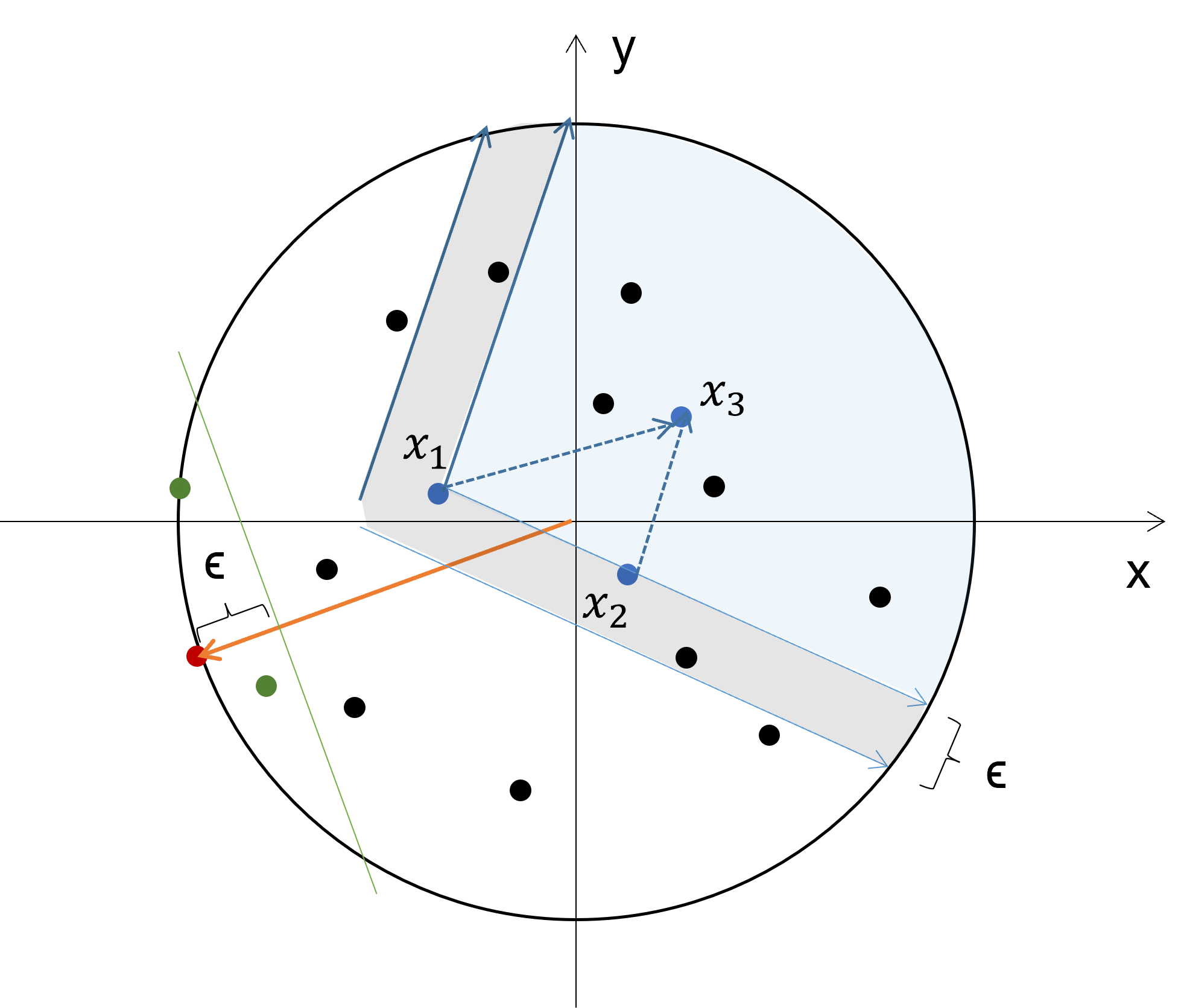
Figure 1. An illustrative example for a filter in Algorithm 2. The unknown utility vector $\mathbf{u}$ is drawn in orange. Every tuple is shown as a point within a unit circle, where the red point represents the top tuple, and green points are feasible $\epsilon$-regret tuples for the $\mathrm{IRM}$ problem. Suppose a filter collects a random sample $S$ of blue points. A sorted sample $S$ can be used to prune any point that falls into or is sufficiently close to (within a distance of $\epsilon$) the blue cone.

An example that illustrates the mechanism of a filter is displayed in Fig. 1, on which we elaborate below.

Example 0.

In Fig. 1, a random sample $S=\{\mathbf{x}_{1},\mathbf{x}_{2},\mathbf{x}_{3}\}$ of three blue points is collected and sorted, where $\mathbf{x}_{1}$ has the highest utility. This means that $\text{util}(\mathbf{x}_{j+1})-\text{util}(\mathbf{x}_{j})=\mathbf{u}^{T}(\mathbf{x}_{j+1}-\mathbf{x}_{j})<0$, for any $j\in\{1,2\}$. Compared to the point $\mathbf{x}_{1}$, a new point $\mathbf{x}$ in the form of $\mathbf{x}=\mathbf{x}_{1}+\sum_{j\in\{1,2\}}\alpha_{j}(\mathbf{x}_{j+1}-\mathbf{x}_{j})$ with $\alpha_{j}\geq 0$ can only have a lower utility than $\text{util}(\mathbf{x}_{1})$, since

$$\text{util}(\mathbf{x})=\mathbf{u}^{T}\bigg{[}\mathbf{x}_{1}+\sum_{j\in\{1,2\}}\alpha_{j}(\mathbf{x}_{j+1}-\mathbf{x}_{j})\bigg{]}\leq\text{util}(\mathbf{x}_{1}).$$

Thus, such a point $\mathbf{x}$ can be safely pruned. Geometrically, all such prunable points $\mathbf{x}$ form a cone with apex $\mathbf{x}_{1}$, as highlighted in the blue region in Fig. 1. According to Eq. 2, any point that is sufficiently close to (within a distance of $\epsilon$) the blue cone can also be pruned.

Upon a random-order stream of tuples, Algorithms 1 and 2 collect a pool $P$ of $p$ initial tuples as a testbed for filter performance. Then, subsequent tuples are gradually added into the first sample set $S_{1}$, until a filter based on $S_{1}$ can prune at least a $\theta=5/8$ fraction of $P$. Then, $S_{1}$ is ready, and is used to prune tuples in the pool $P$ and future tuples over the stream. Future tuples that survive the filter formed by $S_{1}$ will be gradually added into the pool $P$ and a second sample set $S_{2}$, and the process is repeated iteratively. Finally, the algorithm returns the best tuple among all samples. The following theorem states our main result about Algorithms 1 and 2.

Theorem 2.

Assume $\epsilon>0$ and let $n=|D|$ be the size of data. Let $c=\text{util}(\mathbf{x}^{*})\in[0,1]$ be the utility of the best tuple $\mathbf{x}^{*}$. Under 1, with a pool size $p=\left\lceil{64\ln 2n}\right\rceil$ and $\theta=5/8$, Algorithms 1 and 2 return an $\epsilon/c$-regret tuple for the $\mathrm{IRM}$ problem.

Let $t=16d\ln(2d/\epsilon)$, where $d$ is the intrinsic dimension of $D$. Then, with probability at least $1-1/n$, at most

$$\mathcal{O}(\log(n)\,4t\log(4t))+p$$

comparisons are made.

The memory size, i.e., the number of tuples that will be kept by the algorithm during the execution, is $\mathcal{O}(\log(n)\,4t)$, which is also logarithmic in $n$.

In fact, Algorithms 1 and 2 are an anytime algorithm, in the sense that the data stream can be stopped anytime, while the algorithm is still able to return a feasible solution among all tuples that have arrived so far.

Theorem 3.

Under 1, the data stream may terminate at any moment during the execution of Algorithms 1 and 2, and an $\epsilon/c$-regret tuple will be returned for the $\mathrm{IRM}$ problem among all tuples that have arrived so far.

Proofs of Theorems 2 and 3 are deferred to Appendix A.

5. Finding a tuple: oracle with ties

In this section, we first introduce a natural notion of uncomparable pairs to avoid error-prone comparisons, and then we show how this new setting affects our algorithms.

It is clearly more difficult for a user to distinguish a pair of tuples with nearly equal utility. Thus, it is reasonable to not force the user to make a choice in the face of a close pair, and allow the user to simply declare the comparison a tie instead. We make this intuition formal below.

Definition 0 ($\mathbf{u}$-similar pairs).

Two tuples $\mathbf{x},\mathbf{y}\in D$ are $\mathbf{u}$-similar if

$$|\text{util}(\mathbf{x})-\text{util}(\mathbf{y})|\leq\tau,$$

for some fixed value $\tau$. We write $\mathbf{x}\sim\mathbf{y}$ if they are uncomparable.

Assumption 2.

A query about a $\mathbf{u}$-similar pair to the oracle will be answered with a tie. Besides, as before, we assume that the best tuple $\mathbf{x}^{*}$ has non-negative utility, $\text{util}(\mathbf{x}^{*})\geq 0$.

Typically, the value $\tau$ is fixed by nature, unknown to us, and cannot be controlled. Note that when $\tau$ is sufficiently small, we recover the previous case in Section 4 where every pair is comparable under 1. By allowing the user to not make a clear-cut comparison for a $\mathbf{u}$-similar pair, one can no longer be guaranteed total sorting. Indeed, it could be that every pair in $D$ is $\mathbf{u}$-similar.

In Algorithm 3, we provide a filter to handle ties under 2. We maintain a totally sorted subset $R$ of representative tuples in a sample set $S$. For each representative $\mathbf{y}\in R$, we create a group $G_{\mathbf{y}}$. Upon the arrival of a new tuple $\mathbf{x}$, we sort $\mathbf{x}$ into $R$ if no tie is encountered. Otherwise, we encounter a tie with a tuple $\mathbf{y}\in R$ such that $\mathbf{x}\sim\mathbf{y}$, and we add $\mathbf{x}$ into a group $G_{\mathbf{y}}$. In the end, the best tuple in $R$ will be returned.

Input: parameter $\epsilon$

1 Class NewFilter:  $R\leftarrow\emptyset,\,S\leftarrow\emptyset$;

2

3Function prune$(\mathbf{x})$:

4       return true, if $S\overset{\text{sim}}{\Rightarrow}\mathbf{x}$ (see Eq. 5), otherwise false

5      

6

7Function add$(\mathbf{x})$:

8       $S\leftarrow S\cup\{\mathbf{x}\}$, and sort $\mathbf{x}$ within $R$

9       if no tie happens then

10             $R\leftarrow R\cup\{\mathbf{x}\}$ and create $G_{\mathbf{x}}\leftarrow\{\mathbf{x}\}$

11            

12      else

13             Encounter a tie with $\mathbf{y}\in R$ such that $\mathbf{x}\sim\mathbf{y}$

14             $G_{\mathbf{y}}\leftarrow G_{\mathbf{y}}\cup\{\mathbf{x}\}$

15            

16      

17

18Function best$()$:  return the best tuple in $R$

19

Algorithm 3 Functions that define a filter for the $\mathrm{IRM}$ problem with ties

To see whether a filter in Algorithm 3 can prune a given tuple $\mathbf{x}$, we test the following condition. Let $R=\mathbf{x}_{1},\ldots$ be the sorted list of representive tuples, where $\mathbf{x}_{1}$ is the top tuple. Let $\mathcal{G}=G_{1},\ldots$ be the corresponding groups. A tuple $\mathbf{x}$ can be pruned if there exists $\mathbf{x}^{\prime}$ such that $\left\lVert\mathbf{x}-\mathbf{x}^{\prime}\right\rVert_{2}\leq\epsilon$, where

(4) $$\mathbf{x}^{\prime}= \sum_{\mathbf{y}\in G_{1}\cup G_{2}}\nu_{\mathbf{y}}\,\mathbf{y}+\sum_{j=1}\sum_{\mathbf{z}\in G_{j}}\sum_{\mathbf{w}\in G_{{j+2}}}\alpha_{\mathbf{w},\mathbf{z}}(\mathbf{w}-\mathbf{z})$$

$$\text{such that}\sum_{\mathbf{y}\in G_{1}\cup G_{2}}\nu_{\mathbf{y}}=1\text{ and all }\nu,\alpha\geq 0.$$

The idea is similar to Eq. 2, except that the top tuple $\mathbf{x}_{1}$ in Eq. 2 is replaced by an aggregated tuple by convex combination, and every pair difference $\mathbf{x}_{j+1}-\mathbf{x}_{j}$ is replaced by pair differences between two groups. We avoid using pair differences between two consecutive groups, as tuples in group $G_{j}$ may not have higher utility than tuples in $G_{{j+1}}$. If the above condition is met, then we write

(5) $$\mathcal{G}\overset{\text{sim}}{\Rightarrow}\mathbf{x}\quad\text{and, if $\mathcal{G}$ is constructed using $S$,}\quad S\overset{\text{sim}}{\Rightarrow}\mathbf{x}.$$

The number of comparisons that is needed by Algorithm 3 depends on the actual input, specifically, $\xi$, the largest size of any pairwise $\mathbf{u}$-similar subset of $D$. Note that the guarantee below recovers that of Theorem 2 up to a constant factor, if assuming 1 where $\xi=1$. However, in the worst case, $\xi=\mathcal{O}(n)$ and the guarantee becomes vacuous.

Theorem 2.

Assume $\epsilon>0$ and let $n=|D|$ be the size of data. Let $c=\text{util}(\mathbf{x}^{*})\in[0,1]$ be the utility of the best tuple $\mathbf{x}^{*}$. Under 2, with a pool size $p=\left\lceil{256\ln 2n}\right\rceil$ and $\theta=3/16$, Algorithms 1 and 3 return an $(\epsilon/c+2\tau)$-regret tuple for the $\mathrm{IRM}$ problem.

Let $t=16d\ln(2d/\epsilon)$, where $d$ is the intrinsic dimension of $D$, and $\xi$ be the largest size of a pairwise $\mathbf{u}$-similar subset of $D$. Then, with probability at least $1-1/n$, at most

$$\mathcal{O}(\log(n)\,16t\xi\log(16t\xi))+p$$

comparisons are made.

Proofs of Theorem 2 are deferred to Appendix B.

6. Improving baseline filters

In this section, we improve existing filters by xie2019strongly, by using linear and quadratic programs. We will use these baselines in the experiments. Previously, their filters rely on explicit computation of convex hulls, which is feasible only in very low dimension (barber1996quickhull). Technical details are deferred to Appendix C.

Existing filters iteratively compare a pair of random tuples, all of which are kept in $A=\{a_{i}\}$, where $a_{i}=(\mathbf{y},\mathbf{z})$ such that $\text{util}(\mathbf{y})<\text{util}(\mathbf{z})$, and use them to prune potential tuples.

Filter by constrained utility space

Given a tuple $\mathbf{x}$, we try to find a vector $\mathbf{u}$ that, for all $(\mathbf{y},\mathbf{z})\in A$,

(6) $$\mathbf{u}^{T}(\mathbf{z}-\mathbf{y})\geq 1,\quad\mathbf{u}^{T}(\mathbf{x}-\mathbf{z})\geq 1,\quad\mathbf{u}^{T}((1-\epsilon)\mathbf{x}-\mathbf{z})\geq 1.$$

We claim that a given tuple $\mathbf{x}$ can be safely pruned if there is no vector $\mathbf{u}$ satisfying LP (Eq. 6).

Proposition 1.

Consider a tuple $\mathbf{x}$ with $\text{util}(\mathbf{x})>\text{util}(\mathbf{z})$ and $\text{util}(\mathbf{x})-\text{util}(\mathbf{z})>\epsilon\text{util}(\mathbf{x})$ for every $(\mathbf{y},\mathbf{z})\in A$. Then there is a solution to LP (Eq. 6).

Filter by conical hull of pairs

Given a tuple $\mathbf{x}$, we propose to solve the following quadratic program (QP),

(7) $$\min_{\nu,\beta}\bigg{\|}\mathbf{x}-\sum_{a_{i}=(\mathbf{y},\mathbf{z})\in A}(\nu_{i1}\,\mathbf{y}+\nu_{i2}\,\mathbf{z})-\sum_{a_{i}=(\mathbf{y},\mathbf{z})\in A}\beta_{i}(\mathbf{y}-\mathbf{z})\bigg{\|}$$

$$\text{such that}\sum_{a_{i}=(\mathbf{y},\mathbf{z})\in A}\nu_{i1}+\nu_{i2}=1\quad\text{and}\quad\nu_{i1},\nu_{i2},\beta_{i}\geq 0\quad\text{for all }i.$$

If the optimal value of the QP is at most $\epsilon$, we prune $\mathbf{x}$.

Proposition 2.

Let $\mathbf{u}^{T}\mathbf{x}^{*}=c$. A tuple $\mathbf{x}\in D$ can be pruned if the objective value of the quadratic program (Eq. 7) is at most $\epsilon/c$.

If we set $\epsilon=0$, then we can use LP solver (similar to Eq. 1) instead of QP solver. This results in a weaker but computationally more efficient filter.

7. Experimental evaluation

In this section, we evaluate key aspects of our method and the proposed filters. Less important experiments and additional details are deferred to Appendix D. In particular, we investigate the following questions. ($i$) How accurate is the theoretical bound in Lemma 3? More specifically, we want to quantify the sample size required by Algorithm 2 to prune at least half of the tuples, and understand its dependance on the data size $n$, dimension $d$, and regret parameter $\epsilon$. ($ii$) Effect of parameters of Algorithm 1. (Section D.1) ($iii$) How scalable are the proposed filters? ($iv$) How do the proposed filters perform over real-life datasets? ($v$) How do ties in comparisons affect the performance of the proposed filters? Our implementation is available at a Github repository.

Next, let us introduce the adopted datasets and baselines.

Datasets. A summary of the real-life datasets we use for our evaluation can be found in Table 2. To have more flexible control over the data parameters, we additionally generate the following two types of synthesized data. sphere: Points sampled from the unit $d$-sphere $\mathbb{S}^{d-1}$ uniformly at random. clusters: Normally distributed clustered data, where each cluster is centered at a random point on unit $d$-sphere $\mathbb{S}^{d-1}$. To simulate an oracle, we generate a random utility vector $\mathbf{u}$ on the unit $d$-sphere for every run. More details about datasets can be found in Appendix D.

Baselines. A summary of all algorithms is given in Table 3. We mainly compare with (enhanced) pruning techniques (Pair-QP, Pair-LP and HS-LP) by xie2019strongly, halfspace-based pruning (HS), and a random baseline (Rand). Discussion of other baselines is deferred to Appendix D. We instantiate every filter (except for the HS and Rand) in the framework provided in Algorithm 1, that is, we iteratively create a new filter that can prune about half of the remaining tuples. This is a reasonable strategy, and will be justified in detail in Section 7.2. For pair-based filters, a new pair is made after two consecutive calls of the add function. The pool size $p$ and threshold $\theta$ in Algorithm 1 are set to be 100 and 0.5, respectively. Since the proposed algorithm List-QP only guarantees a regret of $\epsilon/\text{util}(x^{*})$, where $x^{*}$ is the best tuple in the dataset, we pre-compute the value of $\text{util}(x^{*})\in[0,1]$, and adjust the regret parameter of List-QP to be $\epsilon\text{util}(x^{*})$.

Table 2. Real-life datasets statistics

Dataset	$n=|D|$	$d$
player (dataplayer)	17 386	20
youtube (datayoutube)	29 406	50
game (datagame)	60 496	100
house (datahouse)	303 032	78
car (datacar)	1 002 350	21

Table 3. Summary of our methods and the baselines.

Name	Brief description
List-[QP|LP]	Our method: prune a tuple if it is close to a conical hull formed by a sorted list of random tuples (Algorithm 2), equipped with a QP or LP solver.
Pair-[QP|LP]	Prune a tuple if it is close to a conical hull formed by a set of compared random pairs, equipped with QP (Eq. 7) or LP solver.
HS-LP	Prune a tuple if LP (Eq. 6) is infeasible, i.e., the tuple is dominated by a set of compared random pairs over the entire constrained utility space.
HS	Prune a tuple $\mathbf{x}$ if $\mathbf{x}^{T}(\mathbf{z}-\mathbf{y})<0$ for any compared pair $\mathbf{z},\mathbf{y}$ such that $\text{util}(\mathbf{y})<\text{util}(\mathbf{z})$, that is, tuple $\mathbf{x}$ falls outside the constrained utility space for $\mathbf{u}$.
Rand	Return the best tuple among a subset of 50 random tuples.

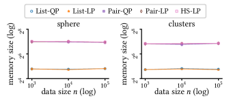
(a) Memory size required to prune half of tuples

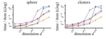
(b) Scalability with respect to dimension $d$

Figure 2. Scalability of filters for synthetic data

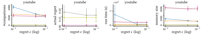
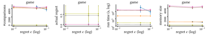
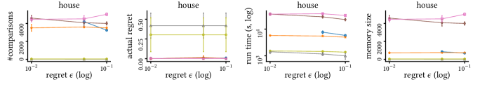
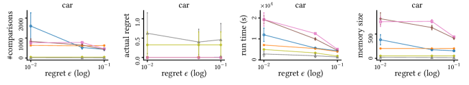
Figure 3. Solving the $\mathrm{IRM}$ problem on the real-life datasets

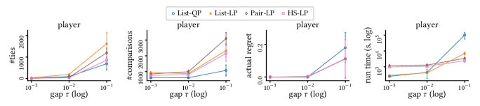
Figure 4. The effect of ties and parameter $\tau$

7.1. Sample size in practice

Lemma 3 proves a theoretical bound on the size of a random sample required by Algorithm 2 to prune at least half of a given set $D$ of tuples in expectation. This bound is $2t$ where $t=16d\ln(2d/\epsilon)$. Importantly, the bound does not depend on the data size $|D|$, which we verify later in Section 7.2.

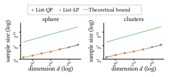
(a)

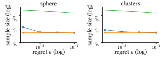
(b)

Figure 5. Sample size required to prune half of tuples, as a function of the data dimension (a), and as a function of the regret parameter (b)

In Figs. 5(a) and 5(b) (in Appendix), we compute and present the exact required size for synthesized data, and illustrate how the size changes with respect to the dimension $d$ and regret parameter $\epsilon$. As can be seen, the bound provided in Lemma 3 captures a reasonably accurate dependence on $d$ and $\epsilon$, up to a constant factor.

7.2. Scalability

The running time required for each filter to prune a given tuple depends heavily on its memory size, i.e., the number of tuples it keeps. In Fig. 2(a), we compute and show the required memory size for a filter to prune half of a given set $D$ of tuples, and how the size changes with respect to the data size $n=|D|$. Impressively, most competing filters that adopt a randomized approach only require constant memory size, regardless of the data size $n$. This also confirms the effectiveness of randomized algorithms in pruning.

Based on the above observation, it is usually not feasible to maintain a single filter to process a large dataset $D$. If a filter requires $s$ tuples in memory to prune half of $D$, then at least $s\log(|D|)$ tuples are expected to process the whole dataset $D$. However, the running time for both LP and QP solvers is superlinear in the memory size of a filter (cohen2021solving), which means that running a filter with $s\log(|D|)$ tuples is considerably slower than running $\log(|D|)$ filters, each with $s$ tuples. The latter approach enables also parallel computing for faster processing.

Therefore, we instantiate each competing filter (except for HS and Rand) in the framework provided in Algorithm 1, and measure the running time it takes to solve the $\mathrm{IRM}$ problem. In the rest of this section, we investigate the effect of the data dimension $d$ and regret parameter $\epsilon$ on the running time.

Effect of data dimension $d$. In Fig. 2(b), we fix a regret parameter $\epsilon=0.01$, and examine how the running time of a filter varies with respect to the data dimension $d$ on synthesized data.

The first observation from Fig. 2(b) is that LP-based filters are more efficient than their QP counterparts. Particularly, Pair-QP is too slow to be used, and we have to settle for its LP counterpart Pair-LP in subsequent experiments.

Let us limit the comparison to those LP-based filters. Pair-LP and HS-LP are more computationally expensive than List-LP. For Pair-LP, the reason is obvious: as discussed at the end of Section C.2, Pair-LP makes relatively more comparisons and every compared pair of tuples adds two more parameters to the LP. For HS-LP, the number of parameters in its LP depends linearly on both the dimension $d$ and number of compared pairs, while List-LP only depends on the latter. Thus, HS-LP is less scalable by design.

Effect of regret parameter $\epsilon$. The effect of the regret parameter $\epsilon$ can be found in Fig. 3 for all real-life datasets. Generally, a larger value of $\epsilon$ decreases the running time, as each filter can be benefited by more aggressive pruning.

The running time of List-QP deteriorates dramatically for a small value of $\epsilon$, and the number of comparisons needed also rises considerably. The reason is that, most numerical methods for solving a mathematical program have a user-defined precision parameter. Small precision gives a more accurate solution, and at the same time causes a longer running time. When $\epsilon$ gets close to the default precision, or to the actual precision after the maximum number of iterations is exceeded, List-QP fails to prune tuples. Thus, List-QP is advised to be used for a relatively large regret value $\epsilon$.

In regard to the memory size, as we can see in Fig. 3, List-QP and List-LP consistently use a much smaller memory size than Pair-LP and HS-LP. This also demonstrates the advantage of using a sorted list over a set of compared pairs.

7.3. The case of oracles with no ties

The performance of competing filters can be found in Fig. 3 for all real-life datasets. The average and standard error of three random runs are reported. We instantiate each competing filter (except for HS and Rand) in the framework provided in Algorithm 1 to solve the $\mathrm{IRM}$ problem. Meanwhile, we vary the regret parameter $\epsilon$ to analyze its effect. We also experimented with a smaller $\epsilon$ value such as 0.005, the observations are similar except that the List-QP filter is significantly slower for reasons we mentioned in Section 7.2.

Except HS and Rand, every reasonable filter succeeds in returning a low-regret tuple. We limit our discussion to only these reasonable filters. In terms of the number of comparisons needed, List-QP outperforms the rest on most datasets provided that the regret value $\epsilon$ is not too small. We rate List-LP as the runner-up, and it becomes the top one when the regret value $\epsilon$ is small. Besides, List-LP is the fastest to run. The number of comparisons needed by HS-LP and Pair-LP is similar, and they sometimes perform better than others, for example, over the youtube dataset.

Let us make a remark about the regret value $\epsilon$. Being able to exploit a large value of $\epsilon$ in pruning is the key to improving performance. Notice that both Pair-LP and List-LP cannot benefit from a large regret value $\epsilon$ by design. Though HS-LP is designed with $\epsilon$ in mind, it is more conservative as its pruning power depends on $\epsilon\mathbf{u}^{T}\mathbf{x}$ instead of $\epsilon\mathbf{u}^{T}\mathbf{x}^{*}$, where $\mathbf{x}$ is the tuple to prune.

In summary, we can conclude that the List-QP filter is recommended for a not too small regret parameter $\epsilon$ (i.e., $\epsilon\geq 0.1$), and the List-LP filter is recommended otherwise. In practice, since both List-QP and List-LP follow an almost identical procedure, one could always start with List-QP, and switch to List-LP if the pruning takes too long time.

7.4. Effect of ties

According to 2, the oracle returns a tie if the difference in utility between two given tuples is within a parameter $\tau$. For filters like Pair-LP and HS-LP, the most natural strategy to handle a tie for a pair of tuples is to simply discard one of them. It is expected that ties worsen the performance of a filter, as they fail to provide additional information required by the method for pruning.

In Fig. 4, we vary the value of parameter $\tau$ to see how it affects the performance of the proposed filters. It is not surprising that as the value of $\tau$ increases, the number of ties encountered and the number of comparisons made by all algorithms both increase.

Notably, the running time of List-QP and List-LP grows significantly as $\tau$ increases. This is because one parameter is needed in their solvers for every pair of tuples between two consecutive groups $G_{i},G_{j}$, and the total number of parameters can increase significantly if the size of both groups increases. This behavior also reflects the fact that a partially sorted list is less effective for pruning. However, how to handle a large $\tau$ remains a major open problem. Hence, we conclude that the proposed algorithms work well provided that the parameter $\tau$ is not too large.

Summary

After the systematical evaluation, we conclude with the following results. ($i$) LP-based filters are more efficient than their QP counterparts, but less effective in pruning. ($ii$) List-LP is the most scalable filter. The runner-up is List-QP, provided that the data dimension is not too large ($d<128$) and the regret parameter $\epsilon$ is not too small ($\epsilon\geq 0.1$). ($iii$) To minimize the number of requested comparisons, List-QP is recommended for a not too small $\epsilon$ ($\epsilon\geq 0.1$). When $\epsilon$ is small, we recommend List-LP. ($iv$) Good performance can be retained if the oracle is sufficiently discerning ($\tau\leq 0.01$). Otherwise, a better way to handle ties will be needed.

8. Conclusion

We devise a single-pass streaming algorithm for finding a high-utility tuple by making adaptive pairwise comparisons. We also show how to maintain the guarantee when ties are allowed in a comparison between two tuples with nearly equal utility. Our work suggests several future directions to be explored. Those include finding a high-utility tuple in the presence of noise, incorporating more general functions for modeling tuple utility, devising methods with provable quarantees for arbitrary-order data streams, and devising more efficient algorithms to handle ties.

Appendix A Proofs for Section 4

kane2018generalized proved a powerful local lemma, which states that among a sufficiently large set of vectors from the unit $d$-ball $\mathcal{B}^{d}$, there must exist some vector that can be approximately represented as a special non-negative linear combination of others.

Lemma 1 ((kane2018generalized), Claim 15).

Given $\mathbf{x}_{1},\ldots,\mathbf{x}_{t}\in\mathcal{B}^{d}$, for any $\epsilon>0$, if $t\geq 16d\ln(2d/\epsilon)$, then there exists $a\in[t]$ such that

(8) $$\mathbf{x}_{a}=\mathbf{x}_{1}+\sum_{j=1}^{a-2}\alpha_{j}(\mathbf{x}_{j+1}-\mathbf{x}_{j})+\mathbf{e},$$

where $\left\lVert\mathbf{e}\right\rVert_{2}\leq\epsilon$ and $\alpha_{j}\in\{0,1,2\}$.

Let $S=\{\mathbf{x}_{1},\ldots,\mathbf{x}_{t}\}$. Lemma 1 can be easily extended to hold for the intrinsic dimension of $S$, by first applying Lemma 1 to the minimal representation $\mathbf{y}_{1},\ldots,\mathbf{y}_{t}\in\mathcal{B}^{d^{\prime}}$ of $S$.

In Lemma 1, we have $S-\mathbf{x}_{a}\Rightarrow\mathbf{x}_{a}$, where $S-\mathbf{x}$ is a shorthand for $S\setminus\{\mathbf{x}\}$. Note that this is exactly the condition we use in Step 2 in Algorithm 2 for pruning. Denote by $\text{filter}(S)$ the set of all such pruned tuples, i.e.,

(9) $$\text{filter}(S)=\{\mathbf{x}\in\mathbb{R}^{d}:S\Rightarrow\mathbf{x}\}.$$

Given any set $S$ of size $4t$, at least 3/4 fraction of $S$ can be pruned by other tuples in $S$, by repeatedly applying Lemma 1.

Lemma 2.

Given a sorted set $S$ of size at least $4t$, where $t=16d\ln(2d/\epsilon)$, we have

$$|\{\mathbf{x}\in S:S-\mathbf{x}\Rightarrow\mathbf{x}\}|\geq\frac{3}{4}|S|.$$

Proof.

since $|S|\geq 4t$, we can apply Lemma 1 repeatedly to $S$ until only $t$ entries remain. ∎

As a consequence of Lemma 2, the same fraction of current tuples $X$ can be pruned by a random sample set $S$ of a sufficient size in expectation.

Lemma 3.

Given a set of tuples $X$, and a random sample set $S\subseteq X$ of size $4t$ where $t=\left\lceil{16d\ln(2d/\epsilon)}\right\rceil$, we have

$$\mathsf{E}\left[|\text{filter}(S)\cap X|\right]\geq\frac{3}{4}|X|,$$

where the expectation is taken over $S$.

Another important issue to handle is to ensure that our pruning strategy will not discard all feasible tuples. This is prevented by keeping track of the best tuple in any sample set so far, and guaranteed by Theorem 3.

Proof of Theorem 3.

Denote by $D$ all tuples that have arrived so far. Suppose $\mathbf{x}^{*}$ is the best tuple among $D$. Tuple $\mathbf{x}^{*}$ is either collected into our sample sets, or pruned by some sample set $S$. In the former case, our statement is trivially true. In the latter case, suppose $S=\{\mathbf{x}_{1},\ldots\}$, where $\mathbf{x}_{1}$ is the best tuple in $S$. If $\mathbf{x}_{1}$ is feasible, then $\hat{\mathbf{x}}$ is feasible as well, as it is at least as good as $\mathbf{x}_{1}$. If $\mathbf{x}_{1}$ is infeasible, i.e., $\text{util}(\mathbf{x}^{*})-\text{util}(\mathbf{x}_{1})>\epsilon$, then $\mathbf{x}^{*}$ cannot be pruned by $S$ by design, a contradiction. This completes the proof. ∎

Before proving Theorem 2, we briefly summarize the hypergeometric tail inequality below (skala2013hypergeometric).

Lemma 4 (Hypergeometric tail inequality (skala2013hypergeometric)).

Draw $n$ random balls without replacement from a universe of $N$ red and blue balls, and let $i$ be a random variable of the number of red balls that are drawn. Then, for any $t>0$, we have

$$\Pr[i\geq\mathsf{E}[i]+tn]\leq e^{-2t^{2}n},$$

and

$$\Pr[i\leq\mathsf{E}[i]-tn]\leq e^{-2t^{2}n}.$$

Proof of Theorem 2.

The feasibility of the returned tuple $\hat{\mathbf{x}}$ is due to Theorem 3. In the rest of the proof, we upper bound the size of every sample and the number of samples we keep in the sequence $\mathcal{S}$.

For any sample $S$ with at least $4t$ samples and any subset $X\subseteq D$, let $X^{\prime}=\text{filter}(S)\cap X$ and by Lemma 3 we have $\mathsf{E}[|X^{\prime}|]\geq\frac{3}{4}|X|$. In particular, let $X=P$ and we have $\mathsf{E}[|P^{\prime}|]\geq\frac{3}{4}|P|$ and $|P|=p$. Then,

$$\Pr\left[|P^{\prime}|<\frac{5}{8}|P|\right] =\Pr\left[|P^{\prime}|<\frac{3}{4}|P|-\frac{1}{8}p\right]$$

$$\leq\Pr\left[|P^{\prime}|<\mathsf{E}[|P^{\prime}|-\frac{1}{8}p]\right]\leq e^{-2p/8^{2}},$$

where the last step invokes Lemma 4. Since there can be at most $n$ samples, the probability that any sample fails to pass the pool test is upper bounded by $ne^{-2p/8^{2}}$.

We continue to upper bound the number of sample sets. At most $\left\lceil{\log(n)}\right\rceil$ sample sets suffice if every sample can prune at least half of the remaining tuples. Fix an arbitrary sample $S$, and let $X$ to be the set of remaining tuples. The pool $P$ is a random sample from $X$ of size $p$. Thus, $\mathsf{E}[|P^{\prime}|]/p=|X^{\prime}|/|X|$. Consequently, if $|X^{\prime}|<|X|/2$, then $\mathsf{E}[|P^{\prime}|]<p/2$ and

$$\Pr\left[|P^{\prime}|\geq\frac{5}{8}|P|\right]\leq\Pr\left[|P^{\prime}|\geq\mathsf{E}[|P^{\prime}|]+\frac{1}{8}p\right]\leq e^{-2p/8^{2}}.$$

Similar to the above, the probability that any bad sample passes the test is upper bounded by $ne^{-2p/8^{2}}$.

Combining the two cases above, the total failure probability is $2ne^{-2p/8^{2}}\leq 1/n$ Hence, with probability at least $1-1/n$, it is sufficient to use $\left\lceil{\log(n)}\right\rceil$ sample sets, each with a size $4t$. Keeping one sample set requires $4t\left\lceil{\log(4t)}\right\rceil$ comparisons. Finally, finding the best tuple among all filters and the pool requires additional $p+\left\lceil{\log(n)}\right\rceil$ comparisons. ∎

Appendix B Proofs for Section 5

The proof is similar to that of Theorem 2, except that we need a new proof for the key Lemma 3, since in the presence of ties, we may not be able to totally sort a sample $S$. Instead, we show that a partially sorted set $S$ of a sufficient size can also be effective in pruning.

From now on, we treat the sample $S$ as a sequence instead of a set, as a different arrival order of $S$ may result in a different filter by Algorithm 3.

Lemma 1.

Let $S\subseteq X$ be a sequence of length $16t\xi$. Let $\mathcal{G}$ be the groups constructed by Algorithm 3. Under 2, we have

$$|\{\mathbf{x}\in S:\mathcal{G}-\mathbf{x}\overset{\text{sim}}{\Rightarrow}\mathbf{x}\}|\geq\frac{3}{4}|S|,$$

where $t=16d\ln(2d/\epsilon)$, $\xi$ is the largest size of a pairwise $\mathbf{u}$-similar subset of $X$, and $\mathcal{G}-\mathbf{x}$ are the groups with $\mathbf{x}$ removed from its group.

Although the above lemma appears similar to Lemma 2, a crucial difference is that the set of prunable tuples in $S$ now depends on the arrival order of $S$, which causes non-trivial technical challenges in the analysis. A critical observation that enables our analysis is the following result.

Lemma 2.

Fix a sequence $S$ of size $16t\xi$, there exist at least $\frac{1}{4}|S|$ tuples $\mathbf{z}$ in $S$ that satisfy

$$S-\mathbf{z}\overset{\text{sim}}{\Rightarrow}\mathbf{z}.$$

Denote by $\text{filter-sim}(S)$ the set of tuples that can be pruned by $S$, that is,

(10) $$\text{filter-sim}(S)=\{\mathbf{x}\in\mathbb{R}^{d}:S\overset{\text{sim}}{\Rightarrow}\mathbf{x}\}.$$

We now prove a similar lemma to Lemma 3 by a generalized symmetrization argument over sequences.

Lemma 3.

Given a set of tuples $X$, and a random sequence $S$ of at least $16t\xi$ tuples from $X$, we have

$$\mathsf{E}\left[|\text{filter-sim}(S)\cap X|\right]\geq\frac{1}{4}|X|,$$

where $t=16d\ln(2d/\epsilon)$, and $\xi$ is the largest size of a pairwise $\mathbf{u}$-similar subset of $X$. Moreover, the expectation is taken over $S$.

Appendix C Improving baseline filters

In this section, we improve existing filters by xie2019strongly, by using linear and quadratic programs. Previously, their filters rely on explicit computation of convex hulls, which is feasible only in very low dimension. For example, the convex hull size, and consequently the running time of these existing techniques, have an exponential dependence on $d$ (barber1996quickhull).

C.1. Improving constrained utility space filter

One of the most natural strategies is to iteratively compare a pair of random tuples. The feasible space for the utility vector $\mathbf{u}$ is constrained by the list of pairs $A=\{a_{i}\}$ that have been compared, where $a_{i}=(\mathbf{y},\mathbf{z})$ such that $\text{util}(\mathbf{y})<\text{util}(\mathbf{z})$. Note that every pair of tuples $\mathbf{y},\mathbf{z}\in D$ forms a halfspace in $\mathbb{R}^{d}$, i.e., $H=\{\mathbf{u}\in\mathbb{R}^{d}:\mathbf{u}^{T}(\mathbf{y}-\mathbf{z})<0\}$. Specifically, the unknown $\mathbf{u}\in\mathbb{S}^{d-1}$ is contained in the intersection $U$ of a set of halfspaces, one by each pair.

xie2019strongly propose to prune a tuple $\mathbf{x}$ if for every possible $\mathbf{u}\in U$ there exists a tuple $\mathbf{w}$ in some pair of $A$ such that $\text{util}(\mathbf{w})\geq\text{util}(\mathbf{x})$. They first compute all extreme points of $U$, and then check if the condition holds for every extreme point. However, this approach is highly inefficient, as potentially there is an exponential number of extreme points.

Instead, we propose to test the pruning condition by asking to find a vector $\mathbf{u}$ that satisfies

(6) $$\mathbf{u}^{T}(\mathbf{z}-\mathbf{y})\geq 1,\quad\mathbf{u}^{T}(\mathbf{x}-\mathbf{z})\geq 1,\quad\mathbf{u}^{T}((1-\epsilon)\mathbf{x}-\mathbf{z})\geq 1.$$

If there is no such vector $\mathbf{u}$ we prune $\mathbf{x}$. This test can be done with a linear program (LP). Note that the test is stronger than that by xie2019strongly as it has been extended to handle $\epsilon$-regret.

We claim that a given tuple $\mathbf{x}$ can be safely pruned if there is no vector $\mathbf{u}$ satisfying LP (Eq. 6).

See 1

Notice that the second set of constraints in LP (Eq. 6) (i.e., $\mathbf{u}^{T}(\mathbf{x}-\mathbf{z})\geq 1$) is redundant provided $\text{util}(\mathbf{x})\geq 0$. Actually, even if $\text{util}(\mathbf{x})<0$, the test only lets in $\mathbf{x}$ that is slightly worse than the best tuple in $A$, which is unlikely since $\text{util}(\mathbf{x})<0$. Thus, in practice we recommend to omit the second set of constraints to speed up the test.

A filter for maintaining the constrained utility space is conceptually different from the filter proposed in Section 4. A small utility space of $\mathbf{u}$ is the key for such a filter to be effective, while a filter in Section 4 maintains no explicit knowledge about $\mathbf{u}$ and mainly relies on the geometry of the tuples.

C.2. Improving conical hull of pairs filter

Another pruning strategy proposed by xie2019strongly is the following. Consider again a list of compared pairs $A=\{a_{i}\}$, where $a_{i}=(\mathbf{y},\mathbf{z})$ such that $\text{util}(\mathbf{y})<\text{util}(\mathbf{z})$, and consider a cone formed by all pairs in $A$. A tuple $\mathbf{x}$ can now be pruned if there is another tuple $\mathbf{w}$ kept by the algorithm, such that

$$\mathbf{x}=\mathbf{w}+\sum_{a_{i}=(\mathbf{y},\mathbf{z})\in A}\beta_{i}(\mathbf{y}-\mathbf{z})\quad\text{such that}\quad\beta_{i}\geq 0\quad\text{for all }i.$$

Instead of actually constructing all facets of the conical hull, as done by xie2019strongly, we propose to solve the following quadratic program (QP),

$$\min_{\nu,\beta}\bigg{\|}\mathbf{x}-\sum_{a_{i}=(\mathbf{y},\mathbf{z})\in A}(\nu_{i1}\,\mathbf{y}+\nu_{i2}\,\mathbf{z})-\sum_{a_{i}=(\mathbf{y},\mathbf{z})\in A}\beta_{i}(\mathbf{y}-\mathbf{z})\bigg{\|}$$

(7) $$\text{such that}\sum_{a_{i}=(\mathbf{y},\mathbf{z})\in A}\nu_{i1}+\nu_{i2}=1\quad\text{and}\quad\nu_{i1},\nu_{i2},\beta_{i}\geq 0\quad\text{for all }i.$$

If the optimal value of the QP is at most $\epsilon$, we prune $\mathbf{x}$.

See 2

Similar to Eq. 1, a weaker but computationally more efficient filter can be used, by replacing the QP with an LP solver. That is, we prune tuple $\mathbf{x}$ if there is a solution to

(11) $$\mathbf{x}= \sum_{a_{i}=(\mathbf{y},\mathbf{z})\in A}\nu_{i}\,\mathbf{z}+\sum_{a_{i}=(\mathbf{y},\mathbf{z})\in A}\beta_{i}(\mathbf{y}-\mathbf{z})$$

such that $$\sum_{a_{i}=(\mathbf{y},\mathbf{z})\in A}\nu_{i}=1,\quad\text{and}\quad\nu_{i1},\nu_{i2},\beta_{i}\geq 0\quad\text{for all }i.$$

As a final remark about the above QP, we compare its pruning power with that of the proposed filter (Eq. 2) in Section 4. Obviously, its pruning power increases as the number of compared pairs in $A$ increases. For a fixed integer $s$, a number of $s$ comparisons result in $s$ pairs for the above QP, while in Section 4, $s$ comparisons can produce a sorted list of $s/\log(s)$ tuples and ${s/\log(s)\choose 2}$ pairs. Hence, the above QP is less “comparison-efficient” than the one in Section 4. Also, for a fixed number of compared pairs, the number of parameters is larger in QP (Eq. 7) than in the proposed filter, which means that QP is more inefficient to solve. These drawbacks are verified in our empirical study in the next section.

Appendix D Additional experiments

Datasets. A summary of the real-life datasets we use for our evaluation can be found in Table 2. The datasets contain a number of tuples up to 1M and a dimension up to 100. Previous studies are mostly restricted to a smaller data size and a dimension size less than 10, and a skyline operator is used to further reduce the data size in advance (qian2015learning; xie2019strongly; wang2021interactive). Note that running a skyline operator itself is already a time-consuming operation, especially for high-dimension data (borzsony2001skyline), and becomes even more difficult to apply with limited memory size in the streaming setting. Besides, a fundamental assumption made by a skyline operator, namely, pre-defined preference of all attributes, does not hold in our setting. According to this assumption, it is required to know beforehand whether an attribute is better with a larger or smaller value. This corresponds to knowing beforehand whether utility entry $\mathbf{u}_{i}$ is positive or negative for the i-th attribute. As we mentioned in Section 2, we do not make such an assumption about $\mathbf{u}$, and allow an arbitrary direction. This is reasonable, as preference towards some attributes may be diverse among different people. One example is the floor level in the housing market, where some may prefer a lower level, while others prefer higher. Hence, we do not pre-process the data with a skyline operator.

Details on the data generation process and the actual synthesized data can be found in our public Github repository.

Baselines. We do not consider methods that synthesize fake tuples in pairwise comparisons, such as nanongkai2012interactive. Over a random-order stream, the algorithm by jamieson2011active is the same as the baseline HS-LP when adapted to find the top tuple instead of a full ranking. The UH-Simplex method (xie2019strongly) that simulates the simplex method by pairwise comparisons is not included, as it is mainly of theoretical interest, designed for offline computation, and has been shown to have inferior empirical performance compared to other baselines. We do not consider baselines that iteratively compare a greedy pair (among all ${n\choose 2}$ pairs) with respect to some measure of interest, such as qian2015learning; wang2021interactive, because they are designed for offline computation and it is computationally prohibited to decide even the first greedy pair for the adopted datasets.

Misc. We adopt the OSQP solver (osqp) and the HIGHS LP solver (huangfu2018parallelizing). The maximum number of iterations for the solvers is set to 4000, which is the default value in the OSQP solver. All experiments were carried out on a server equipped with 24 processors of AMD Opteron(tm) Processor 6172 (2.1 GHz), 62GB RAM, running Linux 2.6.32-754.35.1.el6.x86_64. The methods are implemented in Python 3.8.5.

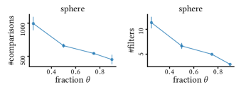
(a)

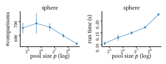
(b)

Figure 6. Effect of parameters on algorithm List-QP

D.1. Effect of parameters

Recall that in Algorithm 1, a pool $P$ of $p$ tuples is used to test the performance of a new filter. A new filter will be ready when it can prune at least a $\theta$ fraction of tuples in $P$. In Fig. 6, we run Algorithm 1 with a List-QP filter on a dataset of 10k tuples. We fix one parameter ($p=100$ or $\theta=0.5$) and vary the other.

Parameter $\theta$ roughly specifies the expected fraction of tuples a filter should be able to prune. A larger $\theta$ implies a need for fewer filters but a larger sample size for each filter. It is beneficial to use a large $\theta$ which leads a smaller number of comparisons overall. Nevertheless, as we will see shortly, such a large filter can be time-consuming to run, especially when the dimension $d$ is large.

A larger value of $p$ improves the reliability of the testbed $P$, which helps reducing the number of comparisons. However, a larger $p$ also results in longer time to run filters over the testbed $P$.