Generalized Lotka-Volterra Systems with Time Correlated Stochastic Interactions

Abstract

The dynamics of species communities are typically modelled considering fixed parameters for species interactions. The problem of over-parameterization that ensues when considering large communities has been overcome by sampling species interactions from a probability distribution. However, species interactions are not fixed in time, but they can change on a time scale comparable to population dynamics. Here we investigate the impact of time-dependent species interactions using the generalized Lotka-Volterra model, which serves as a paradigmatic theoretical framework in several scientific fields. In this work we model species interactions as stochastic colored noise. Assuming a large number of species and a steady state, we obtain analytical predictions for the species abundance distribution, which matches well empirical observations. In particular, our results suggest the absence of extinctions, unlike scenarios with fixed species interactions.

I Introduction

In the last years, the approach of statistical physics has been decisively contributing to our understanding of ecological processes by providing powerful theoretical tools and innovative steps towards the comprehension and the synthesis of broad empirical evidence [1], especially in microbial ecology [2, 3, 4, 5]. In fact, the advent of next-generation sequencing techniques is generating an increasing volume of ecologically relevant data, characterizing several microbial communities in different environments and involving a large number of species [6, 7]. For this reason, the theoretical approach has shifted from the traditional dynamical systems theory, which is effectively used for a small number of species [8, 9], to statistical physics-based methods that are better suited for large systems [10, 11, 12, 13, 14]. In particular, several recent works have proposed to model species interactions through Generalized Lotka-Volterra equations with quenched random disorder (QGLV), and this approach has yielded a number of interesting results [15, 16, 17, 18]. The phase diagram of these models describe a system which transitions from a single stationary state to an unbounded one, passing through a multiple-attractors state as the variance of the interactions between species exceeds a critical value [19, 16]. Furthermore, with the addition of demographic noise to the QGLV new phases are also found such as a Gardner phase [20].

The QGLV does not typically display properties observed by real ecosystems. It suffers from the stability-diversity paradox [21, 22, 23], which for QGLV emerges as a result of a dynamical process where the system reduces the number of coexisting species so to remain marginally stable [16]. Moreover, the species abundance distribution (SAD), as obtained in the limit of a large number of species within the dynamical mean field theory (DMFT) or cavity method, is a truncated Gaussian [19, 17], very different from the heavy tail SAD observed in empirical microbial [24, 25, 4] or in forest communities [26].

Another limitation of the QGLV model is its underlying assumption that species interactions remain constant over time. However, ecological systems in reality are characterized by temporal fluctuations in species interactions, influenced by variations in environmental conditions, resource availability, and other factors which operate on a timescale that is comparable to the population dynamics [27, 28, 29, 30].

In the present study, we explicitly consider time-dependent species interactions as an alternative approach. Specifically, we adopt the hypothesis that these interactions can be modeled as stochastic colored noises within the framework of the GLV model, which we will call annealed GLV (AGLV). Strikingly, the introduction of temporal stochastic fluctuations in the strengths of species interactions yields results that are remarkably rich and ecologically relevant. By employing the DMFT in the limit of a large number of species, we analytically determine the stationary state, which is in excellent agreement with numerical simulations of the AGLV. In the case of white noise limit, the resulting SAD is a Gamma distribution, in agreement with observed distributions in plant and microbial communities [26, 24]. Moreover, this also justifies a recently introduced phenomenological model [4, 31, 32] that has been shown to reproduce several macro-ecological laws, thus providing further validation and support for our approach. Eventually, we study the AGLV phase diagram which reveals two distinct phases: one where the system reaches a stationary state and all species coexist; another one where unbounded growth is observed.

Let us consider $x_{i}(t)$, the population at time $t$ of the species $i$. Then the dynamics of the AGLV system with colored noise for $S$ interacting species are given by

$$\dot{x}_{i}(t)=r_{i}x_{i}(t)\big{[}1-x_{i}(t)/K_{i}+\sum_{j\neq i}\alpha_{ij}(t)x_{j}(t)+h_{i}(t)\big{]},$$ (1)

with $i=1,...,S$, and where $\alpha_{ij}(t)=\mu/S+\sigma z_{ij}(t)/\sqrt{S}$ for $i\neq j$ and $\{z_{ij}(t):t>0\}$ are independent Gaussian random variables with $\overline{z_{ij}(t)}=0$, $\overline{z_{ij}(t)z_{ij}(t^{\prime})}=P(\Delta t|\tau)=\frac{1+2\tau/\tau_{0}}{2\tau}e^{-\Delta t/\tau}$, where $\Delta t=|t-t^{\prime}|$; $h_{i}(t)$ is a possible time dependent external field. For simplicity, we set $\tau_{0},r_{i},K_{i}=1$ for $i=1,...,S$ and we work with dimensionless variables/parameters. From this general annealed formulation with colored noise, the limit $\tau\rightarrow 0$ corresponds to the white noise (AWN) dynamics. In Fig. 1 we show the effect of time correlated noise in the species abundances evolution. Our proposed model presents a distinct characteristic, where species populations undergo recurring quasi-cycles of both high and low abundances, whose average frequency depends on the value of $\tau$. This cyclic behavior is instrumental in promoting the coexistence of multiple species within the ecosystem (as also noted in [18, 33]), and it is present for all ranges of $\tau$, including the limit $\tau\rightarrow 0$.

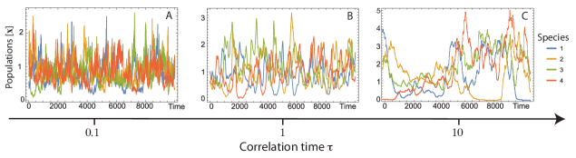
Figure 1: Examples of four species abundances trajectories obtained by simulating eq. (1) for $S=30$, $h=\gamma=0$ and different values of the characteristic correlation time $\tau$. A) $\tau=0.1$, $\mu=0$, $\sigma=1$, the dynamics is basically the one corresponding to the white noise case ($\tau=0$); B) $\tau=1$, $\mu=0$, $\sigma=0.8$, the time correlations start to play a role in the species dynamics; C) $\tau=10$, $\mu=0$, $\sigma=0.6$ species populations alternate long periods of high and low abundance similarly to what observed in the classic quenched multi-attractors regime.

The DMFT for the general AGLV eq. (1) is given by (see Supplementary Methods)

$$\dot{x}(t)=x(t)\big{[}1-x(t)+\mu M(t)+\sigma\eta(t)+h(t)\big{]},$$ (2)

where $M(t)=\mathrm{E}(x(t))$ and in the following we set $h(t)=0$.

The self-consistent Gaussian noise $\eta(t)$ is such that $\mathrm{E}(\eta(t))=0$ and $\mathrm{E}(\eta(t)\eta(t^{\prime}))=P(\Delta t|\tau)\mathrm{E}(x(t)x(t^{\prime}))$. From Fig. (3) we can see that at stationarity, the (connected) auto-correlation function of $x(t)$ decays exponentially

$$\mathrm{E}(x(t)x(t^{\prime}))-\mathrm{E}^{2}(x)=\big{(}\mathrm{E}({x}^{2})-\mathrm{E}^{2}(x)\big{)}e^{-\frac{|\Delta t|}{\tau_{x}}},$$ (3)

and exploiting eq. (3) we can simplify the self consistency for $\eta$ as $\mathrm{E}(\eta(t)\eta(t^{\prime}))=P(\Delta t|\bar{\tau})\mathrm{E}({x}^{2})$, at least in the relevant regime $|t-t^{\prime}|\ll\tau_{x}$, with the new effective time scale $\bar{\tau}=1/\big{[}1/\tau+\big{(}1-\mathrm{E}^{2}(x)/\mathrm{E}({x}^{2})\big{)}/\tau_{x}\big{]}$ (see Supplementary Methods for further details). With this simplification we can now use the Unified Colored Noise Approximation (UCNA) [34] on eq. (2), which leads to the stationary SAD

$$P_{\tau}^{*}(x)=\frac{x^{-1+\delta_{\tau}}}{Z}\left(\frac{1}{\bar{\tau}}+x\right)e^{-\frac{x}{D}-\frac{\bar{\tau}}{2D}(x-\bar{x})^{2}},$$ (4)

where $x>0$, $Z$ is the normalization constant, that can be computed analytically, $\delta_{\tau}=(1+\mu M^{*})/D(\tau)$, $D(\tau)=\sigma^{2}\mathrm{E^{*}}(x^{2})(1+2\tau)\bar{\tau}(\tau)/2\tau$ and $\bar{x}=1+\mu M^{*}$ ($\mathrm{E^{*}}(\cdot)$ denotes the average with the distribution $P_{\tau}^{*}$ and $M^{*}=\mathrm{E^{*}}(x)$). As anticipated, we thus find that for all finite $\tau$ no extinction occurs as also confirmed by numerically integrating eq. (1) for 30 species (see Fig. 2). Notice that $P_{\tau}^{*}(x)$ is basically an interpolation between a truncated Gaussian ( peaked at $x>0$) and a Gamma distribution. The former is known to be the solution for the SAD of the DMFT in the case of random quenched interactions in the single equilibrium phase [19, 17], while the latter we will show is the exact solution of the AWN case, corresponding to the limit $\bar{\tau}\sim\tau\rightarrow 0$ of eq. (2). In the AWN limit, in fact, the DMFT equation is the same of eq. (2), but in this case with $\mathrm{E}(\eta(t)\eta(t^{\prime}))=\Sigma^{2}(t)\delta(t-t^{\prime})$, $\Sigma^{2}(t)=\mathrm{E}(x^{2}(t))$, and the multiplicative noise term $x(t)\eta(t)$ should be interpreted in the Stratonovich sense [35]. At stationarity, the self-consistency imposes $M^{*}=\mathrm{E^{*}}(x)$ and ${\Sigma^{*}}^{2}=\mathrm{E^{*}}(x^{2})$. The exact stationary distribution $P_{0}^{*}$ can be derived from the Fokker-Planck Equation corresponding to eq. (2) and it reads

$$P_{0}^{*}(x)=\frac{\beta^{\delta}}{\Gamma(\delta)}x^{-1+\delta}e^{-\beta x},$$ (5)

and it coincides with the limits of $P_{\tau}^{*}(x)$ when $\tau\to 0$. We also have that $\lim_{\tau\rightarrow 0}\delta_{\tau}=2(1+\mu M^{*})/(\sigma^{2}{\Sigma^{*}}^{2})\equiv\delta$ with $M^{*}=1/(1-\mu)$ and ${\Sigma^{*}}^{2}=\delta(\delta+1)/\beta^{2}$. In this way we can write explicitly the SAD’s parameters as a function of $\mu$ and $\sigma$ as (see Supplementary Methods):

$$\beta=\frac{\sigma^{2}}{2}\delta(\delta+1);\quad\delta=\frac{2}{\sigma^{2}}(1-\mu)-1.$$ (6)

The histograms in Figure 2 show the probability distributions for the stationary species abundances obtained by simulating the full AGLV equations given by eq. (1) for the same parameters used in Fig. 1. The predicted SADs by the DMFT are plotted as continuous lines and given, respectively, by eq. (4) and in (A) also by eq. (5), denoted by the dark blue dashed line. In the latter case, the distribution parameters are directly calculated from eq. (6) as a function of $\mu$ and $\sigma$. For eq. (4) instead, the parameters are obtained by first fitting the distribution and then checking the agreement with the self-consistent equations (error below $5\%$, see Supplementary Methods).

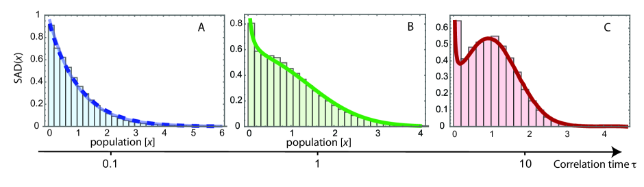
Figure 2: The histograms represent the Species Abundance Distributions (SADs) obtained by simulating the full AGLV system given by eq. (1), while the continuous lines are the corresponding SADs given by the DMFT A) of both the colored case eq. (4) with $\tau=0.1$ and the white noise Annealed case given by eq. (5); B-C) Colored noise AGLV (eq. (4)) with $\tau=1$ and $\tau=10$, respectively. The analytical DMFT perfectly describes the SAD given by the numerical simulations of the full system simulated for S=30 species. Initial conditions of the populations in all cases are drawn from $x_{i}\sim U[0.1,0,2]$, where $U$ denotes the uniform distribution, while the value $\mu$ and $\sigma$ is as in Fig. 1.

Using the chosen value of the correlation time, $\tau$, the parameters $D(\tau)$ and $\bar{\tau}(\tau)$ given by our analytical framework, we can deduce the value of $\tau_{x}$ in eq. (3). The red line in Figure 3 shows that indeed the predicted value of $\tau_{x}$ is consistent with the decay of $\mathrm{E}(x(t))(x(t^{\prime}))$ obtained by simulating the full AGLV system given by eq. (1) (error below $5\%$, see Supplementary Methods).

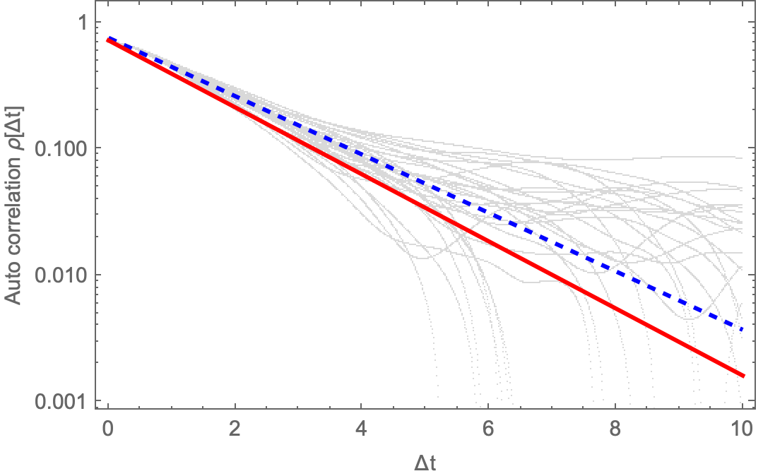
Figure 3: Gray lines represent the empirical autocorrelation function calculated as $\mathrm{E}(x(t)x(t+\Delta t))-\mathrm{E}^{2}(x)$ (averaged over $t$) for each of the $S=30$ species simulated using the AGLV with $\tau=1$ ($\mu=0$ and $\sigma=0.8$. The blue dashed line represents the exponential fit, while the thick red line represent the exponential decay given by the ansatz eq. (3) using the parameters obtained from $P^{*}(x)$ in Fig. 2B.

Since $\delta>0$ and $\mathrm{E}(x)>0$, in order for the stationary solution to exist, we have the conditions $\sigma<\sqrt{2(1-\mu)}$ and $\mu\leq 1$, leading to a lower bound for the unbounded growth phase of the AGLV as shown in Fig. 4. However, by solving numerically the self-consistent eq. (2) (see Supplementary Methods) and also performing the numerical simulation of the entire GLV systems, we find that below this bound, even though a stationary solution exists, it may not be reached. In particular, in the red region of Fig. 4, independently of the initial condition for $x(t=0)$, there is a singularity at finite times, leading to the explosion of the species population. In the green region instead, if we start close to the predicted stationary solution $P^{*}(x)$, then we always find that the stationary solution is reached and it coincides with the one predicted by the DMFT eq. (5). However, there is a set of initial conditions (for sufficiently large $x(t=0)$) for which $x(t)$ may diverge for finite $t$. Such divergent trajectories are also confirmed when we simulate the full eq. (1) for a large enough number of species (see Supplementary Methods). However, understanding the divergence at finite times due to the non-linearity of the Fokker-Planck equation and its dependence on initial conditions is left for future works

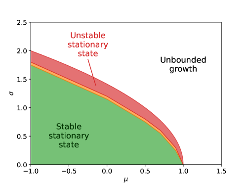
Figure 4: Phase Space Diagram for the annealed white noise case. We show the AGLV dynamics as a function of the mean ($\mu$) and the standard deviation ($\sigma$) of the species’ interaction strengths. In the unbounded region, as predicted analytically, the species abundance dynamics diverge for finite times. In the red region, although the stationary solution of the DMFT equation exists, it is not reachable by the dynamics and also here we have a singularity for finite times. In the green region, for initial conditions taken from the stationary distribution eq. (5), a stationary state exists and it corresponds to the Gamma distribution as given by eq. (5). In orange the region of numerical uncertainty.

In this study, we have undertaken an investigation into the GLV equations with annealed disorder, incorporating finite correlation time, and have determined the corresponding dynamical mean field for a large number of species. The inclusion of temporal stochastic fluctuations in the strengths of species interactions has resulted in a remarkably diverse range of phenomena and ecologically significant outcomes. Firstly, the introduction of annealed disorder in the GLV equations, for any finite correlation time, has exerted a substantial positive influence on the biodiversity of the system. Specifically, when the dynamics of the system converge to the stationary distribution, we observe the coexistence of all species without extinctions. This is not the case in conventional quenched GLV models where extinctions are observed [19, 16, 17, 37]. The facilitation of coexistence arises from the existence of temporal periods during which species abundances alternate between high and low values. This phenomenon engenders favorable conditions for the persistence of species and prevents their local extinctions. Second, in the white noise limit, the DMFT leads to the stochastic logistic model, a phenomenological model that proved to be consistent with several macro-ecological laws in microbial ecosystems [4]. In particular, the analytical species abundance distribution derived from the DMFT follows the Gamma distribution, a widely utilized probability distribution in macro-ecology [26, 1]. Furthermore, we have successfully obtained the phase diagram for the case of annealed white noise (AWN), and numerical simulations have revealed the potential for unbounded growth when the initial conditions possess large values, despite the existence of an analytically stationary solution. In other words, due to the non-linear nature of the corresponding Fokker-Planck equation, the dynamics may not converge to the stationary solution, leading to divergent trajectories. Our future work will focus on conducting more detailed analyses to explore the nature of these finite time singularities. Moreover, we propose various other avenues of research, including the integration of quenched as well as annealed disorder and the correlations between pairs of interacting species [19, 17] or more complex hierarchical correlation structures [38] More generally, the methodology presented here can be exploited to study the effect of annealed disorder also in other ecological dynamics.

The exploration of such directions within our framework holds significant promise for advancing the modelling of large-scale ecosystem dynamics, understanding emergent macro-ecological patterns observed in empirical data, and investigating the influence of environmental fluctuations on species coexistence.