Measurement of $\boldsymbol{C\!P}$ asymmetries in $\boldsymbol{B^{0}\rightarrow\phi K^{0}_{S}}$ decays with Belle II

Abstract

We present a measurement of time-dependent rate asymmetries in $B^{0}\rightarrow\phi K^{0}_{S}$ decays to search for non-standard-model physics in $b\rightarrow q\overline{}qs$ transitions. The data sample is collected with the Belle II detector at the SuperKEKB asymmetric-energy $e^{+}e^{-}$ collider in 2019–2022 and contains $(387\pm 6)\times 10^{6}$ bottom-antibottom mesons from $\mathchar 28935\relax{(4S)}$ resonance decays. We reconstruct $162\pm 17$ signal events and extract the charge-parity ($C\!P$) violating parameters from a fit to the distribution of the proper-decay-time difference of the two $B$ mesons. The measured direct and mixing-induced $C\!P$ asymmetries are $\comment{C}=\comment{-0.31\pm 0.20\pm 0.05}$ and $S=0.54\pm 0.26^{+0.06}_{-0.08}$, respectively, where the first uncertainties are statistical and the second are systematic. The results are compatible with the $C\!P$ asymmetries observed in $b\rightarrow c\overline{}cs$ transitions.

I Introduction

Measurements of $C\!P$ asymmetries in loop-suppressed $B$ meson decays are sensitive probes of physics beyond the standard model (SM). In particular, gluonic-penguin $b\rightarrow q\overline{}qs$ modes, such as $B^{0}\rightarrow\phi K^{0}_{S}$, are sensitive to interfering non-SM amplitudes that carry additional weak-interaction phases. The SM reference is the mixing-induced $C\!P$ asymmetry $S\equiv\sin 2\phi_{1}$ observed in tree-level $b\rightarrow c\overline{}cs$ transitions, where $\phi_{1}$ (or $\beta$) equals $\arg(-V_{cd}V_{cb}^{*}/V_{td}V_{tb}^{*})$ and $V_{ij}$ are Cabibbo-Kobayashi-Maskawa (CKM) quark-mixing matrix elements Cabibbo (1963); Kobayashi and Maskawa (1973). The deviation from the value of $S$ observed in $b\rightarrow c\overline{}cs$ transitions, $S=0.699\pm 0.017$ Amhis et al. (2023), is the key observable. For $B^{0}\rightarrow\phi K^{0}_{S}$ decays, such a deviation is at most $0.02\pm 0.01$ within the SM while the direct $C\!P$ asymmetry $C$ is expected to be zero Beneke (2005). The current world-average values for $B^{0}\rightarrow\phi K^{0}_{S}$ are $S=0.74^{+0.11}_{-0.13}$ and $\comment{C}=0.01\pm 0.14$ Amhis et al. (2023). Therefore, experimental knowledge must be improved. We present a measurement of $S$ and $C$ in the sample of electron-positron collisions collected by the Belle II experiment in 2019–2022 cp- .

At $B$-factories, $B\kern 1.79993pt\overline{\kern-1.79993ptB}{}$ events are produced from the decay of an $\mathchar 28935\relax{(4S)}$ resonance, where $B$ indicates a $B^{+}$ or $B^{0}$ meson. We denote pairs of neutral $B$ mesons as $B_{C\!P}B_{\text{tag}}$, where $B_{C\!P}$ decays into a $C\!P$-eigenstate at time $t_{C\!P}$, and $B_{\text{tag}}$ decays into a flavor-specific final state at time $t_{\text{tag}}$. For quantum-correlated $B$-meson pairs, the flavor of $B_{C\!P}$ is opposite to that of $B_{\text{tag}}$ at the instant when the $B_{\text{tag}}$ decays. The probability to observe a $B_{\text{tag}}$ meson with flavor $q$ ($q=+1$ for $B^{0}$ and $q=-1$ for $\kern 1.79993pt\overline{\kern-1.79993ptB}{}^{0}$) and a proper-time difference $\Delta t\equiv t_{C\!P}-t_{\text{tag}}$ between the $B_{C\!P}$ and $B_{\text{tag}}$ decays is

$$\begin{split}\mathcal{P}(\Delta t,q)=\frac{e^{-|\Delta t|/\tau_{B^{0}}}}{4\tau_{B^{0}}}\Big{\{}1+q\big{[}&S\sin(\Delta m_{d}\Delta t)\\ -&\comment{C}\cos(\Delta m_{d}\Delta t)\big{]}\Big{\}},\end{split}$$ (1)

where $\tau_{B^{0}}$ and $\Delta m_{d}$ are the $B^{0}$ lifetime and $B^{0}-\kern 1.79993pt\overline{\kern-1.79993ptB}{}^{0}$ mixing frequency, respectively Workman et al. (2022).

We reconstruct $B^{0}\rightarrow\phi K^{0}_{S}$ decays in a sample of energy-asymmetric $e^{+}e^{-}$ collisions at the $\mathchar 28935\relax{(4S)}$ resonance provided by SuperKEKB and collected with the Belle II detector. The sample corresponds to $(362\pm 2)\leavevmode\nobreak\ \mbox{\,fb}^{-1}$ and contains $(387\pm 6)\times 10^{6}$ $B\kern 1.79993pt\overline{\kern-1.79993ptB}{}$ events. We fully reconstruct $B_{C\!P}$ in the $\phi K^{0}_{S}$ final state using the intermediate decays $\phi\rightarrow K^{+}K^{-}$ and $K^{0}_{S}\rightarrow\pi^{+}\pi^{-}$, while we only determine the position of the $B_{\text{tag}}$ decay. The flavor of the $B_{\text{tag}}$ meson is inferred from the properties of all charged particles in the event not belonging to $B_{C\!P}$ Abudinén et al. (2022). In order to extract the $C\!P$ asymmetries, we model the distributions of signal $B_{C\!P}$ and backgrounds in $\Delta t$ and other discriminating variables, and then perform a likelihood fit. The last measurements, by the Belle and BABAR experiments, used time-dependent Dalitz-plot analyses Nakahama et al. (2010); Lees et al. (2012). This method models the interferences among the intermediate resonant and nonresonant amplitudes contributing to $B^{0}\rightarrow K^{+}K^{-}K^{0}_{S}$ decays, thereby providing the best sensitivity on $\phi_{1}$. Due to the small dataset size, which may induce multiple solutions in the Dalitz-plot approach, we perform a quasi-two-body analysis by restricting the sample to candidates reconstructed in a narrow region around the $\phi$ mass. This strategy offers the advantage of a simpler analysis, albeit with a reduced statistical sensitivity. We use the knowledge from the previous Dalitz-plot analyses to estimate the effect of neglecting the interferences. We test our analysis on the $C\!P$-conserving $B^{+}\rightarrow\phi K^{+}$ decay, which has similar backgrounds and vertex resolution. Charge-conjugated modes are included throughout the paper.

II Experimental setup

The Belle II detector Abe et al. operates at the SuperKEKB accelerator at KEK, which collides 7 $\mathrm{\,Ge\kern-1.00006ptV}$ electrons with 4 $\mathrm{\,Ge\kern-1.00006ptV}$ positrons. The detector is designed to reconstruct the decays of heavy-flavor mesons and $\tau$ leptons. It consists of several subsystems arranged cylindrically around the interaction point (IP). The innermost part of the detector is equipped with a two-layer silicon-pixel detector (PXD), surrounded by a four-layer double-sided silicon-strip detector (SVD) Adamczyk et al. (2022). Together, they provide information about charged-particle trajectories (tracks) and decay-vertex positions. Of the outer PXD layer, only one-sixth is installed for the data used in this work. The momenta and electric charges of charged particles are determined with a 56-layer central drift-chamber (CDC). Charged-hadron identification (PID) is provided by a time-of-propagation counter and an aerogel ring-imaging Cherenkov counter, located in the central and forward regions outside the CDC, respectively. The CDC provides additional PID information through the measurement of specific ionization. Photons are identified and electrons are reconstructed by an electromagnetic calorimeter made of CsI(Tl) crystals, covering the region outside of the PID detectors. The tracking and PID subsystems, and the calorimeter, are surrounded by a superconducting solenoid, providing an axial magnetic field of 1.5 T. The central axis of the solenoid defines the $z$ axis of the laboratory frame, pointing approximately in the direction of the electron beam. Outside of the magnet lies the muon and $K^{0}_{L}$ identification system, which consists of iron plates interspersed with resistive-plate chambers and plastic scintillators.

We use simulated events to model signal and background distributions, study the detector response, and test the analysis. Quark-antiquark pairs from $e^{+}e^{-}$ collisions, and hadron decays, are simulated using KKMC Jadach et al. (2000) with Pythia8 Sjöstrand et al. (2015), and EvtGen Lange (2001), respectively. The detector response and $K^{0}_{S}$ decays are simulated using Geant4 Agostinelli et al. (2003). Collision data and simulated samples are processed using the Belle II analysis software Kuhr et al. (2019); bas .

III Event reconstruction

Events containing a $B\kern 1.79993pt\overline{\kern-1.79993ptB}{}$ pair are selected online by a trigger based on the track multiplicity and total energy deposited in the calorimeter. We reconstruct $B^{0}\rightarrow\phi K^{0}_{S}$ decays using $\phi\rightarrow K^{+}K^{-}$ and $K^{0}_{S}\rightarrow\pi^{+}\pi^{-}$ decays, in which the four tracks are reconstructed using information from the PXD, SVD, and CDC Bertacchi et al. (2021). All tracks are required to have polar angle $\theta$ within the CDC acceptance ($17^{\circ}<\theta<150^{\circ}$). Tracks used to form $\phi$ candidates are required to have a distance of closest approach to the IP less than $2.0$ $\rm\,cm$ along the $z$ axis and less than $0.5$ $\rm\,cm$ in the transverse plane to reduce contamination of tracks not generated in the collision.

Kaon and pion mass hypotheses are assigned to tracks based on information provided by the PID subsystems. The $\phi$ candidates are formed by combining $K^{+}K^{-}$ pairs consistent with originating from the IP and having invariant mass within $[0.99,1.09]$ ${\mathrm{\,Ge\kern-1.00006ptV\!/}c^{2}}$, where the average $\phi$ mass resolution is approximately 3 ${\mathrm{\,Me\kern-1.00006ptV\!/}c^{2}}$. The $K^{0}_{S}$ candidates are formed by combining two oppositely charged particles, assumed to be pions, and requiring their invariant mass to be within $[0.480,0.515]$ ${\mathrm{\,Ge\kern-1.00006ptV\!/}c^{2}}$, where the average $K^{0}_{S}$ mass resolution is approximately 2 ${\mathrm{\,Me\kern-1.00006ptV\!/}c^{2}}$. In order to suppress combinatorial background from misreconstructed $K^{0}_{S}$, we require $K^{0}_{S}$ candidates to have a displacement of at least 0.05 $\rm\,cm$ from the $\phi$ decay vertex, where the average $K^{0}_{S}$ flight distance is 10 $\rm\,cm$.

The beam-energy constrained mass $M_{\text{bc}}$ and energy difference $\Delta E$ are computed for each $B^{0}\rightarrow\phi K^{0}_{S}$ candidate as $M_{\text{bc}}\equiv\sqrt{(E_{\text{beam}}^{*}/c^{2})^{2}-(|p_{B}^{*}|/c)^{2}}$ and $\Delta E\equiv E_{B}^{*}-E_{\text{beam}}^{*}$, where $E_{\text{beam}}^{*}$ is the beam energy, and $E_{B}^{*}$ and $p_{B}^{*}$ are the energy and momentum of the $B_{C\!P}$ candidate, respectively, all calculated in the center-of-mass (c.m.) frame. Signal $B_{C\!P}$ candidates peak at the known $B^{0}$ mass Workman et al. (2022) and zero in $M_{\text{bc}}$ and $\Delta E$, respectively, while continuum is distributed more uniformly. Only candidates satisfying $M_{\text{bc}}>5.2\leavevmode\nobreak\ {\mathrm{\,Ge\kern-1.00006ptV\!/}c^{2}}$ and $|\Delta E|<0.2\leavevmode\nobreak\ \mathrm{\,Ge\kern-1.00006ptV}$ are retained for further analysis.

The $B^{0}\rightarrow\phi K^{0}_{S}$ decay vertex is determined using the TreeFitter algorithm Hulsbergen (2005); Krohn et al. (2020). In addition, the $B_{C\!P}$ candidate is constrained to point back to the IP. The $B_{\text{tag}}$ decay vertex is reconstructed using the remaining tracks in the event. Each track is required to have at least one measurement point in the SVD and CDC subdetectors and correspond to a total momentum greater than 50 ${\mathrm{\,Me\kern-1.00006ptV\!/}c}$. The $B_{\text{tag}}$ decay-vertex position is fitted using the Rave algorithm Waltenberger et al. (2008), which allows for weighting the contributions from tracks that are displaced from the $B_{\text{tag}}$ decay vertex, and thereby suppressing biases from secondary charm decays. The decay-vertex position is determined by constraining the $B_{\text{tag}}$ direction, as determined from its decay vertex and the IP, to be collinear with its momentum vector Dey and Soffer (2020).

We estimate the proper-time difference using the longitudinal decay-vertex positions, $\ell_{C\!P}$ and $\ell_{\text{tag}}$, of the $B_{C\!P}$ and $B_{\text{tag}}$ mesons, respectively, as

$$\Delta t\approx\frac{\ell_{C\!P}-\ell_{\text{tag}}}{\beta\gamma\gamma^{*}c},$$ (2)

where $\beta\gamma=0.28$ is the $\mathchar 28935\relax{(4S)}$ Lorentz boost and $\gamma^{*}=1.002$ is the Lorentz factor of the $B$ mesons in the c.m. frame. The average distance between the $B_{C\!P}$ and $B_{\text{tag}}$ vertices is approximately 100 µm along the $z$ axis. The $B$-decay vertex resolution along the $z$ axis is approximately 35 µm for simulated $B^{0}\rightarrow\phi K^{0}_{S}$ decays. We apply loose $\chi^{2}$ probability requirements to both the $B_{C\!P}$ and $B_{\text{tag}}$ vertices. Events having a $\Delta t$ uncertainty $\sigma_{\Delta t}$ greater than $2.0$ ${\rm\,ps}$, where the average value is approximately 0.5 ${\rm\,ps}$, are not included in the analysis, as they constitute less than 2% of the signal events and do not contribute to the determination of $S$.

The dominant sources of background come from continuum $e^{+}e^{-}\rightarrow q\overline{}q$ events, where $q$ indicates a $u$, $d$, $c$, or $s$ quark. A boosted-decision-tree (BDT) classifier is trained on simulated samples to combine several topological variables that provide separation between continuum and signal events Chen and Guestrin (2016). The variables included in the BDT are the following, in order of decreasing discriminating power: the cosine of the angle between the thrust axes of $B_{C\!P}$ and $B_{\text{tag}}$ Ed. A. J. Bevan, B. Golob, Th. Mannel, S. Prell, and B. D. Yabsley (2014), the modified Fox-Wolfram moments introduced in Ref. Lee et al. (2003), the thrust of $B_{\text{tag}}$ Brandt et al. (1964); Farhi (1977), the ratio of the zeroth to the first Fox-Wolfram moment Fox and Wolfram (1978), and the harmonic moments calculated with respect to the thrust axis. We impose a minimum requirement on the output of the BDT, $\mathcal{O}_{\text{CS}}$, that retains more than $95\%$ of the signal, while rejecting more than 55% of the continuum events. The transformed output of the classifier, defined as $\mathcal{O}^{{}^{\prime}}_{\text{CS}}=\log[(\mathcal{O}_{\text{CS}}-\mathcal{O}_{\text{CS}}^{\text{min}})/(\mathcal{O}_{\text{CS}}^{\text{max}}-\mathcal{O}_{\text{CS}})]$, where $\mathcal{O}_{\text{CS}}^{\text{min}}$ and $\mathcal{O}_{\text{CS}}^{\text{max}}$ are the minimum and maximum values of the selected events, is included in the fit. The signal and remaining background events are approximately Gaussian-distributed in this variable and are therefore simple to model.

An additional requirement $|\Delta E|<50\leavevmode\nobreak\ \mathrm{\,Me\kern-1.00006ptV}$ further suppresses continuum and misreconstructed $B\rightarrow\phi K^{*}$ decays. To reduce the contamination from nonresonant $B^{0}\rightarrow K^{+}K^{-}K^{0}_{S}$ decays and other modes leading to the same final state, events are required to satisfy $|m(K^{+}K^{-})-m_{\phi}|<10{\mathrm{\,Me\kern-1.00006ptV\!/}c^{2}}$, where $m_{\phi}$ is the known $\phi$ meson mass Workman et al. (2022).

The same event reconstruction is applied on $B^{+}\rightarrow\phi K^{+}$ decays, except for the $K^{0}_{S}$ selection, which is replaced by a $K^{+}$ track with a stringent PID requirement. This is more than $90\%$ efficient on the signal, while rejecting around $30\%$ of misidentified charged particles. We achieve a total signal reconstruction efficiency of $33$% for $B^{0}\rightarrow\phi K^{0}_{S}$ and $40$% for $B^{+}\rightarrow\phi K^{+}$.

Events with multiple candidates account for approximately 6% of the data. We keep the candidate with the highest $B_{C\!P}$ vertex $\chi^{2}$ probability. The criterion retains the correct signal candidate 67% of the times using simulated events. We check that the candidate selection does not bias the $\Delta t$ distribution by comparing the results of lifetime fits to the $B^{0}$ and $B^{+}$ samples with known values Workman et al. (2022).

IV Time-dependent $C\!P$-asymmetry fit

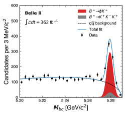
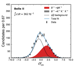
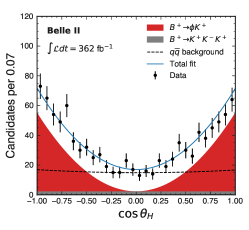
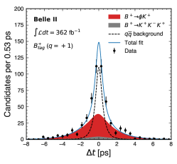
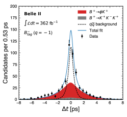
Figure 1: Distributions of (top left) $M_{\text{bc}}$, (top center) $\mathcal{O}^{{}^{\prime}}_{\text{CS}}$, (top right) $\cos\theta_{H}$, (bottom left) $\Delta t$ for $B^{+}$-tagged and (bottom right) $\Delta t$ for $B^{-}$-tagged $B^{+}\rightarrow\phi K^{+}$ candidates (data points) with fits overlaid (curves and stacked shaded areas). The $M_{\text{bc}}$ distribution is displayed for candidates with $\mathcal{O}^{{}^{\prime}}_{\text{CS}}>-1$ and the $\mathcal{O}^{{}^{\prime}}_{\text{CS}}$ distribution is displayed for candidates with $M_{\text{bc}}>5.27$ ${\mathrm{\,Ge\kern-1.00006ptV\!/}c^{2}}$. The $\cos\theta_{H}$ and $\Delta t$ distributions are displayed for candidates with $\mathcal{O}^{{}^{\prime}}_{\text{CS}}>-1$ and $M_{\text{bc}}>5.27$ ${\mathrm{\,Ge\kern-1.00006ptV\!/}c^{2}}$.

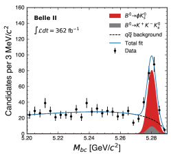
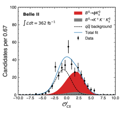
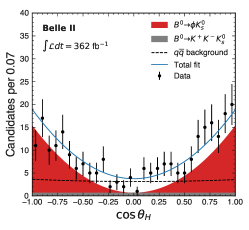
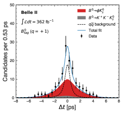
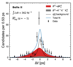
Figure 2: Distributions of (top left) $M_{\text{bc}}$, (top center) $\mathcal{O}^{{}^{\prime}}_{\text{CS}}$, (top right) $\cos\theta_{H}$, (bottom left) $\Delta t$ for $B^{0}$-tagged and (bottom right) $\Delta t$ for $\kern 1.79993pt\overline{\kern-1.79993ptB}{}^{0}$-tagged $B^{0}\rightarrow\phi K^{0}_{S}$ candidates (data points) with fits overlaid (curves and stacked shaded areas). The $M_{\text{bc}}$ distribution is displayed for candidates with $\mathcal{O}^{{}^{\prime}}_{\text{CS}}>-1$ and the $\mathcal{O}^{{}^{\prime}}_{\text{CS}}$ distribution is displayed for candidates with $M_{\text{bc}}>5.27$ ${\mathrm{\,Ge\kern-1.00006ptV\!/}c^{2}}$. The $\cos\theta_{H}$ and $\Delta t$ distributions are displayed for candidates with $\mathcal{O}^{{}^{\prime}}_{\text{CS}}>-1$ and $M_{\text{bc}}>5.27$ ${\mathrm{\,Ge\kern-1.00006ptV\!/}c^{2}}$.

The distributions of signal and backgrounds are described in a likelihood fit to extract the $C\!P$ asymmetries. We consider the following contributions to the sample composition: signal $B^{0}\rightarrow\phi K^{0}_{S}$ events, nonresonant $B^{0}\rightarrow K^{+}K^{-}K^{0}_{S}$ background, and continuum background. Additional $B\kern 1.79993pt\overline{\kern-1.79993ptB}{}$ background events are treated as a source of systematic uncertainty, as they are estimated to be at most 2% of the signal yield, according to simulation. Low-multiplicity events contribute at less than the level of the $B\kern 1.79993pt\overline{\kern-1.79993ptB}{}$ backgrounds in the simulation, and are distributed like continuum in the variables used in the fit, so they are treated as part of the continuum background. We model the distributions of signal and background events in the $M_{\text{bc}}$, $\mathcal{O}^{{}^{\prime}}_{\text{CS}}$, $\cos\theta_{H}$, and $\Delta t$ variables. The $M_{\text{bc}}$ and $\mathcal{O}^{{}^{\prime}}_{\text{CS}}$ variables provide discrimination between signal and continuum background. The helicity angle $\theta_{H}$, defined as the angle between the momentum of the $B^{0}$ and that of the positively charged kaon in the $\phi$ rest frame, is used to distinguish between signal and nonresonant components. The $\Delta t$ variable and tag-flavor $q$ provide access to the time-dependent $C\!P$ asymmetries. In addition, we use $\sigma_{\Delta t}$ as a conditional observable to model the per-event resolution.

We extract the $C\!P$ asymmetries using an extended maximum-likelihood fit to the unbinned distributions of the discriminating variables. The total probability density function (PDF) is given by the product of the four one-dimensional PDFs, since the dependences among the fit observables are negligible. We model the $M_{\text{bc}}$ distribution using an ARGUS function Albrecht et al. (1990) for continuum and a Gaussian function with shared parameters for the $B^{0}\rightarrow\phi K^{0}_{S}$ and $B^{0}\rightarrow K^{+}K^{-}K^{0}_{S}$ components. The continuum shape is fixed from a fit to the $|\Delta E|>0.1\leavevmode\nobreak\$$\mathrm{\,Ge\kern-1.00006ptV}$ sideband, while the signal-shape parameters are determined by the fit. We check that the continuum shapes are not biased by $B^{0}\rightarrow\phi K^{*0}$, $B^{+}\rightarrow\phi K^{*+}$, and other $B^{0}$ and $B^{+}$ decay modes, contributing in total to less than 1% of the events in the $\Delta E$ sideband. The $\mathcal{O}^{{}^{\prime}}_{\text{CS}}$ distribution is modeled using the sum of two Gaussian functions with a common mean and constrained proportions for continuum, and a Gaussian function with asymmetric widths and shared parameters for the $B^{0}\rightarrow\phi K^{0}_{S}$ and $B^{0}\rightarrow K^{+}K^{-}K^{0}_{S}$ components. The $\mathcal{O}^{{}^{\prime}}_{\text{CS}}$ shape-parameters are determined from events in the $\Delta E$ sideband for continuum, and using simulated events for signal. The $\cos\theta_{H}$ distribution of continuum is modeled with a second-order polynomial determined from $\Delta E$ sideband events. We verify using simulated samples that the $B^{0}\rightarrow\phi K^{0}_{S}$ and $B^{0}\rightarrow K^{+}K^{-}K^{0}_{S}$ components follow a $\cos^{2}\theta_{H}$ and a uniform distribution, respectively, as expected from angular momentum conservation, and the detector acceptance does not affect their shapes.

The $B_{\text{tag}}$ flavor is identified using a category-based $B$-flavor tagging algorithm from the particles in the event that are not associated with the $B_{C\!P}$ candidate Abudinén et al. (2022). The tagging algorithm provides for each $B_{\text{tag}}$ candidate a flavor ($q$) and the tag-quality $r=1-2w$. The latter is a function of the wrong-tag probability $w$ and ranges from $r=0$ for no discrimination power to $r=1$ for unambiguous flavor assignment. Taking into account the effect of imperfect flavor assignment, Eq. (1) becomes

$$\begin{split}\mathcal{P}(\Delta t,q)=\frac{e^{-|\Delta t|/\tau_{B^{0}}}}{4\tau_{B^{0}}}\Big{\{}1-q\Delta w+qa^{\rm tag}_{\epsilon}(1-2w)+\big{[}q(1-2w)&+a^{\rm tag}_{\epsilon}(1-q\Delta w)\big{]}\\ \times&\big{[}S\sin(\Delta m_{d}\Delta t)-\comment{C}\cos(\Delta m_{d}\Delta t)\big{]}\Big{\}},\end{split}$$ (3)

where $\Delta w$ is the wrong-tag probability difference between events tagged as $B^{0}$ and $\kern 1.79993pt\overline{\kern-1.79993ptB}{}^{0}$, and $a^{\rm tag}_{\epsilon}$ is the tagging-efficiency-asymmetry between $B^{0}$ and $\kern 1.79993pt\overline{\kern-1.79993ptB}{}^{0}$.

The effect of finite $\Delta t$ resolution is taken into account by modifying Eq. (3) as follows:

$$\mathcal{F}(\Delta t,q|\sigma_{\Delta t})=\int\mathcal{P}(\Delta t^{\prime},q)\mathcal{R}(\Delta t-\Delta t^{\prime}|\sigma_{\Delta t})d\Delta t^{\prime},$$ (4)

where $\mathcal{R}$ is the resolution function, conditional on the per-event $\Delta t$ uncertainty $\sigma_{\Delta t}$. Its parametrization, as determined in $B^{0}\rightarrow D^{(*)-}\pi^{+}$ decays Abudinén et al. (2023), consists of the sum of three components,

$$\begin{split}\mathcal{R}(\delta t|&\sigma_{\Delta t})=(1-f_{t}-f_{\text{OL}})G(\delta t|m_{G}\sigma_{\Delta t},s_{G}\sigma_{\Delta t})\\ +&f_{t}(\sigma_{\Delta t})R_{t}(\delta t|m_{t}\sigma_{\Delta t},s_{t}\sigma_{\Delta t},k/\sigma_{\Delta t},f_{>},f_{<})\\ +&f_{\text{OL}}G(\delta t|0,\sigma_{0}),\end{split}$$ (5)

where $\delta t$ is the difference between the observed and the true $\Delta t$. The first component is described by a Gaussian function with mean $m_{G}$ and width $s_{G}$ scaled by $\sigma_{\Delta t}$, which accounts for the core of the distribution. The second component $R_{t}$ is the sum of a Gaussian function and the convolution of a Gaussian with two oppositely sided exponential functions,

$$\begin{split}R_{t}(x|\mu,&\sigma,k,f_{>},f_{<})=(1-f_{<}-f_{>})G(x|\mu,\sigma)\\ +&f_{<}G(x|\mu,\sigma)\otimes k\exp_{<}(kx)\\ +&f_{>}G(x|\mu,\sigma)\otimes k\exp_{>}(-kx),\end{split}$$ (6)

where $\exp_{>}(kx)=\exp(kx)$ if $x>0$ or zero otherwise, and similarly for $\exp_{<}(kx)$. The exponential tails arise from intermediate displaced charm-hadron vertices from the $B_{\text{tag}}$ decay. The fraction $f_{t}$ is zero at low values of $\sigma_{\Delta t}$ and steeply reaches a plateau of 0.2 at $\sigma_{\Delta t}=0.25\leavevmode\nobreak\ {\rm\,ps}$. The third component, which accounts for outlier events contributing with a fraction of less than 1%, is modeled with a Gaussian function having a large width $\sigma_{0}$ of 200 ${\rm\,ps}$. The effect on the resolution function of the small momentum of the $B^{0}$ in the $\mathchar 28935\relax{(4S)}$ frame is taken into account as a systematic uncertainty.

We divide our sample into seven intervals (bins) of the tag-quality variable $r$, with boundaries $(0.0,0.1,0.25,0.45,0.6,0.725,0.875,1.0)$, to gain statistical sensitivity from events with different wrong-tag fractions. The response of the tagging algorithm and detector $\Delta t$ resolution is calibrated from a simultaneous fit of $w$, $\Delta w$, $a^{\rm tag}_{\epsilon}$, and resolution-function parameters in the seven $r$-bins, using flavor-specific $B^{0}\rightarrow D^{(*)-}\pi^{+}$ decays Adachi et al. . The effective flavor tagging efficiency, defined as $\sum_{i}\varepsilon_{i}(1-2w_{i})^{2}$, where $\varepsilon_{i}$ is the fraction of events associated with a tag decision and $w_{i}$ is the wrong-tag probability in the $i$th $r$ bin, is $(31.69\pm 0.35)\%$, where the uncertainty is statistical. We verify in simulation the compatibility of the flavor tagging and resolution function between the calibration and signal decay modes. We use the flavor-tagging parameters obtained from $B^{+}\rightarrow\kern 1.99997pt\overline{\kern-1.99997ptD}{}^{0}\pi^{+}$ decays to calibrate the flavor tagger and resolution function in the $B^{+}\rightarrow\phi K^{+}$ control channel.

The $\Delta t$ distribution of the continuum background is modeled using events from the $\Delta E$ sideband and allowing for an asymmetry in the yields of oppositely tagged events. A double Gaussian parametrization, with means and widths scaled by $\sigma_{\Delta t}$, describes the data accurately. The $\Delta t$ distribution of the $B^{0}\rightarrow K^{+}K^{-}K^{0}_{S}$ background is parametrized using the same detector response as for signal. Its $C\!P$ asymmetries are fixed to the known values Amhis et al. (2023).

The nominal fits to the control and signal samples determine the continuum yields and the sum of the resonant and nonresonant yields in the seven $r$-bins. We also determine the fraction of the resonant yields with respect to the sum of the resonant and nonresonant yields directly in the data. In addition, the mean and width of the Gaussian function describing the resonant and nonresonant components in $M_{\text{bc}}$ and the asymmetry in the normalization of oppositely tagged continuum-background events are determined by the fit. Finally, the fit determines the $C\!P$ asymmetries, for a total of 20 free parameters.

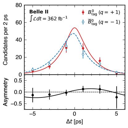
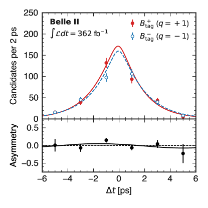
Figure 3: Distributions, and fit projections, of $\Delta t$ for flavor-tagged (left) $B^{0}\rightarrow\phi K^{0}_{S}$ and (right) $B^{+}\rightarrow\phi K^{+}$ candidates subtracted of the continuum background. The fit PDFs corresponding to $q=-1$ and $q=+1$ tagged distributions are shown as dashed and solid curves, respectively. The yield asymmetries, defined as $(N(q=+1)-N(q=-1))/(N(q=+1)+N(q=-1))$, are displayed in the bottom subpanels.

Table 1: Results of the fit to the signal and control samples.

	$B^{0}\rightarrow\phi K^{0}_{S}$	$B^{+}\rightarrow\phi K^{+}$
Resonant yield	$162\pm 17$	$581\pm 33$
Nonresonant yield	$21\pm 12$	$70\pm 23$
Continuum yield	$1169\pm 35$	$5730\pm 77$
$C$	$-0.31\pm 0.20$	$-0.12\pm 0.10$
$S$	$0.54\pm 0.26$	$-0.09\pm 0.12$

The fit results are reported in Table 1. In the control sample, we find $581\pm 33$ signal $B^{+}\rightarrow\phi K^{+}$, $70\pm 23$ nonresonant, and $5730\pm 77$ continuum events. The relevant data distributions are displayed in Fig. 1, with fit projections overlaid, under selections in the analysis variables that enhance the signal component. The control-sample $C\!P$ asymmetries are $\comment{C}=\comment{-0.12\pm 0.10}$ and $S=-0.09\pm 0.12$, where the uncertainties are statistical only, with correlation coefficient $\rho=\comment{0.06}$. The results are compatible with the null asymmetries we expect. In the fit to the signal $B^{0}\rightarrow\phi K^{0}_{S}$ sample, displayed under the same signal-enhancing selections in Fig. 2, we find $162\pm 17$ signal, $21\pm 12$ nonresonant, and $1169\pm 35$ continuum events. The corresponding $C\!P$ asymmetries are $\comment{C}=\comment{-0.31\pm 0.20}$ and $S=0.54\pm 0.26$, where the uncertainties are statistical only, with correlation coefficient $\rho=\comment{0.01}$. The observed continuum background asymmetry is compatible with zero. The $\Delta t$ distributions for tagged signal decays, after subtracting the continuum background Pivk and Le Diberder (2005), are displayed in Fig. 3, along with the resulting $C\!P$-violating asymmetries.

V Systematic uncertainties

Contributions from all considered sources of systematic uncertainty are listed in Table 2. We consider uncertainties associated with the calibration of the flavor tagging and resolution function, fit model, and determination of $\Delta t$.

The leading contribution to the total systematic uncertainty on $C$ arises by neglecting a possible time-integrated $C\!P$ asymmetry from $B\kern 1.79993pt\overline{\kern-1.79993ptB}{}$ backgrounds. The main systematic uncertainty on $S$ comes from the fit bias, due to the modest statistical precision to which the fraction of $B^{0}\rightarrow K^{+}K^{-}K^{0}_{S}$ backgrounds can be determined with the current sample size.

V.1 Calibration with $B^{0}\rightarrow D^{(*)-}\pi^{+}$ decays

We assess the uncertainty associated with the resolution function and flavor tagging parameters using simplified simulated samples. We generate ensembles assuming for each an alternative value for the above parameters sampled from the statistical covariance matrix determined in the $B^{0}\rightarrow D^{(*)-}\pi^{+}$ control sample. Each ensemble is fitted using the nominal values of the calibration parameters and the standard deviation of the observed biases is used as a systematic uncertainty.

A similar procedure is used to assess a systematic uncertainty due to the systematic uncertainties on the calibration parameters, in which the ensembles are generated by varying each parameter independently within their systematic uncertainty.

We estimate the impact of differences in the resolution function and tagging performance between the signal and calibration samples. We apply the resolution function and flavor-tagging calibration obtained from a simulated $B^{0}\rightarrow D^{(*)-}\pi^{+}$ sample and repeat the measurement of $C$ and $S$ over an ensemble of simulated $B^{0}\rightarrow\phi K^{0}_{S}$ events. The average deviation of the $C\!P$ asymmetries from their generated values is assigned as a systematic uncertainty.

V.2 Fit model

To validate how accurately the fit determines the underlying physics parameters in the presence of backgrounds, we generate ensemble datasets that contain all the fit components. For each ensemble, we sample alternative values of $C$ and $S$ within the physical boundaries, and the fraction of the resonant events over the sum of resonant and nonresonant decays between 0.7 and 1.0, to account for the statistical precision on the observed value $f_{\phi K}=0.89\pm 0.07$. Due to the limited sample size, we assign a conservative systematic uncertainty for the fit bias by taking the largest deviations of the fitted values of $C$ and $S$ from their generated values. We also check that the relative magnitude of this systematic uncertainty with respect to the statistical uncertainty remains constant for larger sample sizes.

We study the effect of neglecting interference between the signal and nonresonant backgrounds using simulated samples, where the $B^{0}\rightarrow\phi K^{0}_{S}$ and $B^{0}\rightarrow K^{+}K^{-}K^{0}_{S}$ components are generated coherently using a complete Dalitz-plot description of the decay Nakahama et al. (2010). We apply the nominal fit to these samples, where the nonresonant yields are determined by the fit and the $C\!P$-asymmetries of the backgrounds, $C_{K^{+}K^{-}K^{0}_{S}}$ and $S_{K^{+}K^{-}K^{0}_{S}}$, are fixed to their generated values, neglecting interference with the signal. The difference between the generated and fitted values of the $C\!P$-asymmetries of the signal is assigned as a systematic uncertainty.

The effect of fixing the PDF shapes of the $M_{\text{bc}}$, $\mathcal{O}^{{}^{\prime}}_{\text{CS}}$, $\cos\theta_{H}$, and $\Delta t$ distributions in continuum, and $\mathcal{O}^{{}^{\prime}}_{\text{CS}}$ distribution in signal and nonresonant background, is estimated from ensemble datasets. We generate simulated datasets by varying the shape parameters, in order to cover for the empirical parametrization and statistical uncertainty, and fix them to their nominal values in the fit. The resulting standard deviation on the distributions of $C$ and $S$ is used to estimate the corresponding systematic uncertainty.

The same procedure is applied to estimate the systematic uncertainty associated with the external inputs used for the lifetime $\tau_{B^{0}}=(1.519\pm 0.004)\leavevmode\nobreak\ {\rm\,ps}$, mixing frequency $\Delta m_{d}=(0.507\pm 0.002)\leavevmode\nobreak\ {\rm\,ps^{-1}}$, and $C\!P$ asymmetries $\comment{C}=0.06\pm 0.08$ and $S=-0.68^{+0.09}_{-0.10}$ of the nonresonant background.

Simulation shows that the residual $B\kern 1.79993pt\overline{\kern-1.79993ptB}{}$ backgrounds is at most 2% of the signal yield. We generate ensemble datasets containing an additional $B\kern 1.79993pt\overline{\kern-1.79993ptB}{}$ background component with PDF shapes modeled after the $B^{0}\rightarrow\phi K^{0}_{S}$ or $B^{0}\rightarrow K^{+}K^{-}K^{0}_{S}$ distributions and by conservatively varying the $B\kern 1.79993pt\overline{\kern-1.79993ptB}{}$ background $C\!P$ asymmetries between $+1$ and $-1$. The $B\kern 1.79993pt\overline{\kern-1.79993ptB}{}$ backgrounds are neglected in the fit to these datasets. The corresponding systematic uncertainty is obtained by taking the largest deviations of $C$ and $S$ from their generated values.

The time evolution given in Eq. (1) assumes that the $B_{\text{tag}}$ decays in a flavor-specific final state. We study the impact of the tag-side interference, i.e., neglecting the effect of CKM-suppressed $b\rightarrow u\overline{}cd$ decays in the $B_{\text{tag}}$ in the model for $\Delta t$ Long et al. (2003). The observed asymmetries can be corrected for this effect by using the knowledge from previous measurements Amhis et al. (2023). We conservatively assume all events to be tagged by hadronic $B$ decays, for which the effect is largest, and take the difference with respect to the observed asymmetries as a systematic uncertainty.

The effect of multiple candidates is evaluated by repeating the analysis with all the candidates and taking the difference with respect to the nominal candidate selection as a systematic uncertainty.

Table 2: Summary of systematic uncertainties.

Source	$\sigma(\comment{C})$	$\sigma(S)$
Calibration with $B^{0}\rightarrow D^{(*)-}\pi^{+}$ decays
Calibration sample size	$\pm 0.010$	$\pm 0.009$
Calibration sample systematic	$\pm 0.010$	$\pm 0.012$
Sample dependence	$+0.005$	$+0.021$
Fit model
Fit bias	${}^{\mbox{\footnotesize$+0.028$}}_{\mbox{\footnotesize$-0.017$}}$	${}^{\mbox{\footnotesize$+0.033$}}_{\mbox{\footnotesize$-0.062$}}$
$B^{0}\rightarrow K^{+}K^{-}K^{0}_{S}$ backgrounds	$+0.020$	$-0.011$
Fixed fit shapes	$\pm 0.009$	$\pm 0.022$
$\tau_{B^{0}}$ and $\Delta m_{d}$ uncertainties	$\pm 0.006$	$\pm 0.022$
$C_{K^{+}K^{-}K^{0}_{S}}$ and $S_{K^{+}K^{-}K^{0}_{S}}$	$\pm 0.014$	$\pm 0.013$
$B\overline{B}$ backgrounds	${}^{\mbox{\footnotesize$+0.019$}}_{\mbox{\footnotesize$-0.030$}}$	${}^{\mbox{\footnotesize$+0.017$}}_{\mbox{\footnotesize$-0.031$}}$
Tag-side interference	$<0.001$	$+0.012$
Multiple candidates	$-0.032$	$-0.002$
$\Delta t$ measurement
Detector misalignment	$-0.002$	$-0.002$
Momentum scale	$\pm 0.001$	$\pm 0.001$
Beam spot	$\pm 0.002$	$\pm 0.002$
$\Delta t$ approximation	$<0.001$	$-0.018$
Total systematic	${}^{\mbox{\footnotesize$+0.046$}}_{\mbox{\footnotesize$-0.052$}}$	${}^{\mbox{\footnotesize$+0.058$}}_{\mbox{\footnotesize$-0.082$}}$
Statistical	$\pm 0.201$	$\pm 0.256$

V.3 $\Delta t$ measurement

The impact of the detector misalignment is tested on simulated samples reconstructed with various misalignment configurations.

The uncertainty on the momentum scale of charged particles due to the imperfect modeling of the magnetic field has a small impact on the $C\!P$ asymmetries Adachi et al. .

Similarly, the uncertainty on the coordinates of the $e^{+}e^{-}$ interaction region (beam spot) has a subleading effect Adachi et al. .

We do not account for the angular distribution of the $B$ meson pairs in the c.m. frame when calculating $\Delta t$ using Eq. (2). Therefore, we estimate the effect of the $\Delta t$ approximation on simulated samples, where the generated and reconstructed time differences can be compared.

VI Summary

A measurement of $C\!P$ violation in $B^{0}\rightarrow\phi K^{0}_{S}$ decays is presented using data from the Belle II experiment. We find $162\pm 17$ signal candidates in a sample containing $(387\pm 6)\times 10^{6}$ $B\kern 1.79993pt\overline{\kern-1.79993ptB}{}$ events. The values of the $C\!P$ asymmetries are

$$\comment{C}=\comment{-0.31\pm 0.20\pm 0.05}\quad\text{and}\quad S=0.54\pm 0.26^{+0.06}_{-0.08},$$

where the first uncertainty is statistical, and the second is systematic. The results are compatible with previous determinations from Belle and BABAR Nakahama et al. (2010); Lees et al. (2012) and have a similar uncertainty on $C$, despite using a data sample $2.0$ and $1.2$ times smaller, respectively. When compared to measurements using a similar quasi-two-body approach Aubert et al. (2005); Chen et al. (2007), there is a 10% to 20% improvement on the statistical uncertainty on $S$ for the same number of signal events. No significant discrepancy in the $C\!P$ asymmetries between $b\rightarrow q\overline{}qs$ and $b\rightarrow c\overline{}cs$ transitions is observed.

References

- Cabibbo (1963) N. Cabibbo, Phys. Rev. Lett. 10, 531 (1963).
- Kobayashi and Maskawa (1973) M. Kobayashi and T. Maskawa, Prog. Theor. Phys. 49, 652 (1973).
- Amhis et al. (2023) Y. S. Amhis et al. (HFLAV Collaboration), Phys. Rev. D 107, 052008 (2023).
- Beneke (2005) M. Beneke, Phys. Lett. B 620, 143 (2005).
- (5) The coefficients (,) are written (, ) elsewhere.
- Workman et al. (2022) R. L. Workman et al. (Particle Data Group), Prog. Theor. Exp. Phys. 2022, 083C01 (2022).
- Abudinén et al. (2022) F. Abudinén et al. (Belle II Collaboration), Eur. Phys. J. C 82, 283 (2022).
- Nakahama et al. (2010) Y. Nakahama et al. (Belle Collaboration), Phys. Rev. D 82, 073011 (2010).
- Lees et al. (2012) J. P. Lees et al. (BABAR Collaboration), Phys. Rev. D 85, 112010 (2012).
- (10) T. Abe et al. (Belle II Collaboration), arXiv:1011.0352 .
- Adamczyk et al. (2022) K. Adamczyk et al. (Belle II SVD Collaboration), J. Instrum. 17, P11042 (2022).
- Jadach et al. (2000) S. Jadach, B. F. L. Ward, and Z. Wa̧s, Comput. Phys. Commun. 130, 260 (2000).
- Sjöstrand et al. (2015) T. Sjöstrand et al., Comput. Phys. Commun. 191, 159 (2015).
- Lange (2001) D. J. Lange, Nucl. Instrum. Methods Phys. Res., Sect A 462, 152 (2001).
- Agostinelli et al. (2003) S. Agostinelli et al. (GEANT4 Collaboration), Nucl. Instrum. Methods Phys. Res., Sect. A 506, 250 (2003).
- Kuhr et al. (2019) T. Kuhr, C. Pulvermacher, M. Ritter, T. Hauth, and N. Braun (Belle II Framework Software Group), Comput. Software Big Sci. 3, 1 (2019).
- (17) https://doi.org/10.5281/zenodo.5574115.
- Bertacchi et al. (2021) V. Bertacchi et al. (Belle II Tracking Group), Comput. Phys. Commun. 259, 107610 (2021).
- Hulsbergen (2005) W. D. Hulsbergen, Nucl. Instrum. Methods 552, 566 (2005).
- Krohn et al. (2020) J.-F. Krohn et al. (Belle II Analysis Software Group), Nucl. Instrum. Methods Phys. Res., Sect. A 976, 164269 (2020).
- Waltenberger et al. (2008) W. Waltenberger, W. Mitaroff, F. Moser, B. Pflugfelder, and H. V. Riedel, J. Phys. Conf. Ser. 119, 032037 (2008).
- Dey and Soffer (2020) S. Dey and A. Soffer, Springer Proc. Phys. 248, 411 (2020).
- Chen and Guestrin (2016) T. Chen and C. Guestrin, Proceedings of the 22nd ACM SIGKDD International Conference on Knowledge Discovery and Data Mining, (2016).
- Ed. A. J. Bevan, B. Golob, Th. Mannel, S. Prell, and B. D. Yabsley (2014) Ed. A. J. Bevan, B. Golob, Th. Mannel, S. Prell, and B. D. Yabsley, Eur. Phys. J. C 74, 3026 (2014).
- Lee et al. (2003) S. H. Lee et al. (Belle Collaboration), Phys. Rev. Lett. 91, 261801 (2003).
- Brandt et al. (1964) S. Brandt, C. Peyrou, R. Sosnowski, and A. Wroblewski, Phys. Lett. 12, 57 (1964).
- Farhi (1977) E. Farhi, Phys. Rev. Lett. 39, 1587 (1977).
- Fox and Wolfram (1978) G. C. Fox and S. Wolfram, Phys. Rev. Lett. 41, 1581 (1978).
- Albrecht et al. (1990) H. Albrecht et al. (ARGUS Collaboration), Phys. Lett. B 241, 278 (1990).
- Abudinén et al. (2023) F. Abudinén et al. (Belle II Collaboration), Phys. Rev. D 107, L091102 (2023).
- (31) I. Adachi et al. (Belle II Collaboration), arXiv:2302.12898 .
- Pivk and Le Diberder (2005) M. Pivk and F. R. Le Diberder, Nucl. Instrum. Methods Phys. Res., Sect. A 555, 356 (2005).
- Long et al. (2003) O. Long, M. Baak, R. N. Cahn, and D. Kirkby, Phys. Rev. D 68, 034010 (2003).
- Aubert et al. (2005) B. Aubert et al. (BABAR Collaboration), Phys. Rev. D 71, 091102 (2005).
- Chen et al. (2007) K.-F. Chen et al. (Belle Collaboration), Phys. Rev. Lett. 98, 031802 (2007).