Sensor Allocation and Online-Learning-based Path Planning for Maritime Situational Awareness Enhancement: A Multi-Agent Approach

Abstract

Countries with access to large bodies of water often aim to protect their maritime transport by employing maritime surveillance systems. However, the number of available sensors (e.g., cameras) is typically small compared to the to-be-monitored targets, and their Field of View (FOV) and range are often limited. This makes improving the situational awareness of maritime transports challenging. To this end, we propose a method that not only distributes multiple sensors but also plans paths for them to observe multiple targets, while minimizing the time needed to achieve situational awareness. In particular, we provide a formulation of this sensor allocation and path planning problem which considers the partial awareness of the targets' state, as well as the unawareness of the targets' trajectories. To solve the problem we present two algorithms: 1) a greedy algorithm for assigning sensors to targets, and 2) a distributed multi-agent path planning algorithm based on regret-matching learning. Because a quick convergence is a requirement for algorithms developed for high mobility environments, we employ a forgetting factor to quickly converge to correlated equilibrium solutions. Experimental results show that our combined approach achieves situational awareness more quickly than related work.

I Introduction

In Australia, 99% of all exports rely on maritime transport; in recognition of this, the Departure of Home Affairs has recently commenced the Future Maritime Surveillance Capability project [1]. One of those project aims is to reduce current and emerging threats to Australian maritime transport. According to [2], threats include unauthorized maritime arrivals, maritime terrorism, and piracy, robbery or violence at sea.

In addition to governmental institutions, researchers have also increasingly been paying attention to the ocean [3, 4]. In particular, achieving maritime situational awareness is an important task for researchers when they are designing maritime surveillance systems. Such systems need to deal with complex and time-varying environments. Specifically, targets, such as fishing boats or sailing boats, can frequently change their directions, and their long-term trajectories are typically unknown. In addition, the number of available sensors, e.g., cameras, may be quite low (compared to the number of vessels present in commercial straits or harbours) while detecting range and FOV of cameras are limited. As a result, resource allocation and sensor path-planning in real time are essential to address these issues [5, 6, 7].

In this paper, we consider scenarios where targets can initially be outside the coverage range of some sensors. Moreover, our sensors are cameras, radars and automatic identification systems (AIS). However, unlike [8] and [9], we place these cameras onboard of boats, e.g. guard boats, or unmanned surface vehicles (USVs). Thus, the sensors can move forward towards their targets in order to capture images and videos of these targets. Here, we assume that both the sensors and their targets move across the surface of a sea.

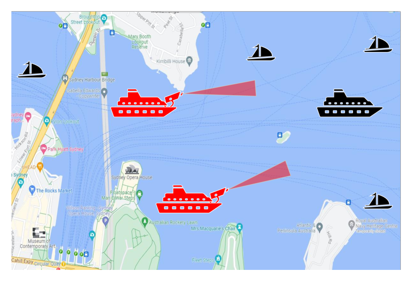
Figure 1: An illustration of Sydney Harbor [10]. In this scenario, 1) the two red boats are guard boats equipped with camera whose horizontal FOV is $3\degree$, and 2) black vessels are targets which the two guard boats attempt to observe. Vessels and cameras are not drawn to scale.

We define by $\mathcal{C}$ and $\mathcal{V}$ a set of available cameras used and a set of targets, respectively. Thus, $|\mathcal{C}|$ is the number of cameras while $|\mathcal{V}|$ is the number of targets. Each target $v\in\mathcal{V}$ moves around in the area that is to be monitored, e.g., Sydney Harbor in Australia (see Fig. 1), and the target may initially not reside within the sensing range of any camera $c\in\mathcal{C}$. Here, the cameras are not only partially aware of targets' states, but they are also unaware of target trajectories. Thus, we need to estimate the targets' locations over a time horizon. First, we assume that the motion of $|\mathcal{V}|$ targets is linear without any changes in moving speeds or directions. This assumption is reasonable because ships typically travel along sea lanes in harbors according to maritime vessel traffic [11]. Then, we rely on this assumption and our measurements that are collected by a stationary radar $r$ and the AIS to estimate future positions of targets.

In practice, radars and cameras can determine the range and bearing on their own , while AIS broadcast information about location and speed of vessels [9]. Like [12, 13, 14], we assume that the radar, AIS and cameras provide us with observations of the targets' location. Then, we estimate the targets' location using Kalman filters and probabilistic data association. Cameras in the set $\mathcal{C}$ will use the estimate to independently plan a path to move forward until the targets are inside their FOV. Here, they generate their own paths by picking a moving angle and a speed from a finite set of angles and a finite set of speed levels, respectively. In addition, we have to allocate the cameras to the targets and plan the cameras' trajectories. Here, we are partially aware of target state through measurements from the radar and AIS while the target trajectories are unknown. It makes both allocating limited resources and planning cameras' trajectories challenging.

I-A Background

Due to uncertainties in high mobility environments like maritime situations [15, 16, 17, 18], a number of research projects focus on maximizing sensors' coverage area or on planning paths for sensors to accurately sense targets. Specifically, [19] attempts to maximize sensor coverage in wireless sensor networks (WSN) using a local search-based algorithm. In addition, the authors mathematically determine the upper and lower bounds of coverage deployment. Compared to [19], who minimize the WSN cost, [20] uses a meta-heuristic algorithm to optimize the number of sensors and their locations. In contrast to these works, [21] considers uncertainties of response time and demand in the problem of locating emergency service facilities. Relying on an uncertainty theory, the authors model the maximal location problem under the uncertainties; then, they transform the model into an equivalent deterministic problem to solve it. However, all these works require knowledge of the target trajectories.

To track targets moving with an unknown trajectory, [22, 23, 24, 25, 26, 27, 28, 29, 30, 31] estimate targets' position and velocity, and then determine trajectory for USVs, autonomous underwater vehicles (AUVs) or UAVs. For example, [22, 23, 24] propose algorithms to track the trajectory of a single USV under unknown system dynamics. Based on range measurement, [25] predicts a target's future position based on its past trajectory and estimated velocity. Then, a reference path that closely follows the target's predicted path is generated. A controller uses feedback from the AUV's sensors to follow the reference path while maintaining a safe distance from the target. Similarly, [26] and [29] employ data collection, target analysis, resource optimization or route optimization, while their goal is to improve the accuracy and effectiveness in tracking multiple targets. Interestingly, the work of [26] is effective only when sensors are stationary and when targets always stay inside the sensors' sensing range. As another limitation, [29] demonstrate a resource management scheme in the scenario where only one mobile sensor is employed.

To plan paths for multiple mobile sensors or UAVs, [13, 32, 33, 34] propose algorithms based on the partially observable Markov decision process (POMDP) framework [35]. In [13], UAVs are guided to track multiple ground targets by selecting the best velocity and heading angle for the UAVs. That work also takes the effects of wind into account when controlling UAVs. Instead of designing a path-planning algorithm, [34] focuses on determining the positions of UAVs in the future with the target which is to search and track multiple mobile objects. Both [13] and [34] do not resolve the issue where the targets do not traverse within the coverage range of the sensors initially. Unlike [13, 34], the work of [36] introduces an algorithm which plans for multiple sensors to follow multiple targets leaving the sensors’ observation range.

One significant issue with the algorithms in [13, 34, 36] is that they are only efficient (or demonstrated) in scenarios where the number of sensors and targets is limited to three and five, respectively. Additionally, these algorithms may not converge to an optimal solution. To tackle this issue, [37] and [38] have utilized regret-matching learning, a form of online learning, to create multi-agent system algorithms whose convergence is guaranteed. According to [39], regret-matching learning is a strategy designed for agents to learn how to make decisions over time. Specifically, each agent will play an action with respect to its probability, which is proportional to the gain of that action, and the action gain is measured by regrets. The effectiveness of regret-matching learning-based algorithms is shown in various applications such as seasonal forecasting and matching markets without incentives [40, 41, 42, 43]. Additionally, the regret-matching learning-based algorithms in [44] and [45], have been shown to converge to correlated-equilibrium solutions more quickly than reinforcement-learning-based algorithms. However, these existing works [37, 38, 40, 41, 42, 43, 44, 45] have not considered any problems related to allocation and planning.

I-B Contribution

In this paper, we propose a multi-sensor allocation and planning approach to observe multiple targets with unknown trajectories, while minimizing the time required to achieve situational awareness. Unlike [13, 34, 36], we consider that the number of available mobile cameras can be large, e.g., 30 cameras, and that it is lower than the number of targets. The targets are (at times) outside the limited FOV of cameras. Due to the partial awareness of target state, as well as the unawareness of target trajectory in the next time, planning multiple cameras' paths to observe all multiple targets during a short time in this scenario is a non-trivial problem. To solve this problem, we will assign cameras to targets; these cameras then make their own plan to move forward to the targets using regret-matching learning. We summarize the contributions of this paper in the following.

1. Unlike [13], we formulate a problem to not only assign cameras to targets but to also generate a trajectory for each camera over a time horizon for the given maritime situation. In particular, the partial awareness of target state, and the unawareness of target trajectory are taken into account in our problem formulation.

2. Due to the complexity and the large size of our formulated problem, i.e., a large number of sensors and targets, or a long time horizon, we propose two algorithms: a sensor allocation algorithm and a distributed multi-agent path planning algorithm, to deal with the problem. Using the sensor-target distance and the duration that a target has not been observed, the former allocates cameras to targets to shorten the duration of observing all the targets. Subsequently, the latter employs regret-matching learning so that the sensors create their trajectory as individual agents in a multi-agent system. In our online-learning process, we use a forgetting factor to make the proposed distributed algorithm converge quickly to a correlated equilibrium, similar to our previous work [46].

3. We evaluate the performance using computational experiments that extend scenarios from the literature by several orders of magnitude. The results demonstrate the efficiency of our proposed approach to achieve situational awareness, especially in scenarios involving many cameras and targets.

The remainder of the paper is organized as follows. Section II presents the system model, including a dynamic model and a measurement model, while Section III describes the problem formulation for sensor allocation and path planning over a time horizon. Then, we describe in Section IV our multi-sensor allocation algorithm and our distributed multi-agent path planning algorithm. Section V reports on our experiments to illustrate the efficiency of the proposed approach. Finally, we summarize the paper in Section VI.

II System Model

To formulate the problem, we need to model the mobility of targets, as well as the observations (measurements) of radars, AIS and cameras. The models of target motion and sensor measurement are described in the following subsections.

II-A Dynamic Model

Like [9], we assume that each target in our maritime scenario follows a nearly-constant velocity (NCV) model. The NCV model is given by:

$$\mathbb{x}^{v}_{t+1} =\mathbb{F}_{t}\cdot\mathbb{x}^{v}_{t}+\mathbb{w}^{v}_{t}$$ (1)

with

$$\mathbb{x}^{v}_{t} =(x^{v}_{t}\quad\dot{x}^{v}_{t}\quad y^{v}_{t}\quad\dot{y}^{v}_{t})^{T},$$ (2)

$$\mathbb{F}_{t} =\begin{pmatrix}1&\Delta t&0&0\\ 0&1&0&0\\ 0&0&1&\Delta t\\ 0&0&0&1\end{pmatrix},$$

where $x^{v}_{t}$ and $y^{v}_{t}$ are target $v$'s position while $\dot{x}^{v}_{t}$ and $\dot{y}^{v}_{t}$ are target $v$'s velocity at time step $t$ in a 2-D coordinate system. $\mathbb{x}^{T}$ is the transposition of vector $\mathbb{x}$. In addition, $\Delta{t}$ is the duration of each time step while $\mathbb{F}_{t}$ is a motion model for all targets. $\mathbb{w}^{v}_{t}\sim N(0,\mathbb{Q}^{v}_{t})$ is zero-mean white Gaussian process noise with the following covariance $\mathbb{Q}^{v}_{t}$.

$$\mathbb{Q}^{v}_{t} ={\sigma_{v}}^{2}\begin{bmatrix}\frac{(\Delta t)^{3}}{3}&\frac{(\Delta t)^{2}}{2}&0&0\\ \frac{(\Delta t)^{2}}{2}&\frac{(\Delta t)^{3}}{3}&0&0\\ 0&0&\frac{(\Delta t)^{3}}{3}&\frac{(\Delta t)^{2}}{2}\\ 0&0&\frac{(\Delta t)^{2}}{2}&\frac{(\Delta t)^{3}}{3}\end{bmatrix}.$$ (3)

II-B Measurement Model

Like [13, 36], we model the observations of the radar $r$, AIS and each camera $c\in\mathcal{C}$, respectively, in the following.

$$\mathbb{z}^{rv}_{t}\quad =\quad\mathbb{H}^{r}_{t}\cdot\mathbb{x}^{v}_{t}+\mathbb{v}^{rv}_{t}$$ (4)

$$\mathbb{z}^{\text{AIS}v}_{t}\quad =\quad\mathbb{H}^{\text{AIS}}_{t}\cdot\mathbb{x}^{v}_{t}+\mathbb{v}^{\text{AIS}}_{t}$$

$$\mathbb{z}^{cv}_{t}\quad =\quad\mathbb{H}^{c}_{t}\cdot\mathbb{x}^{v}_{t}+\mathbb{v}^{cv}_{t}$$

with

$$\mathbb{H}^{r}_{t}=\mathbb{H}^{\text{AIS}}_{t}=\mathbb{H}^{c}_{t} =\begin{pmatrix}1&0&0&0\\ 0&0&1&0\end{pmatrix},$$ (5)

where $\mathbb{H}^{r}_{t}$, $\mathbb{H}^{\text{AIS}}_{t}$ and $\mathbb{H}^{c}_{t}$ are the observation models of radar $r$, AIS and camera $c$, respectively. Moreover, $\mathbb{v}^{rv}_{t}\sim N(0,\mathbb{R}^{rv}_{t})$, $\mathbb{v}^{\text{AIS}}_{t}\sim N(0,\mathbb{R}^{\text{AIS}}_{t})$ and $\mathbb{v}^{cv}_{t}\sim N(0,\mathbb{R}^{cv}_{t})$ are additive noise terms. Then, $\mathbb{R}^{rv}_{t}$, $\mathbb{R}^{\text{AIS}}_{t}$ and $\mathbb{R}^{cv}_{t}$ are determined as follows:

$$\mathbb{R}^{rv}_{t} =\quad{{\sigma}^{rv}_{t}}^{2}\begin{pmatrix}1&0\\ 0&1\end{pmatrix}$$ (6)

$$\mathbb{R}^{\text{AIS}}_{t} =\quad{{\sigma}^{\text{AIS}}}^{2}\begin{pmatrix}1&0\\ 0&1\end{pmatrix}$$

$$\mathbb{R}^{cv}_{t} =\quad{{\sigma}^{cv}_{t}}^{2}\begin{pmatrix}1&0\\ 0&1\end{pmatrix}.$$

In a maritime environment, only uncertainties in the observations of radars and cameras depend on the distance between these observers and their targets. Thus, in Eq. (6), ${\sigma^{rv}_{t}}$ and ${\sigma^{cv}_{t}}$ are positive proportional to the distance from radar $r$ or camera $c$ to target $v$ at time step $t$ while ${\sigma^{\text{AIS}}}$ is assumed to be constant (because it is GPS-based).

III Problem Formulation

To assign targets to cameras and to plan trajectories for these cameras (possibly over a long time horizon), we have to estimate the targets' positions using the observations collected by radar $r$, AIS and cameras. Furthermore, in this paper, we consider that the overall maritime situational awareness is achieved (albeit temporarily) once all targets are observed at least once. Here, we define that a target is observed by a camera if it resides within the camera' detection range and FOV, and the mean squared error (MSE) between its estimated value and ground truth is equal to or less than a pre-given threshold.

In this paper, a target $v$ can be observed by radar $r$, AIS and camera $c$; thus, by building on [13], the total MSE of $|\mathcal{V}|$ targets is calculated over a time horizon $H$ as follows:

$$J_{H} \approx\sum_{t=\tilde{t}+0}^{\tilde{t}+H-1}\sum_{v\in\mathcal{V}}\text{Tr}\left(\tilde{\mathbb{P}}^{v}_{t+1}\right)$$ (7)

$$=\sum_{t=\tilde{t}+0}^{\tilde{t}+H-1}\sum_{v\in\mathcal{V}}\text{Tr}\left(\frac{1}{\frac{1}{\tilde{\mathbb{P}}^{rv}_{t+1}}+\frac{1}{\tilde{\mathbb{P}}^{\text{AIS}v}_{t+1}}+\frac{1}{\tilde{\mathbb{P}}^{cv}_{t+1}}}\right),$$

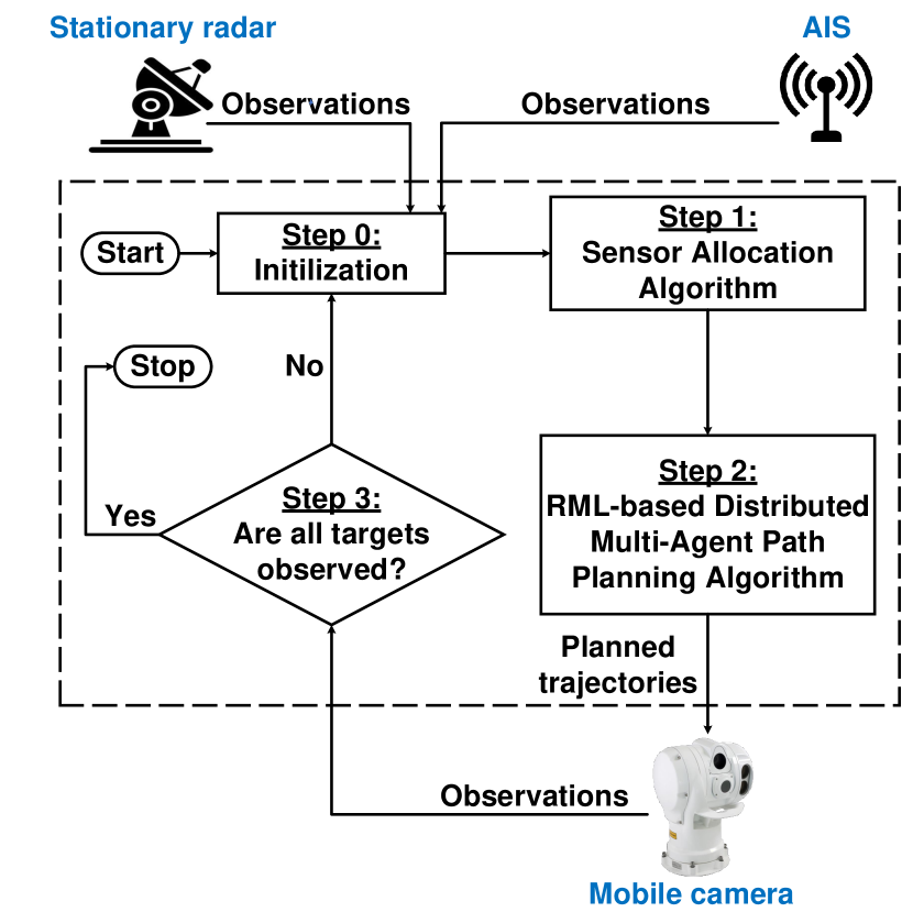
Figure 2: Flowchart of the proposed Sensor Allocation and Path Planning approach.

where $t=\tilde{t}+0$ is the current time step; and $\text{Tr}\left(\tilde{\mathbb{P}}^{v}_{t+1}\right)$ is the trace of matrix $\tilde{\mathbb{P}}^{v}_{t+1}$. Here, $\tilde{\mathbb{P}}^{v}_{t+1}$ is the covariance update of target $v$ at time step $t+1$. To compute $\tilde{\mathbb{P}}^{rv}_{t+1}$, $\tilde{\mathbb{P}}^{\text{AIS}v}_{t+1}$ and $\tilde{\mathbb{P}}^{cv}_{t+1}$, we have

$$\tilde{\mathbb{P}}^{rv}_{t+1}=\begin{cases}\frac{1}{\frac{1}{\tilde{\mathbb{P}}^{rv}_{t+1|t}}+\mathbb{S}^{rv}_{t+1}}&\text{if $v$ is observed by $r$},\\ \tilde{\text{P}}^{rv}_{t+1|t}&\text{otherwise}\end{cases}$$ (8)

$$\tilde{\mathbb{P}}^{\text{AIS}v}_{t+1}=\begin{cases}\frac{1}{\frac{1}{\tilde{\mathbb{P}}^{\text{AIS}v}_{t+1|t}}+\mathbb{S}^{\text{AIS}v}_{t+1}}&\text{if $v$ is observed by AIS},\\ \tilde{\mathbb{P}}^{\text{AIS}v}_{t+1|t}&\text{otherwise}\end{cases}$$

$$\tilde{\mathbb{P}}^{cv}_{t+1}=\begin{cases}\frac{1}{\frac{1}{\tilde{\mathbb{P}}^{cv}_{t+1|t}}+\mathbb{S}^{cv}_{t+1}}&\text{if $v$ is observed by $c$},\\ \tilde{\mathbb{P}}^{cv}_{t+1|t}&\text{otherwise}\end{cases},$$

where $\tilde{\mathbb{P}}^{rv}_{t+1|t}=\mathbb{F}_{t}\cdot\tilde{\mathbb{P}}^{rv}_{t}\cdot\mathbb{F}^{T}_{t}+\mathbb{Q}^{v}_{t}$, $\tilde{\mathbb{P}}^{\text{AIS}v}_{t+1|t}=\mathbb{F}_{t}\cdot\tilde{\mathbb{P}}^{\text{AIS}v}_{t}\cdot\mathbb{F}^{T}_{t}+\mathbb{Q}^{v}_{t}$ and $\tilde{\mathbb{P}}^{cv}_{t+1|t}=\mathbb{F}_{t}\cdot\tilde{\mathbb{P}}^{cv}_{t}\cdot\mathbb{F}^{T}_{t}+\mathbb{Q}^{v}_{t}$. Additionally, $\mathbb{S}^{rv}_{t+1}$, $\mathbb{S}^{\text{AIS}v}_{t+1}$ and $\mathbb{S}^{cv}_{t+1}$ are the measurement prediction covariance of radar $r$, AIS and camera $c$ when they observe target $v$. Then, we have $\mathbb{S}^{rv}_{t+1}={\mathbb{H}^{r}_{t+1}}^{T}\cdot\mathbb{R}^{rv}_{t+1}\cdot\mathbb{H}^{r}_{t+1}$, $\mathbb{S}^{\text{AIS}v}_{t+1}={\mathbb{H}^{\text{AIS}}_{t+1}}^{T}\cdot\mathbb{R}^{\text{AIS}}_{t+1}\cdot\mathbb{H}^{\text{AIS}}_{t+1}$ and $\mathbb{S}^{cv}_{t+1}={\mathbb{H}^{c}_{t+1}}^{T}\cdot\mathbb{R}^{cv}_{t+1}\cdot\mathbb{H}^{c}_{t+1}$. We assume that target $v$ will be observed by radar $r$, AIS and camera $c$ at time step $t+1$ if target $v$'s nominal mean positions defined by $\tilde{\xi}^{rv}_{t+1}$, $\tilde{\xi}^{\text{AIS}v}_{t+1}$ and $\tilde{\xi}^{cv}_{t+1}$ are in the coverage area of radar $r$ and AIS, and the FOV of camera $c$, respectively. Similar to [13], we calculate $\tilde{\xi}^{rv}_{t+1}$, $\tilde{\xi}^{\text{AIS}v}_{t+1}$ and $\tilde{\xi}^{cv}_{t+1}$, respectively, as follows:

$$\tilde{\xi}^{rv}_{t+1} =\quad\mathbb{F}_{t}\cdot\tilde{\xi}^{rv}_{t},$$ (9)

$$\tilde{\xi}^{\text{AIS}v}_{t+1} =\quad\mathbb{F}_{t}\cdot\tilde{\xi}^{\text{AIS}v}_{t},$$

$$\tilde{\xi}^{cv}_{t+1} =\quad\mathbb{F}_{t}\cdot\tilde{\xi}^{cv}_{t}.$$

When $t=\tilde{t}+0$, ($\tilde{\xi}^{rv}_{t}$, $\tilde{\mathbb{P}}^{rv}_{t}$), ($\tilde{\xi}^{\text{AIS}v}_{t}$,$\tilde{\mathbb{P}}^{\text{AIS}v}_{t}$) and ($\tilde{\xi}^{cv}_{t}$,$\tilde{\mathbb{P}}^{cv}_{t}$) are the state update and covariance update of target $v$ tracked by radar $r$, AIS and camera $c$, respectively. In addition, we calculate ($\tilde{\xi}^{rv}_{t}$, $\tilde{\mathbb{P}}^{rv}_{t}$), ($\tilde{\xi}^{\text{AIS}v}_{t}$,$\tilde{\mathbb{P}}^{\text{AIS}v}_{t}$) and ($\tilde{\xi}^{cv}_{t}$,$\tilde{\mathbb{P}}^{cv}_{t}$) using Kalman filter and probabilistic data association.

By using Eqs. (7), (8) and (9), we formulate the optimization problem of multi-sensor allocation and path planning over a time horizon $H$ in the following.

$$\min_{\hat{x}^{cv}_{t},s^{c}_{t},\phi^{c}_{t}}\quad\begin{split}&\sum_{t=\tilde{t}+0}^{\tilde{t}+H-1}\Bigg{\{}\sum_{v\in\mathcal{V}}\Big{[}\Big{(}\text{Tr}\left({\leavevmode\vbox{\offinterlineskip\hbox to0.0pt{\hbox to6.80557pt{\hss\vbox to2.52777pt{\hbox{\hbox{\char 3\relax}}\vss}\hss}\hss} \kern-0.86108pt\hbox{{\leavevmode\vbox{\offinterlineskip\hbox to0.0pt{\hbox to6.80557pt{\hss\vbox to2.52777pt{\hbox{\hbox{\char 3\relax}}\vss}\hss}\hss} \kern 0.0pt \hbox{{P}}}}}}}^{v}_{t+1}\right)-\epsilon\Big{)}\\ &+\alpha_{1}\sum_{c\in\mathcal{C}}\hat{x}^{cv}_{t}(D_{\min}-\tilde{d}^{cv}_{t+1})(\tilde{d}^{cv}_{t+1}-D_{\max})\\ &+\alpha_{2}\sum_{c\in\mathcal{C}}(D_{\text{safe}}-\tilde{d}^{cv}_{t+1})\Big{]}\\ &+\alpha_{3}\sum_{c\in\mathcal{C}}\sum_{c^{\prime}\in\mathcal{C},c^{\prime}\neq c}(D_{\text{safe}}-d^{cc^{\prime}}_{t+1})\Bigg{\}}\end{split}$$ (10a)

$$\text{s.t.}\quad\begin{split}&s_{\min}\leq s^{c}_{t}\leq s_{\max}\\ &\quad\quad\forall c\in\mathcal{C};t=\tilde{t}+0,\dots,\tilde{t}+H-1\end{split}$$ (10b)

$$\begin{split}&0\leq|\phi^{c}_{t}-\phi^{c}_{t-1}|\leq\Phi_{\max}\\ &\quad\quad\forall c\in\mathcal{C};t=\tilde{t}+0,\dots,\tilde{t}+H-1\end{split}$$ (10c)

$$\begin{split}&\sum_{c\in\mathcal{C}}x^{cv}_{t}\leq 1\\ &\quad\quad\forall v\in\mathcal{V};t=\tilde{t}+0,\dots,\tilde{t}+H-1\end{split}$$ (10d)

$$\begin{split}&\sum_{v\in\mathcal{V}}x^{cv}_{t}=1\\ &\quad\quad\forall c\in\mathcal{C};t=\tilde{t}+0,\dots,\tilde{t}+H-1\end{split}$$ (10e)

with

$${\leavevmode\vbox{\offinterlineskip\hbox to0.0pt{\hbox to6.80557pt{\hss\vbox to2.52777pt{\hbox{\hbox{\char 3\relax}}\vss}\hss}\hss} \kern-0.86108pt\hbox{{\leavevmode\vbox{\offinterlineskip\hbox to0.0pt{\hbox to6.80557pt{\hss\vbox to2.52777pt{\hbox{\hbox{\char 3\relax}}\vss}\hss}\hss} \kern 0.0pt \hbox{{P}}}}}}}^{v}_{t+1}=\frac{1}{\frac{1}{\tilde{\mathbf{P}}^{rv}_{t+1}}+\frac{1}{\tilde{\mathbf{P}}^{\text{AIS}v}_{t+1}}+\sum_{c\in\mathcal{C}}\frac{\hat{x}^{cv}_{t}}{\tilde{\mathbf{P}}^{cv}_{t+1}}},$$ (11)

where $\text{Tr}\left({\leavevmode\vbox{\offinterlineskip\hbox to0.0pt{\hbox to6.80557pt{\hss\vbox to2.52777pt{\hbox{\hbox{\char 3\relax}}\vss}\hss}\hss} \kern-0.86108pt\hbox{{\leavevmode\vbox{\offinterlineskip\hbox to0.0pt{\hbox to6.80557pt{\hss\vbox to2.52777pt{\hbox{\hbox{\char 3\relax}}\vss}\hss}\hss} \kern 0.0pt \hbox{{P}}}}}}}^{v}_{t+1}\right)$ is the trace of matrix ${\leavevmode\vbox{\offinterlineskip\hbox to0.0pt{\hbox to6.80557pt{\hss\vbox to2.52777pt{\hbox{\hbox{\char 3\relax}}\vss}\hss}\hss} \kern-0.86108pt\hbox{{\leavevmode\vbox{\offinterlineskip\hbox to0.0pt{\hbox to6.80557pt{\hss\vbox to2.52777pt{\hbox{\hbox{\char 3\relax}}\vss}\hss}\hss} \kern 0.0pt \hbox{{P}}}}}}}^{v}_{t+1}$; and $\epsilon$ is the MSE threshold. We use $\hat{x}^{cv}_{t}$ for assigning a target $v$ to a camera $c$. If $\hat{x}^{cv}_{t}=1$, target $v$ is assigned to camera $c$. Otherwise, target $v$ is not assigned to camera $c$. Moreover, $s^{c}_{t}$ and $\phi^{c}_{t}$ are speed and moving angle of camera $c$, respectively, at time step $t$. Different from [13, 47], the objective function in (10a) includes the following four terms: 1) MSE, 2) the distance between the position of camera $c$ and the nominal mean position of target $v$ assigned to $c$, 3) the distance between the nominal mean position of target $v$ and the position of all cameras, and 4) the distance between a camera and another cameras at time step $t+1$. Here, the second term is employed to maintain that camera $c$ has to move forward until its target $v$ resides within its FOV if $c$ wants to observe $v$. Then, because cameras and targets move on the same surface (the surface of a sea), we use the third and fourth terms to guarantee a safety distance between cameras and targets. In addition, we have

$$\text{Tr}\left({\leavevmode\vbox{\offinterlineskip\hbox to0.0pt{\hbox to6.80557pt{\hss\vbox to2.52777pt{\hbox{\hbox{\char 3\relax}}\vss}\hss}\hss} \kern-0.86108pt\hbox{{\leavevmode\vbox{\offinterlineskip\hbox to0.0pt{\hbox to6.80557pt{\hss\vbox to2.52777pt{\hbox{\hbox{\char 3\relax}}\vss}\hss}\hss} \kern 0.0pt \hbox{{P}}}}}}}^{v}_{t+1}\right)-\epsilon=\begin{cases}0&\text{if $\text{Tr}\left({\leavevmode\vbox{\offinterlineskip\hbox to0.0pt{\hbox to6.80557pt{\hss\vbox to2.52777pt{\hbox{\hbox{\char 3\relax}}\vss}\hss}\hss} \kern-0.86108pt\hbox{{\leavevmode\vbox{\offinterlineskip\hbox to0.0pt{\hbox to6.80557pt{\hss\vbox to2.52777pt{\hbox{\hbox{\char 3\relax}}\vss}\hss}\hss} \kern 0.0pt \hbox{{P}}}}}}}^{v}_{t+1}\right)\leq\epsilon$},\\ \text{Tr}\left({\leavevmode\vbox{\offinterlineskip\hbox to0.0pt{\hbox to6.80557pt{\hss\vbox to2.52777pt{\hbox{\hbox{\char 3\relax}}\vss}\hss}\hss} \kern-0.86108pt\hbox{{\leavevmode\vbox{\offinterlineskip\hbox to0.0pt{\hbox to6.80557pt{\hss\vbox to2.52777pt{\hbox{\hbox{\char 3\relax}}\vss}\hss}\hss} \kern 0.0pt \hbox{{P}}}}}}}^{v}_{t+1}\right)-\epsilon&\text{otherwise}\end{cases}$$ (12a)

$$D_{\min}-\tilde{d}^{cv}_{t+1}=\begin{cases}1&\text{if $\tilde{d}^{cv}_{t+1}\geq D_{\min}$},\\ D_{\min}-\tilde{d}^{cv}_{t+1}&\text{otherwise}\end{cases}$$ (12b)

$$\tilde{d}^{cv}_{t+1}-D_{\max}=\begin{cases}1&\text{if $\tilde{d}^{cv}_{t+1}\leq D_{\max}$},\\ \tilde{d}^{cv}_{t+1}-D_{\max}&\text{otherwise}\end{cases}$$ (12c)

$$D_{\text{safe}}-\tilde{d}^{cv}_{t+1}=\begin{cases}0&\text{if $\tilde{d}^{cv}_{t+1}\geq D_{\text{safe}}$},\\ D_{\text{safe}}-\tilde{d}^{cv}_{t+1}&\text{otherwise}\end{cases}$$ (12d)

$$D_{\text{safe}}-d^{cc^{\prime}}_{t+1}=\begin{cases}0&\text{if $d^{cc^{\prime}}_{t+1}\geq D_{\text{safe}}$},\\ D_{\text{safe}}-d^{cc^{\prime}}_{t+1}&\text{otherwise}\end{cases}$$ (12e)

where the values of $D_{\min}$, $D_{\max}$ and $D_{\text{safe}}$ are pre-given; and $\alpha_{1}$, $\alpha_{2}$ and $\alpha_{3}$ are scaling factors $(\alpha_{1},\alpha_{2},\alpha_{3}\in[0;1])$. Additionally, $\tilde{d}^{cv}_{t+1}$ is the distance between the position of camera $c$ and the nominal mean position $\tilde{\xi}^{cv}_{t+1}$ of target $v$ while $d^{cc^{\prime}}_{t+1}$ is the distance between camera $c$ and camera $c^{\prime}$ at time step $t+1$. Given $s^{c}_{t}$ and $\phi^{c}_{t}$, the position of camera $c$ at time step $t+1$ is determined using the following movement model, which is applicable to maritime situations [48].

$$\begin{cases}x^{c}_{t+1}=x^{c}_{t}+s^{c}_{t}\cdot\text{cos}(\phi^{c}_{t})\cdot\Delta t\\ y^{c}_{t+1}=y^{c}_{t}+s^{c}_{t}\cdot\text{sin}(\phi^{c}_{t})\cdot\Delta t\end{cases},$$ (13)

where $x^{c}_{t}$ and $y^{c}_{t}$ are positions of camera $c$ in a 2-D coordinate system (the sea surface) at time step $t$. Conditions (10b) and (10c) describe the range for speed and moving angle of each mobile camera $c$. Condition (10d) shows that one target must not be assigned to more than one camera at each time step because the number of cameras is inadequate. Moreover, condition (10e) defines that a camera only approaches a target until the target resides within the camera FOV. This constraint mimics human observer who focuses on one target at a time.

Algorithm 1 The proposed Sensor Allocation and RML-based distributed Path Planning approach

1: Input: A camera set $\mathcal{C}$, a target set $\mathcal{V}$, the current position of $\mathcal{C}$ cameras, and the information about $\mathcal{V}$ targets collected up to the current time step $t=\tilde{t}+0$;

2: Output: Camera-target allocation $\hat{x}^{cv}_{t}$, camera speed $s^{c}_{t}$, and camera moving angle $\phi^{c}_{t}$ ;

3: Step 0 (Initialization):

4:  Calculate nominal mean and covariance ($\tilde{\xi}^{rv}_{t}$,$\tilde{\mathbb{P}}^{rv}_{t}$), ($\tilde{\xi}^{\text{AIS}v}_{t}$,$\tilde{\mathbb{P}}^{\text{AIS}v}_{t}$) and    ($\tilde{\xi}^{cv}_{t}$,$\tilde{\mathbb{P}}^{cv}_{t}$) at the current time step $t=\tilde{t}+0$ using Kalman filter and    probabilistic data association;

5: Step 1 (Multi-Sensor Allocation Algorithm):

6:  for $t=\tilde{t}+0,\tilde{t}+1,\dots,\tilde{t}+H-1$

7:   If $t=\tilde{t}+0$

8:    Compute the allocation matrix $\mathbf{M}_{t}$ using Eqs. (14) and (15);

9:    Calculate $\hat{x}^{cv}_{t}$ using the $3$-step process in section IV-A;

10:   else

11:    $\hat{x}^{cv}_{t}=\hat{x}^{cv}_{t-1}$;

12:   end

13:  end for

14: Step 2 (RML-based Distributed Multi-Agent Path Planning Algorithm):

15:  for $t=\tilde{t}+0,\tilde{t}+1,\dots,\tilde{t}+H-1$

16:   Calculate nominal mean and covariance ($\tilde{\xi}^{rv}_{t+1}$,$\tilde{\mathbb{P}}^{rv}_{t+1}$), ($\tilde{\xi}^{\text{AIS}v}_{t+1}$,$\tilde{\mathbb{P}}^{\text{AIS}v}_{t+1}$) and     ($\tilde{\xi}^{cv}_{t+1}$,$\tilde{\mathbb{P}}^{cv}_{t+1}$) using Eqs. (8) and (9);

17:   Regret-matching procedure run independently by each camera $c\in\mathcal{C}$:

18:   { Initialize the probability distribution at $\tau=1$ of time step $t$:     $\pi^{c}_{t,1}(j)\leftarrow\frac{1}{|\mathcal{A}^{c}_{t,1}|}$ $\forall j\in\mathcal{A}^{c}_{t,1}$

19:    for $\tau=1,2,\dots,T$

20:     Action selection:

21:      Select action $a^{c}_{t,\tau}=j$ from its probability distribution $\pi_{t,\tau}^{c}(j).$

22:      Update to all other cameras with the action that has been chosen.

23:     Utility update:

24:      Given the decisions made by the other cameras $\overline{c}$, calculate the        utility $u^{c}_{t,\tau}(j,a^{\overline{c}}_{t,\tau})$ using Eq. (16).

25:     for $k\in\mathcal{A}^{c}_{t,\tau}\setminus\{j\}$

26:      Expected utilities:

27:       Given the decisions made by the other cameras $\overline{c}$, calculate the         expected utility $u^{c}_{t,\tau}(k,a^{\overline{c}}_{t,\tau})$ using Eq. (16).

28:      Regret update:

29:       Determine the cumulative regret $\hat{D}^{c}_{t,\tau}(j,k)$ for not choosing action         $k$ using Eq. (20).

30:      Strategy update:

31:       Compute the next action probability $\pi^{c}_{t,\tau+1}(k)$ using Eq. (21).

32:       Compute the probability that camera $c$ plays the same action selected         in the current iteration using Eq. (22).

33:     end for

34:    end for

35:    Pick action $a^{c}_{t,T+1}=j$ according to the probability      distribution $\pi^{c}_{t,T+1}(j)$.

36:    $s^{c}_{t}=s^{c}_{t,T+1}$ and $\phi^{c}_{t}=\phi^{c}_{t,T+1}$. }

37:  end for

38: Step 3 (Stopping test):

39:  If all $|\mathcal{V}|$ targets are observed

40:   Stop Algorithm 1;

41:  else

42:   Go to Step 0;

43:  end

IV Proposed Sensor Allocation and Path Planning Approach

It is hard to solve the problem (10) because of its complexity and its large search space, i.e.,  $\left[(|\mathcal{C}|\times|\mathcal{V}|)\times(|\mathcal{L}_{s}|\times|\mathcal{L}_{m}|)^{|\mathcal{C}|}\right]^{H}$ where $|\mathcal{L}_{s}|$ and $|\mathcal{L}_{m}|$ are the number of speed levels and heading angles of each camera. To this end, we design two separate algorithms: a sensor allocation algorithm and a distributed multi-agent path planning algorithm. Based on a greedy algorithm, the former distributes cameras to targets to reduce the duration of sensing all the targets. Moreover, in the latter, each camera is considered as an agent in a multi-agent system. These agents individually plan their trajectory using an online-learning method called regret-matching learning (RML). We summarize the proposed camera allocation and path planning approach in Fig. 2. Furthermore, we present the pseudo-code of the proposed Sensor Allocation and RML-based distributed Path Planning approach (SAPP) in Alg. 1.

IV-A Multi-Sensor Allocation Scheme

Due to the limited number of mobile cameras, these cameras have to be distributed to targets at the current time step $t=\tilde{t}+0$ before planning their trajectory. Unlike [49, 50, 48], we introduce the following metric as a criteria of allocating a camera to a target at time step $t=\tilde{t}+0$.

$$\beta^{cv}_{t}=\frac{\Delta\tilde{\tau}^{v}_{t}}{d^{cv}_{t}}\quad\begin{subarray}{c}\forall c\in\mathcal{C}\\ \forall v\in\mathcal{V}\end{subarray},$$ (14)

where $\Delta\tilde{\tau}^{v}_{t}$ describes how long target $v$ has not been observed by any cameras until time step $t$. If target $v$ is observed at a time step $t$, $\Delta\tilde{\tau}^{v}_{t}$ will be reset to $0$. Otherwise, it increases by one time step. Moreover, $d^{cv}_{t}$ is the distance between camera $c$ and target $v$ at time step $t=\tilde{t}+0$. Here, we consider the location of target $v$ at time step $t=\tilde{t}+0$ as $\tilde{\xi}^{cv}_{t}$, which is computed using Kalman filter and probabilistic data association. Consequently, a $|\mathcal{C}|$-by-$|\mathcal{V}|$ matrix $\mathbb{\text{M}}_{t}$ with $\beta^{cv}_{t}$ as an element is computed as follows:

$$\mathbb{\text{M}}_{t}=\begin{pmatrix}\beta^{11}_{t}&\ldots&\beta^{1|\mathcal{V}|}_{t}\\ \vdots&\ddots&\vdots\\ \beta^{|\mathcal{C}|1}_{t}&\ldots&\beta^{|\mathcal{C}||\mathcal{V}|}_{t}\end{pmatrix}.$$ (15)

Using the matrix $\mathbb{\text{M}}_{t}$, the $3$-step process where we allocate a camera to a target is summarized in the following.

• Step 1.1: We will assign a camera $c$ to a target $v$ $(\hat{x}^{cv}_{t}=1)$ if their $\beta^{cv}_{t}$ is the maximum element in $\mathbb{\text{M}}_{t}$.

• Step 1.2: The other elements $\beta^{cv}_{t}$ relating to this camera $c$ and this target $v$ are removed from $\mathbb{\text{M}}_{t}$.

• Step 1.3: If all $|\mathcal{C}|$ cameras are allocated to targets, we stop the process. Otherwise, we go back to Step 1.1.

In the proposed sensor allocation scheme, the sensor allocation depends not only on the distance between observers and their targets but also on the duration for which the targets have not been looked at by any camera. Therefore, this proposed scheme is helpful for reducing the duration of observing all the targets at least once.

IV-B RML-based Distributed Multi-Agent Path Planning Scheme

After targets are assigned to cameras, we need to plan trajectories for the cameras to move towards their targets. This trajectory planning problem is reformulated as a multi-agent distributed problem. Here, we consider each mobile camera as an agent which is an independent decision maker. As soon as these agents perform an action, they will update the other agents with their decisions. Relying on the updated actions, the agents will learn to achieve an acceptable solution together.

In this paper, planning paths for multiple cameras at time step $t$ is modelled as an iterative game $\mathcal{G}_{t}$ where the players will play actions to gain their own long-run average benefit. The iterative game ${\mathcal{G}}_{t}$ consists of a finite set of players ${\mathcal{C}}$ as which cameras are regarded, a set of actions ${\mathcal{A}}_{t}$ and a set of utility functions of players ${\mathcal{U}}_{t}$ $({\mathcal{G}}_{t}=({\mathcal{C}},{\mathcal{A}}_{t},{\mathcal{U}}_{t}))$. We denote by ${\mathcal{A}}_{t}={\mathcal{A}}_{t,1}\times{\mathcal{A}}_{t,2}\times\cdots\times{\mathcal{A}}_{t,T}$ the set of all players' actions over $T$ iterations. Additionally, ${\mathcal{A}}_{t,\tau}={\mathcal{A}}^{1}_{t,\tau}\times{\mathcal{A}}^{2}_{t,\tau}\times\cdots\times{\mathcal{A}}^{|\mathcal{C}|}_{t,\tau}$ with $\tau=1,2,\dots,T$. Each player $c\in{\mathcal{C}}$ at iteration $\tau$ of time step $t$ has a finite set of actions ${\mathcal{A}}^{c}_{t,\tau}$ which consists of several levels of speed and moving angle. The number of speed levels and moving angles of $|\mathcal{C}|$ cameras are the same while they do not vary over time. We denote by ${\mathcal{U}}_{t}=\mathcal{U}_{t,1}\times\mathcal{U}_{t,2}\times\cdots\times\mathcal{U}_{t,T}$ the set of utility functions at time step $t$. Here, let $\mathcal{U}_{t,\tau}=\{u^{1}_{t,\tau},u^{2}_{t,\tau},\dots,u^{|\mathcal{C}|}_{t,\tau}\}$ define the set of utility functions of $|\mathcal{C}|$ cameras at iteration $\tau$ of time step $t$.

We denote by ${a}^{c}_{t,\tau}$ the action which camera $c$ performs at iteration $\tau$ of time step $t$ $({a}^{c}_{t,\tau}\in\mathcal{A}^{c}_{t,\tau})$. Here, a speed level $s^{c}_{t,\tau}$ and a moving angle $\phi^{c}_{t,\tau}$ of camera $c$ are included in an action ${a}^{c}_{t,\tau}$ $({a}^{c}_{t,\tau}=(s^{c}_{t,\tau},\phi^{c}_{t,\tau}))$. According to the objective function in problem (10), when each camera $c$ plays action ${a}^{c}_{t,\tau}$, the utility function of camera $c$ is given by:

$$u^{c}_{t,\tau}({a}^{c}_{t,\tau},{a}^{\overline{c}}_{t,\tau})=\begin{split}&-\Big{[}\Big{(}\text{Tr}\left({\leavevmode\vbox{\offinterlineskip\hbox to0.0pt{\hbox to6.80557pt{\hss\vbox to2.52777pt{\hbox{\hbox{\char 3\relax}}\vss}\hss}\hss} \kern-0.86108pt\hbox{{\leavevmode\vbox{\offinterlineskip\hbox to0.0pt{\hbox to6.80557pt{\hss\vbox to2.52777pt{\hbox{\hbox{\char 3\relax}}\vss}\hss}\hss} \kern 0.0pt \hbox{{P}}}}}}}^{v}_{t+1}\right)-\epsilon\Big{)}\\ &+\alpha_{1}(D_{\min}-\hat{d}^{cv}_{t+1})(\hat{d}^{cv}_{t+1}-D_{\max})\\ &+\alpha_{2}\sum_{v^{\prime}\in\mathcal{V}}(D_{\text{safe}}-\hat{d}^{cv^{\prime}}_{t+1})\\ &+\alpha_{3}\sum_{c\in\mathcal{C}}\sum_{c^{\prime}\in\mathcal{C},c^{\prime}\neq c}(D_{\text{safe}}-d^{cc^{\prime}}_{t+1})\Big{]},\end{split}$$ (16)

where $v$ is the target assigned to camera $c$ using the sensor allocation process in section IV-A. Moreover, we denote by ${a}^{\overline{c}}_{t,\tau}$ the actions which the other cameras $\mathcal{C}\setminus\{c\}$ play at iteration $\tau$ of time step $t$. At each iteration $\tau$, given the other agents' actions ${a}^{\overline{c}}_{t,\tau}$, the agent $c$ picks an action $a^{c}_{t,\tau}$ until it achieves a maximum utility. Maximizing the sum of $|\mathcal{C}|$ agents' utilities, we will achieve the minimum value of the objective function in problem (10).

According to [51, 39], a game-based solution will converge at a set of equilibria where each player cannot improve its utility by changing its decision. Moreover, the equilibrium of our iterative game $\mathcal{G}_{t}$ is a correlated equilibrium (CE). We define by $\pi^{c}_{t,\tau}$ a probability distribution from which an agent $c$ selects an action $a^{c}_{t,\tau}$ in an action set $\mathcal{A}^{c}_{t,\tau}$. The probability distribution $\pi^{c}_{t,\tau}$ will be a CE if it holds true that

$$\sum_{a^{\overline{c}}_{t,\tau}\in\mathcal{A}^{\overline{c}}_{t,\tau}}\pi^{c}_{t,\tau}\big{(}a^{c}_{t,\tau},a^{\overline{c}}_{t,\tau}\big{)}\bigg{[}u^{c}_{t,\tau}({a^{\prime}}^{c}_{t,\tau},a^{\overline{c}}_{t,\tau})-u^{c}_{t,\tau}(a^{c}_{t,\tau},a^{\overline{c}}_{t,\tau})\bigg{]}\leq 0,$$ (17)

for all $a^{\overline{c}}_{t,\tau}\in\mathcal{A}^{\overline{c}}_{t,\tau}$ and for every action pair $a^{c}_{t,\tau},{a^{\prime}}^{c}_{t,\tau}\in\mathcal{A}^{c}_{t,\tau}$. In a CE, each agent does not gain any benefits by choosing the other actions according to the probability distribution $\pi^{c}_{t,\tau}$ if the other agents do not change their decisions.

Table I: Experiment Settings.

Parameter	Value
Stationary radar
$p^{r}$	$13$
Automatic identification systems (AIS)
$\sigma^{\text{AIS}}$	$10^{3}$
Mobile cameras
$p^{c}$	$13$
Number of mobile cameras $|\mathcal{C}|$	$[2;30]$
HFOV of each camera $c$	$3\degree$
Detection range of each camera $c$	$16$ km
$\Delta t$	$1$ s
$H$	$[1;5]$ time steps
$\alpha_{1}$, $\alpha_{2}$, $\alpha_{3}$	1
$D_{\min}$	$80$ m
$D_{\max}$	$16$ km
$D_{\text{safe}}$	$100$ m
$s_{\min}$	$0$ knot ($=0$ m/s)
$s_{\max}$	$18$ knots ($\approx 9$ m/s)
$\Phi_{\max}$	$180\degree$
$T$	$[10;20]$
$\epsilon$	$10^{4}$
$\lambda$	$0.5$
Number of cameras' speed levels $|\mathcal{L}_{s}|$	$[2;10]$
Number of cameras' heading angles $|\mathcal{L}_{m}|$	$[4;20]$
Mobile targets
Number of targets $|\mathcal{V}|$	$[3;100]$
Speed of each target $v$	$[0;18]$ knots ($\approx[0;9]$ m/s)
$\sigma_{v}$	$3$

In the proposed distributed multi-agent path planning algorithm, we employ a learning process, regret-matching procedure. According to this procedure, each agent is allowed to individually compute the probability of its action which is proportional to the regrets for not selecting the other actions. Specifically, at an iteration $\tau$ of time step $t$, for any two actions $j,k\in\mathcal{A}^{c}_{t,\tau}$ and $j\neq k$, the cumulative regret of an agent $c$ for not selecting action $k$ instead of action $j$ up to iteration $\tau$ is given by:

$$\hat{D}^{c}_{t,\tau}(j,k)=\frac{1}{\tau}\sum_{\hat{\tau}=1}^{\tau}\mathbbm{1}(a^{c}_{t,\hat{\tau}}=j)\{u^{c}_{t,\hat{\tau}}(k,a^{\overline{c}}_{t,\hat{\tau}})-u^{c}_{t,\hat{\tau}}(j,a^{\overline{c}}_{t,\hat{\tau}})\},$$ (18)

where $\mathbbm{1}(.)$ is an indicator function. If the value of the regret is negative, the agent $c$ will not regret when playing action $j$ instead of action $k$. Here, we can express the cumulative regret recursively as follows:

$$\hat{D}^{c}_{t,\tau}(j,k)=\left(1-\frac{1}{\tau}\right)\hat{D}^{c}_{t,\tau-1}(j,k)+\frac{1}{\tau}D^{c}_{t,\tau}(j,k),$$ (19)

where ${D}^{c}_{t,\tau}(j,k)=\mathbbm{1}(a^{c}_{t,\tau}=j)\{u^{c}_{t,\tau}(k,a^{\overline{c}}_{t,\tau})-u^{c}_{t,\tau}(j,a^{\overline{c}}_{t,\tau})\}$ defines the instantaneous regret when agent $c$ has not played action $k$ instead of action $j$. Through Eq. (19), it is noteworthy that there is a significant influence of the outdated regret $\hat{D}^{c}_{t,\tau-1}(j,k)$ on the instantaneous regret $\hat{D}^{c}_{t,\tau}(j,k)$. It causes a slow convergence speed for our proposed path planning algorithm. Meanwhile, due to a high mobility environment like maritime environment, our proposed path planning algorithm is required to converge at a CE with a high speed. Therefore, like [46], we employ a forgetting factor for updating $\hat{D}^{c}_{t,\tau}(j,k)$ in the following.

$$\hat{D}^{c}_{t,\tau}(j,k)=\lambda\cdot\hat{D}^{c}_{t,\tau-1}(j,k)+(1-\lambda)D^{c}_{t,\tau}(j,k),$$ (20)

where $\lambda\in[0;1]$ is the forgetting factor. Here, the influence of outdated regret values over the instantaneous regret will be regulated by $\lambda$. In addition, the advantages of forgetting factor $\lambda$ have been demonstrated in our previous work [46]. As a result, the probability that agent $c$ plays an action $k$ in the next iteration at time step $t$ is computed by:

$$\pi^{c}_{t,\tau+1}(k)=\frac{1}{\mu}\max\{\hat{D}^{c}_{t,\tau}(j,k),0\}\quad\forall k\neq j,$$ (21)

where $\mu$ is a normalizing factor to ensure that the probability $\pi^{c}_{t,\tau+1}$ sums to $1$. Then, the probability that action $j$ is chosen by agent $c$ in the next iteration is given by:

$$\pi^{c}_{t,\tau+1}(j)=1-\sum_{k\neq j,k\in\mathcal{A}^{c}_{t,\tau}}\pi^{c}_{t,\tau+1}(k).$$ (22)

Figure 3: The camera trajectory is shown after moving from $(0,0)$ to $(1260,1260)$. Also shown in the FOV at location $(1260,1260)$. Here, the camera FOV is $3\degree$ while the camera detection range is $16$ km, similar to the VIGY observer made by SAFRAN [52].

V Computational Study

V-A Experiment settings

Figure 4: Paths (in magenta and red) planned over $1$ time step for $2$ cameras to observe $3$ targets.

To evaluate the performance and efficiency of SAPP, we conduct computer-based experiments with practical settings. In the experiments, one static radar and AIS always update us with their observations of target positions at the end of each time step. The radar is installed at the position of $(95\leavevmode\nobreak\ \text{km},-95\leavevmode\nobreak\ \text{km})$. Unlike the radar, cameras are able to move around to observe targets, and they are required to observe these targets once. The camera positions are initially set as $(0,0)$ while the positions of targets are randomly distributed between $15\leavevmode\nobreak\ \text{km}$ and $30\leavevmode\nobreak\ \text{km}$ away from the origin. In addition, the targets do not reside within any cameras' FOV. The camera FOV is illustrated in Fig. 3. Similar to [47], the uncertainty in measurements of radar $r$ and camera $c$ is given by $\sigma^{rv}_{t}=d^{rv}_{t}\cdot\frac{p^{r}}{100}$ and $\sigma^{cv}_{t}=d^{cv}_{t}\cdot\frac{p^{c}}{100}$, respectively. Here, $d^{rv}_{t}$ and $d^{cv}_{t}$ are the distance between the sensors and target $v$ at time step $t$, respectively. The values of all parameters in our experiments are based on [47, 52, 13, 11], and they are listed in Table I.

Figure 5: The MSE for each target in the scenario where $2$ cameras are trying to observe $3$ targets.

To demonstrate how SAPP works, we compare our approach with the most relevant work in literature. Specifically, the related work [36], Sequential Multi-Agent Planning with Nominal Belief-State Optimization (SMA-NBO), has been recently published in 2022, and it aims to minimize the total MSE. In SMA-NBO, the targets leave the limited FOV of sensors mounted on UAVs at the end of each time step. Thus, when the targets are outside the sensors' FOV, a target whose MSE is the greatest will be assigned to the nearest UAV. Then, using a greedy algorithm, SMA-NBO generates the trajectories for multiple UAVs sequentially in a centralized manner to guarantee that each UAV covers the nominal mean position of the assigned target. Here, we re-implement SMA-NBO in our maritime scenario without any changes.

We evaluate the performance of the two approaches in terms of achieving situational awareness as quickly as possible, and using the following two metrics.

1. Mean squared error (MSE): which represents situational awareness improvement, and is determined through $\text{Tr}\left({\leavevmode\vbox{\offinterlineskip\hbox to0.0pt{\hbox to6.80557pt{\hss\vbox to2.52777pt{\hbox{\hbox{\char 3\relax}}\vss}\hss}\hss} \kern-0.86108pt\hbox{{\leavevmode\vbox{\offinterlineskip\hbox to0.0pt{\hbox to6.80557pt{\hss\vbox to2.52777pt{\hbox{\hbox{\char 3\relax}}\vss}\hss}\hss} \kern 0.0pt \hbox{{P}}}}}}}^{v}_{t+1}\right)$ in the objective function (10a),

2. Observation duration: which is computed from when we start conducting an experiment to when the final target in the experiment is observed.

Figure 6: Paths (in red, magenta and black) planned over $5$ time steps for $3$ cameras to observe $5$ targets.

Figure 7: The MSE for each target in the scenario where $3$ cameras are trying to observe $5$ targets.

Our scenarios extend comparable ones from the literature. SMA-NBO of [36] considered six small scenarios, i.e. from $<|\mathcal{C}|=2,|\mathcal{V}|=3,H=1>$ to $<|\mathcal{C}|=3,|\mathcal{V}|=5,H=5>$, and we extend these scenarios by several orders of magnitude by considering up to $|\mathcal{C}|=30$ cameras and $|\mathcal{V}|=100$ targets. Also, we note that, for each pair of scenarios that differ only in the planning horizon $H$, (e.g. Scenarios $11$ and $12$), the trajectories of the targets are the same (e.g. the trajectories in instance $55$ of Scenario $11$ are identical to those in instance $55$ of Scenario $12$).

Furthermore, to fairly compare the two works, we always set up the same scenario with the same parameter settings (including the same random number generator seed) when running the experiments. Our implementation of our algorithm and SMA-NBO are using only one CPU core. The experiments are run on MonARCH (Monash Advanced Research Computing Hybrid).

V-B Results

Figure 8: Paths (in red, black and magenta) planned for $3$ cameras to observe $5$ targets many times using SAPP and SMA-NBO.

Figure 9: MSE of $5$ targets minimized by SAPP and SMA-NBO using $3$ cameras.

In Figs. 4 and 6, we show for two scenarios the trajectories produced by SAPP and contrast the results with those achieved by SMA-NBO: 2 cameras aim to observe 3 targets in the first scenario, and 3 cameras aim to observe 5 targets in the second scenario. We can see that our approach achieves situational awareness (as measured by the time needed to observe all targets at least once) much quicker: $5,694$ s and $8,407$ s versus $8,475$ s and $8,723$ s. That is because our camera allocation depends on not only the distance between the cameras and the targets but also how long the targets stay unobserved. In addition, our distributed path planning algorithm guarantees a solution, which is a correlated equilibirum solution for all the cameras. In contrast, SMA-NBO relies on the target MSE and the distance between cameras and targets to assign the cameras to the targets. Moreover, the greedy algorithm in SMA-NBO is not able to maintain a convergence at a good solution for planning camera trajectories. Figs. 5 and 7 complement the observation by focusing on the MSE: they show that both the approaches are able to enhance situational awareness using the cameras. Initially, due to a high uncertainty in observations from radar $r$ and AIS, the MSE of the two approaches remains high when we only rely on these observations. By contrast, the MSE is reduced to the pre-given threshold level $\epsilon$ when the targets reside within the cameras' FOV and are perceived by the cameras. That is because the cameras are able to provide us measurements with a lower uncertainty.

Table II: Comparison between SAPP and SMA-NBO in terms of observation duration and execution time when varying the number of cameras and targets, and the length of time horizon.

Scenarios	$|\mathcal{C}|$	$|\mathcal{V}|$	$H$	SAPP			SMA-NBO
				Average observation duration	Average execution time (s)	Failed runs7	Average observation duration	Average execution time (s)	Failed runs
$1$	$2$	$3$	$1$	$\mathbf{7.06\times 10^{3}}$	$0.020$	$0$	$7.13\times 10^{3}$	$0.004$	$1$
$2$			$5$	$7.14\times 10^{3}$	$0.093$	$0$	$\mathbf{7.12\times 10^{3}}$	$0.001$	$1$
$3$	$3$	$4$	$1$	$6.93\times 10^{3}$	$0.027$	$2$	$\mathbf{6.65\times 10^{3}}$	$0.006$	$1$
$4$			$5$	${6.92\times 10^{3}}$	$0.125$	$2$	$\mathbf{6.65\times 10^{3}}$	$0.013$	$1$
$5$	$3$	$5$	$1$	$\mathbf{7.97\times 10^{3}}$	$0.036$	$2$	$8.91\times 10^{3}$	$0.007$	$3$
$6$			$5$	$\mathbf{8.03\times 10^{3}}$	$0.161$	$2$	$8.89\times 10^{3}$	$0.017$	$3$
$7$	$3$	$10$	$1$	$\mathbf{1.15\times 10^{4}}$	$0.065$	$24$	$1.37\times 10^{4}$	$0.013$	$49$
$8$			$5$	$\mathbf{1.15\times 10^{4}}$	$0.294$	$23$	$1.37\times 10^{4}$	$0.032$	$49$
$9$	$30$	$50$	$1$	$\mathbf{1.12\times 10^{4}}$	$1.170$	$16$	$1.27\times 10^{4}$	$0.397$	$20$
$10$			$5$	$\mathbf{1.15\times 10^{4}}$	$4.636$	$22$	$1.26\times 10^{4}$	$0.718$	$19$
$11$	$30$	$100$	$1$	$\mathbf{1.40\times 10^{4}}$	$1.987$	$54$	$1.50\times 10^{4}$	$0.759$	$93$
$12$			$5$	$\mathbf{1.39\times 10^{4}}$	$7.973$	$57$	$1.50\times 10^{4}$	$1.483$	$95$

⁷Failed runs refer to the number of runs (out of $100$) in which an approach failed to observe all targets in time (within $15,000$ time steps).

Exemplarily, we show in Fig. 8 the ``continuous observation'' of two approaches, i.e. we do not stop the experiment once all targets are observed at least once. As a result, the MSE of each target is reduced to the threshold level many times, as shown in Fig. 9. It demonstrates that SAPP and SMA-NBO are able to observe the targets continuously; however, they plan different trajectories for the cameras. Different from SAPP, one target in SMA-NBO might be looked at more times than the others although it has just been observed. That is because allocating cameras to targets in SMA-NBO depends on the target MSE instead of how long the targets have not been observed. Consequently, the MSE of target $2$ is minimized many more times than that of the others, as shown in Fig. 9.

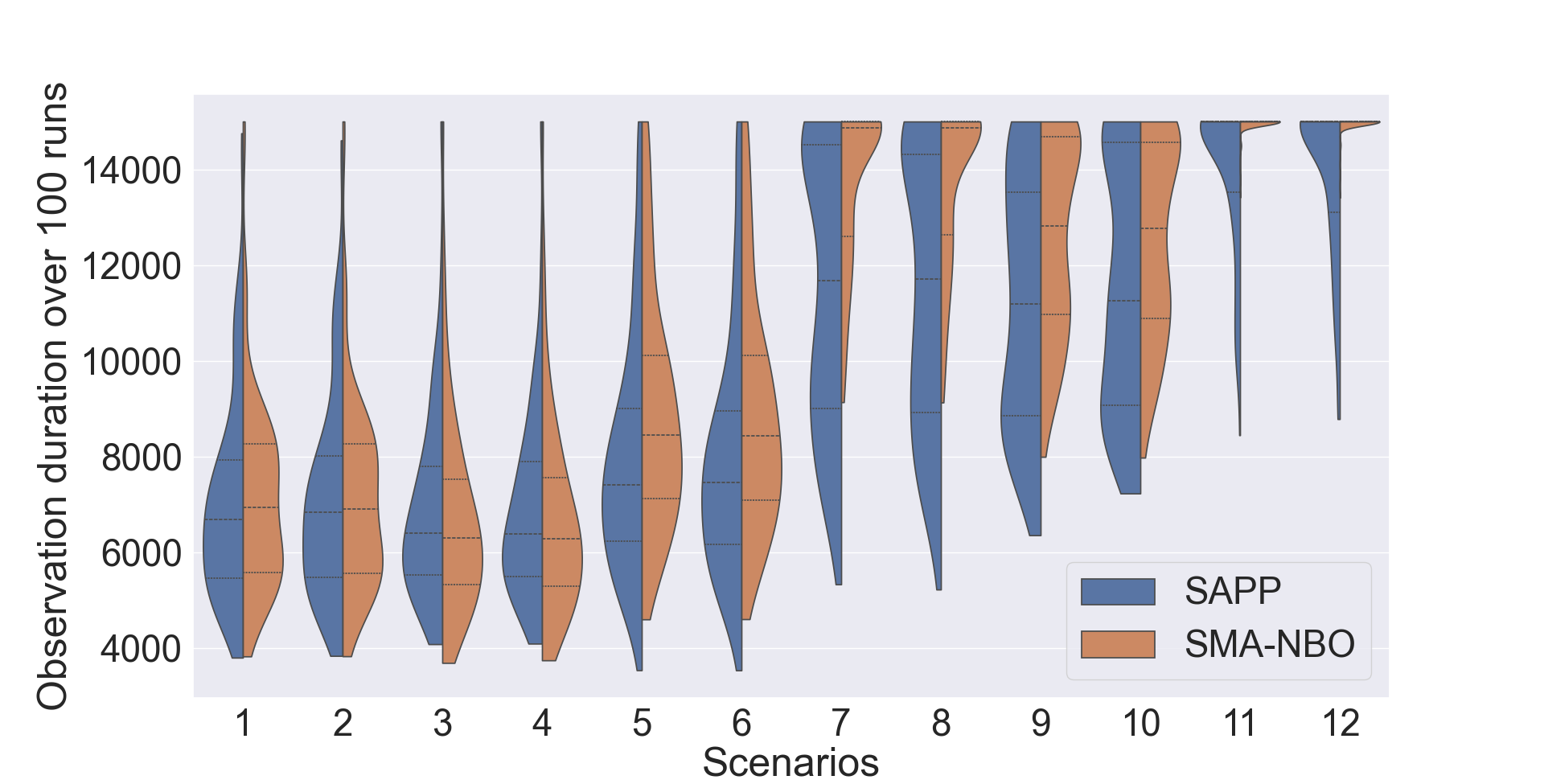
Figure 10: Violin plots for the comparison between SAPP and SMA-NBO in terms of observation duration. The violins indicate the actual distribution of the results over $100$ instances per scenario.

Table II and Figure 10 present how SAPP and SMA-NBO perform in different scenarios where we vary the camera number $|\mathcal{C}|$, the target number $|\mathcal{V}|$ and the time horizon length $H$. Shown are (per row) the results for $100$ instances; each instance's budget is $15,000$ time steps. The ``average observation duration'' refers to our objective: the average number of time steps needed (across all $100$ instances) to observe all targets once; lowest averages are highlighted in bold. The ``average execution time (s)'' refers to the computational cost in seconds per time step.

In almost all scenarios, SAPP observes all targets more quickly than SMA-NBO. In SAPP, the trajectories for all cameras are generated as soon as the proposed RML-based distributed path planning algorithm converges at an equilibrium solution, resulting in a per-step execution time that is longer than that of SMA-NBO. It is noteworthy that the execution time increases when we plan trajectories over a longer time horizon, i.e., $5$ time steps. Nevertheless the running time of SAPP is not too long, e.g., $1.170$ s when we plan paths for $30$ cameras over a $1$-time-step horizon to observe $50$ targets. It demonstrates that SAPP is not computationally expensive, and it can be deployed in real scenarios.

Table III: Results of Wilcoxon rank-sum test (p-value) and Cohen's d effect size for all scenarios. The former compares two groups of data without assuming any specific pattern in the data; a p-value of $0.01$ or less is considered as strong evidence for a difference. The latter characterises the practical benefits of SAPP over SMA-NBO: an absolute value $d=0.2$ is considered a ``small'' benefit, $0.5$ represents a ``medium'' benefit, and $0.8$ a large benefit.

Scenarios	p-value	Cohen's d effect size
$1$	$0.455$	$-0.03$
$2$	$0.636$	$-0.01$
$3$	$0.308$	$-0.13$
$4$	$0.296$	$-0.13$
$5$	$0.003$	$0.38$
$6$	$0.005$	$0.34$
$7$	$<0.001$	$0.93$
$8$	$<0.001$	$0.93$
$9$	$<0.001$	$0.57$
$10$	$0.008$	$0.43$
$11$	$<0.001$	$0.86$
$12$	$<0.001$	$0.91$

To further characterise the performance differences, we provide in Table III the outcomes of two statistical tests. As we can see, both approaches perform comparably on the smallest four scenarios. From Scenario $5$ on forward (i.e. from just 5 targets on), SAPP outperforms SMA-NBO with medium to large benefits in our favour.

VI Conclusion

In this paper, we have shown a sensor allocation and path planning approach to enhance the awareness of multiple targets in maritime situations. Here, the number of available sensors is lower than the number of targets while their FOV and detection range are limited. An optimization problem is formulated to distribute multiple sensors and plan paths for these sensors over a time horizon. Due to the complexity and large search space of this problem, we cope with it by developing two separate algorithms: a sensor allocation algorithm and a distributed path planning algorithm. The former relies on the sensor-target distance and the duration that targets have not been observed to allocate the sensors. The latter allows each camera to individually plan its trajectory to observe the targets.

Our experimental results show that compared to the existing solution, SAPP is efficient to minimize the duration to achieve situational awareness improvement under several different scenarios.

References

- [1] Australian Government: Departure of Home Affairs. (2023) Future Maritime Surveillance Capability. Accessed: 2023-05-18. [Online]. Available: https://www.homeaffairs.gov.au/how-to-engage-us-subsite/Pages/maritime-surveillance-capability-project.aspx
- [2] Australian Border Force. (2021) Maritime Border Command: Civil Maritime Security Threats. Accessed: 2023-05-18. [Online]. Available: https://www.abf.gov.au/about-us/what-we-do/border-protection/maritime/civil-maritime-security-threats
- [3] P. Zhou, W. Zhao, J. Li, A. Li, W. Du, and S. Wen, ``Massive Maritime Path Planning: A Contextual Online Learning Approach,'' IEEE Transactions on Cybernetics, vol. 51, no. 12, pp. 6262–6273, 2021.
- [4] J. Lin, P. Diekmann, C.-E. Framing, R. Zweigel, and D. Abel, ``Maritime Environment Perception Based on Deep Learning,'' IEEE Transactions on Intelligent Transportation Systems, vol. 23, no. 9, pp. 15 487–15 497, 2022.
- [5] A. Guerra, D. Dardari, and P. M. Djurić, ``Dynamic Radar Network of UAVs: A Joint Navigation and Tracking Approach,'' IEEE Access, vol. 8, pp. 116 454–116 469, 2020.
- [6] X. Lu, W. Yi, and L. Kong, ``Joint Online Route Planning and Resource Optimization for Multitarget Tracking in Airborne Radar Systems,'' IEEE Systems Journal, vol. 16, no. 3, pp. 4198–4209, 2022.
- [7] Ülkü Öztürk, M. Akdağ, and T. Ayabakan, ``A review of path planning algorithms in maritime autonomous surface ships: Navigation safety perspective,'' Ocean Engineering, vol. 251, p. 111010, 2022.
- [8] D. D. Bloisi, F. Previtali, A. Pennisi, D. Nardi, and M. Fiorini, ``Enhancing Automatic Maritime Surveillance Systems With Visual Information,'' IEEE Transactions on Intelligent Transportation Systems, vol. 18, no. 4, pp. 824–833, 2017.
- [9] D. Cormack, I. Schlangen, J. R. Hopgood, and D. E. Clark, ``Joint Registration and Fusion of an Infrared Camera and Scanning Radar in a Maritime Context,'' IEEE Transactions on Aerospace and Electronic Systems, vol. 56, no. 2, pp. 1357–1369, 2020.
- [10] Google Maps. (2023) Sydney Harbor. Accessed: 2023-02-08. [Online]. Available: https://www.google.com/maps/@-33.8503401,151.2364376,14.25z
- [11] International Maritime Organization. (2023) Accessed: 2023-02-08. [Online]. Available: https://www.imo.org
- [12] N. Takemura and J. Miura, ``View Planning of Multiple Active Cameras for Wide Area Surveillance,'' in Proceedings 2007 IEEE International Conference on Robotics and Automation, 2007, pp. 3173–3179.
- [13] S. Ragi and E. K. P. Chong, ``UAV Path Planning in a Dynamic Environment via Partially Observable Markov Decision Process,'' IEEE Transactions on Aerospace and Electronic Systems, vol. 49, no. 4, pp. 2397–2412, 2013.
- [14] Y. Bar-Shalom, F. Daum, and J. Huang, ``The probabilistic data association filter,'' IEEE Control Systems Magazine, vol. 29, no. 6, pp. 82–100, 2009.
- [15] Y. Kisialiou, I. Gribkovskaia, and G. Laporte, ``Supply Vessel Routing and Scheduling under Uncertain Demand,'' Transportation Research Part C: Emerging Technologies, vol. 104, pp. 305–316, 2019.
- [16] S. Capobianco, N. Forti, L. M. Millefiori, P. Braca, and P. Willett, ``Uncertainty-Aware Recurrent Encoder-Decoder Networks for Vessel Trajectory Prediction,'' in Proceedings of IEEE 24th International Conference on Information Fusion (FUSION), 2021, pp. 1–5.
- [17] S. Thombre, Z. Zhao, H. Ramm-Schmidt, J. M. Vallet García, T. Malkamäki, S. Nikolskiy, T. Hammarberg, H. Nuortie, M. Z. H. Bhuiyan, S. Särkkä, and V. V. Lehtola, ``Sensors and AI Techniques for Situational Awareness in Autonomous Ships: A Review,'' IEEE Transactions on Intelligent Transportation Systems, vol. 23, no. 1, pp. 64–83, 2022.
- [18] E. Chondrodima, P. Mandalis, N. Pelekis, and Y. Theodoridis, ``Machine learning models for vessel route forecasting: An experimental comparison,'' in 2022 23rd IEEE International Conference on Mobile Data Management (MDM), 2022, pp. 262–269.
- [19] Y. Yoon and Y.-H. Kim, ``Maximizing the Coverage of Sensor Deployments Using a Memetic Algorithm and Fast Coverage Estimation,'' IEEE Transactions on Cybernetics, pp. 1–12, 2021.
- [20] O. M. Alia and A. Al-Ajouri, ``Maximizing Wireless Sensor Network Coverage With Minimum Cost Using Harmony Search Algorithm,'' IEEE Sensors Journal, vol. 17, no. 3, pp. 882–896, 2017.
- [21] B. Zhang, J. Peng, and S. Li, ``Covering Location Problem of Emergency Service Facilities in an Uncertain Environment,'' Applied Mathematical Modelling, vol. 51, pp. 429–447, 2017.
- [22] N. Wang, Y. Gao, C. Yang, and X. Zhang, ``Reinforcement learning-based finite-time tracking control of an unknown unmanned surface vehicle with input constraints,'' Neurocomputing, vol. 484, pp. 26–37, 2022.
- [23] N. Wang, Y. Gao, Y. Liu, and K. Li, ``Self-learning-based optimal tracking control of an unmanned surface vehicle with pose and velocity constraints,'' International Journal of Robust and Nonlinear Control, vol. 32, no. 5, pp. 2950–2968, 2022.
- [24] N. Wang, Y. Gao, H. Zhao, and C. K. Ahn, ``Reinforcement Learning-Based Optimal Tracking Control of an Unknown Unmanned Surface Vehicle,'' IEEE Transactions on Neural Networks and Learning Systems, vol. 32, no. 7, pp. 3034–3045, 2021.
- [25] R. Praveen Jain, A. Pedro Aguiar, and J. B. d. Sousa, ``Target Tracking using an Autonomous Underwater Vehicle: A Moving Path Following Approach,'' in 2018 IEEE/OES Autonomous Underwater Vehicle Workshop (AUV), 2018, pp. 1–6.
- [26] C. Shi, L. Ding, F. Wang, S. Salous, and J. Zhou, ``Joint Target Assignment and Resource Optimization Framework for Multitarget Tracking in Phased Array Radar Network,'' IEEE Systems Journal, vol. 15, no. 3, pp. 4379–4390, 2021.
- [27] B. Cooper and R. V. Cowlagi, ``Interactive Planning and Sensing in Uncertain Environments with Task-Driven Sensor Placement,'' in 2018 Annual American Control Conference (ACC), 2018, pp. 1003–1008.
- [28] X. Lu, W. Yi, and L. Kong, ``Joint Online Route Planning and Resource Optimization for Multitarget Tracking in Airborne Radar Systems,'' IEEE Systems Journal, pp. 1–12, 2021.
- [29] C. Shi, X. Dai, Y. Wang, J. Zhou, and S. Salous, ``Joint Route Optimization and Multidimensional Resource Management Scheme for Airborne Radar Network in Target Tracking Application,'' IEEE Systems Journal, pp. 1–12, 2021.
- [30] K. Dogancay, ``UAV Path Planning for Passive Emitter Localization,'' IEEE Transactions on Aerospace and Electronic Systems, vol. 48, no. 2, pp. 1150–1166, 2012.
- [31] Z. Li, J. Xie, W. Liu, H. Zhang, and H. Xiang, ``Joint Strategy of Power and Bandwidth Allocation for Multiple Maneuvering Target Tracking in Cognitive MIMO Radar With Collocated Antennas,'' IEEE Transactions on Vehicular Technology, vol. 72, no. 1, pp. 190–204, 2023.
- [32] B. Floriano, G. A. Borges, and H. Ferreira, ``Planning for Decentralized Formation Flight of UAV fleets in Uncertain Environments with Dec-POMDP,'' in Proceedings of International Conference on Unmanned Aircraft Systems (ICUAS), 2019, pp. 563–568.
- [33] Y. Rizk, M. Awad, and E. W. Tunstel, ``Decision Making in Multiagent Systems: A Survey,'' IEEE Transactions on Cognitive and Developmental Systems, vol. 10, no. 3, pp. 514–529, 2018.
- [34] H. V. Nguyen, H. Rezatofighi, B. Vo, and D. C. Ranasinghe, ``Multi-Objective Multi-Agent Planning for Jointly Discovering and Tracking Mobile Objects,'' in The Thirty-Fourth AAAI Conference on Artificial Intelligence, AAAI 2020, New York, NY, USA, February 7-12, 2020. AAAI Press, 2020, pp. 7227–7235.
- [35] I. Chadès, L. V. Pascal, S. Nicol, C. S. Fletcher, and J. Ferrer-Mestres, ``A primer on partially observable Markov decision processes (POMDPs),'' Methods in Ecology and Evolution, vol. 12, no. 11, pp. 2058–2072, 2021.
- [36] T. Li, L. W. Krakow, and S. Gopalswamy, ``SMA-NBO: A Sequential Multi-Agent Planning with Nominal Belief-State Optimization in Target Tracking,'' in 2022 IEEE/RSJ International Conference on Intelligent Robots and Systems (IROS), 2022, pp. 5861–5868.
- [37] D. D. Nguyen, H. X. Nguyen, and L. B. White, ``Reinforcement Learning With Network-Assisted Feedback for Heterogeneous RAT Selection,'' IEEE Transactions on Wireless Communications, vol. 16, no. 9, pp. 6062–6076, 2017.
- [38] C. Fan, B. Li, C. Zhao, and Y. Liang, ``Regret Matching Learning Based Spectrum Reuse in Small Cell Networks,'' IEEE Transactions on Vehicular Technology, vol. 69, no. 1, pp. 1060–1064, 2020.
- [39] S. Hart and A. Mas-Colell, ``A simple adaptive procedure leading to correlated equilibrium,'' Econometrica, vol. 68, no. 5, pp. 1127–1150, 2000. [Online]. Available: https://onlinelibrary.wiley.com/doi/abs/10.1111/1468-0262.00153
- [40] X. Xu and Q. Zhao, ``Distributed No-Regret Learning in Multiagent Systems: Challenges and Recent Developments,'' IEEE Signal Processing Magazine, vol. 37, no. 3, pp. 84–91, 2020.
- [41] F. Sentenac, E. Boursier, and V. Perchet, ``Decentralized Learning in Online Queuing Systems,'' in Advances in Neural Information Processing Systems, vol. 34. Curran Associates, Inc., 2021.
- [42] G. E. Flaspohler, F. Orabona, J. Cohen, S. Mouatadid, M. Oprescu, P. Orenstein, and L. Mackey, ``Online Learning with Optimism and Delay,'' in 38th International Conference on Machine Learning, ser. Proceedings of Machine Learning Research, vol. 139, 18–24 Jul 2021, pp. 3363–3373.
- [43] I. Bistritz and N. Bambos, ``Cooperative Multi-player Bandit Optimization,'' in Advances in Neural Information Processing Systems, H. Larochelle, M. Ranzato, R. Hadsell, M. Balcan, and H. Lin, Eds., vol. 33. Curran Associates, Inc., 2020, pp. 2016–2027.
- [44] C. Daskalakis and N. Golowich, ``Fast Rates for Nonparametric Online Learning: From Realizability to Learning in Games,'' ser. STOC 2022. Association for Computing Machinery, 2022, p. 846–859.
- [45] I. Anagnostides, C. Daskalakis, G. Farina, M. Fishelson, N. Golowich, and T. Sandholm, ``Near-Optimal No-Regret Learning for Correlated Equilibria in Multi-Player General-Sum Games,'' in 54th Annual ACM SIGACT Symposium on Theory of Computing, 2022, p. 736–749.
- [46] B. L. Nguyen, D. D. Nguyen, H. X. Nguyen, D. T. Ngo, and M. Wagner, ``Multi-Agent Task Assignment in Vehicular Edge Computing: A Regret-Matching Learning-Based Approach,'' IEEE Transactions on Emerging Topics in Computational Intelligence, 2023, In press.
- [47] H. V. Nguyen, H. Rezatofighi, B.-N. Vo, and D. C. Ranasinghe, ``Online UAV Path Planning for Joint Detection and Tracking of Multiple Radio-Tagged Objects,'' IEEE Transactions on Signal Processing, vol. 67, no. 20, pp. 5365–5379, 2019.
- [48] J. Han, Y. Cho, J. Kim, J. Kim, N.-s. Son, and S. Y. Kim, ``Autonomous collision detection and avoidance for ARAGON USV: Development and field tests,'' Journal of Field Robotics, vol. 37, no. 6, pp. 987–1002, 2020.
- [49] Z. Tang and U. Ozguner, ``Motion planning for multitarget surveillance with mobile sensor agents,'' IEEE Transactions on Robotics, vol. 21, no. 5, pp. 898–908, 2005.
- [50] H. Huang, A. V. Savkin, and X. Li, ``Reactive Autonomous Navigation of UAVs for Dynamic Sensing Coverage of Mobile Ground Targets,'' Sensors, vol. 20, no. 13, 2020.
- [51] R. J. Aumann, ``Correlated equilibrium as an expression of bayesian rationality,'' Econometrica, vol. 55, no. 1, pp. 1–18, 1987. [Online]. Available: http://www.jstor.org/stable/1911154
- [52] SAFRAN. (2023) Vigy Observer/Engage HD. Accessed: 2023-02-18. [Online]. Available: https://www.safran-group.com/products-services/vigy-observerengage-hd-lightweight-and-stabilized-naval-daynight-observation-system