Strahler Number of Natural Language Sentences in Comparison with Random Trees

Abstract

The Strahler number was originally proposed to characterize the complexity of river bifurcation and has found various applications. This article proposes computation of the Strahler number’s upper and lower limits for natural language sentence tree structures. Through empirical measurements across grammatically annotated data, the Strahler number of natural language sentences is shown to be almost 3 or 4, similarly to the case of river bifurcation as reported by Strahler (1957). From the theory behind the number, we show that it is one kind of lower limit on the amount of memory required to process sentences. We consider the Strahler number to provide reasoning that explains reports showing that the number of required memory areas to process sentences is 3 to 4 for parsing (Schuler et al., 2010), and reports indicating a psychological “magical number” of 3 to 5 (Cowan, 2001). An analytical and empirical analysis shows that the Strahler number is not constant but grows logarithmically; therefore, the Strahler number of sentences derives from the range of sentence lengths. Furthermore, the Strahler number is not different for random trees, which could suggest that its origin is not specific to natural language.

Keywords— Strahler number; Tree structure; Memory

1 Introduction

The Strahler number (Strahler, 1957) was originally introduced in the field of geography, as a measure of the complexity of river bifurcation. Curiously, Strahler found that almost any river in England has a constant value of 4 for this number. Apart from geography, the Strahler number has been applied to analyze the complexity of computation trees in computer program source code (Ershov, 1958). In particular, it was theorized to equal the minimum number of memory areas that are necessary for evaluation of a computation tree (Ershov, 1958).

We believe that application of the Strahler number to natural language sentences can contribute, first of all, to understanding the Strahler number itself. Although the Strahler number has been reported to yield a value of four, various questions about it have not been fully answered: for example, what does this constant value signify apart from its definition, how does it grow with respect to the tree size, and what is the relation between random and real trees? In this work, we show that this number grows logarithmically with respect to the tree size. Furthermore, we empirically demonstrate that the Strahler number for natural, real trees is not different from that for random trees. In other words, the trees’ size range decides the Strahler number, which does not differ for random trees of the same size.

We believe that this understanding is important to natural language sentence structure, because multiple studies in psychology and natural language processing have empirically reported almost the same number, but without any theoretical grounding. Previous works on the structural characteristics of natural language sentences have focused on the cognitive load (Yngve, 1960; Kimball, 1975; Gibson, 2000; Liu et al., 2017). Cowan (2001) suggested a value of 3 to 5 for a “magical number” involved in cognitive short-term memory. Furthermore, in natural language processing of parsing methods, Schuler et al. (2010) indicated that human sentences require a maximum of four memory areas for a particular sentence. However, these previous works did not state why the number is four.

As will be shown here theoretically, the Strahler number of human sentences shows a kind of lower limit on the amount of memory necessary to understand sentence structure under a certain setting. We provide a mathematical definition of this lower limit and show that it is not actually a constant, but rather, it increases logarithmically with the sentence size. It is a fact, however, that sentence lengths can only take a certain range (Sichel, 1974; Yule, 1968), and this range is one factor in why the Strahler number is seemingly a constant. Furthermore, our work shows that this number is almost the same for random trees, thus providing a signification that the potential “magical number” might not be so “magical,” by explaining its origin via random trees.

2 Related Work

This work is related to four fields as follows. The first involves the general history of the Strahler number (Strahler, 1957). It was known in the literature before Strahler (Horton, 1945); however, we call it the “Strahler number” following convention. The Strahler number was analyzed from a statistical viewpoint in relation to the bifurcation ratio and area of a water field (Beer and Borgas, 1993). Meanwhile, it has found various applications besides river morphology, of which the most important is computer trees (Ershov, 1958), as mentioned above. That theory is the basis of this article, as explained in the following section.

The second genre of related work is measurement to characterize the complexity of natural language. Previously, there have been diverse approaches to consider this complexity. The primary approach is the Shannon entropy, which has seen numerous applications. Takahira et al. (2016) provided a summary, and the Shannon entropy was recently applied to characterize the specific field of legal texts (Friedrich, 2021). Apart from the Shannon entropy, various methods from statistical physics have also been applied to texts, including Zipf’s law (Zipf, 1949), long memory via methods such as long-range correlation (Altmann et al., 2009, 2012; Tanaka-Ishii and Bunde, 2016), and fluctuation analysis (Ebeling and Pöschel, 1993; Ebeling and Neiman, 1995; Kobayashi and Tanaka-Ishii, 2018; Tanaka-Ishii and Kobayashi, 2018). All of those works examined sequences, however, rather than sentence structure.

The study of sentence structure relates to the long memory phenomena of natural language. This is because one factor in long memory is the tree structure underlying a sequence: Lin and Tegmark (2017) analytically showed how a context-free grammar would produce long memory. More recent works have conjectured the nature of a formal grammar (Degiuli, 2019b, a), including whether it has phase changes. However, understanding of what kind of actual tree structure is the underlying cause of what kind of long memory will require more direct study of trees derived from real data. We believe that datasets of grammatically annotated sentence structures provide a good starting point.

For natural language sentence structure, there is a known bias in the branching direction in sentences, such as a right-branching preference in Indo-European (IE) languages (Forster, 1968). Such bias has been quantified in various ways, as excellently summarized in Fischer et al. (2021). One way to consider the complexity of this phenomenon is via the modifier-modified distances within a sentence (Gibson, 2000). Through an analysis of 20 languages, Liu (2008) reported that the dependency distance remains short but never reaches its theoretical minimum. More recent works have shown syntactic complexity based on various statistics acquired from sentence structure (Xu and Reitter, 2016; Yadav et al., 2020). The Menzerath law provides another quantitative approach to analyze the complexity of sentence structure. Specifically, the Menzerath conjecture of “the greater the whole, the smaller its parts” has been considered as a relation between the number and size of sentences’ main constituents in various languages (Tanaka-Ishii, 2021; Hou et al., 2017; Mačutek et al., 2017; Sanada, 2016; Buk and Rovenchak, 2007). In contrast, our work on the Strahler number takes a different approach from both of those quantitative methods applied to sentence structure.

The third genre of related work involves the amount of short-term memory as studied in the field of cognitive science. Among early works, Miller (1956) showed that the number of chunks in short-term memory is 7 $\pm$ 2. Yngve (1960) defined the complexity of dependency trees by their depth and argued that this depth is related to Miller’s number. Beyond language, Cowan (2001) argued that short-term memory is bounded by a “magical number” of 3 to 5. The exact nature of this short-term memory has been controversial. Our work provides a novel approach to explain this memory by using the Strahler number and its mathematical theory for random trees.

Lastly, this work relates to a genre of works in natural language processing on parsing. Every parsing study presents a method to reverse engineer a sentence structure. By applying such methods, some works showed the maximum amount of memory necessary for parsing. In particular, Schuler et al. (2010), and more recently Noji and Miyao (2014) indicated that processing human sentences require almost a maximum of three to four memory areas. This number has only been an empirical result, with no theoretical grounding. Hence, this work intends to explain this empirical result.

3 Strahler Number

3.1 Definition

Let $t=(V,E)$ denote a rooted directed tree, where $V$ is the set of nodes and $E\in V\times V$ is the set of edges. Each edge is directed from a parent to a child. Let $T$ denote the set of finite rooted directed trees, and let $n$ denote the number of nodes in a tree. Later, we will consider different sets as $T$: (1) dependency structures $U$ (Section 5), with $U(n)$ denoting the subset with $n$ nodes; (2) random binary structures $R_{2}(n)$ (Section 3.3); and (3) random $n$-node trees $R(n)$ (Section 4.2), as defined later.

Let a binary tree be one for which every inner node has two children. For a binary tree $t$, the Strahler number is defined in a bottom-up manner (Strahler, 1957; Horton, 1945). Every node $v$ acquires a Strahler number $S(v)$, and the Strahler number of the root is the Strahler number of the whole tree, $S(t)$. The definition is given as follows:

• For a leaf node $v$, $S(v)=1$.

• For an inner node $v$, let the two child nodes be $ch_{1}(v),ch_{2}(v)$.

  • If $S(ch_{1}(v))==S(ch_{2}(v))$, then $S(v)=S(ch_{1}(v))+1$.

  • Otherwise, $S(v)=\text{max}(ch_{1}(v),ch_{2}(v)).$

From this definition, the Strahler number is obviously unique for a given tree.

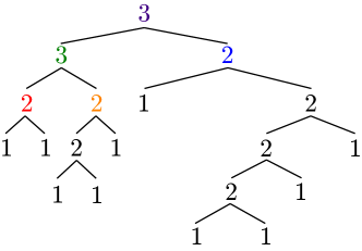
Figure 1: Strahler number of a tree.

Figure 1 shows an example tree with the values of $S(v)$ indicated for every node $v$. For instance, the node with the green “3” has two children. As the child nodes’ numbers are both 2, the parent node’s number is $2+1=3$. On the other hand, the root node with the purple number also has two children, one with a number of 3 (green) and the other with 2 (blue). Because the child nodes’ numbers are different, the Strahler number of the root is $\max(3,2)=3$. Through such bottom-up calculation, this tree’s Strahler number is calculated as 3.

3.2 Relation to Number of Memory Areas Required to Process Trees

After the Strahler number’s original definition to analyze river bifurcation in England, it was applied to analyze the complexity of computation trees (Ershov, 1958). A computation tree is produced from program code, which is parsed into a computation tree and then evaluated.

For example, Figure 4 shows a tree for a computation (i.e., program code) “$1+2*3^{4}$”. Parsing this program string generates the tree, which is then computed to yield 163. The question here is how much memory is necessary to get this result.

The Strahler number is known to give the minimum number of memory areas for tree evaluation by the use of shift-reduce operations (Sethi and Ullman, 1970), which constitute the simplest, most basic theory of computation tree evaluation. Here, we give a brief summary of these operations, with a more formal introduction given in Appendix C. A computation tree can be evaluated with the two operations of shift and reduce by using a memory system comprising a stack, which is a last-in, first-out (LIFO) data structure. A shift operation puts the data element of a tree leaf on the stack, and a reduce operation applies a functional operation (such as addition or multiplication) to the two elements at the top of the stack.

Figure 2: Computation tree for $1+2*3^{4}$.

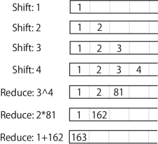
Figure 3: Transition of the stack during evaluation from the beginning of the tree.

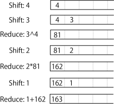
Figure 4: Transition of the stack during evaluation from the end.

For example, consider evaluation of the computation tree shown in Figure 4. For evaluation from the beginning of the tree, the required number of stack spaces is four, as shown in Figure 4. On the other hand, for evaluation from the end of the tree, the total number is reduced to two, as shown in Figure 4.

As seen here, which leaf of the tree is evaluated first determines the necessary depth of the stack. Every shift-reduce gives a way to traverse a given computation tree, and each way requires a particular number of stack space uses. Thus, there is a particular way to traverse a tree by the shift-reduce method that requires a minimum number of stack spaces.

This minimum number of stack spaces required to evaluate a computation tree equals the tree’s Strahler number (Ershov, 1958), which is obvious from the definition of the shift-reduce method as given in Appendix C. If no self-referential expression is involved, then this number is also the minimum number required for analyzing program code in a sequence represented as a computation tree. This is because analysis of a program as a computation tree is yet another way to traverse the tree.

To adapt this theory to natural language sentences, we can consider transformation of a sentence structure into a binary tree. The evaluation of this binary tree (to obtain some kind of meaningful representation) uses a certain memory amount. In describing this amount with use of the shift-reduce method, the necessary number of stack spaces for evaluation is bounded by the Strahler number. Because analyzing a sentence is equivalent to traversing a binary tree, the tree’s Strahler number gives the lower bound on the necessary number of stack spaces. This shift-reduce scheme is the simplest general method to deal with a sentence structure (Zhang, 2020). It has become a standard way to parse a sentence, and its use is an ongoing research topic (Fernández-González and Gómez-Rodríguez, 2019; Yang and Deng, 2020; Grenander et al., 2022; Fernández-González and Gómez-Rodríguez, 2023). Hence, knowledge of a sentence structure’s Strahler number can give a lower-limit criterion for the amount of memory required to process the sentence structure.

3.3 Strahler Number of Random Binary Trees with $n$ Leaves: $R_{2}(n)$

Before calculating the Strahler number of a sentence structure, we introduce the Strahler number of a random binary tree, which provides a good theoretical baseline.

Let $R_{2}(n)$ be the set of all binary trees with $n$ leaves. The set’s size $|R_{2}(n)|$ is known to be given by a Catalan number, i.e., $|R_{2}(n)|=\frac{1}{n}{}_{2n-2}C_{n-1}$ (Stanley, 2015).

Flajolet et al. (1979) analytically showed that the mean Strahler number can be deductively described via approximately logarithmic growth with a base of four, and the mean value obviously increases with the tree size $n$. Later, this theoretical fact will provide an important reference in understanding the complexity of natural language sentences.

In addition to the Strahler number’s mean behavior, its upper and lower limits can be considered. For a given set of trees, $T$, the upper/lower limits are respectively defined as the maximum/minimum Strahler numbers. Hence, we analytically consider the upper/lower limits for $R_{2}(n)$. By the definition of the Strahler number, the upper limit is obviously acquired from a tree that is closest to a complete tree (Ehrenfeucht et al., 1981), where the Strahler number equals the tree’s maximum depth. Therefore, the upper limit for $R_{2}(n)$ is $\lfloor\log_{2}{n}\rfloor+1$. On the other hand, the lower limit derives from the opposite case of a tree that is closest to a linear tree. Specifically, the lower limit is 1 for $n=1$, or 2 otherwise, because for $n>1$, there are two leaf nodes and all inner nodes thus have a Strahler number of 2.

4 Measurement of Strahler Number of Sentence Structure

There have been two main paradigms in representing tree structures: phrase structure (Chomsky, 1956) and dependency structure (Tesnière, 1959). Here, we use these terms under the most conventional definitions, but briefly, the former describes natural language sentences in a similar manner to a computation tree, as described above, where words are located at leaves and inner nodes describe the relations between words. On the other hand, the latter describes a tree structure as the modifier-modified relations among words. In other words, the inner nodes of the tree in the phrase structure paradigm are not words, whereas those in the dependency structure paradigm are words.

In this article, we calculate the Strahler number with a dependency structure rather than a phrase structure, because a large amount of annotated data is available in a large number of languages, as with the data that will be described in Section 5. Hence, the question here is how to calculate the Strahler number for every dependency tree.

In Section 3.1, the Strahler number was defined for a binary tree, whose inner nodes and leaf nodes are different, with only leaf nodes representing words. On the other hand, both the inner and leaf nodes of a dependency structure are words, with inner nodes having multiple child nodes for modifiers. Filling of the gap between the differences in these two settings would suggest only two directions: to transform dependency structures into binary phrase structure trees; or to extend the Strahler number by adapting it to the dependency structure.

Regarding the latter direction, there have been previous attempts to extend the Strahler number to general trees with nodes having more than two children (Auber et al., 2004). The method in that work extended the rule to count up the Strahler number at each bifurcation as described in Section 3.1. However, we do not adopt this generalization, mainly because the theory around it is not established. The theory on computation trees would not apply easily; in addition, the analytical theory for random binary trees would not be easy to extend to general trees.

Hence, in the following, we consider methods to transform dependency trees into binary trees to calculate the Strahler number. First, we explain two particular binarization methods. Later, in the experimental section (Section 6), we show that these two methods yield very similar results with respect to the Strahler number. Second, we provide a method to acquire the upper and lower limits across any binarization method. The results for any particular binarization method fall within the range between the upper and lower limits, and the limits can be compared with those of random trees.

4.1 Two Binarization Methods for Dependency Structure

The transformation of a dependency structure to a phrase structure is not easy (Kong et al., 2015; Fernández-González and Martins, 2015), partly because the grammatical attribute of every inner node must be estimated, whereas the reverse transformation is relatively feasible (Buchholz, 2002). Here, we want to effectuate this difficult transformation but without requiring any precise prediction of the attributes of inner nodes, as we want to calculate the Strahler number gregardless of its specific value.

We transform a given dependency structure via the following two methods:

• Transformation by use of a manually crafted grammar (Tran and Miyao, 2022).

• Transformation without a grammar, by use of heuristics.

Binary1 derives from a grammar proposed by Reddy et al. (2017). The grammar describes the degree of grammatical relation between the modifier and modified, and the dependency tree is binarized on the order of this degree. For an explanation of this grammar, see Reddy et al. (2017).

On the other hand, Binary2 binarizes a dependency structure via two simple heuristics based on a modifier’s distance from the head. The two heuristics are as follows: (1) the modifiers before the head are bifurcated then those after; (2) the farther modifiers from the head are bifurcated earlier than those closer. Although these are heuristics, this method has a relation to the linguistic theory of center embedding of sentences.

(a) Dependency structure example

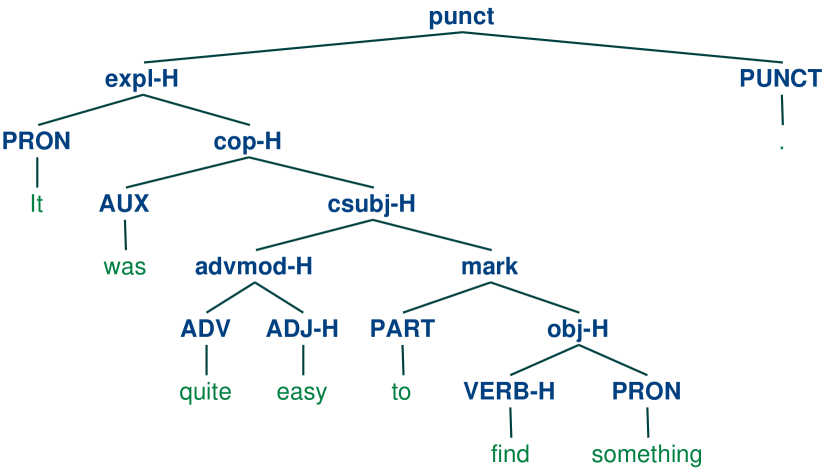
(b) Binary1 of (a), using grammar

(c) Binary2 of (a), using heuristics

Figure 5: Dependency structure (a) and binary phrase structures (b, c) of "It was quite easy to find something." (a) is an example from the Universal Dependency Dataset (Nivre et al., 2020c).

A binarization example is shown in Figure 5, in which (a) shows the tree of an original dependency structure, and (b) and (c) show its binary-transformed phrase structure trees obtained with Binary1 and 2, respectively.

As seen through these examples, the binarization methods each have pros and cons. Binary1 has an advantage in that the resulting tree structure reflects the correct sentence structure, but as mentioned above, its applicability is limited. On the other hand, Binary2 does not strictly reflect the sentence structure, but it is always applicable. After application of Binary1 and 2, each tree’s Strahler number can be obtained by following the definition.

4.2 Upper/Lower Limits of Strahler Number for Dependency Structures and Random Trees with $n$ Nodes: $R(n)$

Binary1 and 2 are examples of possible methods for transforming a dependency tree to a binary tree. Because the resulting Strahler number depends on the resulting set of trees acquired via the transformation method, we want to obtain the number’s upper and lower limits for all possible binary transformation methods.

In other words, a dependency tree $u_{x}$ can be transformed into various binary trees by using some method under conditions that reflect the original dependency structure. Let $U_{x}$ be the set of all binarized trees for a given $u_{x}$, where each element is a binary tree obtained with a particular binarization method. The upper and lower limits are the maximum and minimum of Strahler numbers, respectively, in $U_{x}$.

The details of obtaining the upper/lower limits are described in Appendix A, but we provide a summary here. A binarization method constitutes a method to binarize each inner node $v$ of a tree $t$. Binary1 and 2 are examples of different strategies, using a grammar or heuristics. At each inner node, there is a binarization method that maximizes or minimizes the Strahler number $S(v)$. The maximizing method binarizes the subtree under $v$ so that it becomes closer to a complete tree, whereas minimization makes the subtree closer to a linear tree. We showed a very similar argument in Section 3.3 for random trees. The maximum and minimum can be calculated inductively to acquire the Strahler number’s respective upper and lower limits. Note that these limits are obtained while ignoring the word order and the constraint of non-intersection, because the maximum and minimum at each node $v$ are difficult to compute under these constraints.

Thus far, we have explained how to acquire the upper/lower limits for a particular tree $u_{x}$. We can also get the upper/lower limits across the $u_{x}$ in a set of $U$. Specifically, for each subset $U(n)$ of trees with $n$ nodes, the mean upper/lower limits of $U(n)$ can be computed.

These upper and lower limits are comparable with those for the set of random binary trees, $R_{2}(n)$, as mentioned in Section 3.3. Furthermore, apart from $R_{2}(n)$, we can consider another set of random trees: all possible trees with $n$ nodes, denoted as $R(n)$. The mean upper/lower limits of $R(n)$ for each $n$ are also empirically computable by the same method described in this section. Because $|R(n)|$ is also a Catalan number (Stanley, 2015), computation of the upper/lower limits of $R(n)$ requires dynamic programming to cover the entire set. We summarize that approach in Appendix B and give the details in Appendix D.

5 Data

For the set $U$, as mentioned above, we use Universal Dependencies (de Marneffe et al., 2021; Nivre et al., 2020c), version 2.8, to measure the Strahler number for natural language. Universal Dependencies is a well-known, large-scale project to construct large-scale annotated data for natural language sentences. The annotation is defined under the Universal Dependency scheme, which is a representation based on dependency structure. The version used in this article contains 202 corpora across 114 languages. The corpora are listed in table 2 of Appendix E.1. Binary1 and 2 can be applied and upper and lower limits can be calculated for all these data.

6 Results

To summarize the approach thus far, we have a dependency dataset $U$, in which the subset of trees of size $n$ is denoted as $U(n)$. For random trees, we have a set of binary random trees with $n$ leaf nodes, denoted as $R_{2}(n)$, and a set of random trees with $n$ nodes, $R(n)$.

As described above, for $R_{2}(n)$, the theoretical mean and upper and lower bounds of the Strahler number are analytically known. For the other sets, these values must be acquired empirically. For a tree $t$ belonging to one of those sets, we calculate the upper/lower limits of Strahler numbers. In terms of $n$, the averages of each of these four values can be acquired for $U(n)$ and $R(n)$. Binary1, 2 can also be calculated for $U(n)$.

In this section, we consistently use color as follows. For $R_{2}(n)$, we use black for the upper/lower limits and the mean, green for Binary1, and blue for Binary2. For $U(n)$, we use pink for the upper limit and red for the lower limit. For $R(n)$, we use purple for the upper limit and orange for the lower limit.

Table 1: Average $\pm$ standard deviation of the Strahler numbers for all dependency trees.

	All dependency trees
Upper limits	$3.56\pm 0.83$
Lower limits	$2.71\pm 0.60$
Binary1 (with Grammar)	$3.21\pm 0.74$
Binary2 (with heuristics)	$3.11\pm 0.70$

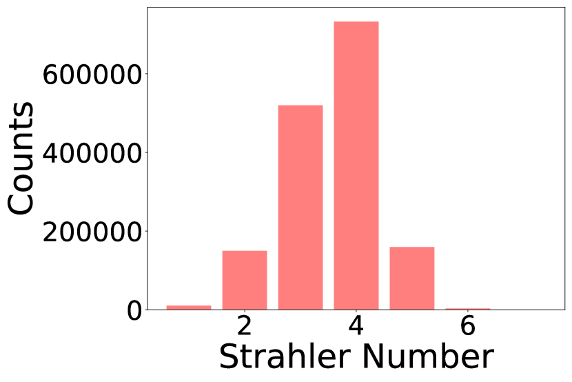
(a) Upper limits

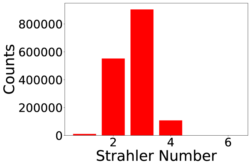
(b) Lower limits

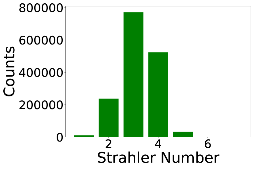
(c) Binary1

(d) Binary2

Figure 6: Histogram of the Strahler numbers of dependency trees.

6.1 Strahler Number of Sentence Structure

Table 1 lists the means and standard deviations for the entire dependency dataset. We see that the average Strahler number of a dependency structure is usually less than 4. The Binary1 and Binary2 values are between the upper and lower limits. For each corpus, the specific means and standard deviations for Binary1 and 2 and the upper/lower limits for $U(n)$ are listed in Appendices E.2-E.5, Tables 3-10.

Figure 6 shows a histogram of the Strahler numbers. It can be seen that the distribution shifts from large to small in the order of the upper limit, Binary1, Binary2, and the lower limit. Note that Binary1 and 2 show pretty similar results, regardless of the binarization method. The median Strahler number is 4 for the upper limit, and 3 for all other cases. Strahler numbers larger than 4 are clearly very scarce.

The dependency dataset includes data of various language groups, genres, and modes (speech/writing). According to our analysis, the differences with respect to Strahler number among datasets are not distinct across this variety of data. The largest Strahler number is 7, and the smallest is 1. Examples of both extremes are given in Appendix F. The examples with a number of 1 are mainly one-word salutations, interjections, and names (even without periods; Appendix F, Table 11). On the other hand, sentence examples with a Strahler number of 7 are very rare and contain a large number of words. As seen here, sentences with a larger Strahler number above 4 are atypical and include examples for which it might be questionable to call them sentences. The dependency dataset includes such questionable entries, and the Strahler number could provide evidence to quantify such irregularities in the corpora.

6.2 Growth of Strahler Number w.r.t. Sentence Length

Originally, when the Strahler number was used for analysis of rivers in England, it was found to be 4. We can also conclude from the previous section that the Strahler number for sentence structure is almost 4. This leads us to wonder how this number is significant. Thus far, we have discussed the Strahler number as a constant value with a given distribution. In the following, we show that it is not a constant but merely looks like a constant, because it grows slowly with respect to $n$, and the range of sentence lengths is limited. In fact, the number depends on the logarithm of the tree size $n$.

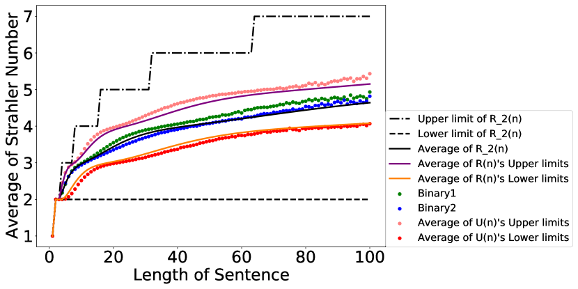
Figure 7: Average Strahler number with respect to the tree size $n$.

Figure 7 shows the mean results for the tree sets $U(n)$, $R_{2}(n)$, and $R(n)$, as summarized at the beginning of this section. The black analytical lines for $R_{2}(n)$ indicate the exact values following the theory explained in Section 3.3. For the other sets, the plots show empirical results measured across trees of size $n$. All plots approximately increase logarithmically, but none of them are smooth, as they have a step at $n=2$, and they globally fluctuate by changing their logarithmic base. Overall, the necessary number of stack spaces is bounded by the logarithm of the tree size.

For each $n$, the possible range of Strahler numbers for $R_{2}(n)$, which extends between the upper and lower black lines, is obviously far wider than the range for $U(n)$. On the other hand, the range for $U(n)$ is between the pink and red points. The range for $R(n)$ is between the purple and orange lines, which is slightly narrower than the range for $U(n)$, despite $R(n)$ being the average of all random trees with $n$ nodes.

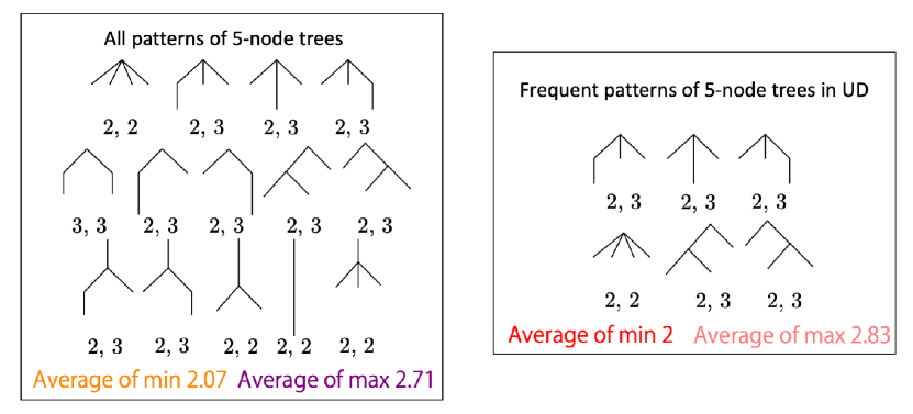
Figure 8: Sample trees for $n=5$: (left) all possible trees, and (right) tree structures appearing frequently among Universal Dependency (UD) trees. Two numbers beneath each tree indicate the mininum and maximum, respectively, of the Strahler number across all possible binarialization methods.

These results can be understood from a small example. Figure 8 shows a set of trees of size $n=5$, with all such possible trees on the left, and typical structures appearing frequently in the dependency dataset on the right. The distribution of tree shapes in the dataset varies, with the set of trees on the right accounting for 80% of the total. The upper and lower limits of the Strahler number are listed below each tree. The averages are listed at the bottom of each box in the corresponding colors from the scheme used throughout this section. For $R(n)$, the respective upper/lower limits are 2.71 and 2.07; in contrast, if the six trees on the right appeared equally, the upper/lower limits would be 2.83 and 2. Thus, the range of $R(n)$ is narrower than that of $U(n)$, even in this small sample with $n=5$.

The actual plots in Figure 7 were obtained by computing the average across the distribution of shapes, but the range of $R(n)$ is still contained within that of $U(n)$. This small example with $n=5$ explains why the range of $R(n)$ can be almost the same or even smaller than that of $U(n)$: the Strahler number is mostly the same for any kind of tree of the same size and does not especially characterize the tree shape.

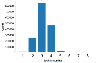
Figure 9: Histogram of the Strahler numbers of random trees from $R_{2}(n)$, when sampling $n$ from the distribution of Binary 1.

To show how the Strahler numbers of natural language trees are not much different from those of random trees, we can examine a histogram of the results for $R_{2}(n)$, the null model. Because any arbitrary large tree of size $n$ can be generated for $R_{2}(n)$ and the Strahler number grows with respect to $n$, trees lengths were sampled from Binary1, and for each $n$, a Strahler number was sampled from the population of $R_{2}(n)$. Figure 9 shows a histogram of $R_{2}(n)$ for the total number of sentences in UD. In comparison with Figure 6(c), there are more trees here with a Strahler number of 3. The Strahler number’s average and standard deviation were $3.15\pm 0.70$ here, a little smaller than for Binary1. Thus, the results do not show much difference between random trees and natural language trees.

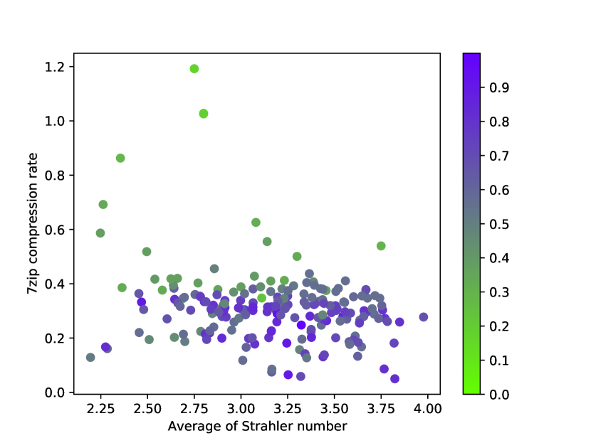
Figure 10: 7zip compression rate with respect to the average Strahler number per corpus for Binary1.

6.3 Difference of Strahler Number from Compression Factor

To investigate the Strahler number’s significance further, this section demonstrates its originality in terms of how it differs from other complexity measures.

First, although the Strahler number depends on the logarithm of the tree size $n$, the depth and Strahler number are different. Previously, a tree’s depth was considered as a kind of tree complexity, as in Yngve (1960), but a tree’s depth does not necessarily signify sentence complexity. For example, a linear tree of size $n$ has a deptch of $n$, yet its Strahler number is 2. The Strahler number is a much more sophisticated statistic related to the amount of necessary memory, as argued above in this article. Theoretically, the Strahler number’s dependence almost on the logarithm of the tree size is not trivial, as demonstrated in Flajolet et al. (1979)’s analytical work. Experimentally, the Strahler number requires actual, nontrivial calculation, which has been the main point of this work.

Another representative complexity measure that has frequently been applied to quantify natural language text is the Shannon entropy (Shannon, 1948). Other, entirely different characteristics could have some correlation with the Shannon entropy. For example, Takahashi and Tanaka-Ishii (2019) showed how Taylor’s exponent, which quantifies fluctuation, has an empirical relation with the perplexity, another form of the Shannon entropy. The remainder of this section shows that the Strahler number does not correlate with the Shannon entropy and thus captures a different aspect of natural language complexity.

Tanaka-Ishii and Aihara (2015) showed how direct calculation of the Shannon entropy depends on the corpus length if it is calculated via the plug-in entropy, $-\sum_{i}p(w_{i})\log(w_{i})$, with the $w_{i}$ being elements, i.e., either words or characters. This dependence on the corpus length is alleviated by using a good compression method $\gamma$ to calculate the compression rate $r=|D|/|\gamma(D)|$, where $D$ is the original corpus, $\gamma(D)$ is the compressed version, and $|\cdot|$ denotes a sequence’s length. The compression rate $r$ is theoretically proven to tend to the true Shannon entropy, provided that $\gamma$ is universal, and that $D$ is stationary and ergodic (Cover and Thomas, 1991). Friedrich (2021) applied the same strategy to compress texts and thus examine the complexity of domain-specific texts. Furthermore, Takahira et al. (2016) showed that, among different compression methods, the PPM (Prediction by Partial Match) method (Bell et al., 1990) behaves correctly following theory at least for some random data with a much faster compression speed relative to the text length than other popular methods such as Lempel-Ziv.

Given previous reports above, for every corpus in Binary1, we compared the average of the Strahler number and the PPM compression rate for text sequences taken only from grammatically annotated corpora.

Figure 10 shows the results. Every point corresponds to a UD corpus, with the horizontal axis indicating the average Strahler number, and the vertical axis indicating the compression rate. The values on the horizontal axis correspond to the values mentioned in Appendix E.2. To illustrate the influence of the corpus length on the compression rate, the points have colors ranging from blue (or purple) to green in terms of the ratio of the logarithm of each corpus’ number of sentences to the logarithm of the number of sentences in the largest corpus of UD. As seen in the figure, the green points (representing very small corpora) are located toward the top, whereas the majority of the blueish (purplish) points (larger corpora) are not necessarily correlated with their vertical locations. Thus, we believe that the text length’s influence on the compression rate is insignificant. Note that if we directly use the Shannon plug-in entropy, the length does influence the location, because the UD corpora are limited in size.

As seen in Figure 10, the compression rate is scattered almost the same for any Strahler number. This shows that the Strahler number is independent of the compression rate, and captures a different aspect of the complexity of language structure than the Shannon entropy. . Whereas the Shannon entropy highlights the complexity over a sequence, the Strahler number indicates the complexity of the memory required to process a tree structure, and this figure shows how these two measures are essentially different. We consider this article’s value to lie in investigating the Strahler number’s behavior as known in statistical physics while revealing another aspect of the complexity of natural language.

7 Discussion

Previous reports on the maximum number of short-term memory areas that can be cognitively used have consistently suggested a value of 3 to 5. In a survey of previous works, Cowan (2001) summarized cognitive works that tested the maximum number of events or instances that could be remembered through human psychological experiments, e.g., via instant memory (Sperling, 1960) or graphics (Luck and Vogel, 1997). Cowan stated that the number of such memory areas is 3 to 5 and referred to the value as a “magical number.”

The possible relation of such a maximum number of short-term or local memory areas to the number of memory areas required for sentence understanding is nontrivial. Memory is necessary to understand sentences, and one model for theorizing this could be based on the shift-reduce approach, as presented in this work. Under this setting, the experimental results in this article shows that this number is within the range of Cowan’s magical number.

In parallel to these findings in psychology, there have been works on parsing sentences, as mentioned in the Related Work section. Some works reported the maximum number of memory areas to process a sentence. Although the number depends on the parsing method, the works since Schuler et al. (2010) have reported the number to be three to four, as we have found here.

Hence, our work’s contribution is reasoning about this magical number in a rigorous setting via the lower limits of shift-reduce evaluation of a tree. Although our findings are limited to this setting, we have shown that the Strahler number grows with the logarithm of the sentence length. Conjecturing on the similarity and distinction of parsing techniques and our work, we predict that the lower limit of the memory amount necessary to process human sentences by parsing also grows logarithmically. Then, the reason why this number is three to four lies in the range of sentence lengths: because a logarithmic function grows slowly, a large range falls into a logarithmic value of three to four.

Furthermore, through a comparison with random trees from $R(n)$, we have shown that this result is not specific to human sentences but applies in general to a wider set of all possible random tree shapes. This understanding suggests the possibility that the magical number is not specific to human-generated trees but could derive from the behavior of trees in general.

8 Conclusion

In this article, we examined the use of the Strahler number to understand the nature of sentence structure. The Strahler number was originally defined to analyze the complexity of river bifurcation. Here, we applied it to sentences, which is the first such application to the best of our knowledge. Because the tree structure dataset used here is much larger than the datasets used in previous applications, it enabled a statistical study of the Strahler number in comparison with random trees.

The Strahler number entails the memory necessary to process a sentence structure via the basic shift-reduce method. We proposed ways to compute a sentence’s Strahler number, via two binarization methods and the upper and lower limits across all possible binarization methods. The experimental results showed that the Strahler number of a natural language sentence structure is almost 3 or 4. This number was found to grow with the sentence length, and the upper/lower limits were found to be close to those of random trees of the same length, which is the Strahler number’s key characteristic with respect to trees, including random trees. These findings provide evidence and understanding of the memory limit discussed to date in relation to the “magical number” in psychology and the upper limit on the memory necessary to parse texts.

Appendix A Upper/Lower Limits of $n$-Node Dependency Tree

Given a dependency tree $t$, for a word in node $v$, let $f_{\max}(v)$ and $f_{\min}(v)$ be functions that obtain the maximum and minimum Strahler numbers, respectively. These functions give the maximum and minimum across any binarization of $t$.

Both $f_{\max}(v)$ and $f_{\min}(v)$ are calculated using the following function $it(x,y)$:

$$it(x,y)=\left\{\begin{aligned} &x+1&&\textrm{if }x==y\\ &\max{(x,y)}&&\textrm{otherwise}\end{aligned}.\right.$$

Note that this function is almost the same as the definition of the Strahler number given in Section 3.1.

Using this function, the upper and lower limits are calculated in a bottom-up manner from the leaves to the root. Let $a\Leftarrow b$ denote a computational substitution. The calculations of the upper/lower limits, which proceed similarly, are defined below on the left/right, respectively:

Upper limit

$f_{\max}(v)$ is computed as follows.

• For a leaf node $v$, $f_{\max}(v)\Leftarrow 1$.

• For an inner node $v$, $f_{\max}(v)$ is calculated by the following four steps, where CH$(v)$ is the set of children of $v$ in the dependency tree.

  1. Sort CH$(v)$ in ascending order of $f_{\max}(v^{\prime})$, $v^{\prime}\in$CH$(v)$. Let $ch_{i}\in$CH$(v)$, $i=1,\ldots,|$CH$(v)|$, denote the $i$th child in this order.

  2. Set $f_{\max}(v)\Leftarrow 0$ (Initialization).

  3. $f_{\max}(v)\Leftarrow it(f_{\max}(v),1)$ (Upper limit should always count as 1).

  4. For $ch_{i}\in$ CH$(v)$, repeat in order of $i$, as follows:
        $f_{\max}(v)\Leftarrow it\left(f_{\max}(v),f_{\max}(ch_{i})\right)$.

Lower limit

$f_{\min}(v)$ is computed as follows.

• For a leaf node $v$, $f_{\min}(v)\Leftarrow 1$.

• For an inner node $v$, $f_{\min}(v)$ is calculated by the following four steps, where CH$(v)$ is the set of children of $v$ in the dependency tree.

  1. Sort CH$(v)$ in descending order of $f_{\min}(v^{\prime})$, $v^{\prime}\in$ CH$(v)$. Let $ch_{i}\in$CH$(v)$, $i=1,\ldots|$CH$(v)|$, denote the $i$th child in this order.

  2. Set $f_{\min}(v)\Leftarrow 0$ (Initialization).

  3. For $ch_{i}\in$ CH$(v)$, repeat in order of $i$, as follows:
         $f_{\min}(v)\Leftarrow it\left(f_{\min}(v),f_{\min}(ch_{i})\right)$.

  4. $f_{\min}(v)\Leftarrow it(f_{\min}(v),1)$ (Function $it$ should be considered for node $v$).

Appendix B Calculation of Average Upper/Lower Limits of $R(n)$

This section briefly describes how to compute the average upper or lower limit of $R(n)$. The method’s precise details are given in Appendix D. For a given set of trees, $R(n)$, let $R_{n,p_{\max}}$ be the total number of trees of size $n$ with an upper limit $p_{\max}$, and let $R_{n,p_{\min}}$ be the same with a lower limit $p_{\min}$.

The average upper and lower limits, respectively denoted as $R_{\max}(n)$ and $R_{\min}(n)$, are calculated as follows:

• Upper limit:

  $$R_{\max}(n)=\frac{\sum_{p_{\max}}p_{\max}R_{n,p_{\max}}}{\sum_{p_{\max}}R_{n,p_{\max}}}.$$

• Lower limit:

  $$R_{\min}(n)=\frac{\sum_{p_{\min}}p_{\min}R_{n,p_{\min}}}{\sum_{p_{\min}}R_{n,p_{\min}}}.$$

Hence, it becomes necessary to enumerate $R_{n,p_{\max}}$ and $R_{n,p_{\min}}$ through dynamic programming. The details are explained in Appendix D.

Appendix C Relations Among Shift-Reduce Method, Sethi-Ullman Algorithm (Sethi and Ullman, 1970), and Strahler Number

A computation tree is evaluated by use of the two operations of shift and reduce. The optimal sequence of operations to minimize the number of stack space uses is given by the Sethi-Ullman Algorithm (Sethi and Ullman, 1970). As mentioned in the main text, Ershov (1958) showed that the minimum number of stack space uses equals the Strahler number. This section clarifies the relations among the shift-reduce method, the Sethi-Ullman algorithm (Sethi and Ullman, 1970), and the Strahler number.

Shift-reduce method

The shift-reduce algorithm is an algorithm for using a stack (a LIFO structure) to evaluate a computation tree. The tree is a binary tree in which each leaf node stores data and each inner node is a function that combines the values of its two children.

The shift and reduce operations are defined as follows:

• Shift Put a leaf from the unanalyzed part of the tree on the top of the stack.

• Reduce Remove the top two elements from the stack and combine them into a single component according to the function in the corresponding inner node; then, put the result on the top of the stack.

Sethi-Ullman algorithm

The Sethi-Ullman algorithm is a depth-first evaluation method using registers for memory. The use of registers when applying a depth-first strategy to an evaluation tree is a LIFO process. The Sethi-Ullman algorithm preprocesses a given evaluation tree by annotating each node with a value, in an equivalent manner to the Strahler number, as follows:

1. Assign a value $x(v)$ for each node $v$.

   • If node $v$ is a leaf, $x(v)\Leftarrow 1$.

   • If node $v$ is an inner node, let its two children be $v1,v2$.

     • If $x(v1)=x(v2)$, then $x(v)\Leftarrow x(v1)$.

     • Otherwise, $x(v)\Leftarrow$ max$(x(v1),x(v2))$.

2. The tree evaluation is conducted depth-first, by always first evaluating the child $v$ with the larger $x(v)$.

Sethi and Ullman (1970) proved that this algorithm minimizes the number of registers used for evaluation.

Appendix D Calculation of Average Upper/Lower Limits of $R(n)$

Here, we explain the details of the method given in Appendix B to calculate the averages of the respective upper and lower limits, $R_{\max}(n)$ and $R_{\min}(n)$, of $R(n)$. The calculation uses dynamic programming for the upper/lower limits by enumerating $R_{n,p_{\max}}$ and $R_{n,p_{\min}}$, respectively. Because the dynamic programming proceeds in the same manner for both cases, the method is explained here for $R_{n,p}$, where $p$ indicates either $p_{\max}$ or $p_{\min}$. Furthermore, for a node $v$, we use the function $f(v)$ as defined in Appendix A to denote the corresponding $f_{\max}(v)$ or $f_{\min}(v)$.

For a given tree $t$, let $\#t$ denote its size and $r(t)$ denote its root node. For node $v$ in tree $t$, let CH$(v)$ denote the set of children of $v$. Let $Q(t)$ be

$$Q(t)=\{f(ch)|ch\in\mathrm{CH}(r(t))\}.$$

Here, $Q(t)$ is a set of integers acquired as limits on the children of $r(t)$. For each $Q(t)$, a Strahler number can be computed. Calculation of the limits requires consideration for $\forall t\in R(n)$, but $|R(n)|$ is a Catalan number, and the enumeration is thus difficult. One strategy is to consider trees with the same Strahler number as a certain type, which can be obtained from $Q(t)$ as follows.

Figure 11: Illustration of the equality of Strahler numbers for states having the same integer more than twice. The left side shows a dependency tree $t$ with 4 children whose Strahler number are same. For this tree $t$, $Q(t)=\{\cdots a,a,a,a,b\cdots\}$, and $Q^{\prime}(t)=\{\cdots a,a,b\cdots\}$. Note that the elements of $Q(t)$ are sorted in either ascending or descending order as described in Appendix A; therefore, instances of the same number will always appear together in the set. Instances of an integer appearing more than twice in $Q(t)$ can be removed, enabling reduction to $Q^{\prime}(t)$, as follows. The right side of the figure shows the binary tree of $t$. The Strahler numbers of the first two nodes are $a$ and $a+1$, but after the second node from the left, the Strahler numbers are all $a+1$. This example shows how integer instances appearing more than twice can be eliminated. This reduction is essential to deal with the Catalan number size of $R(n)$.

As explained in Appendix A for the procedures to calculate the upper/lower limits, the elements of $Q(t)$ are sorted in ascending/descending order, and instances of the same integer element will thus appear together. If the sorted $Q(t)$ has more than two instances of the same integer, such as 1 in $Q(t)=\{1,1,1,1,2,3\}$, then half those instances can be removed, yielding $\{1,1,2,3\}$, because the resulting Strahler numbers for these sets are the same. The reason for this is explained in the caption of Figure 11.

Hence, we define $Q^{\prime}(t)$ as a reduced version of $Q(t)$ with appropriate elimination of integers having more than two instances. A state $q$ refers here to each such reduced $Q^{\prime}(t)$. Trees with the same state have the same upper/lower limits of the Strahler number, denoted as $st(q)$. For the set of trees $R(n)$, the number of trees with state $q$ and size $n$ is denoted as $S_{n,q}$.

For example, consider calculation of the upper limit for five trees in $T=\{t_{1},\ldots,t_{5}\}$, which all have size $n=5$. Suppose that the trees have $Q(t)$ sets $\{2,1,2\},\{2,1,2,2\},\{1,1,1\},\{1,2\},\{2,1\}$. By sorting each $Q(t)$ in ascending order, these sets become $\{1,2,2\}$, $\{1,2,2,2\}$, $\{1,1,1\}$, $\{1,2\}$, $\{1,2\}$. Elimination of more than two appearances of the same integer in each set yields $\{1,2,2\}$, $\{1,2,2\}$, $\{1,1\}$, $\{1,2\}$, $\{1,2\}$, each of which is a state. Among these states, $\{1,2,2\}$ and $\{1,2\}$ are redundant. Thus, the upper/lower limits of $t1,t2$ and $t4$,$t5$ are the same, and they can be handled via the same state type. Then, $st(q)$ can be computed for each state type $q$, e.g., $st(\{1,2,2\})=3$.

Given $S_{n,q}$, $R_{n,p}$ is obviously acquired as follows:

$$R_{n,p} =\sum_{st(q)=p}S_{n,q},$$ (2)

$$R_{n,p} =0\ \ \textrm{ if $p>1,n=1$},$$

$$R_{n,p} =1\ \ \textrm{ if $p=1,n=1$}.$$

Figure 12: Dynamic programming by induction across subtrees.

$S_{n,q}$ is calculated inductively through dynamic programming, by first acquiring the value for a small $n$ and then calculating the value for a larger $n$. Figure 12 illustrates a recursive calculation of $S_{n,q}$. The left side shows $t1$ and $t2$, which are combined to form $t$ on the right side, where $\#t=n=\#t1+\#t2$. Let $q1=Q^{\prime}(t1)$ and $q2=Q^{\prime}(t2)$ be the respective states of $t1$, $t2$. We define a function $g$ as follows:

$$g(q1,q2)\equiv q1\oplus st(q2),$$ (3)

where $\oplus$ denotes the following procedure.

1. Append $st(q2))$ as an element of $q1$;

2. Sort the elements in ascending/descending order (see Appendix A);

3. Eliminate integers with more than two instances (see Figure 11 here).

Then, $S_{n,q}$ is calculated for all possible states $q1$ and $q2$ as follows:

$$S_{n,q}=\sum_{\#t1+\#t2=n}\sum_{q=g(t1,t2)}S_{\#t1,q1}S_{\#t2,q2}\ \ \ \ \ \ \ \textrm{ for $n>1$}.$$ (4)

To calculate $S_{n,q}$ for a tree with $\#t=n$, all trees of smaller size must be considered, i.e., $t1$ and $t2$, where $\#t1+\#t2=n$. Direct enumeration of all pairs $t1,t2$ for given $q$ and $n$ would be nontrivial because $|R(n)|$ is a Catalan number. However, as mentioned above, the computation is always performed via a set of states, which are far smaller in number than the set of trees, through reduction via state types.

Appendix E Details of Data

E.1 Datasets and numbers of sentences

Table 2: List of datasets and numbers of sentences

datasets	numbers of sentences
UD_Akkadian-RIAO	1907
UD_Armenian-ArmTDP	2502
UD_Welsh-CCG	1833
UD_Norwegian-Nynorsk	17575
UD_Old_East_Slavic-TOROT	16944
UD_English-LinES	5243
UD_Albanian-TSA	60
UD_French-Sequoia	3099
UD_Hindi_English-HIENCS	1898
UD_Slovenian-SST	3188
UD_Guajajara-TuDeT	103
UD_Kurmanji-MG	754
UD_Italian-PUD	1000
UD_Turkish-GB	2880
UD_Finnish-FTB	18723
UD_Indonesian-GSD	5593
UD_Ukrainian-IU	7060
UD_Dutch-LassySmall	7341
UD_Polish-PDB	22152
UD_Turkish-Kenet	18687
UD_Portuguese-Bosque	9364
UD_Kazakh-KTB	1078
UD_Italian-PoSTWITA	6713
UD_Latin-ITTB	26977
UD_Old_French-SRCMF	17678
UD_Spanish-PUD	1000
UD_Buryat-BDT	927
UD_Kaapor-TuDeT	61
UD_Korean-PUD	1000
UD_Polish-PUD	1000
UD_Latin-Perseus	2273
UD_Estonian-EDT	30972
UD_Croatian-SET	9010
UD_Gothic-PROIEL	5401
UD_Turkish-FrameNet	2698
UD_Latin-LLCT	9023
UD_Swedish_Sign_Language-SSLC	203
UD_Swiss_German-UZH	100
UD_Assyrian-AS	57
UD_Italian-ISDT	14167
UD_North_Sami-Giella	3122
UD_Norwegian-Bokmaal	20044
UD_Naija-NSC	9242
UD_German-LIT	1922
UD_Latvian-LVTB	15351
UD_Chinese-GSDSimp	4997
UD_Tagalog-Ugnayan	94
UD_Bambara-CRB	1026
UD_Lithuanian-ALKSNIS	3642

datasets	numbers of sentences
UD_Korean-GSD	6339
UD_Amharic-ATT	1074
UD_Greek-GDT	2521
UD_German-HDT	189928
UD_Spanish-GSD	16013
UD_Catalan-AnCora	16678
UD_English-PUD	1000
UD_English-EWT	16621
UD_Soi-AHA	8
UD_Old_East_Slavic-RNC	957
UD_Swedish-LinES	5243
UD_Yupik-SLI	309
UD_Russian-SynTagRus	61889
UD_Czech-PDT	87913
UD_Beja-NSC	56
UD_Italian-VIT	10087
UD_Erzya-JR	1690
UD_Bhojpuri-BHTB	357
UD_Polish-LFG	17246
UD_Thai-PUD	1000
UD_Marathi-UFAL	466
UD_Basque-BDT	8993
UD_Slovak-SNK	10604
UD_Kiche-IU	1435
UD_Russian-Taiga	17870
UD_Yoruba-YTB	318
UD_Warlpiri-UFAL	55
UD_Low_Saxon-LSDC	36
UD_English-Pronouns	285
UD_Finnish-OOD	2122
UD_French-FTB	18535
UD_Tamil-TTB	600
UD_Spanish-AnCora	17680
UD_Maltese-MUDT	2074
UD_Finnish-TDT	15136
UD_Indonesian-CSUI	1030
UD_Ancient_Greek-Perseus	13919
UD_Icelandic-IcePaHC	44029
UD_Mbya_Guarani-Thomas	98
UD_Urdu-UDTB	5130
UD_Romanian-RRT	9524
UD_Tagalog-TRG	128
UD_Akkadian-PISANDUB	101
UD_Latin-PROIEL	18411
UD_Persian-PerDT	29107
UD_Apurina-UFPA	88
UD_Indonesian-PUD	1000
UD_Japanese-Modern	822

datasets	numbers of sentences
UD_Galician-CTG	3993
UD_Chinese-HK	1004
UD_Vietnamese-VTB	3000
UD_Hindi-HDTB	16647
UD_Classical_Chinese-Kyoto	55514
UD_Norwegian-NynorskLIA	5250
UD_Komi_Permyak-UH	81
UD_Chinese-CFL	451
UD_Faroese-FarPaHC	1621
UD_Sanskrit-Vedic	3997
UD_Turkish-IMST	5635
UD_Lithuanian-HSE	263
UD_Slovenian-SSJ	8000
UD_Livvi-KKPP	125
UD_Swedish-Talbanken	6026
UD_Arabic-NYUAD	19738
UD_English-GUMReddit	895
UD_Italian-ParTUT	2090
UD_Czech-FicTree	12760
UD_Wolof-WTB	2107
UD_Bulgarian-BTB	11138
UD_Russian-PUD	1000
UD_Portuguese-PUD	1000
UD_Romanian-ArT	50
UD_Akuntsu-TuDeT	101
UD_Makurap-TuDeT	31
UD_Turkish-Penn	9557
UD_Kangri-KDTB	288
UD_Italian-Valico	398
UD_Japanese-BCCWJ	57109
UD_Italian-TWITTIRO	1424
UD_Ancient_Greek-PROIEL	17080
UD_Breton-KEB	888
UD_Czech-CAC	24709
UD_Japanese-GSD	8100
UD_Telugu-MTG	1328
UD_Korean-Kaist	27363
UD_Cantonese-HK	1004
UD_Turkish_German-SAGT	2184
UD_English-GUM	7402
UD_Chinese-PUD	1000
UD_Romanian-Nonstandard	26225
UD_German-GSD	15590
UD_Old_Church_Slavonic-PROIEL	6338
UD_Karelian-KKPP	228
UD_French-PUD	1000
UD_Upper_Sorbian-UFAL	646
UD_Danish-DDT	5512
UD_Icelandic-PUD	1000
UD_Galician-TreeGal	1000
UD_English-ESL	5124
UD_Hindi-PUD	1000
UD_South_Levantine_Arabic-MADAR	100

datasets	numbers of sentences
UD_French-ParTUT	1020
UD_Icelandic-Modern	6928
UD_Hungarian-Szeged	1800
UD_Komi_Zyrian-Lattice	658
UD_French-Spoken	2837
UD_Sanskrit-UFAL	230
UD_Tamil-MWTT	534
UD_Turkish-PUD	1000
UD_Irish-IDT	4910
UD_Faroese-OFT	1208
UD_Nayini-AHA	10
UD_Frisian_Dutch-Fame	400
UD_Munduruku-TuDeT	109
UD_Manx-Cadhan	2319
UD_Skolt_Sami-Giellagas	178
UD_Finnish-PUD	1000
UD_Mbya_Guarani-Dooley	1046
UD_Persian-Seraji	5997
UD_Afrikaans-AfriBooms	1934
UD_Japanese-PUD	1000
UD_Czech-CLTT	1125
UD_French-GSD	16341
UD_German-PUD	1000
UD_Irish-TwittIrish	866
UD_Dutch-Alpino	13603
UD_Swedish-PUD	1000
UD_Chinese-GSD	4997
UD_Old_Turkish-Tonqq	18
UD_Romanian-SiMoNERo	4681
UD_Arabic-PUD	1000
UD_Tupinamba-TuDeT	210
UD_Belarusian-HSE	25231
UD_Coptic-Scriptorium	1873
UD_French-FQB	2289
UD_Komi_Zyrian-IKDP	214
UD_Serbian-SET	4384
UD_Turkish-Tourism	19749
UD_Estonian-EWT	5536
UD_Moksha-JR	313
UD_Western_Armenian-ArmTDP	1780
UD_Czech-PUD	1000
UD_Scottish_Gaelic-ARCOSG	3798
UD_Portuguese-GSD	12078
UD_Russian-GSD	5030
UD_Khunsari-AHA	10
UD_Turkish-BOUN	9761
UD_Arabic-PADT	7664
UD_Hebrew-HTB	6216
UD_English-ParTUT	2090
UD_Uyghur-UDT	3456
UD_Latin-UDante	1721
UD_Chukchi-HSE	1004

E.2 Averages and standard deviations for Binary1

Table 3: List of Binary1 results for each dataset

datasets	Binary1
UD_Korean-Kaist	3.19$\pm$0.57
UD_Faroese-OFT	2.75$\pm$0.50
UD_Latin-Perseus	3.06$\pm$0.66
UD_Finnish-TDT	3.02$\pm$0.64
UD_Swedish-LinES	3.21$\pm$0.68
UD_Lithuanian-HSE	3.39$\pm$0.55
UD_Kaapor-TuDeT	2.26$\pm$0.44
UD_Belarusian-HSE	2.90$\pm$0.69
UD_South_Levantine_Arabic-MADAR	2.77$\pm$0.51
UD_Komi_Zyrian-IKDP	2.90$\pm$0.63
UD_Swedish_Sign_Language-SSLC	2.69$\pm$0.70
UD_Norwegian-NynorskLIA	2.73$\pm$0.70
UD_Russian-Taiga	2.83$\pm$0.69
UD_Tamil-MWTT	2.19$\pm$0.40
UD_Indonesian-CSUI	3.71$\pm$0.56
UD_Italian-PUD	3.68$\pm$0.54
UD_Swedish-PUD	3.43$\pm$0.57
UD_English-ParTUT	3.51$\pm$0.62
UD_Hindi_English-HIENCS	3.16$\pm$0.47
UD_French-ParTUT	3.64$\pm$0.66
UD_Gothic-PROIEL	2.90$\pm$0.69
UD_Naija-NSC	2.92$\pm$0.68
UD_Latin-PROIEL	2.91$\pm$0.71
UD_Hungarian-Szeged	3.55$\pm$0.61
UD_English-GUMReddit	3.17$\pm$0.75
UD_Akkadian-RIAO	3.03$\pm$0.64
UD_Chinese-HK	2.70$\pm$0.64
UD_Kazakh-KTB	2.85$\pm$0.59
UD_German-PUD	3.51$\pm$0.56
UD_Serbian-SET	3.51$\pm$0.59
UD_Armenian-ArmTDP	3.38$\pm$0.73
UD_Beja-NSC	3.23$\pm$0.60
UD_Basque-BDT	3.15$\pm$0.59
UD_Croatian-SET	3.51$\pm$0.60
UD_Romanian-ArT	3.08$\pm$0.48
UD_Icelandic-IcePaHC	3.55$\pm$0.69
UD_Polish-PDB	3.22$\pm$0.62
UD_Afrikaans-AfriBooms	3.57$\pm$0.57
UD_Komi_Permyak-UH	2.88$\pm$0.57
UD_Czech-FicTree	2.91$\pm$0.73
UD_Old_East_Slavic-RNC	3.61$\pm$0.81
UD_Turkish-PUD	3.34$\pm$0.54
UD_Thai-PUD	3.65$\pm$0.56
UD_Spanish-AnCora	3.77$\pm$0.68
UD_Persian-Seraji	3.51$\pm$0.67
UD_Irish-IDT	3.59$\pm$0.68
UD_Finnish-FTB	2.80$\pm$0.60
UD_Munduruku-TuDeT	2.50$\pm$0.50
UD_Chinese-PUD	3.56$\pm$0.55
UD_Akuntsu-TuDeT	2.25$\pm$0.43
UD_Norwegian-Nynorsk	3.14$\pm$0.70
UD_Portuguese-Bosque	3.51$\pm$0.75

datasets	Binary1
UD_Chukchi-HSE	2.46$\pm$0.54
UD_Buryat-BDT	2.95$\pm$0.63
UD_Manx-Cadhan	3.01$\pm$0.44
UD_Dutch-Alpino	3.16$\pm$0.66
UD_Skolt_Sami-Giellagas	2.96$\pm$0.56
UD_Turkish-FrameNet	2.78$\pm$0.48
UD_Japanese-BCCWJ	3.25$\pm$0.80
UD_Portuguese-GSD	3.67$\pm$0.61
UD_Galician-TreeGal	3.55$\pm$0.76
UD_Akkadian-PISANDUB	3.46$\pm$0.67
UD_Nayini-AHA	2.80$\pm$0.40
UD_French-FTB	3.77$\pm$0.70
UD_Korean-GSD	3.06$\pm$0.69
UD_Japanese-Modern	3.22$\pm$0.73
UD_Wolof-WTB	3.34$\pm$0.60
UD_Japanese-GSD	3.48$\pm$0.64
UD_Classical_Chinese-Kyoto	2.47$\pm$0.62
UD_French-GSD	3.66$\pm$0.60
UD_Slovenian-SSJ	3.25$\pm$0.63
UD_Hebrew-HTB	3.60$\pm$0.64
UD_Kangri-KDTB	2.78$\pm$0.48
UD_Finnish-OOD	2.64$\pm$0.71
UD_Arabic-PUD	3.53$\pm$0.56
UD_Low_Saxon-LSDC	3.75$\pm$0.55
UD_Spanish-GSD	3.76$\pm$0.60
UD_Old_East_Slavic-TOROT	2.81$\pm$0.65
UD_Welsh-CCG	3.42$\pm$0.64
UD_Moksha-JR	2.85$\pm$0.48
UD_Danish-DDT	3.20$\pm$0.73
UD_Catalan-AnCora	3.85$\pm$0.63
UD_Chinese-CFL	3.22$\pm$0.65
UD_Russian-PUD	3.43$\pm$0.56
UD_Ancient_Greek-PROIEL	3.07$\pm$0.72
UD_Ancient_Greek-Perseus	3.15$\pm$0.65
UD_Czech-PUD	3.35$\pm$0.56
UD_Hindi-HDTB	3.44$\pm$0.54
UD_English-LinES	3.25$\pm$0.67
UD_Bulgarian-BTB	3.04$\pm$0.64
UD_Galician-CTG	3.98$\pm$0.39
UD_Urdu-UDTB	3.63$\pm$0.56
UD_Indonesian-PUD	3.44$\pm$0.56
UD_Turkish-GB	2.48$\pm$0.55
UD_Coptic-Scriptorium	3.62$\pm$0.64
UD_Old_French-SRCMF	2.85$\pm$0.62
UD_Polish-PUD	3.39$\pm$0.55
UD_Italian-TWITTIRO	3.60$\pm$0.52
UD_Italian-Valico	3.23$\pm$0.69
UD_Estonian-EWT	2.87$\pm$0.76
UD_Turkish-BOUN	3.00$\pm$0.69
UD_Upper_Sorbian-UFAL	3.28$\pm$0.62
UD_Tagalog-Ugnayan	3.16$\pm$0.53
UD_Bhojpuri-BHTB	3.31$\pm$0.61

Table 4: List of Binary1 results for each dataset

datasets	Binary1
UD_German-GSD	3.39$\pm$0.59
UD_Sanskrit-Vedic	2.60$\pm$0.60
UD_Maltese-MUDT	3.35$\pm$0.74
UD_Arabic-NYUAD	3.82$\pm$0.74
UD_Finnish-PUD	3.25$\pm$0.55
UD_Guajajara-TuDeT	2.66$\pm$0.47
UD_Chinese-GSD	3.67$\pm$0.56
UD_Tupinamba-TuDeT	2.64$\pm$0.60
UD_Slovenian-SST	2.45$\pm$0.97
UD_Scottish_Gaelic-ARCOSG	3.29$\pm$0.86
UD_Dutch-LassySmall	2.90$\pm$0.90
UD_Italian-ParTUT	3.66$\pm$0.63
UD_English-ESL	3.32$\pm$0.60
UD_Western_Armenian-ArmTDP	3.38$\pm$0.72
UD_Kurmanji-MG	3.16$\pm$0.52
UD_Cantonese-HK	2.91$\pm$0.73
UD_Swedish-Talbanken	3.19$\pm$0.70
UD_Old_Church_Slavonic-PROIEL	2.82$\pm$0.69
UD_Telugu-MTG	2.28$\pm$0.46
UD_Latin-LLCT	3.34$\pm$0.88
UD_Old_Turkish-Tonqq	3.11$\pm$0.46
UD_Albanian-TSA	3.30$\pm$0.49
UD_Czech-CLTT	3.33$\pm$1.16
UD_Romanian-Nonstandard	3.46$\pm$0.66
UD_Arabic-PADT	3.82$\pm$0.79
UD_Italian-VIT	3.63$\pm$0.74
UD_Czech-CAC	3.37$\pm$0.66
UD_Greek-GDT	3.58$\pm$0.72
UD_Marathi-UFAL	2.70$\pm$0.57
UD_Turkish-Kenet	2.91$\pm$0.56
UD_Frisian_Dutch-Fame	2.86$\pm$0.50
UD_Latin-UDante	3.75$\pm$0.66
UD_Icelandic-Modern	3.45$\pm$0.68
UD_Norwegian-Bokmaal	3.06$\pm$0.68
UD_Makurap-TuDeT	2.35$\pm$0.48
UD_Karelian-KKPP	3.11$\pm$0.56
UD_Faroese-FarPaHC	3.74$\pm$0.60
UD_Livvi-KKPP	3.07$\pm$0.54
UD_Mbya_Guarani-Dooley	3.01$\pm$0.50
UD_Polish-LFG	2.65$\pm$0.55
UD_Bambara-CRB	2.96$\pm$0.63
UD_Russian-GSD	3.38$\pm$0.61
UD_Mbya_Guarani-Thomas	3.00$\pm$0.65
UD_Italian-ISDT	3.44$\pm$0.70
UD_Apurina-UFPA	2.62$\pm$0.57
UD_Turkish_German-SAGT	3.20$\pm$0.59
UD_Icelandic-PUD	3.44$\pm$0.56
UD_Chinese-GSDSimp	3.67$\pm$0.56
UD_German-LIT	3.48$\pm$0.63
UD_Soi-AHA	2.75$\pm$0.43

datasets	Binary1
UD_Korean-Kaist	3.26 $\pm$ 0.54
UD_Faroese-OFT	2.67 $\pm$ 0.50
UD_Latin-Perseus	3.08 $\pm$ 0.61
UD_Finnish-TDT	2.93 $\pm$ 0.61
UD_Swedish-LinES	3.09 $\pm$ 0.65
UD_Lithuanian-HSE	3.21 $\pm$ 0.49
UD_Kaapor-TuDeT	2.26 $\pm$ 0.44
UD_Belarusian-HSE	2.78 $\pm$ 0.63
UD_South_Levantine_Arabic-MADAR	2.74 $\pm$ 0.50
UD_Komi_Zyrian-IKDP	2.84 $\pm$ 0.61
UD_Swedish_Sign_Language-SSLC	2.65 $\pm$ 0.67
UD_Norwegian-NynorskLIA	2.70 $\pm$ 0.68
UD_Russian-Taiga	2.72 $\pm$ 0.64
UD_Tamil-MWTT	2.45 $\pm$ 0.50
UD_Indonesian-CSUI	3.63 $\pm$ 0.57
UD_Italian-PUD	3.33 $\pm$ 0.55
UD_Swedish-PUD	3.23 $\pm$ 0.52
UD_English-ParTUT	3.24 $\pm$ 0.57
UD_Hindi_English-HIENCS	3.15 $\pm$ 0.45
UD_French-ParTUT	3.29 $\pm$ 0.61
UD_Gothic-PROIEL	2.84 $\pm$ 0.67
UD_Naija-NSC	2.75 $\pm$ 0.62
UD_Latin-PROIEL	2.86 $\pm$ 0.69
UD_Hungarian-Szeged	3.45 $\pm$ 0.59
UD_English-GUMReddit	2.96 $\pm$ 0.70
UD_Akkadian-RIAO	3.00 $\pm$ 0.61
UD_Chinese-HK	2.68 $\pm$ 0.64
UD_Kazakh-KTB	3.03 $\pm$ 0.52
UD_German-PUD	3.32 $\pm$ 0.53
UD_Serbian-SET	3.32 $\pm$ 0.58
UD_Armenian-ArmTDP	3.30 $\pm$ 0.69
UD_Beja-NSC	3.48 $\pm$ 0.65
UD_Basque-BDT	3.15 $\pm$ 0.56
UD_Croatian-SET	3.30 $\pm$ 0.58
UD_Romanian-ArT	2.96 $\pm$ 0.49
UD_Icelandic-IcePaHC	3.45 $\pm$ 0.69
UD_Polish-PDB	3.12 $\pm$ 0.59
UD_Afrikaans-AfriBooms	3.39 $\pm$ 0.53
UD_Komi_Permyak-UH	2.78 $\pm$ 0.52
UD_Czech-FicTree	2.84 $\pm$ 0.67
UD_Old_East_Slavic-RNC	3.49 $\pm$ 0.76
UD_Turkish-PUD	3.49 $\pm$ 0.53
UD_Thai-PUD	3.61 $\pm$ 0.56
UD_Spanish-AnCora	3.51 $\pm$ 0.64
UD_Persian-Seraji	3.39 $\pm$ 0.60
UD_Irish-IDT	3.52 $\pm$ 0.67
UD_Finnish-FTB	2.74 $\pm$ 0.58
UD_Munduruku-TuDeT	2.41 $\pm$ 0.49
UD_Chinese-PUD	3.60 $\pm$ 0.56
UD_Akuntsu-TuDeT	2.26 $\pm$ 0.46

E.3 Averages and standard deviations for Binary2

Table 5: List of Binary2 results for each dataset

datasets	Binary2
UD_Korean-Kaist	3.19$\pm$0.57
UD_Faroese-OFT	2.75$\pm$0.50
UD_Latin-Perseus	3.06$\pm$0.66
UD_Finnish-TDT	3.02$\pm$0.64
UD_Swedish-LinES	3.21$\pm$0.68
UD_Lithuanian-HSE	3.39$\pm$0.55
UD_Kaapor-TuDeT	2.26$\pm$0.44
UD_Belarusian-HSE	2.90$\pm$0.69
UD_South_Levantine_Arabic-MADAR	2.77$\pm$0.51
UD_Komi_Zyrian-IKDP	2.90$\pm$0.63
UD_Swedish_Sign_Language-SSLC	2.69$\pm$0.70
UD_Norwegian-NynorskLIA	2.73$\pm$0.70
UD_Russian-Taiga	2.83$\pm$0.69
UD_Tamil-MWTT	2.19$\pm$0.40
UD_Indonesian-CSUI	3.71$\pm$0.56
UD_Italian-PUD	3.68$\pm$0.54
UD_Swedish-PUD	3.43$\pm$0.57
UD_English-ParTUT	3.51$\pm$0.62
UD_Hindi_English-HIENCS	3.16$\pm$0.47
UD_French-ParTUT	3.64$\pm$0.66
UD_Gothic-PROIEL	2.90$\pm$0.69
UD_Naija-NSC	2.92$\pm$0.68
UD_Latin-PROIEL	2.91$\pm$0.71
UD_Hungarian-Szeged	3.55$\pm$0.61
UD_English-GUMReddit	3.17$\pm$0.75
UD_Akkadian-RIAO	3.03$\pm$0.64
UD_Chinese-HK	2.70$\pm$0.64
UD_Kazakh-KTB	2.85$\pm$0.59
UD_German-PUD	3.51$\pm$0.56
UD_Serbian-SET	3.51$\pm$0.59
UD_Armenian-ArmTDP	3.38$\pm$0.73
UD_Beja-NSC	3.23$\pm$0.60
UD_Basque-BDT	3.15$\pm$0.59
UD_Croatian-SET	3.51$\pm$0.60
UD_Romanian-ArT	3.08$\pm$0.48
UD_Icelandic-IcePaHC	3.55$\pm$0.69
UD_Polish-PDB	3.22$\pm$0.62
UD_Afrikaans-AfriBooms	3.57$\pm$0.57
UD_Komi_Permyak-UH	2.88$\pm$0.57
UD_Czech-FicTree	2.91$\pm$0.73
UD_Old_East_Slavic-RNC	3.61$\pm$0.81
UD_Turkish-PUD	3.34$\pm$0.54
UD_Thai-PUD	3.65$\pm$0.56
UD_Spanish-AnCora	3.77$\pm$0.68
UD_Persian-Seraji	3.51$\pm$0.67
UD_Irish-IDT	3.59$\pm$0.68
UD_Finnish-FTB	2.80$\pm$0.60
UD_Munduruku-TuDeT	2.50$\pm$0.50
UD_Chinese-PUD	3.56$\pm$0.55

datasets	Binary2
UD_Akuntsu-TuDeT	2.25$\pm$0.43
UD_Norwegian-Nynorsk	3.14$\pm$0.70
UD_Portuguese-Bosque	3.51$\pm$0.75
UD_Norwegian-Nynorsk	2.99 $\pm$ 0.66
UD_Portuguese-Bosque	3.25 $\pm$ 0.68
UD_Chukchi-HSE	2.47 $\pm$ 0.53
UD_Buryat-BDT	3.05 $\pm$ 0.56
UD_Manx-Cadhan	2.99 $\pm$ 0.42
UD_Dutch-Alpino	3.01 $\pm$ 0.59
UD_Skolt_Sami-Giellagas	2.81 $\pm$ 0.58
UD_Turkish-FrameNet	2.95 $\pm$ 0.45
UD_Japanese-BCCWJ	3.51 $\pm$ 0.88
UD_Portuguese-GSD	3.37 $\pm$ 0.58
UD_Galician-TreeGal	3.26 $\pm$ 0.68
UD_Akkadian-PISANDUB	3.42 $\pm$ 0.66
UD_Nayini-AHA	3.00 $\pm$ 0.00
UD_French-FTB	3.49 $\pm$ 0.66
UD_Korean-GSD	3.14 $\pm$ 0.68
UD_Japanese-Modern	3.50 $\pm$ 0.79
UD_Wolof-WTB	3.22 $\pm$ 0.59
UD_Japanese-GSD	3.77 $\pm$ 0.66
UD_Classical_Chinese-Kyoto	2.43 $\pm$ 0.61
UD_French-GSD	3.32 $\pm$ 0.56
UD_Slovenian-SSJ	3.02 $\pm$ 0.56
UD_Hebrew-HTB	3.50 $\pm$ 0.62
UD_Kangri-KDTB	2.94 $\pm$ 0.45
UD_Finnish-OOD	2.57 $\pm$ 0.68
UD_Arabic-PUD	3.48 $\pm$ 0.57
UD_Low_Saxon-LSDC	3.56 $\pm$ 0.55
UD_Spanish-GSD	3.39 $\pm$ 0.58
UD_Old_East_Slavic-TOROT	2.78 $\pm$ 0.64
UD_Welsh-CCG	3.25 $\pm$ 0.61
UD_Moksha-JR	2.80 $\pm$ 0.46
UD_Danish-DDT	3.08 $\pm$ 0.68
UD_Catalan-AnCora	3.54 $\pm$ 0.61
UD_Chinese-CFL	3.20 $\pm$ 0.59
UD_Russian-PUD	3.22 $\pm$ 0.52
UD_Ancient_Greek-PROIEL	2.96 $\pm$ 0.68
UD_Ancient_Greek-Perseus	3.11 $\pm$ 0.61
UD_Czech-PUD	3.15 $\pm$ 0.50
UD_Hindi-HDTB	3.58 $\pm$ 0.54
UD_English-LinES	3.05 $\pm$ 0.62
UD_Bulgarian-BTB	2.89 $\pm$ 0.58
UD_Galician-CTG	3.64 $\pm$ 0.49
UD_Urdu-UDTB	3.72 $\pm$ 0.54
UD_Indonesian-PUD	3.35 $\pm$ 0.54
UD_Turkish-GB	2.70 $\pm$ 0.54
UD_Coptic-Scriptorium	3.46 $\pm$ 0.62
UD_Old_French-SRCMF	2.70 $\pm$ 0.57

Table 6: List of Binary2 results for each dataset

datasets	Binary2
UD_Polish-PUD	3.28 $\pm$ 0.55
UD_Italian-TWITTIRO	3.27 $\pm$ 0.48
UD_Italian-Valico	2.98 $\pm$ 0.58
UD_Estonian-EWT	2.80 $\pm$ 0.71
UD_Turkish-BOUN	3.12 $\pm$ 0.65
UD_Upper_Sorbian-UFAL	3.17 $\pm$ 0.54
UD_Tagalog-Ugnayan	3.07 $\pm$ 0.53
UD_Bhojpuri-BHTB	3.43 $\pm$ 0.63
UD_German-GSD	3.20 $\pm$ 0.52
UD_Sanskrit-Vedic	2.57 $\pm$ 0.58
UD_Maltese-MUDT	3.16 $\pm$ 0.69
UD_Arabic-NYUAD	3.80 $\pm$ 0.73
UD_Finnish-PUD	3.15 $\pm$ 0.51
UD_Guajajara-TuDeT	2.70 $\pm$ 0.48
UD_Chinese-GSD	3.64 $\pm$ 0.54
UD_Tupinamba-TuDeT	2.64 $\pm$ 0.63
UD_Slovenian-SST	2.34 $\pm$ 0.90
UD_Scottish_Gaelic-ARCOSG	3.23 $\pm$ 0.84
UD_Dutch-LassySmall	2.75 $\pm$ 0.81
UD_Italian-ParTUT	3.31 $\pm$ 0.58
UD_English-ESL	3.05 $\pm$ 0.55
UD_Western_Armenian-ArmTDP	3.27 $\pm$ 0.67
UD_Kurmanji-MG	3.14 $\pm$ 0.46
UD_Cantonese-HK	2.90 $\pm$ 0.72
UD_Swedish-Talbanken	3.05 $\pm$ 0.66
UD_Old_Church_Slavonic-PROIEL	2.79 $\pm$ 0.67
UD_Telugu-MTG	2.48 $\pm$ 0.51
UD_Latin-LLCT	3.40 $\pm$ 0.78
UD_Old_Turkish-Tonqq	3.22 $\pm$ 0.42
UD_Albanian-TSA	3.13 $\pm$ 0.39
UD_Czech-CLTT	3.12 $\pm$ 1.07
UD_Romanian-Nonstandard	3.29 $\pm$ 0.62
UD_Arabic-PADT	3.78 $\pm$ 0.78
UD_Italian-VIT	3.30 $\pm$ 0.67
UD_Czech-CAC	3.17 $\pm$ 0.59
UD_Greek-GDT	3.23 $\pm$ 0.65
UD_Marathi-UFAL	2.81 $\pm$ 0.56
UD_Turkish-Kenet	3.08 $\pm$ 0.59
UD_Frisian_Dutch-Fame	2.73 $\pm$ 0.50
UD_Latin-UDante	3.66 $\pm$ 0.65
UD_Icelandic-Modern	3.35 $\pm$ 0.67
UD_Norwegian-Bokmaal	2.93 $\pm$ 0.63
UD_Makurap-TuDeT	2.26 $\pm$ 0.44
UD_Karelian-KKPP	3.00 $\pm$ 0.52
UD_Faroese-FarPaHC	3.63 $\pm$ 0.60
UD_Livvi-KKPP	2.97 $\pm$ 0.54
UD_Mbya_Guarani-Dooley	3.09 $\pm$ 0.40
UD_Polish-LFG	2.61 $\pm$ 0.53
UD_Bambara-CRB	2.82 $\pm$ 0.58
UD_Russian-GSD	3.17 $\pm$ 0.55
UD_Mbya_Guarani-Thomas	3.12 $\pm$ 0.64
UD_Italian-ISDT	3.14 $\pm$ 0.62
UD_Apurina-UFPA	2.60 $\pm$ 0.55

datasets	Binary2
UD_Turkish_German-SAGT	3.13 $\pm$ 0.55
UD_Icelandic-PUD	3.28 $\pm$ 0.54
UD_Chinese-GSDSimp	3.64 $\pm$ 0.54
UD_German-LIT	3.25 $\pm$ 0.56
UD_Soi-AHA	2.75 $\pm$ 0.43
UD_Turkish-Tourism	2.54 $\pm$ 0.53
UD_Warlpiri-UFAL	2.22 $\pm$ 0.41
UD_Slovak-SNK	2.71 $\pm$ 0.57
UD_Czech-PDT	3.04 $\pm$ 0.66
UD_North_Sami-Giella	2.59 $\pm$ 0.58
UD_Swiss_German-UZH	3.02 $\pm$ 0.45
UD_Latvian-LVTB	3.01 $\pm$ 0.62
UD_Persian-PerDT	3.30 $\pm$ 0.51
UD_Komi_Zyrian-Lattice	2.90 $\pm$ 0.59
UD_Hindi-PUD	3.62 $\pm$ 0.52
UD_Ukrainian-IU	3.02 $\pm$ 0.65
UD_French-Sequoia	3.12 $\pm$ 0.77
UD_Lithuanian-ALKSNIS	3.10 $\pm$ 0.65
UD_Vietnamese-VTB	3.11 $\pm$ 0.55
UD_Estonian-EDT	2.98 $\pm$ 0.64
UD_Indonesian-GSD	3.32 $\pm$ 0.61
UD_English-GUM	2.97 $\pm$ 0.71
UD_German-HDT	3.14 $\pm$ 0.59
UD_Turkish-Penn	3.00 $\pm$ 0.49
UD_Russian-SynTagRus	3.09 $\pm$ 0.59
UD_English-Pronouns	2.63 $\pm$ 0.48
UD_Korean-PUD	3.50 $\pm$ 0.54
UD_English-PUD	3.23 $\pm$ 0.51
UD_Yoruba-YTB	3.36 $\pm$ 0.55
UD_Portuguese-PUD	3.34 $\pm$ 0.54
UD_English-EWT	2.81 $\pm$ 0.77
UD_Tamil-TTB	3.47 $\pm$ 0.54
UD_Assyrian-AS	2.51 $\pm$ 0.57
UD_Amharic-ATT	2.96 $\pm$ 0.47
UD_Romanian-RRT	3.40 $\pm$ 0.58
UD_French-FQB	2.82 $\pm$ 0.44
UD_Latin-ITTB	3.11 $\pm$ 0.63
UD_Tagalog-TRG	2.52 $\pm$ 0.50
UD_Italian-PoSTWITA	3.18 $\pm$ 0.55
UD_Turkish-IMST	2.98 $\pm$ 0.66
UD_Spanish-PUD	3.34 $\pm$ 0.54
UD_Irish-TwittIrish	3.29 $\pm$ 0.62
UD_Yupik-SLI	2.92 $\pm$ 0.50
UD_Breton-KEB	2.90 $\pm$ 0.57
UD_Romanian-SiMoNERo	3.66 $\pm$ 0.56
UD_Khunsari-AHA	2.90 $\pm$ 0.30
UD_Erzya-JR	2.79 $\pm$ 0.59
UD_French-Spoken	2.70 $\pm$ 0.63
UD_Uyghur-UDT	3.19 $\pm$ 0.58
UD_French-PUD	3.39 $\pm$ 0.54
UD_Kiche-IU	2.58 $\pm$ 0.53
UD_Sanskrit-UFAL	2.70 $\pm$ 0.55
UD_Japanese-PUD	3.99 $\pm$ 0.52

E.4 Averages and standard deviations of lower limits

Table 7: List of lower limits for each dataset

datasets	U(n)’s lower limits
UD_Korean-Kaist	2.75 $\pm$ 0.47
UD_Faroese-OFT	2.28 $\pm$ 0.45
UD_Latin-Perseus	2.59 $\pm$ 0.56
UD_Finnish-TDT	2.58 $\pm$ 0.55
UD_Swedish-LinES	2.69 $\pm$ 0.56
UD_Lithuanian-HSE	2.89 $\pm$ 0.48
UD_Kaapor-TuDeT	2.02 $\pm$ 0.13
UD_Belarusian-HSE	2.50 $\pm$ 0.56
UD_South_Levantine_Arabic-MADAR	2.36 $\pm$ 0.48
UD_Komi_Zyrian-IKDP	2.50 $\pm$ 0.53
UD_Swedish_Sign_Language-SSLC	2.30 $\pm$ 0.59
UD_Norwegian-NynorskLIA	2.43 $\pm$ 0.52
UD_Russian-Taiga	2.45 $\pm$ 0.55
UD_Tamil-MWTT	2.01 $\pm$ 0.09
UD_Indonesian-CSUI	3.13 $\pm$ 0.49
UD_Italian-PUD	2.98 $\pm$ 0.43
UD_Swedish-PUD	2.84 $\pm$ 0.46
UD_English-ParTUT	2.95 $\pm$ 0.50
UD_Hindi_English-HIENCS	2.71 $\pm$ 0.46
UD_French-ParTUT	2.97 $\pm$ 0.54
UD_Gothic-PROIEL	2.44 $\pm$ 0.55
UD_Naija-NSC	2.49 $\pm$ 0.54
UD_Latin-PROIEL	2.46 $\pm$ 0.58
UD_Hungarian-Szeged	3.00 $\pm$ 0.52
UD_English-GUMReddit	2.70 $\pm$ 0.60
UD_Akkadian-RIAO	2.54 $\pm$ 0.58
UD_Chinese-HK	2.35 $\pm$ 0.51
UD_Kazakh-KTB	2.41 $\pm$ 0.51
UD_German-PUD	2.89 $\pm$ 0.48
UD_Serbian-SET	2.94 $\pm$ 0.50
UD_Armenian-ArmTDP	2.83 $\pm$ 0.62
UD_Beja-NSC	2.68 $\pm$ 0.54
UD_Basque-BDT	2.59 $\pm$ 0.52
UD_Croatian-SET	2.94 $\pm$ 0.51
UD_Romanian-ArT	2.54 $\pm$ 0.54
UD_Icelandic-IcePaHC	2.90 $\pm$ 0.59
UD_Polish-PDB	2.70 $\pm$ 0.56
UD_Afrikaans-AfriBooms	2.87 $\pm$ 0.50
UD_Komi_Permyak-UH	2.38 $\pm$ 0.51
UD_Czech-FicTree	2.51 $\pm$ 0.57
UD_Old_East_Slavic-RNC	3.07 $\pm$ 0.65
UD_Turkish-PUD	2.90 $\pm$ 0.43
UD_Thai-PUD	3.07 $\pm$ 0.46
UD_Spanish-AnCora	3.14 $\pm$ 0.58
UD_Persian-Seraji	2.94 $\pm$ 0.54
UD_Irish-IDT	3.04 $\pm$ 0.57
UD_Finnish-FTB	2.37 $\pm$ 0.49
UD_Munduruku-TuDeT	2.09 $\pm$ 0.29

datasets	U(n)’s lower limits
UD_Chinese-PUD	3.01 $\pm$ 0.47
UD_Akuntsu-TuDeT	2.04 $\pm$ 0.20
UD_Norwegian-Nynorsk	2.67 $\pm$ 0.56
UD_Portuguese-Bosque	2.88 $\pm$ 0.58
UD_Chukchi-HSE	2.16 $\pm$ 0.36
UD_Buryat-BDT	2.46 $\pm$ 0.53
UD_Manx-Cadhan	2.46 $\pm$ 0.54
UD_Dutch-Alpino	2.60 $\pm$ 0.56
UD_Skolt_Sami-Giellagas	2.52 $\pm$ 0.51
UD_Turkish-FrameNet	2.22 $\pm$ 0.41
UD_Japanese-BCCWJ	2.81 $\pm$ 0.66
UD_Portuguese-GSD	3.03 $\pm$ 0.51
UD_Galician-TreeGal	2.89 $\pm$ 0.61
UD_Akkadian-PISANDUB	2.89 $\pm$ 0.60
UD_Nayini-AHA	2.30 $\pm$ 0.46
UD_French-FTB	3.08 $\pm$ 0.58
UD_Korean-GSD	2.61 $\pm$ 0.57
UD_Japanese-Modern	2.74 $\pm$ 0.58
UD_Wolof-WTB	2.85 $\pm$ 0.53
UD_Japanese-GSD	2.97 $\pm$ 0.54
UD_Classical_Chinese-Kyoto	2.07 $\pm$ 0.42
UD_French-GSD	3.00 $\pm$ 0.48
UD_Slovenian-SSJ	2.75 $\pm$ 0.52
UD_Hebrew-HTB	3.12 $\pm$ 0.59
UD_Kangri-KDTB	2.26 $\pm$ 0.44
UD_Finnish-OOD	2.30 $\pm$ 0.55
UD_Arabic-PUD	2.98 $\pm$ 0.45
UD_Low_Saxon-LSDC	3.08 $\pm$ 0.55
UD_Spanish-GSD	3.06 $\pm$ 0.51
UD_Old_East_Slavic-TOROT	2.39 $\pm$ 0.51
UD_Welsh-CCG	2.83 $\pm$ 0.58
UD_Moksha-JR	2.36 $\pm$ 0.48
UD_Danish-DDT	2.69 $\pm$ 0.57
UD_Catalan-AnCora	3.21 $\pm$ 0.56
UD_Chinese-CFL	2.67 $\pm$ 0.59
UD_Russian-PUD	2.91 $\pm$ 0.46
UD_Ancient_Greek-PROIEL	2.55 $\pm$ 0.58
UD_Ancient_Greek-Perseus	2.65 $\pm$ 0.56
UD_Czech-PUD	2.86 $\pm$ 0.46
UD_Hindi-HDTB	2.95 $\pm$ 0.41
UD_English-LinES	2.76 $\pm$ 0.55
UD_Bulgarian-BTB	2.64 $\pm$ 0.55
UD_Galician-CTG	3.11 $\pm$ 0.37
UD_Urdu-UDTB	3.06 $\pm$ 0.45
UD_Indonesian-PUD	2.94 $\pm$ 0.44
UD_Turkish-GB	2.11 $\pm$ 0.35
UD_Coptic-Scriptorium	3.00 $\pm$ 0.51
UD_Old_French-SRCMF	2.40 $\pm$ 0.52

Table 8: List of lower limits for each dataset

datasets	lower limits
UD_Polish-PUD	2.88 $\pm$ 0.47
UD_Italian-TWITTIRO	2.97 $\pm$ 0.31
UD_Italian-Valico	2.74 $\pm$ 0.53
UD_Estonian-EWT	2.44 $\pm$ 0.61
UD_Turkish-BOUN	2.57 $\pm$ 0.56
UD_Upper_Sorbian-UFAL	2.77 $\pm$ 0.55
UD_Tagalog-Ugnayan	2.68 $\pm$ 0.47
UD_Bhojpuri-BHTB	2.75 $\pm$ 0.52
UD_German-GSD	2.78 $\pm$ 0.52
UD_Sanskrit-Vedic	2.23 $\pm$ 0.44
UD_Maltese-MUDT	2.84 $\pm$ 0.60
UD_Arabic-NYUAD	3.26 $\pm$ 0.65
UD_Finnish-PUD	2.76 $\pm$ 0.48
UD_Guajajara-TuDeT	2.27 $\pm$ 0.44
UD_Chinese-GSD	3.12 $\pm$ 0.49
UD_Tupinamba-TuDeT	2.23 $\pm$ 0.48
UD_Slovenian-SST	2.13 $\pm$ 0.74
UD_Scottish_Gaelic-ARCOSG	2.79 $\pm$ 0.71
UD_Dutch-LassySmall	2.44 $\pm$ 0.67
UD_Italian-ParTUT	2.98 $\pm$ 0.51
UD_English-ESL	2.80 $\pm$ 0.50
UD_Western_Armenian-ArmTDP	2.83 $\pm$ 0.61
UD_Kurmanji-MG	2.71 $\pm$ 0.48
UD_Cantonese-HK	2.50 $\pm$ 0.59
UD_Swedish-Talbanken	2.66 $\pm$ 0.58
UD_Old_Church_Slavonic-PROIEL	2.38 $\pm$ 0.53
UD_Telugu-MTG	2.02 $\pm$ 0.15
UD_Latin-LLCT	2.87 $\pm$ 0.76
UD_Old_Turkish-Tonqq	2.61 $\pm$ 0.59
UD_Albanian-TSA	2.77 $\pm$ 0.42
UD_Czech-CLTT	2.88 $\pm$ 0.94
UD_Romanian-Nonstandard	2.90 $\pm$ 0.49
UD_Arabic-PADT	3.31 $\pm$ 0.70
UD_Italian-VIT	2.97 $\pm$ 0.59
UD_Czech-CAC	2.85 $\pm$ 0.56
UD_Greek-GDT	2.93 $\pm$ 0.58
UD_Marathi-UFAL	2.25 $\pm$ 0.43
UD_Turkish-Kenet	2.50 $\pm$ 0.51
UD_Frisian_Dutch-Fame	2.37 $\pm$ 0.48
UD_Latin-UDante	3.20 $\pm$ 0.60
UD_Icelandic-Modern	2.90 $\pm$ 0.56
UD_Norwegian-Bokmaal	2.61 $\pm$ 0.55
UD_Makurap-TuDeT	2.03 $\pm$ 0.18
UD_Karelian-KKPP	2.62 $\pm$ 0.53
UD_Faroese-FarPaHC	3.01 $\pm$ 0.48
UD_Livvi-KKPP	2.61 $\pm$ 0.52
UD_Mbya_Guarani-Dooley	2.53 $\pm$ 0.51
UD_Polish-LFG	2.22 $\pm$ 0.41
UD_Bambara-CRB	2.51 $\pm$ 0.52
UD_Russian-GSD	2.87 $\pm$ 0.52
UD_Mbya_Guarani-Thomas	2.58 $\pm$ 0.55
UD_Italian-ISDT	2.81 $\pm$ 0.57
UD_Apurina-UFPA	2.20 $\pm$ 0.40

datasets	lower limits
UD_Turkish_German-SAGT	2.68 $\pm$ 0.52
UD_Icelandic-PUD	2.87 $\pm$ 0.46
UD_Chinese-GSDSimp	3.12 $\pm$ 0.49
UD_German-LIT	2.84 $\pm$ 0.53
UD_Soi-AHA	2.25 $\pm$ 0.43
UD_Turkish-Tourism	2.06 $\pm$ 0.23
UD_Warlpiri-UFAL	2.02 $\pm$ 0.13
UD_Slovak-SNK	2.40 $\pm$ 0.50
UD_Czech-PDT	2.73 $\pm$ 0.57
UD_North_Sami-Giella	2.25 $\pm$ 0.44
UD_Swiss_German-UZH	2.58 $\pm$ 0.51
UD_Latvian-LVTB	2.71 $\pm$ 0.57
UD_Persian-PerDT	2.82 $\pm$ 0.51
UD_Komi_Zyrian-Lattice	2.53 $\pm$ 0.55
UD_Hindi-PUD	3.07 $\pm$ 0.45
UD_Ukrainian-IU	2.73 $\pm$ 0.60
UD_French-Sequoia	2.81 $\pm$ 0.66
UD_Lithuanian-ALKSNIS	2.83 $\pm$ 0.61
UD_Vietnamese-VTB	2.71 $\pm$ 0.47
UD_Estonian-EDT	2.59 $\pm$ 0.56
UD_Indonesian-GSD	2.92 $\pm$ 0.55
UD_English-GUM	2.71 $\pm$ 0.61
UD_German-HDT	2.73 $\pm$ 0.53
UD_Turkish-Penn	2.47 $\pm$ 0.51
UD_Russian-SynTagRus	2.79 $\pm$ 0.55
UD_English-Pronouns	2.12 $\pm$ 0.33
UD_Korean-PUD	2.90 $\pm$ 0.43
UD_English-PUD	2.93 $\pm$ 0.44
UD_Yoruba-YTB	2.92 $\pm$ 0.42
UD_Portuguese-PUD	2.99 $\pm$ 0.42
UD_English-EWT	2.56 $\pm$ 0.66
UD_Tamil-TTB	2.71 $\pm$ 0.52
UD_Assyrian-AS	2.23 $\pm$ 0.42
UD_Amharic-ATT	2.26 $\pm$ 0.44
UD_Romanian-RRT	3.03 $\pm$ 0.47
UD_French-FQB	2.40 $\pm$ 0.49
UD_Latin-ITTB	2.75 $\pm$ 0.57
UD_Tagalog-TRG	2.33 $\pm$ 0.47
UD_Italian-PoSTWITA	2.86 $\pm$ 0.43
UD_Turkish-IMST	2.44 $\pm$ 0.54
UD_Spanish-PUD	3.00 $\pm$ 0.43
UD_Irish-TwittIrish	2.84 $\pm$ 0.46
UD_Yupik-SLI	2.39 $\pm$ 0.49
UD_Breton-KEB	2.55 $\pm$ 0.53
UD_Romanian-SiMoNERo	3.22 $\pm$ 0.51
UD_Khunsari-AHA	2.20 $\pm$ 0.40
UD_Erzya-JR	2.45 $\pm$ 0.52
UD_French-Spoken	2.47 $\pm$ 0.55
UD_Uyghur-UDT	2.64 $\pm$ 0.52
UD_French-PUD	3.05 $\pm$ 0.43
UD_Kiche-IU	2.25 $\pm$ 0.44
UD_Sanskrit-UFAL	2.27 $\pm$ 0.44
UD_Japanese-PUD	3.20 $\pm$ 0.45

E.5 Averages and standard deviations of upper limits

Table 9: List of upper limits for each dataset

datasets	Binary2
UD_Korean-Kaist	3.52$\pm$0.57
UD_Faroese-OFT	2.98$\pm$0.56
UD_Latin-Perseus	3.40$\pm$0.70
UD_Finnish-TDT	3.34$\pm$0.73
UD_Swedish-LinES	3.57$\pm$0.75
UD_Lithuanian-HSE	3.85$\pm$0.61
UD_Kaapor-TuDeT	2.30$\pm$0.46
UD_Belarusian-HSE	3.25$\pm$0.80
UD_South_Levantine_Arabic-MADAR	3.06$\pm$0.47
UD_Komi_Zyrian-IKDP	3.17$\pm$0.69
UD_Swedish_Sign_Language-SSLC	2.86$\pm$0.76
UD_Norwegian-NynorskLIA	2.97$\pm$0.84
UD_Russian-Taiga	3.14$\pm$0.78
UD_Tamil-MWTT	2.46$\pm$0.50
UD_Indonesian-CSUI	4.17$\pm$0.60
UD_Italian-PUD	4.03$\pm$0.57
UD_Swedish-PUD	3.85$\pm$0.55
UD_English-ParTUT	3.93$\pm$0.65
UD_Hindi_English-HIENCS	3.54$\pm$0.52
UD_French-ParTUT	4.03$\pm$0.69
UD_Gothic-PROIEL	3.13$\pm$0.76
UD_Naija-NSC	3.21$\pm$0.77
UD_Latin-PROIEL	3.15$\pm$0.80
UD_Hungarian-Szeged	3.99$\pm$0.66
UD_English-GUMReddit	3.52$\pm$0.84
UD_Akkadian-RIAO	3.32$\pm$0.72
UD_Chinese-HK	2.94$\pm$0.76
UD_Kazakh-KTB	3.18$\pm$0.62
UD_German-PUD	3.94$\pm$0.56
UD_Serbian-SET	3.96$\pm$0.63
UD_Armenian-ArmTDP	3.69$\pm$0.81
UD_Beja-NSC	3.61$\pm$0.70
UD_Basque-BDT	3.42$\pm$0.63
UD_Croatian-SET	3.94$\pm$0.65
UD_Romanian-ArT	3.32$\pm$0.58
UD_Icelandic-IcePaHC	3.86$\pm$0.74
UD_Polish-PDB	3.59$\pm$0.68
UD_Afrikaans-AfriBooms	3.95$\pm$0.58
UD_Komi_Permyak-UH	3.17$\pm$0.56
UD_Czech-FicTree	3.23$\pm$0.80
UD_Old_East_Slavic-RNC	4.02$\pm$0.90
UD_Turkish-PUD	3.82$\pm$0.53
UD_Thai-PUD	4.07$\pm$0.57
UD_Spanish-AnCora	4.22$\pm$0.74
UD_Persian-Seraji	4.03$\pm$0.73
UD_Irish-IDT	4.02$\pm$0.76
UD_Finnish-FTB	3.03$\pm$0.66
UD_Munduruku-TuDeT	2.62$\pm$0.52

datasets	U(n)’s upper limits
UD_Chinese-PUD	3.99$\pm$0.58
UD_Akuntsu-TuDeT	2.37$\pm$0.50
UD_Norwegian-Nynorsk	3.52$\pm$0.80
UD_Portuguese-Bosque	3.87$\pm$0.82
UD_Chukchi-HSE	2.62$\pm$0.60
UD_Buryat-BDT	3.28$\pm$0.66
UD_Manx-Cadhan	3.12$\pm$0.52
UD_Dutch-Alpino	3.48$\pm$0.71
UD_Skolt_Sami-Giellagas	3.15$\pm$0.64
UD_Turkish-FrameNet	2.99$\pm$0.48
UD_Japanese-BCCWJ	3.67$\pm$0.95
UD_Portuguese-GSD	4.10$\pm$0.66
UD_Galician-TreeGal	3.89$\pm$0.81
UD_Akkadian-PISANDUB	3.75$\pm$0.83
UD_Nayini-AHA	3.10$\pm$0.30
UD_French-FTB	4.12$\pm$0.76
UD_Korean-GSD	3.35$\pm$0.76
UD_Japanese-Modern	3.65$\pm$0.83
UD_Wolof-WTB	3.78$\pm$0.68
UD_Japanese-GSD	3.96$\pm$0.71
UD_Classical_Chinese-Kyoto	2.59$\pm$0.65
UD_French-GSD	4.04$\pm$0.64
UD_Slovenian-SSJ	3.61$\pm$0.70
UD_Hebrew-HTB	4.18$\pm$0.70
UD_Kangri-KDTB	3.03$\pm$0.51
UD_Finnish-OOD	2.88$\pm$0.82
UD_Arabic-PUD	3.97$\pm$0.57
UD_Low_Saxon-LSDC	4.11$\pm$0.61
UD_Spanish-GSD	4.15$\pm$0.64
UD_Old_East_Slavic-TOROT	3.05$\pm$0.70
UD_Welsh-CCG	3.74$\pm$0.71
UD_Moksha-JR	3.11$\pm$0.53
UD_Danish-DDT	3.53$\pm$0.80
UD_Catalan-AnCora	4.28$\pm$0.68
UD_Chinese-CFL	3.54$\pm$0.72
UD_Russian-PUD	3.89$\pm$0.55
UD_Ancient_Greek-PROIEL	3.32$\pm$0.80
UD_Ancient_Greek-Perseus	3.47$\pm$0.70
UD_Czech-PUD	3.81$\pm$0.56
UD_Hindi-HDTB	3.89$\pm$0.57
UD_English-LinES	3.63$\pm$0.74
UD_Bulgarian-BTB	3.46$\pm$0.71
UD_Galician-CTG	4.33$\pm$0.50
UD_Urdu-UDTB	4.08$\pm$0.62
UD_Indonesian-PUD	3.92$\pm$0.56
UD_Turkish-GB	2.75$\pm$0.57
UD_Coptic-Scriptorium	4.01$\pm$0.68
UD_Old_French-SRCMF	3.09$\pm$0.69

Table 10: List of upper limits for each dataset

datasets	U(n)’s upper limits
UD_Polish-PUD	3.85$\pm$0.55
UD_Italian-TWITTIRO	3.92$\pm$0.47
UD_Italian-Valico	3.59$\pm$0.71
UD_Estonian-EWT	3.13$\pm$0.86
UD_Turkish-BOUN	3.32$\pm$0.75
UD_Upper_Sorbian-UFAL	3.72$\pm$0.66
UD_Tagalog-Ugnayan	3.56$\pm$0.56
UD_Bhojpuri-BHTB	3.64$\pm$0.68
UD_German-GSD	3.78$\pm$0.63
UD_Sanskrit-Vedic	2.78$\pm$0.66
UD_Maltese-MUDT	3.77$\pm$0.84
UD_Arabic-NYUAD	4.25$\pm$0.82
UD_Finnish-PUD	3.65$\pm$0.58
UD_Guajajara-TuDeT	2.85$\pm$0.47
UD_Chinese-GSD	4.09$\pm$0.58
UD_Tupinamba-TuDeT	2.80$\pm$0.69
UD_Slovenian-SST	2.61$\pm$1.10
UD_Scottish_Gaelic-ARCOSG	3.56$\pm$0.98
UD_Dutch-LassySmall	3.15$\pm$1.02
UD_Italian-ParTUT	4.02$\pm$0.66
UD_English-ESL	3.71$\pm$0.61
UD_Western_Armenian-ArmTDP	3.71$\pm$0.81
UD_Kurmanji-MG	3.55$\pm$0.57
UD_Cantonese-HK	3.17$\pm$0.87
UD_Swedish-Talbanken	3.54$\pm$0.78
UD_Old_Church_Slavonic-PROIEL	3.00$\pm$0.77
UD_Telugu-MTG	2.51$\pm$0.52
UD_Latin-LLCT	3.89$\pm$0.95
UD_Old_Turkish-Tonqq	3.39$\pm$0.59
UD_Albanian-TSA	3.68$\pm$0.50
UD_Czech-CLTT	3.75$\pm$1.34
UD_Romanian-Nonstandard	3.85$\pm$0.68
UD_Arabic-PADT	4.24$\pm$0.90
UD_Italian-VIT	3.96$\pm$0.79
UD_Czech-CAC	3.79$\pm$0.70
UD_Greek-GDT	3.96$\pm$0.79
UD_Marathi-UFAL	2.95$\pm$0.61
UD_Turkish-Kenet	3.23$\pm$0.66
UD_Frisian_Dutch-Fame	3.05$\pm$0.57
UD_Latin-UDante	4.27$\pm$0.72
UD_Icelandic-Modern	3.83$\pm$0.73
UD_Norwegian-Bokmaal	3.43$\pm$0.77
UD_Makurap-TuDeT	2.42$\pm$0.49
UD_Karelian-KKPP	3.42$\pm$0.63
UD_Faroese-FarPaHC	4.10$\pm$0.64
UD_Livvi-KKPP	3.39$\pm$0.63
UD_Mbya_Guarani-Dooley	3.30$\pm$0.54
UD_Polish-LFG	2.89$\pm$0.61
UD_Bambara-CRB	3.30$\pm$0.68
UD_Russian-GSD	3.86$\pm$0.63
UD_Mbya_Guarani-Thomas	3.31$\pm$0.73
UD_Italian-ISDT	3.77$\pm$0.77
UD_Apurina-UFPA	2.89$\pm$0.59

datasets	U(n)’s upper limits
UD_Turkish_German-SAGT	3.52$\pm$0.65
UD_Icelandic-PUD	3.85$\pm$0.57
UD_Chinese-GSDSimp	4.09$\pm$0.58
UD_German-LIT	3.78$\pm$0.68
UD_Soi-AHA	2.75$\pm$0.43
UD_Turkish-Tourism	2.57$\pm$0.54
UD_Warlpiri-UFAL	2.40$\pm$0.49
UD_Slovak-SNK	3.10$\pm$0.72
UD_Czech-PDT	3.58$\pm$0.81
UD_North_Sami-Giella	2.87$\pm$0.66
UD_Swiss_German-UZH	3.51$\pm$0.62
UD_Latvian-LVTB	3.56$\pm$0.76
UD_Persian-PerDT	3.74$\pm$0.64
UD_Komi_Zyrian-Lattice	3.25$\pm$0.73
UD_Hindi-PUD	4.08$\pm$0.58
UD_Ukrainian-IU	3.58$\pm$0.81
UD_French-Sequoia	3.70$\pm$0.96
UD_Lithuanian-ALKSNIS	3.72$\pm$0.78
UD_Vietnamese-VTB	3.55$\pm$0.59
UD_Estonian-EDT	3.37$\pm$0.76
UD_Indonesian-GSD	3.92$\pm$0.68
UD_English-GUM	3.55$\pm$0.90
UD_German-HDT	3.71$\pm$0.72
UD_Turkish-Penn	3.17$\pm$0.61
UD_Russian-SynTagRus	3.69$\pm$0.72
UD_English-Pronouns	2.70$\pm$0.49
UD_Korean-PUD	3.75$\pm$0.55
UD_English-PUD	3.93$\pm$0.55
UD_Yoruba-YTB	3.86$\pm$0.54
UD_Portuguese-PUD	4.08$\pm$0.57
UD_English-EWT	3.29$\pm$0.96
UD_Tamil-TTB	3.57$\pm$0.56
UD_Assyrian-AS	2.75$\pm$0.76
UD_Amharic-ATT	2.99$\pm$0.50
UD_Romanian-RRT	4.01$\pm$0.59
UD_French-FQB	3.23$\pm$0.49
UD_Latin-ITTB	3.58$\pm$0.78
UD_Tagalog-TRG	2.86$\pm$0.43
UD_Italian-PoSTWITA	3.73$\pm$0.61
UD_Turkish-IMST	3.13$\pm$0.75
UD_Spanish-PUD	4.09$\pm$0.56
UD_Irish-TwittIrish	3.68$\pm$0.63
UD_Yupik-SLI	3.08$\pm$0.55
UD_Breton-KEB	3.21$\pm$0.69
UD_Romanian-SiMoNERo	4.32$\pm$0.59
UD_Khunsari-AHA	3.00$\pm$0.45
UD_Erzya-JR	3.12$\pm$0.71
UD_French-Spoken	3.17$\pm$0.78
UD_Uyghur-UDT	3.40$\pm$0.64
UD_French-PUD	4.11$\pm$0.57
UD_Kiche-IU	3.01$\pm$0.54
UD_Sanskrit-UFAL	2.90$\pm$0.65
UD_Japanese-PUD	4.28$\pm$0.55

Appendix F Sentences with smallest and largest Strahler numbers

Here are some examples of sentences with the smallest and largest Strahler numbers.

Table 11 lists sentences with a Strahler number of 1, all of which are one word. UD_English-EWT contains emails, so it includes many titles, salutations, and signoffs. In addition, it includes strings that are difficult to separate into words, such as URLs. UD_Italian-PoSTWITA is a corpus of tweets, including one-word tweets. UD_French-Sequoia is the result of automatic conversion from another treebank, and it includes titles of paragraphs and chapters.

Table 11: Examples of sentences with a Strahler number of 1.

Dataset	Sentence
UD_English-EWT	Traci
UD_English-EWT	Cheers
UD_English-EWT	Thanks
UD_English-EWT	************************************************
UD_English-EWT	Outlook.jpg
UD_English-EWT	Retired
UD_English-EWT	VINGAS
UD_Italian-PoSTWITA	polemica
UD_Italian-PoSTWITA	Chissà
UD_Italian-PoSTWITA	Buongiorno
UD_French-Sequoia	Espoir
UD_French-Sequoia	NOTICE
UD_French-Sequoia	Références
UD_French-Sequoia	Épilogue

The following is an example of a sentence with a Strahler number of 7. It is a legal text in Czech on notes on the consolidating accounting unit. Sentences with such large Strahler numbers are very scarce.

(1) Konsolidující účetní jednotka uvede v příloze v konsolidované účetní závěrce a) způsob konsolidace podle §_63_odst._1 a použité metody konsolidace podle §_63_odst._4, b) obchodní firmu a sídlo konsolidovaných účetních jednotek zahrnutých do konsolidačního celku; podíl na vlastním kapitálu v těchto účetních jednotkách zahrnutých do konsolidačního celku držený jinými účetn ími jednotkami než konsolidující účetní jednotkou nebo osobami jednajícími vlastním jménem, ale na účet těchto účetních jednotek; dále uvede důvody, na základě kterých se stala ovládající osobou, c) obchodní firmu a sídlo konsolidovaných účetních jednotek nezahrnutých do konsolidačního celku podle §_62_odst._6_a_§_22a_odst.
_3_zákona, včetně důvodů jejich nezahrnutí s uvedením podílu na vlastním kapitálu v těchto účetních jednotkách drženého jinými osobami než konsolidující účetní jednotkou, d) obchodní firmu a sídlo účetních jednotek přidružených, které jsou zahrnuty do konsolidované účetní závěrky; podíl na vlastním kapitálu v těchto účetních jednotkách přidružených, který drží účetní jednotky zahrnuté do konsolidace nebo osoby jednající vlastním jménem, ale na účet těchto účetních jednotek, e) obchodní firmu a sídlo účetních jednotek přidružených, které nejsou zahrnuty do konsolidované účetní závěrky podle §_62_odst._8, včetně uvedení důvodu pro nezahrnutí, f) obchodní firmu a sídlo účetních jednotek pod společným vlivem zahrnutých do konsolidované účetní závěrky; podíl na vlastním kapitálu v těchto účetních jednotkách pod společným vlivem, který drží účetní jednotky zahrnuté do konsolidace nebo osoby jednající vlastním jménem, ale na účet účetních jednotek; dále uvede důvody, na základě kterých je vykonáván společný vliv, g) obchodní těchto firmu a sídlo účetních jednotek, které nejsou uvedeny pod písmeny b)_až_f), v nichž mají účetní jednotky samy nebo prostřednictvím osoby jednající vlastním jménem na její účet podíl na vlastním kapitálu menší než 20 %; uvede se výše podílu na vlastním kapitálu, včetně celkové výše vlastního kapitálu, výše výsledku hospodaření za poslední účetní období těchto účetních jednotek; tato informace nemusí být uvedena, nejsou-li tyto účetní jednotky významné z hlediska podání věrného a poctivého obrazu předmětu účetnictví a finanční situace v konsolidované účetní závěrce, informace o vlastním kapitálu a o výsledku hospodaření se rovněž neuvádějí, nejsou-li zveřejněny a je-li podíl konsolidující účetní jednotky na vlastním kapitálu přímo nebo prostřednictvím jiných účetních jednotek menší než 50 %, h) informace o použitých účetních metodách a zásadách, o změnách způsobů oceňování, postupů účtování, uspořádání položek konsolidované účetní závěrky a obsahového vymezení položek oproti předcházejícímu účetnímu období, s uvedením důvodů těchto změn; u položek uvedených v konsolidované účetní závěrce, které jsou nebo původně byly vyjádřeny v cizí měně, se uvedou informace o způsobu jejich přepočtu na měnu, v níž byla sestavena konsolidovaná účetní závěrka, i) vysvětlení položek ,,Kladný konsolidační rozdíl”a ,,Záporný konsolidační rozdíl”, metody jejich stanovení a jakékoli počet významné změny oproti předcházejícímu účetnímu období, j) průměrný přepočtený zaměstnanců konsolidačního celku během účetního období, za které se sestavuje konsolidovaná účetní závěrka, rozčleněných podle kategorií; samostatně se uvede průměrný přepočtený počet zaměstnanců v průběhu účetního období u účetních jednotek pod společným vlivem.

References

- Abney and Johnson (1991) Abney, S. P. and Johnson, M. (1991). Memory requirements and local ambiguities of parsing strategies. Journal of Psycholinguistic Research, 20, 233–250.
- Altmann et al. (2009) Altmann, E. G., Pierrehumbert, J. B., and Motter, A. E. (2009). Beyond word frequency: Bursts, lulls, and scaling in the temporal distributions of words. PLoS One, 4(e7678).
- Altmann et al. (2012) Altmann, E. G., Cristadoro, G., and Esposti, M. D. (2012). On the origin of long-range correlations in texts. Proceedings of the National Academy of Sciences, 109(29), 11582–11587.
- Auber et al. (2004) Auber, D., Domenger, J.-P., Delest, M., Duchon, P., and Fédou, J.-M. (2004). New Strahler Numbers for Rooted Plane Trees. In M. Drmota, P. Flajolet, D. Gardy, and B. Gittenberger, editors, Mathematics and Computer Science III, pages 203–215, Basel. Birkhäuser Basel.
- Beer and Borgas (1993) Beer, T. and Borgas, M. (1993). Horton’s Laws and the fractal nature of streams. Water Resources Research, 29(5), 1475–1487.
- Bell et al. (1990) Bell, T., Cleary, J., and Witten, I. (1990). Text Compression. Prentice Hall.
- Buchholz (2002) Buchholz, S. N. (2002). Memory-Based Grammatical Relation Finding. Eigen beheer. Doctoral Thesis.
- Buk and Rovenchak (2007) Buk, S. and Rovenchak, A. (2007). Menzerah-altmann law for syntactic structures in ukrainian. https://arxiv.org/pdf/cs/ 0701194.pdf.
- Chomsky (1956) Chomsky, N. (1956). Three models for the description of language. IRE Transactions on Information Theory, 2(3), 113–124.
- Cover and Thomas (1991) Cover, T. M. and Thomas, J. A. (1991). Elements of Information Theory. John Wiley & Sons, Inc.
- Cowan (2001) Cowan, N. (2001). The magical number 4 in short-term memory: A reconsideration of mental storage capacity. Behavioral and Brain Sciences, 24, 87 – 114.
- de Marneffe et al. (2021) de Marneffe, M.-C., Manning, C. D., Nivre, J., and Zeman, D. (2021). Universal Dependencies. Computational Linguistics, pages 1–52.
- Degiuli (2019a) Degiuli, E. (2019a). Emergence of order in random languages. 52. 504001.
- Degiuli (2019b) Degiuli, E. (2019b). Random language model. 122. 128301.
- Ebeling and Neiman (1995) Ebeling, W. and Neiman, A. (1995). Long-range correlations between letters and sentences in texts. Physica A, 215, 233–241.
- Ebeling and Pöschel (1993) Ebeling, W. and Pöschel, T. (1993). Entropy and long-range correlations in literary English. Europhysics Letters, 26(4), 241–246.
- Ehrenfeucht et al. (1981) Ehrenfeucht, A., Rozenberg, G., and Vermeir, D. (1981). On Etol Systems with Finite Tree-Rank. SIAM Journal on Computing, 10(1), 40–58.
- Ershov (1958) Ershov, A. P. (1958). On Programming of Arithmetic Operations. Commun. ACM, 1(8), 3–6.
- Fernández-González and Gómez-Rodríguez (2019) Fernández-González, D. and Gómez-Rodríguez, C. (2019). Faster shift-reduce constituent parsing with a non-binary, bottom-up strategy. Artificial Intelligence, 275, 559–574.
- Fernández-González and Gómez-Rodríguez (2023) Fernández-González, D. and Gómez-Rodríguez, C. (2023). Discontinuous grammar as a foreign language. Neurocomputing, 524, 43–58.
- Fernández-González and Martins (2015) Fernández-González, D. and Martins, A. F. T. (2015). Parsing as Reduction. In Proceedings of the 53rd Annual Meeting of the Association for Computational Linguistics and the 7th International Joint Conference on Natural Language Processing Volume 1 : Long Papers, pages 1523–1533. Association for Computational Linguistics.
- Fischer et al. (2021) Fischer, M., Herbst, L., Kuhn, L., and Wicke, K. (2021). Tree balance indices: a comprehensive survey. https://arxiv/abs/2109.12281.
- Flajolet et al. (1979) Flajolet, P., Raoult, J., and Vuillemin, J. (1979). The number of registers required for evaluating arithmetic expressions. Theoretical Computer Science, 9(1), 99–125.
- Forster (1968) Forster, K. I. (1968). Sentence completion in left-and right-branching languages. Journal of Verbal Learning and Verbal Behavior, 7(2), 296–299.
- Friedrich (2021) Friedrich, R. (2021). Complexity and entropy in legal language. Frontiers in Physics, 9. 671882.
- Gibson (2000) Gibson, E. (2000). The dependency locality theory: A distance-based theory of linguistic complexity. Image, Language, Brain: Papers from the First Mind Articulation Project Symposium, pages 94–126.
- Grenander et al. (2022) Grenander, M., Cohen, S. B., and Steedman, M. (2022). Sentence-Incremental Neural Coreference Resolution. In Proceedings of the 2022 Conference on Empirical Methods in Natural Language Processing, pages 427–443.
- Horton (1945) Horton, R. E. (1945). Erosional Development of Streams and Their Drainage Basins; Hydrophysical Approach to Quantitative Morphology. Geological Society of America Bulletin, 56(3), 275.
- Hou et al. (2017) Hou, R., Huang, C.-R., San Do, H., and Liu, H. (2017). A study on correlation between chinese sentence and constituting clauses based on the menzerath-altmann law. Journal of Quantitative Linguistics, pages 350–366.
- Kimball (1975) Kimball, J. P. (1975). Predictive Analysis and Over-the-Top Parsing. Brill, Leiden, The Netherlands.
- Kobayashi and Tanaka-Ishii (2018) Kobayashi, T. and Tanaka-Ishii, K. (2018). Taylor’s law for human linguistic sequences. Annual Conference of Association for Computational Lingusitics, pages 1138–1148.
- Kong et al. (2015) Kong, L., Rush, A. M., and Smith, N. A. (2015). Transforming Dependencies into Phrase Structures. In Proceedings of the 2015 Annual Conference of the North American Chapter of the Association for Computational Linguistics:Human Language Technologies, pages 788–798. Association for Computational Linguistics.
- Lin and Tegmark (2017) Lin, H. W. and Tegmark, M. (2017). Critial behavior in physics and probabilistic formal languages. Entropy, 19(7), 299.
- Liu (2008) Liu, H. (2008). Dependency Distance as a Metric of Language Comprehension Difficulty. Journal of Cognitive Science, 9(2), 159–191.
- Liu et al. (2017) Liu, H., Xu, C., and Liang, J. (2017). Dependency distance: A new perspective on syntactic patterns in natural languages. Physics of life reviews, 21, 171–193.
- Luck and Vogel (1997) Luck, S. J. and Vogel, E. K. (1997). The capacity of visual working memory for features and conjunctions. Nature, 390(6657), 279–281.
- Mačutek et al. (2017) Mačutek, J., Čech, R., and Milička, J. (2017). Menzerath-altmann law in syntactic dependency structure. In Proceedings of the Fourth International Conference on Dependency Linguistics (Depling 2017), pages 100–107, Pisa,Italy. Linköping University Electronic Press.
- Miller (1956) Miller, G. A. (1956). The magical number seven, plus or minus two: Some limits on our capacity for processing information. Psychological review, 63(2), 81.
- Nivre et al. (2020a) Nivre, J., de Marneffe, M.-C., Ginter, F., Hajič, J., Manning, C. D., Pyysalo, S., Schuster, S., Tyers, F., and Zeman, D. (2020a). Universal Dependencies v2: An Evergrowing Multilingual Treebank Collection. In Proceedings of the 12th Language Resources and Evaluation Conference, pages 4034–4043, Marseille, France. European Language Resources Association.
- Nivre et al. (2020b) Nivre, J., de Marneffe, M.-C., Ginter, F., Hajič, J., Manning, C. D., Pyysalo, S., Schuster, S., Tyers, F., and Zeman, D. (2020b). Universal Dependencies v2: An Evergrowing Multilingual Treebank Collection. In Proceedings of the Twelfth Language Resources and Evaluation Conference, pages 4034–4043, Marseille, France. European Language Resources Association.
- Nivre et al. (2020c) Nivre, J., de Marneffe, M.-C., Ginter, F., Hajič, J., Manning, C. D., Pyysalo, S., Schuster, S., Tyers, F., and Zeman, D. (2020c). Universal Dependencies v2: An evergrowing multilingual treebank collection. In Proceedings of the 12th Language Resources and Evaluation Conference, pages 4034–4043, Marseille, France. European Language Resources Association.
- Noji and Miyao (2014) Noji, H. and Miyao, Y. (2014). Left-corner transitions on dependency parsing. In Proceedings of COLING 2014, the 25th International Conference on Computational Linguistics: Technical Papers, pages 2140–2150, Dublin, Ireland. Dublin City University and Association for Computational Linguistics.
- Reddy et al. (2017) Reddy, S., Täckström, O., Petrov, S., Steedman, M., and Lapata, M. (2017). Universal Semantic Parsing. In Proceedings of the 2017 Conference on Empirical Methods in Natural Language Processing, pages 89–101, Copenhagen, Denmark. Association for Computational Linguistics.
- Sanada (2016) Sanada, H. (2016). The menzerath-altmann law and sentence structure. Journal of Quantitative Lingusitics, 23(3), 256–277.
- Schuler et al. (2010) Schuler, W., AbdelRahman, S., Miller, T., and Schwartz, L. (2010). Broad-Coverage Parsing Using Human-like Memory Constraints. Computational Linguistics, 36(1), 1–30.
- Sethi and Ullman (1970) Sethi, R. and Ullman, J. D. (1970). The Generation of Optimal Code for Arithmetic Expressions. J. ACM, 17(4), 715–728.
- Shannon (1948) Shannon, C. E. (1948). A mathematical theory of communication. The Bell System Technical Journal, 27(3), 379–423.
- Sichel (1974) Sichel, H. S. (1974). On a Distribution Representing Sentence-length in written Prose. Journal of the Royal Statistical Society: Series A, 137(1), 25–34.
- Sperling (1960) Sperling, G. (1960). The information available in brief visual presentations. Psychological Monographs: General and Applied, 74(11), 1.
- Stanley (2015) Stanley, R. P. (2015). Catalan numbers. Cambridge University Press.
- Strahler (1957) Strahler, A. N. (1957). Quantitative analysis of watershed geomorphology. Eos, Transactions American Geophysical Union, 38(6), 913–920.
- Takahashi and Tanaka-Ishii (2019) Takahashi, S. and Tanaka-Ishii, K. (2019). Evaluating computational language models with scaling properties of natural language. Computational Lingusitics, 45(3), 1–33.
- Takahira et al. (2016) Takahira, R., Tanaka-Ishii, K., and Dȩbowski, Ł. (2016). Entropy rate estimates for natural language—a new extrapolation of compressed large-scale corpora. Entropy, 18(10), 364.
- Tanaka-Ishii (2021) Tanaka-Ishii, K. (2021). Menzerath’s law in the syntax of languages compared with random sentences. Entropy. e23060661. Selected as Editor’s Choice Articles of Entropy 2022.