Loss Functions and Metrics in Deep Learning

Abstract

One of the essential components of deep learning is the choice of the loss function and performance metrics used to train and evaluate models. This paper reviews the most prevalent loss functions and performance measurements in deep learning. We examine the benefits and limits of each technique and illustrate their application to various deep-learning problems. Our review aims to give a comprehensive picture of the different loss functions and performance indicators used in the most common deep learning tasks and help practitioners choose the best method for their specific task.

Keywords Deep learning  $\cdot$ loss functions  $\cdot$ performance metrics

1 Introduction

Deep Learning has become a powerful tool for solving complex problems in various fields, such as image [1, 2, 3, 4, 5] and speech recognition [6, 7, 8, 9, 10], natural language processing [11, 12, 13, 14, 15], and computer vision [16, 17, 18]. One of the critical components of Deep Learning is the choice of the loss function and performance metrics used to train and evaluate models. Loss functions measure how well a model can approximate the desired output, while performance metrics evaluate the model’s ability to make accurate predictions on unseen data.

Selecting a suitable loss function and performance metric is crucial for achieving good performance in deep learning tasks. However, with a wide range of options available, it can be challenging for practitioners to choose the most appropriate method for their specific task.

This paper aims to comprehensively review the most commonly used loss functions and performance metrics in deep learning. We will discuss the advantages and limitations of each method and provide examples of their application in various Deep Learning tasks. We begin by discussing regression and classification’s most commonly used loss functions, including mean squared error, cross-entropy, and hinge loss. Then, we explain their advantages and limitations and when they are typically used. For example, mean squared error is widely used for regression tasks, while cross-entropy is used for classification tasks. We will also examine more complex tasks such as object detection, segmentation, face recognition, and image generation.

Along the way, we review the most commonly used performance metrics in each category, explaining how these metrics are calculated, their advantages and limitations, and when they are typically used.

2 Loss Functions vs. Performance Metrics

A loss function and a performance metric are both used to evaluate the performance of a deep learning model, but they serve different purposes.

A loss function is used during training to optimize the model’s parameters. It measures the difference between the predicted and expected outputs of the model, and the goal of training is to minimize this difference.

On the other hand, a performance metric is used to evaluate the model after training. It measures how well the model can generalize to new data and make accurate predictions. Performance metrics also compare different models or configurations to determine the best-performing one.

The following list describes the common differences between loss functions and performance metrics:

• Optimization vs. Evaluation: As mentioned previously, loss functions optimize the model’s parameters during training. In contrast, performance metrics evaluate the model’s performance after training.

• Model-Dependence: Loss functions depend on the model’s architecture and the specific task. Performance metrics, however, are less dependent on the model’s architecture and can be used to compare different models or configurations of a single model.

• Minimization vs. Maximization: The goal of training a deep learning model is to minimize the loss function. However, evaluating a model aims to maximize the performance metric —except for error performance metrics such as Mean Squared Error.

• Interpretation: Loss functions can be challenging to interpret as their values are often arbitrary and depend on the specific task and data. On the other hand, performance metrics are often more interpretable as they are used across different tasks.

2.1 Properties of loss functions

The loss functions have a series of properties that need to be considered when selected for a specific task:

1. Convexity: A loss function is convex if any local minimum is the global minimum. Convex loss functions are desirable because they can be easily optimized using gradient-based optimization methods.

2. Differentiability: A loss function is differentiable if its derivative with respect to the model parameters exists and is continuous. Differentiability is essential because it allows the use of gradient-based optimization methods.

3. Robustness: Loss functions should be able to handle outliers and not be affected by a small number of extreme values.

4. Smoothness: Loss function should have a continuous gradient and no sharp transitions or spikes.

5. Sparsity: A sparsity-promoting loss function should encourage the model to produce sparse output. This is useful when working with high-dimensional data and when the number of important features is small.

6. Multi-modality: A loss function is considered multi-modal if it has multiple global minima. Multi-modal loss functions can be useful for tasks requiring the model to learn multiple data representations.

7. Monotonicity: A loss function is monotonous if its value decreases as the predicted output approaches the true output. Monotonicity ensures that the optimization process is moving toward the correct solution.

8. Invariance: A loss function is invariant if it remains unchanged under particular input or output transformations. Invariance is valuable when working with data that may be transformed in various ways, such as rotation, scaling, or translation.

The following sections review the loss functions and performance metrics for common deep learning tasks. Table 1 summarizes common vision-related tasks with their common loss functions used and performance metrics.

Table 1:
Loss functions and performance metrics for deep learning tasks.

Deep Learning Task	Loss Functions	Performance Metrics
Regression	MSE (3.1.1), MAE (3.1.2) Huber loss (3.1.3), Log-Cosh (3.1.4) Quantile loss (3.1.5) Poisson loss (3.1.6)	MSE (3.1.1), MAE (3.1.2) RMSE (3.2.1) , MAPE (3.2.2) SMAPE (3.2.3) $R^{2}$ (3.2.4), Adjusted $R^{2}$ (3.2.5)
Binary Classification	BCE (4.1.1) WBCE (4.1.2) Hinge loss (4.1.7) Focal loss (4.1.6)	Accuracy (4.2.2), Precision (4.2.3) Recall (4.2.4), F1-Score (4.2.6) AUC-ROC (4.2.14) PR Curve (4.2.13)
Multi-Class Classification	CCE (4.1.3) Sarse CCE (4.1.4) CCE w/label smoothing (4.1.5) Focal loss (4.1.6) Hinge loss (4.1.7)	Accuracy (4.2.2) Precision (4.2.3) Recall or TPR (4.2.4) F1-Score (4.2.6), F2-Score (4.2.7) PR Curve (4.2.13)
Object Detection	Smooth L1 (5.1.1) IoU loss (5.1.2) Focal loss (4.1.6) YOLO loss (5.1.3)	AP (5.2.1) AR (5.2.2)
Semantic Segmentation	CCE IoU loss (5.1.2) Dice Loss (6.1.3) Tversky loss (6.1.4) Lovasz loss (6.1.5)	IoU (5.1.2), Pixel Accuracy (6.2.1), AP (5.2.1) BF (6.2.2)
Instance Segmentation	CCE (4.1.3) IoU loss (6.1.2) Smooth L1 (5.1.1)	AP (5.2.1)
Panoptic Segmentation	CCE (4.1.3) Dice Loss (6.1.3)	PQ (6.2.3)
Face Recognition	A-Softmax (7.1.2) Center loss (7.1.3) CosFace (7.1.4) ArcFace (7.1.5) Triplet loss (7.1.6) Contrastive loss (7.1.7) Circle loss (7.1.8)	Accuracy (4.2.2) Precision (4.2.3) Recall (4.2.4) F1-Score (4.2.6)
Image Generation	Adversarial Loss (8.1.3) Reconstruction loss (8.1.1) KL Divergence (8.1.2) Wasserstein Loss (8.1.4) Constrastive Divergence (8.1.6)	PSNR (8.2.1) SSIM (8.2.2) IS (8.2.3), FID (8.2.4)
Image-to-Image Translation	Adversarial Loss (8.1.3), Cycle-Consistency Loss	Perceptual Measures, MOS
Style Transfer	Content Loss, Style Loss	Perceptual Measures, MOS
Image Super-resolution	MSE (3.1.1), Perceptual Loss	PSNR (8.2.1), SSIM (8.2.2)
Depth Estimation	MSE (3.1.1)	RMSE (3.2.1), Absolute Relative Depth Error
Pose Estimation	MSE (3.1.1)	PCK, OKS
Optical Character Recognition (OCR)	CCE (4.1.3), CTC Loss	Accuracy (4.2.2), Precision (4.2.3), Recall (4.2.4), F1-Score (4.2.6)

3 Regression

Regression is a supervised learning problem in machine learning that aims to predict a continuous output value based on one or more input features. Common regression models include linear regression, polynomial regression, and regression trees.

Linear regression assumes a linear relationship between the independent and dependent variables. It is represented by the equation

$$\hat{y}=\beta_{0}+\beta_{1}x_{1}+\beta_{2}x_{2}+\dots+\beta_{n}x_{n},$$ (1)

where $\hat{y}$ is the predicted value, $\beta_{0}$ is the intercept or bias, $\beta_{1},\beta_{2},...,\beta_{n}$ are the coefficients or weights corresponding to the input features or independent variables $x_{1},x_{2},...,x_{n}$ and $n$ is the number of input features.

The goal is to find the bias and the coefficient values that minimize the difference between the predicted and actual values, usually using a loss function such as Mean Squared Error (MSE) or Mean Absolute Error (MAE).

In polynomial regression, the relationship between the independent variable $x$ and the dependent variable $y$ is modeled as an $n^{th}$ degree polynomial. This is useful for capturing complex, non-linear relationships between input and output variables. The general form of a polynomial regression equation is given by

$$\hat{y}=\beta_{0}+\beta_{1}x+\beta_{2}x^{2}+\beta_{3}x^{3}+\dots+\beta_{n}x^{n},$$ (2)

where $\hat{y}$ is the predicted value, $\beta_{0}$ is the intercept or bias, $\beta_{1},\beta_{2},...,\beta_{n}$ are the coefficients corresponding to the powers of $x$ and $n$ is the degree of the polynomial.

Like linear regression, the objective is to find the bias and the coefficients that minimize the difference between the predicted and the actual values. However, high-degree polynomials tend to overfit when the model becomes excessively complex such that it performs well on training data but poorly on unseen or test data.

Regression trees, on the other hand, are a type of decision tree where the output is a continuous variable. Unlike linear and polynomial regression models that establish a single prediction equation, regression trees split the input space into smaller regions where a simple model is used. The tree is built during training through a process known as binary recursive partitioning. The output for a new instance is predicted by traversing the tree until a leaf node is reached. The value associated with the leaf node is typically the mean target value of the training samples in this node. Unlike polynomial regression, this model can capture complex, non-linear relationships and interactions between features without specifying them explicitly. However, regression trees can also overfit the training data if not properly pruned or controlled, leading to poor generalization performance on new, unseen data. Figure 1 shows a regression tree.

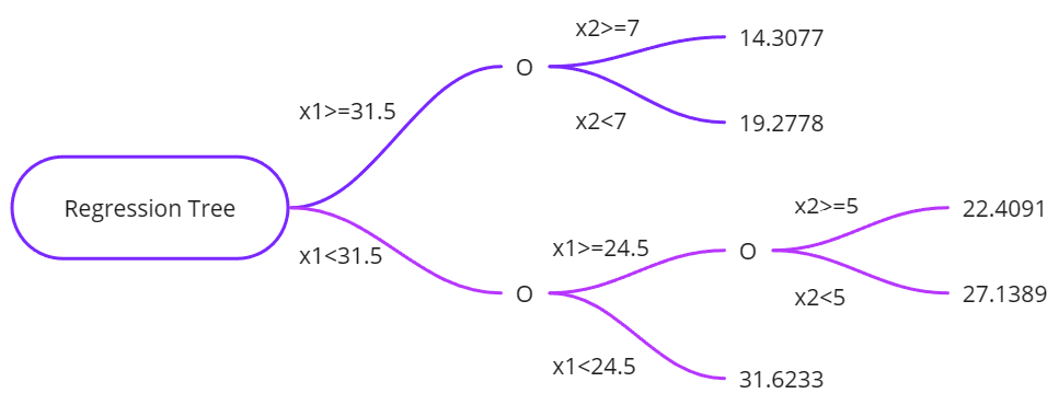
Figure 1: Regression Tree.

Regression is used in various domains, including finance, healthcare, social sciences, sports, and engineering. Some practical applications include house price prediction [19], energy consumption forecasting [20], healthcare and disease prediction [21], stock price forecasting [22], and customer lifetime value prediction [23].

In the following subsections, we will review the most common lost functions and performance metrics used for regression.

3.1 Regression Loss Functions

Table 2 shows the common loss functions used for regression and their applications.

The following subsections describe each of these loss functions in more detail.

Table 2: Loss Functions and their applications in regression tasks.

Loss Function	Applications
Mean Squared Error (MSE)	Linear Regression, Ridge Regression, Lasso Regression, Neural Networks, Support Vector Regression, Decision Trees, Random Forests, Gradient Boosting
Mean Absolute Error (MAE)	Quantile Regression, Robust Regression, L1 Regression, Neural Networks, Decision Trees, Random Forests, Gradient Boosting
Huber Loss	Robust Linear Regression, Robust Neural Networks, Gradient Boosting, Random Forests
Log-Cosh Loss	Robust Regression, Neural Networks, Gradient Boosting
Quantile Loss	Quantile Regression, Distributional Regression, Extreme Value Prediction
Poisson Loss	Poisson Regression, Count Data Prediction, Generalized Linear Models, Neural Networks, Gradient Boosting

3.1.1 Mean Squared Error (MSE)

The Mean Square Error (MSE) measures the average of the squared differences between the predicted values and the true values [24]. The MSE loss function can be defined mathematically as

$$MSE=\frac{1}{n}\sum_{i=1}^{n}(y_{i}-\hat{y_{i}})^{2},$$ (3)

where $n$ is the number of samples, $y_{i}$ is the true value of the $i^{th}$ sample and $\hat{y_{i}}$ is the predicted value of the $i^{th}$ sample.

The MSE loss function has the following properties:

• Non-negative: Since the differences between the predicted and actual values are squared, MSE is always non-negative. A value of 0 indicates a perfect fit, while larger values correspond to higher discrepancies between predictions and actual values.

• Quadratic: MSE is a quadratic function of the prediction errors, which means it places more emphasis on larger errors than smaller ones. This property makes it sensitive to outliers and can lead to models that prioritize reducing large errors over smaller ones.

• Differentiable: MSE is a smooth and continuous function for the model parameters. This property allows for the efficient computation of gradients, which is essential for optimization algorithms like gradient descent.

• Convex: MSE is a convex function, which means it has a unique global minimum. This property simplifies the optimization process, as gradient-based optimization techniques can converge to the global minimum without getting trapped in local minima. However, for deep neural networks, the error landscape is generally non-convex due to the multiple layers of non-linear activation functions, leading to a complex and highly non-linear optimization problem.

• Scale-dependent: The value of MSE depends on the scale of the target variable, making it difficult to compare the performance of models across different problems or target variable scales. For this purpose, researchers often use the root mean squared error (RMSE) or mean squared percentage error (MSPE).

The MSE, also called L2 loss, is computationally simple. However, it is not robust to outliers due to the square of the error term. Thus if the data includes outliers, it is better to use another loss function, such as Mean Absolute Error (MAE) which is more robust to outliers, or Huber Loss, which is a combination of MSE and MAE. The MSE is also used as a performance metric.

3.1.2 Mean Absolute Error (MAE)

The Mean Absolute Error (MAE) is another commonly used loss function in regression problems. It measures the average of the absolute differences between the predicted values and the true values [25]. The MAE loss can be defined as

$$MAE=\frac{1}{n}\sum_{i=1}^{n}|y_{i}-\hat{y_{i}}|,$$ (4)

where $n$ is the number of samples, $y_{i}$ and $\hat{y_{i}}$ are the true and predicted value of the $i^{th}$ sample.

The MAE loss function has the following properties:

• Non-negative: Like MSE, MAE is always non-negative because it takes the absolute value of the differences between predicted and actual values. A value of 0 indicates a perfect fit, while larger values correspond to higher discrepancies between predictions and actual values.

• Linear: MAE is a linear function of the prediction errors, which treats all errors equally regardless of their magnitude. This property makes MAE less sensitive to outliers than MSE, as it does not disproportionately emphasize large errors.

• Robust: Due to its linear nature and reduced sensitivity to outliers, MAE is considered a more robust loss function than MSE. This makes it suitable for applications where the presence of outliers is expected or the distribution of errors is not symmetric.

• Non-differentiable: Although MAE is continuous, it is not differentiable when the prediction error is zero due to the absolute value function. This property can complicate the optimization process for specific algorithms, particularly those relying on gradient-based techniques. However, subgradient methods[26, 27, 28, 29] can be employed to overcome this issue.

• Convex: MAE is a convex function, which means it has a unique global minimum. This property simplifies the optimization process, as gradient-based optimization techniques can converge to the global minimum without getting trapped in local minima. Like the MSE, the MAE is non-convex for Deep neural networks due to the multiple layers with non-linear activation functions.

• Scale-dependent: Like MSE, the value of MAE depends on the scale of the target variable, making it difficult to compare the performance of models across different problems or target variable scales. To address this issue, researchers often use scale-invariant metrics such as mean absolute percentage error (MAPE) or normalized mean absolute error (NMAE) to compare models across different scales or units.

The MAE, called L1 loss, is often used as an evaluation metric. It is computationally simple and easy to understand, but it does not have the smooth and differentiable property of the MSE and is not sensitive to outliers.

3.1.3 Huber Loss

The Huber loss combines the properties of both Mean Squared Error (MSE) and Mean Absolute Error (MAE). Huber loss is designed to be more robust to outliers than MSE while maintaining smoothness and differentiability [30]. The Huber loss function is defined as

$$L(y,\hat{y})=\begin{cases}\frac{1}{2}(y-\hat{y})^{2}&\text{for }|y-\hat{y}|\leq\delta\\ \delta(|y-\hat{y}|-\frac{1}{2}\delta)&\text{otherwise},\end{cases}$$ (5)

where $y$ is the true value, $\hat{y}$ is the predicted value, and $\delta$ is a user-specified threshold value.

When the error is small, the Huber loss function behaves like the MSE loss function, and when the error is large, the Huber loss function behaves like the MAE loss function. This property makes the Huber loss function more robust to outliers than the MSE loss function, as it is less sensitive to large errors.

The Huber loss function is differentiable, which makes it suitable for use in gradient-based optimization algorithms such as stochastic gradient descent (SGD). It is commonly used in linear regression and time series forecasting, as it can handle outliers and noise in the data. It is also used in robust optimization problems where the data may contain outliers or noise.

The threshold $\delta$ can be chosen empirically by trying different values and evaluating the model’s performance. However, common practice is to set $\delta$ to a small value if the data has a lot of noise and to a large value if the data has outliers.

3.1.4 Log-Cosh Loss

The Log-Cosh loss function is smooth and differentiable. It is commonly used in regression problems where the data may contain outliers or noise [31]. The Log-Cosh loss is defined as

$$L(y,\hat{y})=\frac{1}{n}\sum_{i=1}^{n}\log(\cosh(y_{i}-\hat{y}_{i})),$$ (6)

where $y$ is the true value, $\hat{y}$ is the predicted value and $n$ is the number of samples.

One of the advantages of the log-cosh loss function is that it is less sensitive to outliers than the mean squared error (MSE), as it is not affected by extreme data values. However, it is more sensitive to small errors than the Huber loss.

3.1.5 Quantile Loss

Also known as quantile regression loss, this function is often used for predicting an interval instead of a single value [32]. If we denote the quantile as $q$ where $0<q<1$, and the predicted and actual values as $\hat{y}$ and $y$ respectively, then the quantile loss is given by

$$L(y,\hat{y})=q\cdot\max(y-\hat{y},0)+(1-q)\cdot\max(\hat{y}-y,0)$$ (7)

$\max(a,b)$ represents the maximum of $a$ and $b$. The expression $y-\hat{y}$ is used when the prediction underestimates, and $\hat{y}-y$ is used when the prediction overestimates. The loss is scaled by $q$ for underestimations and $(1-q)$ for overestimations.

Note that when $q=0.5$, the quantile loss is equivalent to the Mean Absolute Error (MAE), making it a generalization of MAE that allows for asymmetric penalties for underestimations and overestimations.

Overestimation occurs when a model’s prediction exceeds the actual value. Underestimation is the opposite of overestimation. It occurs when a model’s prediction is lower than the actual value.

Practical examples of quantile regression include:

Financial Risk Management: To estimate Value-at-Risk (VaR) and Conditional Value-at-Risk (CVaR), which are measures of financial risk used in risk management. These quantile-based measures help to understand the potential for extreme losses [33].

Supply Chain and Inventory Management: Predicting demand for products can benefit from quantile loss as it can give a range of potential demand rather than a single point, which can help manage inventory and reduce stockouts or overstock situations [34].

Energy Production: To predict power output, having a range of potential outputs to manage grid stability [35].

Economic Forecasting: Predicting economic indicators can use quantile regression to give a range of possible values, which can help planning and policy-making [36].

Weather Forecasting: Can be useful for predicting variables like temperature or rainfall, where providing a range can be more informative than a single-point estimate [37, 38].

Real Estate Pricing: Predicting the price of a property within a range can be more useful than predicting a single price [39].

Healthcare: Quantile regression can predict a range of possible patient outcomes based on a set of features, which can assist doctors in making more informed decisions [40].

3.1.6 Poisson Loss

Poisson loss is used in regression tasks when the target variable represents count data and is assumed to follow a Poisson distribution. The Poisson loss is derived from the negative log-likelihood of the Poisson distribution. It maximizes the likelihood of observing the count data given the predicted values [41]. It s defined as

$$L(y,\hat{y})=\frac{1}{n}\sum_{i=1}^{n}(\hat{y}_{i}-y_{i}\log(\hat{y}_{i})),$$ (8)

where $y_{i}$ represents the actual target value, $\hat{y}_{i}$ is the predicted value, and $n$ is the number of samples.

When applying the Poisson loss function to model count data, we must ensure that the predicted values are non-negative since negative counts are not meaningful in real-world scenarios. To achieve this, it is common to use a link function that transforms the linear combination of input features to a non-negative output, which can then be interpreted as the expected count.

A link function is a mapping from the linear predictor to the predicted value. In the context of Poisson regression, the exponential function is a common choice for the link function because it guarantees non-negative outputs. The exponential function has the following form:

$$\hat{y}_{i}=\exp(\mathbf{w}^{\top}\mathbf{x}_{i}+b),$$ (9)

where $\mathbf{w}$ is a vector of weights, $\mathbf{x}_{i}$ is a vector of input features for the $i$-th observation, and $b$ is the bias term.

Using the exponential function as a link function, we ensure that the predicted values $\hat{y}_{i}$ are always non-negative. In this case, the Poisson loss function can be written as

$$L(y,\hat{y})=\frac{1}{n}\sum_{i=1}^{n}\left(\exp(\mathbf{w}^{\top}\mathbf{x}_{i}+b)-y_{i}\log(\exp(\mathbf{w}^{\top}\mathbf{x}_{i}+b))\right)$$ (10)

The Poisson distribution is typically used for modeling the number of times an event occurred in an interval. Here are some examples of applications where Poisson loss can be useful.

Traffic Modeling: Poisson regression can predict the number of cars that pass through a toll booth during a given time interval based on factors like the time of day, day of the week, and weather conditions [42].

Healthcare: Epidemiology can predict the number of disease cases in different regions based on variables like population density, vaccination rates, and social behavior patterns [43].

Insurance: In the insurance industry, it can be used to model claim counts for certain types of insurance policies [44].

Customer Service: Poisson regression can be used to predict the number of calls that a call center receives during different times of the day, to aid in staff scheduling [45].

Internet Usage: It can be used to model the number of website visits or clicks on an ad during a given time interval to help understand user behavior and optimize ad placement [46].

Manufacturing: It can predict the number of defects or failures in a manufacturing process, helping in quality control and maintenance planning [47].

Crime Analysis: Poisson regression can be used to model the number of occurrences of certain types of crimes in different areas to help in police resource allocation and crime prevention strategies [48].

3.2 Regression Performance Metrics

Table 3 shows the most common metrics used in regression tasks. The following sections delve into more details on each of these metrics skipping the mean square error (MSE) and the mean absolute error (MAE) because they are the same discussed previously as loss functions.

Table 3: Common performance metrics used in regression.

Performance Metric	Applications
Mean Squared Error (MSE)	General-purpose regression, model selection,
	optimization, linear regression, neural networks
Root Mean Squared Error (RMSE)	General-purpose regression, model selection,
	optimization, linear regression, neural networks
Mean Absolute Error (MAE)	General-purpose regression, model selection,
	optimization, robustness to outliers,
	time series analysis
R-squared (R²)	Model evaluation, goodness-of-fit, linear regression,
	multiple regression
Adjusted R-squared	Model evaluation, goodness-of-fit, linear regression,
	multiple regression with many predictors
Mean Squared Logarithmic Error	Forecasting, model evaluation, skewed
(MSLE)	target distributions, finance, sales prediction
Mean Absolute Percentage Error	Forecasting, model evaluation, time series analysis,
(MAPE)	business analytics, supply chain optimization

3.2.1 Root Mean Squared Error (RMSE)

The Root Mean Square Error (RMSE) is the square root of the mean squared error (MSE) defined as

$$RMSE=\sqrt{\frac{1}{n}\sum_{i=1}^{n}(y_{i}-\hat{y}_{i})^{2}},$$ (11)

where $y_{i}$ is the true value, $\hat{y}_{i}$ is the predicted value, and $n$ is the number of samples.

The RMSE measures the average deviation of the predictions from the true values. This metric is easy to interpret because it is in the same units as the data. However, it is sensitive to outliers. Lower RMSE values indicate better model performance, representing smaller differences between predicted and actual values.

3.2.2 Mean Absolute Percentage Error (MAPE)

The Mean Absolute Percentage Error (MAPE) measures the average percentage error of the model’s predictions compared to the true values. It is defined as

$$MAPE=\frac{1}{n}\sum_{i=1}^{n}\frac{|y_{i}-\hat{y}_{i}|}{y_{i}}\times 100,$$ (12)

where $y_{i}$ is the true value, $\hat{y}_{i}$ is the predicted value, and $n$ is the number of samples.

One of the advantages of using MAPE is that it is easy to interpret, as it is expressed in percentage terms. It is also scale-independent, which can be used to compare models across different scales of the target variable. However, it has two limitations: it can produce undefined results when $y_{i}$ is zero and is sensitive to outliers.

3.2.3 Symmetric Mean Absolute Percentage Error (SMAPE)

The Symmetric Mean Absolute Percentage Error (SMAPE) is a variation of the Mean Absolute Percentage Error (MAPE) commonly used to evaluate the accuracy of predictions in time series forecasting [49]. SMAPE is defined as

$$SMAPE=\frac{2}{n}\sum_{i=1}^{n}\frac{|y_{i}-\hat{y}_{i}|}{|y_{i}|+|\hat{y}_{i}|}*100,$$ (13)

where $y_{i}$ is the true value, $\hat{y}_{i}$ is the predicted value, and $n$ is the number of samples.

One of the advantages of using SMAPE is that it is symmetric, which means that it gives equal weight to over-predictions and under-predictions. This is particularly useful when working with time series data, where over-predictions and under-predictions may have different implications, and SMAPE helps to ensure that the model is equally penalized for both types of errors, leading to better overall performance in terms of how well it meets the business needs or objectives. However, SMAPE has some limitations; for example, it can produce undefined results when both $y_{i}$ and $\hat{y}_{i}$ are zero and can be sensitive to outliers.

The implications of over-predictions and under-predictions varied depending on the application. In the following, we discuss real-world examples.

Inventory Management: Over-predicting demand can lead to excess inventory, which ties up capital and can result in waste if products expire or become obsolete. Under-predicting demand can lead to stockouts, lost sales, and damage to customer relationships [50]. A symmetric error measure like SMAPE penalizes both cases because over-prediction and under-prediction have costly implications.

Energy Demand Forecasting: Over-prediction of energy demand can cause unnecessary production, leading to waste and increased costs. Under-prediction can lead to insufficient power generation, resulting in blackouts or the need for expensive on-demand power generation [51].

Financial Markets: In financial markets, over-prediction of a stock price might lead to unwarranted investments resulting in financial loss, while under-prediction might result in missed opportunities for gains [52].

Sales Forecasting: Over-prediction of sales could lead to overstaffing, overproduction, and increased costs, while under-prediction could lead to understaffing, missed sales opportunities, and decreased customer satisfaction [53].

Transportation and Logistics: Over-predicting the demand for transportation might lead to underutilized vehicles or routes, resulting in unnecessary costs. Under-predicting demand might lead to overcrowding and customer dissatisfaction [54].

3.2.4 Coefficient of Determination $R^{2}$

The Coefficient of Determination ($R^{2}$), measures how well the model can explain the variation in the target variable [55]. $R^{2}$ is defined as the proportion of the variance in the target variable that the model explains. It ranges from 0 to 1, where 0 means that the model does not explain any variation in the target variable, and one means that the model explains all the variation in the target variable.

The formula for R-squared is

$$R^{2}=1-\frac{\sum_{i=1}^{n}(y_{i}-\hat{y}i)^{2}}{\sum{i=1}^{n}(y_{i}-\bar{y})^{2}},$$ (14)

where $y_{i}$ is the true value, $\hat{y}_{i}$ is the predicted value, $\bar{y}$ is the mean of the true values, and $n$ is the number of samples.

Benefits and Limitations of R-squared

Some of the main benefits of $R^{2}$ are:

1. Measures the relationship between the model and the response variable: R-squared describes the strength of the relationship between the model and the response variable on a convenient 0 – 1 scale.

2. Interpretable: It can be more interpretable than other statistics because it provides a percentage that can be intuitively understood.

3. Helps in model selection: If we have two models, we can compare their R-squared values as a part of the selection process. The model with the higher R-squared could indicate a better fit.

The limitations of $R^{2}$ include:

1. Misleading with non-linear relationships: $R^{2}$ works as intended in a simple linear regression model with one explanatory variable but can be misleading with more complex, nonlinear, or multiple regression models.

2. Influenced by the number of predictors: $R^{2}$ always increases as we add more predictors to a model, even if they are unrelated to the outcome variable. This can lead to overly complex models that overfit the data. This is the benefit of the adjusted $R^{2}$, which adjusts the $R^{2}$ value based on the number of predictors in the model.

3. Sensitive to outliers: $R^{2}$ is sensitive to outliers.

4. Does not check for biased predictions: $R^{2}$ cannot determine whether the coefficient estimates and predictions are biased, which is to say, whether the predictions systematically over or underestimate the actual values.

5. Limitation with small sample sizes: When the sample size is small, the $R^{2}$ value might be unreliable. It can be artificially high or low and might not represent the true strength of the relationship between the variables.

3.2.5 Adjusted $R^{2}$

Adjusted $R^{2}$ is a modified version of $R^{2}$ that has been adjusted for the number of predictors in the model. It increases only if the new term improves the model more than would be expected by chance. It decreases when a predictor improves the model by less than expected by chance [56]. The adjusted R-squared is defined as

$$\text{Adjusted }R^{2}=1-\left(\frac{(1-R^{2})(n-1)}{n-k-1}\right),$$ (15)

where $n$ is the number of observations, $k$ is the number of predictors. The adjustment is a penalty for adding unnecessary predictors to the model. This penalty increases with the increase in the number of predictors. This is particularly useful in multiple regression, where several predictors are used simultaneously.

The Adjusted $R^{2}$ is often used for model comparison, as it won’t necessarily increase with adding more variables to the model, unlike regular $R^{2}$. It is useful when we need to compare models of different sizes. Unlike $R^{2}$, its value can be negative, meaning that the model is a poor fit for the data.

4 Classification

Classification is a supervised machine learning task in which a model is trained to predict the class or category of a given input data point. Classification aims to learn a mapping from input features to a specific class or category.

There are different classification tasks, such as binary classification, multi-class classification, and multi-label classification. Binary classification is a task where the model is trained to predict one of two classes, such as "spam" or "not spam," for an email. Multi-class classification is a task where the model is trained to predict one of the multiple classes, such as "dog," "cat," and "bird," for an image. Multi-label classification is a task where the model is trained to predict multiple labels for a single data point, such as "dog" and "outdoor," for an image of a dog in the park.

Classification algorithms can be based on techniques such as decision trees, Naive Bayes, k-nearest neighbors, Support Vector Machines, Random Forest, Gradient Boosting, Neural Networks, and others.

4.1 Classification Loss Functions

Several loss functions can be used for classification tasks, depending on the specific problem and algorithm. In the following sections, we describe the most common loss functions used for classification:

4.1.1 Binary Cross-Entropy Loss (BCE)

The Binary Cross Entropy (BCE), also known as log loss, is a commonly used loss function for binary classification problems. It measures the dissimilarity between the predicted probability of a class and the true class label [57]. Cross-entropy is a well-known concept in information theory commonly used to measure the dissimilarity between two probability distributions. In binary classification, the true class is usually represented by a one-hot encoded vector, where the true class has a value of 1, and the other class has a value of 0. The predicted probability is represented by a vector of predicted probabilities for each class, where the predicted probability of the true class is denoted by $p(y=1|x)$ and the predicted probability of the other class is denoted by $p(y=0|x)$.

The loss function is defined as

$$L(y,p)=-(y\log(p)+(1-y)\log(1-p))$$ (16)

Which intuitively can be split into two parts:

$$\begin{cases}-log(p)&\text{if }y=1\\ -log(1-p)&\text{if }y=0,\end{cases}$$ (17)

where $y$ is the true class label (0 or 1) and $p$ is the predicted probability of the positive class. The loss function is minimized when the predicted probability $p$ equals the true class label $y$.

The binary cross-entropy loss has several desirable properties, such as being easy to compute, differentiable, and providing a probabilistic interpretation of the model’s output. It also provides a smooth optimization surface and is less sensitive to outliers than other loss functions. However, it is sensitive to the class imbalance problem, which occurs when the number of samples of one class is significantly greater than the other. We can use the Weighted Binary Cross Entropy for these cases.

4.1.2 Weighted Binary Cross Entropy (WBCE)

Variation of the standard binary cross-entropy loss function, where the weight of each sample is considered during the loss calculation. This is useful in situations where the distribution of the samples is imbalanced [58].

In the standard binary cross-entropy loss, the loss is calculated as the negative log-likelihood of the true labels given the predicted probabilities. In the Weighted Binary Cross Entropy (WBCE), a weight is assigned to each sample, and the loss for each sample is calculated as

$$L=-(w_{i}\cdot ylog(p)+w_{i}(1-y)log(1-p)),$$ (18)

where $w_{i}$ is the weight assigned to the $i^{th}$ sample, $y$ is the true label, and $p$ is the predicted probability of the positive class.

By assigning a higher weight to samples from under-represented classes, the model is encouraged to pay more attention to these samples, and the model’s overall performance can be improved.

4.1.3 Categorical Cross-entropy Loss (CCE)

The Categorical Cross Entropy (CCE), also known as the negative log-likelihood loss or Multi-class log loss, is a function used for multi-class classification tasks. It measures the dissimilarity between the predicted probability distribution and the true distribution [59].

Given the predicted probability distribution, it is defined as the average negative log-likelihood of the true class. The formula for categorical cross-entropy loss is expressed as

$$L=-\frac{1}{N}\sum_{i=1}^{N}\sum_{j=1}^{C}y_{i,j}log(p_{i,j}),$$ (19)

where $N$ is the number of samples, $C$ is the number of classes, $y$ is the true label, and $p$ is the predicted probability of the true class. The loss is calculated for each sample and averaged over the entire dataset.

The true label is a one-hot encoded vector in traditional categorical cross-entropy loss, where the element corresponding to the true class is one, and all other elements are 0. However, in some cases, it is more convenient to represent the true class as an integer, where the integer value corresponds to the index of the true class leading to the sparse categorical cross-entropy loss discussed next.

4.1.4 Sparse Categorical Cross-entropy Loss

Variation of the categorical cross-entropy loss used for multi-class classification tasks where the classes are encoded as integers rather than one-hot encoded vectors [59]. Given that the true labels are provided as integers, we directly select the correct class using the provided label index instead of summing over all possible classes. Thus the loss for each example is calculated as

$$H(y,\hat{y})=-\log(\hat{y}_{i,y_{i}})$$ (20)

And the final sparse categorical cross-entropy loss is the average over all the samples:

$$H(Y,\hat{Y})=-\frac{1}{n}\sum_{i=1}^{n}\log(\hat{y}_{i,y_{i}}),$$ (21)

where $y_{i}$ is the true class of the $i$-th sample and $\hat{y}_{i,y_{i}}$ is the predicted probability of the $i$-th sample for the correct class $y_{i}$.

4.1.5 Cross-Entropy loss with label smoothing

In the Cross-Entropy loss with label smoothing, the labels are smoothed by adding a small value to the true label and subtracting the same value from all other labels. This helps reduce the model’s overconfidence by encouraging it to produce more uncertain predictions [60, 61].

The motivation behind this is that when training a model, it is common to become over-confident in its predictions, particularly when trained on a large amount of data. This overconfidence can lead to poor performance on unseen data. Label smoothing helps to mitigate this problem by encouraging the model to make less confident predictions.

The formula for the Cross-Entropy loss with label smoothing is similar to the standard categorical cross-entropy loss but with a small epsilon added to the true label and subtracted from all other labels. The formula is given by

$$L(y,\hat{y})=-\sum_{c=1}^{C}\left[(1-\epsilon)y_{c}\log\hat{y}_{c}+\frac{\epsilon}{C}\log\hat{y}_{c}\right],$$ (22)

where $y$ is the true label, $\hat{y}$ is the predicted label, $C$ is the number of classes, and $\epsilon$ is the smoothing value. Typically, $\epsilon$ is set to a small value, such as 0.1 or 0.2.

Label smoothing does not always improve performance, and it is common to experiment with different epsilon values to find the best value for a specific task and dataset.

4.1.6 Focal loss

The focal loss introduced by Tsung-Yi Lin et al. [62] is a variation of the standard cross-entropy loss that addresses the issue of class imbalance, which occurs when the number of positive samples (objects of interest) is much smaller than the number of negative samples (background). In such cases, the model tends to focus on the negative samples and neglect the positive samples, leading to poor performance. The focal loss addresses this issue by down-weighting the easy negative samples and up-weighting the hard positive samples.

The focal loss is defined as

$$FL(p_{t})=-\alpha_{t}(1-p_{t})^{\gamma}log(p_{t}),$$ (23)

where $p_{t}$ is the predicted probability for the true class, $\alpha_{t}$ is a weighting factor that controls the importance of each example, and $\gamma$ is a focusing parameter that controls the rate at which easy examples are down-weighted.

The weighting factor $\alpha_{t}$ is usually set to the inverse class frequency to balance the loss across all classes. The focusing parameter $\gamma$ is typically set to a value between 2 and 4 to give more weight to hard examples.

In the original paper, the authors used a sigmoid activation function for binary classification and the cross-entropy loss for multi-class classification. The focal loss is combined with these loss functions to improve the performance of object detection and semantic segmentation models.

In recent works, focal loss has been used in object detection, semantic [63], instance segmentation [64], and human pose estimation [65].

4.1.7 Hinge Loss

Hinge loss is a popular function used for maximum-margin classification, commonly used for support vector machines (SVMs) for example in one-vs-all classification where we classify an instance as belonging to one of many categories and situations where we want to provide a margin of error [66].

The hinge loss function for an individual instance can be represented as

$$L(y,f(x))=\max(0,1-y\cdot f(x)),$$ (24)

where $y$ is the true label of the instance, which should be -1 or 1 in a binary classification problem. $f(x)$ is the predicted output for the instance $x$. The raw margin is $y\cdot f(x)$.

The hinge loss is 0 if the instance is on the correct side of the margin. The loss is proportional to the distance from the margin for data on the wrong side of the margin.

4.2 Classification Performance Metrics

Table 4 summarizes the common metrics used for classification. The following sections will delve into each of these metrics.

Table 4: Metrics used in classification task.

Common Name	Other Names	Abbr	Definitions	Interpretations
True Positive	Hit	TP	True Sample	Correctly labeled
			labeled true	True Sample
True Negative	Rejection	TN	False Sample	Correctly labeled
			labeled false	False sample
False Positive	False alarm	FP	False sample	Incorrectly labeled
	Type I Error		labeled True	False sample
False Negative	Miss,	FN	True sample	Incorrectly label
	Type II Error		labeled false	True sample
Recall	True Positive	TPR	TP/(TP+FN)	$\%$ of True samples
	Rate			correctly labeled
Specificity	True Negative	SPC,	TN/(TN+FP)	$\%$ of False samples
	Rate	TNR		correctly labeled
Precision	Positive Pre-	PPV	TP/(TP+FP)	$\%$ of samples labeled
	dictive Value			True that really are True
Negative Predi-		NPV	TN/(TN+FN)	$\%$ of samples labeled
ctive Value				False that really are False
False Negative		FNR	FN/(TP+FN)=	$\%$ of True samples
Rate			1-TPR	incorrectly labeled
False Positive	Fall-out	FPR	FP/(FP+FN)=	$\%$ of False samples
Rate			1-SPC	incorrectly labeled
False Discovery		FDR	FP/(TP+FP)=	$\%$ of samples labeled
Rate			1-PPV	True that are really False
True Discovery		TDR	FN/(TN+FN)=	$\%$ of samples labeled
Rate			1-NPV	False that are really True
Accuracy		ACC	$\frac{(TP+TN)}{(TP+TN+FP+FN)}$	Percent of samples
				correctly labeled
F1 Score		F1	$\frac{(2*TP)}{((2*TP)+FP+FN)}$	Approaches 1 as
				errors decline

4.2.1 Confusion Matrix

The confusion matrix is used to define a classification algorithm’s performance. It contains the number of true positives (TP), true negatives (TN), false positives (FP), and false negatives (FN) that result from the algorithm. The confusion matrix for a binary classification problem is represented in a 2x2 table as shown in Table 5.

Table 5: Confusion Matrix

	Predicted Positive	Predicted Negative
Actual Positive	True Positive (TP)	False Negative (FN)
Actual Negative	False Positive (FP)	True Negative (TN)

For example, consider a binary classification problem where the algorithm tries to predict whether an image contains a cat. The confusion matrix for this problem would look like Table 6:

Table 6: Confusion Matrix

	Predicted as Cat	Predicted as Not Cat
Actual Cat	TP	FN
Actual Not Cat	FP	TN

Where:

• TP: the number of images correctly classified as cats.

• TN: the number of images correctly classified as not cats.

• FP: the number of images incorrectly classified as cats.

• FN: the number of images incorrectly classified as not cats.

Using the values in the confusion matrix, we can calculate performance metrics such as accuracy, precision, recall, and F1-score.

4.2.2 Accuracy

Accuracy is a commonly used metric for object classification. It is the ratio of correctly classified samples to the total number of samples [67]. Mathematically, it can be represented as

$$Accuracy=\frac{Number\ of\ Correctly\ Classified\ Samples}{Total\ Number\ of\ Samples}$$ (25)

Accuracy can be expressed in terms of the confusion matrix values as

$$Accuracy=\frac{TP+TN}{TP+FP+TN+FN}$$ (26)

It is a simple and intuitive metric, but it can be misleading when the class distribution is imbalanced, as it tends to favor the majority class. For example, let’s assume that we want to predict the presence of cancer in a cell. If for every 100 samples, only one contains cancer, a useless model that always predicts "No cancer" will have an accuracy of 99%. Other metrics, such as precision, recall, or F1-score, are more appropriate in these cases.

4.2.3 Precision

Precision measures the accuracy of positive predictions. It is defined as the number of true positive predictions divided by the number of true positive predictions plus the number of false positive predictions [68]. Mathematically, it can be represented as

$$Precision=\frac{TP}{TP+FP},$$ (27)

where $TP$ is the number of true positive predictions, and $FP$ is the number of false positive predictions.

Precision is useful when the cost of a false positive prediction is high, such as in medical diagnosis or fraud detection. A high precision means the model is not generating many false positives, so the predictions are reliable. However, it is important to note that precision is not the only metric to consider when evaluating a model’s performance, as high precision can also be achieved by a model that is not generating many positive predictions at all, which would result in a low recall.

4.2.4 Recall, Sensitivity, or True Positive Rate (TPR)

The recall metric, also known as sensitivity or True Positive Rate (TPR), measures the proportion of true positive instances (i.e., instances correctly classified as positive) out of the total number of positive instances [68]. Mathematically, it is represented as

$$Recall=\frac{TruePositives}{TruePositives+FalseNegatives}$$ (28)

It measures how well the model can identify all the positive instances in the dataset. A high recall value indicates the model has fewer false negatives, meaning it can correctly identify the most positive instances. However, a high recall value does not necessarily mean the model has a high precision, as the number of false positives can also influence it.

4.2.5 Precision-Recall Tradeoff

The precision-recall tradeoff refers to the inverse relationship between precision and recall. As one metric increases, the other tends to decrease.

Imagine a machine learning model trying to predict whether an email is spam. If the model is tuned to be very conservative and only marks an email as spam when confident, it is likely to have high precision (i.e., if it marks an email as spam, it is very likely to be spam). However, this conservative approach means it will probably miss many spam emails it is unsure about, leading to a lower recall.

Conversely, if the model is tuned to be liberal and marks emails as spam more freely, it will probably identify most spam emails correctly, leading to a high recall. However, this approach will also incorrectly mark many non-spam emails as spam, leading to a lower precision.

This tug-of-war between precision and recall is the crux of the tradeoff. An optimal balance between the two must be found depending on the use case. For instance, in a medical context, a high recall might be prioritized to ensure that all possible disease cases are identified, even at the expense of some false positives. On the other hand, a spam detection system might aim for high precision to avoid annoying users with wrongly classified emails, accepting that some spam messages might slip through.

The precision-recall tradeoff is a crucial consideration when tuning machine learning models. Maximizing both metrics is only sometimes possible; thus, a balance must be struck based on the requirements and constraints of the specific application.

4.2.6 F1-score

The F1 score combines precision and recall to provide a single value representing a classification model’s overall performance [68]. It is defined as the harmonic mean of precision and recall computed as

$$F1=2*\frac{precision\cdot recall}{precision+recall}$$ (29)

The F1 score considers both the model’s ability to correctly identify positive examples (precision) and the ability of the model to identify all positive examples in the dataset (recall). A higher F1 score indicates that the model has a better balance of precision and recall, whereas a low F1 score indicates that the model may have a high precision or recall but not both.

It is particularly useful when the class distribution is imbalanced, or we want to give equal weight to precision and recall.

4.2.7 F2-score

The F2 score is a variation of the F1 score, with more weight given to the recall metric. The F2 score is the harmonic mean of precision and recall, with a weighting factor of 2 for recall [68]. The formula for the F2 score is

$$F2=(1+2^{2})\frac{Precision*Recall}{2^{2}*Precision+Recall}$$ (30)

Like the F1 score, the F2 score ranges from 0 to 1, with a higher score indicating better performance. However, the F2 score places a greater emphasis on recall, making it useful when it is important to minimize false negatives. For example, a false negative could mean a patient is not diagnosed with a serious disease in medical diagnosis, so the F2 score is often used in such scenarios [69].

4.2.8 Specificity

Specificity, also known as the true negative rate (TNR), is a metric that measures the proportion of actual negatives that are correctly identified as negatives by a classification model. It is defined as the number of true negatives (TN) divided by the number of true negatives plus the number of false positives (FP) [70]. The formula for specificity is

$$Specificity=\frac{TN}{TN+FP}$$ (31)

This metric is particularly useful in medical diagnostic testing, where it is important to minimize the number of false positives to avoid unnecessary treatments or interventions. High specificity indicates that the model is good at identifying negatives and has a low rate of false positives.

It is often used with the Recall or TPR to evaluate the overall performance of a classification model.

4.2.9 False Positive Rate (FPR)

The False Positive Rate (FPR) is used to evaluate the proportion of false positives (i.e., instances that are incorrectly classified as positive) to the total number of negatives (i.e., instances that are correctly classified as negative). It is also known as the Type I Error rate, which complements the Specificity metric.

Formally, the FPR is calculated as

$$FPR=\frac{FP}{FP+TN}$$ (32)

FPR directly relates to the threshold classifying instances as positive or negative. A lower threshold will increase the number of false positives and thus increase the FPR, while a higher threshold will decrease the number of false positives and decrease the FPR.

In practice, the FPR is often plotted on the x-axis of a Receiver Operating Characteristic (ROC) curve to visualize the trade-off between the TPR and FPR for different classification thresholds. See section 4.2.14 for more details.

4.2.10 Negative Predictive Value (NPV)

The Negative Predictive Value (NPV) measures the proportion of negative cases that are correctly identified as such [70]. It is calculated as

$$NPV=\frac{TN}{TN+FN}$$ (33)

The NPV is useful when the cost of a false negative (i.e., an actual negative case being classified as positive) is high. For example, a false negative result in medical diagnostics can delay treatment or even death. In such cases, a high NPV is desired.

The NPV is not affected by the prevalence of the condition in the population, whereas other metrics, such as sensitivity and specificity, are. This makes the NPV a useful metric for evaluating the performance of a classifier when the class distribution is imbalanced.

The NPV can be interpreted as the complement of the false positive rate (FPR)

$$NPV=1-FPR$$ (34)

4.2.11 True Discovery Rate (TDR)

True Discovery Rate (TDR) evaluates the proportion of true positive predictions a model makes among all the positive predictions. It is also known as the Positive Predictive Value (PPV) or precision of the positive class [70]. TDR is calculated as

$$TDR=\frac{TP}{TP+FP}$$ (35)

TDR is a useful metric for evaluating the performance of a model in situations where the number of false positive predictions is high, and the number of true positive predictions is low. It is particularly useful in high-dimensional datasets where the number of features is large and the number of positive observations is low. TDR can provide a more accurate picture of the model’s performance than accuracy or recall in such cases.

There may be a trade-off between TDR and recall in some cases: TDR may be low when the recall is high, and vice versa. Therefore, it’s important to consider both TDR and recall when evaluating the performance of a model.

4.2.12 False Discovery Rate (FDR)

The False Discovery Rate (FDR) measures the proportion of false positives among all positive predictions made by a classifier [70]. It is defined as

$$FDR=\frac{FP}{TP+FP}$$ (36)

The FDR can be an alternative to the False Positive Rate (FPR) when the cost of false positives and true negatives differs. It is particularly useful in cases where the number of false positives is more critical than the number of false negatives, such as in medical testing or fraud detection. A lower FDR value indicates that the classifier makes fewer false positive predictions.

4.2.13 Precision-Recall Curve

The precision-recall (PR) curve is a graphical representation of the trade-off between precision and recall for different threshold values of a classifier. Precision is the proportion of true positive predictions out of all positive predictions, while recall is the proportion of true positive predictions out of all actual positive instances. The precision-recall curve plots precision on the y-axis and recall on the x-axis for different threshold values of the classifier [68].

Computing the Precision-Recall Curve

1. Start with a binary classifier that can predict a binary outcome and estimate the probability of the positive class. These probabilities are also known as scores.

2. For every possible threshold (from 0 to 1) on these scores, calculate the Precision (see Section 4.2.3) and the Recall (see Section 4.2.4).

3. Plot a curve with Recall on the X-axis and Precision on the Y-axis. Figure 2(a) shows an example of Precision-Recall curves for three models.

Interpretation of the Precision-Recall Curve

Figure 2(a) shows the precision/recall curves for three models trained on the same data. The dashed line shows the ideal performance. Each model reports its Average Precision metric (see Section 5.2.1 for more details on Average Precision). In the following, we explain how to interpret PR curves.

The closer the curve is to the top-right corner, the better the model’s performance. Ideal performance is indicated by a point at (1,1), which signifies perfect precision (no false positives) and recall (no false negatives). If the curve is closer to the top-right corner of the plot, it indicates that the model achieves a good balance of precision and recall for most threshold settings.

The area under the curve (AUC-PR) provides a single-number summary of the information in the curve. The maximum possible AUC is 1, which corresponds to a perfect classifier. A random classifier will have an AUC of 0.5. A model with a higher AUC is generally considered better.

Steepness of the curve. Ideally, we want the recall to increase quickly as precision decreases slightly, resulting in a steep curve. This steepness reflects a good balance between precision and recall. If the curve is less steep, we are losing a lot of precision for small increases in recall.

Comparison of different models. We can compare the PR curves of different models to understand their performance. If the PR curve of one model is entirely above that of another, it indicates superior performance across all thresholds.

4.2.14 Area Under the Receiver Operating Characteristic curve (AUC-ROC)

The Area Under the Receiver Operating Characteristic Curve (AUC-ROC) is a commonly used performance metric for evaluating the performance of binary classification models [68]. It measures the ability of the model to distinguish between positive and negative classes by plotting the true positive rate (TPR) against the false positive rate (FPR) at various threshold settings. The AUC-ROC is a value between 0 and 1, with 1 indicating a perfect classifier and a value of 0.5 indicating a classifier that performs no better than random guessing.

The Area under the Receiver Operating Characteristic curve (AUC-ROC) offers a single-value summary of the model’s performance across all possible threshold values. This measure is particularly valuable when comparing the performance of different models, as its assessment is independent of threshold choice.

However, in cases where the positive and negative class distributions are significantly imbalanced, the AUC-ROC, while still applicable, may not provide the most accurate performance representation. With a heavy imbalance, the ROC curve can appear overly optimistic, as a low false positive rate can still mean a large number of false positives if the total count of actual negatives is high, resulting in a misleadingly high AUC-ROC value.

In such imbalanced scenarios, the Precision-Recall (PR) curve and its corresponding area under the curve (AUC-PR) can often provide a more nuanced and accurate performance assessment. As PR curves focus more on detecting positive instances, often the minority class in an imbalanced dataset, they can deliver a more insightful evaluation of a model’s ability to detect positive instances, providing a more relevant representation of the model’s performance.

Computing the ROC Curve

1. Start with a binary classifier that can predict a binary outcome and estimate the probability of the positive class. These probabilities are also known as scores.

2. For every possible threshold (from 0 to 1) on these scores, calculate the TPR (see Section 4.2.4) and the FPR (see Section 4.2.9).

3. Plot a curve with FPR on the X-axis and TPR on the Y-axis. Figure 2(b) shows an example of ROC curves for three models.

Interpretation of the ROC Curve

Figure 2(b) shows the ROC curves for three models trained on the same data. The dashed line shows random performance. Each model reports its Area under the curve (AUC) in the legend. In the following, we explain how to interpret ROC curves.

TPR and FPR on each axis: The True Positive Rate (TPR) is used for the vertical axis. It measures the proportion of actual positives that are correctly identified as such. The False Positive Rate (FPR), also known as the fall-out or Probability of False Alarm, measures the proportion of actual negatives that are incorrectly identified as positives. The ROC curve plots the TPR vs. FPR at different classification thresholds. Lowering the classification threshold classifies more items as positive, thus increasing both False Positives and True Positives.

Area Under the ROC Curve (AUC-ROC): AUC provides an aggregate performance measure across all possible classification thresholds. AUC-ROC of a model equals the probability that the model will rank a randomly chosen positive instance higher than a randomly chosen negative instance. Hence, the higher the AUC-ROC score, the better the model (from 0 to 1).

Diagonal line equals random guess: The diagonal line in the ROC curve plot has an AUC of 0.5 and represents a model with no discriminatory ability, i.e., one that predicts positives and negatives at random.

Towards the top-left corner: The more the curve sits in the top-left corner, the better the classifier, as it means the True Positive Rate is high and the False Positive Rate is low.

Compare Models: ROC curves are useful for comparing different models. The model with a higher AUC and its curve towards the top-left corner is generally considered better.

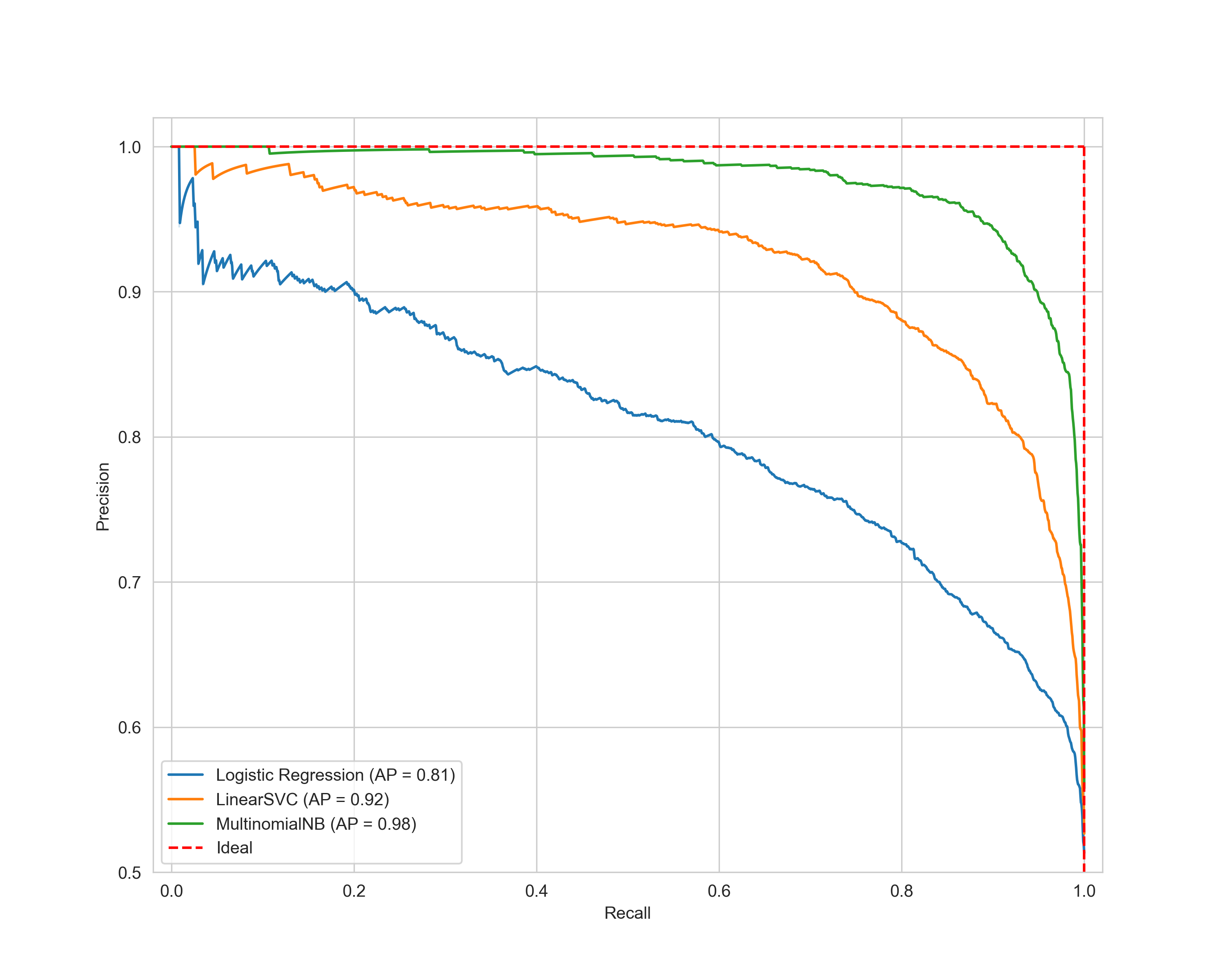
(a) Precision/Recall curve

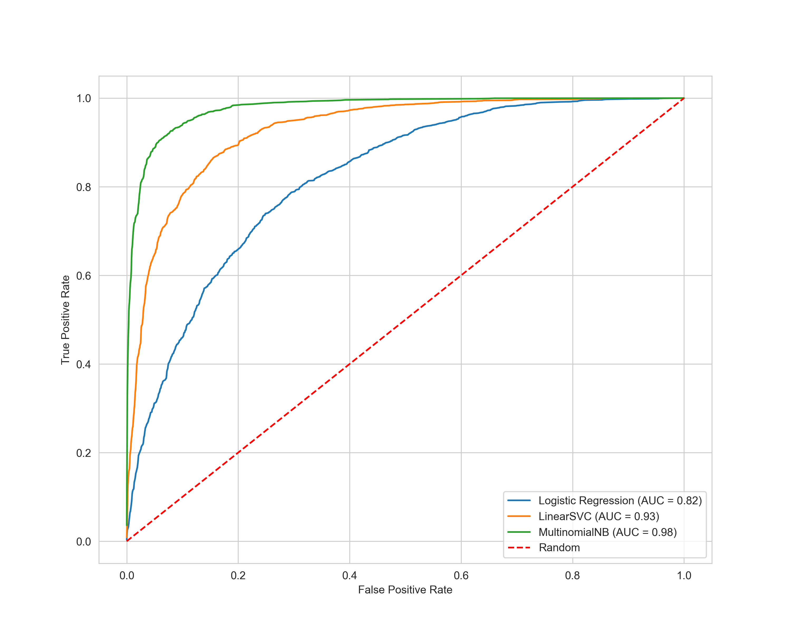
(b) ROC Curve

Figure 2: Precision/Recall and ROC Curves. (a) Shows the precision/recall curves for three models trained on the same data. The dashed line shows the ideal performance. Each model reports its Average Precision metric. (b) Shows the ROC curves for three models trained on the same data. The dashed line shows random performance. Each model reports its Area under the curve (AUC) in the legend

5 Object Detection

Object detection in deep learning is a computer vision technique that involves localizing and recognizing objects in images or videos. It is common in various applications such as autonomous driving [71, 72, 73, 74], surveillance [75, 76, 77], human-computer interaction [78, 79, 80, 81], and robotics [82, 83, 84, 85]. Object detection involves identifying the presence of an object, determining its location in an image, and recognizing the object’s class.

5.1 Object Detection Loss Functions

Since object detection involves localization (regression) and recognition (classification), object detection systems use a combination of multiple loss functions. Among these loss functions, we find:

• Multi-Class Log Loss (also known as Cross-Entropy Loss): It is used for the multi-class classification part of the object detector. Penalizes the difference between the predicted class probabilities and the ground truth class labels.

• Smooth L1 Loss: It is used for the regression part of the object detector. It aims to reduce the mean absolute error between the predicted and ground truth bounding box coordinates.

• IoU Loss: It calculates the Intersection Over Union (IoU) between the predicted bounding box and the ground truth bounding box and penalizes the difference between the predicted IoU and the ground truth IoU.

• Focal Loss: It is used to overcome the problem of class imbalance and focuses on the misclassified samples. It penalizes the samples that are easily classified with high confidence and gives more weight to the samples that are difficult to classify.

• YOLO Loss: It is used for the You Only Look Once (YOLO) object detection family of algorithms and combines the prediction of bounding box coordinates, objectness scores, and class probabilities.

In the following sections, we will delve into the loss functions that we have not touched on before or are defined differently.

5.1.1 Smooth L1 Loss

The smooth L1 loss, also known as the smooth mean absolute error (SMAE) loss, is a commonly used loss function in object detection tasks; it was introduced in Fast R-CNN [86].

The smooth L1 loss is a modification of the mean absolute error (MAE) loss that aims to balance between being too sensitive to outliers and insensitive to small errors. The formula for the smooth L1 loss is given by

$$L=\begin{cases}0.5*(x_{i}-y_{i})^{2}&\text{if }|x_{i}-y_{i}|<1\\ |x_{i}-y_{i}|-0.5&\text{otherwise},\end{cases}$$ (37)

where $x_{i}$ and $y_{i}$ are the predicted and ground truth values, respectively.

It is commonly used in the region proposal network (RPN) part of the two-stage object detectors [86, 87] to regulate the regression of the bounding box coordinates outperforming the mean square error (MSE) loss in terms of both accuracy and efficiency.

5.1.2 Intersection over Union (IoU) Loss

Intersection Over Union (IoU) is a metric used in object detection that measures the overlap between two bounding boxes. Figure 3 depicts the IoU metric used in object detection. The IoU between two bounding boxes is calculated as

$$IoU=\frac{area\ of\ intersection}{area\ of\ union}$$ (38)

The IoU loss function is defined as

$$L=1-IoU$$ (39)

This function encourages the predicted bounding boxes to overlap highly with the ground truth bounding boxes. A high IoU value indicates that the predicted bounding box is close to the ground truth, while a low IoU value indicates that the predicted bounding box is far from the ground truth.

The IoU loss function is commonly used for one-stage detectors [88, 89] as part of a multi-task loss function that includes a classification loss and a localization loss.

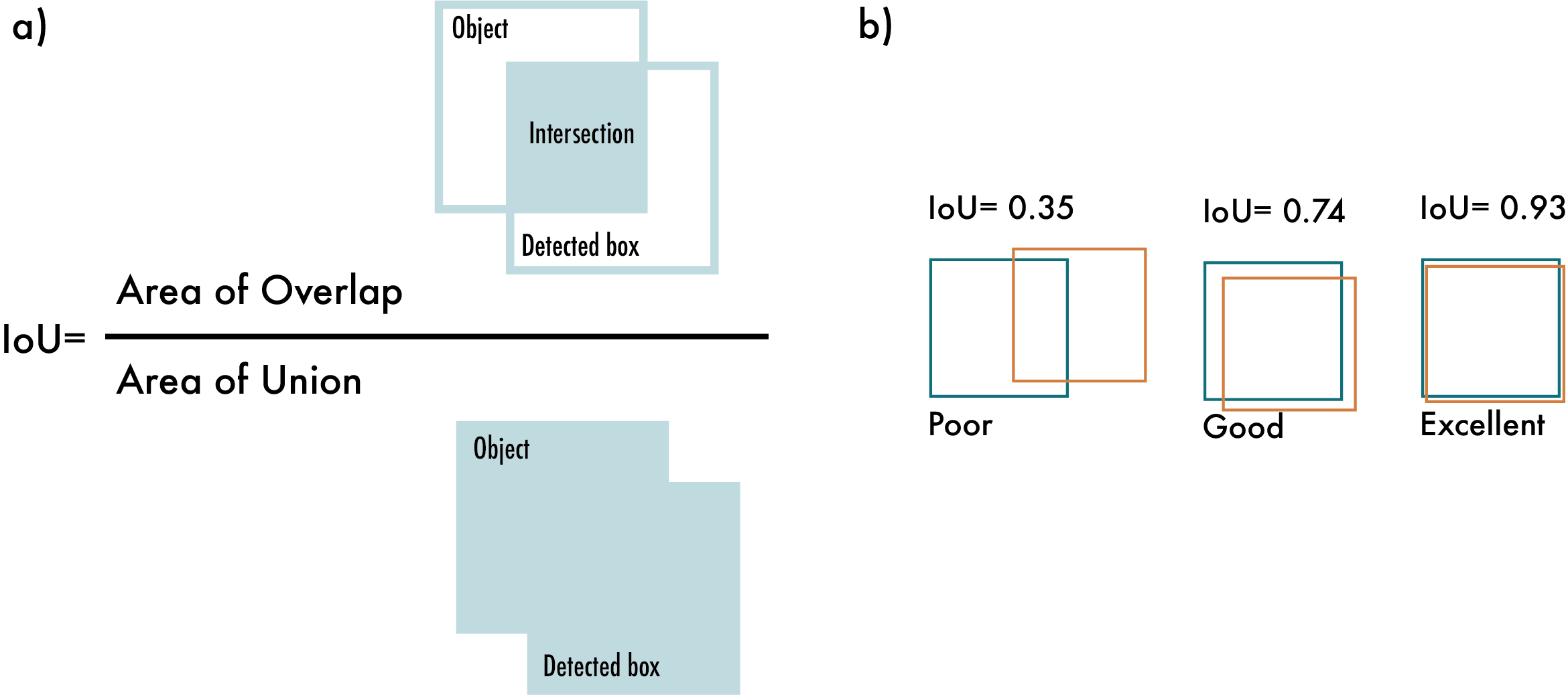
Figure 3: Intersection Over Union (IoU). a) The IoU is calculated by dividing the intersection of the two boxes by the union of the boxes; b) examples of three different IoU values for different box locations.

5.1.3 YOLO Loss

The You Only Look Once (YOLO) loss function is used in the YOLO object detection architecture. It was introduced by Redmon et al. in [90]. The YOLO loss function is a multi-part loss that consists of three components:

1. Localization loss: This component penalizes the network for misprediction of the object’s coordinates in the image. It is calculated as the mean squared error between the predicted and ground-truth bounding box coordinates.

2. Confidence loss: This component penalizes the network for not detecting an object even when one is present. It is a binary cross-entropy loss calculated between the predicted objectiveness score and the ground-truth label.

3. Classification loss: This component penalizes the network for misclassifying the object. It is a multi-class cross-entropy loss calculated between the predicted class scores and the ground-truth label.

The total YOLO loss is the weighted sum of these three components. Figure 4 explains the full YOLO loss function.

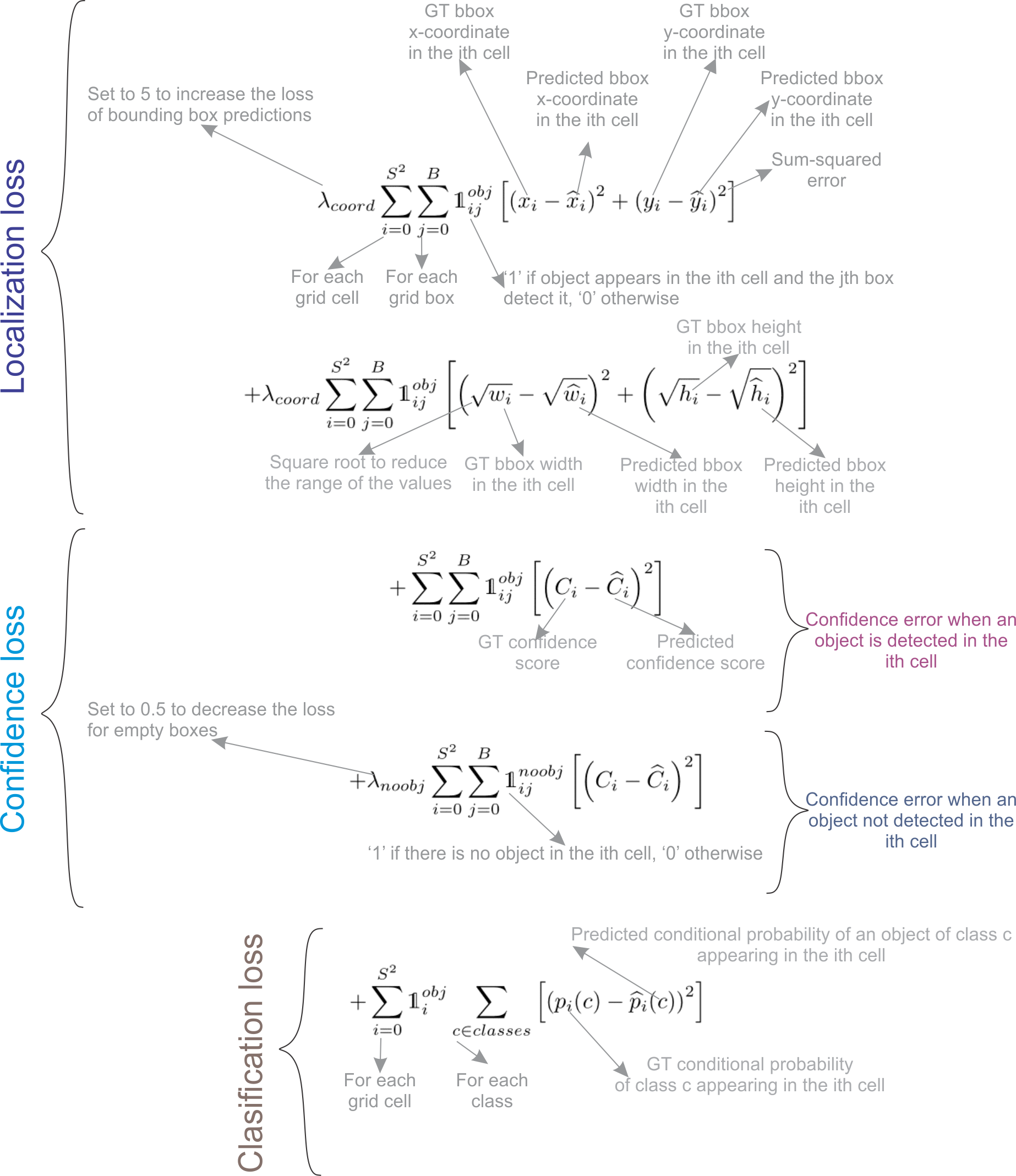
Figure 4: The YOLO Loss function comprises three parts: a localization loss, a confidence loss, and a classification loss.

5.2 Object Detection Metrics

To compute the metrics in object detection, we also compute the True Positives, False Positives, True Negatives, and False Negatives. The definitions of these metrics are based on the IoU score as follows:

True Positives in object detection: The match between the predicted location of an object and its actual location is measured using an Intersection Over Union (IoU) score. The IoU score ranges from 0 to 1, with a score of 1 indicating a perfect match between the predicted and ground-truth locations. Since a perfect match is hard to achieve, we define a threshold value to determine whether a prediction is a true positive. Common values for the threshold are 0.25, 0.5, and 0.75. These thresholds are not fixed and can be adjusted based on the application’s requirements. If the IoU score between the predicted and ground-truth boxes is greater than or equal to the defined threshold, the prediction is considered a true positive.

False Positive in object detection: Occurs when the model predicts the presence of an object, but the object is not present in the image. This affects the precision metric.

False Negative in object detection: Occurs when the model fails to detect an object that is present in an image. This affects the recall metric.

True Negative in object detection: Refers to a case where the object detector correctly determines that an object is not present in an image.

Common IoU thresholds for object detection:

• 0.5: A threshold of 0.5 is commonly used as a balanced threshold for object detection. A predicted bounding box is considered a true positive if its IoU with the ground truth bounding box is greater than or equal to 0.5.

• 0.75: A threshold of 0.75 is used for applications that require higher precision, such as autonomous driving, where false positive detections can lead to critical consequences.

• 0.25: A threshold of 0.25 is used for applications that require higher recall, such as medical image analysis, where missing detections can lead to an incorrect diagnosis.

The common object detection metrics are:

• Average Precision (AP).

• Intersection over union (IoU). See details in section 5.1.2.

• Precision-Recall Curve. See details in section 4.2.13.

5.2.1 Average Precision (AP)

Object detection models must identify and localize multiple object categories in an image. The AP metric addresses this by calculating each category’s Average Precision (AP) separately and then taking the mean of these APs across all categories (that is why it is also called mean average precision or mAP). This approach ensures that the model’s performance is evaluated for each category individually, providing a more comprehensive assessment of the model’s overall performance.

To accurately localize objects in images, AP incorporates the Intersection over Union (IoU) to assess the quality of the predicted bounding boxes. As described previously, IoU is the ratio of the intersection area to the union area of the predicted bounding box and the ground truth bounding box (see Figure 3). It measures the overlap between the ground truth and predicted bounding boxes. The COCO benchmark considers multiple IoU thresholds to evaluate the model’s performance at different levels of localization accuracy.

The two most common object detection datasets are The Pascal Visual Object Classes (VOC) [91] and Microsoft Common Objects in Context (COCO) [92]. The AP is computed differently in each of these. In the following, we describe how it is computed on each dataset.

VOC Dataset

This dataset includes 20 object categories. To compute the AP in VOC, we follow the next steps:

1. Compute Intersection over Union (IoU): For each detected object, compute the IoU with each ground truth object in the same image (refer to section 5.1.2 for more details).

2. Match Detections and Ground Truths: For each detected object, assign it to the ground truth object with the highest IoU, if the IoU is above the threshold.

3. Compute Precision and Recall: For each category, calculate the precision-recall curve by varying the confidence threshold of the model’s predictions (refer to section 4.2.13 for more details). This results in a set of precision-recall pairs.

4. Sort and interpolate with 11-points: Sort the precision-recall pairs by recall in ascending order. Then, for each recall level $r$ in the set $\{0,0.1,0.2,...,1.0\}$, find the highest precision $p(r)$ for which the recall is at least $r$. This is known as interpolated precision. This process results in a precision-recall curve that is piecewise constant and monotonically decreasing.

5. Compute Area Under Curve (AUC): The Average Precision is then defined as the area under this interpolated precision-recall curve. Since the curve is piecewise constant, this can be computed as a simple sum: $AP=sum(p(r)/N)$, where the sum is over the $N$ recall levels, and $p(r)$ is the interpolated precision at recall level $r$.

Microsoft COCO Dataset

This dataset includes 80 object categories and uses a more complex method for calculating AP. Instead of using an 11-point interpolation, it uses a 101-point interpolation, i.e., it computes the precision for 101 recall thresholds from 0 to 1 in increments of 0.01. Also, the AP is obtained by averaging over multiple IoU values instead of just one, except for a common AP metric called $AP_{50}$, which is the AP for a single IoU threshold of 0.5. Table 7 shows all the metrics used to evaluate models in the COCO dataset. The steps for computing AP in COCO are the following:

1. Compute the Intersection over Union (IoU): For each detected object, compute the IoU with each ground truth object in the same image.

2. Match Detections and Ground Truths: For each detected object, assign it to the ground truth object with the highest IoU, if this IoU is above the threshold.

3. Compute Precision and Recall: For each possible decision threshold (confidence score of the detection), compute the precision and recall of the model. This results in a set of precision-recall pairs.

4. Interpolate Precision: For each recall level $r$ in the set $\{0,0.01,0.02,...,1.00\}$ (for the 101-point interpolation used in COCO), find the maximum precision $p(r)$ for which the recall is at least $r$. This is known as interpolated precision.

5. Compute Area Under Curve (AUC): The Average Precision is then defined as the area under this interpolated precision-recall curve. Since the curve is a piecewise constant, this can be computed as a simple sum: $AP=sum(p(r))/101$, where the sum is over the 101 recall levels, and $p(r)$ is the interpolated precision at recall level $r$.

6. Average over IoU Thresholds: Repeat steps 2-5 for different IoU thresholds (e.g., 0.5, 0.55, 0.6, …, 0.95) and average the AP values.

7. Average over Categories: Repeat steps 2-6 for each category and average the AP values. This is to prevent categories with more instances from dominating the evaluation.

8. Average over Object Sizes: Finally, you can compute AP for different object sizes (small, medium, large) to see how well the model performs on different sizes of objects.

5.2.2 Average Recall (AR)

Average Recall (AR) is used to evaluate the performance of object detection models. Unlike Precision or Recall, defined at a particular decision threshold, Average Recall is computed by averaging recall values at different levels of Intersection over Union (IoU) thresholds and, if needed, at different maximum numbers of detections per image. This metric is commonly used to report COCO data results [92, 93].

The general steps to compute AR are the following:

1. Compute the Intersection over Union (IoU): For each detected object, compute the IoU with each ground truth object in the same image.

2. Match Detections and Ground Truths: For each ground truth object, find the detected object with the highest IoU. If this IoU is above a certain threshold, the detection is considered a true positive, and the ground truth is matched. Each ground truth can only be matched once.

3. Compute Recall: For each image, recall is the number of matched ground truths divided by the total number of ground truths.

4. Average over IoU Thresholds: Repeat steps 2 and 3 for different IoU thresholds (e.g., from 0.5 to 0.95 with step size 0.05), and average the recall values.

5. Average over Max Detections: Repeat steps 2-4 for different maximum numbers of detections per image (e.g., 1, 10, 100), and average the recall values. This step is necessary because allowing more detections per image can potentially increase recall but at the cost of potentially more false positives.

6. Average over Images: Finally, compute the average recall over all the images in the dataset.

For COCO, the Average Recall measure can also be computed separately for different object sizes (small, medium, and large) to evaluate how well the model works for objects of different sizes.

Table 7: COCO Evaluation Metrics.

Average Precision (AP)
AP	$\%$ AP at IoU=.50:.05:.95 (primary challenge metric)
$AP^{IoU=.50}$	$\%$ AP at IoU=.50 (PASCAL VOC metric)
$AP^{IoU=.75}$	$\%$ AP at IoU=.75 (strict metric)
AP Across Scales:
$AP^{small}$	$\%$ AP for small objects: area $<32^{2}$
$AP^{medium}$	$\%$ AP for medium objects: $32^{2}<$ area $<96^{2}$
$AP^{large}$	$\%$ AP for large objects: area $>96^{2}$
Average Recall (AR):
$AR^{max=1}$	$\%$ AR given 1 detection per image
$AR^{max=10}$	$\%$ AR given 10 detections per image
$AR^{IoU=100}$	$\%$ AR given 100 detection per image
AR Across Scales:
$AR^{small}$	$\%$ AR for small objects: area $<32^{2}$
$AR^{medium}$	$\%$ AR for medium objects: $32^{2}<$ area $<96^{2}$
$AR^{large}$	$\%$ AR for large objects: area $>96^{2}$

6 Image Segmentation

Image segmentation aims to assign a label or category to each pixel in the image, effectively segmenting the objects at a pixel level. Segmentation is usually performed using deep learning models trained to classify each pixel in the image based on its features and context. Segmentation methods are mainly classified into three categories: semantic segmentation [94, 95, 96, 97, 98, 99, 100, 101], instance segmentation [102, 103, 104, 105, 106], and panoptic segmentation [107, 108, 109, 110, 111].

Semantic Segmentation studies the uncountable stuff in an image. It analyzes each image pixel and assigns a unique class label based on the texture it represents. In a street image, the semantic segmentation’s output will assign the same label to all the cars and the same image to all the pedestrians; it cannot differentiate the objects separately.

Instance Segmentation deals with countable things. It can detect each object or instance of a class present in an image and assigns it to a different mask or bounding box with a unique identifier.

Panoptic Segmentation presents a unified segmentation approach where each pixel in a scene is assigned a semantic label (due to semantic segmentation) and a unique instance identifier (due to instance segmentation).

Segmentation applications include scene understanding [112, 113, 114, 115, 116], medical image analysis [117, 118, 119, 120, 121, 122, 123], robotic perception [124, 125, 126, 127, 128], autonomous vehicles [129, 130, 131, 132, 133, 134], video surveillance [135, 136, 137, 138, 139], and augmented reality [140, 141, 142, 143, 144].

6.1 Segmentation Loss Functions

Common loss functions include cross-entropy loss, Intersection over union (IoU) loss, Focal loss, Dice loss, Tversky loss, and Lovász Loss. The following sections will describe these loss functions and their applications.

6.1.1 Cross Entropy Loss for Segmentation

The cross-entropy loss for segmentation measures the dissimilarity between the predicted and ground truth segmentation maps. The cross-entropy loss is calculated by comparing the predicted and ground truth segmentation maps pixel-by-pixel [95]. It is defined as the negative log-likelihood of the ground truth segmentation map given the predicted segmentation map. The cross-entropy loss is calculated using the following formula:

$$-\frac{1}{N}\sum\limits_{i=1}^{N}\sum\limits_{c=1}^{C}y_{i,c}log(p_{i,c}),$$ (40)

where $N$ is the total number of pixels in the image, $C$ is the number of classes, $y$ is the ground truth segmentation map, and $p$ is the predicted segmentation map. The values of $y$ and $p$ should be between 0 and 1 and sum up to 1. The lower the cross-entropy loss, the better the prediction.

6.1.2 Intersection Over Union (IoU) loss for segmentation

The Intersection Over Union (IoU) loss is a commonly used loss function and evaluation metric for semantic segmentation tasks. The goal is to predict a per-pixel segmentation mask for a given image. The IoU loss is also known as the Jaccard loss or Jaccard Index (JI), and is defined as the ratio of the intersection of the predicted and ground-truth masks to the union of the predicted and ground-truth masks. The IoU loss is calculated per-pixel basis, and the final loss is the average IoU across all pixels in the image.

The IoU loss can be defined mathematically as:

$$IoU=\frac{1}{n}\sum_{i=1}^{n}\frac{y_{i}\cap\hat{y}_{i}}{y_{i}\cup\hat{y}_{i}},$$ (41)

where $y_{i}$ is the ground-truth mask for pixel $i$, $\hat{y}_{i}$ is the predicted mask, $y_{i}\cap\hat{y}_{i}$ is the intersection of the ground-truth and predicted masks, and $y_{i}\cup\hat{y}_{i}$ is the union of the ground-truth and predicted masks.

IoU is commonly used in various semantic segmentation works as a loss function [145, 146] and as an evaluation metric[94, 147].

6.1.3 Dice Loss

The Dice loss, also known as the Dice similarity coefficient [148], is used to evaluate the similarity between the predicted segmentation mask and the ground truth mask. The loss function is defined as

$$L=1-\frac{2\cdot intersection(pred,gt)}{|pred|+|gt|},$$ (42)

where $pred$ is the predicted segmentation mask, $gt$ is the ground truth segmentation mask, $intersection(pred,gt)$ is the number of pixels that are in the intersection of the predicted and ground truth masks, and $|pred|$ and $|gt|$ are the total number of pixels in the predicted and ground truth masks, respectively.

Dice loss is widely used in medical imaging, where the goal is to segment structures in images with high precision.

6.1.4 Tversky loss

The Tversky loss [149] is a variation of the Dice loss, commonly used in image segmentation tasks. It is defined as

$$Tversky(A,B)=\frac{|A\cap B|}{|A\cap B|+\alpha|A\backslash B|+\beta|B\backslash A|},$$ (43)

where $A$ and $B$ are the predicted and ground truth segmentation masks, respectively, and $\alpha$ and $\beta$ are user-defined hyperparameters that control the weighting of false positives and false negatives.

This loss function is similar to the Dice loss, but it allows the assignment of different weights to false positives and false negatives, which can be useful in certain scenarios where the imbalance between the two types of errors is significant.

6.1.5 Lovász Loss

The main idea behind the Lovász Loss[150] is to optimize the IoU by optimizing the Jaccard index or IoU between the predicted segmentation and the ground-truth segmentation. This loss function is particularly useful in image segmentation tasks where the Intersection-over-Union (IoU) score is highly important. The Lovász Loss is defined as the sum of the predicted segmentation mask and the ground-truth segmentation mask, weighted by the Jaccard index as follows:

$$L=-\frac{1}{N}\sum_{i=1}^{N}Jaccard(p_{i},y_{i})\log(p_{i}),$$ (44)

where $N$ is the number of pixels in the image, $p$ is the predicted segmentation mask, and $y$ is the ground-truth segmentation mask.

The Lovász loss provides a differentiable surrogate for the non-differentiable IoU metric, allowing it to be optimized directly.

6.2 Segmentation Metrics

The common metrics for evaluating segmentation are the Mean Intersection over union (mIoU), pixel accuracy, Average Precision (AP) (refer to section 5.2.1), BF score, and Panoptic Quality. The following sections will explain each, skipping IoU, and AP already discussed.

6.2.1 Pixel Accuracy

Measures the proportion of correctly classified pixels in the whole image. It is calculated by dividing the number of correctly classified pixels by the total number of pixels in the image. The formula for pixel accuracy is

$$Pixelaccuracy=\frac{\text{Number of correctly classified pixels}}{\text{Total number of pixels in image}}$$ (45)

Like regular accuracy, pixel accuracy can be misleading when the class imbalance is high, as it does not consider false positives or negatives. This is why other metrics, such as Intersection over Union (IoU) or Dice coefficient, are commonly used to evaluate image segmentation models.

6.2.2 Boundary F1 Score (BF)

The Boundary F1 Score (BF) [151], often abbreviated as BF score, is a metric used for evaluating image segmentation quality, particularly when the precision of the boundary location is important. The BF score applies the concept of the F1 score to the segmentation boundaries rather than the segment regions themselves.

The computation of the BF score involves the following steps:

1. For each segment in the ground truth, find the closest predicted segment (according to some distance measure, often the mean shortest distance between the boundaries of the two segments).

2. Compute the precision as the proportion of predicted segments close enough to a ground truth segment. Formally, this is $P=TP/(TP+FP)$, where $TP$ (True Positive) is the number of predicted segments close enough to a ground truth segment, and $FP$ (False Positive) is the number of predicted segments not close enough to any ground truth segment.

3. Compute the recall as the proportion of ground truth segments close enough to a predicted segment. Formally, this is $R=TP/(TP+FN)$, where $FN$ (False Negative) is the number of ground truth segments not close enough to any predicted segment.

4. The BF score is then the harmonic mean of precision and recall:

$$F\_score=\frac{2*Precision*Recall}{Precision+Recall}$$ (46)

A threshold is typically defined as close enough when matching predicted segments to ground truth segments. The BF score ranges from 0 to 1, with 1 indicating a perfect match between the predicted and ground truth boundaries.

6.2.3 Panoptic Quality (PQ)

Panoptic Quality (PQ) is a metric proposed for evaluating panoptic segmentation tasks [107].

The Panoptic Quality metric is defined as:

$$PQ=\frac{\Sigma_{(p,g)\in TP}IoU(p,g)}{|TP|}\times\frac{|TP|}{|TP|+\frac{1}{2}|FP|+\frac{1}{2}|FN|},$$ (47)

where

• IoU(p, g) denotes the intersection-over-union of prediction p and ground truth g.

• TP (True Positive) is a set of matched pairs of predicted and ground truth segments.

• FP (False Positive) is a set of predicted segments not matched with any ground truth segment.

• FN (False Negative) is a set of ground truth segments not matched with any predicted segment.

The PQ metric ranges between 0 and 1, where 1 signifies a perfect segmentation. It is a product of two terms:

The first term, called segmentation quality (SQ), calculates the average IoU of the correctly predicted segments (true positives). This term measures how accurately each detected object has been segmented and thus rewards prediction quality.

The second term, called Recognition Quality (RQ), calculates the ratio of the number of true positives to the total number of segments. This term measures how accurately each object has been recognized.

This metric can be more informative than mean IoU when dealing with complex scenes containing multiple object instances per class, as it considers both the segmentation quality and the correct recognition of distinct instances.

7 Face Recognition

Face recognition aims to accurately match an individual’s face in an image or video to a corresponding entry in a database of faces. This task is often performed using deep learning algorithms, such as Convolutional Neural Networks (CNNs) or Transformers [152], that are trained on large datasets of face images. The algorithms are trained to extract features from images faces and then use these features to recognize faces that match those in the database. Face recognition has many applications, including security [153, 154], social media [155], and biometric identification systems [156, 157].

7.1 Face Recognition Loss Functions and Metrics

The loss functions used in face recognition are typically aimed at preserving the structure and similarity of the input faces. They can be divided into two classes: loss functions based on classification and loss functions based on representation learning. Common loss functions based on classification are softmax loss, A-softmax loss, Center loss, Large-Margin cosine loss, and Additive Angular Margin loss. On the other hand, loss functions based on representation learning are Triplet loss, Contrastive loss, Circle loss, and the Barlow twins loss.

The metrics commonly used for face recognition are the same as the ones used for classification, such as accuracy, precision, recall, F1-score, ROC, etc.

In the following subsections, we will describe each of these loss functions.

7.1.1 Softmax Loss

The Softmax Loss computes the cross-entropy between the predicted class probabilities and the true class label, followed by the logarithmic operation to convert the negative log-likelihood into a loss value. The final loss is obtained by summing the cross-entropy over all classes and all samples.

Let’s denote the weight vectors for each class (or, in this case, each face identity) as $W=\{w_{1},w_{2},...,w_{n}\}$, where $n$ is the number of classes (or identities). For a given input image $x$ of class $y$, the linear classifier would compute a score $f(x,W)=Wx+b$, where $b$ is the bias term.

The softmax function converts these scores into probabilities. The probability of the $i^{th}$ class is computed as follows:

$$P(y=i|x;W)=\frac{e^{w_{i}^{T}x+b_{i}}}{\sum_{j=1}^{n}e^{w_{j}^{T}x+b_{j}}}$$ (48)

The softmax loss (also known as the cross-entropy loss) for an input-output pair $(x,y)$ is defined as the negative log-likelihood of the correct class, which we can be expressed as

$$L_{i}=-\log(P(y=y_{i}|x;W))=-f_{y_{i}}+\log\sum_{j=1}^{n}e^{f_{j}},$$ (49)

where $f_{y_{i}}$ is the score for the correct class, and $f_{j}$ are the scores for all classes. The total loss for a batch of data is the mean of $L_{i}$ over all the examples in the batch.

The disadvantage of this loss function is that it does not have fine-grained control over the intra-class and inter-class distances that come in handy for face recognition purposes.

7.1.2 A-Softmax Loss

The A-Softmax loss [158], also known as the SphereFace loss, was designed to address the limitations of the traditional softmax loss by considering the angular information between the features of face images and their corresponding labels. The A-Softmax loss aims to maximize the inter-class separability and minimize the intra-class variations of face features.

Given a weight matrix $W$, an input feature vector $x$, and a margin parameter $m$, the SphereFace loss is calculated as follows:

1. Compute the Normalized weight matrix $W_{norm}$ as

$$W_{norm}=\frac{W}{||W||}$$ (50)

where each column $w_{i}$ in $W_{norm}$ is a unit vector, i.e., $||w_{i}||=1$. The normalization operation makes the weights for each class lie on the unit hypersphere.

2. Compute the margin $M$ to be applied to the angles:

$$M=(m-1)\cdot y_{true}+1$$ (51)

In this equation, $y_{true}$ is the true class label. If $y_{true}$ equals 1, $M$ equals $m$, and if $y_{true}$ equals 0, $M$ equals 1.

3. Compute the cosine of the angle $\theta$ between the feature vector $x$ and the weight vector:

$$cos(\theta)=\frac{W_{norm}\cdot x}{||x||},$$ (52)

where $||\cdot||$ denotes the L2 norm.

4. Compute the new angle $\theta^{\prime}$ and its cosine after applying the margin:

$$\theta^{\prime}=\theta\cdot M$$ (53)

$$cos(\theta^{\prime})=cos(\theta^{\prime})$$

5. Compute the new prediction $y_{pred}^{\prime}$ by rescaling with the norm of $x$:

$$y_{pred}^{\prime}=||x||\cdot cos(\theta^{\prime})$$ (54)

6. Finally, compute the SphereFace loss $L$, which is the negative log-likelihood of the true class:

$$L=-\log\frac{\sum y_{true}\cdot e^{y_{pred}^{\prime}}}{\sum e^{y_{pred}^{\prime}}}$$ (55)

Here, the summation is taken over all classes. The numerator is the exponentiated prediction for the true class, and the denominator is the sum of exponentiated predictions for all classes.

Compared to the traditional softmax loss, the A-Softmax loss produces more discriminative and compact features, improving face recognition performance.

7.1.3 Center Loss

The center loss [159] aims to increase the inter-class variance while reducing the intra-class variance by penalizing the distances between the features of a sample and the center of its corresponding class. The center loss is inspired by the idea of having a center for each class in the feature space, and the loss function encourages the features of the same class to be close to its center. The center loss is defined as the Euclidean distance between the feature of a sample and the center of its class in the feature space.

The center loss is usually added to the main loss function in the training process, and it is defined as

$$L_{center}=\frac{1}{2}\sum_{i=1}^{n}\left|\mathbf{x_{i}}-\mathbf{c_{y_{i}}}\right|_{2}^{2},$$ (56)

where $\mathbf{x_{i}}$ is the feature representation of the $i^{th}$ sample, $y_{i}$ is its corresponding class label, $\mathbf{c_{y_{i}}}$ is the center of class $y_{i}$, and $n$ is the number of samples.

7.1.4 CosFace: Large-Margin Cosine Loss

CosFace loss, also known as the Large Margin Cosine Loss, maximizes the decision margin in the cosine space to further enhance the discriminative power of the deeply learned features.

The cosine of the angle between the feature vector $x_{i}$ and the weight $w_{j}$ of the $j^{th}$ class is given by

$$cos\theta_{j}=\frac{w_{j}^{T}x_{i}}{||w_{j}||||x_{i}||},$$ (57)

where $||.||$ denotes the l2 norm.

The CosFace method adds a cosine margin $m$ to the target logit, so the modified cosine of the angle $\theta_{y_{i}}$ corresponding to the ground truth class $y_{i}$ is given by:

$$cos\theta_{y_{i}}-m$$ (58)

Then the CosFace loss for an input-output pair $(x_{i},y_{i})$ is defined as

$$L_{i}=-\log\frac{e^{s(cos\theta_{y_{i}})-m}}{e^{s(cos\theta_{y_{i}})-m}+\sum_{j\neq y_{i}}^{n}e^{scos\theta_{j}}},$$ (59)

where $s$ is a scaling factor.

One advantage of this function is that the cosine function’s non-monotonicity does not create a problem here, unlike SphereFace. Also, because the feature vector is normalized, the model must learn better separation of the angles as it cannot reduce loss by learning a different norm [160].

7.1.5 ArcFace. Additive Angular Margin Loss

The ArcFace loss [161] enhances the discriminative power of the softmax loss by adding an angular margin penalty to the target logit.

The ArcFace method adds an additive angular margin $m$ to the target logit, so the modified cosine of the angle $\theta_{y_{i}}$ corresponding to the ground truth class $y_{i}$ is given by

$$cos(\theta_{y_{i}}+m)$$ (60)

Then the ArcFace loss for an input-output pair $(x_{i},y_{i})$ is defined as

$$L_{i}=-\log\frac{e^{scos(\theta_{y_{i}}+m)}}{e^{scos(\theta_{y_{i}}+m)}+\sum_{j\neq y_{i}}^{n}e^{scos\theta_{j}}},$$ (61)

where $s$ is a scaling factor. The margin $m$ can be interpreted as an additional arc length on the hypersphere of radius $s$. Experiments show better inter-class discrepancy than Triplet Loss while having about the same intra-class similarity [160].

7.1.6 Triplet Loss

Probably the best-known loss function for face recognition. The idea behind the triplet loss [162, 163] is to train the model to distinguish between a positive pair of images (two images of the same person) and a negative pair of images (two images of different persons).

Given an anchor image, $A$, a positive image, $P$, and a negative image, $N$, (see Figure 5), the loss is calculated as the distance between the anchor image and positive image and the distance between the anchor image and negative image, plus a margin. The equation is defined as

$$L_{triplet}=\max{0,\left\lVert\textbf{f}_{A}-\textbf{f}_{P}\right\rVert^{2}_{2}-\left\lVert\textbf{f}_{A}-\textbf{f}_{N}\right\rVert^{2}_{2}+\alpha},$$ (62)

where $\textbf{f}_{A}$, $\textbf{f}_{P}$, and $\textbf{f}_{N}$ are the embeddings of the anchor image, positive image, and negative image, respectively, and $\alpha$ is a hyperparameter known as the margin. By minimizing this loss, the embeddings of the positive images get closer to each other than the embeddings of the negative images.

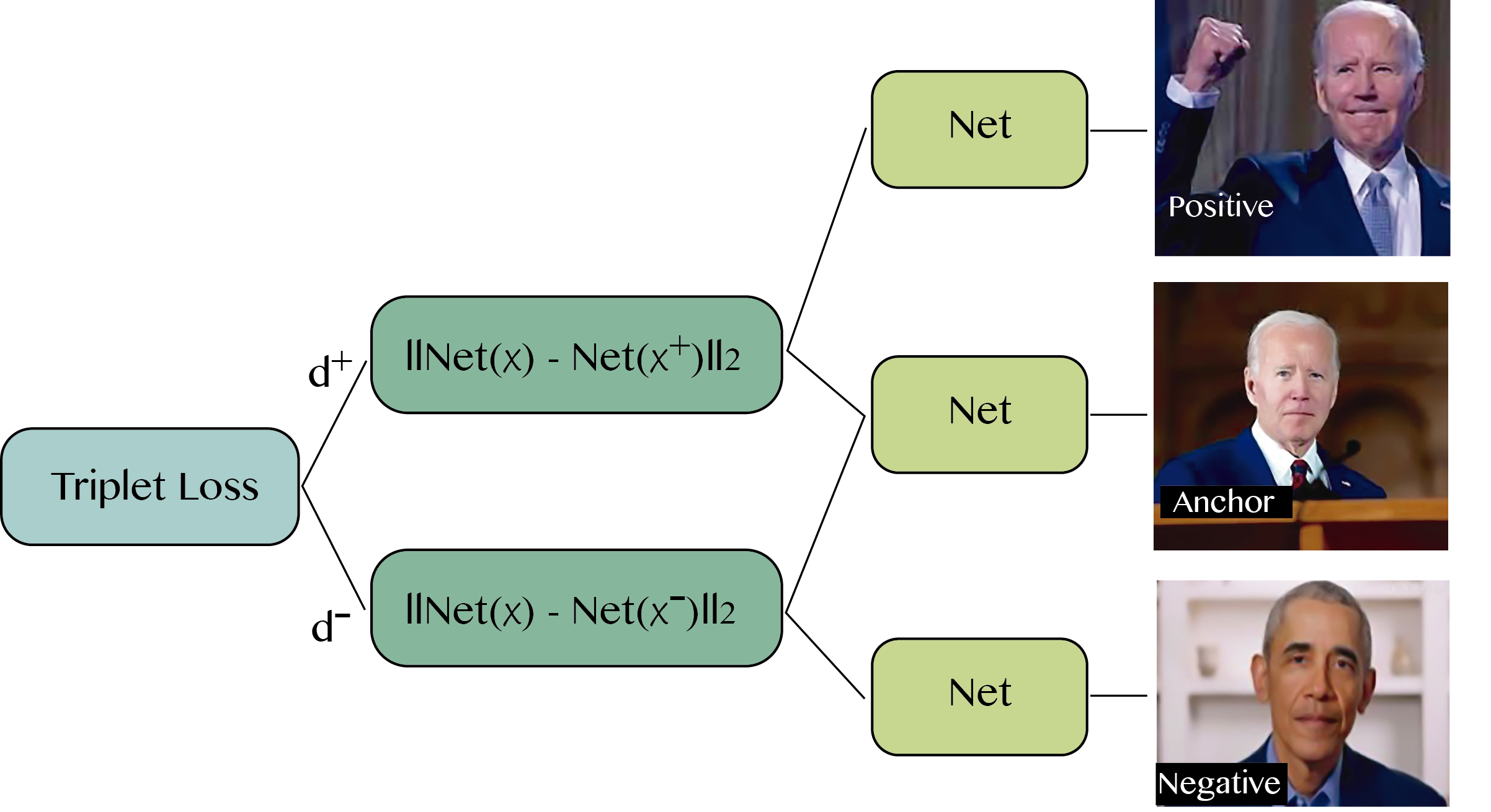
Figure 5: Triplet Loss. Given an anchor image, a positive image, and a negative image, the triplet loss computes the distance between the embeddings of the anchor image and positive image and the distance between the embeddings of the anchor image and negative image. By minimizing this loss, the embeddings of the positive images get closer to each other than the embeddings of the negative images.

7.1.7 Contrastive Loss

The contrastive loss [164] learns a feature representation or image embedding that projects similar images close to each other and dissimilar images far apart. This loss is based on a Siamese architecture of the neural network. The contrastive loss function is defined as:

$$L=\frac{1}{N}\sum_{i=1}^{N}y_{i}\left|f(x_{i}^{a})-f(x_{i}^{p})\right|_{2}^{2}+(1-y_{i})\max\left(0,m-\left|f(x_{i}^{a})-f(x_{i}^{n})\right|_{2}^{2}\right),$$ (63)

where $f(x_{i}^{a})$ is the deep feature representation of the anchor image $x_{i}^{a}$, $f(x_{i}^{p})$ is the deep feature representation of the positive image $x_{i}^{p}$, $f(x_{i}^{n})$ is the deep feature representation of the negative image $x_{i}^{n}$. $y_{i}$ is a binary label indicating whether the anchor and positive images are similar (1) or dissimilar (0), $m$ is a margin hyperparameter, and $N$ is the number of triplets in the batch.

The margin $m$ controls how hard the model should work to push dissimilar embeddings apart. Extending a trained model for new/unseen classes is easy because it learns to create a semantic representation of the image rather than classify it among a predetermined set of classes.

One limitation of this loss is that the margin $m$ is the same constant for all dissimilar pairs, which implicitly pushes the model to have the same distance between all dissimilar pairs, even if some are more dissimilar [160, 165]. A second limitation is that the absolute notion of similar and dissimilar pairs is not transferable from one context to another [166].

7.1.8 Circle Loss

The Circle Loss [167] pushes positive pairs closer and negative pairs farther away while maintaining a circle-like decision boundary. This is achieved by adding margins to positive and negative pairs, enlarging the intra-class variance for negative pairs, and reducing the intra-class variance for positive pairs. By doing so, Circle Loss can effectively handle imbalanced data and complex distributions, which are common challenges in face recognition tasks. The circle loss equation can be expressed as

$$\alpha_{pos_{i}} =\max(O_{pos_{i}}-s_{pos_{i}},0)$$ (64)

$$\alpha_{neg_{j}} =\max(O_{neg_{j}}-s_{neg_{j}},0)$$

$$sum_{pos} =\sum_{i}e^{-\gamma\cdot\alpha_{pos_{i}}\cdot_{pos_{i}}}$$

$$sum_{neg} =\sum_{j}e^{\gamma\cdot\alpha_{neg_{j}}\cdot s_{neg_{j}}}$$

$$L =\log(1+sum_{pos}\cdot sum_{neg})$$

Where:

• $s_{pos_{i}}$ and $s_{neg_{j}}$ represent the pairwise similarity between the positive and negative pairs. The positive pairs belong to the same class, and the negative pairs belong to different classes.

• $O_{pos_{i}}$ and $O_{neg_{j}}$ represent the user-defined margins for positive and negative pairs, respectively. $O_{pos}$ is a margin that should be smaller than the expected similarity of positive pairs, while $O_{neg}$ should be larger than the expected similarity of negative pairs. Thus, you want to choose $O_{pos}$ and $O_{neg}$ such that $O_{pos}<O_{neg}$.

• $\alpha_{pos_{i}}$ and $\alpha_{neg_{j}}$ are slack variables that ensure the positive similarities are larger than $O_{pos_{i}}$ and the negative similarities are smaller than $O_{neg_{j}}$. This is achieved by setting the minimum value to 0, ignoring similarities that have already met the margin requirement.

• $sum_{pos}$ and $sum_{neg}$ are exponentiated and scaled sums of the positive and negative similarities, respectively. The exponential function ensures that all values are positive and emphasize larger values, while $\gamma$ is a scaling factor that controls the rate at which the emphasis increases. The slack variables $\alpha_{pos_{i}}$ and $\alpha_{neg_{j}}$ are used in the exponent to give more weight to pairs far from meeting the margin requirement.

• Finally, $L$ is the Circle Loss computed as the logarithm of 1 plus the product of $sum_{pos}$ and $sum_{neg}$. This encourages both $sum_{pos}$ and $sum_{neg}$ to be small, which in turn encourages the positive similarities to be large and the negative similarities to be small. Adding one inside the logarithm ensures that the argument is always positive, and the logarithm itself helps dampen the effect of large values and reduce the effect of outliers.

The circle loss has a more definite convergence target than the triplet loss because there is a single point in the ($s_{neg}$, $s_{pos}$) space toward which the optimization is driven ($O_{neg}$, $O_{pos}$). However, choosing ($O_{neg}$, $O_{pos}$) is arbitrary. In practice, it is common to use cross-validation or a separate validation set to tune these hyperparameters.

A common strategy is to start with small margins and gradually increase them. If the margins are too large, the model struggles to learn; if they are too small, it learns embeddings that are not discriminative enough. In some implementations of Circle Loss, $O_{pos}$ and $O_{neg}$ are not independent but related by a constant margin $m$, which is set to ensure a sufficient gap between positive and negative pairs. In this case, we only need to tune one of the margins or the gap $m$.

7.1.9 Barlow Twins Loss

The Barlow Twins loss [168] is a self-supervised learning approach. The key idea is to make the outputs of a two-twin network, processing two different views of the same image, as similar as possible while reducing the redundancy between the dimensions of these representations. It encourages the network to learn highly informative features about the input and non-redundant.

Given the batch size $N$ and the dimensionality $D$ of the embeddings, the network processes two different augmentations of the same input data, producing the embeddings $z_{a}$ and $z_{b}$. These embeddings are then normalized to have zero mean and unit variance along the batch dimension.

The computation of the Barlow Twins loss can be formulated as follows: 1. Compute the cross-correlation matrix $C$:

$$C=\frac{1}{N}z_{a_{norm}}^{T}\cdot z_{b_{norm}}$$ (65)

2. Compute the difference matrix $C_{diff}$ between the cross-correlation matrix and an identity matrix and square it:

$$C_{diff}=(C-I)^{2}$$ (66)

3. Scale the off-diagonal elements of $C_{diff}$ by a factor $\lambda$:

$$C_{diff_{ij}}=\begin{cases}C_{diff_{ij}},&\text{if }i=j\\ \lambda C_{diff_{ij}},&\text{if }i\neq j\end{cases}$$ (67)

4. Finally, the Barlow Twins loss $L$ is the sum of all elements in the updated $C_{diff}$:

$$L=\sum_{i,j}C_{diff_{ij}}$$ (68)

By backpropagating this loss and updating the model’s parameters, the network is trained to minimize redundancy and increase the similarity between two different views of the same image, learning more robust and informative features as a result.

This method does not require a fixed number of classes and does not suffer from data expansion as it does not require explicit negative examples. However, the model in the paper required large dimensionality of the final representation for good performance, and the performance is not robust to remove certain distortions to the inputs [160].

7.1.10 SimSiam Loss

SimSiam [169] is a self-supervised learning aimed at learning representations by pushing two views of the same image to be as similar as possible. While it is not explicitly designed for face recognition, it can be used to learn meaningful representations of faces.

Given two different augmentations $x_{1}$ and $x_{2}$ of the same image, they are forwarded through a neural network and a prediction head to obtain the features $z_{1},z_{2}$ and the predictions $p_{1},p_{2}$.

The loss is defined as the negative cosine similarity between the predictions and the features of the different augmentations.

$$L=-\frac{1}{2}[\frac{(p_{1}^{T}z_{2})}{(||p_{1}||\cdot||z_{2}||)}+\frac{(p_{2}^{T}z_{1})}{(||p_{2}||\cdot||z_{1}||)}],$$ (69)

where ^T denotes transpose, and $||\cdot||$ denotes the L2 norm.

This loss encourages the model to make the predictions $p_{1}$ and $p_{2}$ as similar as possible to the features $z_{2}$ and $z_{1}$, respectively.

An important part of the SimSiam approach is a stop-gradient operation applied to $z_{2}$ in the first term and $z_{1}$ in the second term of the loss function. This means that the gradients are not backpropagated through these variables during training. The stop-gradient operation is critical to avoid the model collapsing into trivial solutions where the features and the predictions are the same.

The advantages of the SimSiam loss are:

1. No Negative Pair: Unlike contrastive learning methods that require negative examples, SimSiam does not require any. This simplifies the model training process and can make it more efficient.

2. Stop-Gradient Operation: The use of stop-gradient operation in SimSiam makes it less prone to collapsing into trivial solutions. This is a significant advantage because many self-supervised learning models struggle with this problem.

3. Simplicity: SimSiam is simpler compared to other self-supervised learning methods. It uses a symmetric architecture and a simple loss function which encourages two views of the same image to have similar representations.

The disadvantages include:

1. Hyperparameter Sensitivity: SimSiam has a few crucial hyperparameters, such as the learning rate and weight decay, which require careful tuning to get the best performance. Incorrect settings can significantly degrade the model’s performance.

2. Dependence on Data Augmentation: The success of SimSiam, like many other self-supervised learning models, heavily relies on the choice and quality of data augmentations. This requires domain knowledge and potentially significant effort to determine the most effective augmentations.

3. Non-semantic Features: One common issue with self-supervised learning methods, including SimSiam is that the features learned may not necessarily be semantically meaningful. They are good at capturing low-level features but may not be as effective in capturing high-level semantic information.

8 Image Generation

Image generation in deep learning involves using artificial neural networks to generate new images. This task has been revolutionized by developing various models such as Variational Autoencoders (VAEs) [170, 171, 172, 173], Generative Adversarial Networks (GANs) [174, 175, 176, 177, 178], Normalized Flow models (NFs) [179, 180, 181, 182, 183], Energy-Based Models (EBMs) [184, 185, 186, 187, 188, 189], and Diffusion Models [190, 191, 192, 193, 194]. These models allow the generation of high-quality images that can be used in various applications such as image super-resolution [195, 196, 197, 198], denoising [199, 200, 201], inpainting [202, 203, 204, 205], and style transfer [206, 207, 208, 209].

Variational Autoencoders (VAEs) are generative models that use deep learning techniques to create new data and learn latent representations of the input data. VAEs consist of two primary components: an encoder and a decoder. The encoder takes input data and compresses it into a lower-dimensional latent space, capturing the essential features of the data. This is typically a probabilistic process, producing a mean and standard deviation representing potential latent space values distribution. The decoder then takes a point from this latent space distribution and reconstructs the original data. The entire process is trained in such a way as to minimize the difference between the original and the reconstructed data, as well as to ensure the latent space approximates a standard Gaussian distribution. VAEs can generate new data by feeding the decoder points sampled from the latent space.

Generate Adversarial Networks (GANs) involve two neural networks, a Generator, and a Discriminator, playing a game against each other. The Generator tries to create data similar to the training data, while the Discriminator tries to distinguish between the real and generated data. Through this process, both networks improve: the Generator learns to produce increasingly realistic data, while the Discriminator becomes better at distinguishing between real and artificial data. This adversarial process continues until an equilibrium is reached, at which point the Generator is producing realistic data and the Discriminator is, at best, randomly guessing whether the data is real or generated. This equilibrium is conceptually referred to as a Nash equilibrium in game theory [210].

Normalizing Flow Models (NFs) can construct complex probability distributions by transforming a simple base distribution through a sequence of invertible and differentiable transformations, or flows. These flows warp and twist the data space, allowing the model to generate diverse outputs. The parameters of these transformations are learned from data using maximum likelihood estimation. An advantage of Normalizing Flows over other generative models is their ability to provide an exact and tractable likelihood for a given sample, enabling efficient sampling and density estimation. However, they can be computationally intensive to train due to the need to compute and backpropagate through the Jacobian of the flows.

Energy-Based Models (EBMs) learn a scalar energy function to distinguish real data points from unlikely ones, assigning lower energy values to points similar to the training data and higher values otherwise. A neural network often parameterizes this function and learns from the data. Sampling in EBMs is typically done via Markov Chain Monte Carlo (MCMC) [211] methods, producing samples distributed according to the learned energy function. While EBMs can represent a wide variety of data distributions, they can be challenging to train due to the intractability of the partition function and the computational expense of MCMC sampling.

Diffusion models can create new data by simulating a random process, specifically a diffusion process. The process starts with a simple data distribution (e.g., Gaussian noise) and gradually transforms it towards the target data distribution, like a particle undergoing diffusion or a random walk. This transformation is controlled by a neural network trained to model the reverse process, taking real-world data and applying a series of transformations to reduce it to noise. During generation, an initial noise sample is iteratively updated using this reverse process model, running the process backward, leading to a sample from the target data distribution. This approach allows the generation of complex and high-quality data, such as images, by simulating a smooth transition from noise to the desired data.

The following sections will review the common lost functions and performance metrics used for image generation.

8.1 Image Generation Loss functions

The loss function in a VAE consists of the reconstruction loss and the Kullback-Leibler (KL) (refer to section 8.1.2). The reconstruction loss measures how well the decoded data matches the original input data. The KL divergence measures how much the learned distribution in the latent space deviates from a target distribution, usually a standard normal distribution. KL-divergence is used as a regularization term to ensure that the distributions produced by the encoder remain close to a unit Gaussian, penalizing the model if the learned distributions depart from it.

The most common loss function used in GANs is the adversarial loss, which is the sum of the cross-entropy loss between the generator’s predictions and the real or fake labels. More recently, WGAN [212] applied the Wasserstein distance as an alternative to training GANs to improve the stability and avoid mode collapse that occurs when the generator network stops learning the underlying data distribution and begins to produce a limited variety of outputs, rather than a diverse range of outputs that accurately represent the true data distribution.

Normalizing Flows are typically trained using maximum likelihood estimation. Given a dataset, the aim is to maximize the log-likelihood of the data under the model by minimizing the negative log-likelihood of the data.

During training, Energy-based models (EBMs) minimize a loss function that encourages the energy function to assign lower energy values to data points from the training data and higher energy values to other points. Different types of EBMs use different loss functions, such as Contrastive Divergence (CD)[213], Maximum Likelihood Estimation (MLE)[214], and Noise-Contrastive Estimation (NCE) [215].

Diffusion models use a denoising loss function based on the Mean Absolute Error (MAE) or the Mean Squared Error (MSE) between the original and reconstructed data.

In the next sections, we describe in detail each of these losses.

8.1.1 Reconstruction Loss

The purpose of the reconstruction loss is to ensure that the decoder network of the VAE can reconstruct an input image that is as close as possible to the original image. In essence, the reconstruction loss compares the original image to the reconstructed image and penalizes any difference between the two. The reconstruction loss is calculated as the mean squared error (MSE) between the original image and the reconstructed image, which is defined as follows

$$L_{recon}=\frac{1}{N}\sum_{i=1}^{N}||x_{i}-\hat{x_{i}}||^{2},$$ (70)

where $x_{i}$ is the original image, $\hat{x_{i}}$ is the reconstructed image, and $N$ is the number of images.

Another metric that can be used for reconstruction loss is binary cross-entropy (BCE), a common choice for binary images. The BCE loss can be defined as:

$$L_{BCE}=-\sum_{i=1}^{n}y_{i}\log(\hat{y_{i}})+(1-y_{i})\log(1-\hat{y_{i}}),$$ (71)

where $y_{i}$ is the binary value of the original image and $\hat{y_{i}}$ is the binary value of the generated image.

In the context of deep learning, reconstruction loss has been used in various image generation tasks such as image restoration, image generation, and image synthesis.

8.1.2 Kullback-Leibler Divergence Loss

The KL divergence loss, also known as the KL divergence loss, measures the difference between the predicted probability distribution and the true probability distribution of the classes [216]. The KL divergence loss ensures that the predicted probabilities are close to the true probabilities, which can be useful in cases where the true probabilities are known or can be approximated.

The KL divergence loss is defined as

$$KL(p||q)=\sum_{i=1}^{n}p(x_{i})log(\frac{p(x_{i})}{q(x_{i})}),$$ (72)

where $p(x_{i})$ is the true probability of class $x_{i}$ and $q(x_{i})$ is the predicted probability of class $x_{i}$.

The KL divergence loss is often used in generative models such as variational autoencoders, which aim to approximate the true data distribution. It is also used in reinforcement learning to ensure that the agent’s learned policy is close to the optimal policy.

One disadvantage of using the KL divergence loss is that it is sensitive to zero probabilities in the true probability distribution. This can lead to numerical instability and can make the loss function difficult to optimize. To overcome this issue, a common practice is to add a small value (e.g., $1e-7$) to the true probability distribution to avoid zero probabilities.

8.1.3 Adversarial Loss

The adversarial loss is the main function used in Generative Adversarial Networks (GANs). It is based on the idea of a minimax game between the two neural networks. The adversarial loss is used to train the generator, defined as the negative log-likelihood of the discriminator’s output.

Goodfellow et al. first introduced the adversarial loss in [174]. The authors showed that this loss function leads to the convergence of the generator to a Nash equilibrium, where the generator produces realistic images that the discriminator cannot distinguish from real images.

The adversarial loss can be defined as:

$$L_{adv}(G,D)=-\mathbb{E}{x\sim p{data}(x)}[\log D(x)]-\mathbb{E}_{z\sim p_{z}(z)}[\log(1-D(G(z)))],$$ (73)

where $G$ is the generator network, $D$ is the discriminator network, $x$ are real images from the data distribution $p_{data}(x)$, $z$ are random noise inputs from the noise distribution $p_{z}(z)$, and $G(z)$ are generated images.

The adversarial loss encourages the generator to generate indistinguishable images from real images and the discriminator to correctly classify real images and generated images. The training process alternates between updating the generator and the discriminator until the generator produces realistic images.

8.1.4 Wasserstein loss

The Wasserstein loss [212] is used in generative models, such as Generative Adversarial Networks (GANs), to measure the difference between the real and generated distributions. The Wasserstein loss is the minimum work required to transform one probability distribution into another. The amount of work is the sum of the distances between each sample multiplied by their probability mass. The Wasserstein loss can be written as

$$W(p_{data},p_{gen})=\inf_{\gamma\in\Gamma(p_{data},p_{gen})}\int_{x,y}||x-y||d\gamma(x,y)$$ (74)

where $p_{data}$ and $p_{gen}$ represent the real and generated distributions, respectively. $\Gamma(p_{data},p_{gen})$ is the set of joint distributions with marginals $p_{data}$ and $p_{gen}$, and $\gamma(x,y)$ is the joint distribution of $(x,y)$.

The Wasserstein loss has been widely used in GANs for its ability to provide a more stable training process and to avoid the mode collapse problem, where the generator produces a limited number of similar outputs.

8.1.5 Negative Log-likelihood in Normalizing Flows

In Normalizing Flows, the objective is to learn a transformation (or a sequence of transformations) that maps a complex data distribution to a simpler distribution, for example, a standard Gaussian. The transformations are chosen such that their Jacobian determinant is easy to compute, which allows using the change of variables formula to compute the likelihood of the data under the model.

Given a data point $x$, let’s denote $z=f_{\theta}(x)$ as the mapping of $x$ to the base distribution under the flows parameterized by $\theta$, and $p_{z}(z)$ as the density of the base distribution. Then, the log-likelihood of $x$ under the model is given by

$$\log p_{\theta}(x)=\log p_{z}(f_{\theta}(x))-\log\left|\det\frac{\partial f_{\theta}(x)}{\partial x}\right|$$ (75)

The second term is the log absolute determinant of the Jacobian of the transformation, which corrects for the change in volume due to the transformation.

The loss function that we minimize during training is the negative log-likelihood of the data. If our dataset consists of $N$ points $x_{1},x_{2},\ldots,x_{N}$, then the loss function $L(\theta)$ is expressed as

$$L(\theta)=-\frac{1}{N}\sum_{i=1}^{N}\log p_{\theta}(x_{i})=-\frac{1}{N}\sum_{i=1}^{N}\left[\log p_{z}(f_{\theta}(x_{i}))-\log\left|\det\frac{\partial f_{\theta}(x_{i})}{\partial x_{i}}\right|\right]$$ (76)

In practice, stochastic gradient descent or a variant minimizes this loss function and learns the parameters $\theta$ of the flows.

Normalizing Flows are computationally intensive to train, due to the need to compute and backpropagate through the Jacobian of the flows. For this reason, methods such as RealNVP [179] and Glow [180] are designed so that the determinant of the Jacobian can be computed efficiently.

8.1.6 Contrastive Divergence

Contrastive Divergence (CD) can be used in training Energy-Based Models (EBMs), specifically for estimating the log-likelihood gradient. As with RBMs, the objective is to maximize the likelihood of the data under the model. The key difference is that the energy function is defined over the visible and hidden units in EBMs, whereas it’s defined over the joint configuration of visible and hidden units in RBMs.

In many energy-based models, the log-likelihood gradient involves an expectation over all possible data configurations, which is generally intractable to compute exactly. CD approximates this expectation by running a Markov chain for several steps.

Given a dataset consisting of N data points $x_{1},x_{2},...,x_{N}$, the log-likelihood of the data under the model is:

$$L(\theta)=\frac{1}{N}\sum_{i=1}^{N}\log p(x_{i};\theta),$$ (77)

where $\theta$ represents the parameters of the model, and $p(x;\theta)$ is the probability of data point $x$, defined as $p(x;\theta)=\frac{e^{-E(x;\theta)}}{Z(\theta)}$, with $E(x;\theta)$ being the energy function and $Z(\theta)$ the partition function.

The gradient of the log-likelihood for the parameters is

$$\frac{\partial}{\partial\theta}L(\theta)=\frac{1}{N}\sum_{i=1}^{N}\frac{\partial}{\partial\theta}\log p(x_{i};\theta)$$ (78)

This gradient can be decomposed into two terms: the positive phase, which is easy to compute

$$\frac{1}{N}\sum_{i=1}^{N}\frac{\partial E(x_{i};\theta)}{\partial\theta}$$ (79)

and the negative phase, which involves an expectation over all model configurations and is generally intractable.

$$-\langle\frac{\partial E(x;\theta)}{\partial\theta}\rangle_{p},$$ (80)

where $\langle\rangle_{p}$ denotes an expectation with respect to the model distribution.

In CD, the negative phase is approximated by running a Markov chain starting from a data point for a few steps and using the resulting sample to estimate the expectation. This leads to the CD-k algorithm, where k is the number of Gibbs sampling steps. The update to the parameters after seeing a data point $x$ is then

$$\Delta\theta=\eta(\frac{1}{N}\sum_{i=1}^{N}\frac{\partial E(x_{i};\theta)}{\partial\theta}+\langle\frac{\partial E(x^{\prime};\theta)}{\partial\theta}\rangle_{CD}),$$ (81)

where $\eta$ is the learning rate, $\langle\rangle_{CD}$ denotes an expectation to the distribution defined by the Markov chain after k steps, and $x^{\prime}$ is the sample obtained after k steps of Gibbs sampling starting from a data point $x$.

Contrastive Divergence is often more computationally efficient than other methods for training energy-based models, such as Persistent Contrastive Divergence (PCD) [217] or Mean-Field methods [218] because it requires running the Markov chain for a few steps rather than until it reaches equilibrium. However, this introduces a bias in the estimate of the gradient of the log-likelihood. CD is a suitable choice when the bias is acceptable or can be mitigated by running the chain for more steps.

8.2 Image Generation Metrics

Some of the common metrics used for Image generation are:

• Peak Signal-to-Noise Ratio (PSNR)

• Structural Similarity Index (SSIM)

• Inception Score (IS) [219]

• Frechet Inception Distance (FID) [220]

In the following sections, we will dive into each of these metrics.

8.2.1 Peak Signal-to-Noise Ratio (PSNR)

Peak Signal-to-Noise Ratio (PSNR) is a traditional metric often used to assess the quality of image and video codecs, comparing the original and the reconstructed (compressed and then decompressed) images or videos. It is a measure of the quality of an approximation of an image.

In image generation, PSNR can be used to evaluate the quality of the images generated by models, particularly for tasks like image super-resolution, denoising, inpainting, etc. Here, the PSNR is used to compare the images generated by the model to a ground truth high-quality image.

The PSNR is defined in terms of the mean squared error (MSE), which for two $m\times n$ monochrome images $I$ and $K$ where one of the images is considered a noisy approximation of the other is defined as

$$MSE=\frac{1}{mn}\sum_{i=0}^{m-1}\sum_{j=0}^{n-1}[I(i,j)-K(i,j)]^{2}$$ (82)

The PSNR is defined as

$$PSNR=10\cdot\log_{10}\left(\frac{(MAX_{I})^{2}}{MSE}\right),$$ (83)

where $MAX_{I}$ is the maximum possible pixel value of the image. For instance, for an 8-bit grayscale image, this value would be 255.

PSNR provides an easily interpretable score as expressed in a logarithmic decibel scale. Higher PSNR generally indicates that the reconstruction is of high quality; however, in some cases, perceptually similar images may have low PSNR where simple pixel-wise errors do not well capture structural similarity.

While PSNR could be useful in the context of tasks like super-resolution or denoising where there is a clear ground truth to compare to, it is not particularly effective for tasks like generative image modeling where the goal is to produce new, high-quality images that are not simply reconstructions of existing images [221]. More sophisticated metrics like the Inception Score or Fréchet Inception Distance are typically used for these tasks.

8.2.2 Structural Similarity Index (SSIM)

The Structural Similarity Index (SSIM) [222] can be used in image generation tasks to compare the generated images with the target (real) images. In other words, it measures how similar the synthetic images produced by a generative model are to the actual images. The SSIM index is based on three main factors: luminance, contrast, and structure. The SSIM value ranges from -1 to 1, where 1 indicates perfect similarity, and -1 indicates no similarity.

To calculate the SSIM index, the first step is to compute each image’s mean and standard deviation, then the cross-covariance between the two images, and the product of the standard deviations. The SSIM index is then computed as

$$SSIM(x,y)=\frac{(2\mu_{x}\mu_{y}+C_{1})(2\sigma_{xy}+C_{2})}{(\mu_{x}^{2}+\mu_{y}^{2}+C_{1})(\sigma_{x}^{2}+\sigma_{y}^{2}+C_{2})},$$ (84)

where $\mu_{x}$ and $\mu_{y}$ are the means of images $x$ and $y$, $\sigma_{x}$ and $\sigma_{y}$ are the standard deviations of images $x$ and $y$, $\sigma_{xy}$ is the cross-covariance between the two images, and $C_{1}$ and $C_{2}$ are constants used to avoid instability.

The SSIM metric is more robust to brightness and contrast changes than other popular image quality metrics, such as the Mean Squared Error (MSE) and the Peak Signal-to-Noise Ratio (PSNR). However, using SSIM alone as an evaluation metric for generative models is insufficient because the ultimate goal of a generative model is not just to reproduce an exact copy of the input image but to understand the underlying data distribution. For this reason, SSIM is often used in conjunction with other metrics, such as Inception Score (IS) and Fréchet Inception Distance (FID), to evaluate the performance of generative models more comprehensively.

8.2.3 Inception Score (IS)

The Inception Score (IS) quantifies the quality and diversity of generated images [219]. It is computed by combining two scores: the marginal likelihood of the generated images and their quality or diversity. The marginal likelihood is calculated by feeding the generated images into an Inception-v3 classifier trained on the ImageNet dataset and taking the average of the softmax probabilities. Their overall scores determine the quality of the images, while the entropy of these scores reflects the diversity.

The formula for the inception score can be expressed as

$$IS=e^{(\mathbb{E}_{x\sim p_{g}(x)}[KL(p(y|x)||p(y))])},$$ (85)

where $p_{g}(x)$ is the distribution of generated images, $p(y|x)$ is the class conditional probability for each image and class, and $p(y)$ is the marginal likelihood of each class.

The Inception Score provides a single number that reflects the quality of generated images and the diversity of these objects and it is easy to calculate using pre-trained Inception models that don’t require the true data distribution as input.

However, the Inception Score has some limitations that make it insufficient to comprehensively understand the model performance:

1. Inception Model Dependence: Relies heavily on the Inception model, which is pre-trained on the ImageNet dataset. This may limit its usefulness in domains that are very different from ImageNet, as the features learned by the Inception model might not be relevant for those domains.

2. Mismatch with Human Perception: It does not always align with human perception of image quality. Images can achieve high IS by simply being diverse and recognizable, even if they don’t look real.

3. Lack of Discrimination Between Modes: It can be high for models that cover many modes of the true data distribution but fail to accurately capture the frequency of those modes.

4. Doesn’t Measure Mode Collapse: As mentioned before, a problem in training GANs is mode collapse, where the model generates a limited range of images. The Inception Score can’t effectively detect mode collapse as long as the few modes that the GAN does generate are diverse enough.

5. Unreliable for Low Number of Samples: When computed over a small number of samples, the Inception Score can become unreliable due to high variance.

8.2.4 Fréchet Inception Distance (FID)

Unlike the Inception Score, the Fréchet Inception Distance (FID) [220] considers the statistics of the images generated by the model and compares them to the statistics of real images. It measures the distance between these two distributions in a feature space provided by a specific layer of the Inception network.

Mathematically, the FID is defined as follows. Let us denote the generated images as $X$ and the real images as $Y$. Each dataset is passed through an Inception network, and the activations at a specific layer are extracted. The resulting activations are denoted as $X^{\prime}$ and $Y^{\prime}$ respectively. Assuming that $X^{\prime}$ and $Y^{\prime}$ are multivariate Gaussian distributions with means $\mu_{x}$ and $\mu_{y}$, and covariance matrices $\Sigma_{x}$ and $\Sigma_{y}$, respectively, the Fréchet distance between these two multivariate Gaussian distributions is defined as

$$FID(X^{\prime},Y^{\prime})=||\mu_{x}-\mu_{y}||^{2}+Tr(\Sigma_{x}+\Sigma_{y}-2(\Sigma_{x}\Sigma_{y})^{1/2}),$$ (86)

where $Tr$ is the trace of a matrix, which is the sum of its diagonal elements, $(\Sigma_{x}\Sigma_{y})^{1/2}$ is the matrix square root of the product of the covariance matrices, which is well-defined since the covariance matrices are positive semi-definite.

FID has the following desirable properties:

1. Lower value is better: The lower the FID score, the closer the generated image distribution is to the real image distribution.

2. Considers both mean and covariance: FID considers both the means and the covariance of the feature representations, giving it an advantage over metrics considering only one of these aspects.

3. Less susceptible to noise: FID is more robust to noise compared to the Inception Score.

Regarding the limitations, like the Inception Score, it relies on the Inception network and, therefore, may not perform well on tasks very different from the ImageNet dataset on which the Inception network was trained.

9 Discussion

Throughout this paper, we have reviewed a variety of loss functions and metrics utilized in deep learning, specifically focusing on different tasks, including regression, classification, object detection, image segmentation, and face recognition. Our review underscores the importance of selecting an appropriate loss function and evaluation metric, depending on the specific task at hand and the characteristics of the data.

For regression tasks, for instance, Mean Squared Error (MSE) and Mean Absolute Error (MAE) are widely used due to their simplicity and interpretability. However, there are more robust alternatives such as Huber loss or application specific such as Quantile or Poisson loss. Additionally, while RMSE and MAE are commonly used for evaluation, they may need to adequately capture the performance of models on all types of data, leading to the use of additional metrics such as $R^{2}$ and Adjusted $R^{2}$.

In classification, it is noted that while binary cross-entropy loss is standard for binary classification tasks, options such as hinge loss and weighted binary cross-entropy can provide robustness in situations where classes are imbalanced. Furthermore, more than accuracy is required to provide a complete picture of a model’s performance, especially in imbalanced datasets. This necessitates using additional metrics like precision, recall, F1-score, and AUC-ROC.

The complexity increases when we consider object detection, image segmentation, and face recognition tasks. Here, loss functions are about more than just calculating the difference between the predicted and true values. For instance, the YOLO loss in object detection and image segmentation, or the Triplet Loss in face recognition, considers the relative positions and distances of multiple instances or entities.

Moreover, metrics used in these tasks, such as Average Precision (AP) and Average Recall (AR) for object detection or Panoptic Quality (PQ) for Panoptic segmentation, go beyond typical accuracy-based metrics to evaluate the quality of instance identification and segmentation.

As discussed, each loss function and metric has pros and cons, and their appropriateness may depend on the specific application or dataset characteristics. Understanding these trade-offs is critical for the design of effective deep learning systems.

Looking forward, there are opportunities for developing new loss functions and metrics that are more robust to data anomalies, consider specific practical constraints, or are tailored to new and emerging deep learning tasks. We also see potential in automated methods that intelligently select or combine different loss functions and metrics based on the given task and data.

By advancing our understanding of these critical components of deep learning, we can continue to push the boundaries of what these powerful models can achieve.

10 Conclusion

The choice of the loss function and metric can profoundly influence the performance of a model; hence understanding their nature and implications is helpful for anyone working in deep learning.

From regression to complex tasks such as object detection, face recognition, and generative models, we have highlighted the importance of utilizing appropriate loss functions and evaluation metrics. Furthermore, considering dataset characteristics, specifically class imbalances and outliers, was vital when designing and evaluating models. There is no one-size-fits-all loss function or metric for every task. This highlights the continued necessity for researchers to develop task-specific or adaptable loss functions and metrics and further refine the performance and applicability of deep learning models.

A promising direction for future work is the exploration of automated methods to intelligently select or combine loss functions and metrics, thereby reducing the manual effort and potential bias involved in their selection. In addition, creating robust loss functions that can handle data anomalies and practical constraints effectively is a fertile area for exploration.

The ability to accurately model and predict complex phenomena is increasingly critical in our rapidly evolving digital world. By enhancing our comprehension and application of loss functions and metrics in deep learning, we can significantly contribute to advancing this technology, paving the way for future more sophisticated, effective, and reliable models.

11 Acknowledgments

We thank the National Council for Science and Technology (CONACYT) for its support through the National Research System (SNI) and the project SIP 20232290.

Declaration of generative AI and AI-assisted technologies in the writing process

During the preparation of this work, the authors used GPT-4 for help with wording, formatting, and styling throughout this work. After using this tool, the authors reviewed and edited the content as needed and take full responsibility for the publication’s content.

References

- [1] J. Smith, “Deep learning for image recognition,” Journal of Artificial Intelligence, vol. 15, no. 2, pp. 78–95, 2018.
- [2] E. Jones, “Object detection using neural networks,” Computer Vision Review, vol. 8, no. 4, pp. 112–128, 2020.
- [3] M. Gonzalez, “Image segmentation using neural networks,” Pattern Recognition, vol. 22, no. 1, pp. 36–52, 2017.
- [4] L. Wang, “Facial recognition using neural networks,” IEEE Transactions on Pattern Analysis and Machine Intelligence, vol. 37, no. 6, pp. 1100–1112, 2019.
- [5] W. Chen, “Image generation using adversarial neural networks,” ACM Transactions on Graphics.
- [6] L. Chen, “Automatic speech recognition with neural networks,” IEEE Transactions on Audio, Speech, and Language Processing, vol. 27, no. 6, pp. 1200–1212, 2019.
- [7] W. Liu, “Speech emotion recognition with neural networks,” IEEE Transactions on Affective Computing, vol. 11, no. 3, pp. 500–512, 2020.
- [8] M. Kim, “Multilingual speech recognition with neural networks,” Speech Communication, vol. 101, pp. 50–63, 2018.
- [9] P. Zhang, “Robust speech recognition with neural networks,” Computer Speech and Language, vol. 65, pp. 101–120, 2021.
- [10] H. Wu, “End-to-end speech recognition with neural networks,” IEEE Signal Processing Letters, vol. 24, no. 11, pp. 1631–1635, 2017.
- [11] J. Smith, “Sentiment analysis using natural language processing,” Journal of Artificial Intelligence, vol. 15, no. 2, pp. 78–95, 2018.
- [12] E. Jones, “Named entity recognition using natural language processing,” Computational Linguistics, vol. 46, no. 4, pp. 112–128, 2020.
- [13] M. Gonzalez, “Text summarization using natural language processing,” ACM Transactions on Information Systems, vol. 35, no. 2, pp. 36–52, 2017.
- [14] L. Wang, “Part-of-speech tagging using natural language processing,” Journal of Machine Learning Research, vol. 20, no. 7, pp. 1100–1112, 2019.
- [15] W. Chen, “Question answering using natural language processing,” IEEE Transactions on Knowledge and Data Engineering, 2021.
- [16] L. A. Gatys, A. S. Ecker, and M. Bethge, “Image style transfer using convolutional neural networks,” IEEE Conference on Computer Vision and Pattern Recognition (CVPR), pp. 2414–2423, 2016.
- [17] K. Zhang, W. Zuo, Y. Chen, D. Meng, and L. Zhang, “Beyond a gaussian denoiser: Residual learning of deep cnn for image denoising,” IEEE Transactions on Image Processing, vol. 26, no. 7, pp. 3142–3155, 2017.
- [18] T. Karras, T. Aila, S. Laine, and J. Lehtinen, “Progressive growing of gans for improved quality, stability, and variation,” International Conference on Learning Representations (ICLR), 2018.
- [19] D. Harrison Jr and D. L. Rubinfeld, “Hedonic housing prices and the demand for clean air,” Journal of environmental economics and management, vol. 5, no. 1, pp. 81–102, 1978.
- [20] H.-x. Zhao and F. Magoulès, “A review on the prediction of building energy consumption,” Renewable and Sustainable Energy Reviews, vol. 16, no. 6, pp. 3586–3592, 2012.
- [21] F. E. Harrell Jr, K. L. Lee, R. M. Califf, D. B. Pryor, and R. A. Rosati, “Regression modelling strategies for improved prognostic prediction,” Statistics in medicine, vol. 3, no. 2, pp. 143–152, 1984.
- [22] S. Shen, H. Jiang, and T. Zhang, “Stock market forecasting using machine learning algorithms,” Department of Electrical Engineering, Stanford University, Stanford, CA, pp. 1–5, 2012.
- [23] E. C. Malthouse and R. C. Blattberg, “Can we predict customer lifetime value?,” Journal of interactive marketing, vol. 19, no. 1, pp. 2–16, 2005.
- [24] E. L. Lehmann and G. Casella, Theory of point estimation. Springer Science & Business Media, 2006.
- [25] C. J. Willmott and K. Matsuura, “Advantages of the mean absolute error (mae) over the root mean square error (rmse) in assessing average model performance,” Climate research, vol. 30, no. 1, pp. 79–82, 2005.
- [26] A. Auslender and M. Teboulle, “Interior gradient and epsilon-subgradient descent methods for constrained convex minimization,” Mathematics of Operations Research, vol. 29, no. 1, pp. 1–26, 2004.
- [27] Y. Bai, Q. Jiang, and J. Sun, “Subgradient descent learns orthogonal dictionaries,” arXiv preprint arXiv:1810.10702, 2018.
- [28] P. Bianchi, W. Hachem, and S. Schechtman, “Stochastic subgradient descent escapes active strict saddles on weakly convex functions,” arXiv preprint arXiv:2108.02072, 2021.
- [29] L. Xiao, “Dual averaging method for regularized stochastic learning and online optimization,” Advances in Neural Information Processing Systems, vol. 22, 2009.
- [30] P. J. Huber, “Robust estimation of a location parameter,” Breakthroughs in statistics: Methodology and distribution, pp. 492–518, 1992.
- [31] R. A. Saleh, A. Saleh, et al., “Statistical properties of the log-cosh loss function used in machine learning,” arXiv preprint arXiv:2208.04564, 2022.
- [32] R. Koenker and K. F. Hallock, “Quantile regression,” Journal of economic perspectives, vol. 15, no. 4, pp. 143–156, 2001.
- [33] M.-Y. Chen and J.-E. Chen, “Application of quantile regression to estimation of value at risk,” Review of Financial Risk Management, vol. 1, no. 2, p. 15, 2002.
- [34] J. Bruzda, “Multistep quantile forecasts for supply chain and logistics operations: bootstrapping, the garch model and quantile regression based approaches,” Central European Journal of Operations Research, vol. 28, no. 1, pp. 309–336, 2020.
- [35] J. B. Bremnes, “Probabilistic wind power forecasts using local quantile regression,” Wind Energy: An International Journal for Progress and Applications in Wind Power Conversion Technology, vol. 7, no. 1, pp. 47–54, 2004.
- [36] W. P. Gaglianone and L. R. Lima, “Constructing density forecasts from quantile regressions,” Journal of Money, Credit and Banking, vol. 44, no. 8, pp. 1589–1607, 2012.
- [37] L. Massidda and M. Marrocu, “Quantile regression post-processing of weather forecast for short-term solar power probabilistic forecasting,” Energies, vol. 11, no. 7, p. 1763, 2018.
- [38] A. Zarnani, S. Karimi, and P. Musilek, “Quantile regression and clustering models of prediction intervals for weather forecasts: A comparative study,” Forecasting, vol. 1, no. 1, pp. 169–188, 2019.
- [39] J. Zietz, E. N. Zietz, and G. S. Sirmans, “Determinants of house prices: a quantile regression approach,” The Journal of Real Estate Finance and Economics, vol. 37, pp. 317–333, 2008.
- [40] R. Winkelmann, “Reforming health care: Evidence from quantile regressions for counts,” Journal of Health Economics, vol. 25, no. 1, pp. 131–145, 2006.
- [41] A. C. Cameron and P. K. Trivedi, Regression analysis of count data, vol. 53. Cambridge university press, 2013.
- [42] H. Yang, K. Ozbay, and B. Bartin, “Effects of open road tolling on safety performance of freeway mainline toll plazas,” Transportation research record, vol. 2324, no. 1, pp. 101–109, 2012.
- [43] J. Viel, “Poisson regression in epidemiology,” Revue D’epidemiologie et de Sante Publique, vol. 42, no. 1, pp. 79–87, 1994.
- [44] Y. Mouatassim and E. H. Ezzahid, “Poisson regression and zero-inflated poisson regression: application to private health insurance data,” European actuarial journal, vol. 2, no. 2, pp. 187–204, 2012.
- [45] H. Shen and J. Z. Huang, “Forecasting time series of inhomogeneous poisson processes with application to call center workforce management,” The Annals of Applied Statistics, vol. 2, no. 2, pp. 601–623, 2008.
- [46] P. Avila Clemenshia and M. Vijaya, “Click through rate prediction for display advertisement,” International Journal of Computer Applications, vol. 975, p. 8887, 2016.
- [47] D. Lambert, “Zero-inflated poisson regression, with an application to defects in manufacturing,” Technometrics, vol. 34, no. 1, pp. 1–14, 1992.
- [48] D. W. Osgood, “Poisson-based regression analysis of aggregate crime rates,” Journal of quantitative criminology, vol. 16, pp. 21–43, 2000.
- [49] P. Goodwin and R. Lawton, “On the asymmetry of the symmetric mape,” International journal of forecasting, vol. 15, no. 4, pp. 405–408, 1999.
- [50] X. Tian, H. Wang, and E. Erjiang, “Forecasting intermittent demand for inventory management by retailers: A new approach,” Journal of Retailing and Consumer Services, vol. 62, p. 102662, 2021.
- [51] D. Ramos, P. Faria, Z. Vale, and R. Correia, “Short time electricity consumption forecast in an industry facility,” IEEE Transactions on Industry Applications, vol. 58, no. 1, pp. 123–130, 2021.
- [52] S. Kumar Chandar, “Grey wolf optimization-elman neural network model for stock price prediction,” Soft Computing, vol. 25, pp. 649–658, 2021.
- [53] M. Lawrence, M. O’Connor, and B. Edmundson, “A field study of sales forecasting accuracy and processes,” European Journal of Operational Research, vol. 122, no. 1, pp. 151–160, 2000.
- [54] K.-F. Chu, A. Y. Lam, and V. O. Li, “Deep multi-scale convolutional lstm network for travel demand and origin-destination predictions,” IEEE Transactions on Intelligent Transportation Systems, vol. 21, no. 8, pp. 3219–3232, 2019.
- [55] N. J. Nagelkerke et al., “A note on a general definition of the coefficient of determination,” Biometrika, vol. 78, no. 3, pp. 691–692, 1991.
- [56] J. Miles, “R-squared, adjusted r-squared,” Encyclopedia of statistics in behavioral science, 2005.
- [57] R. Goodman, J. Miller, and P. Smyth, “Objective functions for neural network classifier design,” in Proceedings. 1991 IEEE International Symposium on Information Theory, pp. 87–87, 1991.
- [58] S. Jadon, “A survey of loss functions for semantic segmentation,” in 2020 IEEE conference on computational intelligence in bioinformatics and computational biology (CIBCB), pp. 1–7, IEEE, 2020.
- [59] E. A. Nadaraya, “On estimating regression,” Theory of Probability & Its Applications, vol. 9, no. 1, pp. 141–142, 1964.
- [60] C. Szegedy, V. Vanhoucke, S. Ioffe, J. Shlens, and Z. Wojna, “Rethinking the inception architecture for computer vision,” in Proceedings of the IEEE conference on computer vision and pattern recognition, pp. 2818–2826, 2016.
- [61] R. Müller, S. Kornblith, and G. E. Hinton, “When does label smoothing help?,” Advances in neural information processing systems, vol. 32, 2019.
- [62] T.-Y. Lin, P. Goyal, R. Girshick, K. He, and P. Dollár, “Focal loss for dense object detection,” in Proceedings of the IEEE international conference on computer vision, pp. 2980–2988, 2017.
- [63] M. S. Hossain, J. M. Betts, and A. P. Paplinski, “Dual focal loss to address class imbalance in semantic segmentation,” Neurocomputing, vol. 462, pp. 69–87, 2021.
- [64] T. He, Y. Liu, C. Shen, X. Wang, and C. Sun, “Instance-aware embedding for point cloud instance segmentation,” in Computer Vision–ECCV 2020: 16th European Conference, Glasgow, UK, August 23–28, 2020, Proceedings, Part XXX 16, pp. 255–270, Springer, 2020.
- [65] Z. Luo, Z. Wang, Y. Huang, L. Wang, T. Tan, and E. Zhou, “Rethinking the heatmap regression for bottom-up human pose estimation,” in Proceedings of the IEEE/CVF conference on computer vision and pattern recognition, pp. 13264–13273, 2021.
- [66] L. Rosasco, E. De Vito, A. Caponnetto, M. Piana, and A. Verri, “Are loss functions all the same?,” Neural computation, vol. 16, no. 5, pp. 1063–1076, 2004.
- [67] J. R. Taylor, An Introduction to Error Analysis: The Study of Uncertainties in Physical Measurements. University Science Books, 2 sub ed., 1996.
- [68] D. M. Powers, “Evaluation: from precision, recall and f-measure to roc, informedness, markedness and correlation,” arXiv preprint arXiv:2010.16061, 2020.
- [69] D. Devarriya, C. Gulati, V. Mansharamani, A. Sakalle, and A. Bhardwaj, “Unbalanced breast cancer data classification using novel fitness functions in genetic programming,” Expert Systems with Applications, vol. 140, p. 112866, 2020.
- [70] R. Parikh, A. Mathai, S. Parikh, G. C. Sekhar, and R. Thomas, “Understanding and using sensitivity, specificity and predictive values,” Indian journal of ophthalmology, vol. 56, no. 1, p. 45, 2008.
- [71] M. Bojarski, D. Del Testa, D. Dworakowski, B. Firner, B. Flepp, P. Goyal, L. D. Jackel, M. Monfort, U. Muller, J. Zhang, X. Zhang, J. Zhao, and M. Zieba, “End to end learning for self-driving cars,” arXiv preprint arXiv:1604.07316, 2016.
- [72] F. Codevilla, M. Müller, A. López, and V. Koltun, “End-to-end driving via conditional imitation learning,” IEEE International Conference on Robotics and Automation (ICRA), pp. 1–9, 2018.
- [73] A. Sadeghian, V. Kosaraju, P. Sadeghian, N. Hirose, H. Rezatofighi, and S. Savarese, “Sophie: An attentive gnn for predicting driving paths from sensor data,” IEEE International Conference on Computer Vision (ICCV), pp. 9267–9276, 2019.
- [74] Z. Chen, Y. Liu, X. Li, X. Yang, and Q. Zhang, “Reinforcement learning-based motion planning for autonomous driving in dynamic environments,” IEEE Transactions on Intelligent Transportation Systems, vol. 21, no. 2, pp. 736–747, 2020.
- [75] R. Chalapathy and A. Menon, “Anomaly detection using deep one-class classification,” arXiv preprint arXiv:1802.06360, 2017.
- [76] Y. Li, M. Zhang, Z. Chen, and Q. Yang, “Human activity recognition using recurrent neural networks,” IEEE Transactions on Pattern Analysis and Machine Intelligence, vol. 40, no. 3, pp. 766–779, 2018.
- [77] C. Zhang, H. Zhang, L. Zhang, and Q. Li, “Crowd analysis using deep learning: A survey,” IEEE Access, vol. 4, pp. 212–228, 2016.
- [78] E. Y. Kim, E. Park, and J. H. Kim, “Emotion recognition based on physiological signals for human-computer interaction,” IEEE Transactions on Affective Computing, vol. 9, no. 4, pp. 457–470, 2018.
- [79] F. Lotte, L. Bougrain, A. Cichocki, M. Clerc, M. Congedo, A. Rakotomamonjy, and F. Yger, “Deep learning-based electroencephalography analysis: A comprehensive review,” Journal of Neural Engineering, vol. 15, no. 1, p. 011001, 2018.
- [80] I. Sutskever, O. Vinyals, and Q. V. Le, “Sequence to sequence learning with neural networks,” Advances in Neural Information Processing Systems (NIPS), pp. 3104–3112, 2014.
- [81] S. Li and W. Deng, “Deep facial expression recognition: A survey,” IEEE Transactions on Affective Computing, vol. 9, no. 3, pp. 321–341, 2017.
- [82] S. Levine, P. Pastor, A. Krizhevsky, and J. Ibarz, “Learning hand-eye coordination for robotic grasping with deep learning and large-scale data collection,” The International Journal of Robotics Research, vol. 37, no. 4-5, pp. 421–436, 2018.
- [83] T. Zhang, Z. McCarthy, Y. Yang, E. Schmerling, and C. J. Tomlin, “Deep reinforcement learning for robot motion planning in dynamic environments,” IEEE Robotics and Automation Letters, vol. 4, no. 4, pp. 3713–3720, 2019.
- [84] M. Gualtieri and A. Singh, “Pick-and-place using deep reinforcement learning,” IEEE International Conference on Robotics and Automation (ICRA), pp. 1–8, 2018.
- [85] A. Hussein, H. Rad, and C. R. Smith, “Imitation learning for robot manipulation using deep neural networks,” arXiv preprint arXiv:1703.08612, 2017.
- [86] R. Girshick, “Fast r-cnn,” in Proceedings of the IEEE international conference on computer vision, pp. 1440–1448, 2015.
- [87] S. Ren, K. He, R. Girshick, and J. Sun, “Faster r-cnn: Towards real-time object detection with region proposal networks,” Advances in neural information processing systems, vol. 28, 2015.
- [88] W. Liu, D. Anguelov, D. Erhan, C. Szegedy, S. Reed, C.-Y. Fu, and A. C. Berg, “Ssd: Single shot multibox detector,” in Computer Vision–ECCV 2016: 14th European Conference, Amsterdam, The Netherlands, October 11–14, 2016, Proceedings, Part I 14, pp. 21–37, Springer, 2016.
- [89] J. Redmon, S. Divvala, R. Girshick, and A. Farhadi, “You only look once: Unified, real-time object detection,” IEEE Conference on Computer Vision and Pattern Recognition (CVPR), pp. 779–788, 2016.
- [90] J. Redmon, S. Divvala, R. Girshick, and A. Farhadi, “You only look once: Unified, real-time object detection,” in Proceedings of the IEEE conference on computer vision and pattern recognition, pp. 779–788, 2016.
- [91] M. Everingham, L. Van Gool, C. K. Williams, J. Winn, and A. Zisserman, “The pascal visual object classes (voc) challenge,” International journal of computer vision, vol. 88, no. 2, pp. 303–338, 2010.
- [92] T.-Y. Lin, M. Maire, S. Belongie, J. Hays, P. Perona, D. Ramanan, P. Dollár, and C. L. Zitnick, “Microsoft coco: Common objects in context,” in European conference on computer vision, pp. 740–755, Springer, 2014.
- [93] R. Padilla, W. L. Passos, T. L. Dias, S. L. Netto, and E. A. Da Silva, “A comparative analysis of object detection metrics with a companion open-source toolkit,” Electronics, vol. 10, no. 3, p. 279, 2021.
- [94] J. Long, E. Shelhamer, and T. Darrell, “Fully convolutional networks for semantic segmentation,” in Proceedings of the IEEE conference on computer vision and pattern recognition, pp. 3431–3440, 2015.
- [95] V. Badrinarayanan, A. Kendall, and R. Cipolla, “Segnet: A deep convolutional encoder-decoder architecture for image segmentation,” IEEE transactions on pattern analysis and machine intelligence, vol. 39, no. 12, pp. 2481–2495, 2017.
- [96] L.-C. Chen, Y. Zhu, G. Papandreou, and et al., “Encoder-decoder with atrous separable convolution for semantic image segmentation,” European Conference on Computer Vision (ECCV), pp. 801–818, 2018.
- [97] L.-C. Chen, G. Papandreou, F. Schroff, and H. Adam, “Deeplab: Semantic image segmentation with deep convolutional nets, atrous convolution, and fully connected crfs,” IEEE Transactions on Pattern Analysis and Machine Intelligence (TPAMI), vol. 40, no. 4, pp. 834–848, 2017.
- [98] O. Ronneberger, P. Fischer, and T. Brox, “U-net: Convolutional networks for biomedical image segmentation,” Medical Image Computing and Computer-Assisted Intervention (MICCAI), pp. 234–241, 2015.
- [99] O. Oktay, J. Schlemper, L. L. Folgoc, and et al., “Attention u-net: Learning where to look for the pancreas,” Medical Image Computing and Computer-Assisted Intervention (MICCAI), pp. 138–146, 2018.
- [100] K. He, X. Zhang, S. Ren, and J. Sun, “Spatial pyramid pooling in deep convolutional networks for visual recognition,” European Conference on Computer Vision (ECCV), pp. 346–361, 2014.
- [101] S. Zheng, S. Jayasumana, B. Romera-Paredes, and et al., “Conditional random fields as recurrent neural networks,” International Conference on Computer Vision (ICCV), pp. 1529–1537, 2015.
- [102] K. He, G. Gkioxari, P. Dollár, and R. Girshick, “Mask r-cnn,” in Proceedings of the IEEE international conference on computer vision, pp. 2961–2969, 2017.
- [103] S. Liu, L. Qi, H. Qin, J. Shi, and J. Jia, “Path aggregation network for instance segmentation,” in Proceedings of the IEEE conference on computer vision and pattern recognition, pp. 8759–8768, 2018.
- [104] A. Kirillov, K. He, R. Girshick, and P. Dollár, “Panoptic feature pyramid networks,” IEEE Conference on Computer Vision and Pattern Recognition (CVPR), pp. 6399–6408, 2019.
- [105] A. Kirillov, Y. Wu, K. He, and R. Girshick, “Pointrend: Image segmentation as rendering,” European Conference on Computer Vision (ECCV), pp. 405–421, 2020.
- [106] X. Wang, T. Kong, C. Shen, X. You, and L. Li, “Solo: Segmenting objects by locations,” IEEE International Conference on Computer Vision (ICCV), pp. 6319–6328, 2019.
- [107] A. Kirillov, K. He, R. Girshick, C. Rother, and P. Dollár, “Panoptic segmentation,” in Proceedings of the IEEE/CVF Conference on Computer Vision and Pattern Recognition, pp. 9404–9413, 2019.
- [108] Y. Xiong, H. Zhu, D. Lin, and et al., “Upsnet: A unified panoptic segmentation network,” European Conference on Computer Vision (ECCV), pp. 3–19, 2018.
- [109] L. Liu, X. Wang, C. Shen, X. You, and L. Li, “Panoptic feature pyramid networks,” IEEE International Conference on Computer Vision (ICCV), pp. 2704–2713, 2017.
- [110] B. Cheng, M. D. Zhang, Z. Zhang, and et al., “Panoptic-deeplab: A simple, strong, and fast baseline for bottom-up panoptic segmentation,” European Conference on Computer Vision (ECCV), pp. 53–69, 2020.
- [111] P. Wang, Y. Chen, I. Stanton, and et al., “Panoptic segmentation transformer,” IEEE Conference on Computer Vision and Pattern Recognition (CVPR), pp. 4077–4086, 2021.
- [112] L.-J. Li, R. Socher, and L. Fei-Fei, “Towards total scene understanding: Classification, annotation and segmentation in an automatic framework,” in 2009 IEEE Conference on Computer Vision and Pattern Recognition, pp. 2036–2043, IEEE, 2009.
- [113] B.-S. Hua, Q.-H. Pham, D. T. Nguyen, and et al., “Scenenet: Understanding real world indoor scenes with synthetic data,” IEEE Conference on Computer Vision and Pattern Recognition (CVPR), pp. 3419–3428, 2016.
- [114] B. Zhou, H. Zhao, X. Puig, and et al., “Scene parsing through ade20k dataset,” IEEE Conference on Computer Vision and Pattern Recognition (CVPR), pp. 633–641, 2017.
- [115] S. Song, S. Lichtenberg, and J. Xiao, “Sunrgb-d: A rgb-d scene understanding benchmark suite,” IEEE Conference on Computer Vision and Pattern Recognition (CVPR), pp. 567–576, 2015.
- [116] F. Yu, Y. Zhang, S. Song, and et al., “Lsun: Construction of a large-scale image dataset using deep learning with humans in the loop,” arXiv preprint arXiv:1506.03365, 2015.
- [117] D. L. Pham, C. Xu, and J. L. Prince, “Current methods in medical image segmentation,” Annual review of biomedical engineering, vol. 2, no. 1, pp. 315–337, 2000.
- [118] K. Yan, X. Wang, L. Lu, and et al., “Deeplesion: Automated mining of large-scale lesion annotations and universal lesion detection with deep learning,” IEEE Conference on Computer Vision and Pattern Recognition (CVPR), pp. 8262–8271, 2018.
- [119] Y. Liu, K. Gadepalli, M. Norouzi, and et al., “Densely connected convolutional networks for medical image segmentation,” International Conference on Medical Image Computing and Computer-Assisted Intervention (MICCAI), pp. 232–239, 2017.
- [120] M. Havaei, A. Davy, D. Warde-Farley, and et al., “Brain tumor segmentation with deep neural networks,” Medical Image Analysis, vol. 35, pp. 18–31, 2017.
- [121] F. Milletari, N. Navab, and S.-A. Ahmadi, “V-net: Fully convolutional neural networks for volumetric medical image segmentation,” 3D Vision (3DV), pp. 565–571, 2016.
- [122] K. Kamnitsas, C. Ledig, V. F. Newcombe, and et al., “Efficient multi-scale 3d cnn with fully connected crf for accurate brain lesion segmentation,” Medical Image Analysis, vol. 36, pp. 61–78, 2017.
- [123] H. Chen, X. Qi, Q. Dou, and et al., “Med3d: Transfer learning for 3d medical image analysis,” IEEE Transactions on Medical Imaging, vol. 38, no. 12, pp. 2804–2813, 2019.
- [124] B. Pan, J. Sun, H. Y. T. Leung, A. Andonian, and B. Zhou, “Cross-view semantic segmentation for sensing surroundings,” IEEE Robotics and Automation Letters, vol. 5, no. 3, pp. 4867–4873, 2020.
- [125] C. R. Qi, H. Su, K. Mo, and L. J. Guibas, “Pointnet: Deep learning on point sets for 3d classification and segmentation,” IEEE Conference on Computer Vision and Pattern Recognition (CVPR), pp. 652–660, 2017.
- [126] A. Toshev and C. Szegedy, “Deeppose: Human pose estimation via deep neural networks,” European Conference on Computer Vision (ECCV), pp. 492–505, 2014.
- [127] S. Jégou, M. Drozdzal, D. Vazquez, and et al., “The one hundred layers tiramisu: Fully convolutional densenets for semantic segmentation,” IEEE Conference on Computer Vision and Pattern Recognition Workshops (CVPRW), pp. 1175–1183, 2017.
- [128] F. N. Iandola, S. Han, M. W. Moskewicz, and et al., “Squeezenet: Alexnet-level accuracy with 50x fewer parameters and <0.5mb model size,” IEEE Conference on Computer Vision and Pattern Recognition (CVPR), pp. 685–694, 2016.
- [129] Q. Ha, K. Watanabe, T. Karasawa, Y. Ushiku, and T. Harada, “Mfnet: Towards real-time semantic segmentation for autonomous vehicles with multi-spectral scenes,” in 2017 IEEE/RSJ International Conference on Intelligent Robots and Systems (IROS), pp. 5108–5115, IEEE, 2017.
- [130] V. Mnih, K. Kavukcuoglu, D. Silver, and et al., “Human-level control through deep reinforcement learning,” Nature, vol. 518, no. 7540, pp. 529–533, 2015.
- [131] X. Chen, A. Liu, and M. Liu, “Deep sensor fusion for autonomous vehicles: A comprehensive review,” IEEE Transactions on Intelligent Transportation Systems, vol. 21, no. 1, pp. 258–268, 2020.
- [132] Y. Gal and Z. Ghahramani, “Uncertainty in deep learning,” IEEE Transactions on Pattern Analysis and Machine Intelligence (TPAMI), vol. 39, no. 11, pp. 1892–1908, 2016.
- [133] A. Alahi, V. Goel, V. Ramanathan, and et al., “Social lstm: Human trajectory prediction in crowded spaces,” IEEE Conference on Computer Vision and Pattern Recognition (CVPR), pp. 961–971, 2016.
- [134] H. Chen, Q. Li, Y. Zhao, and et al., “A survey of deep learning techniques for autonomous driving,” IEEE Transactions on Intelligent Transportation Systems, vol. 22, no. 2, pp. 829–846, 2021.
- [135] S. Ammar, T. Bouwmans, N. Zaghden, and M. Neji, “Deep detector classifier (deepdc) for moving objects segmentation and classification in video surveillance,” IET Image processing, vol. 14, no. 8, pp. 1490–1501, 2020.
- [136] J. Redmon and A. Farhadi, “Yolo9000: Better, faster, stronger,” IEEE Conference on Computer Vision and Pattern Recognition (CVPR), pp. 6517–6525, 2017.
- [137] S. Yeung, O. Russakovsky, and G. Mori, “End-to-end learning of action detection from frame glimpses in videos,” Conference on Neural Information Processing Systems (NeurIPS), pp. 2678–2686, 2016.
- [138] D. Tran, L. Bourdev, and R. Fergus, “Learning spatiotemporal features with 3d convolutional networks,” IEEE International Conference on Computer Vision (ICCV), pp. 4489–4497, 2015.
- [139] M. Hasan, J. Choi, and J. Neumann, “Learning deep representations for anomaly detection in video surveillance,” IEEE Conference on Computer Vision and Pattern Recognition (CVPR), pp. 1889–1898, 2016.
- [140] T.-y. Ko and S.-h. Lee, “Novel method of semantic segmentation applicable to augmented reality,” Sensors, vol. 20, no. 6, p. 1737, 2020.
- [141] Q. Cao, L. Liu, L. Zhou, and et al., “Real-time object recognition for augmented reality applications,” IEEE Transactions on Industrial Informatics, vol. 14, no. 11, pp. 4933–4942, 2018.
- [142] Y. Kim and S. Kim, “Augmented reality visual tracking using convolutional neural networks,” IEEE Access, vol. 6, pp. 3079–3087, 2018.
- [143] B. Tekin, I. Katircioglu, and M. Salzmann, “Real-time hand pose estimation for augmented reality applications using convolutional neural networks,” IEEE Transactions on Visualization and Computer Graphics, vol. 24, no. 5, pp. 1781–1790, 2018.
- [144] J. Bessesen and A. Kovashka, “Augmented reality with generative neural networks for synthetic object placement,” IEEE Transactions on Visualization and Computer Graphics, vol. 24, no. 11, pp. 2984–2992, 2018.
- [145] M. A. Rahman and Y. Wang, “Optimizing intersection-over-union in deep neural networks for image segmentation,” in International symposium on visual computing, pp. 234–244, Springer, 2016.
- [146] F. van Beers, A. Lindström, E. Okafor, and M. A. Wiering, “Deep neural networks with intersection over union loss for binary image segmentation.,” in ICPRAM, pp. 438–445, 2019.
- [147] P. Luc, C. Couprie, S. Chintala, and J. Verbeek, “Semantic segmentation using adversarial networks,” arXiv preprint arXiv:1611.08408, 2016.
- [148] T. A. Sorensen, “A method of establishing groups of equal amplitude in plant sociology based on similarity of species content and its application to analyses of the vegetation on danish commons,” Biol. Skar., vol. 5, pp. 1–34, 1948.
- [149] S. S. M. Salehi, D. Erdogmus, and A. Gholipour, “Tversky loss function for image segmentation using 3d fully convolutional deep networks,” in Machine Learning in Medical Imaging: 8th International Workshop, MLMI 2017, Held in Conjunction with MICCAI 2017, Quebec City, QC, Canada, September 10, 2017, Proceedings 8, pp. 379–387, Springer, 2017.
- [150] M. Berman, A. R. Triki, and M. B. Blaschko, “The lovász-softmax loss: A tractable surrogate for the optimization of the intersection-over-union measure in neural networks,” in Proceedings of the IEEE conference on computer vision and pattern recognition, pp. 4413–4421, 2018.
- [151] G. Csurka, D. Larlus, and F. Perronnin, “What is a good evaluation measure for semantic segmentation?,” in British Machine Vision Conference, pp. 10–5244, 2013.
- [152] A. Vaswani, N. Shazeer, N. Parmar, J. Uszkoreit, L. Jones, A. N. Gomez, Ł. Kaiser, and I. Polosukhin, “Attention is all you need,” Advances in neural information processing systems, vol. 30, 2017.
- [153] M. Owayjan, A. Dergham, G. Haber, N. Fakih, A. Hamoush, and E. Abdo, “Face recognition security system,” in New trends in networking, computing, E-learning, systems sciences, and engineering, pp. 343–348, Springer, 2015.
- [154] I. M. Sayem and M. S. Chowdhury, “Integrating face recognition security system with the internet of things,” in 2018 International Conference on Machine Learning and Data Engineering (iCMLDE), pp. 14–18, IEEE, 2018.
- [155] P. Indrawan, S. Budiyatno, N. M. Ridho, and R. F. Sari, “Face recognition for social media with mobile cloud computing,” International Journal on Cloud Computing: Services and Architecture, vol. 3, no. 1, pp. 23–35, 2013.
- [156] K. I. Chang, K. W. Bowyer, and P. J. Flynn, “Multimodal 2d and 3d biometrics for face recognition,” in 2003 IEEE International SOI Conference. Proceedings (Cat. No. 03CH37443), pp. 187–194, IEEE, 2003.
- [157] A. W. Senior and R. M. Bolle, “Face recognition and its application,” Biometric Solutions: For Authentication in an E-World, pp. 83–97, 2002.
- [158] W. Liu, Y. Wen, Z. Yu, M. Li, B. Raj, and L. Song, “Sphereface: Deep hypersphere embedding for face recognition,” in Proceedings of the IEEE conference on computer vision and pattern recognition, pp. 212–220, 2017.
- [159] Y. Wen, K. Zhang, Z. Li, and Y. Qiao, “A discriminative feature learning approach for deep face recognition,” in Computer Vision–ECCV 2016: 14th European Conference, Amsterdam, The Netherlands, October 11–14, 2016, Proceedings, Part VII 14, pp. 499–515, Springer, 2016.
- [160] C. Manwatkar, “How to choose a loss function for face recognition,” 2023. Accessed: 2023-06-28.
- [161] J. Deng, J. Guo, N. Xue, and S. Zafeiriou, “Arcface: Additive angular margin loss for deep face recognition,” in Proceedings of the IEEE/CVF conference on computer vision and pattern recognition, pp. 4690–4699, 2019.
- [162] M. Schultz and T. Joachims, “Learning a distance metric from relative comparisons,” Advances in neural information processing systems, vol. 16, 2003.
- [163] F. Schroff, D. Kalenichenko, and J. Philbin, “Facenet: A unified embedding for face recognition and clustering,” in Proceedings of the IEEE conference on computer vision and pattern recognition, pp. 815–823, 2015.
- [164] S. Chopra, R. Hadsell, and Y. LeCun, “Learning a similarity metric discriminatively, with application to face verification,” in 2005 IEEE Computer Society Conference on Computer Vision and Pattern Recognition (CVPR’05), vol. 1, pp. 539–546, IEEE, 2005.
- [165] C.-Y. Wu, R. Manmatha, A. J. Smola, and P. Krahenbuhl, “Sampling matters in deep embedding learning,” in Proceedings of the IEEE international conference on computer vision, pp. 2840–2848, 2017.
- [166] E. Hoffer and N. Ailon, “Deep metric learning using triplet network,” in Similarity-Based Pattern Recognition: Third International Workshop, SIMBAD 2015, Copenhagen, Denmark, October 12-14, 2015. Proceedings 3, pp. 84–92, Springer, 2015.
- [167] Y. Sun, C. Cheng, Y. Zhang, C. Zhang, L. Zheng, Z. Wang, and Y. Wei, “Circle loss: A unified perspective of pair similarity optimization,” in Proceedings of the IEEE/CVF conference on computer vision and pattern recognition, pp. 6398–6407, 2020.
- [168] J. Zbontar, L. Jing, I. Misra, Y. LeCun, and S. Deny, “Barlow twins: Self-supervised learning via redundancy reduction,” in International Conference on Machine Learning, pp. 12310–12320, PMLR, 2021.
- [169] X. Chen and K. He, “Exploring simple siamese representation learning,” in Proceedings of the IEEE/CVF conference on computer vision and pattern recognition, pp. 15750–15758, 2021.
- [170] D. P. Kingma and M. Welling, “Auto-encoding variational bayes,” arXiv preprint arXiv:1312.6114, 2013.
- [171] S. R. Bowman, L. Vilnis, O. Vinyals, and et al., “Generating sentences from a continuous space,” CoRR, vol. abs/1511.06349, 2016.
- [172] J. An and S. Cho, “Variational autoencoder based anomaly detection using reconstruction probability,” Special Lecture on IE, vol. 2, no. 1, 2015.
- [173] S. Zhao, J. Song, and S. Ermon, “Infovae: Balancing learning and inference in variational autoencoders,” CoRR, vol. abs/1706.02262, 2017.
- [174] I. Goodfellow, J. Pouget-Abadie, M. Mirza, B. Xu, D. Warde-Farley, S. Ozair, A. Courville, and Y. Bengio, “Generative adversarial networks,” Communications of the ACM, vol. 63, no. 11, pp. 139–144, 2020.
- [175] I. Goodfellow, J. Pouget-Abadie, M. Mirza, B. Xu, D. Warde-Farley, S. Ozair, A. Courville, and Y. Bengio, “Generative adversarial nets,” in Advances in Neural Information Processing Systems (Z. Ghahramani, M. Welling, C. Cortes, N. Lawrence, and K. Weinberger, eds.), vol. 27, pp. 2672–2680, Curran Associates, Inc., 2014.
- [176] L. Yu, W. Zhang, J. Wang, and Y. Yu, “Seqgan: Sequence generative adversarial nets with policy gradient,” 2017.
- [177] P. Isola, J.-Y. Zhu, T. Zhou, and A. A. Efros, “Image-to-image translation with conditional adversarial networks,” in 2017 IEEE Conference on Computer Vision and Pattern Recognition (CVPR), pp. 5967–5976, 2017.
- [178] L.-C. Yang, S.-Y. Chou, and Y.-H. Yang, “Midinet: A convolutional generative adversarial network for symbolic-domain music generation,” 2017.
- [179] L. Dinh, J. Sohl-Dickstein, and S. Bengio, “Density estimation using real nvp,” arXiv preprint arXiv:1605.08803, 2016.
- [180] D. P. Kingma and P. Dhariwal, “Glow: Generative flow with invertible 1x1 convolutions,” Advances in neural information processing systems, vol. 31, 2018.
- [181] W. Grathwohl, R. T. Chen, J. Bettencourt, I. Sutskever, and D. Duvenaud, “Ffjord: Free-form continuous dynamics for scalable reversible generative models,” arXiv preprint arXiv:1810.01367, 2018.
- [182] D. J. Rezende and S. Mohamed, “Variational inference with normalizing flows,” 2016.
- [183] D. J. Rezende and S. Mohamed, “Variational inference with normalizing flows,” Journal of Machine Learning Research (JMLR), vol. 18, no. 1, pp. 201–244, 2017.
- [184] Y. LeCun, S. Chopra, R. Hadsell, M. Ranzato, and F. Huang, “A tutorial on energy-based learning,” Predicting structured data, vol. 1, no. 0, 2006.
- [185] Y. Du and I. Mordatch, “Implicit generation and modeling with energy based models,” Advances in Neural Information Processing Systems, vol. 32, 2019.
- [186] T. Tieleman, “Training restricted boltzmann machines using approximations to the likelihood gradient,” in Neural Computation, pp. 1064–1071, 01 2008.
- [187] T. Tieleman, “Training restricted boltzmann machines using approximations to the likelihood gradient,” in Proceedings of the 25th International Conference on Machine Learning, ICML ’08, (New York, NY, USA), p. 1064–1071, Association for Computing Machinery, 2008.
- [188] D. Belanger and A. McCallum, “Structured prediction energy networks,” in International Conference on Machine Learning (ICML), p. 983–992, 2016.
- [189] R. E. Tillman, T. Balch, and M. Veloso, “Privacy-preserving energy-based generative models for marginal distribution protection,” Transactions on Machine Learning Research, 2023.
- [190] J. Sohl-Dickstein, E. Weiss, N. Maheswaranathan, and S. Ganguli, “Deep unsupervised learning using nonequilibrium thermodynamics,” in International Conference on Machine Learning, pp. 2256–2265, PMLR, 2015.
- [191] J. Ho, A. Jain, and P. Abbeel, “Denoising diffusion probabilistic models,” Advances in neural information processing systems, vol. 33, pp. 6840–6851, 2020.
- [192] W. Grathwohl, K.-C. Wang, J.-H. Jacobsen, D. Duvenaud, M. Norouzi, and K. Swersky, “Your classifier is secretly an energy based model and you should treat it like one,” 2020.
- [193] J. R. Hershey, J. L. Roux, and F. Weninger, “Deep unfolding: Model-based inspiration of novel deep architectures,” 2014.
- [194] Y. Song, Y. Zhang, and S. Ermon, “Deep variational diffusion models,” Advances in Neural Information Processing Systems (NeurIPS), vol. 34, 2021.
- [195] S. C. Park, M. K. Park, and M. G. Kang, “Super-resolution image reconstruction: a technical overview,” IEEE signal processing magazine, vol. 20, no. 3, pp. 21–36, 2003.
- [196] C. Dong, C. C. Loy, K. He, and et al., “Learning a deep convolutional network for image super-resolution,” in European Conference on Computer Vision (ECCV), pp. 184–199, 2014.
- [197] C. Ledig, L. Theis, F. Huszar, J. Caballero, A. P. Aitken, A. Tejani, J. Totz, Z. Wang, and W. Shi, “Photo-realistic single image super-resolution using a generative adversarial network.,” CoRR, vol. abs/1609.04802, 2016.
- [198] Y. Zhang, K. Li, K. Li, and et al., “Image super-resolution using very deep residual channel attention networks,” in European Conference on Computer Vision (ECCV), p. 294–310, 2018.
- [199] C. Tian, L. Fei, W. Zheng, Y. Xu, W. Zuo, and C.-W. Lin, “Deep learning on image denoising: An overview,” Neural Networks, vol. 131, pp. 251–275, 2020.
- [200] J. Xie, L. Xu, and E. Chen, “Image denoising and inpainting with deep neural networks,” in Advances in Neural Information Processing Systems (NeurIPS), p. 341–349, 2012.
- [201] J. Lehtinen, J. Munkberg, J. Hasselgren, S. Laine, T. Karras, M. Aittala, and T. Aila, “Noise2Noise: Learning Image Restoration without Clean Data,” in Proceedings of the 35th International Conference on Machine Learning, pp. 2971–2980, PMLR, 2018.
- [202] M. Bertalmio, G. Sapiro, V. Caselles, and C. Ballester, “Image inpainting,” in Proceedings of the 27th annual conference on Computer graphics and interactive techniques, pp. 417–424, 2000.
- [203] J. Yu, Z. L. Lin, J. Yang, X. Shen, X. Lu, and T. S. Huang, “Free-form image inpainting with gated convolution,” 2019 IEEE/CVF International Conference on Computer Vision (ICCV), pp. 4470–4479, 2018.
- [204] D. Pathak, P. Krahenbuhl, J. Donahue, and et al., “Context encoders: Feature learning by inpainting,” in Conference on Computer Vision and Pattern Recognition (CVPR), pp. 2536–2544, 2016.
- [205] G. Liu, F. A. Reda, K. J. Shih, T.-C. Wang, A. Tao, and B. Catanzaro, “Image inpainting for irregular holes using partial convolutions,” 2018.
- [206] L. A. Gatys, A. S. Ecker, and M. Bethge, “A neural algorithm of artistic style,” arXiv preprint arXiv:1508.06576, 2015.
- [207] J. Johnson, A. Alahi, and L. Fei-Fei, “Perceptual losses for real-time style transfer and super-resolution,” 2016. cite arxiv:1603.08155.
- [208] X. Huang and S. Belongie, “Arbitrary style transfer in real-time with adaptive instance normalization,” in Conference on Computer Vision and Pattern Recognition (CVPR), pp. 1510–1519, 2017.
- [209] F. Yang, H. Yang, J. Fu, H. Lu, and B. Guo, “Learning texture transformer network for image super-resolution,” 2020.
- [210] J. Nash Jr, “Non-cooperative games,” in Essays on Game Theory, pp. 22–33, Edward Elgar Publishing, 1996.
- [211] S. Brooks, A. Gelman, G. Jones, and X.-L. Meng, Handbook of markov chain monte carlo. CRC press, 2011.
- [212] M. Arjovsky, S. Chintala, and L. Bottou, “Wasserstein generative adversarial networks,” in International conference on machine learning, pp. 214–223, PMLR, 2017.
- [213] M. A. Carreira-Perpinan and G. Hinton, “On contrastive divergence learning,” in International workshop on artificial intelligence and statistics, pp. 33–40, PMLR, 2005.
- [214] I. J. Myung, “Tutorial on maximum likelihood estimation,” Journal of mathematical Psychology, vol. 47, no. 1, pp. 90–100, 2003.
- [215] M. Gutmann and A. Hyvärinen, “Noise-contrastive estimation: A new estimation principle for unnormalized statistical models,” in Proceedings of the thirteenth international conference on artificial intelligence and statistics, pp. 297–304, JMLR Workshop and Conference Proceedings, 2010.
- [216] I. Csiszar, “-Divergence Geometry of Probability Distributions and Minimization Problems,” The Annals of Probability, vol. 3, no. 1, pp. 146 – 158, 1975.
- [217] G. Desjardins, A. Courville, Y. Bengio, P. Vincent, and O. Delalleau, “Tempered markov chain monte carlo for training of restricted boltzmann machines,” in Proceedings of the thirteenth international conference on artificial intelligence and statistics, pp. 145–152, JMLR Workshop and Conference Proceedings, 2010.
- [218] M. Opper and D. Saad, Advanced mean field methods: Theory and practice. MIT press, 2001.
- [219] T. Salimans, I. Goodfellow, W. Zaremba, V. Cheung, A. Radford, and X. Chen, “Improved techniques for training gans,” Advances in neural information processing systems, vol. 29, 2016.
- [220] M. Heusel, H. Ramsauer, T. Unterthiner, B. Nessler, and S. Hochreiter, “Gans trained by a two time-scale update rule converge to a local nash equilibrium,” Advances in neural information processing systems, vol. 30, 2017.
- [221] D. Mukherkjee, P. Saha, D. Kaplun, A. Sinitca, and R. Sarkar, “Brain tumor image generation using an aggregation of gan models with style transfer,” Scientific Reports, vol. 12, no. 1, p. 9141, 2022.
- [222] Z. Wang, A. C. Bovik, H. R. Sheikh, and E. P. Simoncelli, “Image quality assessment: from error visibility to structural similarity,” IEEE transactions on image processing, vol. 13, no. 4, pp. 600–612, 2004.