Stability of Q-Learning Through Design and Optimism

Sean Meyn SPM is with the University of Florida, Gainesville, FL 32611. Financial support from ARO award W911NF2010055 is gratefully acknowledged. This article was created in part to support the 2023 INFORMS Applied Probability Society lecture — slides available at researchgate.net[36]
Abstract

Q-learning has become an important part of the reinforcement learning toolkit since its introduction in the dissertation of Chris Watkins in the 1980s. The purpose of this paper is in part a tutorial on stochastic approximation and Q-learning, providing details regarding the INFORMS APS 2023, inaugural Applied Probability Trust Plenary Lecture, presented in Nancy France, June 2023.

The paper also presents new approaches to ensure stability and potentially accelerated convergence for these algorithms, and stochastic approximation in other settings. Two contributions are entirely new:

1.  Stability of Q-learning with linear function approximation has been an open topic for research for over three decades. It is shown that with appropriate optimistic training in the form of a modified Gibbs policy, there exists a solution to the projected Bellman equation, and the algorithm is stable (in terms of bounded parameter estimates). Convergence remains one of many open topics for research.

2.  The new Zap Zero algorithm is designed to approximate the Newton-Raphson flow without matrix inversion. It is stable and convergent under mild assumptions on the mean flow vector field for the algorithm, and compatible statistical assumption on an underlying Markov chain. The algorithm is a general approach to stochastic approximation which in particular applies to Q-learning with “oblivious” training even with non-linear function approximation.

MSC 2020 Subject classifications:  Primary 93E35 ; Secondary 68T05, 62L20, 93E20

1 Introduction

The article concerns Q-learning algorithms, motivated by the same objective as in the first formulation of Watkins [51, 50]: the infinite-horizon optimal control problem, with state-action value function

$$Q^{\star}(x,u)=\min\sum_{k=0}^{\infty}\gamma^{k}{\sf E}[c(X_{k},U_{k})\mid X_{0}=x\,,\ U_{0}=u]$$ (1)

The state process $\{X_{k}:k\geq 0\}$ evolves on a finite state space denoted ${\sf X}$, and the action (or input) process $\{U_{k}:k\geq 0\}$ evolves on a finite set ${\sf U}$; $c\colon{\sf X}\times{\sf U}\to\mathbb{R}$ is the one-step reward function, and $\gamma\in(0,1)$ the discount factor.

The minimum in (1) is over all history dependent input sequences. Under standard Markovian assumptions reviewed in Section 2, an optimal input is obtained by state feedback $\upphi^{\star}\colon{\sf X}\to{\sf U}$, with $\upphi^{\star}(x)\in\mathop{\rm arg\,min}Q^{\star}(x,u)$ for each $x$ [6]. Moreover, the Q-function $Q^{\star}$ solves the Bellman equation,

$$Q^{\star}(x,u)=c(x,u)+\gamma{\sf E}[\underline{Q}^{\star}(X_{k+1})\mid X_{k}=x\,,\,U_{k}=u],,\qquad x\in{\sf X}\,,\ u\in{\sf U}\,,\ k\geq 0$$ (2)

where throughout the paper an under-bar denotes a minimum: $\underline{H}(x)\mathbin{:=}\min_{u}H(x,u)$, $x\in{\sf X}$, for any function $H\colon{\sf X}\times{\sf U}\to\mathbb{R}$.

The objective of Q-learning is to obtain an approximate solution to (2) among a parameterized class $\{Q^{\theta}:\theta\in\mathbb{R}^{d}\}$. Typical in theoretical analysis is linear function approximation, $\{Q^{\theta}=\theta^{\intercal}\psi:\theta\in\mathbb{R}^{d}\}$ with $\psi$ a vector of basis functions.

Given an approximation within this class, we obtain a policy (i.e. state feedback law) $\upphi^{\theta}\colon{\sf U}\to{\sf X}$:

$$\upphi^{\theta}(x)\in\mathop{\rm arg\,min}_{u}Q^{\theta}(x,u)$$ (3)

with some fixed rule in place in case of ties.

Much of the present article focuses on a generalization of the original algorithm of Watkins: For initialization $\theta_{0}\in\mathbb{R}^{d}$, define the sequence of estimates recursively:
$\displaystyle\theta_{n+1}$ $\displaystyle=\theta_{n}+\alpha_{n+1}\mathcal{D}_{n+1}\zeta_{n}\,,\qquad\qquad\zeta_{n}=\nabla_{\theta}Q^{\theta}(X_{n},U_{n})\big{|}_{\theta=\theta_{n}}$ (4a)
$\displaystyle\mathcal{D}_{n+1}$ $\displaystyle=c(X_{n},U_{n})+\gamma\underline{Q}^{\theta_{n}}(X_{n+1})-Q^{\theta_{n}}(X_{n},U_{n})\,.$ (4b)
in which $\{\alpha_{n}\}$ is a non-negative step-size sequence. See [42, 44, 34] for a range of interpretations of the algorithm. The vectors $\{\zeta_{n}\}$ are entirely analogous to the eligibility vectors used in the TD(00) algorithm [43, 47], and $\{\mathcal{D}_{n+1}\}$ is known as the temporal difference sequence. The recursion (4a) reduces to the original tabular Q-learning algorithm when using a tabular basis [51, 50] (see Section 3.2 for definitions).

The goal of Q-learning is to approximate the solution to the projected Bellman equation,

$${\mathchoice{{\mathchoice{\mbox{\large\sf 0}}{\mbox{\large\sf 0}}{\mbox{\tiny\sf 0}}{\mbox{\tiny\sf 0}}}}{\mbox{\sf 0}}{\mbox{\tiny\sf 0}}{\mbox{\tiny\sf 0}}}={\sf E}\bigl{[}\{c(X_{n},U_{n})+\gamma\underline{Q}^{\theta^{*}}(X_{n+1})-Q^{\theta^{*}}(X_{n},U_{n})\}\zeta_{n}\bigr{]}$$ (5)

in which the expectation is in steady-state.

Soon after Q-learning was introduced, it was recognized that the algorithm can be cast within the framework of stochastic approximation (SA) [46, 20]. To explain the contributions and approach to analysis in this paper it is necessary to first explain why (4a) can also be cast as an SA recursion, subject to mild assumptions on the input used for training.

1.1 A few warnings

For readers with background in reinforcement learning, some notation may not be familiar, and some goals may not seem standard.

1.  We use $\uppi$ for invariant measures, following a long tradition in the theory of Markov chains [37]. Apologies to those of you who prefer “pi” for “policy”.

2.  Finite-$n$ bounds (sample complexity bounds) are valuable in the theory of bandits. There has not been comparable success in reinforcement learning, in part because present bounds are very loose. Perhaps sample complexity theory will evolve to become more practical. This paper focuses on asymptotic statistics for comparing algorithms, as well as heuristics based on ODE techniques to gain insight on transient behavior.

The most valuable tool from asymptotic statistics is the Central Limit Theorem. For the basic SA recursion (9a), the CLT typically holds for the scaled error $z_{n}={\tilde{\theta}}_{n}/\sqrt{\alpha_{n}}$ with ${\tilde{\theta}}_{n}=\theta_{n}-\theta^{*}$, along with convergence of the scaled mean-square error:

$$\lim_{n\to\infty}\frac{1}{\alpha_{n}}{\sf E}[{\tilde{\theta}}_{n}{\tilde{\theta}}_{n}^{\intercal}]=\Sigma_{\text{\tiny$\Theta$}}$$

We typically take $\{\alpha_{n}\}$ “big” to reduce transients, such as $\alpha_{n}=n^{\rho}$ with ${\mathchoice{\genfrac{}{}{}{1}{1}{2}}{\genfrac{}{}{}{1}{1}{2}}{\genfrac{}{}{}{3}{1}{2}}{\genfrac{}{}{}{3}{1}{2}}}<\rho<1$. The limit above implies slow convergence for large $n$, but this is ameliorated via the averaging technique of Polyak and Ruppert yielding

$$\lim_{n\to\infty}n{\sf E}[\tilde{\theta}^{\text{\tiny\sf PR}}_{n}{\tilde{\theta}^{\text{\tiny\sf PR}}_{n}}^{\intercal}]=\Sigma^{\text{\tiny\sf PR}}_{\text{\tiny$\Theta$}}$$

in which $\Sigma^{\text{\tiny\sf PR}}_{\text{\tiny$\Theta$}}$ is minimal in a matricial sense—see Section 2.2 for definitions.

This covariance matrix can be estimated using the batch means method, which requires performing many relatively short runs with distinct initial conditions [2].

1.2 Some history

One open issue motivating the research surveyed in this paper is this: it is not known if the projected Bellman equation (5) has a solution outside of very special cases.

Success stories surveyed in [44] include the special case of binning [20], which is a generalization of the tabular setting, and the criterion in [33] and its improvement in [24], but the assumptions are not easily verified in practice. The progress report in [44, Section 3.3.2] states that the only known convergence result is due to Melo et al. [33]. See [42, Section 11.2] for further discussion, and [19] for recent insight.

This open problem was a topic of discussion throughout the Simons program on reinforcement learning held in 2020, especially during the bootcamp lectures [45].

Thms. 6.1 and 6.5 resolve this open problem for Q-learning with optimistic training. Following many preliminaries, the proof of Thm. 6.1 is similar to the proof of convergence of TD($\lambda$) learning from the dissertation of Van Roy [47, 48], and the assumptions are related to the assumptions in this prior work, even though the setting is very different.

The recent paper [25] considers Q-learning with linear function approximation and oblivious training. With sufficiently large regularization they obtain a unique equilibrium for the algorithm that approximates the solution to the projected Bellman equation. It is likely that their results can be improved using optimistic training as in the present work.

Also recent is the work of [12], which is cast in a similar setting: Q-learning with linear function approximation and oblivious training. It is argued that the use of a target network combined with a carefully constructed projection of parameters improves performance, and their error bounds are consistent with their claims. While the paper is a significant step forward, they leave open the question of existence of a solution to the projected Bellman equation. With vanishing step-size, if convergence is established with or without a target network, the limit must be a solution to the projected Bellman equation (see [34, Proposition 5.10] for proof in the case of deterministic optimal control—the arguments in the stochastic setting are identical).

The lack of theory motivated Baird’s gradient descent approach [4] (and his counterexample discussed in Section 6.1), as well as GQ learning [28], in which the root finding problem is replaced with the minimization of a loss function. See [3] for recent theory.

Zap stochastic approximation was introduced to ensure convergence, and also provide acceleration [16, 17]. While originally proposed for Q-learning with linear function approximation, it was later shown to be convergent even with nonlinear function approximation [11], and the general technique applies to any application in which stochastic approximation is used. A version of the Zap-Zero algorithm was introduced in [34], whose form is motivated in part by the time-scale SA algorithm introduced in [28].

The new Zap-Zero algorithm (5) is entirely new, and convergent under far weaker conditions.

Much recent research has focused on linear MDPs, notably [52, 53, 21], in which the system dynamics are partially known: for a known “feature map” $\phi\colon{\sf X}\times{\sf U}\to\mathbb{R}^{d}$ and an unknown sequence of probability measures $\{\mu_{i}:1\leq i\leq d\}$ on ${\sf X}$, a linear MDP is assumed to have a controlled transition matrix of the form $P_{u}(x,x^{\prime})=\sum\phi_{i}(x,u)\mu_{i}(x^{\prime})$. There is now a relatively complete theory for this special case, in which the algorithm is designed based on knowledge of the feature map.

The reader is encouraged to see [5, 26, 27, 31, 30] for new approaches to Q-learning based on convex programming approaches to MDPs. It is hoped that the analytic techniques presented in this paper may be adapted to these new algorithms.

1.3 Overview

Following a summary of notation and key results from stochastic approximation theory in Section 2, the paper sets out to survey results from the theory of Q-learning, including these highlights:

1.  Section 3 reviews theory for Q-learning with linear function approximation. It is now well known that there are challenges even in the simplest tabular setting, in which convergence holds but is very slow. Methods are surveyed to accelerate convergence. The theory is restricted to oblivious training, meaning that the input during training is independent of the parameter estimates.

Consideration of optimistic policies is postponed to Section 6, which contains entirely new theory: if a smooth approximation of the $\varepsilon$-greedy policy is used for training, then under mild conditions the parameter estimates are bounded, and there exists a solution to the projected Bellman equation (see Thm. 6.1). Unfortunately, convergence to $\theta^{*}$ remains one of many open problems for research

2.  Section 4 contains a survey of the author’s favorite approach known as Zap Q-learning; the theory is elegant and the approach is stable even with nonlinear function approximation. A major problem with this approach is the need for a matrix inversion in each iteration of the algorithm A new algorithm and theory is presented here for the first time in Section 5: the Zap Zero algorithm is designed to avoid matrix inversion, and complexity of matrix-vector multiplication can be tamed (see Thm. 5.1).

The theory in Sections 4 and 5 is restricted to oblivious training. The extension to more efficient training techniques, such as $\varepsilon$-greedy or approaches based on Thompson sampling, is another topic for future research.

Parts of the new material in this survey have been expanded and submitted for publication. See [23] for a fuller development of Zap Zero algorithms, and [35] for theory of Q-learning.

2 Stochastic Approximation and Reinforcement Learning

This section is devoted to three topics: assumptions surrounding the Markov Decision Process (MDP) model, a brief summary of results from the theory of stochastic approximation, followed by assumptions surrounding the Q-learning algorithms to be considered.

2.1 Markov Decision Process

The first set of assumptions and notation concern the control system model.

While the search for an optimal policy may be restricted to static state feedback under the assumptions imposed below, in reinforcement learning it is standard practice to introduce randomization in policies as a way of introducing exploration during training. We restrict to randomized policies of the form,

$$U_{k}=\upphi(X_{k},\theta_{k},I_{k})\,,\qquad k\geq 0\,,\qquad$$ (6)

in which ${\mathchoice{\mbox{\boldmath$I$}}{\mbox{\boldmath$I$}}{\mbox{\boldmath$\scriptstyle I$}}{\mbox{\boldmath$\scriptscriptstyle I$}}}=\{I_{1},I_{\infty},\dots\}$ is an i.i.d. sequence. Under the assumption that ${\sf X}$ and ${\sf U}$ are finite, we can assume without loss of generality that $I$ evolves on a finite set.

The input-state dynamics are assumed to be defined by a controlled Markov chain, with controlled transition matrix $P$. For any randomized stationary policy,

$${\sf P}\{X_{k+1}=x^{\prime}\mid X_{k}=x\,,\ U_{k}=u\}=P_{u}(x,x^{\prime})\,,\qquad x,x^{\prime}\in{\sf X}\,,\ u\in{\sf U}\,,\ k\geq 0$$ (7)

The dynamic programming equation (2) may be expressed

$$Q^{\star}(x,u)=c(x,u)+\gamma\sum_{x^{\prime}\in{\sf X}}P_{u}(x,x^{\prime})\ \underline{Q}^{\star}(x^{\prime})\,,\qquad x\in{\sf X}\,,\ u\in{\sf U}$$ (8)

2.2 What is stochastic approximation?

A fuller answer may be found in any of the standard monographs, such as [9] (see also [34] for a crash course).

The goal of SA is to solve the root finding problem ${\widebar{f}}(\theta^{*})={\mathchoice{{\mathchoice{\mbox{\large\sf 0}}{\mbox{\large\sf 0}}{\mbox{\tiny\sf 0}}{\mbox{\tiny\sf 0}}}}{\mbox{\sf 0}}{\mbox{\tiny\sf 0}}{\mbox{\tiny\sf 0}}}$, where the function is defined in terms of an expectation, ${\widebar{f}}(\theta)={\sf E}[f(\theta,\Phi)]$ for $\theta\in\mathbb{R}^{d}$ and with $\Phi$ a random vector. The general SA algorithm is expressed in two forms:

$\displaystyle\theta_{n+1}$ $\displaystyle=\theta_{n}+\alpha_{n+1}f(\theta_{n}\,,\Phi_{n+1})$ (9a)
$\displaystyle=\theta_{n}+\alpha[{\widebar{f}}(\theta_{n})+\Delta_{n+1}]\,,\quad n\geq 0.$ (9b)

where (9b) introduces the notation $\Delta_{n+1}\mathbin{:=}f(\theta_{n},\Phi_{n+1})-{\widebar{f}}(\theta_{n})$. It is assumed that the sequence of random vectors $\{\Phi_{n}\}$ converges in distribution to $\Phi$.

The algorithm is motivated by ordinary differential equation (ODE) theory, and this theory plays a large part in establishing convergence of (9a) along with convergence rates. These results are obtained by comparing solutions (9a) to solutions of the mean flow,

$${\mathchoice{\genfrac{}{}{}{1}{d}{dt}}{\genfrac{}{}{}{1}{d}{dt}}{\genfrac{}{}{}{3}{d}{dt}}{\genfrac{}{}{}{3}{d}{dt}}}\upvartheta_{t}={\widebar{f}}(\upvartheta_{t}).$$ (10)

In particular, $\theta^{*}$ is a stationary point of this ODE.

Averaging  A large step-size $\{\alpha_{n+1}\}$ in (9a) is desirable for quick transient response, but this typically leads to high variance. There is no conflict if the “noisy” parameter estimates are averaged. The averaging technique of Polyak and Ruppert defines

$$\theta^{\text{\tiny\sf PR}}_{n}=\frac{1}{n}\sum_{k=1}^{n}\theta_{k}\,,\qquad n\geq 1.$$ (11)

Thm. 2.1 illustates the value of this approach.

Basic SA assumptions  The following are imposed in this section, and in some others that follow.

It is assumed that the step-size sequence $\{\alpha_{n}:n\geq 1\}$ is deterministic, satisfies $0<\alpha_{n}\leq 1$, and

$$\sum_{n=1}^{\infty}\alpha_{n}=\infty,\quad\sum_{n=1}^{\infty}\alpha_{n}^{2}<\infty$$ (12)

Much of the theory in this paper is restricted to the special case: $\alpha_{n}=gn^{\rho}$ with ${\mathchoice{\genfrac{}{}{}{1}{1}{2}}{\genfrac{}{}{}{1}{1}{2}}{\genfrac{}{}{}{3}{1}{2}}{\genfrac{}{}{}{3}{1}{2}}}<\rho\leq 1$ and $g>0$. We sometimes require two time-scale algorithms in which there is a second step-size sequence $\{\beta_{n}:n\geq 1\}$ that is relatively large:

$$\lim_{n\to\infty}\frac{\alpha_{n}}{\beta_{n}}=0$$ (13)

SA1  The function ${\widebar{f}}$ is globally Lipschitz continuous

SA2  $\Phi$ is a time-homogeneous Markov chain that evolves on a finite set, with unique invariant pmf $\uppi$.

SA3  The mean flow (10) is globally asymptotically stable, with unique equilibrium $\theta^{*}$.

The final assumption is needed to obtain useful bounds on the rate of convergence, which requires the existence of a linearization (at least in a neighborhood of $\theta^{*}$). Denote

$$A(\theta)=\partial_{\theta}{\widebar{f}}\,(\theta)$$ (14)

SA4  The derivative (14) is a continuous function of $\theta$, and $A^{*}\mathbin{:=}A(\theta^{*})$ is a Hurwitz matrix (its eigenvalues lie in the strict left hand plane).

Assumptions (SA1)–(SA3) imply convergence of $\{\theta_{n}\}$ to $\theta^{*}$ almost surely from each initial condition, provided one more property is established:

The parameter sequence $\{\theta_{n}:n\geq 0\}$ is bounded with probability one from each initial condition. (15)

Verification of (SA3) is typically achieved through a Lyapunov function analysis. Lyapunov techniques also provide a means of establishing (15). One approach is described next.

ODE@$\infty$  The so-called Borkar-Meyn theorem of [10, 9] is one approach to establish (15). This result concerns the time-homogeneous ODE ${\mathchoice{\genfrac{}{}{}{1}{d}{dt}}{\genfrac{}{}{}{1}{d}{dt}}{\genfrac{}{}{}{3}{d}{dt}}{\genfrac{}{}{}{3}{d}{dt}}}x={\widebar{f}}_{\infty}(x)$ (the ‘ODE@$\infty$”) with vector field,

$${\widebar{f}}_{\infty}(\theta)\mathbin{:=}\lim_{r\to\infty}r^{-1}{\widebar{f}}(r\theta).$$ (16)

We always have ${\widebar{f}}_{\infty}(0)=0$, which means that the origin is an equilibrium for the ODE@$\infty$. It is also radially homogeneous, ${\widebar{f}}_{\infty}(r\theta)=r{\widebar{f}}_{\infty}(\theta)$ for any $\theta\in\mathbb{R}^{d}$ and $r>0$. Based on these properties it is known that local asymptotic stability of the origin implies global exponential asymptotic stability [10].

The following is an alternative to the ODE@$\infty$ criterion, which is equivalent whenever the limit (16) exits for each $\theta$:

(v4)  For a globally Lipschitz continuous and $C^{1}$ function $V\colon\mathbb{R}^{d}\to\mathbb{R}_{+}$, and a constant $\delta_{v}>0$,

$$\frac{d}{dt}V(\upvartheta_{t})\leq-\delta_{v}V(\upvartheta_{t})\,,\qquad\textit{when $\|\upvartheta_{t}\|\geq\delta_{v}^{-1}$.}$$ (17)

The use of the designation “v4” comes from an anolagous bound appearing in stability theory of Markov chains [37].

It is shown in [10] that (15) holds provided the ODE@$\infty$ is locally asymptotically stable, and $\{\Delta_{n}\}$ appearing in (9b) is a martingale difference sequence. This statistical assumption does not hold in many applications of reinforcement learning. Relaxations of the assumptions of [10] are given in [7, 39], but the story is far from complete.

A generalization appeared recently in [8] that requires minimal assumptions on the Markov chain (there is no need for a finite state space). Conclusions obtained under the assumptions imposed here are summarized in the following.

Theorem 2.1.

Suppose that (SA1) and (SA2) hold for the SA recursion (9a), and in addition that the origin is locally asymptotically stable for the ODE@$\infty$, or that (v4) holds. Then,

(i)  The bound (15) holds in a strong sense: there is a fixed constant $B_{\text{\tiny$\Theta$}}$ such that for each initial condition $(\theta_{0},\Phi_{0})$,

$$\mathop{\rm lim\ sup}_{n\to\infty}\|\theta_{n}\|\leq B_{\text{\tiny$\Theta$}}\quad a.s..$$ (18)

(ii)  If in addition (SA3) holds then $\displaystyle\lim_{n\to\infty}\theta_{n}=\theta^{*}$ almost surely from each initial condition.

(iii)  Suppose that (SA1)–(SA4) hold, and that $\alpha_{n}=gn^{\rho}$, $n\geq 1$, with ${\mathchoice{\genfrac{}{}{}{1}{1}{2}}{\genfrac{}{}{}{1}{1}{2}}{\genfrac{}{}{}{3}{1}{2}}{\genfrac{}{}{}{3}{1}{2}}}<\rho<1$ and $g>0$. We then have convergence in mean square, and the following limits exist and are finite:

$\displaystyle\lim_{n\to\infty}\frac{1}{\alpha_{n}}{\sf E}[{\tilde{\theta}}_{n}{\tilde{\theta}}_{n}^{\intercal}]$ $\displaystyle=\Sigma_{\text{\tiny$\Theta$}}$ (19a)
$\displaystyle\lim_{n\to\infty}n{\sf E}[\tilde{\theta}^{\text{\tiny\sf PR}}_{n}{\tilde{\theta}^{\text{\tiny\sf PR}}_{n}}^{\intercal}]$ $\displaystyle=\Sigma^{\text{\tiny\sf PR}}_{\text{\tiny$\Theta$}}$ (19b)

$\sqcap$ $\sqcup$

The covariance matrix $\Sigma^{\text{\tiny\sf PR}}_{\text{\tiny$\Theta$}}$ is minimal in a matricial sense, made precise in [41, 38]. It has the explicit form $\Sigma^{\text{\tiny\sf PR}}_{\text{\tiny$\Theta$}}=G\Sigma_{\Delta}^{*}G^{\intercal}$ in which $G=-(A^{*})^{-1}$, the stochastic Newton-Raphson gain of Ruppert [40], and $\Sigma_{\Delta}^{*}$ is the asymptotic covariance

$\displaystyle\Sigma_{\Delta}^{*}=\sum_{k=-\infty}^{\infty}{\sf E}_{\pi}[\Delta_{k}^{*}\{\Delta_{k}^{*}\}^{\intercal}]$ (20)

where $\{\Delta_{k}^{*}\mathbin{:=}f(\theta^{*},\Phi_{k}):k\in\mathbb{Z}\}$, with $\Phi$ a stationary version of the Markov chain on the two-sided time interval.

A criterion for stationary points  The existence of a suitable Lyapunov function implies the existence of a stationary point.

Proposition 2.2 (Lyapunov Criterion for Existence of a Stationary Point).

For an ODE (10) with globally Lipschitz continuous vector field, suppose there is a function $V\colon\mathbb{R}^{d}\to\mathbb{R}_{+}$ with locally Lipschitz continuous gradient, satisfying for some b2.2superscript𝑏2.2b^{\text{\rm\tiny\ref{t:ODEstableImpliesPBE}}},

V(θ)fwidebar(θ)1,whenever θb2.2.𝑉superscript𝜃widebar𝑓𝜃1whenever θb2.2.\nabla V(\theta)^{\intercal}{\widebar{f}}(\theta)\leq-1\,,\quad\textit{whenever $\|\theta\|\geq b^{\text{\rm\tiny\ref{t:ODEstableImpliesPBE}}}$.}

Suppose moreover that $V$ is convex and coercive. Then there exists a solution to ${\widebar{f}}(\theta^{*})={\mathchoice{{\mathchoice{\mbox{\large\sf 0}}{\mbox{\large\sf 0}}{\mbox{\tiny\sf 0}}{\mbox{\tiny\sf 0}}}}{\mbox{\sf 0}}{\mbox{\tiny\sf 0}}{\mbox{\tiny\sf 0}}}$.

Proof.

Let $L_{\delta}(\theta)=\theta+\delta{\widebar{f}}(\theta)$ for $\theta\in\mathbb{R}^{d}$, with $\delta>0$ to be chosen. For $\delta>0$ sufficiently small we construct a convex and compact set $S_{\delta}$ for which $L_{\delta}(\theta)\in S_{\delta}$ for each $\theta\in S_{\delta}$. It follows from Brouwer’s fixed-point theorem that there is a solution to $L_{\delta}(\theta^{*})=\theta^{*}$. This is equivalent to the desired conclusion ${\widebar{f}}(\theta^{*})={\mathchoice{{\mathchoice{\mbox{\large\sf 0}}{\mbox{\large\sf 0}}{\mbox{\tiny\sf 0}}{\mbox{\tiny\sf 0}}}}{\mbox{\sf 0}}{\mbox{\tiny\sf 0}}{\mbox{\tiny\sf 0}}}$.

Denote bδ=sup{V(Lδ(θ)):θb2.2}subscript𝑏𝛿supremumconditional-set𝑉subscript𝐿𝛿𝜃norm𝜃superscript𝑏2.2b_{\delta}=\sup\{V(L_{\delta}(\theta)):\|\theta\|\leq b^{\text{\rm\tiny\ref{t:ODEstableImpliesPBE}}}\}, and $S_{\delta}=\{\theta:V(\theta)\leq b_{\delta}\}$; a convex and compact set subject to the assumptions on $V$.

We next show that $S_{\delta}$ is invariant under $L_{\delta}$ if $\delta$ is small. We consider two cases, based on whether or not $\theta$ lies in the set S={θ:θb2.2}𝑆conditional-set𝜃norm𝜃superscript𝑏2.2S=\{\theta:\|\theta\|\leq b^{\text{\rm\tiny\ref{t:ODEstableImpliesPBE}}}\}

1.  If $\theta\in S_{\delta}\cap S$, then $L_{\delta}(\theta)\in S_{\delta}$ by construction of $S_{\delta}$.

2.  If $\theta\in S_{\delta}\setminus S$ then we apply convexity combined with the drift condition: denoting $\theta^{+}=L_{\delta}(\theta)$,

$$V(\theta)\geq V(\theta^{+})+\nabla V(\theta^{+})^{\intercal}(\theta-\theta^{+})=V(\theta^{+})-\delta\nabla V(\theta^{+})^{\intercal}{\widebar{f}}(\theta)$$

Since the gradient is locally Lipschitz continuous and ${\widebar{f}}$ is globally Lipschitz continuous, there is $b_{v}$ satisfying

$$V(\theta)\geq V(\theta^{+})-\delta\nabla V(\theta)^{\intercal}{\widebar{f}}(\theta)-b_{v}\delta^{2}\,,\qquad\theta\in S_{\delta}\setminus S$$

The value of $b_{v}$ can be chosen independent of $\delta\in(0,1]$.

Under the assumed drift condition this gives $V(\theta^{+})\leq V(\theta)-\delta+b_{v}\delta^{2}$. Choosing $\delta=1/b_{v}$ gives $V(\theta^{+})\leq V(\theta)\leq b_{\delta}$, in which the second inequality holds because $\theta\in S_{\delta}\setminus S$. Hence $L_{\delta}(\theta)=\theta^{+}\in S_{\delta}$ as desired.     $\sqcap$ $\sqcup$

2.3 Compatible assumptions for Q-learning

The basic Q-learning algorithm (4a) is an instance of stochastic approximation, for which we can apply general theory subject to assumptions on the input used for training (recall (6)).

Two settings are considered:

Oblivious training  This means that (6) simplifies to

$$U_{k}=\upphi(X_{k},I_{k})\,,\qquad k\geq 0\,,$$ (21)

in which it is always assumed that $\{I_{k}\}$ is i.i.d..

It follows that the pair process $(X_{k},U_{k}):k\geq 0\}$ is a time homogeneous Markov chain. It is assumed to be uni-chain (i.e., the invariant pmf $\uppi$ is unique). In the expression $f_{n+1}(\theta_{n})=f(\theta_{n}\,,\Phi_{n+1})$ we take $\{\Phi_{k}=(X_{k};X_{k+1};U_{k}):k\geq 0\}$, which is also a time homogeneous Markov chain, for which its invariant pmf is also unique and easily expressed in terms of $\uppi$ and the controlled transition matrix.

If the function class is linear $\{Q^{\theta}=\theta^{\intercal}\psi:\theta\in\mathbb{R}^{d}\}$, then the autocorrelation matrix is assumed full rank

$$R_{0}={\sf E}_{\uppi}[\psi(X_{n},U_{n})\psi(X_{n},U_{n})^{\intercal}]$$ (22)

where the expectation is taken in steady-state

Optimistic training  In this non-oblivious approach the input sequence depends on the parameter sequence, and is designed to approximate the Q-greedy policy (3). There are only a finite number of deterministic stationary policies, so $\upphi^{\theta}$ is necessarily discontinuous in $\theta$. The region on which continuity holds is denoted

𝒞Θ={θd: there is ε>0 s.t. ϕθ(x)=ϕθ(x) for all x when θθε}superscript𝒞Θθd: there is ε>0 s.t. ϕθ(x)=ϕθ(x) for all x when θθε\mathcal{C}^{\text{\tiny$\Theta$}}=\left\{\parbox{338.22415pt}{\raggedright$\theta\in\mathbb{R}^{d}:$ there is $\varepsilon>0$ s.t.\ $\upphi^{\theta}(x)=\upphi^{\theta^{\prime}}(x)$ for all $x$ when $\|\theta-\theta^{\prime}\|\leq\varepsilon$ \@add@raggedright}\right\} (23)

The training policy is taken of the form,

$$U_{k}=(1-B_{k}){\cal U}_{k}+B_{k}\mathcal{W}_{k}$$ (24)

in which $\{B_{k}\}$ is an i.i.d. Bernoulli sequence with ${\sf P}\{B_{k}=1\}=\varepsilon$, and $\{\mathcal{W}_{k}\}$ is an i.i.d.  sequence taking values in ${\sf U}$ and independent of $\{B_{k}\}$. The ${\sf U}$-valued random variable ${\cal U}_{k}$ depends on the parameter $\theta_{k}$, and is independent of $(B_{k};\mathcal{W}_{k})$ for each $k$.

The sequences $\{U_{k},{\cal U}_{k}:k\geq 0\}$ are defined by randomized stationary policies $\{\widetilde{\upphi}^{\theta}\,,\,\widetilde{\upphi}^{\theta}_{0}:\theta\in\mathbb{R}^{d}\}$. Both $\widetilde{\upphi}^{\theta}(\,\cdot\,\mid x)$ and $\widetilde{\upphi}^{\theta}_{0}(\,\cdot\,\mid x)$ are pmfs on ${\sf U}$ for each $x$ and $\theta$. Based on the assumptions imposed after (24), we have

$\displaystyle{\sf P}\{U_{k}=u\mid{\cal F}_{k}^{-};X_{k}=x\}$ $\displaystyle=\widetilde{\upphi}^{\theta_{k}}(u\mid x)$ (25)
$\displaystyle=(1-\varepsilon)\widetilde{\upphi}^{\theta_{k}}_{0}(u\mid x)+\varepsilon\upnu_{\text{\tiny$\mathcal{W}$}}(u)$

with $\upnu_{\text{\tiny$\mathcal{W}$}}$ the common pmf for $\{\mathcal{W}_{k}\}$, and ${\cal F}_{k}^{-}=\sigma\{X_{i},U_{i}:i<k;B_{i},\mathcal{W}_{i}:i\leq k\}$ (a partial history of observations up to iteration $k$).

The special cases are described in the following.

1. $\varepsilon$-greedy.  Recalling the definition of $\upphi^{\theta}$ in (3), the $\varepsilon$-greedy policy is defined by the choice ${\cal U}_{k}=\upphi^{\theta_{k}}(X_{k})$, so that

$$\widetilde{\upphi}^{\theta}_{0}(u\mid x)=\mathbb{I}\{u=\upphi^{\theta}(x)\}$$ (26)

The mean flow has many attractive properties (see Prop. A.4 in the Appendix). However, because $\{\upphi^{\theta}:\theta\in\mathbb{R}^{d}\}$ is a piecewise constant function of $\theta$, it follows that the vector field ${\widebar{f}}$ is not continuous in $\theta$ as required in Thm. 2.1.

2. Gibbs approximation  Fix a large constant $\kappa>0$ and define

$$\widetilde{\upphi}^{\theta}_{0}(u\mid x)=\frac{1}{{\cal Z}^{\theta}_{\kappa}(x)}\exp\bigl{(}-\kappa Q^{\theta}(x,u)\bigr{)}$$ (27)

in which ${\cal Z}^{\theta}_{\kappa}(x)$ is normalization. This is indeed an approximation of (26): for $\theta^{0}\in\mathcal{C}^{\text{\tiny$\Theta$}}$,

$$\lim_{r\to\infty}\frac{1}{{\cal Z}^{r\theta}_{\kappa}(x)}\exp\bigl{(}-\kappa Q^{r\theta}(x,u)\bigr{)}=\mathbb{I}\{u=\upphi^{\theta^{0}}(x)\}$$ (28)

The limit (28) has two important implications. First is that the vector field ${\widebar{f}}_{\infty}$ for the ODE@$\infty$ is unchanged whether we consider (26) or its smooth approximation (27). Second is that discontinuity of ${\widebar{f}}_{\infty}$ implies that ${\widebar{f}}$ is not globally Lipschitz continuous, which violates an assumption of Thm. 2.1.

3. Tamed Gibbs approximation  This is a modification of (27) in which $\kappa$ depends on $\theta$:

$$\widetilde{\upphi}^{\theta}_{0}(u\mid x)=\frac{1}{{\cal Z}^{\theta}_{\kappa}(x)}\exp\bigl{(}-\kappa_{\theta}Q^{\theta}(x,u)\bigr{)}$$ (29)

For analysis the following structure is helpful: choose a large constant $\kappa_{0}>0$, and assume that

$$\kappa_{\theta}\ \begin{cases}=\frac{1}{\|\theta\|}\kappa_{0}&\|\theta\|\geq 1\\ \geq{\mathchoice{\genfrac{}{}{}{1}{1}{2}}{\genfrac{}{}{}{1}{1}{2}}{\genfrac{}{}{}{3}{1}{2}}{\genfrac{}{}{}{3}{1}{2}}}\kappa_{0}&\textit{else}\end{cases}$$ (30)

This will be called the $(\varepsilon,\kappa_{0})$-tamed Gibbs policy when it is necessary to make the policy parameters explicit.

The equality in (30) ensures the following identity holds all $x,u$:

$\widetilde{\upphi}^{r\theta}(u\mid x)=\widetilde{\upphi}^{\theta}(u\mid x)$ for all $r\geq 1$ and $\|\theta\|\geq 1$. (31)

The Q-learning algorithm (1) can be cast as stochastic approximation when the input is defined using any of the training policies described above, in which we take $\Phi_{n+1}=(X_{n},X_{n+1},U_{n})$ since these three variables appear in (1).

It is assumed in Thm. 2.1 that $\Phi$ is exogenous—its transition matrix does not depend on the parameter sequence. Fortunately, there is now well developed theory that allows for parameter-dependent dynamics for $\Phi$ in the SA recursion (9a)—see the recent paper [54] for history and recent results. In particular, theory of convergence and asymptotic statistics is now mature.

The question is then, how can we apply SA theory to make statements about convergence and convergence rates?

3 Trouble with Tabular

3.1 Linear function approximation

In this section we restrict to a linearly parameterized family $\{Q^{\theta}\mathbin{:=}\theta^{\intercal}\psi\colon\theta\in\mathbb{R}^{d}\}$, where $\psi\colon{\sf X}\times{\sf U}\to\mathbb{R}^{d}$ is a vector of basis functions. To avoid long equations we often use the shorthand notation,

$$c_{n}=c(X_{n},U_{n})\,,\quad\psi_{(n)}=\psi(X_{n},U_{n})\,,\quad f_{n+1}(\theta_{n})=f(\theta_{n}\,,\Phi_{n+1})$$ (32)

In the recursion (4a) we then have $\zeta_{n}=\nabla_{\theta}Q^{\theta}(X_{n},U_{n})=\psi_{(n)}$.

When considering optimistic policies we encounter an additional complication in the description of the vector field for the mean flow. If the input is of the form (25), then for each $\theta$ we consider the resulting transition matrix for the joint process $\{(X_{k},U_{k}):k\geq 0\}$ defined by

$$T_{\theta}(z,z^{\prime})\mathbin{:=}P_{u}(x,x^{\prime})\widetilde{\upphi}^{\theta}(u^{\prime}\mid x^{\prime})\,,\qquad z=(x,u)\,,\ z^{\prime}=(x^{\prime},u^{\prime})\in{\sf X}\times{\sf U}\,.$$ (33)

where $P$ is the controlled transition matrix. It is assumed that each admits a unique invariant pmf $\uppi_{\theta}$.

Q-learning in the form (4a) is an instance of stochastic approximation, with mean flow

$\displaystyle{\widebar{f}}(\theta)$ $\displaystyle={\sf E}_{\uppi_{\theta}}[\psi_{(n)}\mathcal{B}(X_{n},U_{n};\theta)]\,,$ (34a)
$\displaystyle\mathcal{B}(x,u;\theta)=c(x,u)-Q^{\theta}(x,u)+\gamma\sum_{x^{\prime}}P_{u}(x,x^{\prime})\underline{Q}^{\theta}(x^{\prime})$ (34b)

An alternative formula is valuable for analysis,

$\displaystyle{\widebar{f}}(\theta)=A(\theta)\theta-b(\theta)$ (34c)
$\displaystyle\textit{with}\quad A(\theta)=-{\sf E}_{\uppi_{\theta}}$ $\displaystyle\bigl{[}\psi_{(n)}\{\psi_{(n)}-\gamma\psi(X_{n+1},\upphi^{\theta}(X_{n+1})\}^{\intercal}\bigr{]}\,,\quad b(\theta)=-{\sf E}_{\uppi_{\theta}}[\psi_{(n)}c_{n}]$

The projected Bellman equation (5) is precisely the root finding problem, ${\widebar{f}}(\theta^{*})={\mathchoice{{\mathchoice{\mbox{\large\sf 0}}{\mbox{\large\sf 0}}{\mbox{\tiny\sf 0}}{\mbox{\tiny\sf 0}}}}{\mbox{\sf 0}}{\mbox{\tiny\sf 0}}{\mbox{\tiny\sf 0}}}$.

Any choice of oblivious policy fits the standard SA theory, with ${\widebar{f}}$ globally Lipschitz continuous. The tamed Gibbs approximation is the only choice among the optimistic training rules for which ${\widebar{f}}$ satisfies the smoothness conditions required in Thm. 2.1.

In the remainder of this section we restrict to oblivious training.

3.2 Tabular Q-learning, the good and the bad

In the tabular setting we have $d=|{\sf X}|\times|{\sf U}|$: given an ordering of the state-action pairs $\{(x^{i},u^{i}):1\leq i\leq d\}$ we take for each $i$,

$$\psi_{i}(x,u)=\mathbb{I}\{(x,u)=(x^{i},u^{i})\}\,,\qquad x\in{\sf X}\,,\ u\in{\sf U}$$ (35)

In view of (4a) we find that only one entry of the parameter is updated at each iteration. It is typical to use a diagonal matrix gain,

$$\theta_{n+1}=\theta_{n}+\alpha_{n+1}G_{n}\mathcal{D}_{n+1}\zeta_{n}$$ (36)

in which $G_{n}^{-1}(i,i)$ indicates the number of times the pair $(x^{i},u^{i})$ is visited up to time $n$ (set to unity when this is zero).

Observe that by definition $Q^{\theta_{n}}(x^{i},u^{i})=\theta_{n}(i)$. Adopting the notation $q_{t}$ instead of $\upvartheta_{t}$ for the ODE state in the mean flow (10) associated with the matrix gain recursion (36), we have

$\displaystyle{\mathchoice{\genfrac{}{}{}{1}{d}{dt}}{\genfrac{}{}{}{1}{d}{dt}}{\genfrac{}{}{}{3}{d}{dt}}{\genfrac{}{}{}{3}{d}{dt}}}q_{t}$ $\displaystyle=A(q_{t})q_{t}-b$ (37)

with $b$ the $d$-dimensional vector with entries $b_{i}=-c(x^{i},u^{i})$. The matrix-valued function $A$ is piecewise constant:

$$A(q)=-[I-\gamma T(q)]\,,\qquad T^{i,j}(q)=P_{u^{i}}(x^{i},x^{j})\mathbb{I}\{u^{j}=\upphi^{q}(x^{j})\}$$ (38)

The good news:  The statistical properties of the algorithm are attractive because $\{\Delta_{n+1}\}$ appearing in (9b) is a martingale difference sequence in the tabular setting.

The best news is stability: The induced operator norm of $T(q)$ in $\ell_{\infty}$ is less than one, meaning $\max_{i}|\sum_{j}T_{i,j}(q)v_{j}|\leq\|v\|_{\infty}\mathbin{:=}\max_{i}|v_{i}|$ for any vector $v$ and any $q$. It follows that the $\ell_{\infty}$ norm serves as a Lyapunov function: Letting $\tilde{q}_{t}=q_{t}-\theta^{*}$ and $V(q)=\|\tilde{q}_{t}\|_{\infty}$,

$${\mathchoice{\genfrac{}{}{}{1}{d}{dt}}{\genfrac{}{}{}{1}{d}{dt}}{\genfrac{}{}{}{3}{d}{dt}}{\genfrac{}{}{}{3}{d}{dt}}}V(q_{t})\leq-(1-\gamma)V(q_{t})$$

This is how convergence is established for tabular Q-learning.

The bad:  The matrix $I-\gamma Z(q)$ has an eigenvalue at $(1-\gamma)$ for all $q$, which is a reason for slow convergence when the discount factor is close to unity.

Refer to caption
Figure 1: Graph for MDP and eigenvalues of $A^{*}$

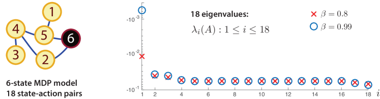
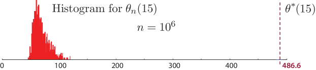
It is now known that the asymptotic covariance $\Sigma_{\text{\tiny$\Theta$}}$ appearing in (19a) is not finite if $\gamma>1/2$ [16, 17] (see also the sample complexity analysis that followed in [49]). A running example in this prior work and [34, 15, 13] is the stochastic-shortest-path problem whose state transition diagram is shown on the left hand side of Fig. 1. The state space ${\sf X}=\{1,\ldots,6\}$ coincides with the six nodes of the un-directed graph, and the action space is ${\sf U}=\{e_{x,x^{\prime}}\}$, $x,x^{\prime}\in{\sf X}$, indicating decisions on moves. Details on the description of disturbances can be found in [34, 15].

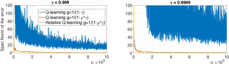
Fig. 2 shows results without the matrix gain. With $\gamma=0.8$ the output of the standard Q-learning algorithm is worthless after one million samples. The matrix gain does offer some benefit—see plots in the next section—but convergence remains very slow for $\gamma>{\mathchoice{\genfrac{}{}{}{1}{1}{2}}{\genfrac{}{}{}{1}{1}{2}}{\genfrac{}{}{}{3}{1}{2}}{\genfrac{}{}{}{3}{1}{2}}}$ using $\alpha_{n}=1/n$.

Refer to caption
Figure 2: Histogram of $10^{3}$ estimates of $\theta_{n}(15)$, with $n=10^{6}$ for the Watkins algorithm applied to the 6-state example with discount factor $\gamma=0.8$

ODE@$\infty$  Thm. 2.1 may be applied to Q-learning (4a) in this tabular setting, and the theorem easily extends to the case of the matrix gain algorithm (36).

It is clear that (SA1) holds, and (SA2) holds for oblivious training as assumed here. As already remarked, it is not difficult to establish stability of (37) to establish (SA3).

The ODE@$\infty$ associated with (37) is a minor modification:

$${\mathchoice{\genfrac{}{}{}{1}{d}{dt}}{\genfrac{}{}{}{1}{d}{dt}}{\genfrac{}{}{}{3}{d}{dt}}{\genfrac{}{}{}{3}{d}{dt}}}x_{t}=A(x_{t})x_{t}$$

We have ${\mathchoice{\genfrac{}{}{}{1}{d}{dt}}{\genfrac{}{}{}{1}{d}{dt}}{\genfrac{}{}{}{3}{d}{dt}}{\genfrac{}{}{}{3}{d}{dt}}}\|x_{t}\|_{\infty}\leq-(1-\gamma)\|x_{t}\|_{\infty}$, which implies that the ODE@$\infty$ is stable as required in Thm. 2.1.

3.3 Change your goals

Recall that the covariance $\Sigma_{\text{\tiny$\Theta$}}$ defined in (19a) is not finite for Q-learning in the form (36) with step-size $\alpha_{n}=g/n$ using $g<{\mathchoice{\genfrac{}{}{}{1}{1}{2}}{\genfrac{}{}{}{1}{1}{2}}{\genfrac{}{}{}{3}{1}{2}}{\genfrac{}{}{}{3}{1}{2}}}(1-\gamma)^{-1}$, which explains the poor performance illustrated in Fig. 2.

A reader with experience in SA would counter that this is a poor choice of step-size. Use instead $\alpha_{n}=1/n^{\rho}$, with $\rho\in({\mathchoice{\genfrac{}{}{}{1}{1}{2}}{\genfrac{}{}{}{1}{1}{2}}{\genfrac{}{}{}{3}{1}{2}}{\genfrac{}{}{}{3}{1}{2}}},1)$, and then average using (11) to obtain $\{\theta^{\text{\tiny\sf PR}}_{n}\}$. It is found that averaging fails for this example for large discount factors, even though it is known that these estimates achieve the optimal asymptotic covariance [34, 15, 13].

The observed numerical instability is a consequence of the eigenvalue at $-(1-\gamma)$ for $A^{*}$. This can be moved through a change in objective. For example, construct an algorithm that estimates the relative Q-function,

$$H^{\star}(x,u)=Q^{\star}(x,u)-\langle\upnu,Q^{\star}\rangle$$

where $\upnu$ is a fixed pmf on ${\sf X}\times{\sf U}$. Subtracting a constant doesn’t change the minimizer over $u$, and has enormous benefits.

The function $H^{\star}$ satisfies a DP equation similar to (8), which motivates relative Q-learning. It is shown in [18] that the eigenvalues of $A^{*}$ remain bounded away from the imaginary axis uniformly for all $0\leq\gamma\leq 1$, resulting in much faster convergence. See [34] for generalizations.

Fig. 3 is adapted from [18] for the six-state example. The plots show the span semi-norm error $\|Q^{\theta}-Q^{\star}\|_{S}$ for three algorithms, and two very large discount factors: $\gamma=0.999$ and $\gamma=0.9999$. The plots illustrate two important points:

1.  Q-learning with a smaller gain converges quickly to $Q^{*}$ when measured in the span norm

$$\|Q^{\theta}-Q^{\star}\|_{S}\mathbin{:=}\min_{a}\sup_{x,u}|Q^{\theta}(x,u)-Q^{\star}(x,u)|\,,\qquad\theta\in\mathbb{R}^{d}$$

2.  Convergence of relative Q-learning is very fast in this example, even with discount factor close to unity.

It appears that the span norm difference between estimates obtained using Q-learning and relative Q-learning is very small. This observation may be anticipated by comparing the respective mean flows [18].

Refer to caption
Figure 3: Plots of the span semi-norm of the error $Q^{\theta_{n}}-Q^{\star}$ for two versions of Q-learning distinguished by the step-size, and relative Q-learning.

4 Zap

Here the tabular setting is abandoned, and we do not even require linear function approximation. We maintain the assumption that the input for training is oblivious.

If our goal is to ensure that ${\widebar{f}}(\upvartheta_{t})\to 0$ as $t\to\infty$ then we should design dynamics to ensure this. One approach, the focus of Devraj’s dissertation [13] and a focus of the monograph [34], is the Newton-Raphson Flow:

$${\mathchoice{\genfrac{}{}{}{1}{d}{dt}}{\genfrac{}{}{}{1}{d}{dt}}{\genfrac{}{}{}{3}{d}{dt}}{\genfrac{}{}{}{3}{d}{dt}}}{\widebar{f}}(\upvartheta_{t})=-{\widebar{f}}(\upvartheta_{t})\quad\Longrightarrow\quad{\widebar{f}}(\upvartheta_{t})=e^{-t}{\widebar{f}}(\upvartheta_{0})$$ (39)

From the chain rule this results in the mean flow dynamics,

$${\mathchoice{\genfrac{}{}{}{1}{d}{dt}}{\genfrac{}{}{}{1}{d}{dt}}{\genfrac{}{}{}{3}{d}{dt}}{\genfrac{}{}{}{3}{d}{dt}}}\upvartheta_{t}=-G_{t}{\widebar{f}}(\upvartheta_{t})\,,\qquad G_{t}=A(\upvartheta_{t})^{-1}$$ (40)

where $A(\theta)$ is defined in (14).

Refer to caption
Figure 4: Simulation-based $2\sigma$ confidence intervals for the six Q-learning algorithms.

Zap stochastic approximation.  This is a two time-scale algorithm introduced in [16, 17]. For initialization $\theta_{0}\,\in\mathbb{R}^{d}$, and $\widehat{A}_{0}\in\mathbb{R}^{d\times d}$, obtain the sequence of estimates $\{\theta_{n}:n\geq 0\}$ recursively:

$\displaystyle\theta_{n+1}$ $\displaystyle=\theta_{n}-\alpha_{n+1}\widehat{A}_{n+1}^{-1}f(\theta_{n}\,,\Phi_{n+1})$ (41a)
$\displaystyle\widehat{A}_{n+1}$ $\displaystyle=\widehat{A}_{n}+\beta_{n+1}[A_{n+1}-\widehat{A}_{n}]\,,\qquad A_{n+1}\mathbin{:=}\partial_{\theta}f_{n+1}(\theta_{n})\,.$ (41b)

The two gain sequences $\{\alpha_{n}\}$ and $\{\beta_{n}\}$ satisfy (13).

The original motivation was to optimize the rate of convergence, which it does under mild assumptions using $\alpha_{n}=1/n$:

$$\Sigma_{\text{\tiny$\Theta$}}\mathbin{:=}\lim_{n\to\infty}n{\sf E}[{\tilde{\theta}}_{n}{{\tilde{\theta}}_{n}}^{\intercal}]=\Sigma^{\text{\tiny\sf PR}}_{\text{\tiny$\Theta$}}$$

This choice of gain $g$ is critical with the choice $\alpha_{n}=g/n$:

1.  $\Sigma_{\text{\tiny$\Theta$}}$ is finite when $g>{\mathchoice{\genfrac{}{}{}{1}{1}{2}}{\genfrac{}{}{}{1}{1}{2}}{\genfrac{}{}{}{3}{1}{2}}{\genfrac{}{}{}{3}{1}{2}}}$, but optimal only if $g=1$.

2.  $\hbox{\rm trace\,}(\Sigma_{\text{\tiny$\Theta$}})=\infty$ if $0<g<{\mathchoice{\genfrac{}{}{}{1}{1}{2}}{\genfrac{}{}{}{1}{1}{2}}{\genfrac{}{}{}{3}{1}{2}}{\genfrac{}{}{}{3}{1}{2}}}$ and $\Sigma_{\Delta}^{*}$ is full rank.

It was discovered in later research that the positive results hold even for nonlinear function approximation [11]. Hence the greatest value of the matrix gain is the creation of a universally stable algorithm.

Refer to caption
Figure 5: Histograms of the maximal Bellman error at iteration $n=10^{6}$.

In the applications to Q-learning considered here, the accuracy of a parameter estimate $\theta$ may be measured in terms of the Bellman error and its maximum

$\displaystyle{\cal B}^{\theta}(x,u)$ $\displaystyle=\theta(x,u)-r(x,u)-\beta\sum_{x^{\prime}\in{\sf X}}P_{u}(x,x^{\prime})\max_{u^{\prime}}\theta(x^{\prime},u^{\prime})$ (42a)
$\displaystyle\overline{\cal B}^{\theta}$ $\displaystyle=\max_{x,u}|{\cal B}^{\theta}(x,u)|$ (42b)

Given that the CLT holds for $\sqrt{n}{\tilde{\theta}}_{n}$, the sequence $\{\sqrt{n}\,\overline{\cal B}^{\theta_{n}}\}$ also converges in distribution as $n\to\infty$.

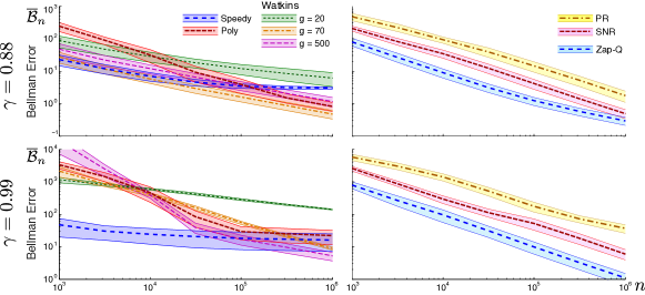
Fig. 4 is taken from [15] which contains full details on the experiments. Plots show the empirical mean and $2\sigma$ confidence intervals for $\gamma=0.8$ in row 1, and $\beta=0.99$ in row 2. The algorithms considered in the second column are explained here:

PR  Estimates obtained from Q-learning and averaging (36), with step-size $\alpha_{n}=1/n^{0.85}$.

SNR  The single time scale variant of Zap Q-learning using $\alpha_{n}=\beta_{n}=1/n$ (for which no theory is available).

Zap  Zap Q-learning using $\alpha_{n}=1/n$ and $\beta_{n}=1/n^{0.85}$.

Fig. 5 shows histograms of $\{\overline{\cal B}_{n}^{i},\,1\leq i\leq N\}$, $n=10^{6},$ for all the six algorithms; this corresponds to the data shown in Fig. 4 at $n=10^{6}$. Once again, full details may be found in [15].

5 Zap Zero

If we denote $w_{t}=G_{t}{\widebar{f}}(\upvartheta_{t})$ in the notation of (40), then equivalently $A(\upvartheta_{t})w_{t}-{\widebar{f}}(\upvartheta_{t})=0$ for all $t$. The Zap Zero algorithm of [34] is designed to achieve this constraint without matrix inversion. The ODE method for design suggests the $2d$-dimensional ODE

$\displaystyle{\mathchoice{\genfrac{}{}{}{1}{d}{dt}}{\genfrac{}{}{}{1}{d}{dt}}{\genfrac{}{}{}{3}{d}{dt}}{\genfrac{}{}{}{3}{d}{dt}}}\upvartheta_{t}$ $\displaystyle=-w_{t}$ (43)
$\displaystyle{\mathchoice{\genfrac{}{}{}{1}{d}{dt}}{\genfrac{}{}{}{1}{d}{dt}}{\genfrac{}{}{}{3}{d}{dt}}{\genfrac{}{}{}{3}{d}{dt}}}w_{t}$ $\displaystyle=\beta_{t}\bigl{[}A(\upvartheta_{t})w_{t}-{\widebar{f}}(\upvartheta_{t})\bigr{]}$

in which the time varying gain is introduced in anticipation of a two time-scale SA translation. The time inhomogeneous ODE (43) is stable provided $\beta_{t}\uparrow\infty$ as $t\to\infty$, and in addition (SA4) holds with $A(\theta)$ Hurwitz for each $\theta$.

A universally stable algorithm  A third state variable is introduced for reasons to be explained when we consider the SA translation. Fix $M>0$, an arbitrary positive definite matrix, and consider the ODE

$\displaystyle{\mathchoice{\genfrac{}{}{}{1}{d}{dt}}{\genfrac{}{}{}{1}{d}{dt}}{\genfrac{}{}{}{3}{d}{dt}}{\genfrac{}{}{}{3}{d}{dt}}}\upvartheta_{t}$ $\displaystyle=-[\upvartheta_{t}+z_{t}]$ (44)
$\displaystyle{\mathchoice{\genfrac{}{}{}{1}{d}{dt}}{\genfrac{}{}{}{1}{d}{dt}}{\genfrac{}{}{}{3}{d}{dt}}{\genfrac{}{}{}{3}{d}{dt}}}w_{t}$ $\displaystyle=-\beta_{t}\bigl{[}A(\upvartheta_{t})\{\upvartheta_{t}+z_{t}\}-{\widebar{f}}(\upvartheta_{t})\bigr{]}$
$\displaystyle{\mathchoice{\genfrac{}{}{}{1}{d}{dt}}{\genfrac{}{}{}{1}{d}{dt}}{\genfrac{}{}{}{3}{d}{dt}}{\genfrac{}{}{}{3}{d}{dt}}}z_{t}$ $\displaystyle=-\beta_{t}\bigl{[}z_{t}-L_{t}w_{t}\bigr{]}$ $\displaystyle L_{t}=MA(\upvartheta_{t})^{\intercal}$

The choice ${\mathchoice{\genfrac{}{}{}{1}{d}{dt}}{\genfrac{}{}{}{1}{d}{dt}}{\genfrac{}{}{}{3}{d}{dt}}{\genfrac{}{}{}{3}{d}{dt}}}z_{t}-\beta_{t}\bigl{[}z_{t}-MA(\upvartheta_{t})^{\intercal}w_{t}\bigr{]}$ is just one option. Alternatives are described in [23].

Assuming once more that $\beta_{t}\uparrow\infty$ as $t\to\infty$, singular perturbation theory (e.g. [22]) provides methodology for verification of stability of (44), proceeding in two steps:

1.  Consider the pair of ODEs with the slow variable frozen:

$\displaystyle{\mathchoice{\genfrac{}{}{}{1}{d}{dt}}{\genfrac{}{}{}{1}{d}{dt}}{\genfrac{}{}{}{3}{d}{dt}}{\genfrac{}{}{}{3}{d}{dt}}}w^{\theta}_{t}$ $\displaystyle=-A(\theta)\{\theta+z^{\theta}_{t}\}+{\widebar{f}}(\theta)$
$\displaystyle{\mathchoice{\genfrac{}{}{}{1}{d}{dt}}{\genfrac{}{}{}{1}{d}{dt}}{\genfrac{}{}{}{3}{d}{dt}}{\genfrac{}{}{}{3}{d}{dt}}}z^{\theta}_{t}$ $\displaystyle=-z^{\theta}_{t}+L(\theta)w^{\theta}_{t}$ $\displaystyle L(\theta)=MA(\theta)^{\intercal}$

The gain $\beta_{t}$ has been removed via a time transformation. For stability analysis it is more convenient to write,

$\displaystyle{\mathchoice{\genfrac{}{}{}{1}{d}{dt}}{\genfrac{}{}{}{1}{d}{dt}}{\genfrac{}{}{}{3}{d}{dt}}{\genfrac{}{}{}{3}{d}{dt}}}\begin{bmatrix}w^{\theta}_{t}\\ z^{\theta}_{t}\end{bmatrix}=\begin{bmatrix}0&-A(\theta)\\ MA(\theta)^{\intercal}&-I\end{bmatrix}\begin{bmatrix}w^{\theta}_{t}\\ z^{\theta}_{t}\end{bmatrix}+\begin{bmatrix}{\widebar{f}}(\theta)-A(\theta)\theta\\ 0\end{bmatrix}$ (45)

This is a linear system with constant input. It is stable because any eigenvalue $\lambda$ of the state matrix solves the equation

$$\lambda^{2}+\lambda+\mu_{+}=0$$

for some eigenvalue $\mu_{+}>0$ of the positive definite matrix $A(\theta)MA(\theta)^{\intercal}$. Any solution to this equation lies in the strict left half plane of $\mathbb{C}$.

The equilibrium $(w^{\theta}_{\infty};z^{\theta}_{\infty})$ of (45) satisfies

$$-A(\theta)\{\theta+z^{\theta}_{\infty}\}+{\widebar{f}}(\theta)=0\,,\qquad MA(\theta)^{\intercal}w^{\theta}_{\infty}-z^{\theta}_{\infty}=0\,.$$ (46)

2.  The equilibrium for (45) is substituted into the dynamics for the slow variable to obtain the approximation $x_{t}\approx\upvartheta_{t}$ with

$${\mathchoice{\genfrac{}{}{}{1}{d}{dt}}{\genfrac{}{}{}{1}{d}{dt}}{\genfrac{}{}{}{3}{d}{dt}}{\genfrac{}{}{}{3}{d}{dt}}}x_{t}=-[\theta+z_{\infty}^{\theta}]\big{|}_{\theta=x_{t}}$$

The equilibrium equations (46) imply that $\theta+z^{\theta}_{\infty}=[A(\theta)]^{-1}{\widebar{f}}(\theta)$ for all $\theta$, so that we recover the Newton-Raphson flow, ${\mathchoice{\genfrac{}{}{}{1}{d}{dt}}{\genfrac{}{}{}{1}{d}{dt}}{\genfrac{}{}{}{3}{d}{dt}}{\genfrac{}{}{}{3}{d}{dt}}}x_{t}=-[A(x_{t})]^{-1}{\widebar{f}}(x_{t})$.

SA Translation  The 2023 version of the Zap Zero SA algorithm is defined by the $3d$-dimensional recursion motivated by the ODE (44). For initialization $\theta_{0},w_{0},z_{0}\,\in\mathbb{R}^{d}$, obtain the sequence of estimates recursively:

$\displaystyle\theta_{n+1}$ $\displaystyle=\theta_{n}-\alpha_{n+1}\bigl{[}\theta_{n}+L_{n+1}w_{n}\bigr{]}$ (47a)
$\displaystyle w_{n+1}$ $\displaystyle=w_{n}-\beta_{n+1}\bigl{[}A_{n+1}\{\theta_{n}+z_{n}\}-f_{n+1}(\theta_{n})\bigr{]}$ (47b)
$\displaystyle z_{n+1}$ $\displaystyle=z_{n}-\beta_{n+1}\bigl{[}z_{n}-L_{n+1}w_{n}\bigr{]}$ $\displaystyle L_{n+1}=MA_{n+1}^{\intercal}$ (47c)

where as above $A_{n+1}\mathbin{:=}\partial_{\theta}f_{n+1}(\theta_{n})$. The two gain sequences $\{\alpha_{n}\}$ and $\{\beta_{n}\}$ satisfy (13).

Why is there a need for dimension $3d$?  Theory predicts that $z_{n}\approx MA(\theta_{n})^{\intercal}w_{n}$ for large $n$, which motivates elimination of $\{z_{n}\}$ to obtain,

$\displaystyle\theta_{n+1}$ $\displaystyle=\theta_{n}-\alpha_{n+1}\bigl{[}\theta_{n}+M\widehat{A}_{n+1}^{\intercal}w_{n}\bigr{]}$
$\displaystyle w_{n+1}$ $\displaystyle=w_{n}-\beta_{n+1}\bigl{[}\widehat{A}_{n+1}\{\theta_{n}+M\widehat{A}_{n+1}^{\intercal}w_{n}\}-f_{n+1}(\theta_{n})\bigr{]}$

A third recursion is required to construct the matrix sequence $\{\widehat{A}_{n+1}\}$, which is why (5) is a much simpler recursion.

The assumptions in the following are adapted from [11] in their treatment of Zap SA.

Theorem 5.1.

Suppose that the following hold:

(i)  Assumptions (SA1) and (SA2).

(ii)  The derivative (14) is a continuous function of $\theta$, satisfying ${\mathop{\rm det}}(A(\theta))\neq 0$ for all $\theta$.

(iii)  The function $\|{\widebar{f}}(\theta)\|$ is coercive: $\displaystyle\lim_{\|\theta\|\to\infty}\|{\widebar{f}}(\theta)\|=\infty$.

Then, there is a unique solution to ${\widebar{f}}(\theta^{*})={\mathchoice{{\mathchoice{\mbox{\large\sf 0}}{\mbox{\large\sf 0}}{\mbox{\tiny\sf 0}}{\mbox{\tiny\sf 0}}}}{\mbox{\sf 0}}{\mbox{\tiny\sf 0}}{\mbox{\tiny\sf 0}}}$, and the Zap Zero algorithm (5) is convergent for each initial condition:

$$\lim_{n\to\infty}\theta_{n}=\theta^{*}\,,\quad\lim_{n\to\infty}w_{n}=w^{*}_{\infty}\,,\quad\lim_{n\to\infty}z_{n}=z^{*}_{\infty}\qquad a.s.,$$

with $w^{*}_{\infty}=w^{\theta}_{\infty}$, $z^{*}_{\infty}=z^{\theta}_{\infty}$ evaluated at $\theta=\theta^{*}$.

Proof.

As in the Newton-Raphson flow, the coerciveness assumption is imposed to ensure that convergence ${\widebar{f}}(\upvartheta_{t})\to 0$ as $t\to\infty$, implies that $\{\upvartheta_{t}\}$ is bounded. We then conclude that any limit point is a root of ${\widebar{f}}$, and uniqueness of $\theta^{*}$ quickly follows. Convergence of (5) then follows from standard theory of two time-scale stochastic approximation [9].     $\sqcap$ $\sqcup$

Many generalizations are possible. In particular, it is shown in [11] that invertibility of $A(\theta)$ for all $\theta$ is not required, but may be replaced with the following: it is assumed that $A(\theta){\widebar{f}}(\theta)={\mathchoice{{\mathchoice{\mbox{\large\sf 0}}{\mbox{\large\sf 0}}{\mbox{\tiny\sf 0}}{\mbox{\tiny\sf 0}}}}{\mbox{\sf 0}}{\mbox{\tiny\sf 0}}{\mbox{\tiny\sf 0}}}$ holds only if ${\widebar{f}}(\theta)={\mathchoice{{\mathchoice{\mbox{\large\sf 0}}{\mbox{\large\sf 0}}{\mbox{\tiny\sf 0}}{\mbox{\tiny\sf 0}}}}{\mbox{\sf 0}}{\mbox{\tiny\sf 0}}{\mbox{\tiny\sf 0}}}$. This justifies a modification of the Newton-Raphson flow in which $A(\upvartheta_{t})^{-1}{\widebar{f}}(\upvartheta_{t})$ uses a pseudo-inverse when the matrix is not invertible. It is also shown in this prior work that $A$ need not be continuous in applications to Q-learning. Extending these generalizations to Zap Zero is a topic for research, but is not expected to be a big challenge.

Unfortunately we do not yet know how to verify all of the assumptions of Thm. 5.1 for Q-learning, in which ${\widebar{f}}$ defined in (34a), even in the relaxed form described in the previous paragraph. This means the existence of a solution to the projected Bellman equation remains an open topic of research when using oblivious training.

6 Stability with Optimism

The theory surveyed in the preceding section imposed oblivious training. In the case of Watkins’ Q-learning this assumption was imposed in part for historical reasons, though we will see that the analysis is somewhat more complex when we consider parameter dependent policies. The technical challenges for Zap Q-learning are far more interesting because the definition of the linearization $A(\theta)$ is not obvious. See the conclusions for further discussion.

We begin with a motivating example.

Refer to caption
Figure 6: Baird’s star example.

6.1 Baird’s star example
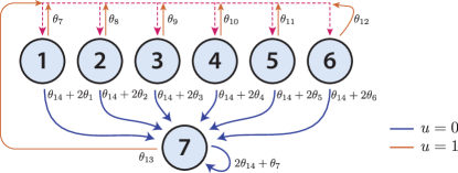
There are seven states ${\sf X}=\{1,\dots,7\}$ and two actions ${\sf U}=\{0,1\}$, in which $X_{k+1}=7$ with probability one whenever $U_{k}=0$. If $U_{k}=1$ then $X_{k+1}$ is uniformly distributed over states $\{1,\dots,6\}$.

In [4] it is assumed the cost is identically zero. We take $c(x,u)=0$ if $x\leq 6$ and $c(7,u)=-10$ (independent of $u$).

The Q-function is linearly parameterized with dimension $d=14$. A schematic is shown in Fig. 6, adapted from [4], indicating the following values of $Q^{\theta}(x,u)$:

$\bullet$  $\theta_{14}+2\theta_{x}$ when $(x,u)=(x,0)$, with $1\leq x\leq 6$.

$\bullet$  $2\theta_{14}+\theta_{7}$ when $(x,u)=(7,0)$.

$\bullet$  $\theta_{13}$ when $(x,u)=(7,1)$.

$\bullet$  $\theta_{6+x}$ when $(x,u)=(x,1)$, with $1\leq x\leq 6$.

We refer the reader to the source [4] (the final page contains a full description of the model considered in the experiments surveyed here), and [42] for a fuller discussion.

Refer to caption
Figure 7: Evolution of the Q-function approximations for two values of discount factor, and using an $\varepsilon$-greedy policy with common value of $\varepsilon=0.5$.

figure]f:TwoDiscBaird

The following oblivious policy is considered in [4]: $U_{k}=0$ with probability $1/7$, and otherwise $U_{k}=1$. While well-motivated from the point of view of exploration, it was shown that the parameter estimates diverge when the discount factor is sufficiently large.

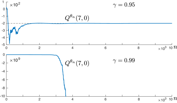
LABEL:f:TwoDiscBaird shows trajectories from the Q-learning algorithm (4a) with an $\varepsilon$-greedy policy using $\varepsilon=0.5$. The ideal behavior is that $Q^{\theta_{n}}(x,u)\to Q^{\star}(x,u)=-10/(1-\gamma)$ as $n\to\infty$ when $(x,u)=(7,0)$. The figure shows convergence when $\gamma=0.95$, but the parameters are divergent with discount factor $\gamma=0.99$.

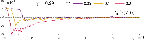
With the larger discount factor we obtain stability when using a smaller value of $\varepsilon>0$. LABEL:f:BigDiscBaird shows typical results for three small values. The dashed line indicates $Q^{*}(7,0)$.

The step-size sequence was taken to be $\alpha_{n}=\min(\bar{\alpha},g/n^{\rho})$ using $g=1/(1-\gamma)$, $\rho=0.85$, and $\bar{\alpha}=0.1$ in each run. See Section A.5 for Matlab code.

Refer to caption
Figure 8: Evolution of the Q-function approximations when using an $\varepsilon$-greedy policy. Convergence holds when $\varepsilon>0$ is sufficiently small.

figure]f:BigDiscBaird

See [18] for an explanation for slow convergence with a large discount factor, and for explanation of the choice $g=1/(1-\gamma)$. This prior work is based on consideration of the linearization matrix $A^{*}=A(\theta^{*})$ (see Lemma A.3 for a representation). LABEL:f:haA shows a plot of the maximum real part of $A^{*}$ as a function of $\varepsilon>0$, with $A^{*}$ estimated via Monte-Carlo. For larger values of $\varepsilon>0$ we see that $A^{*}$ is not Hurwitz for the three choices of discount factor. There is also trouble for very small $\varepsilon>0$: The discussion following Thm. 2.1 suggests that the asymptotic covariance will be very large when $\max(\text{Real}\,\lambda(A^{*}))$ is close to zero, but the covariance $\Sigma_{\Delta}^{*}$ must also be considered to make any conclusions.
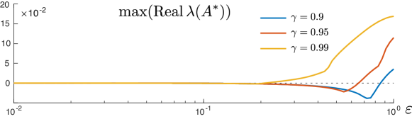
Refer to caption
Figure 9: The maximum eigenvalue of $A^{*}$ as a function of $\varepsilon$. The matrix is Hurwitz for sufficiently small $\varepsilon>0$, but some eigenvalues approach zero with vanishing $\varepsilon$.

figure]f:haA

6.2 Stability with linear function approximation

The main result of this section shows how exploration using a policy of the form (24) encourages stability of the Q-learning algorithm (4a). Analysis requires the family of autocorrelation matrices,

$\displaystyle R^{\text{\tiny$\Theta$}}(\theta)$ $\displaystyle={\sf E}_{\uppi_{\theta}}\bigl{[}\psi(X_{n},\upphi^{\theta}(X_{n}))\psi(X_{n},\upphi^{\theta}(X_{n}))^{\intercal}\bigr{]}\qquad R^{\text{\tiny$\mathcal{W}$}}(\theta)={\sf E}_{\uppi_{\theta}}\bigl{[}\psi(X_{n},\mathcal{W}_{n})\psi(X_{n},\mathcal{W}_{n})^{\intercal}\bigr{]}$ (48a)
$\displaystyle R(\theta)$ $\displaystyle={\sf E}_{\uppi_{\theta}}[\psi_{(n)}\psi_{(n)}^{\intercal}]=(1-\varepsilon)R^{\text{\tiny$\Theta$}}(\theta)+\varepsilon R^{\text{\tiny$\mathcal{W}$}}(\theta)$ (48b)
The expectations are in steady-state, with stationary pmf $\uppi_{\theta}$ induced by the randomized stationary policy with fixed parameter.

A special case is considered in the assumptions, in which we take $\varepsilon=1$, and the randomized policy is then denoted $\widetilde{\upphi}^{{\text{\tiny$\mathcal{W}$}}}$, giving $\widetilde{\upphi}^{{\text{\tiny$\mathcal{W}$}}}(\,\cdot\,\mid x)=\upnu_{\text{\tiny$\mathcal{W}$}}(u)$ for all $x,u$. The (assumed unique) invariant pmf is denoted $\uppi_{\text{\tiny$\mathcal{W}$}}$, and the autocorrelation matrix

$$R^{\text{\tiny$\mathcal{W}$}}={\sf E}_{\uppi_{\text{\tiny$\mathcal{W}$}}}\bigl{[}\psi(X_{n},\mathcal{W}_{n})\psi(X_{n},\mathcal{W}_{n})^{\intercal}\bigr{]}\,,\qquad\textit{using $U_{k}=\mathcal{W}_{k}$ for all $k$.}$$ (48c)

The following assumptions are required in the main results of this section:

(49a)
(49b)

We also require small $\varepsilon>0$ in specification of the policies. Denote

$$\varepsilon_{\gamma}\mathbin{:=}\frac{(1-\gamma)^{2}}{(1-\gamma)^{2}+\gamma^{2}}$$ (50)
Theorem 6.1.

Consider the Q-learning algorithm (4a) with linear function approximation, and training policy (24) defined using the tamed Gibbs policy (29). Suppose moreover that (6.2) holds.

Then, for any $\varepsilon\in(0,\varepsilon_{\gamma})$ there is $\kappa_{\varepsilon,\gamma}>0$ for which the following hold using the $(\varepsilon,\kappa_{0})$-tamed Gibbs policy, using $\kappa_{0}\geq\kappa_{\varepsilon,\gamma}$:

(i)  The parameter estimates $\{\theta_{n}\}$ are bounded: there is a fixed constant $B_{\text{\tiny$\Theta$}}$, independent of $\kappa_{0}\geq\kappa_{\varepsilon,\gamma}$, such that (18) holds with probability one from each initial condition.

(ii)  There exists at least one solution to the projected Bellman equation (5).

See Section 6.3 for an extension of (ii) to the $\varepsilon$-greedy policy.

To see why (i) is plausible, consider an algorithm approximating (4a), in which the minimum defining $\underline{Q}^{\theta_{n}}(X_{n+1})$ is replaced by substitution of the input used for training:

$\displaystyle\theta_{n+1}$ $\displaystyle=\theta_{n}+\alpha_{n+1}\widetilde{\mathcal{D}}_{n+1}\zeta_{n}\,.$ (51)
$\displaystyle\widetilde{\mathcal{D}}_{n+1}$ $\displaystyle=c_{n}-Q^{\theta_{n}}(X_{n},U_{n})+\gamma Q^{\theta_{n}}(X_{n+1},U^{-}_{n+1})$

in which $U_{n+1}^{-}$ is obtained by sampling from $\widetilde{\upphi}^{\theta}(\,\cdot\,\mid x)$ using $x=X_{n+1}$ and $\theta=\theta_{n}$. The use of a soft-minimum instead of the hard minimum $\underline{Q}^{\theta_{n}}(X_{n+1})$ is common in the RL literature [42].

Stability of the ODE@$\infty$ is then relatively easy, from which we obtain the following:

Proposition 6.2.

Consider the recursion (51) with linear function approximation, and training policy (24) defined as the $(\varepsilon,\kappa_{0})$-tamed Gibbs policy (29) with $\varepsilon\in(0,1)$ and $\kappa_{0}>0$. Suppose moreover that (6.2) holds. Then, we obtain the conclusions of Thm. 6.1:

(i)  The parameter estimates $\{\theta_{n}\}$ are bounded with probability one from each initial condition.

(ii)  There exists at least one solution $\theta^{*}$ to ${\widebar{f}}(\theta^{*})={\mathchoice{{\mathchoice{\mbox{\large\sf 0}}{\mbox{\large\sf 0}}{\mbox{\tiny\sf 0}}{\mbox{\tiny\sf 0}}}}{\mbox{\sf 0}}{\mbox{\tiny\sf 0}}{\mbox{\tiny\sf 0}}}$, with ${\widebar{f}}$ the mean flow for (51).

We proceed with the proof of Prop. 6.2. The proof of Thm. 6.1 is postponed to the Appendix.

The recursion (51) is similar to the sequence of fixed point equations,

$$\theta_{n+1}=\theta_{n}+\alpha_{n+1}\bigl{[}c_{n}-Q^{\theta_{n}}(X_{n},U_{n})+\gamma Q^{\theta_{n}}(X_{n+1},U_{n+1})\bigr{]}$$

In which $\{U_{n}\}$ is obtained from the tamed Gibbs policy (so that $U_{n+1}$ depends on $\theta_{n+1}$). Assuming there is a solution for each $n$, this recursion and (51) share the same mean-flow vector fields.

The sequence of fixed point equations may be expressed in a form similar to the TD(0) learning algorithm,

$$\theta_{n+1}=\theta_{n}+\alpha_{n+1}\bigl{[}\psi_{(n)}c_{n}-\psi_{(n)}\{\psi_{(n)}-\gamma\psi_{(n+1)}\}^{\intercal}\theta_{n}\bigr{]}$$ (52)

This motivates consideration of the family of autocorrelation matrices

$$R_{k}(\theta)={\sf E}_{\uppi_{\theta}}[\psi_{(n+k)}\psi_{(n)}^{\intercal}]\,,\quad n,k\geq 0\,,$$

so that $R_{0}(\theta)=R(\theta)$ in the notation (48b).

The vector field for the mean flow associated with (51) is Lipschitz continuous and has an attractive form.

Lemma 6.3.

Under the assumptions of Prop. 6.2,

(i)  The vector field for the mean flow is

$${\widebar{f}}(\theta)=A(\theta)\theta-b(\theta)\,,\quad\textit{ in which $b(\theta)=-{\sf E}_{\uppi_{\theta}}[\psi_{(n)}c_{n}]$ and $A(\theta)=-R_{0}(\theta)+\gamma R_{-1}(\theta)$. }$$

(ii)  The limit defining ${\widebar{f}}_{\infty}$ in (16) exists and may be expressed

$${\widebar{f}}_{\infty}(\theta)=A_{\infty}(\theta)\theta\,,\qquad\textit{where}\quad A_{\infty}(\theta)=A(\theta/\|\theta\|)\quad\textit{for $\theta\neq{\mathchoice{{\mathchoice{\mbox{\large\sf 0}}{\mbox{\large\sf 0}}{\mbox{\tiny\sf 0}}{\mbox{\tiny\sf 0}}}}{\mbox{\sf 0}}{\mbox{\tiny\sf 0}}{\mbox{\tiny\sf 0}}}$.}$$
Proof.

Identification of ${\widebar{f}}$ follows immediately from (52) since $\theta$ is held fixed in the definition of the mean flow. The representation of the ODE@$\infty$ follows from structure of the policy highlighted in (31), which implies

$$\uppi_{r\theta}=\uppi_{\theta}\,,\quad A(r\theta)=A(\theta)\,,\quad\textit{and}\quad b(r\theta)=b(\theta)\qquad\textit{for all $r\geq 1$ when $\|\theta\|\geq 1$.}$$

$\sqcap$ $\sqcup$

Lemma 6.4.

Suppose that (49a) holds. Then, for the recursion (51) there exists $\delta_{\psi}>0$, independent of $\theta$ such that

$\displaystyle R_{0}(\theta)$ $\displaystyle\geq\delta_{\psi}I$ for all $\theta\in\mathbb{R}^{d}$
$\displaystyle\theta^{\intercal}A(\theta)\theta$ $\displaystyle\leq-(1-\gamma)\delta_{\psi}$ for all $\theta\in\mathbb{R}^{d}$, $\|\theta\|\geq 1$.
Proof.

The proof of the lower bound on $R_{0}(\theta)$ is identical to the proof of Lemma A.1 in the Appendix. From Lemma 6.3 (i) we have for $\theta\in\mathbb{R}^{d}$ satisfying $\|\theta\|\geq 1$,

$$\theta^{\intercal}A(\theta)\theta=-\theta^{\intercal}R_{0}(\theta)\theta+\gamma\theta^{\intercal}R_{-1}(\theta)\theta\leq-(1-\gamma)\theta^{\intercal}R_{0}(\theta)\theta\leq-(1-\gamma)\delta_{\psi}\|\theta\|^{2}$$

$\sqcap$ $\sqcup$

Proof of Prop. 6.2.

Let $V_{1}(\theta)={\mathchoice{\genfrac{}{}{}{1}{1}{2}}{\genfrac{}{}{}{1}{1}{2}}{\genfrac{}{}{}{3}{1}{2}}{\genfrac{}{}{}{3}{1}{2}}}\|\theta\|^{2}$ and apply Lemmas 6.3 and 6.4 to obtain, whenever $\|\upvartheta_{t}\|\geq 1$,

$${\mathchoice{\genfrac{}{}{}{1}{d}{dt}}{\genfrac{}{}{}{1}{d}{dt}}{\genfrac{}{}{}{3}{d}{dt}}{\genfrac{}{}{}{3}{d}{dt}}}V_{1}(\upvartheta_{t})=\upvartheta_{t}^{\intercal}{\widebar{f}}(\upvartheta_{t})=\upvartheta_{t}^{\intercal}\{A(\upvartheta_{t})\upvartheta_{t}-b(\upvartheta_{t})\}\leq-\delta_{1}\|\upvartheta_{t}\|^{2}+\|\upvartheta_{t}\|\|b(\upvartheta_{t})\|$$

with $\delta_{1}=(1-\gamma)\delta_{\psi}$. This gives, with $\bar{b}=\sup_{\theta}\|b(\theta)\|<\infty$,

$${\mathchoice{\genfrac{}{}{}{1}{d}{dt}}{\genfrac{}{}{}{1}{d}{dt}}{\genfrac{}{}{}{3}{d}{dt}}{\genfrac{}{}{}{3}{d}{dt}}}V_{1}(\upvartheta_{t})\leq-{\mathchoice{\genfrac{}{}{}{1}{1}{2}}{\genfrac{}{}{}{1}{1}{2}}{\genfrac{}{}{}{3}{1}{2}}{\genfrac{}{}{}{3}{1}{2}}}\delta_{1}\|\upvartheta_{t}\|^{2}\,,\qquad\|\upvartheta_{t}\|\geq\max(1,2\bar{b})$$

We then obtain (v4) using $V(\theta)=\sqrt{V(\theta)}=\|\theta\|$ for $\|\theta\|\geq\max(1,2\bar{b})$ (modified in a neighborhood of the origin to impose the $C^{1}$ condition):

$${\mathchoice{\genfrac{}{}{}{1}{d}{dt}}{\genfrac{}{}{}{1}{d}{dt}}{\genfrac{}{}{}{3}{d}{dt}}{\genfrac{}{}{}{3}{d}{dt}}}V(\upvartheta_{t})\leq-\delta_{v}V(\upvartheta_{t})\,,\qquad\|\upvartheta_{t}\|\geq\max(1,2\bar{b})\,,\quad\textit{with $\delta_{v}=\delta_{1}/4$. }$$

Part (i) then follows from Thm. 2.1 (i) and part (ii) from Prop. 2.2.     $\sqcap$ $\sqcup$

6.3 Implications to the $\varepsilon$-greedy policy

A full analysis of Q-learning using the $\varepsilon$-greedy policy for training is beyond the scope of this paper due to discontinuity of the vector field. We find here that Thm. 6.1 admits a partial extension.

We consider here the corresponding mean flow (34c), and also the algorithm with matrix gain, whose mean flow vector field is

$$\bar{f}^{\textup{{zap}}}(\theta)=-\theta+[A(\theta)]^{-1}b(\theta)\,,\quad\theta\in\mathcal{C}^{\text{\tiny$\Theta$}}$$

This defines the dynamics expected when using Zap Q-learning based on (4).

The set $\mathcal{C}^{\text{\tiny$\Theta$}}$ defined in (23) may be expressed as the disjoint union,

$$\mathcal{C}^{\text{\tiny$\Theta$}}=\bigcup_{i}\mathcal{C}^{\text{\tiny$\Theta$}}_{i}$$

in which each $\mathcal{C}^{\text{\tiny$\Theta$}}_{i}$ is an open convex polyhedron, with $\upphi^{\theta}=\upphi^{\theta^{\prime}}$ for all $\theta,\theta^{\prime}\in\mathcal{C}^{\text{\tiny$\Theta$}}_{i}$. Consequently, both ${\widebar{f}}$ and $\bar{f}^{\textup{{zap}}}$ are constant on each set $\mathcal{C}^{\text{\tiny$\Theta$}}_{i}$.

For each $\theta\in\mathbb{R}^{d}$, denote by $\Upphi^{\theta}$ the set of all randomized $Q^{\theta}$-greedy policies: if $\widetilde{\upphi}\in\Upphi^{\theta}$ then

$$\sum_{u}\widetilde{\upphi}(u\mid x)Q^{\theta}(x,u)=\underline{Q}^{\theta}(x)\,,\qquad x\in{\sf X}\,.$$

If $\theta\in\mathcal{C}^{\text{\tiny$\Theta$}}$ then $\Upphi^{\theta}=\{\upphi^{\theta}\}$ is a singleton.

Theorem 6.5.

Suppose that (49a) holds. Then, the following hold for the mean flows associated with the Q-learning algorithm with $\varepsilon$-greedy training, provided $0<\varepsilon<\varepsilon_{\gamma}$:

(i)  There exists $\theta^{*}\in\mathbb{R}^{d}$ and $\widetilde{\upphi}^{*}\in\Upphi^{\theta^{*}}$ such that ${\widebar{f}}(\theta^{*})={\mathchoice{{\mathchoice{\mbox{\large\sf 0}}{\mbox{\large\sf 0}}{\mbox{\tiny\sf 0}}{\mbox{\tiny\sf 0}}}}{\mbox{\sf 0}}{\mbox{\tiny\sf 0}}{\mbox{\tiny\sf 0}}}$, with ${\widebar{f}}$ defined in (34c) in which the expectation is taken in steady-state using $\uppi_{\theta^{*}}$ obtained from the randomized policy,

$$\widetilde{\upphi}^{\theta^{*}}(u\mid x)=(1-\varepsilon)\widetilde{\upphi}^{*}(u\mid x)+\varepsilon\upnu_{\text{\tiny$\mathcal{W}$}}(u)$$ (53)

(ii)  If $\theta^{*}\in\mathcal{C}^{\text{\tiny$\Theta$}}$ then $\theta^{*}$ is locally asymptotically stable for the mean flow with vector field ${\widebar{f}}$.

(iii)  If $\theta^{*}\in\mathcal{C}^{\text{\tiny$\Theta$}}_{i}$ for some $i$, then $\theta^{*}$ is locally asymptotically stable for the mean flow with vector field $\bar{f}^{\textup{{zap}}}$, with domain of attraction including all of $\mathcal{C}^{\text{\tiny$\Theta$}}_{i}$.

Proof.

The proof of (i) is contained in Section A.4.

If ${\widebar{f}}(\theta^{*})=0$ with $\theta^{*}\in\mathcal{C}^{\text{\tiny$\Theta$}}$, it then follows from the definition of the vector field that $\theta^{*}=[A(\theta^{*})]^{-1}b(\theta^{*})$. Consequently, for $\theta$ in a neighborhood of $\theta^{*}$ contained in $\mathcal{C}^{\text{\tiny$\Theta$}}$,

$${\widebar{f}}(\theta)=A(\theta^{*})\bigl{(}\theta-\theta^{*}\bigr{)}$$

See Prop. A.4 for a proof that $A(\theta^{*})$ is Hurwitz, so that $\theta^{*}$ is locally asymptotically stable as claimed in (ii).

We have under the assumptions of (iii),

$$\bar{f}^{\textup{{zap}}}(\theta)=-\theta+\theta^{*}\,,\quad\theta\in\mathcal{C}^{\text{\tiny$\Theta$}}_{i}$$

If $\upvartheta_{0}\in\mathcal{C}^{\text{\tiny$\Theta$}}_{i}$ it follows that the solution to ${\mathchoice{\genfrac{}{}{}{1}{d}{dt}}{\genfrac{}{}{}{1}{d}{dt}}{\genfrac{}{}{}{3}{d}{dt}}{\genfrac{}{}{}{3}{d}{dt}}}\upvartheta_{t}=\bar{f}^{\textup{{zap}}}(\upvartheta_{t})$ is given by

$$\upvartheta_{t}=\theta^{*}+[\upvartheta_{t}-\theta^{*}]e^{-t}$$

Convexity of $\mathcal{C}^{\text{\tiny$\Theta$}}_{i}$ ensures that $\upvartheta_{t}\in\mathcal{C}^{\text{\tiny$\Theta$}}_{i}$ for all $t$, which completes the proof of (iii).     $\sqcap$ $\sqcup$

7 Conclusions and Thoughts for the Future

This article began as a companion to the INFORMS APS lecture delivered by the author in June, 2023. The scope of the lecture and this article grew to include several significant new contributions, which invite many avenues for future research:

1.  The new Zap Zero SA algorithm (5) is only one possible approach to approximate the Newton-Raphson flow. There may be approaches based on momentum—it will be worthwhile revisiting the NESA algorithm of [14].

2.  We now know that the existence of a solution to the projected Bellman equation exists under mild conditions, most important of which involves the choice of policy for training.

3.  The extension to average cost optimal control will be possible through consideration of [1]. And for the discounted case, better algorithms and better bounds on $\varepsilon$ might be obtained by adopting relative Q-learning algorithms [18, 34].

4.  We should consider other paradigms for algorithm design. The recent approaches [32, 5, 26, 27] are based on the linear programming formulation of optimal control due to of Manne, 1960 [29].

5.  Challenge with Zap. Based on theory surrounding the Actor-Critic method, we have for a policy of the form (25),

$$\partial_{\theta}{\widebar{f}}\,(\theta)={\sf E}_{\uppi_{\theta}}[A_{n}(\theta)]+{\sf E}_{\uppi_{\theta}}[{\hat{f}}_{n}\,(\theta)\Lambda_{n}(\theta)^{\intercal}]$$ (54)

in which $A_{n}(\theta)=\partial_{\theta}f_{n}\,(\theta)$. The expectations are in steady state under $\uppi_{\theta}$ (recall discussion surrounding (33)).

The second expectation involves the score function associated with the randomized policy,

$$\Lambda_{n}(\theta)=\nabla_{\theta}\log\widetilde{\upphi}^{\theta}(u\mid x)\Big{|}_{u=U_{n}\,,\ x=X_{n}}$$

The function ${\hat{f}}_{n}$ solves a certain Poisson equation. If the transition matrix $T_{\theta}$ is aperiodic, then for a stationary realization of $\{X_{n},U_{n}:n\geq 0\}$ we have

$${\sf E}_{\uppi_{\theta}}[{\hat{f}}_{n}(\theta)\Lambda_{n}(\theta)^{\intercal}]=\sum_{k=0}^{\infty}{\sf E}_{\uppi_{\theta}}[[f_{n-k}(\theta)-{\widebar{f}}(\theta)]\Lambda_{n}(\theta)^{\intercal}]$$

Based on this representation we can obtain unbiased estimates of $\partial_{\theta}{\widebar{f}}\,(\theta_{n})$ by adopting concepts from actor-critic algorithms. See [34, Ch. 10] for a survey in the style of this paper.

Analysis of the resulting algorithms will be considered in future research.

Appendix

Appendix A Stability with Optimism

This section concerns analysis of Q-learning with optimistic training, so that the input is defined by a randomized policy $\widetilde{\upphi}^{\theta}$. When $\theta$ is frozen, so that $U_{k}\sim\widetilde{\upphi}^{\theta}(\,\cdot\,\mid X_{k})$ for each $k$, then $X$ is a time homogeneous Markov chain with transition matrix,

$$P_{\theta}(x,x^{\prime})\mathbin{:=}\sum_{u}\widetilde{\upphi}^{\theta}(u\mid x)P_{u}(x,x^{\prime})\,,\qquad x,x^{\prime}\in{\sf X}\,.$$ (55)

Recall that in this case the joint process $\{(X_{k},U_{k}):k\geq 0\}$ is also Markovian, with transition matrix given in (33). We maintain the notation $\uppi_{\theta}$ for the unique invariant pmf for $T_{\theta}$.

Of course, the parameter $\theta$ is never frozen in any algorithm. The transition matrices $P_{\theta}$ and $T_{\theta}$ are introduced for analysis.

It is assumed that the function class is linear, $\{Q^{\theta}=\theta^{\intercal}\psi:\theta\in\mathbb{R}^{d}\}$ with $\psi\colon{\sf X}\times{\sf U}\to\mathbb{R}^{d}$.

A.1 A truly oblivious policy

We require structure of the truly oblivious policy defined by $U_{k}\equiv\mathcal{W}_{k}$ in the definition of $R^{\text{\tiny$\mathcal{W}$}}$ in (48c). The transition matrix for the joint process $\{(X_{k},U_{k}):k\geq 0\}$ can be obtained from (33), and is denoted

$$T_{\text{\tiny$\mathcal{W}$}}(z,z^{\prime})=P_{u}(x,x^{\prime})\upnu_{\text{\tiny$\mathcal{W}$}}(u^{\prime})\,,\qquad z=(x,u)\,,\ z^{\prime}=(x^{\prime},u^{\prime})\in{\sf X}\times{\sf U}\,.$$

The invariance equation $\uppi_{\text{\tiny$\mathcal{W}$}}(z^{\prime})=\sum_{z}\uppi_{\text{\tiny$\mathcal{W}$}}(z)T_{\theta}(z,z^{\prime})$ implies that the invariant pmf is product form:

$$\uppi_{\text{\tiny$\mathcal{W}$}}(z^{\prime})=\upmu_{\text{\tiny$\mathcal{W}$}}(x^{\prime})\upnu_{\text{\tiny$\mathcal{W}$}}(u^{\prime})\,,\qquad z^{\prime}=(x^{\prime},u^{\prime})\in{\sf X}\times{\sf U}\,.$$

in which $\upmu_{\text{\tiny$\mathcal{W}$}}(x^{\prime})=\sum_{u}\uppi_{\text{\tiny$\mathcal{W}$}}(x^{\prime},u)$ is the steady-state marginal distribution of $X$ under this policy. Similar notation is adopted for each of the invariant pmfs,

$$\upmu_{\theta}(x)=\sum_{u}\uppi_{\theta}(x,u)\,,\qquad x\in{\sf X}\,,\ \theta\in\mathbb{R}^{d}\,.$$

These are the invariant pmfs for $\{P_{\theta}\}$ appearing in (55).

Lemma A.1.

Suppose that the Markov chain with transition matrix $T_{\text{\tiny$\mathcal{W}$}}$ is uni-chain, so that $\uppi_{\text{\tiny$\mathcal{W}$}}$ is the unique invariant pmf. Consider any one of the three choices of $\{{\cal U}_{k}\}$ used in (24) with $\varepsilon<1$ and any choice of $\kappa$ in the case of (27) or $\{\kappa_{\theta}\}$ in the case of (29). The following conclusions then hold:

(i)  $T_{\theta}$ is also uni-chain, so that $\uppi_{\theta}$ is unique for any $\theta$.

(ii)  There is a constant $\delta_{\bullet}>0$ such that $\uppi_{\theta}(z)\geq\delta_{\bullet}\uppi_{\text{\tiny$\mathcal{W}$}}(z)$ for all $z$ and $\theta$. The constant $\delta_{\bullet}$ may depend on the policy parameters, but not $\theta$.

(iii)  $\uppi_{\theta}(x,u)\geq\varepsilon\upmu_{\theta}(x)\upnu_{\text{\tiny$\mathcal{W}$}}(u)$ for all $x,u$, and $\theta$.

(iv)  $R^{\text{\tiny$\mathcal{W}$}}(\theta)\geq\delta_{\bullet}R^{\text{\tiny$\mathcal{W}$}}$ for all $\theta\in\mathbb{R}^{d}$.

Proof.

Let ${\sf X}_{0}$ denote the support of $\upmu_{\text{\tiny$\mathcal{W}$}}$ and ${\sf U}_{0}$ denote the support of $\upnu_{\text{\tiny$\mathcal{W}$}}$. The uni-chain assumption is equivalent to the following reachability criterion: there is $N\geq 1$ and $\delta_{N}>0$ such that

$$\sum_{k=1}^{N}T^{k}_{\text{\tiny$\mathcal{W}$}}(z,z^{\prime})\geq\delta_{N}\,,\qquad\textit{for any $z\in{\sf X}\times{\sf U}$, and $z^{\prime}\in{\sf X}_{0}\times{\sf U}_{0}$,}$$

with $T^{k}_{\text{\tiny$\mathcal{W}$}}$ the $k$-step transition matrix. This is a version of Doeblin’s minorization condition that implies uniform ergodicity when the chain is aperiodic [37].

In view of (24) we have for any $\theta$,

$$\sum_{k=1}^{N}T^{k}_{\theta}(z,z^{\prime})\geq\sum_{k=1}^{N}\varepsilon^{k}T^{k}_{\text{\tiny$\mathcal{W}$}}(z,z^{\prime})\geq\varepsilon^{N}\delta_{N}\,,\qquad\textit{for any $z\in{\sf X}\times{\sf U}$, and $z^{\prime}\in{\sf X}_{0}\times{\sf U}_{0}$,}$$

Hence the family $\{T_{\theta}:\theta\in\mathbb{R}^{d}\}$ satisfies a uniform Doeblin minorization. In particular, each transition matrix is uni-chain, which establishes (i).

Part (ii) follows from the bounds above and invariance:

$$\uppi_{\theta}(z^{\prime})=\sum_{z}\uppi_{\theta}(z)\Bigl{(}\frac{1}{N}\sum_{k=1}^{N}T^{k}_{\theta}(z,z^{\prime})\Bigr{)}\geq\frac{1}{N}\varepsilon^{N}\delta_{N}\,,\qquad z^{\prime}\in{\sf X}_{0}\times{\sf U}_{0}$$

Part (iii) also follows from invariance in the following one-step form: we have from (33), and using the bound $\widetilde{\upphi}^{\theta}(u^{\prime}\mid x^{\prime})\geq\varepsilon\upnu_{\text{\tiny$\mathcal{W}$}}(u^{\prime})$,

$\displaystyle\uppi_{\theta}(z^{\prime})=\sum_{z}\uppi_{\theta}(z)T_{\theta}(z,z^{\prime})$ $\displaystyle=\sum_{x,u}\uppi_{\theta}(x,u)P_{u}(x,x^{\prime})\widetilde{\upphi}^{\theta}(u^{\prime}\mid x^{\prime})$
$\displaystyle\geq\varepsilon\sum_{x,u}\uppi_{\theta}(x,u)P_{u}(x,x^{\prime})\upnu_{\text{\tiny$\mathcal{W}$}}(u^{\prime})$
$\displaystyle=\varepsilon\upmu_{\theta}(x^{\prime})\upnu_{\text{\tiny$\mathcal{W}$}}(u^{\prime})$

For part (iv) consider the definition (48a), which gives

$$R^{\text{\tiny$\mathcal{W}$}}(\theta)=\sum_{x,u}\upmu_{\theta}(x)\upnu_{\text{\tiny$\mathcal{W}$}}(u)\psi(x,u)\psi(x,u)^{\intercal}$$

Applying (ii) gives $\upmu_{\theta}(x)\geq\delta_{\bullet}\upmu_{\text{\tiny$\mathcal{W}$}}(x)$ for all $x$, and hence the desired bound:

$$R^{\text{\tiny$\mathcal{W}$}}(\theta)\geq\delta_{\bullet}\sum_{x,u}\upmu_{\text{\tiny$\mathcal{W}$}}(x)\upnu_{\text{\tiny$\mathcal{W}$}}(u)\psi(x,u)\psi(x,u)^{\intercal}=\delta_{\bullet}R^{\text{\tiny$\mathcal{W}$}}\,$$

$\sqcap$ $\sqcup$

A.2 Mean flow for the $\varepsilon$-greedy policy

In this subsection the input is chosen to be the $\varepsilon$-greedy policy (24). The motivation is in part the fact that establishing stability of the ODE@$\infty$ in this case is far easier than the tamed Gibbs approximation.

The transition matrix (33) becomes

$$T_{\theta}(z,z^{\prime})=P_{u}(x,x^{\prime})\bigl{\{}(1-\varepsilon)\mathbb{I}\{u^{\prime}=\phi^{\theta}(x^{\prime})\}+\varepsilon\nu^{\text{\tiny$\mathcal{W}$}}(u^{\prime})\bigr{\}}\,,\qquad z=(x,u)\,,\ z^{\prime}=(x^{\prime},u^{\prime})\in{\sf X}\times{\sf U}\,.$$ (56)

The family $\{T_{\theta}:\theta\in\mathbb{R}^{d}\}$ is finite because there are only a finite number of deterministic stationary policies; it takes on a constant value on each connected component of $\mathcal{C}^{\text{\tiny$\Theta$}}$ (recall (23)).

Compact representations of $f$ and ${\widebar{f}}$ are obtained with additional notation. For $n\geq 0$ denote

$\displaystyle\psi_{(n)}^{\text{\tiny$\Theta$}}$ $\displaystyle=\psi(X_{n},\upphi^{\theta_{n}}(X_{n}))\quad$ $\displaystyle\psi_{(n)}^{\text{\tiny$\mathcal{W}$}}$ $\displaystyle=\psi(X_{n},\mathcal{W}_{n})$ (57)
$\displaystyle c^{\text{\tiny$\Theta$}}_{n}$ $\displaystyle=c(X_{n},\upphi^{\theta_{n}}(X_{n}))$ $\displaystyle c^{\text{\tiny$\mathcal{W}$}}_{n}$ $\displaystyle=c(X_{n},\mathcal{W}_{n})$

We have under the $\varepsilon$-greedy policy (24, 26),

$\displaystyle f_{n+1}(\theta_{n})=(1-B_{n})$ $\displaystyle\bigl{(}c^{\text{\tiny$\Theta$}}_{n}+\bigl{[}\gamma\psi_{(n+1)}^{\text{\tiny$\Theta$}}-\psi_{(n)}^{\text{\tiny$\Theta$}}\bigr{]}^{\intercal}\theta_{n}\bigr{)}\psi_{(n)}^{\text{\tiny$\Theta$}}$ (58)
$\displaystyle{}+B_{n}$ $\displaystyle\bigl{(}c^{\text{\tiny$\mathcal{W}$}}_{n}+\bigl{[}\gamma\psi_{(n+1)}^{\text{\tiny$\Theta$}}-\psi^{\text{\tiny$\mathcal{W}$}}_{n}\bigr{]}^{\intercal}\theta_{n}\bigr{)}\psi_{(n)}^{\text{\tiny$\mathcal{W}$}}$
Lemma A.2.

$\displaystyle{\sf E}_{\uppi_{\theta}}\bigl{[}\psi_{(n)}\{\psi_{(n+1)}^{\text{\tiny$\Theta$}}\}^{\intercal}\bigr{]}=R_{-1}(\theta)+\varepsilon D(\theta)$, in which

$$D(\theta)={\sf E}_{\uppi_{\theta}}\bigl{[}\psi_{(n)}\{\psi_{(n+1)}^{\text{\tiny$\Theta$}}-\psi_{(n+1)}^{\text{\tiny$\mathcal{W}$}}\}^{\intercal}\bigr{]}$$ (59)
Proof.

Starting with the definition $R_{-1}(\theta)={\sf E}_{\uppi_{\theta}}\bigl{[}\psi_{(n)}\{\psi_{(n+1)}\}^{\intercal}\bigr{]}$, we have under the $\varepsilon$-greedy policy,

$\displaystyle R_{-1}(\theta)$ $\displaystyle=(1-\varepsilon){\sf E}_{\uppi_{\theta}}\bigl{[}\psi_{(n)}\{\psi_{(n+1)}^{\text{\tiny$\Theta$}}\}^{\intercal}\bigr{]}+\varepsilon{\sf E}_{\uppi_{\theta}}\bigl{[}\psi_{(n)}\{\psi_{(n+1)}^{\text{\tiny$\mathcal{W}$}}\}^{\intercal}\bigr{]}$
$\displaystyle={\sf E}_{\uppi_{\theta}}\bigl{[}\psi_{(n)}\{\psi_{(n+1)}^{\text{\tiny$\Theta$}}\}^{\intercal}\bigr{]}+\varepsilon{\sf E}_{\uppi_{\theta}}\bigl{[}\psi_{(n)}\{\psi_{(n+1)}^{\text{\tiny$\mathcal{W}$}}-\psi_{(n+1)}^{\text{\tiny$\Theta$}}\}^{\intercal}\bigr{]}$

$\sqcap$ $\sqcup$

Lemma A.3.

The vector fields for the mean flow and the ODE@$\infty$ for the $\varepsilon$-greedy policy are

$\displaystyle{\widebar{f}}(\theta)=A(\theta)\theta$ $\displaystyle-b(\theta)\qquad\qquad{\widebar{f}}_{\infty}(\theta)=A(\theta)\theta$ (60a)
$\displaystyle\textit{ in which }\quad A(\theta)$ $\displaystyle=-\bigl{[}R_{0}(\theta)-\gamma R_{-1}(\theta)\bigr{]}+\varepsilon\gamma D(\theta)$ (60b)
$\displaystyle b(\theta)$ $\displaystyle=(1-\varepsilon)b^{\text{\tiny$\Theta$}}(\theta)+\varepsilon b^{\text{\tiny$\mathcal{W}$}}(\theta)$ (60c)

$b^{\text{\tiny$\Theta$}}(\theta)=-{\sf E}_{\uppi_{\theta}}[\psi_{(n)}^{\text{\tiny$\Theta$}}c_{n}^{\text{\tiny$\Theta$}}]$ and $b^{\text{\tiny$\mathcal{W}$}}(\theta)=-{\sf E}_{\uppi_{\theta}}[\psi_{(n)}^{\text{\tiny$\mathcal{W}$}}c(X_{n},\mathcal{W}_{n})]$.

Proof.

The representation (58) is equivalently expressed $f_{n+1}(\theta_{n})=A_{n+1}\theta_{n}-b_{n+1}$, in which

$\displaystyle A_{n+1}$ $\displaystyle=\psi_{(n)}\bigl{[}\gamma\psi_{(n+1)}^{\text{\tiny$\Theta$}}-\psi_{(n)}\bigr{]}^{\intercal}$
$\displaystyle b_{n+1}$ $\displaystyle=(1-B_{n})\psi_{(n)}^{\text{\tiny$\Theta$}}c(X_{n},\upphi^{\theta}(X_{n}))+B_{n}\psi_{(n)}^{\text{\tiny$\mathcal{W}$}}c(X_{n},\mathcal{W}_{n})$

The expression for $b(\theta)$ in the expression ${\widebar{f}}(\theta)={\sf E}_{\uppi_{\theta}}[f_{n+1}(\theta)=A(\theta)\theta-b(\theta)$ is immediate.

We have $A(\theta)=-R_{0}(\theta)+\gamma{\sf E}_{\uppi_{\theta}}\bigl{[}\psi_{(n)}\{\psi_{(n+1)}^{\text{\tiny$\Theta$}}\}^{\intercal}\bigr{]}$, so that (60b) follows from Lemma A.2.

The expression for ${\widebar{f}}_{\infty}$ follows from the fact that $A$ and $b$ are invariant under positive scaling of their arguments: $A(r\theta)=A(\theta)$ and $b(r\theta)=b(\theta)$ for any $\theta$ and $r>0$.     $\sqcap$ $\sqcup$

The mean flow (10) is a differential inclusion because the vector field ${\widebar{f}}$ is not continuous.

The form of the expression for $A(\theta)$ in (60b) is intended to evoke the similar formula (6.3) obtained for (52).

The following conclusions are based on arguments similar to what is used to obtain stability of on-policy TD-learning [47]. Recall the definition (50): $\varepsilon_{\gamma}\mathbin{:=}(1-\gamma)^{2}/[(1-\gamma)^{2}+\gamma^{2}]$.

Proposition A.4.

If $\varepsilon<\varepsilon_{\gamma}$, then there is is $\beta_{\varepsilon}>0$ such that $v^{\intercal}A(\theta)v\leq-\beta_{\varepsilon}\|v\|^{2}$ for each $v,\theta\in\mathbb{R}^{d}$.

Proof.

Applying Lemma A.3 gives for any $v,\theta$,

$$v^{\intercal}A(\theta)v\leq-(1-\gamma)v^{\intercal}R_{0}(\theta)v+\varepsilon\gamma v^{\intercal}D(\theta)v$$ (61)

The inequality follows from the bound $v^{\intercal}R_{k}(\theta)v\leq v^{\intercal}R_{0}(\theta)v$, valid for any $k$.

We are left to bound the term involving $D$. Write

$$v^{\intercal}D(\theta)v={\sf E}_{\uppi_{\theta}}\bigl{[}(v^{\intercal}\psi_{(n)})(v^{\intercal}\psi_{(n+1)}^{\text{\tiny$\Theta$}})\bigr{]}-{\sf E}_{\uppi_{\theta}}\bigl{[}(v^{\intercal}\psi_{(n)})(v^{\intercal}\psi_{(n+1)}^{\text{\tiny$\mathcal{W}$}})\bigr{]}$$

Using the bound $xy\leq{\mathchoice{\genfrac{}{}{}{1}{1}{2}}{\genfrac{}{}{}{1}{1}{2}}{\genfrac{}{}{}{3}{1}{2}}{\genfrac{}{}{}{3}{1}{2}}}[x^{2}+y^{2}]$ for $x,y\in\mathbb{R}$, we obtain for any $\delta_{\text{\tiny$\mathcal{W}$}},\delta_{\text{\tiny$\Theta$}}>0$,

$\displaystyle\big{|}{\sf E}_{\uppi_{\theta}}\bigl{[}(v^{\intercal}\psi_{(n)})(v^{\intercal}\psi_{(n+1)}^{\text{\tiny$\Theta$}})\bigr{]}$ $\displaystyle\leq{\mathchoice{\genfrac{}{}{}{1}{1}{2}}{\genfrac{}{}{}{1}{1}{2}}{\genfrac{}{}{}{3}{1}{2}}{\genfrac{}{}{}{3}{1}{2}}}\delta_{\text{\tiny$\Theta$}}^{-1}v^{\intercal}R_{0}(\theta)v+{\mathchoice{\genfrac{}{}{}{1}{1}{2}}{\genfrac{}{}{}{1}{1}{2}}{\genfrac{}{}{}{3}{1}{2}}{\genfrac{}{}{}{3}{1}{2}}}\delta_{\text{\tiny$\Theta$}}v^{\intercal}R_{0}^{\text{\tiny$\Theta$}}(\theta)v$
$\displaystyle\big{|}{\sf E}_{\uppi_{\theta}}\bigl{[}(v^{\intercal}\psi_{(n)})(v^{\intercal}\psi_{(n+1)}^{\text{\tiny$\mathcal{W}$}})\bigr{]}\big{|}$ $\displaystyle\leq{\mathchoice{\genfrac{}{}{}{1}{1}{2}}{\genfrac{}{}{}{1}{1}{2}}{\genfrac{}{}{}{3}{1}{2}}{\genfrac{}{}{}{3}{1}{2}}}\delta_{\text{\tiny$\mathcal{W}$}}^{-1}v^{\intercal}R_{0}(\theta)v+{\mathchoice{\genfrac{}{}{}{1}{1}{2}}{\genfrac{}{}{}{1}{1}{2}}{\genfrac{}{}{}{3}{1}{2}}{\genfrac{}{}{}{3}{1}{2}}}\delta_{\text{\tiny$\mathcal{W}$}}v^{\intercal}R_{0}^{\text{\tiny$\mathcal{W}$}}(\theta)v$

Recall from (48b) that $R_{0}(\theta)=(1-\varepsilon)R_{0}^{\text{\tiny$\Theta$}}(\theta)+\varepsilon R_{0}^{\text{\tiny$\mathcal{W}$}}(\theta)$. Set $\delta_{\text{\tiny$\mathcal{W}$}}=\varepsilon\eta$, $\delta_{\text{\tiny$\Theta$}}=(1-\varepsilon)\eta$, with $\eta>0$ to be chosen. Then,

$\displaystyle v^{\intercal}D(\theta)v$ $\displaystyle\leq{\mathchoice{\genfrac{}{}{}{1}{1}{2}}{\genfrac{}{}{}{1}{1}{2}}{\genfrac{}{}{}{3}{1}{2}}{\genfrac{}{}{}{3}{1}{2}}}\Bigl{[}\bigl{(}\delta_{\text{\tiny$\mathcal{W}$}}^{-1}+\delta_{\text{\tiny$\Theta$}}^{-1}\bigr{)}v^{\intercal}R_{0}(\theta)v+\delta_{\text{\tiny$\Theta$}}v^{\intercal}R_{0}^{\text{\tiny$\Theta$}}(\theta)v+\delta_{\text{\tiny$\mathcal{W}$}}v^{\intercal}R_{0}^{\text{\tiny$\mathcal{W}$}}(\theta)v\Bigr{]}$
$\displaystyle={\mathchoice{\genfrac{}{}{}{1}{1}{2}}{\genfrac{}{}{}{1}{1}{2}}{\genfrac{}{}{}{3}{1}{2}}{\genfrac{}{}{}{3}{1}{2}}}\Bigl{[}\Bigl{(}\frac{1}{\varepsilon}+\frac{1}{1-\varepsilon}\Bigr{)}\frac{1}{\eta}+\eta\Bigr{]}v^{\intercal}R_{0}(\theta)v$

Minimizing the right hand side over $\eta$ gives $\eta^{*}_{\varepsilon}=\sqrt{\varepsilon^{-1}+(1-\varepsilon)^{-1}}$, and on substitution,

$$v^{\intercal}D(\theta)v\leq\eta^{*}_{\varepsilon}\,v^{\intercal}R_{0}(\theta)v$$

Substitution into (61) gives the final bound,

$$v^{\intercal}A(\theta)v\leq\bigl{[}-(1-\gamma)+\varepsilon\gamma\eta^{*}_{\varepsilon}\bigr{]}v^{\intercal}R_{0}(\theta)v$$

The coefficient is negative for positive $\varepsilon$ if and only if $\varepsilon<\varepsilon_{\gamma}$. We obtain the desired bound with

$$\beta_{\varepsilon}=\bigl{[}(1-\gamma)-\varepsilon\gamma\eta^{*}_{\varepsilon}\bigr{]}\min_{\theta}\lambda_{\textup{\rm\tiny min}}(R_{0}(\theta))$$

Lemma A.1 implies that the minimum is strictly positive.     $\sqcap$ $\sqcup$

The extension of Prop. A.4 to the tamed Gibbs policy requires approximations summarized in the next subsection.

A.3 Entropy and Gibbs bounds

Consider a single Gibbs pmf on ${\sf U}$ with energy $E\colon{\sf U}\to\mathbb{R}$ and inverse temperature $\kappa>0$:

$$p_{\kappa}(u)=\frac{1}{{\cal Z}_{\kappa}}\exp(-\kappa E(u))\,,\qquad u\in{\sf U}\,.$$

The normalizing factor ${\cal Z}_{\kappa}$ is commonly called the partition function. The entropy of $p_{\kappa}$ is denoted

$$H_{\kappa}=-\sum_{u}p_{\kappa}(u)\log(p_{\kappa}(u))=\sum_{u}p_{\kappa}(u)\bigl{[}\kappa E(u)+\log({\cal Z}_{\kappa})\bigr{]}$$

It is well known that bounds on entropy lead to bounds on the quality of the softmin approximation.

Denote $\underline{E}\mathbin{:=}\min_{u}E(u)$.

Lemma A.5.

$\displaystyle\underline{E}\leq\sum_{u}p_{\kappa}(u)E(u)\leq\underline{E}+\frac{1}{\kappa}\log(|{\sf U}|)$, for any $\kappa>0$.

Proof.

The uniform distribution maximizes entropy, giving

$$\sum_{u}p_{\kappa}(u)\bigl{[}\kappa E(u)+\log({\cal Z}_{\kappa})\bigr{]}\leq\log(|{\sf U}|)$$

The proof is completed on substituting the following bound for the log partition function:

$$\log({\cal Z}_{\kappa})=\log\sum_{u}\exp(-\kappa E(u))\geq-\kappa\underline{E}$$

$\sqcap$ $\sqcup$

An implication of the lemma to the policy (29): for any initial distribution for $(X_{0},U_{0})$,

$$\underline{Q}^{\theta}(X_{k+1})\leq{\sf E}\bigl{[}Q^{\theta}(X_{k+1},{\cal U}_{k+1})\mid X_{0}^{k+1},U_{0}^{k}\bigr{]}\leq\underline{Q}^{\theta}(X_{k+1})+\frac{1}{\kappa_{\theta}}\log(|{\sf U}|)\,,\qquad k\geq 0\,.$$ (62)

A.4 Proof of Thms. 6.1 and 6.5

The proof of Thm. 6.1 closely follows the proof of Prop. A.4. We begin a companion to Lemma A.2:

Lemma A.6.

We have for the $(\varepsilon,\kappa_{0})$-tamed Gibbs policy,

$\displaystyle{\sf E}_{\uppi_{\theta}}\bigl{[}\psi_{(n)}\{\psi_{(n+1)}^{\text{\tiny$\Theta$}}\}^{\intercal}\bigr{]}=R_{-1}(\theta)$ $\displaystyle+\varepsilon D(\theta)+(1-\varepsilon)E(\theta)$ (63a)
$\displaystyle\textit{in which}\quad D(\theta)$ $\displaystyle={\sf E}_{\uppi_{\theta}}\bigl{[}\psi_{(n)}\{\psi_{(n+1)}^{\text{\tiny$\Theta$}}-\psi_{(n+1)}^{\text{\tiny$\mathcal{W}$}}\}^{\intercal}\bigr{]}$ (63b)
$\displaystyle E(\theta)$ $\displaystyle={\sf E}_{\uppi_{\theta}}\bigl{[}\psi_{(n)}\{\psi_{(n+1)}^{\text{\tiny$\Theta$}}-\psi_{(n+1)}^{\cal U}\}^{\intercal}\bigr{]}$ (63c)
with $\psi_{(n+1)}^{\cal U}=\psi(X_{n+1},{\cal U}_{n+1})$.

We have a partial extension of Prop. A.4:

Lemma A.7.

The following holds for the $(\varepsilon,\kappa_{0})$-tamed Gibbs policy, subject to (6.2) and $\varepsilon<\varepsilon_{\gamma}$: there is is $\beta_{\varepsilon}>0$ such that $\theta^{\intercal}A(\theta)\theta\leq-\beta_{\varepsilon}\|\theta\|^{2}$ for all $\kappa_{0}>0$ sufficiently large, and all $\|\theta\|\geq 1$.

Proof.

Applying Lemma A.6 to (34c), and following the same steps as in the proof of Prop. A.4 we obtain

$$\theta^{\intercal}A(\theta)\theta\leq-\beta_{\varepsilon}^{0}\,\theta^{\intercal}R_{0}(\theta)\theta+\gamma(1-\varepsilon)\theta^{\intercal}E(\theta)\theta$$

with $\beta_{\varepsilon}^{0}=\bigl{[}(1-\gamma)-\varepsilon\gamma\eta^{*}_{\varepsilon}\bigr{]}>0$, with $\eta^{*}_{\varepsilon}=\sqrt{\varepsilon^{-1}+(1-\varepsilon)^{-1}}$.

From the definition (63c) we have

$$\theta^{\intercal}E(\theta)\theta={\sf E}_{\uppi_{\theta}}\bigl{[}Q^{\theta}(X_{n},U_{n})\{\underline{Q}^{\theta}(X_{n+1})-Q^{\theta}(X_{n+1},{\cal U}_{n+1})\}\bigr{]}$$

Applying (62) and the expression for $\kappa_{\theta}$ in (30), we obtain for $\|\theta\|\geq 1$,

$$\big{|}\theta^{\intercal}E(\theta)\theta\big{|}\leq\frac{1}{\kappa_{0}}\|\theta\|\log(|{\sf U}|){\sf E}_{\uppi_{\theta}}\bigl{[}\big{|}Q^{\theta}(X_{n},U_{n})\big{|}\bigr{]}\leq\frac{1}{\kappa_{0}}\|\theta\|^{2}\log(|{\sf U}|)\sqrt{\lambda_{\textup{\rm\tiny max}}}$$

with $\lambda_{\textup{\rm\tiny max}}$ the maximum over all $\theta$ of the maximum eigenvalue of $R_{0}(\theta)$. Combining these bounds completes the proof.     $\sqcap$ $\sqcup$

Proof of Thm. 6.1.

Precisely as in the proof of Prop. 6.2 we obtain a solution to (v4) using $V(\theta)=\|\theta\|$ (recall (17)), which implies (18) exactly as in the case when $\Phi$ is exogenous.

The existence of $\theta^{*}$ follows from Prop. 2.2, exactly as in the proof in Prop. 6.2     $\sqcap$ $\sqcup$

Proof of Thm. 6.5.

Let $\theta^{\kappa_{0}}$ denote the solution to the projected Bellman equation for the $(\varepsilon,\kappa_{0})$-tamed Gibbs policy, in which $\varepsilon<\varepsilon_{\gamma}$ is fixed.

Observe that in Lemma A.7 we obtain a uniform bound over all large $\kappa_{0}$. An examination of the proof of Prop. 2.2 shows that there is a constant $b_{\varepsilon}$ such that $\|\theta^{\kappa_{0}}\|\leq b_{\varepsilon}$ for all sufficiently large $\kappa_{0}$.

Hence we can find a subsequence $\kappa_{0}^{n}\to\infty$ as $n\to\infty$, for which the following limits exist:

$$\theta^{*}=\lim_{n\to\infty}\theta^{\kappa_{0}^{n}}\,,\quad\uppi^{*}=\lim_{n\to\infty}\uppi_{n}\,,$$

in which $\uppi_{n}$ is the invariant pmf obtained from the policy using $\theta^{\kappa_{0}^{n}}$.

The invariant pmfs have the form

$$\uppi_{n}(x,u)=\upmu_{n}(x)\widetilde{\upphi}^{n}(u\mid x)$$

with $\widetilde{\upphi}^{n}$ defined in (29) using $\kappa_{0}^{n}$, and $\upmu_{n}$ the first marginal of $\uppi_{n}$. It follows that the limiting invariant pmf has the same structure,

$$\uppi^{*}(x,u)=\upmu^{*}(x)\widetilde{\upphi}^{\theta^{*}}(u\mid x)$$

Since $\kappa_{0}^{n}\uparrow\infty$, convergence implies that $\widetilde{\upphi}^{\theta^{*}}$ is of the form (53) with $\widetilde{\upphi}^{*}\in\Upphi^{\theta^{*}}$.

Letting ${\widebar{f}}_{n}$ denote the vector field obtained using $\theta^{\kappa_{0}^{n}}$ we must have convergence for each $\theta$:

$${\widebar{f}}(\theta)=\lim_{n\to\infty}{\widebar{f}}_{n}(\theta)={\sf E}_{\uppi^{*}}[\psi_{(n)}\mathcal{B}(X_{n},U_{n};\theta)]\,,$$

in which $U_{n}$ is defined using the randomized $\varepsilon$-greedy policy $\widetilde{\upphi}^{\theta^{*}}$, and $\mathcal{B}$ defined in (34b) is a continuous function of $\theta$. Since ${\widebar{f}}_{n}(\theta_{n})=0$ for each $n$, we conclude that ${\widebar{f}}(\theta^{*})={\mathchoice{{\mathchoice{\mbox{\large\sf 0}}{\mbox{\large\sf 0}}{\mbox{\tiny\sf 0}}{\mbox{\tiny\sf 0}}}}{\mbox{\sf 0}}{\mbox{\tiny\sf 0}}{\mbox{\tiny\sf 0}}}$ as desired.     $\sqcap$ $\sqcup$

A.5 Code for Baird’s star example

The basis vector corresponding to Baird’s example is dimension 14, and defined as follows:

$$\psi_{i}(x,u)=\begin{cases}2\mathbb{I}\{x=i,u=0\}&1\leq i\leq 6\\ \mathbb{I}\{x=7,u=0\}+\mathbb{I}\{x=1,u=1\}&i=7\\ \mathbb{I}\{x+6=i,u=1\}&8\leq i\leq 13\\ \mathbb{I}\{u=0\}[1+\mathbb{I}\{x=7\}]&i=14\end{cases}$$

With the code below we find for a time horizon of $N=10^{7}$, with $\varepsilon=0.05$ and $\gamma=0.99$,

$$\theta^{\text{\tiny\sf PR}}_{N}=[-379;-379;-379;-379;-379;-379;-536;-802;-700;-620;-703;-699;-992;-234]$$

where $\theta^{\text{\tiny\sf PR}}_{N}$ was obtained by averaging over the final 90% of the estimates.

Estimation of $A^{*}$ was performed using this estimate of $\theta^{*}$.

The code allows for decaying, non-vanishing $\varepsilon$. Fixed $\varepsilon>0$ was used in each experiment.

% Baird’s Counterexample Q-learning

rng(2)

num_states = 7;
num_actions = 2;

d=num_states*num_actions;  %in Baird’s example

% Runlength
Hor = 1e4;

% Discount factor
disc = 0.99;

epsyFinal = 0.05; % Epsilon-greedy exploration
% Option for decaying exploration
epsyAll=1:Hor;
epsyAll=epsyAll.^(-0.2);
epsyAll=max(epsyAll,epsyFinal);

% Define the reward vector, depending only on the state
R = [0; 0; 0; 0; 0; 0; 10];
C=-R;   %Stick to notation in my paper

LowestQ=C(7)/(1-disc);

% step-size pars:
g = 1/(1-disc); %
rho=0.85   ;

alphaAll=1:Hor;
alphaAll=g*alphaAll.^(-rho);

alphaAll=min(alphaAll,0.1);

haA=zeros(d,d);

% Initialize theta

thetaAll=zeros(d,Hor);
thetaNow=rand(d,1)/(1-disc);
thetaAll(:,1)= thetaNow;

Q71All=zeros(1,Hor);

state = randi(num_states); % Start in a random state
action = randi(num_actions)-1; % Start in a random input, values 0 or 1

psi=rand(d,1);

Cov=zeros(d,d);   %estimation of \Sigma_\psi for diagnostics

for n = 1:Hor

    alpha = alphaAll(n);

    beta=alpha^0.9;

    epsy=epsyAll(n);

    cost = C(state);

    psi = getpsi(state,action,d);

    Cov = Cov+ beta*((psi*psi’-Cov);

    state_new=getX(action) ;

    Q_now=thetaNow’*psi;

    [uQ_new,u_greedy] = uQ(state_new,thetaNow,d);

    upsi_new = getpsi(state_new,u_greedy,d);

    haA=haA+ beta*( (- psi + disc*upsi_new )*psi’- haA);

    TempDiff= cost - Q_now + disc*uQ_new;

    thetaNow=thetaNow+alpha*TempDiff*psi;

    thetaAll(:,n)=thetaNow;

    state = state_new;

    [~,u_greedy] = uQ(state,thetaNow,d);

    action=get_action(u_greedy,epsyFinal) ;

    psiBest = getpsi(7,0,d);
    Q71All(n)=thetaNow’*psiBest;
end


% Plots

figure(1)
plot(thetaAll(1,:))
hold on
plot(thetaAll(14,:))

hold off

figure(2)
plot(Q71All)
hold on
plot(LowestQ*ones(size(Q71All)),’--’)

hold off

Functions:

function [psi_new] = getpsi(x,u,d)
%Baird basis

psi_new=zeros(d,1);

for i=1:6
    psi_new(i)= 2*(1-u)*(x==i);
end

psi_new(7)=(1-u)*(x==7)+ u*(x==1)  ;

for i=8:13
    psi_new(i) = u*((x+6)==i);
end

psi_new(14)= (1-u)*(1+(x==7));

end

function [u_new] = get_action(u_greedy,epsy)

Greed= rand<(1-epsy);
u_obliv= (rand<0.67);
u_new=Greed*u_greedy + (1-Greed)*u_obliv;

end

function [x_new] = getX(u)
%Baird dynamics
if u==0
    x_new=7;
else
    x_new=randi(6);
end
end

function [uQ_new,u_greedy] = uQ(x,theta,d)
% Minimize Q-function approximation for given state and parameter
psi_zero = getpsi(x,0,d);
psi_one = getpsi(x,1,d);

[uQ_new,u_greedy]=min([theta’*psi_zero,theta’*psi_one]) ;
u_greedy= u_greedy-1;

end

Estimation of $A^{*}$

% Baird’s Counterexample Q-learning - estimating A^*

num_states = 7;
num_actions = 2;

d=num_states*num_actions;  %in Baird’s example

% Runlength
Hor = 1e6;

% Number of epsilons
M=50;

disc = 0.99; % Discount factor

epsyFinal = 0.6; % Epsilon-greedy exploration
epsyAll=1:Hor;
epsyAll=epsyAll.^(-0.2);
epsyAll=max(epsyAll,epsyFinal);

% Define the reward vector, depending only on the state
R = [0; 0; 0; 0; 0; 0; 10];
C=-R;   %Stick to notation in my paper

LowestQ=C(7)/(1-disc);

% step-size pars:
g = 1/(1-disc); %
rho=0.85   ;

alphaAll=1:Hor;
alphaAll=g*alphaAll.^(-rho);

alphaAll=min(alphaAll,0.1);

haA=zeros(d,d);

%Need PR averaging:
haA_PR=zeros(d,d);

PRstart=ceil(Hor/10);

% Initialize theta

thetaAll=zeros(d,Hor);
thetaNow=rand(d,1)/(1-disc);
thetaAll(:,1)= thetaNow;

Q71All=zeros(1,Hor);

state = randi(num_states); % Start in a random state
action = randi(num_actions)-1; % Start in a random input, values 0 or 1

psi=rand(d,1);

action=0;

thetaStar=[    %From 1e7 run using PR-averaging
    -379.1538;
    -379.1506;
    -379.1472;
    -379.1469;
    -379.1465;
    -379.1468;
    -535.6352;
    -801.9270;
    -700.0499;
    -619.9210;
    -703.1767;
    -699.0400;
    -992.2462;
    -233.8702];

allEpsy=logspace(-3,0,M);

allEigs=zeros(d,M);

for m = 1:M

    rng(2) %common random numbers

    m
    epsy=allEpsy(m);

    for n = 1:Hor

        alpha = alphaAll(n);

        beta=alpha^0.9;

        psi = getpsi(state,action,d);

        state_new=getX(action) ;

        Q_now=thetaStar’*psi;

        [uQ_new,u_greedy] = uQ(state_new,thetaStar,d);

        upsi_new = getpsi(state_new,u_greedy,d);

        haA=haA+ beta*( (- psi + disc*upsi_new )*psi’- haA);

        TempDiff= cost - Q_now + disc*uQ_new;

        state = state_new;

        u_greedy=0;

        action=get_action(u_greedy,epsy) ;

        psiBest = getpsi(7,0,d);
        Q71All(n)=thetaStar’*psiBest;

        if n>PRstart
            haA_PR=haA_PR+(haA-haA_PR)/(n-PRstart) ;
        end
    end
    allEigs(:,m)= eig(haA_PR);
end

figure(1)

semilogx(allEpsy, max(real(allEigs’),[],2))

figure(2)
plot(Q71All)
hold on
plot(LowestQ*ones(size(Q71All)),’--’)

hold off

References

  • [1] J. Abounadi, D. Bertsekas, and V. S. Borkar. Learning algorithms for Markov decision processes with average cost. SIAM Journal on Control and Optimization, 40(3):681–698, 2001.
  • [2] S. Asmussen and P. W. Glynn. Stochastic Simulation: Algorithms and Analysis, volume 57 of Stochastic Modelling and Applied Probability. Springer-Verlag, New York, 2007.
  • [3] K. E. Avrachenkov, V. S. Borkar, H. P. Dolhare, and K. Patil. Full gradient DQN reinforcement learning: A provably convergent scheme. In Modern Trends in Controlled Stochastic Processes:, pages 192–220. Springer, 2021.
  • [4] L. Baird. Residual algorithms: Reinforcement learning with function approximation. In A. Prieditis and S. Russell, editors, Proc. Machine Learning, pages 30–37. Morgan Kaufmann, San Francisco (CA), 1995.
  • [5] J. Bas Serrano, S. Curi, A. Krause, and G. Neu. Logistic Q-learning. In A. Banerjee and K. Fukumizu, editors, Proc. of The Intl. Conference on Artificial Intelligence and Statistics, volume 130, pages 3610–3618, 13–15 Apr 2021.
  • [6] D. P. Bertsekas. Dynamic programming and optimal control. Vol. II. Athena Scientific, Belmont, MA, fourth edition, 2012.
  • [7] S. Bhatnagar. The Borkar–Meyn Theorem for asynchronous stochastic approximations. Systems & control letters, 60(7):472–478, 2011.
  • [8] V. Borkar, S. Chen, A. Devraj, I. Kontoyiannis, and S. Meyn. The ODE method for asymptotic statistics in stochastic approximation and reinforcement learning. arXiv e-prints:2110.14427, pages 1–50, 2021.
  • [9] V. S. Borkar. Stochastic Approximation: A Dynamical Systems Viewpoint. Hindustan Book Agency, Delhi, India, 2nd edition, 2021.
  • [10] V. S. Borkar and S. P. Meyn. The ODE method for convergence of stochastic approximation and reinforcement learning. SIAM J. Control Optim., 38(2):447–469, 2000.
  • [11] S. Chen, A. M. Devraj, F. Lu, A. Bušić, and S. Meyn. Zap Q-Learning with nonlinear function approximation. In H. Larochelle, M. Ranzato, R. Hadsell, M. F. Balcan, and H. Lin, editors, Proc. Conference on Neural Information Processing Systems (NeurIPS), and arXiv e-prints 1910.05405, volume 33, pages 16879–16890, 2020.
  • [12] Z. Chen, J. P. Clarke, and S. T. Maguluri. Target network and truncation overcome the deadly triad in Q-learning. arXiv preprint arXiv:2203.02628, 2022.
  • [13] A. M. Devraj. Reinforcement Learning Design with Optimal Learning Rate. PhD thesis, University of Florida, 2019.
  • [14] A. M. Devraj, A. Bušić, and S. Meyn. On matrix momentum stochastic approximation and applications to Q-learning. In Allerton Conference on Communication, Control, and Computing, pages 749–756, Sep 2019.
  • [15] A. M. Devraj, A. Bušić, and S. Meyn. Fundamental design principles for reinforcement learning algorithms. In K. G. Vamvoudakis, Y. Wan, F. L. Lewis, and D. Cansever, editors, Handbook on Reinforcement Learning and Control, Studies in Systems, Decision and Control series (SSDC, volume 325). Springer, 2021.
  • [16] A. M. Devraj and S. P. Meyn. Fastest convergence for Q-learning. ArXiv e-prints, July 2017.
  • [17] A. M. Devraj and S. P. Meyn. Zap Q-learning. In Proc. of the Intl. Conference on Neural Information Processing Systems, pages 2232–2241, 2017.
  • [18] A. M. Devraj and S. P. Meyn. Q-learning with uniformly bounded variance. IEEE Trans. on Automatic Control, 67(11):5948–5963, 2022.
  • [19] A. Gopalan and G. Thoppe. Approximate Q-learning and SARSA(0) under the $\epsilon$-greedy policy: a differential inclusion analysis. arXiv preprint arXiv:2205.13617, 2022.
  • [20] T. Jaakola, M. Jordan, and S. Singh. On the convergence of stochastic iterative dynamic programming algorithms. Neural Computation, 6:1185–1201, 1994.
  • [21] C. Jin, Z. Yang, Z. Wang, and M. I. Jordan. Provably efficient reinforcement learning with linear function approximation. In Conference on Learning Theory, pages 2137–2143, 2020.
  • [22] P. Kokotović, H. K. Khalil, and J. O’Reilly. Singular Perturbation Methods in Control: Analysis and Design. Society for Industrial and Applied Mathematics, 1999.
  • [23] C. K. Lauand, A. Bušić, and S. Meyn. Inverse-free Zap stochastic approximation. In Allerton Conference on Communication, Control, and Computing, page PP, Sep 2023.
  • [24] D. Lee and N. He. A unified switching system perspective and ODE analysis of Q-learning algorithms. arXiv, page arXiv:1912.02270, 2019.
  • [25] H.-D. Lim, D. W. Kim, and D. Lee. Regularized Q-learning. arXiv e-prints, pages arXiv–2202, 2022.
  • [26] F. Lu, P. G. Mehta, S. P. Meyn, and G. Neu. Convex Q-learning. In American Control Conf., pages 4749–4756. IEEE, 2021.
  • [27] F. Lu, P. G. Mehta, S. P. Meyn, and G. Neu. Convex analytic theory for convex Q-learning. In IEEE Conference on Decision and Control, pages 4065–4071, Dec 2022.
  • [28] H. R. Maei, C. Szepesvári, S. Bhatnagar, and R. S. Sutton. Toward off-policy learning control with function approximation. In Proc. ICML, pages 719–726, USA, 2010. Omnipress.
  • [29] A. S. Manne. Linear programming and sequential decisions. Management Sci., 6(3):259–267, 1960.
  • [30] A. Martinelli, M. Gargiani, M. Draskovic, and J. Lygeros. Data-driven optimal control of affine systems: A linear programming perspective. IEEE Control Systems Letters, 6:3092–3097, 2022.
  • [31] A. Martinelli, M. Gargiani, and J. Lygeros. Data-driven optimal control with a relaxed linear program. Automatica, 136:110052, 2022.
  • [32] P. G. Mehta and S. P. Meyn. Q-learning and Pontryagin’s minimum principle. In Proc. of the Conf. on Dec. and Control, pages 3598–3605, Dec. 2009.
  • [33] F. S. Melo, S. P. Meyn, and M. I. Ribeiro. An analysis of reinforcement learning with function approximation. In Proc. ICML, pages 664–671, New York, NY, 2008.
  • [34] S. Meyn. Control Systems and Reinforcement Learning. Cambridge University Press, Cambridge, 2022.
  • [35] S. Meyn. The projected Bellman Equation in reinforcement learning. 2023. Submitted for publication. See arXiv 2307.02632 for a preprint.
  • [36] S. Meyn. Who is Q? a beginner’s guide to reinforcement learning—slides for the INFORMS APS lecture. Online, DOI 10.13140/RG.2.2.24897.33127, July 2023.
  • [37] S. P. Meyn and R. L. Tweedie. Markov chains and stochastic stability. Cambridge University Press, Cambridge, second edition, 2009. Published in the Cambridge Mathematical Library. 1993 edition online.
  • [38] B. T. Polyak. A new method of stochastic approximation type. Avtomatika i telemekhanika (in Russian). translated in Automat. Remote Control, 51 (1991), pages 98–107, 1990.
  • [39] A. Ramaswamy and S. Bhatnagar. A generalization of the Borkar-Meyn Theorem for stochastic recursive inclusions. Mathematics of Operations Research, 42(3):648–661, 2017.
  • [40] D. Ruppert. A Newton-Raphson version of the multivariate Robbins-Monro procedure. The Annals of Statistics, 13(1):236–245, 1985.
  • [41] D. Ruppert. Efficient estimators from a slowly convergent Robbins-Monro processes. Technical Report Tech. Rept. No. 781, Cornell University, School of Operations Research and Industrial Engineering, Ithaca, NY, 1988.
  • [42] R. Sutton and A. Barto. Reinforcement Learning: An Introduction. MIT Press, Cambridge, MA, 2nd edition, 2018.
  • [43] R. S. Sutton. Learning to predict by the methods of temporal differences. Mach. Learn., 3(1):9–44, 1988.
  • [44] C. Szepesvári. Algorithms for Reinforcement Learning. Synthesis Lectures on Artificial Intelligence and Machine Learning. Morgan & Claypool Publishers, 2010.
  • [45] C. Szepesvari, E. Brunskill, S. Bubeck, A. Malek, S. Meyn, A. Tewari, and M. Wang. Theory of Reinforcement Learning Boot Camp. Aug 31 to Sep 4, 2020. https://simons.berkeley.edu/workshops/rl-2020-bc.
  • [46] J. Tsitsiklis. Asynchronous stochastic approximation and $Q$-learning. Machine Learning, 16:185–202, 1994.
  • [47] J. N. Tsitsiklis and B. Van Roy. An analysis of temporal-difference learning with function approximation. IEEE Trans. Automat. Control, 42(5):674–690, 1997.
  • [48] B. Van Roy. Learning and Value Function Approximation in Complex Decision Processes. PhD thesis, Massachusetts Institute of Technology, Cambridge, MA, 1998. AAI0599623.
  • [49] M. J. Wainwright. Stochastic approximation with cone-contractive operators: Sharp $\ell_{\infty}$-bounds for $Q$-learning. CoRR, abs/1905.06265, 2019.
  • [50] C. J. C. H. Watkins. Learning from Delayed Rewards. PhD thesis, King’s College, Cambridge, Cambridge, UK, 1989.
  • [51] C. J. C. H. Watkins and P. Dayan. $Q$-learning. Machine Learning, 8(3-4):279–292, 1992.
  • [52] L. Yang and M. Wang. Sample-optimal parametric Q-learning using linearly additive features. In International Conference on Machine Learning, pages 6995–7004, 2019.
  • [53] L. Yang and M. Wang. Reinforcement learning in feature space: Matrix bandit, kernels, and regret bound. In International Conference on Machine Learning, pages 10746–10756, 2020.
  • [54] F. Zarin Faizal and V. Borkar. Functional Central Limit Theorem for Two Timescale Stochastic Approximation. arXiv e-prints, page arXiv:2306.05723, June 2023.