Real-time Workload Pattern Analysis for Large-scale Cloud Databases

Abstract.

Hosting database services on cloud systems has become a common practice. This has led to the increasing volume of database workloads, which provides the opportunity for pattern analysis. Discovering workload patterns from a business logic perspective is conducive to better understanding the trends and characteristics of the database system. However, existing workload pattern discovery systems are not suitable for large-scale cloud databases which are commonly employed by the industry. This is because the workload patterns of large-scale cloud databases are generally far more complicated than those of ordinary databases.

In this paper, we propose Alibaba Workload Miner (AWM), a real-time system for discovering workload patterns in complicated large-scale workloads. AWM encodes and discovers the SQL query patterns logged from user requests and optimizes the querying processing based on the discovered patterns. First, Data Collection & Preprocessing Module collects streaming query logs and encodes them into high-dimensional feature embeddings with rich semantic contexts and execution features. Next, Online Workload Mining Module separates encoded query by business groups and discovers the workload patterns for each group. Meanwhile, Offline Training Module collects labels and trains the classification model using the labels. Finally, Pattern-based Optimizing Module optimizes query processing in cloud databases by exploiting discovered patterns. Extensive experimental results on one synthetic dataset and two real-life datasets (extracted from Alibaba Cloud databases) show that AWM enhances the accuracy of pattern discovery by 66% and reduce the latency of online inference by 22%, compared with the state-of-the-arts.

PVLDB Reference Format:
PVLDB, 16(1): XXX-XXX, 2023.
doi:XX.XX/XXX.XX

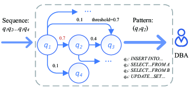
Figure 1. An example of workload pattern discovery.

1. Introduction

Enterprises and consumers are increasingly hosting their services on cloud database systems, e.g., Alibaba Cloud Relational Database Service (RDS) (Alibaba Cloud, 2022), AWS RDS (Amazon EC, 2015), Microsoft Azure SQL Database (Copel et al., 2015), and Google Cloud SQL (Krishnan and Gonzalez, 2015). With the advancement of cloud database technology, these systems can now support a wider range of optimizations, e.g., automatic query re-write (Das et al., 2019), root cause diagnose (Yoon et al., 2016; Ma et al., 2020; Liu et al., 2022), automatic scale-up instances (Liu et al., 2022), and automatic tuning (Duan et al., 2009). The optimization techniques (Das et al., 2019; Yoon et al., 2016; Ma et al., 2020; Liu et al., 2022; Duan et al., 2009) have significantly improved the performance of Database Management System (DBMS), in terms of both the overall system and the specific query execution. Workload pattern discovery can be used to further optimize DBMS performance by providing statistics about entire patterns in the workload, which can significantly enrich the context of existing reports (Tran et al., 2015). An example of workload pattern mining is shown as follows.

Example 0.

Fig. 1 shows an example of workload pattern discovery. Given a sequence of queries $q_{1}q_{2}...q_{1}q_{4}$ executed by a DBMS and a probability threshold $0.7$, only $q_{1}q_{2}$ is returned as its probability of occurrence is no smaller than 0.7. On the other hand, $q_{1}q_{2}q_{3}$ is not returned because its probability of occurrence 0.28 ($=$ 0.7$\times$0.4) is smaller than 0.7.

Example 1.1 shows a frequently executed code sequence $q_{1}q_{2}$. Such information is crucial for database administrators (DBAs) and application developers to optimize quering processing and improve application performance. Note that, the frequency of executed code paths may be unavailable without pattern mining, especially if the components of applications work as black boxes (Tran et al., 2015). Workload pattern mining is thus essential in inferring the business logic and user activities. For example, the DBAs for database-as-a-service (DaaS) offerings (e.g., Oracle Cloud and Alibaba Cloud) require knowledge about the business logic. However, due to permission issue, the DBAs generally do not have access to the source code of the applications. In this case, workload pattern mining can provide DBAs with a useful model for tracing workloads. The model offers the DBAs better insight into the applications running in the database and provides developers of applications with the working flow of the application’s logic (Tran et al., 2015).

However, analyzing workload patterns from large-scale industrial cloud databases is challenging, because the query log often contains queries from multiple business logics rather than a single one. To the best of our knowledge, WI (Tran et al., 2015), the only existing study for workload pattern analysis on databases, cannot distinguish the mixed queries and thus cannot be applied to industrial applications.

Example 0.

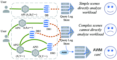
Figure 2. Examples of analyzing workloads from single business logic and multiple business logic.

Fig. 2 depicts two cases of workload pattern discovery. In the upper case, queries (e.g., $A,B,C,\cdots$) from the same business logic (i.e., API) are transferred to a query log store for workload pattern discovery. Since only a single business logic exists in this case, WI (Tran et al., 2015) can be employed without the need for query classification by business logic. In the lower case, queries (e.g., $A,B,C,\cdots$) from multiple business logics (i.e., API1, API2, API3) are mixedly loaded into a query log store. This results in interleaved queries from different business logics in a sequence (e.g., $\{a,X,b\}$, $\{Y,X\}$, and $\{c,Y\}$), which serves as the input of the subsequent workload pattern discovery. This scenario is common in industry applications. WI (Tran et al., 2015), however, cannot distinguish queries from multiple business logics and thus cannot discover workload patterns correctly. The lower case highlights the necessity of distinguishing patterns from multiple business logics in industrial applications.

In this paper, our goal is to develop a system for discovering workload patterns from large-scale query logs and utilizing the discovered patterns to optimize subsequent query processing. Specifically, the system needs to be capable of (i) classifying queries by types of business logic while maintaining users’ privacy, (ii) efficiently performing pattern discovery on each business logic, and (iii) leveraging the discovered patterns to optimize query processing in the cloud database. However, there are four key issues that must be addressed to achieve these objectives.

• Scalability. The system should be designed to handle large-scale datasets, enabling it to train classifiers and identify workload patterns across billions of queries.

• Privacy. A potential classification method is to analyze the App ID and code, which can serve as labels for identifying the business logic. However, such information is considered private and thus is not accessible (Liu et al., 2022) to the system. Therefore, an alternative approach is needed that can classify the data with limited labels.

• Accuracy. Achieving high classification accuracy can be challenging when the true label of a query is mostly unavailable due to user privacy concerns. Thus, it is important to develop classification algorithms that can achieve high accuracy even with limited true labels.

• Optimization. Discovering patterns in query workloads can provide valuable insights into optimizing future query processing in cloud DBMS. However, existing pattern mining systems typically only provide pattern mining results without clear optimization guidelines. This makes it difficult for users who lack knowledge of the underlying logic of database engines to design their own optimization strategies. We thus aim to not only perform pattern discovery but also offer clear optimization guidelines based on discovering results through a user interface.

We present Alibaba Workload Miner (AWM), a comprehensive system that consists of four key modules: Data Collection & Preprocessing Module (DCPM), Offline Training Module (OTM), Online Workload Mining Module (OWMM), and Pattern-based Optimizing Module (POM). The DCPM module is responsible for large-scale data collection and preprocessing. It consists of two feature extraction layers: (i) Workload Semantic Embedding Layer, which utilizes pre-trained foundation models (Kenton and Toutanova, 2019) to extract latent information from SQL queries and provide a rich source of information for classification; and (ii) Execution Feature Process Layer, which encodes execution features, such as response time, into a unified feature that serves as input for the classifier model.

To achieve high scalability, OTM handles heavy workloads efficiently (e.g., label collection and model training), which enables OWMM to infer the trained model and obtain workload patterns in real-time. To preserve privacy, OTM incorporates a novel automatic label method. This method allows users to flexibly select the labels that can be shared as training data. To achieve high accuracy, OWMM employs an effective classifier that categorizes patterns by business logics, with the use of rich features provided by DCPM. Continuing Example 1.2, AWM’ classifier distinguishes $X$ from $a,b$ such that queries from distinct business logic are separated, e.g., $a,b,c,\cdots$ and $X,Y,X,Y\cdots$. This enables effective discovery of workload patterns. To achieve optimization, POM provides users with clear guidelines for optimizing query processing. This allows users to define the business logic-related dependencies for SQL queries by themselves, even if they are not experts in DBMS. In summary, the paper makes the following contributions:

• We develop AWM, an autonomous workload pattern mining system for cloud databases, which discovers frequent workload patterns and provides guidelines for optimizing query processing. To the best of our knowledge, AWM is the first system that has been successfully deployed on large-scale cloud databases.

• We present a high-efficient DCPM. This module can not only process large-scale data in real-time but also extract sufficient latent information from pre-trained foundation models.

• We develop a two-stage framework, OTM and OWMM, for autonomous workload pattern mining. OTM handles complicated tasks with heavy workloads; while OWMM infers the trained model to obtain the discovered patterns promptly in real-time.

• We propose an optimization scheme in POM. It analyzes the discovered patterns by exploiting dependency graphs and provides users with clear guidelines through a user interface. With the guidelines, users can optimize query processing without requiring professional knowledge.

• We conduct extensive experiments on one synthetic dataset and two real-life datasets. The experimental results suggest that compared with the state-of-the-arts, AWM achieves a 70% improvement in the accuracy of pattern discovery and a 25% reduction in the latency of online inference.

The rest of the paper is organized as follows. We present preliminaries in Section 2 and give an overview of the proposed system in Section 3. Section 4 details the DCPM, and Section 5 covers the OWMM. Sections 6 and 7 present OTM and POM, respectively. Section 8 reports the experimental results. Section 9 reviews the related work. Section 10 concludes and offers directions for future work.

2. Preliminaries

2.1. Markov chain

A Markov chain is a type of stochastic model describing a sequence of possible events. A first-order Markov chain considers that the future state depends only on the current state and has nothing to do with the previous state. Put differently, first-order Markov models are memoryless. The $m_{th}$-order Markov chain is an extension of the first-order Markov chain, which considers that the future state depends on the past $n$ states. $m_{th}$-order Markov chains satisfy the following equation of conditional probability:

(1) $$\begin{split}&P\left(X_{t}=x_{t}\mid X_{t-1}=x_{t-1},\ldots,X_{1}=x_{1}\right)\\ &=P\left(X_{t}=x_{t}\mid X_{t-1}=x_{t-1},\ldots,X_{t-m}=x_{t-m}\right)\\ \end{split}$$

where $X_{i}$ and $x_{i}$ represents the $i_{th}$ state of the random variable $X$ and its value, and $t$ is the future state to be identified. The change in the state of a random variable over time steps in a Markov chain is called transition. A transition matrix is generally adopted to describe the structure of a Markov chain. It represents the properties that the Markov chain exhibits during the transition process. A state transition probability is defined as the conditional probability between random variables in a Markov chain.

Markov chains can be exploited to predict and identify the context of SQL queries in the field of workload patterns (Tran et al., 2015). Considering each SQL query as a state of the random variable, Markov chains formulate the transition probabilities among queries in SQL context. Since Markov chains has proven effective for workload pattern mining (Tran et al., 2015), we incorporate Markov chains into AWM.

2.2. Minimum Description Length principle

The Minimum Description Length (MDL) principle (Grünwald, 2007) is a commonly used model selection principle. MDL is particularly suitable for dealing with the selection, prediction, and estimation of complicated models. The quantity of interest (a model or/and parameters) is called a hypothesis. The best hypothesis defined by MDL describes the regularities of data, such that employing it on data compression achieves the highest compression ratio (Li et al., 2020, 2021a). MDL can be formulated according to the maximum a posteriori (MAP) estimation (Grünwald, 2007): $L(D)=\min_{h\in\mathcal{H}}(L(D\mid h)+L(h))$, where $L$ denotes description length. The first term in the formula is the description length of the training data $D$ given the hypothesis $h$. The second term in the formula is the description length of $h$ in the hypothesis space $\mathcal{H}$. The MDL principle selects the hypothesis $h$ that minimizes the sum of these two description lengths. MDL is essentially a balance between model complexity and the number of errors. More specficially, it aims to choose a shorter hypothesis that generates fewer errors.

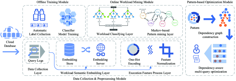
Figure 3. System overview

2.3. Problem Definition

Definition 2.0 (SQL template).

An SQL template (or SQL digest) is a composite of multiple queries that are structurally similar but may have different literal values. An SQL template replaces hard-coded values in the statement with a placeholder (e.g ’?’).

Example 0.

An SQL template "SELECT * FROM item_table WHERE item_id = ?" might include the following children queries:

• SELECT * FROM  item_table  WHERE item_id = ABCDEF

• SELECT * FROM  item_table  WHERE item_id = GHIJKFM

• SELECT * FROM  item_table  WHERE item_id = NOPQRS

Using templates is sufficient for most optimization techniques in practice because the absence of special values has minimal impact on request behavior. A workload pattern is represented by SQL templates, which are interpretable sequences of SQL context in the database’s request behavior. These templates characterize workloads and unveil query patterns that correspond to applications. We formally define it as follows.

Definition 2.0 (workload pattern).

Given a threshold $\alpha$, a workload pattern $p$ is a sequence of queries $q_{1},q_{2},\cdots,q_{m}$, whose occurrence probability is no smaller than $\alpha$.

Definition 2.0 (workload pattern discovery).

Given a query log $Q$ containing a set of queries $q_{1},q_{2},\cdots,q_{n}$, workload pattern discovery aims to find a set of workload patterns $P=\{p_{i}|i=1,2,\cdots,n\}$.

3. System Overview

Table 1. Execution feature collected in the query log store

Feature		Description
lock_wait_time		Waiting time to access data
logical_read		The number of blocks read from memory
rows_examined		The number of rows scanned
rows_returned		The number of rows of data returned
rows_updated		The number of updated data rows
rt		The response time of the transaction
timestamp		The time that the query begins to execute
physical_sync_read		The number of blocks read from disk
database		Name of the database stated in the query
error_code		Execution error code
origin_host		Source database address
sql_type		SQL statement type (e.g., INSERT)
sql		SQL text

We develop a workload pattern discovery system AWM, which actively collects the SQL query patterns logged from the user requests, and then analyzes and provides strategies for optimizing those patterns. We have deployed AWM on Alibaba Cloud Database Autonomous Service (DAS) . The system encompasses four modules: Data Collection & Preprocessing Module (DCPM), Offline Training Module (OTM), Online Workload Mining Module (OWMM), and Pattern-based Optimizing Module (POM). Fig. 3 gives an overview of AWM.

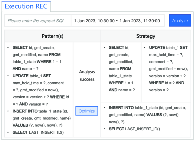
Figure 4. Demonstration of the user interface.

DCPM processes data with three layers: Data Collection Layer, Workload Semantic Embedding Layer and Execution Feature Process Layer. Data Collection Layer collects and pre-processes the streaming raw data (Performance Metrics data and Query Logs data) from millions of database instances in real-time and stores the processed data in a local storage. Workload Semantic Embedding Layer encodes the queries into high-dimensional feature embeddings with rich semantic contexts. Execution Feature Process Layer processes the execution features into uniformed embeddings.

OTM automatically collects training labels and trains classifiers for Workload Classifying Layer with the labels and the pre-processed feature vectors. OWMM discovers workload patterns in a fully online fashion. It has two layers: Workload Classifying Layer and Markov-based Pattern Mining Layer. Workload Classifying Layer encompasses an effective classifier that is trained offline by OTM with few labels. It categorizes query logs by business groups in real-time. Markov-based Pattern Mining Layer receives the classified query logs and performs pattern discovery on them.

POM offers code optimization strategies presented in a user interface to cloud database users. It automatically idnetifies potential optimizations in a set of SQL queries that may arise from sub-optimal business logic code. POM allows users to flexibly define the business logic-related dependencies for SQL queries.

We develop a user interface (UI) that provides a visualization of identified patterns and optimization strategies for users based on their requests. We integrate UI into Alibaba Cloud Database Autonomy Service System, part of which is shown in Fig. 4. In particular, when a user submits a SQL query, AWM analyzes it and displays corresponding patterns and optimization strategies in the UI. Among the strategies shown, SQL queries that appear in the parallel cells of a row can be parallelized.

4. Data Collection & Preprocessing Module

DCPM contains three layers: Data Collection Layer, Workload Semantic Embedding Layer, and Execution Feature Process Layer. When the DBMS executes a SQL query, Data Collection Layer firstly collects all the information related to the query, and then Workload Semantic Embedding Layer encodes the SQL queries into semantic features for a unified process. Meanwhile, Execution Feature Process Layer is applied to obtain the vectorized execution features of the queries. Finally, the two features are fed into both OWMM and OTM as an integrated feature of each query.

4.1. Data Collection Layer

Data Collection Layer collects large-scale streaming query logs data via the Audit log of DB engines (Liu et al., 2022). The query log contains two kinds of information for query execution: the raw query text and the recorded execution data (e.g., query response time). We provide the collected features and the corresponding description in Table 1. Since the data is asynchronously loaded into Alibaba Cloud LogStore (Cao et al., 2021) in real-time, it has little impact on database instances (Mozafari et al., 2013; Theriault and Heney, 1998). Note that, we delete the collected data every three days to avoid storage overflow. We will detail how we encode the input query into a unified feature in Section 4.2 and Section 4.3.

4.2. Workload Semantic Embedding Layer

Input: The input queries $Q$, batch size $b$, pooling method $p$, and the embedding store $D$

Output: Output vector $Z_{o}\in\mathbb{R}^{|Q|\times d}$

1

idx_new $\leftarrow[]$

  // id of queries to be embedded

2 $Q_{n}$ $\leftarrow[]$

3 $Z_{o}\leftarrow 0^{|Q|\times d}$

4 for $i,q\in\textsf{enumerate}(Q)$ do

5      

6      if $q\not\in D$ then

             idx_new.append($i$)

              // add an id to be embedded

7             $Q_{n}$.append($q$)

8            

9      else

             $Z_{o}[i]\leftarrow D[q]$

              // extract value directly from D

10            

11      

12$Z_{n}\leftarrow$FM-Server($Q_{n}$, $b$, $p$)

13 $Z_{o}[\text{idx\_new}]\leftarrow Z_{n}$

14 for $i,q\in enumerate(Q_{n})$ do

15       $D[q]\leftarrow Z_{n}[i]$

16      

17return $Z_{o}$

Algorithm 1 Workload Semantic Embedding Layer

Workload Semantic Embedding Layer pre-processes data by providing sufficient features from the SQL text corpus in a unified vector. This enables Workload Classifying Layer to achieve higher performance with limited training labels.

4.2.1. Deploying the Embedding Server of Foundation Models

Workload Semantic Embedding Layer serves an API online with GPU acceleration to map the SQL query text into a high dimensional embedding space, namely FM-Server. Here, we use the pre-trained foundation models (FMs) (Kenton and Toutanova, 2019; Liu et al., 2019, 2021) to embed the SQL text. This is because FMs can learn latent information from the web, which enhances the classification with fewer training labels. The pre-trained FMs have proven effective for subsequent tasks such as knowledge graphs (Ge et al., 2022) and data integration (Ge et al., 2021b). Since SQL query text is generally text data generated with meaningful statements, incorporating FMs can result in better accuracy (Tang et al., 2022). To implement pre-trained FMs, we adopt the transformers library from hugging face for obtaining an accurate and reliable service. Here, the FM maps an input sequence of SQL text token representations $(x_{1},...,x_{n})$ to a sequence of continuous representations $\mathbf{z}=(z_{1},...,z_{n})$, where $x$ is a token, $(x_{1},...,x_{n})$ is the whole query text, and $z_{i}\in\mathbb{R}^{d}$ is the vector representation of dimension $d$ indicating the embedding of $x_{i}$. An example is shown as follows.

Example 0.

Given an SQL query text "SELECT id, name FROM user_table WHERE id=5", and a simple tokenizer dividing the text by space, we get a list of tokens $T=$ ["SELECT", "id,", "name", "FROM", "user_table", "WHERE", "id=5"]. For this SQL text, the FM outputs a vector $Z\in\mathbb{R}^{|T|\times d}$ where $|T|$ indicates the length of the token list.

In practice, more complex tokenizers (Kenton and Toutanova, 2019) are employed in the upstream tasks of pre-trained FMs. Here, we process the queries by batch to speed up the overall procedure. Thus, with a batch of query texts, a vector $Z_{b}\in\mathbb{R}^{b\times max(|T|)\times d}$ is obtained, where $b$ is the batch size. Note that, the middle dimension of $Z_{b}$ is $max(|T|)$, which indicates the FM pads the output in order to align the output length of all sequences. Suppose we have a batch, in which the shortest sequence length is $t$, then the output of this sequence will be a vector of $max(|T|)\times d$. In this vector, only the prefix of $t\times d$ has the valid semantic value, and the rest is padded with a constant number zero by default.

After applying FM, we map the sequence of vectors $Z_{b}$ for each SQL statement into a unified size vector $Z_{o}\in\mathbb{R}^{b\times d}$, to be prepared for the downstream tasks. This incurs the demand for pooling, which reduces the sequence of vectors into one vector. We support two types of pooling methods: (1) max pooling, which returns the maximum value along the given dimension; and (2) mean pooling, which returns the averaged value along the given dimension. In each pooling method, we pool the result matrix along the sequence dimension. Thus, for each value of the output vector, the result is reduced from all the tokens acquired by FM, i.e., the original $Z_{b}\in\mathbb{R}^{b\times max(|T|)\times d}$ is transformed into $Z_{o}\in\mathbb{R}^{b\times d}$ by pooling.

Since the output is a padded vector, the padded value will have an adverse effect on the result. By using the default constant, we discuss the following two cases: (i) when using max pooling, we may be unable to get a negative value from the FM; and (ii) when using mean pooling, we may obtain a relatively smaller output vector in terms of the norm. To avoid these, we first augment the output (e.g., for max pooling, we pad the output vectors with $-\infty$), and then calculate the mean or max value.

Input: The input queries $Q$, batch size $b$, pooling method $p$

Output: Output vector $Z$

1

2

3def FM-Server($Q$, $b$, $p$):

4      

5      $\textit{batch\_idx}\leftarrow$ 0

6      

7      result $\leftarrow[]$

8      while $\textit{batch\_idx}<|Q|$ do

9             $\textit{batch\_end}=min(\textit{batch\_idx}+b,|Q|)$

10             $query\_batch=Q[\textit{batch\_idx}:\textit{batch\_end}]$

11             $T_{b}\leftarrow$ Tokenizer($query\_batch$)

12             $S_{T}\leftarrow len(T\;\text{for}\;T\;\text{in}T_{b})$

13             $Z_{b}\leftarrow$Pooling_Mask( Language_Model($T_{b}$), $S_{T}$, $p$)

14            

15            if $p$ is "max_pooling" then

16                  

17                  $Z\leftarrow Z_{b}.\text{max(axis=1,keepdim=False)}$

18                  

19            if $p$ is "mean_pooling" then

20                  

21                  $Z\leftarrow Z_{b}.\text{mean(axis=1,keepdim=False)}$

22                  

23            

24            $\textit{batch\_idx}\leftarrow\textit{batch\_idx}+b$

25             $\textit{result}\text{.append(}Z\text{)}$

26            

27      return concatent(result)

Algorithm 2 FM-Server

4.2.2. Embedding Store

We observe that most of the SQL queries executed are repeated. Thus, we develop an embedding store to cache the output feature embeddings. The embedding store should satisfy the following two requirements. First, it should follow idempotence (Richardson and Ruby, 2008) of Workload Semantic Embedding Layer. This means that, for one specific input, Workload Semantic Embedding Layer can be applied several times, but the resulting state of one call should be indistinguishable from the consequent state of multiple calls. This results in a consistent handling function of duplicate requests received by the API. Duplicate requests may arrive unintentionally or intentionally. For example, a user may send several duplicate queries due to timeout or network issues. However, the output embeddings of FMs may be different in terms of the batch context, which is not desirable. Second, FM-Server requires massive computational resources. Thus, applying it to infer massive queries in real-time is unrealistic and inefficient (cf. Section 8).

To address the above-mentioned issue, we hash the SQL text of each input and store its unique embedding index by a global hash map. For each newly emerged query, we first check if the query text has been computed. If it has, we directly output the stored embedding; if it has not, we compute the feature embedding with FM-Server, and then store it in the embedding store.

The pseudo-code of Workload Semantic Embedding Layer is shown in Algorithm. 1. Given the input $Q$, which is the set of SQL query texts, the algorithm first initializes the output memory space and other supporting variables (cf. Lines 1-3 of Algorithm 1). Then, for each query, we check if its embedding has already been calculated. If it has, the value is directly obtained  (cf. Lines 4-9 of Algorithm 1). The embedding queries that are not cached by the embedding store are then calculated online and merged into all features  (cf. Lines 10-11 of Algorithm 1). Next, we update the embedding store and return the currently requested vectors.

The implementation of FM-Server is shown in Algorithm 2, which follows a batched design to infer the foundation model. For each batch, we first compute the tokens and other supplementary features  (cf. Lines 4-8 of Algorithm 2). Then, we apply FM to the queries and assign corresponding values to padded positions for different pooling methods. To pad the right value for reduction, we calculate a mask for each query token sequence, indicating the position of the padded value. If the pooling method is "max pooling", a very small number ($-\infty$) is padded. For "mean pooling", we first pad the value to 0 and then scale the whole batch  (cf. Lines 9-13 of Algorithm 2). Finally, we reduce the output size by pooling the embedding and proceed to the next batch  (cf. Lines 10-15 of Algorithm 2).

4.3. Execution Feature Process Layer

The classification model generally can only take numerical value as the input to make the regression prediction. In this section, we detail how we use Execution Feature Process Layer to preprocess the recorded execution data into numerical data, in order to sufficiently learn all feature information of each query.

The data features and the corresponding description are shown in Table 1. We divide all features into two primary categories: (i) features with numerical meaning (e.g., rows_examined, logical_read, and rt) and (ii) features without numerical meaning (e.g., origin_host, error_code, and sql_type). For the first category, we normalize them with their mean value and std. For the latter category, OneHot is adopted to encode their input variables. As a common encoding method in machine learning, OneHot encoding uses N-bit 0/1 registers to encode N states.

Note that, when numerical features follow long tail distribution, directly encoding them tends to result in high data dimension. Hence, we preprocess numerical features before label encoding or OneHot encoding to modify its representation. For example, the rows_examined feature is represented as ten integer values from $1$ to $10$ based on its numerical distribution. In addition, some features have special significance when their values are zero (e.g. the query is most likely a SELECT statement when its rows_updated is 0), and we represent such features as specified integers.

5. Online Workload Mining Module

OWMM acts as a real-time service. It contains two layers: Workload Classifying Layer and Markov-based Pattern Mining Layer. When a query arrives, Workload Classifying Layer first receives the features of this query from DCPM for classification by business groups. Then, Markov-based Pattern Mining Layer of the corresponding business group processes this query.

5.1. Workload Classifying Layer

In this layer, we classify the queries into different business groups. The input of each query contains: the semantic embedding $Z$ based on Workload Semantic Embedding Layer and the query execution information $X$ based on Execution Feature Process Layer. More specifically, we first concatenate the two features to obtain a unified input vector of each query, i.e., $F=[Z||X]$. Then, we can apply a classification model to the input embeddings, i.e., $clf(F)$, where $clf$ is the pre-trained classifier. Although Workload Classifying Layer can incorporate any kind of classifier model, it cannot be specified by users because it is a general classifier for all users and is thus hard to satisfy users’ localized and specialized needs. This paper sets XGBoost Classifier (XGBClassifier) (Chen and Guestrin, 2016) as the default classification model due to its high scalability.

5.2. Markov-based Pattern Mining Layer

This layer is to discover workload patterns from SQL queries filtered by Workload Classifying Layer, where the Markov chain model and Oracle Workload Intelligence (WI) (Tran et al., 2015) model are employed. In the following, we introduce this layer by detailing the transformation from SQL query texts to templates, the Markov model selection and the workload patterns mining.

5.2.1. Transform SQL query texts into Templates

To handle massive SQL queries, we transform SQL query texts into SQL templates according to the equivalence of the operation. Specifically, we first gain SQL templates (MySQL 8.0 Reference Manual, 2022; Tran et al., 2015; Ma et al., 2018; Verbitski et al., 2017) based on its definition (cf. Section 2.3). Next, we hash the template via a unique SQL_ID. Finally, we identify a set of SQL queries as equivalent among the discovered patterns if their SQL_IDs are identical.

5.2.2. Select the appropriate Markov model

We build a prefix tree for the SQL sequence $S$ for analyzing and calculating the state transition probabilities using MDL principle (Tran et al., 2015). The prefix tree is an ordered tree with $max\_ord+2$ layers of nodes, where $max\_ord$ is the maximum order of the Markov model. The root node is at the first level, i.e., level zero, and the leaf nodes are at the last level, i.e., level $max\_ord+1$. Each node in the prefix tree represents an ordered sequence. The edge between nodes represents a statement, and the node stores the occurrence frequency of its represented ordered sequence.

Example 0.

Given a SQL sequence $S=q_{1}q_{2}q_{3}q_{4}q_{3}q_{4}q_{2}q_{3}q_{4}q_{3}q_{1}q_{3}\\ q_{4}q_{3}q_{2}q_{5}$ and the maximum order of Markov model ${max\_{ord}}=1$, a prefix tree is constructed, as shown in Fig. 5. To be specific, $n_{2}=3$ represents that $q_{2}$ appears 3 times in the sequence; $n_{8}=2$ represents that $q_{2}q_{3}$ appears 2 times in the sequence.

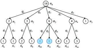
Figure 5. A prefix tree for Example 5.1.

In order to reduce the time cost and improve the generalization ability of the model, we prune the built prefix tree to calculate state transition probabilities before applying MDL principle. Specifically, the state transition probabilities are computed by $\mathrm{P}\left(q_{x}\mid\mathrm{s}\right)=\frac{\operatorname{value}\left(n_{c}\right)}{\operatorname{value}\left(n_{p}\right)}$, where $s$ and $n_{p}$ represent the current sequence and its corresponding node, while $q_{x}$ and $n_{c}$ represent the new query and its corresponding node. However, when calculating the nodes in the same layer, the probability may be 0, which ignores the appearance possibility of some sequences and affects the subsequent model selection. Hence, it is necessary to modify the method of computing state transition probabilities according to the threshold $\tau=1/|\operatorname{set}(S)|$:

• If $\mathrm{P}\left(q_{x}\mid\mathrm{s}\right)\geq\tau$, the transition probability follows its corresponding real distribution;

• If $\mathrm{P}\left(q_{x}\mid\mathrm{s}\right)<\tau$, the transition probability is considered to be distributed uniformly.

Example 0.

Continuing Example 5.1 and given $\tau=1/|\operatorname{set}(S)|=1/5$, $P\left(q_{4}\mid q_{3}\right)=\frac{\operatorname{value}\left(n_{12}\right)}{\operatorname{value}\left(n_{3}\right)}=\frac{2}{3}>\frac{1}{5}$. Thus, $P\left(q_{4}\mid q_{3}\right)$ is preserved as its real distribution. On the contrary, due to $P\left(q_{2}\mid q_{3}\right)=P\left(q_{1}\mid q_{3}\right)=\frac{\operatorname{value}\left(n_{10}\right)}{\text{ value }\left(n_{3}\right)}=\frac{1}{6}<\frac{1}{5}$ and $P\left(q_{3}\mid q_{3}\right)=P\left(q_{5}\mid q_{3}\right)=0<\frac{1}{5}$ $P\left(q_{2}\mid q_{3}\right)$, $P\left(q_{1}\mid q_{3}\right)$, $P\left(q_{3}\mid q_{3}\right)$ , and $P\left(q_{5}\mid q_{3}\right)$ are all set to $\left(1-P\left(q_{4}\mid q_{3}\right)\right)/4=\frac{1}{12}$.

In order to choose the most suitable Markov model, we calculate the costs of pruned models with different orders according to MDL principle following (Tran et al., 2015):

(2) $$\begin{split}\mathbb{C}\left(S,M^{{ord}}\right)=2\times(\log{ord}+\log m+1)\\ +m(({ord}+1)\log|\operatorname{set}(S)|+2\log|S|)\\ -\log\mathrm{P}\left(S\mid M^{{ord}}\right)\end{split}$$

where $M^{ord}$ is the Markov model of ${ord}_{th}$ order; $m$ is the number of items whose probability values reach the threshold $\tau$; $\operatorname{set}(S)$ is the statement set of SQL sequence $S$; and $\mathrm{P}\left(S\mid M^{{ord}}\right)$ is the probability calculated by continuous multiplication. Continuing Example 5.2 where order of Markov model is 1, $\mathrm{P}\left(S\mid M^{{ord}}\right)$ is derived as follows.

(3) $$\begin{split}\mathrm{P}\left(S\mid M^{{ord}}\right)=P\left(q_{1}\right)\times P\left(q_{2}\mid q_{1}\right)\times P\left(q_{3}\mid q_{2}\right)\times P\left(q_{4}\mid q_{3}\right)\\ \times P\left(q_{3}\mid q_{4}\right)\times\cdots\times P\left(q_{5}\mid q_{2}\right)\end{split}$$

Finally, the $x_{th}$ order Markov model with the smallest cost is selected. We calculate the required state transition matrix from the Markov model with the order selected.

5.2.3. Discover workload patterns

After obtaining the state transition matrix and the Markov model order $x$, we proceed to determine whether an SQL sequence is a pattern by following WI (Tran et al., 2015). Specifically, given a threshold $\theta$, $q_{1}\ldots q_{x}q_{y}$ is identified as a pattern if the state transition probability $\mathrm{P}\left(q_{y}\mid q_{1}\ldots q_{x}\right)\geq\theta$.

Example 0.

Continuing Example 5.1, we set the threshold $\theta$ to $0.7$ and the Markov model order to $1$. We first initialize the pattern as $q_{1}$. Since $P\left(q_{2}\mid q_{1}\right)=\frac{1}{2}<\theta$, $q_{1}$ is returned as pattern. Next, we reset the new pattern as $q_{2}$ and continue the calculation until the new pattern is reset to $q_{4}$, where $P\left(q_{3}\mid q_{4}\right)=\frac{3}{4}>\theta$. As a consequence, we update the pattern as $q_{4}q_{3}$. Since $P\left(q_{4}\mid q_{3}\right)=\frac{2}{3}<\theta$, $q_{4}q_{3}$ is returned as a pattern. We repeat this procedure until reaching the end of the sequence.

6. Offline Training Module

In this section, we detail the implementation of OTM, which is employed to train parameters offline.

6.1. Automatic Label Collection

As discussed in Section 5, it is necessary to classify the queries stored in SQL query log into different business groups. To achieve this, we need to collect labels to train a classifier. We divide label collection into two parts: label collection for public data, and label collection for industrial data. Note that, in order to avoid the heavy back prop operations caused by the update of the foundation model, we do not fine-tune FMs.

6.1.1. Label collection for public data

It is uncommon for public datasets to log different businesses into one query log. This is because the currently available datasets are obtained from relatively simple business logic, and do not meet the requirement of large-scale complex business. To this end, we propose a generated dataset by fusing multiple public datasets (cf. Section 8), whose ground truth label is obviously available.

6.1.2. Label collection for industrial data

We aim to protect user privacy when collecting labeled SQL queries from industry applications. This implies that we should minimize the labels we collect without compromising classification accuracy.

We provide users with a unique ID for each business group. Requests with the unique ID may pass through another API that is encapsulated by the cloud database interface, which is generally non-transparent to users. This implies that users only need to pass this unique ID as an extra data field when logging in to the cloud database. With the unique ID, we provide three options for users to label their business groups.

Random Sample. When the user queries the cloud database, the system will send the query with a probability $P_{L}$, where $P_{L}$ is a configurable parameter. The default value of $P_{L}$ is $0.01$, indicating that 1% of the total requests are marked as training labels to classify the business groups.

Manually Labeling. Users can flexibly choose the queries to be labeled, by informing the system of their preferences. This preserves the user privacy.

Hybrid. When employing random sampling, users are allowed to manually specify the type of SQL query that is prohibited from accessing as the training label. Specifically, this is achieved by setting a flag when querying the SQL statement. The flag overwrites the global probability $P_{L}$ so that the queries with the flag will not be sampled by the system. This setting aims to balance the label quality and user privacy.

When Random Sample and Hybrid are adopted, the classifier model is trained on a weekly basis by default and the frequency of updating the model is configurable. After training, the labeled SQL queries are discarded to prevent possible data/privacy leakage. When Manually Labeling is adopted, the classifier model is trained only when the user requests the model to be updated.

6.2. Classifier Model Training

The parameters involved in Workload Classifying Layer should be trained accurately, which is a prerequisite for having Workload Classifying Layer perform classification efficiently. To achieve this, we need to carefully select the training data. It can be collected from business groups who have executed massive SQL queries on the cloud database server. Note that, in order to protect user privacy, we aim to minimize the number of labels we collect. We adopt XGBClassifier (Chen and Guestrin, 2016) as the classifier model. However, AWM also accommodates other classifier models (cf. Section 8).

As the size of the input data is extremely large, the model training follows a mini-batch strategy. Specifically, we separate the data by the ‘timestamp’ feature and train the model in small batches.

7. Pattern-based Optimizing Module

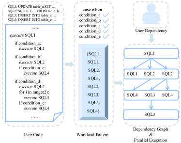
Figure 6. An example of optimizing query code.

As an application of AWM, POM analyzes the workload patterns discovered by OWMM and provides optimization strategies for cloud database users to improve their business logic codes. Optimizing queries based on mined workload patterns can fundamentally optimize the business, which is more valuable than optimizing based on the entire workload extracted from logs directly.

In general, the workload patterns from one business group typically have two origins. The first is the pattern within one piece of code. For example, a function that first executes the "SELECT" command on the "user" table to select requested user IDs, and then iteratively "SELECT" and "UPDATE" the followers of the user. This creates a pattern of "SELECT uid" $\rightarrow$ "SELECT follower" $\rightarrow$ "UPDATE follower" $\rightarrow$… . The second is the pattern generated from the business group, which is the remote procedure call (RPC) from different micro-services. The reason is that the modern implementation of business logic follows the micro-service architecture (Nadareishvili et al., 2016), which enables back-end programmers to reduce code coupling. This strategy is adopted by most large tech companies. This motivates us to take advantage of the analysis of this strategy. Specifically, in POM, micro-services call each other to form a directed acyclic graph (DAG) with a call relationship in a user’s request.

In both of the above situations, dependencies exist within the codes querying the cloud database, either intentional or not intentional. Furthermore, the dependencies are hidden inside the patterns discovered from the SQL query log corpus. For SQL queries without dependencies in-between each other, executing them in parallel is obviously more efficient. Since a pattern is a sequence of queries that occurs frequently, optimizing the execution of patterns is more significant than that of infrequently occurred queries. Hence, our goal is to analyze the workload patterns and figure out strategies for users to execute SQL queries in parallel (as shown in Fig. 6). To achieve this, we represent the dependencies as a graph and propose Dependency aware Multi-query Optimizer for constructing the dependency graph within queries. Based on this, we provide optimization based on the constructed graph.

⬇

// business-based dependency

if ("SELECT count(*) FROM users"==10){

items = "SELECT … FROM items"

shops = "SELECT … FROM shops"

// block-based dependency

"UPDATE users SET … WHERE …"

…

}

Figure 7. An example of query code.

7.1. Dependency aware Multi-query Optimizer

7.1.1. Dependency graph construction

Two types of dependencies are related to constructing the dependency graph. The first type (namely block-based dependencies) is the dependencies that are trivially inferred from the SQL query text. For example, if there is one "SELECT" operation after an "UPDATE" operation, and the two queries are applied to the same table, then the "SELECT" should not be executed until the "UPDATE" is completed. Intuitively, this type of dependency can be directly derived from the data. The second type of dependency (namely business-based dependencies) is the business logic-related dependency and is not accessible for the cloud database. Example 7.1 gives an example.

Example 0.

Assume that the user has written some codes starting with an "if" statement, which is to check whether a "SELECT" statement returns any possible value (as shown in Fig. 7). If it does, the program will run two "SELECT"s to check further requirements, and then run an "UPDATE" to update the table.

Example 7.1 suggests that the first "SELECT" blocks the followed-up operations. However, it cannot be detected by the cloud database, as it is not a blocking query. Since it is hard to detect this type of dependency by using only the limited knowledge stored in the cloud database, we provide the users an interface, by which they can input such dependency and we can then collect it.

Next, we introduce the generation of dependency graph from query patterns. Considering the block-based dependencies, it is essential to detect the blocking queries. Such queries may block followed-up queries to execute, e.g., an "UPDATE" query is a blocking query. Different blocking queries have different scopes of blocking. For example, the DDL (Data Definition Language, e.g., "CREATE", "ALTER") queries generally have larger scopes than the DML (Data Manipulation Language, e.g., "INSERT", "UPDATE") queries. To construct the graph, we iterate the pattern. For each scope (database/table), we maintain a map of the current blocking query. If the query is within a scope (e.g., is querying a specified table), we add one dependency edge between the blocking query of this scope and the current query. If the query itself is a blocking query, we update the corresponding scope in the map. For those business-based dependencies, we provide interfaces for users to define their specified dependencies.

7.1.2. Dependency-graph-based optimization

After the dependency graph $G$ is built, Dependency aware Multi-query Optimizer performs a breadth-first search on $G$ to determine the optimal execution order of queries. Once the optimization result is generated, users receive a list of queries that can be executed in parallel in the same order. In the case of incorrect results, users can manually add dependencies and the system will update the order accordingly. By following the suggestions provided by the system, users can further optimize their code for improved performance.

Table 2. Comparison results.

		AQL-N					AQL-L					OSQL
Setting	Method	Pattern Precision	#	F1	Latency	Time	Pattern Precision	#	F1	Latency	Time	Pattern Precision	#	F1	Latency	Time
-	WI	0%	0	-	0.00302	-	0%	0	-	0.00335	-	3.92%	2	-	0.35479	-
-	WI-tid	15.24%	25	-	0.00254	-	0.79%	25	-	0.00487	-	-	-	-	-	-
-	WI-kmeans	25.37%	17	-	-	2007.80	17.39%	20	-	-	9899.11	20.00%	16	-	-	285.41
E		86.54%	45	99.21%	0.00246	169.45	83.78%	62	99.13%	0.00253	769.23	81.72%	76	91.71%	0.27956	7.50
L		88.00%	44	99.39%	0.00246	290.08	84.00%	63	99.55%	0.00258	1,904.86	90.63%	87	93.98%	0.26061	16.05
N	AWM	89.58%	43	99.45%	0.00247	402.44	86.49%	64	99.60%	0.00260	2,643.84	90.91%	90	94.10%	0.25213	28.07

• ^∗F1 is to measure the performance of Workload Classifying Layer and Precision is to measure the overall pattern discovery performance.

8. Experimental Evaluation

We report on extensive experiments aimed at evaluating the performance of AWM.

8.1. Experimental Setup

Experimental dataset. We use two real-life datasets (AQL-N and AQL-L) and one synthetic dataset (OSQL).

• AQL-N. It is a normal query log of the Alibaba Cloud database. It contains 941K queries, of which the number of SQL templates is 184. The total query response time of AQL-N is 683.22 seconds.

• AQL-L. It is a large query log of the Alibaba Cloud database. It contains 4.5M queries, of which the number of SQL templates is 205. The total query response time of AQL-L is 2,512.59 seconds.

• OSQL. AWM is designed to discover workload patterns from multiple sources. However, no public integrated dataset is available, Thus, we synthesize a dataset by fusing four public datasets: StackOverflow (Iyer et al., 2016), IIT Bombay (Chandra et al., 2015), UB dataset (Kul et al., 2018), and PocketData (Kennedy et al., 2015). Specifically, we randomly sample queries from the four datasets and then mix them into OSQL. OSQL contains 4,403 queries, of which the number of SQL templates is 4,308. Since the four public datasets (StackOverflow, IIT Bombay, UB dataset, and PocketData) only provide the query statement texts but not the query execution feature, the total query response time of OSQL is unknown.

AQL-N and AQL-L from Alibaba Cloud are diversified and complicated. Diversified means that they contain not only a large number of entries but also a variety of information such as SQL text and execution feature metrics. Complicated means that they contain query entries from different business logic and database instances. We collect the SQL data from a certain application of the Alibaba Cloud database as the ground truth, in order to test the performance of AWM on AQL-N and AQL-L. On the other hand, OSQL only contains a small number of queries with the repetition rates of templates being low. This implies that most patterns of OSQL have shorter lengths. Since no ground truth is available, we collect data from each source of OSQL and apply Markov-based Pattern Mining Layer to generate ground truth patterns.

Evaluation metrics. We study the performance of AWM in terms of Effectiveness of pattern mining, Effectiveness of Workload Classifying Layer, and Efficiency of AWM. Effectiveness of pattern mining is measured by the number of correctly discovered patterns (# of pattern) and precision (Precision). Effectiveness of Workload Classifying Layer is measured by F1-Score(F1). Efficiency of AWM is measured by logging the online serving latency of OWMM (Latency) and the offline training time of OTM (Time).

Baselines. We compare AWM with three baselines: WI (Tran et al., 2015), WI-tid, and WI-kmeans. WI mines the patterns of SQL context based on a Markov chain-based method, which is the state-of-the-art work for workload pattern discovery. However, WI is designed for mining patters with a single business logic, and thus cannot be directly applied to discovery patterns in cloud databases (cf. Section 1).

To attain a fair comparison, we provide two variants of WI: WI-tid and WI-kmeans, both of which adapt WI to cloud databases. WI-tid classifies the queries of AQL-N and AQL-L using the tid (i.e., the thread id of the program to access the database) attribute of the data source. This way, queries from multiple sources can be distinguished according to the characteristic of the business logic. After classification, WI-tid exploits WI to discover patterns for each category respectively. WI-kmeans performs classification in an unsupervised way, where the data is automatically categorized. Specifically, WI-kmeans first adopts K-Means to cluster data, and then discovers patterns for each cluster with WI.

Implementation details. We set the maximum order of the Markov model to 1 and $\theta$ to 0.77 for all baselines. When implementing WI-kmeans, we set the number of clusters to 5 for AQL-N and AQL-L, and 15 for OSQL. We use the encoded query features obtained from Execution Feature Process Layer to cluster the queries for AQL-N and AQL-L. Since the query execution feature is unavailable, we apply Workload Semantic Embedding Layer to the query texts and take the embeddings as the clustering input. All the baselines do not have a classification model. Thus, we do not report F1 and Time for them. Since WI-kmeans runs clustering on the whole dataset, it is infeasible to apply it to online scenarios. Hence, we do not report the Latency for WI-kmeans. Moreover, Time of WI-kmeans refers to the end-to-end workload discovery time. We set three training set ratios (proportion of the data used for training) for each dataset, respectively, when studying the performance of AWM. The lowest training set ratio is denoted as E; the highest training set ratio is denoted as N; and the middle training set ratio is denoted as L. For AQL-N and AQL-L, we choose 1% (E), 5% (L), and 10% (N) of the total data of AQL-N, AQL-L, and OSQL as training sets, respectively. Here, the highest training ratio (10%) is below the commonly used settings of existing classification tasks (Chen and Guestrin, 2016); while the lowest training ratio (1%) is extremely smaller than the one adopted by most of the classification tasks (Chen and Guestrin, 2016). For OSQL, we choose 20% (E), 40% (L), 60% (N) of the total data of AQL-N, AQL-L, and OSQL as training sets, respectively. Here, we use a larger proportion of training data because the query execution features of OSQL are unavailable. We employ the max pooling method and a batch size of 512 for the Workload Semantic Embedding Layer’s foundation model. We select multi:softmax as the loss function and mlogloss as the evaluation function for Workload Classifying Layer. We use the same setting as WI when implementing Markov-based Pattern Mining Layer. We set the number of batches to 10 for Execution Feature Process Layer of AQL-L.

8.2. Comparison Study

We compare AWM with WI (Tran et al., 2015), WI-tid and WI-kmeans in terms of effectiveness and efficiency. AWM, WI and WI-kmeans are performed on AQL-N, AQL-L, and OSQL, while WI-tid is performed only on AQL-N and AQL-L. This is because WI-tid conducts classification by exploiting the tid attribute (cf. Section  8.1), which is missed in OSQL. Table 2 shows the comparison results.

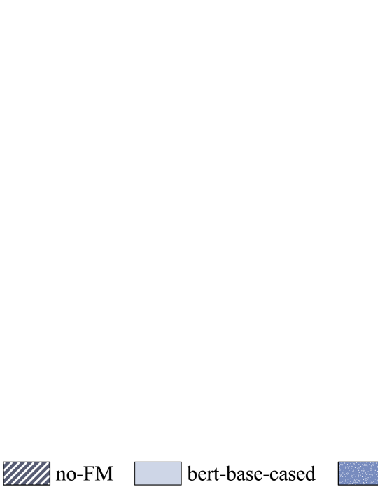
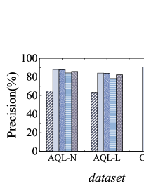
(a) Pattern Precision

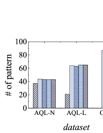
(b) # of pattern

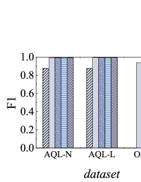
(c) F1

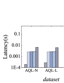
(d) Latency

Figure 8. The results of varying foundation models.

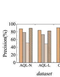
(a) Pattern Precision

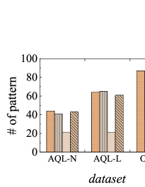
(b) # of pattern

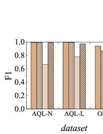
(c) F1

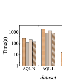
(d) Time

Figure 9. The results of varying classifiers.

8.2.1. Effectiveness Study.

As observed in Table 2, AWM outperforms three baselines significantly in terms of Pattern Precision and # of pattern on all datasets. First, Pattern Precision of AWM is more than 81% and F1 is more than 91% on all datasets. Specifically, AWM improves Pattern Precision by more than 60% compared to WI-kmeans, which achieves the highest Pattern Precision among all baselines. Next, patterns identified by AWM (# of the pattern) are 18 and 37 more than WI-tid on AQL-N and AQL-L, respectively, and are 60 more than WI-kmeans on OSQL. These results highlight the effectiveness of AWM. This is attributed to the use of XGBClassifier (Chen and Guestrin, 2016; Ma et al., 2020; Yoon et al., 2016) model in OTM, which takes into account data characteristics to more accurately mine patterns. Note that, both Pattern Precision and # of the pattern of WI on AQL-N and AQL-L is 0. This is because WI is designed for a single database and small-scale data only (cf. Section  8.1) and struggles when processing large-scale industrial data.

Third, the increase of training data leads to growths of F1, Pattern Precision and # of pattern, because more training labels lead to higher accuracy of training. However, even with the minimum training set ratios, AWM is able to outperform all baselines significantly. The reason is that Automatic Label Collection enables AWM to work with limited resources, where the user privacy is protected by Automatic Label Collection (cf. Section 6.1).

8.2.2. Efficiency Study

As shown in Table 2, AWM’s Latency is significantly lower than the three baselines’ on three datasets. Specifically, AWM reduces Latency by 2.7% compared with WI-tid on AQL-N and reduces Latency by 22% and 21% compared with WI on AQL-L and OSQL, respectively. Here, WI-tid achieves the lowest Latency among all baselines on AQL-N and WI achieves the lowest Latency among all baselines on AQL-L and OSQL, respectively. The above mentioned experimental results are mainly because (i) when processing large-scale data, all baselines generate large Markov models, resulting in a large time overhead; (ii) WI-kmeans performs clustering offline; and (iii) AWM reduces the sizes of Markov models by discovering patterns for each category respectively and separating offline training from online classification and workload pattern discovery.

Next, Latency of all methods on OSQL is significantly higher than those of the other two datasets. This is because Latency largely depends on the number of SQL templates. As mentioned in Section  8.1, OSQL has more SQL templates and a lower repetition rate of SQL queries than AQL-L and AQL-N. This leads to higher time and space costs for selecting an appropriate Markov model in Markov-based Pattern Mining Layer. Meanwhile, the latency of WI-tid on AQL-L is higher than that on AQL-N. This reason is that when processing massive data, classifying by tid tends to generate more repeated patterns, which increases the time cost.

Although it is true that AWM requires additional time for training the classification model offline, its time cost is still acceptable for processing millions of data. As the size of data used for training the classification model grows, the Time of AWM increases. However, AWM requires only 100 seconds to train the model, which is negligible compared to the total query time (about 1 hour). Note that, Time of WI-kmeans is much larger than AWM because it mines all workload patterns in an offline fashion.

8.3. Ablation Study

8.3.1. Analysis of foundation models

Fig. 8 reports the effects of four foundation models, bert-base-cased (Kenton and Toutanova, 2019), roberta-base (Liu et al., 2019), xlm-roberta-base (Conneau et al., 2020) and xlm-roberta-large (Conneau et al., 2020) by applying them to AWM respectively. We set the training ratio of each dataset to the corresponding lowest one, i.e., 1% on AQL-L and AQL-N, and 20% on OSQL (cf. Section 8.1). no-FM denotes the case where we do not use any foundation model. Note that, no-FM has not been studied on OSQL because SQL text is the only available information for the public datasets (Iyer et al., 2016; Chandra et al., 2015; Kul et al., 2018; Kennedy et al., 2015) (cf. Section 8.1).

The results suggest that using foundation models in AWM can improve its performance in terms of F1, Pattern Precision and # of pattern. Although the use of foundation models does incur some time cost, the improvement in performance is significant and acceptable (cf. Section 4.2.2 and Section 8.4). Next, the bert-base-cased model achieves the best performance on each dataset, indicating that it is more universal than other models. The xlm-roberta-base model performs the worst in OSQL while performing well on the other two datasets. This is because the training data of xlm-roberta-base model differs largely from OSQL. Meanwhile, we observe that when processing large-scale data, a small deviation in-between F1 may indicate a huge gap in between the number of correctly discovered patterns. Finally, xlm-roberta-large model’s Latency is 2 times larger than other foundation models’. The reason is that the size of xlm-roberta-large model is the largest among the three models, and thus results in the largest embedding dimension and longest time for preprocessing in DCPM.

8.3.2. Analysis of classifier.

Fig. 9 shows the effect of using different classifiers. As observed, XGBClassifier and MLPClassifier are more suitable for AQL-N and AQL-L, while SVC is more suitable for OSQL. This is because OSQL have more SQL templates. On the other hand, AQL-N and AQL-L only have around 200 unique templates and contain additional execution features which do not fit the SVC model. Moreover, according to the experimental results on AQL-L, Time grows with the data size, because we employ batch processing to trade time for space.

8.4. Scalability Study

We study the scalability of the Embedding store and OTM of AWM on AQL-N and AQL-L. We remove the Embedding store (by applying FMs online to obtain the embedding) and OTM from AWM, respectively. We denote the system without the Embedding store as AWM-Embedding store and the system without OTM as AWM-OTM. Then we compare them with AWM, respectively. Note that, since directly calculating the embeddings of the whole dataset is infeasible, we randomly sample 2% data of the total data and record Latency of AWM, AWM-Embedding store, and AWM-OTM on it.

The experimental results are reported in Fig. 10. First, as shown in Fig. 10a, Latency of AWM-Embedding store is 10 times higher than that of AWM. This verifies that employing the Embedding store can greatly reduce the time for computing the embedding of massive data, thereby improving the efficiency of AWM. Next, as shown in Fig. 10b, Latency of AWM-OTM is 1.15 times higher than that of AWM. This is because AWM trains data offline, which is more efficient.

8.5. Study of Pattern-based Optimizing Module

We evaluate the effectiveness of POM. We collect ten user cases in an internal software evaluation session. Each user case is a piece of code that contains queries. We divide the ten cases into two categories: (i) cases with loops and (ii) cases without loops. We first apply AWM to the ten cases to identify the workload patterns and then use the patterns to generate optimization strategies with POM. Next, we improve the codes with optimization strategies. We run each piece of original code and improved code 1,000 times, respectively, and record two metrics: the average execution time (denoted as mean) and the variance of execution time (denoted as std). We denote the situation where we run the original codes as pre-opt and the situation where we run the improved codes as post-opt.

Table 3 shows the query performance conparison of post-opt and pre-opt, respectively. It is evident that POM has a considerable impact on the query execution time. Specifically, it reduces the average execution time by 2.7 times. Moreover, it effectively decreases the variance of execution time. This indicates that employing an optimized parallel strategy improves the stability and predictability of query execution. Next, POM is more beneficial for cases that contain loops. The reason behind this observation is that patterns with more loops can execute a greater number of queries in parallel, which leads to better efficiency. The module can recognize such patterns and generate optimization strategies accordingly to leverage the parallelism and improve the performance further.

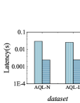
(a) Embedding Store Comparison

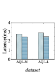
(b) Offline Training Comparison

Figure 10. The results of scalability study.

Table 3. Results of optimizing.

	pre-opt		post-opt		$\downarrow$mean	$\downarrow$ std
	mean	std	mean	std
All cases	1.692	0.120	0.620	0.004	2.7	33.4
No loop	0.654	0.012	0.519	0.003	1.3	4.6
With loop	2.136	0.166	0.663	0.004	3.2	41.5

9. Related Work

We provide an overview of the related works, including automatic workload analysis, query optimization, automatic database analysis, and pre-trained foundation models.

Workload analysis. Analyzing and understanding workloads is essential for properly designing, provisioning and optimizing services (Jain et al., 2018; Le and Mikolov, 2014; Tang et al., 2022; Kenton and Toutanova, 2019; Tran et al., 2015; Deep et al., 2020; Psallidas et al., 2022; Zhu et al., 2021). There is recent work on exploiting workload characteristics in cloud DBMSs from the query level (Psallidas et al., 2022) and the system level (Zhu et al., 2021). Although some work on workload characterization analyzes SQL logs (Paul et al., 2021; Jain et al., 2018; Tang et al., 2022; Zolaktaf et al., 2020), most of them focus on the interior of a single SQL statement. Query2Vec (Jain et al., 2018) implements a vector representation of SQL queries with natural language processing (NLP) methods, to support workload analysis tasks using a corpus. PreQR (Tang et al., 2022) improves BERT (Kenton and Toutanova, 2019) by taking into account the specific database information to learn query features and transforms human written texts into SQL queries.

As a branch of workload analysis, workload pattern mining aims to discover frequent patterns in query logs. Oracle Workload Intelligence (WI) (Tran et al., 2015) proposes a Markov chain-based method for mining SQL context. However, WI cannot be applied to industry applications. This is because in such applications, queries from multiple business logics are loaded together into a query log store, making it difficult to distinguish them using WI. On the contrary, AWM employs a classifier to solve this problem. Although there are pattern mining studies targeting streaming data (Giannella et al., 2003; Jin and Agrawal, 2007), they are not applicable for discovering patterns from query logs.

Query optimization. Query optimization technologies are generally designed for optimizing single queries, by estimating the cost of query execution (Das et al., 2019) or optimizing the query execution plan with deep neural networks (Marcus et al., 2019, 2021) or Monte Carlo Tree (Zhou et al., 2021). However, they cannot optimize multiple queries.

Some studies investigate multi-query optimization from the perspective of batch processing (Giannikis et al., 2014, 2013; Eslami et al., 2019; Damasio et al., 2019), but none of them analyze the contextual characteristics of workload. To tackle this issue, AWM exploits the discovered patterns to optimize query execution.

Automatic database analysis. Automatic analysis and optimization of databases include various functions such as tuning (Duan et al., 2009), optimizing (Herodotou and Babu, 2011; Marcus et al., 2021, 2019; Zhu et al., 2022; Zhou et al., 2021), and workload management (Marcus and Papaemmanouil, 2016), which aim to improve the performance of database systems by addressing stability, scalability and etc. Some self-driving DBMSs (Pavlo et al., 2017; Li et al., 2021b) integrate these functions to automate the overall performance of database systems. However, they do not necessarily account for user behavior and business logic. AWM, on the other hand, focuses on analyzing and optimizing the database based on user behaviors and business logic through workload pattern analysis.

Pre-trained foundation models. Pre-trained foundation models (PFMs) have shown great success in various NLP tasks, by exploiting large amounts of unlabeled text data to learn common language representations  (Kenton and Toutanova, 2019; Liu et al., 2019, 2021). PFMs have been used in tasks such as sentence embedding (Reimers and Gurevych, 2019), matching (Ge et al., 2021b), and knowledge graphs (Ge et al., 2021a, 2022; Gao et al., 2022; Liu et al., 2023; Wu et al., 2023). However, these models are not directly applicable in the database domain. The reason is that they are trained on web corpus that are significantly different from SQL queries. Although PreQR (Tang et al., 2022) applies BERT to SQL statements for tasks, such as cardinality estimation and text-to-SQL transformation, it is not designed to discover workload patterns from query logs. On the other hand, AWM leverages the benefits of PFMs and is tailored for the unique characteristics of SQL queries and database workloads.

10. Conclusions

In this paper, we propose a workload pattern discovery system AWM for large-scale industry-level workload analysis in real-time. AWM is a part of the Alibaba Cloud Database Autonomous Service (DAS). Our system AWM (i) only collects data that is specified by users to protect user privacy; (ii) trains a classifier with few labels while achieve high accuracy; (iii) discovers the workload patterns logged from the user requests; and (iv) analyzes and provides strategies for optimizing those patterns. AWM is mainly composed of four modules: DCPM, OWMM, OTM, and POM. First, DCPM is applied to collect the streaming raw query logs, and encodes the raw query logs into high-dimensional feature embeddings with rich semantic contexts and execution features. Next, OWMM firstly classifies the encoded query logs by business groups, and then discovers the workload patterns effectively for each business group. Meanwhile, OTM collects labels that are shared by users and trains the classification model accordingly. Finally, AWM automatically provides clear code optimization strategies for cloud database users. Extensive experiments have been conducted on one synthetic dataset and two real-life datasets (from Alibaba Cloud Databases). Specifically, the experimental results offer the insight that comparing with the state-of-the-arts, the accuracy of pattern discovery has been improved by 66%; the latency of online inferring has been improved by 22%; and the optimization strategies offered by the system have improved the efficiency of query processing by 2.7 times.

In the future, it is of great interest to discover the relation between database performance indicators and workload patterns. Mining workload patterns has important applications, such as query optimization. This paper focuses on a specific aspect of query optimization. However, workload patterns also hold promise for integration into online anomaly detection and root cause analysis.

References

- (1)
- Alibaba Cloud (2022) Alibaba Cloud. 2022. Alibaba Cloud Databases. https://www.alibabacloud.com/product/databases
- Amazon EC (2015) Amazon EC. 2015. Amazon web services. http://aws.amazon.com/es/ec2/
- Cao et al. (2021) Wei Cao, Xiaojie Feng, Boyuan Liang, Tianyu Zhang, Yusong Gao, Yunyang Zhang, and Feifei Li. 2021. LogStore: A Cloud-Native and Multi-Tenant Log Database. In SIGMOD. 2464–2476.
- Chandra et al. (2015) Bikash Chandra, Bhupesh Chawda, Biplab Kar, KV Reddy, Shetal Shah, and S Sudarshan. 2015. Data generation for testing and grading SQL queries. VLDBJ 24, 6 (2015), 731–755.
- Chen and Guestrin (2016) Tianqi Chen and Carlos Guestrin. 2016. XGBoost: A Scalable Tree Boosting System. In KDD. 785–794.
- Conneau et al. (2020) Alexis Conneau, Kartikay Khandelwal, Naman Goyal, Vishrav Chaudhary, Guillaume Wenzek, Francisco Guzmán, Édouard Grave, Myle Ott, Luke Zettlemoyer, and Veselin Stoyanov. 2020. Unsupervised Cross-lingual Representation Learning at Scale. In ACL. 8440–8451.
- Copel et al. (2015) Marshall Copel, Julian Soh, Anthony Puca, Mike Manning, and David Gollob. 2015. Microsoft Azure: Planning, Deploying, and Managing Your Data Center in the Cloud. Apress (2015).
- Damasio et al. (2019) Guilherme Damasio, Vincent Corvinelli, Parke Godfrey, Piotr Mierzejewski, Alex Mihaylov, Jaroslaw Szlichta, and Calisto Zuzarte. 2019. Guided automated learning for query workload re-optimization. PVLDB 12, 12 (2019), 2010–2021.
- Das et al. (2019) Sudipto Das, Miroslav Grbic, Igor Ilic, Isidora Jovandic, Andrija Jovanovic, Vivek R. Narasayya, Miodrag Radulovic, Maja Stikic, Gaoxiang Xu, and Surajit Chaudhuri. 2019. Automatically Indexing Millions of Databases in Microsoft Azure SQL Database. In SIGMOD. 666–679.
- Deep et al. (2020) Shaleen Deep, Anja Gruenheid, Paraschos Koutris, Jeffrey Naughton, and Stratis Viglas. 2020. Comprehensive and efficient workload compression. PVLDB 14, 3 (2020), 418–430.
- Duan et al. (2009) Songyun Duan, Vamsidhar Thummala, and Shivnath Babu. 2009. Tuning Database Configuration Parameters with iTuned. PVLDB 2, 1 (2009), 1246–1257.
- Eslami et al. (2019) Mehrad Eslami, Yicheng Tu, Hadi Charkhgard, Zichen Xu, and Jiacheng Liu. 2019. PsiDB: A framework for batched query processing and optimization. In IEEE BigData. 6046–6048.
- Gao et al. (2022) Yunjun Gao, Xiaoze Liu, Junyang Wu, Tianyi Li, Pengfei Wang, and Lu Chen. 2022. ClusterEA: Scalable Entity Alignment with Stochastic Training and Normalized Mini-batch Similarities. In KDD. 421–431.
- Ge et al. (2021a) Congcong Ge, Xiaoze Liu, Lu Chen, Baihua Zheng, and Yunjun Gao. 2021a. Make It Easy: An Effective End-to-End Entity Alignment Framework. In SIGIR. 777–786.
- Ge et al. (2022) Congcong Ge, Xiaoze Liu, Lu Chen, Baihua Zheng, and Yunjun Gao. 2022. LargeEA: Aligning Entities for Large-scale Knowledge Graphs. PVLDB 15, 2 (2022), 237–245.
- Ge et al. (2021b) Congcong Ge, Pengfei Wang, Lu Chen, Xiaoze Liu, Baihua Zheng, and Yunjun Gao. 2021b. CollaborEM: A Self-supervised Entity Matching Framework Using Multi-features Collaboration. TKDE (2021).
- Giannella et al. (2003) Chris Giannella, Jiawei Han, Jian Pei, Xifeng Yan, and Philip S Yu. 2003. Mining frequent patterns in data streams at multiple time granularities. Next generation data mining 212 (2003), 191–212.
- Giannikis et al. (2013) Georgios Giannikis, Darko Makreshanski, Gustavo Alonso, and Donald Kossmann. 2013. Workload optimization using shareddb. In SIGMOD. 1045–1048.
- Giannikis et al. (2014) Georgios Giannikis, Darko Makreshanski, Gustavo Alonso, and Donald Kossmann. 2014. Shared workload optimization. PVLDB 7, 6 (2014), 429–440.
- Grünwald (2007) Peter D Grünwald. 2007. The minimum description length principle. MIT press.
- Herodotou and Babu (2011) Herodotos Herodotou and Shivnath Babu. 2011. Profiling, What-if Analysis, and Cost-based Optimization of MapReduce Programs. PVLDB 4, 11 (2011), 1111–1122.
- Iyer et al. (2016) Srinivasan Iyer, Ioannis Konstas, Alvin Cheung, and Luke Zettlemoyer. 2016. Summarizing source code using a neural attention model. In ACL. 2073–2083.
- Jain et al. (2018) Shrainik Jain, Bill Howe, Jiaqi Yan, and Thierry Cruanes. 2018. Query2Vec: An Evaluation of NLP Techniques for Generalized Workload Analytics. PVLDB 11, 5 (2018).
- Jin and Agrawal (2007) Ruoming Jin and Gagan Agrawal. 2007. Frequent pattern mining in data streams. In Data Streams. Springer, 61–84.
- Kennedy et al. (2015) Oliver Kennedy, Jerry Ajay, Geoffrey Challen, and Lukasz Ziarek. 2015. Pocket data: The need for TPC-MOBILE. In Technology Conference on Performance Evaluation and Benchmarking. Springer, 8–25.
- Kenton and Toutanova (2019) Jacob Devlin Ming-Wei Chang Kenton and Lee Kristina Toutanova. 2019. BERT: Pre-training of Deep Bidirectional Transformers for Language Understanding. In NAACL. 4171–4186.
- Krishnan and Gonzalez (2015) S. P. T. Krishnan and Jose L Ugia Gonzalez. 2015. Building your next big thing with google cloud platform: A guide for developers and enterprise architects. Springer.
- Kul et al. (2018) Gokhan Kul, Duc Thanh Anh Luong, Ting Xie, Varun Chandola, Oliver Kennedy, and Shambhu Upadhyaya. 2018. Similarity metrics for SQL query clustering. TKDE 30, 12 (2018), 2408–2420.
- Le and Mikolov (2014) Quoc Le and Tomas Mikolov. 2014. Distributed representations of sentences and documents. In International conference on machine learning. PMLR, 1188–1196.
- Li et al. (2021b) Guoliang Li, Xuanhe Zhou, Ji Sun, Xiang Yu, Yue Han, Lianyuan Jin, Wenbo Li, Tianqing Wang, and Shifu Li. 2021b. openGauss: An Autonomous Database System. PVLDB 14, 12 (2021), 3028–3041.
- Li et al. (2021a) Tianyi Li, Lu Chen, Christian S Jensen, and Torben Bach Pedersen. 2021a. TRACE: Real-time compression of streaming trajectories in road networks. PVLDB 14, 7 (2021), 1175–1187.
- Li et al. (2020) Tianyi Li, Ruikai Huang, Lu Chen, Christian S Jensen, and Torben Bach Pedersen. 2020. Compression of uncertain trajectories in road networks. PVLDB 13, 7 (2020), 1050–1063.
- Liu et al. (2023) Xiaoze Liu, Junyang Wu, Tianyi Li, Lu Chen, and Yunjun Gao. 2023. Unsupervised Entity Alignment for Temporal Knowledge Graphs. In WWW. 2528–2538.
- Liu et al. (2022) Xiaoze Liu, Zheng Yin, Chao Zhao, Congcong Ge, Lu Chen, Yunjun Gao, Dimeng Li, Ziting Wang, Gaozhong Liang, Jian Tan, and Feifei Li. 2022. PinSQL: Pinpoint Root Cause SQLs to Resolve Performance Issues in Cloud Databases. In ICDE. 2549–2561.
- Liu et al. (2019) Yinhan Liu, Myle Ott, Naman Goyal, Jingfei Du, Mandar Joshi, Danqi Chen, Omer Levy, Mike Lewis, Luke Zettlemoyer, and Veselin Stoyanov. 2019. Roberta: A robustly optimized bert pretraining approach. arXiv preprint arXiv:1907.11692 (2019).
- Liu et al. (2021) Yang Liu, Yao Zhang, Yixin Wang, Feng Hou, Jin Yuan, Jiang Tian, Yang Zhang, Zhongchao Shi, Jianping Fan, and Zhiqiang He. 2021. A Survey of Visual Transformers. CoRR abs/2111.06091 (2021).
- Ma et al. (2018) Lin Ma, Dana Van Aken, Ahmed Hefny, Gustavo Mezerhane, Andrew Pavlo, and Geoffrey J. Gordon. 2018. Query-based Workload Forecasting for Self-Driving Database Management Systems. In SIGMOD. 631–645.
- Ma et al. (2020) Minghua Ma, Zheng Yin, Shenglin Zhang, Sheng Wang, Christopher Zheng, Xinhao Jiang, Hanwen Hu, Cheng Luo, Yilin Li, Nengjun Qiu, Feifei Li, Changcheng Chen, and Dan Pei. 2020. Diagnosing Root Causes of Intermittent Slow Queries in Large-Scale Cloud Databases. PVLDB 13, 8 (2020), 1176–1189.
- Marcus et al. (2021) Ryan Marcus, Parimarjan Negi, Hongzi Mao, Nesime Tatbul, Mohammad Alizadeh, and Tim Kraska. 2021. Bao: Making Learned Query Optimization Practical. In SIGMOD. 1275–1288.
- Marcus and Papaemmanouil (2016) Ryan Marcus and Olga Papaemmanouil. 2016. WiSeDB: A Learning-based Workload Management Advisor for Cloud Databases. PVLDB 9, 10 (2016), 780–791.
- Marcus et al. (2019) Ryan C. Marcus, Parimarjan Negi, Hongzi Mao, Chi Zhang, Mohammad Alizadeh, Tim Kraska, Olga Papaemmanouil, and Nesime Tatbul. 2019. Neo: A Learned Query Optimizer. PVLDB 12, 11 (2019), 1705–1718.
- Mozafari et al. (2013) Barzan Mozafari, Carlo Curino, Alekh Jindal, and Samuel Madden. 2013. Performance and resource modeling in highly-concurrent OLTP workloads. In SIGMOD. 301–312.
- MySQL 8.0 Reference Manual (2022) MySQL 8.0 Reference Manual. 2022. Performance Schema Statement Digests and Sampling. https://dev.mysql.com/doc/refman/8.0/en/performance-schema-statement-digests.html
- Nadareishvili et al. (2016) Irakli Nadareishvili, Ronnie Mitra, Matt McLarty, and Mike Amundsen. 2016. Microservice architecture: aligning principles, practices, and culture. " O’Reilly Media, Inc.".
- Paul et al. (2021) Debjyoti Paul, Jie Cao, Feifei Li, and Vivek Srikumar. 2021. Database workload characterization with query plan encoders. PVLDB 15, 4 (2021), 923–935.
- Pavlo et al. (2017) Andrew Pavlo, Gustavo Angulo, Joy Arulraj, Haibin Lin, Jiexi Lin, Lin Ma, Prashanth Menon, Todd C. Mowry, Matthew Perron, Ian Quah, Siddharth Santurkar, Anthony Tomasic, Skye Toor, Dana Van Aken, Ziqi Wang, Yingjun Wu, Ran Xian, and Tieying Zhang. 2017. Self-Driving Database Management Systems. In CIDR.
- Psallidas et al. (2022) Fotis Psallidas, Ashvin Agrawal, Chandru Sugunan, Khaled Ibrahim, Konstantinos Karanasos, Jesús Camacho-Rodríguez, Avrilia Floratou, Carlo Curino, and Raghu Ramakrishnan. 2022. OneProvenance: Efficient Extraction of Dynamic Coarse-Grained Provenance from Database Logs. arXiv preprint arXiv:2210.14047 (2022).
- Reimers and Gurevych (2019) Nils Reimers and Iryna Gurevych. 2019. Sentence-BERT: Sentence Embeddings using Siamese BERT-Networks. In EMNLP. 3980–3990.
- Richardson and Ruby (2008) Leonard Richardson and Sam Ruby. 2008. RESTful web services. " O’Reilly Media, Inc.".
- Tang et al. (2022) Xiu Tang, Sai Wu, Mingli Song, Shanshan Ying, Feifei Li, and Gang Chen. 2022. PreQR: Pre-training Representation for SQL Understanding. In SIGMOD. 204–216.
- Theriault and Heney (1998) Marlene Theriault and William Heney. 1998. Oracle Security. O’Reilly & Associates, Inc.
- Tran et al. (2015) Quoc Trung Tran, Konstantinos Morfonios, and Neoklis Polyzotis. 2015. Oracle Workload Intelligence. In SIGMOD. 1669–1681.
- Verbitski et al. (2017) Alexandre Verbitski, Anurag Gupta, Debanjan Saha, Murali Brahmadesam, Kamal Gupta, Raman Mittal, Sailesh Krishnamurthy, Sandor Maurice, Tengiz Kharatishvili, and Xiaofeng Bao. 2017. Amazon aurora: Design considerations for high throughput cloud-native relational databases. In SIGMOD. 1041–1052.
- Wu et al. (2023) Junyang Wu, Tianyi Li, Lu Chen, Yunjun Gao, and Zhiheng Wei. 2023. SEA: A Scalable Entity Alignment System. In The 46th International ACM SIGIR Conference on Research and Development in Information Retrieval.
- Yoon et al. (2016) Dong Young Yoon, Ning Niu, and Barzan Mozafari. 2016. DBSherlock: A Performance Diagnostic Tool for Transactional Databases. In SIGMOD. 1599–1614.
- Zhou et al. (2021) Xuanhe Zhou, Guoliang Li, Chengliang Chai, and Jianhua Feng. 2021. A Learned Query Rewrite System using Monte Carlo Tree Search. PVLDB 15, 1 (2021), 46–58.
- Zhu et al. (2022) Rong Zhu, Ziniu Wu, Chengliang Chai, Andreas Pfadler, Bolin Ding, Guoliang Li, and Jingren Zhou. 2022. Learned Query Optimizer: At the Forefront of AI-Driven Databases. In EDBT. 1–4.
- Zhu et al. (2021) Yiwen Zhu, Subru Krishnan, Konstantinos Karanasos, Isha Tarte, Conor Power, Abhishek Modi, Manoj Kumar, Deli Zhang, Kartheek Muthyala, Nick Jurgens, et al. 2021. Kea: Tuning an exabyte-scale data infrastructure. In SIGMOD. 2667–2680.
- Zolaktaf et al. (2020) Zainab Zolaktaf, Mostafa Milani, and Rachel Pottinger. 2020. Facilitating SQL query composition and analysis. In SIGMOD. 209–224.