Federated Epidemic Surveillance

Abstract

The surveillance of a pandemic is a challenging task, especially when crucial data is distributed and stakeholders cannot or are unwilling to share. To overcome this obstacle, federated methodologies should be developed to incorporate less sensitive evidence that entities are willing to provide. This study aims to explore the feasibility of pushing hypothesis tests behind each custodian’s firewall and then meta-analysis to combine the results, and to determine the optimal approach for reconstructing the hypothesis test and optimizing the inference. We propose a hypothesis testing framework to identify a surge in the indicators and conduct power analyses and experiments on real and semi-synthetic data to showcase the properties of our proposed hypothesis test and suggest suitable methods for combining $p$-values. Our findings highlight the potential of using $p$-value combination as a federated methodology for pandemic surveillance and provide valuable insights into integrating available data sources.

1 Introduction

The prompt detection of outbreaks is critical for public health authorities to take timely and effective measures. Providing early warning, whether regarding the emergence of a new pathogen or a renewed wave of an existing epidemic, allows for preparatory action either to reduce transmission or to prepare for increased load on the health system. Nonetheless, real-time surveillance is challenging, particularly in countries such as the United States where relevant data is typically held by many separate entities such as hospitals, laboratories, insurers and local governments. These entities are often unable or unwilling to routinely share data for a variety of reasons including patient privacy, regulatory compliance, competitiveness and commercial value. Accordingly, creating effective surveillance pipelines currently require public health authorities to mandate reporting for particular conditions of interest. This process is both cumbersome and reactive: a new reporting pipeline cannot be created until well into a public health emergency.

We propose and evaluate the feasibility of an alternative approach that we refer to as federated epidemic surveillance. The core concept is that health information, including even aggregate counts, never leaves the systems of individual data custodians. Rather, each custodian shares only specified statistics of their data, for example, the $p$-value from a specified hypothesis test. These statistics are then aggregated to detect trends that represent potential new outbreaks. Leveraging inputs from a variety of data custodians provides significantly improved statistical power: trends which are only weakly evident in any individual dataset may be much more apparent if data could be pooled together. To illustrate, consider COVID-19 hospitalizations in Seattle reported by four facilities to the US Department of Health & Human Services (HHS), as shown in Figure 1. As the trends observed at different facilities vary substantially, it would be difficult to catch the overall increase by looking at any single facility. However, if the combined data from all facilities are available, a rapid increase in hospitalizations is clearly visible starting in March. Our goal is to detect outbreaks with comparable statistical power as if the data could be pooled together, but without individual data providers disclosing even their time series of counts.

Our analysis reveals that federated surveillance is indeed possible, often attaining performance similar to that possible with fully centralized data. We analyze a simple two-step approach: first, conduct separate hypothesis tests on the occurrence of a “surge" at different sites and subsequently use a meta-analysis framework to combine the resulting $p$-values into a single hypothesis test for an outbreak. More elaborate approaches (e.g. based on homomorphic computation or other cryptographic techniques) could allow more sophisticated computations under strong privacy guarantees. However, our goal is to demonstrate that high-performance federated surveillance is achievable using even simple, easily implementable methods. Our results indicate that effective epidemic surveillance is possible even in environments with decentralized data, and provide a roadmap towards modernizing surveillance systems in preparation for current and future public health threats.

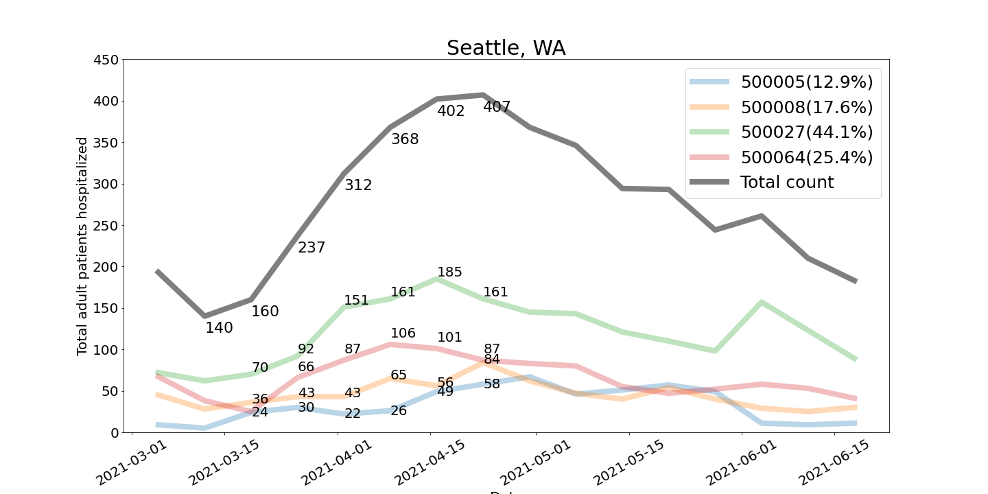
Figure 1: Adult patients hospitalized with confirmed COVID (7 day sum) of different facilities in Seattle

Before delving into the details of the framework, a concise introduction to the notations employed in this article is provided in Appendix Section 1.

2 Results

We explore the potential for simple federated surveillance methods to detect surges in a condition of interest using a variety of real and semisynthetic data. To start, we more formally introduce our objective. Precisely defining what constitutes a surge or outbreak is difficult. We operationalize a surge as sufficiently large increase in the rate of new cases over a specified length of time. Formally, we model the time series $k_{t}$ of interest (e.g., cases or hospitalizations with a particular condition) as following a Poisson process $k_{t}\sim Poi(\lambda_{t})$ for some time-varying rate parameter $\lambda_{t}$. At a testing time $T$, we compare to a baseline period $T-\ell...T-1$ and say that a surge occurs when the rate increases by at least a factor of $\theta$ during the testing period compared to the baseline period. For simplicity, we model counts in the baseline period as following a Poisson distribution with a constant parameter $\lambda_{B}$: $k_{Bj}\sim Poi(\lambda_{B}),j=T-\ell...T-1$. Similarly, during the testing period, we model $k_{T}\sim Poi(\lambda_{T})$ for a new parameter $\lambda_{T}$. We say that a surge occurs when $\frac{\lambda_{T}}{\lambda_{B}}>1+\theta$. We will analyze methods which test this hypothesis using the realized time series $k_{t}$, effectively asking whether a rise in counts must be attributed to a rise in the rate of new cases or whether it could be explained by Poisson-distributed noise in observations instead. Importantly, none of our results rely on the assumption that the data actually follows this generative process; indeed, we will evaluate using real epidemiological time series where such assumptions are not satisfied. Rather, our aim is to show that decentralized versions of even this simplified hypothesis test can successfully detect surges.

Formally, we test the null hypothesis that the Poisson rate ratio $\frac{\lambda_{T}}{\lambda_{B}}$ is not larger than $1+\theta$. We apply the uniformly most powerful (UMP) unbiased test for this hypothesis (Lehmann et al., 2005; Fay, 2014), which has the $p$-value $Pr[r\geq k_{T}]$ where $r$ is a Binomial random variable $r\sim Bin(\sum_{j=1}^{l}k_{Bj}+k_{T},\frac{1+\theta}{1+\theta+l})$. That is to, calculate the $p$-value of the Binomial test, we sum up the probabilities of observing more extreme values than $k_{T}$ if counts were uniformly split between the baseline and test periods. Section 4.1 includes more details about the hypothesis test.

In the federated setting, each data custodian computes $p$-values for this hypothesis test using only their own time series. The $p$-values are then combined using methods from meta-analysis. (See Section 4.2 for more discussions.) Considering $p_{1},\dots,p_{n}$ are $p$-values obtained from $n$ independent hypothesis tests and the joint null hypothesis for the $p$-values is $H_{0}:p_{i}\sim U[0,1],i=1,\dots,N$ (Heard and Rubin-Delanchy, 2018), several commonly used statistics and their corresponding distributions can be computed accordingly. We listed some popular ones in Table 1.

Methods	Statistics	Distributions under the null
Stouffer’s	$\sum_{i=1}^{N}\Phi^{-1}(p_{i})$	$N(0,N)$
Fisher’s	$-2\sum_{i=1}^{N}\log p_{i}$	$\chi^{2}_{2N}$
Pearson’s	$-2\sum_{i=1}^{N}\log(1-p_{i})$	$\chi^{2}_{2N}$
Tippett’s	$min\{p_{1},\dots,p_{N}\}$	$Beta(1,N)$

Table 1: Common meta-analysis methods

2.1 Efficacy of Federated Surveillance

We start by studying the statistical power and sensitivity of federated surveillance methods compared to centralized data, i.e., whether decentralized hypothesis tests allow comparable accuracy in detecting surges compared to the (unattainable) ideal setting where all data could be pooled for a single test. We assess decentralized methods using both their theoretical expected accuracy on data drawn from our simplified generative model and on two real Covid-19 datasets.

Figure 2 shows the expected statistical power of each meta-analytic method for combining $p$-values on data drawn from our generative model, compared to the statistical power of a centralized version of the same hypothesis test and to a version which uses only the counts from a single data provider. We fix a threshold of $\theta=0.3$ for a surge. The $x$ axis varies the true rate of growth under the alternative hypothesis, with higher power to detect surges when they deviate more significantly from the null. To ensure a fair comparison, we calibrate the rejection threshold for each method to match the nominal $\alpha=0.05$ rejection rate when the true growth rate is exactly 30% (i.e., precisely satisfying the null). We simulate a total of 200 counts distributed between 2 sites (Figure 2(a)) and 8 sites (Figure 2(b)).

We find that, in this idealized setting, the top-performing federated method (Stouffer’s method) almost exactly matches the power of the centralized-data test. Conversely, significant power is lost by using only the $p$-value from a single site, indicating that sharing information across sites is necessary for good performance. The other meta-analytic methods exhibit lower power; in later sections, we will examine the settings in which different meta-analytic methods for combining the $p$ values lead to better or worse performance.

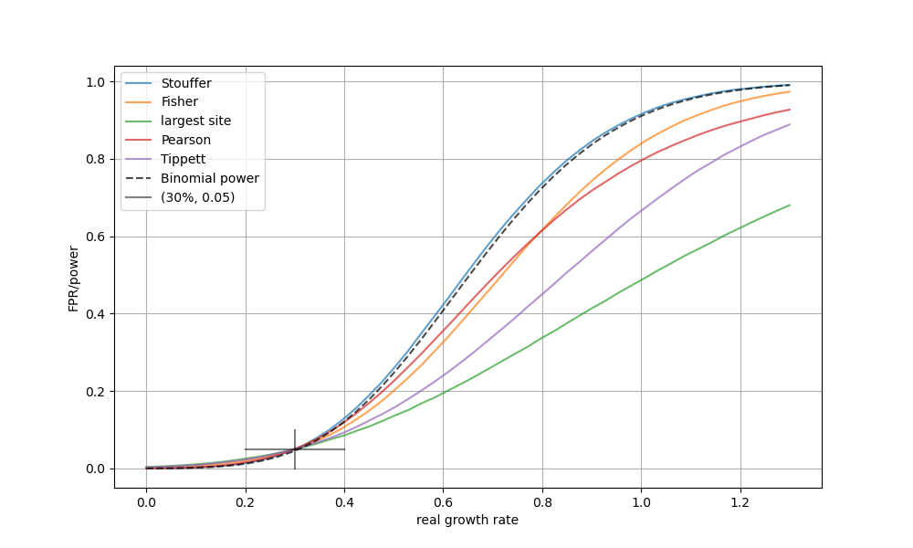
(a)

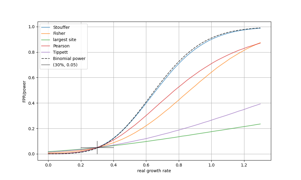
(b)

Figure 2: Power analysis of the naive methods.

In order to validate the robustness of different methods in the real world, we utilize two real datasets. These datasets provide a more realistic representation of the complexities and challenges encountered in real-world scenarios, allowing us to assess the performance of the methods under more diverse conditions. The data we use are (1) The "COVID-19 Reported Patient Impact and Hospital Capacity by Facility" dataset, obtained through the Delphi Epidata API (Farrow et al., 2015), covers the period from 2020-07-10 to 2023-03-03. This dataset provides facility-level data on a weekly basis and primarily includes the "total adult patients hospitalized" metric for case counts. (2) The "Counts of claims with confirmed COVID-19" dataset provided by Change Healthcare covering the period from 2020-08-02 to 2022-07-30. This dataset provides county-level claim data on a daily basis. More information about the real data is put in Appendix Section 4.

In our real data analysis, we utilize hospitalization data at the facility level to generate county-level alarms based on the $p$-values, as well as claim data at the county level to create alarms. The term "alarm" in this context signifies the occurrence of something suspicious or noteworthy. In this particular case, the alarm indicates that the confidence level of rejecting the null hypothesis is below a predetermined threshold $\alpha=0.05$. For more details of evaluation, see Section 4.5. Due to variations in reporting frequency and the number of sites, the hospitalization data tends to have larger counts distributed in fewer sites, while the claim data has smaller counts distributed in more sites. Based on our previous discussion, we anticipate that Stouffer’s method would be more suitable for the hospitalization data, while Fisher’s method would be better suited for the claim data. By applying these naive meta-analysis methods to our two datasets, we obtain the recall-precision curves as Figure 3. The results demonstrate that the federated test, with appropriate method selection, can effectively reconstruct centralized information, as indicated by F1 scores greater than 0.9 for both datasets. On the other hand, relying solely on the single largest facility yields suboptimal results. Furthermore, the selection of the optimal combination method aligns with our expectations.

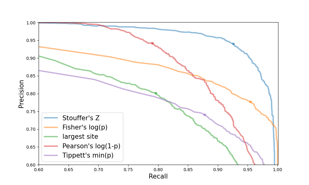
(a)

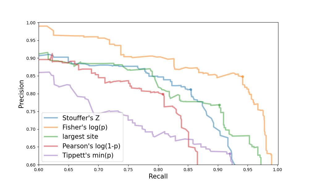
(b)

Figure 3: Real data analysis of the naive methods.

2.2 How Different Settings Influence the Surveillance

Based on our discussion on theoretical analysis (see Section 4) and the experiments on the real-world data above, we have drawn preliminary conclusions regarding our proposed test. Firstly, employing a combined test using a meta-analysis framework generally yields superior performance compared to relying solely on a single entity, even if the entity contributes a significant portion of the counts. Secondly, the optimal choice of method depends on specific features of the data. If the reported counts are less distributed and have relatively large magnitudes, Stouffer’s method is preferable. However, if the counts are more evenly distributed, it is better to consider $\log p$-based Fisher’s method.

To gain a comprehensive understanding of the impact of various properties on the combination process, it is beneficial to selectively modify one factor while keeping others constant. However, it is important to note that the settings encompass multiple dimensions of variation. Firstly, as the number of entities in a region increases, combining the data becomes more challenging due to the accumulation of combination errors. Secondly, the magnitude of counts $n$ influences the selection of $p$-value combination methods, as evident from the power formula in Equation 7. Thirdly, the imbalance in the shares of different sites challenges the robustness of the combination methods.

To conduct a rigorous analysis of these factors while effectively controlling for other variables, we employ a semi-synthetic data analysis (see Section 4.6) utilizing real COVID-related claims data reported on a weekly basis. The underlying prevalence of the Poisson-distributed counts is estimated by applying a moving average smoother to the real data. Simulated observations are then generated, assuming the observed data follows a Poisson distribution with the smoothed data as the rate parameter. This approach enables us to investigate the systematic errors resulting from noise in both centralized and federated settings, as well as compare the performance of different combination methods in the presence of this noise.

In Figure 4, each plot represents an analysis where one dimension is varied while keeping the others fixed. Figure 4(a) focuses on changing the number of sites while maintaining equal shares among them. Figure 4(b) incorporates a multiplier to the underlying prevalence, allowing us to examine the influence of the magnitude of the counts. Figure 4(c) explores the case where the number of sites is fixed at $N=5$, and the degree of imbalance in the shares is varied. The level of imbalance is quantified using the normalized entropy metric $S=\frac{-\sum_{i=1}^{N}s_{i}\log s_{i}}{\log N}$, where a value of 1 indicates perfectly equal shares.

Our findings indicate that federated analysis performs well compared to the centralized setting. However, relying solely on a single facility, even with a relatively large share of the counts, yields poor results. Fisher’s method demonstrates the highest stability when the number of sites varies in an equal-shared setting. Therefore, when the data is highly distributed among numerous sites, Fisher’s method is the preferred choice for analysis. Additionally, we observe that Fisher’s method performs slightly better when the magnitude of the reports is relatively small. Furthermore, our analysis suggests that selecting the largest site as the representative can outperform naive combination methods only when there is one dominant site in the entire region, as indicated by a normalized entropy of less than 0.7 and the largest site having a share of 65%.

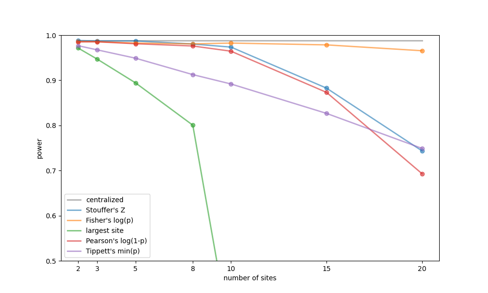
(a)

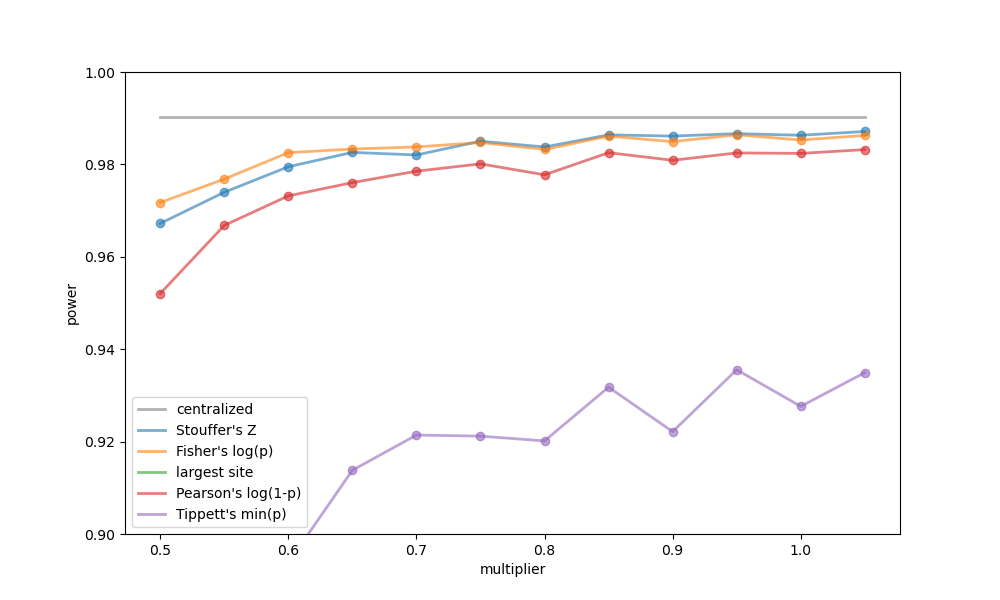
(b)

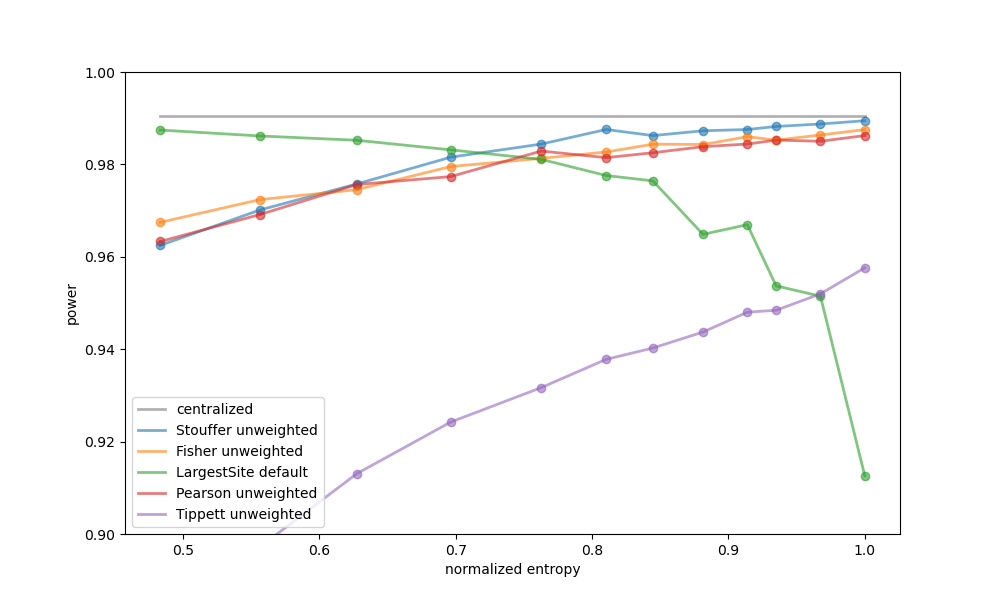
(c)

Figure 4: Semi-synthetic data analysis of the naive methods.

2.3 Enhancing Federated Surveillance with Auxiliary Information

In the context of meta-analysis, most discussions and methodologies assume that $p$-values are uniformly distributed under the null hypothesis. However, this assumption does not hold in many cases (as discussed in Section 4). In light of this, we can explicitly formulate the equations for $p$-values and explore an alternative perspective on meta-analysis: the approximation of $p$-values and the subsequent combination of these approximations.

It is clear that directly combining the $p$-values of different sites from $p$-values of entities (Equation 8) to $p$-value of the summation of their counts (Equation 6) without any loss is not possible. Therefore, our goal is to find better approximations and develop improved methods for combining the approximations. The choice between different meta-analysis methods is analog to choosing a better approximation. However, we can incorporate estimated shares of different data providers and assign weights to the studies, as weighting is a common approach for integrating evidence (Hou and Yang, 2022; Zhang and Wu, 2022; Vovk and Wang, 2020; Whitlock, 2005). Based on our analysis in Section 4, we have concluded that the optimal weights for combining Stouffer’s method are the square roots of the shares. In other words, it’s formulated as Equation 1.

$$p=\Phi\left(\sum_{i=1}^{N}\sqrt{s_{i}}\Phi^{-1}(p_{i})\right)$$ (1)

where $p$ and $p_{i}$ are combined and distributed $p$-values.

For Fisher’s method, we have observed that the $wFisher$ method proposed by Yoon et al. (Yoon et al., 2021) is the most stable. In this method, they assign weights to the degrees of freedom (DFs) of the Gamma distribution based on the shares and control the total DFs to match that of the naive Fisher’s method. Specifically, they formulate the framework as Equation 2.

$$p=1-F_{\chi^{2}_{2N}}\left(\sum_{i=1}^{N}F^{-1}_{Gam(\frac{s_{i}N}{2},\frac{1}{2})}(1-p_{i})\right)$$ (2)

The power curves of Appendix Section 3 Figure 2 demonstrate that both Fisher’s method and Stouffer’s method exhibit improvement upon the inclusion of weights. Notably, Stouffer’s method demonstrates the ability to closely approximate the centralized Binomial power curve even in highly unbalanced scenarios. Moreover, even in the extremely unbalanced setting, the largest site alone fails to achieve a significantly high test power.

In addition to adding weights, we can make a further modification to Stouffer’s method if we have estimates of the total reports of all sites $n=\sum_{i=1}^{N}n_{i}$. The modification involves incorporating a continuity correction term to make the results less conservative, which can be particularly useful when the total counts are small. The modified method can be expressed as Equation 3.

$$p=\Phi\left(\sum_{i=1}^{N}\sqrt{s_{i}}\Phi^{-1}(p_{i})+\frac{1-N}{2\sqrt{\rho(1-\rho)n}}\right)$$ (3)

By comparing the performance of selecting the largest site with Stouffer’s and Fisher’s methods before and after the modifications, using our semi-synthetic data analysis framework, we can observe that after adding weights, both methods show improvements. Furthermore, the combined methods outperform selecting the largest site, even in extreme settings where the largest site among all five accounts for 80% of the share. Specifically, the weighted Stouffer’s method closely approximates the performance of the centralized setting when the shares between sites are similar, while wFisher demonstrates stability across different share settings.

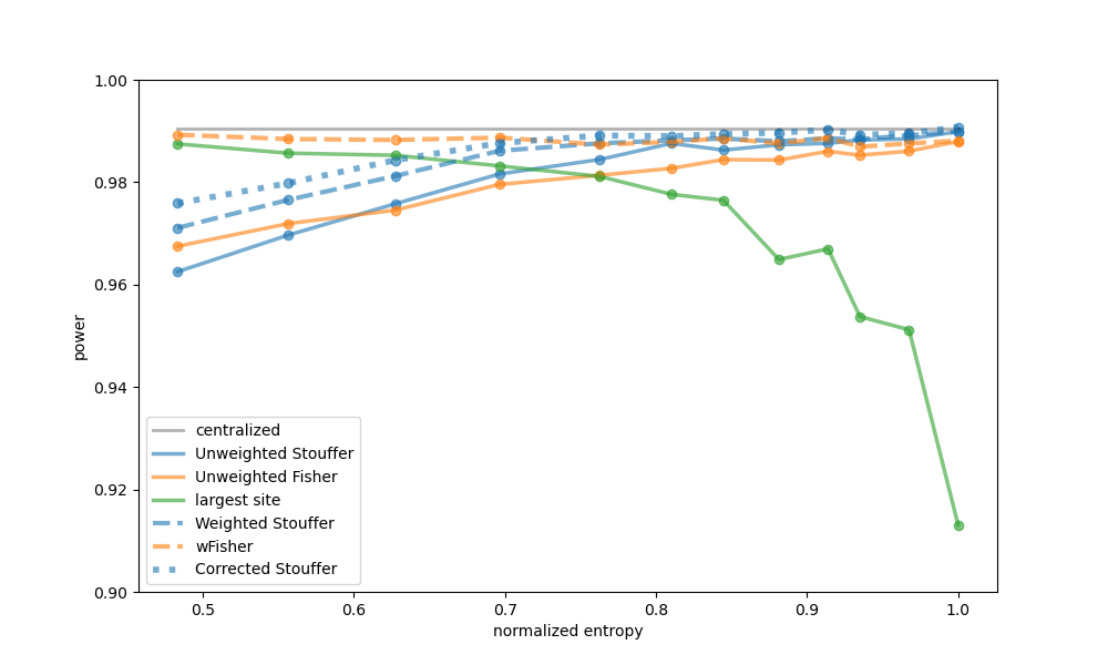
Figure 5: Semi-synthetic analysis of the modified methods.

However, in real-time scenarios, the share of different sites may not be readily available, necessitating the training and updating of weights in our framework. Various approaches can be employed depending on the accessibility of information. One option is to utilize coarse-grained reports with lags. By incorporating such information, the accuracy of generating alarms can be improved, provided that a reasonable training scheme is implemented. The impact of the reporting cycle and lag of the auxiliary information on the performance of adding weights in real datasets is illustrated in Appendix Section 5 Figure 4. Generally speaking, these factors have minimal influence on the improvement achieved through weighted combinations. Another viable option is the integration of auxiliary information, such as bed usage and ICU data, which has the potential to further improve performance as well. The details of this integration can be found in Appendix Section 5.

The performance of both the naive and modified versions of Stouffer’s and Fisher’s methods is depicted in Figure 6. As anticipated, the weighted versions of both methods show improvement. Additionally, the inclusion of continuity correction proves beneficial for daily-reported claim data with smaller counts. Conversely, for weekly-reported hospitalization data with larger counts, continuity correction does not significantly impact the results.

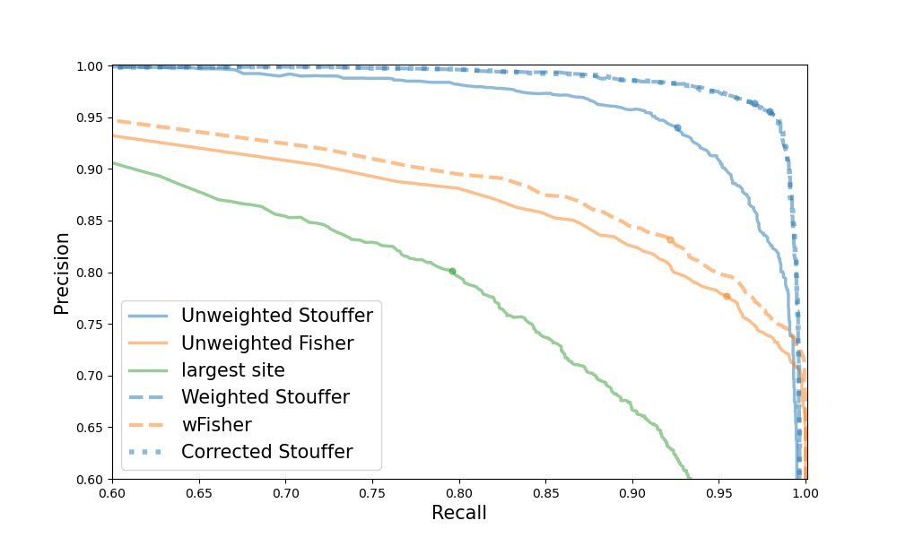
(a)

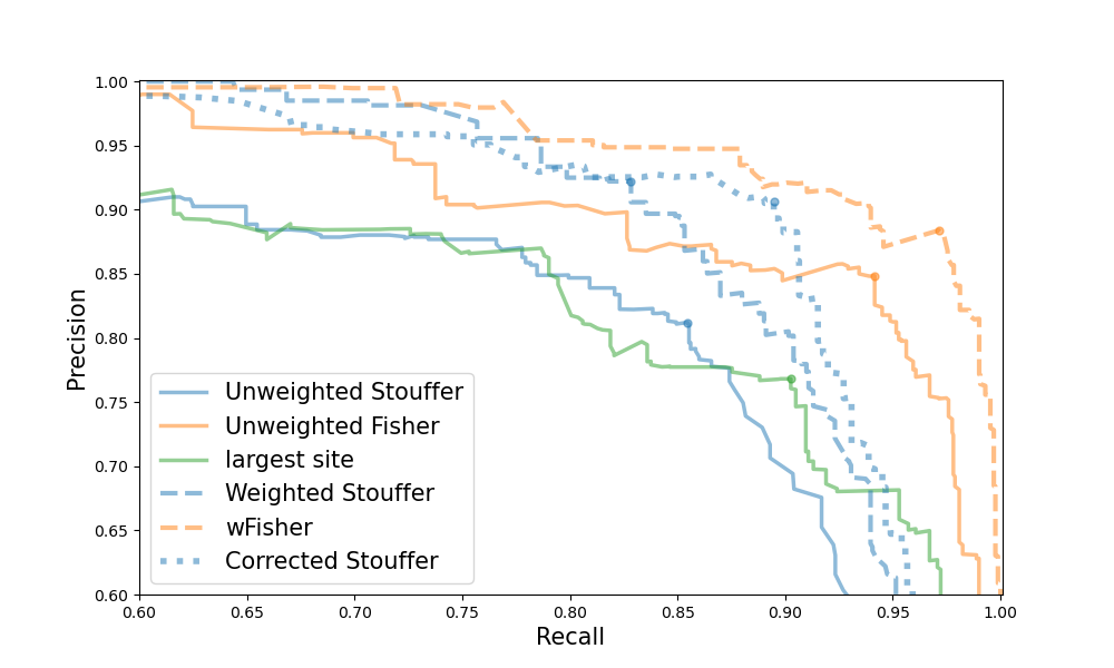
(b)

Figure 6: Real data analysis of the modified methods.

In conclusion, in most cases, adding weights to the combination of $p$-values can be beneficial, provided that the weights are accurately estimated. When the magnitudes of the reports are relatively small, incorporating continuity correction, if feasible, can help make the test less conservative.

3 Discussion

The surveillance of pandemics presents significant challenges, especially when crucial data is distributed and stakeholders are unwilling or unable to share it. In this study, we have introduced a federated methodology for pandemic surveillance, which involves conducting hypothesis tests behind each custodian’s firewall and subsequently performing a meta-analysis to combine the results. Through power analyses and experiments using real and semi-synthetic data, we have demonstrated the feasibility and effectiveness of our proposed hypothesis testing framework.

Our study’s results have shown the effectiveness of the suggested hypothesis testing framework in identifying surges in the indicators assumed to follow a Poisson distribution. This framework offers a statistical method for determining whether the rate increase surpasses a user-defined threshold. By utilizing $p$-values, we have been able to combine results from multiple sites while addressing privacy concerns, as $p$-values alone do not pose a significant risk of privacy leakage. Furthermore, our findings have indicated that the choice of combination method in meta-analysis depends on the data’s characteristics. Stouffer’s method is more suitable for less distributed data with a larger magnitude of reports, while Fisher’s method performs better in a more distributed and unbalanced setting. Moreover, if we have access to additional information about the entities’ shares and even the estimated total counts in a given region, we can further enhance our evidence combination and achieve results that are almost as good as those in a centralized setting.

However, our study has several potential extensions that warrant further investigation. Firstly, our focus has been primarily on detecting surges in indicators assumed to follow a Poisson distribution, which may not capture the full spectrum of pandemic surveillance needs. Exploring the detection of other patterns and developing integrated statistical models for multiple indicators would improve the accuracy and timeliness of surveillance efforts. Additionally, addressing the challenges of defining privacy boundaries and establishing consensus on data-sharing protocols remains an ongoing obstacle that requires attention.

In conclusion, our findings underscore the potential of utilizing $p$-value combination as a federated methodology for pandemic surveillance. By leveraging less sensitive evidence from multiple custodians, we can overcome the challenges posed by data distribution and privacy concerns. Our proposed framework enables the rapid detection of surges and the integration of available data sources, empowering health authorities to take prompt and effective measures in response to epidemic outbreaks.

4 Methods

4.1 Poisson rate ratio test for detecting a surge

As the simplest idea, the Poisson distribution is employed to model disease indicators expressed as count data concerning additivity. The Poisson distribution characterizes the probability of the number of occurrences within a fixed interval, assuming a constant mean rate and independent occurrences (Cox, 1955). The Poisson rate parameter $\lambda$ serves as both the expectation and variance of the distribution of $k$. In a short time period such as a week or a month, if there is no surge, the counts of a certain indicator follow a Poisson distribution with a fixed rate parameter $\lambda$, which can be estimated based on observations from the previous period. However, in the presence of a sudden surge, the distribution changes, and the rate parameter $\lambda$ increases.

By monitoring and analyzing the changes, we can effectively identify the occurrence of a surge. To achieve this, we propose conducting a hypothesis test to determine whether the increase in Poisson rates exceeds a user-defined threshold, denoted as $\theta$. This threshold can be tailored to the inherent characteristics of different indicators, allowing for adaptive control of the false discovery rate. Specifically, a surge is defined as a Poisson rate that increases by at least $\theta$ during the testing period with Poisson rate parameter $\lambda_{T}$, compared to the baseline period with parameter $\lambda_{B}$, shown as Equation 4.

$$H_{0}:\frac{\lambda_{T}}{\lambda_{B}}\leq 1+\theta$$ (4)

We propose utilizing the UMP unbiased test, which is a conditional method of testing two Poisson rates ratio first proposed by Przyborowski and Wilenski (Przyborowski and Wilenski, 1940), shown as Equation 5. The traditional conditional test is known for being exact while conservative, as the actual significance level is always below the nominal level (Gu et al., 2008).

$$H^{\prime}_{0}:\frac{\lambda_{T}}{\lambda_{T}+l\lambda_{B}}\leq\frac{1+\theta}{1+\theta+l}$$ (5)

Essentially, the UMP test corresponds to a Binomial test that examines the indicator during the testing period conditioning on the total counts of both the baseline and testing periods. Using this test, we can easily determine the $p$-value through a one-tailed exact test. The formulation of the $p$-value is shown as Equation 6.

$$\begin{split}p&=Pr(r\geq k_{T}|\sum_{j=1}^{l}k_{Bj}+k_{T},\frac{1+\theta}{1+\theta+l})\\ &=\sum_{r=0}^{c}\tbinom{n}{r}(1-\rho)^{{n}-r}\rho^{r}\end{split}$$ (6)

where $c:=\sum_{j=1}^{l}k_{Bj},n:=\sum_{j=1}^{l}k_{Bj}+k_{T},\rho:=\frac{l}{1+\theta+l}$.

The power of a hypothesis test is defined as the probability of rejecting the null hypothesis in favor of a specific alternative hypothesis. It measures the test’s ability to distinguish between the null hypothesis and a particular alternative hypothesis. In the case of the Binomial test under the null hypothesis, we need to determine the critical value $k_{cr}$ for $k_{T}$ at a given type I error rate $\alpha$. This critical value represents the minimum number of successes in the sample required to reject the null hypothesis in favor of the alternative hypothesis. Mathematically, the critical value is determined by finding $k_{cr}$ that satisfies the condition $Pr(r\geq k_{cr}|n=\sum_{j=1}^{l}k_{Bj}+k_{T},\frac{1+\theta}{1+\theta+l})\leq\alpha$. Under the alternative hypothesis, characterized by a higher growth rate of the Poisson rate $\theta^{\prime}>\theta$, the power is computed as $Pr(r\geq k_{cr}|n=\sum_{j=1}^{l}k_{Bj}+k_{T},\frac{1+\theta^{\prime}}{1+\theta^{\prime}+l})$. The power quantifies the test’s ability to detect a surge when it truly exists.

The analytical formula for calculating power in the discrete distribution is hard to use. As a practical alternative, a Gaussian approximation of Binomial distribution with continuity correction can be employed. This approximation is effective by ruling out the rounding errors on the power calculation while maintaining an acceptable level of precision. With continuity correction, we can compute the power as Equation 7. (See Appendix Section 2 for details.)

$$\text{power}=\Phi(\frac{\sqrt{nl}(\theta^{\prime}-\theta)}{(1+\theta+l)\sqrt{(1+\theta^{\prime})}}-\frac{Z_{\alpha}(1+\theta^{\prime}+l)\sqrt{1+\theta}}{(1+\theta+l)\sqrt{(1+\theta^{\prime})}}-\frac{1+\theta^{\prime}+l}{2\sqrt{nl(1+\theta^{\prime})}})\\$$ (7)

The expression inside the $\Phi(\cdot)$ function comprises three terms, each capturing a specific aspect of the analysis. The first term quantifies the impact of the total counts’ magnitude, while the second term relates to the type I error rate. The third term corresponds to the continuity correction term, which can be ignored when the sample size $n$ is sufficiently large. This formula provides an approximation of the power and allows for a more intuitive understanding of the influence of different parameters.

4.2 Overview of meta-analysis methods

Meta-analysis is known for its ability to enhance statistical power by combining signals of moderate significance, effectively controlling false positives, and enabling comparisons and contrasts across tests and time (Yoon et al., 2021). The properties of various $p$-value combination methods have been extensively studied. For instance, Heard and Rubin-Delanchy (Heard and Rubin-Delanchy, 2018) observed that Tippett’s and Fisher’s methods are more sensitive to smaller $p$-values, while Pearson’s methods are more sensitive to larger $p$-values. They also suggested that Fisher’s and Pearson’s methods are more suitable for testing positive-valued data under the alternative hypothesis, with Fisher’s method performing better for larger values and Pearson’s method for smaller values. Additionally, Stouffer’s method is often preferred for testing real-valued data that approximates a Gaussian distribution.

Among the various combination methods, Stouffer’s and Fisher’s methods have gained significant attention in the literature due to their popularity in meta-analysis. Elston (Elston, 1991) noted that Fisher’s method favors $p$-values below $\frac{1}{e}$ when the number of sites is infinite. Similarly, Stouffer’s method favors a threshold point of $\frac{1}{2}$, while Pearson’s method favors $1-\frac{1}{e}$. Rice (Rice, 1990) suggested that methods like Stouffer’s are more appropriate when all tests address the same null hypothesis as the combined $p$-value can be interpreted as a "consensus $p$-value". On the other hand, Fisher’s method is particularly useful when testing against broad alternatives. It specifically tests whether at least one component test is significant. It has shown superiority in certain scenarios, such as in Genome-wide association studies (GWAS) where there may be significant differences in effect sizes between different populations (Yoon et al., 2021). In contrast, Stouffer’s and Lancaster’s methods tend to lose power when combining more unassociated $p$-values. This highlights Fisher’s method’s advantage in handling potential negative correlations between entities, which can arise due to factors like competition.

The meta-analysis methods discussed in Table 1 rely on the assumption that the test statistics follow probability distributions that are continuous under their respective null hypotheses. Additionally, the joint null hypothesis for the $p$-values is stated as $H_{0}:p_{i}\sim U[0,1],i=1,\dots,N$ (Heard and Rubin-Delanchy, 2018). However, these assumptions do not hold for the hypothesis test proposed in our study. There are two key factors contributing to this deviation. Firstly, in the case of discrete distributions like the Binomial distribution, the $p$-values are not uniformly distributed, even under the null hypothesis. Secondly, when the null hypothesis is rejected, the distribution of $p$-values undergoes a shift, necessitating strategies to mitigate the resulting decrease in power during meta-analysis. To address these issues, we present a perspective that leverages the explicit format of the $p$-values in both centralized and distributed settings, followed by a discussion on how to combine them with minimal loss.

In the Binomial test of the distributed setting, the $p$-value for site $i$ can be expressed as Equation 8.

$$\begin{split}p_{i}&=Pr(r\geq k_{Ti}|\sum_{j=1}^{l}k_{Bij}+k_{Ti},\frac{1+\theta}{1+\theta+l})\\ &=\sum_{r=0}^{c_{i}}\tbinom{n_{i}}{r}(1-\rho)^{{n_{i}}-r}\rho^{r}\end{split}$$ (8)

where $c_{i}:=\sum_{j=1}^{l}k_{Bij},n_{i}:=\sum_{j=1}^{l}k_{Bij}+k_{Ti}$.

It is evident that directly combining the $p$-values of different sites from Equation 8 to Equation 6 without any loss is not feasible. Therefore, we delve deeper into the discussion of combination methods, specifically Stouffer’s and Fisher’s methods, within the context of the approximation then combining framework.

4.3 Stouffer’s method

Stouffer’s method is employed by utilizing the Gaussian approximation of the Binomial parameter, which is based on the central limit theorem. This approach is commonly used when analyzing the Binomial and Poisson distributions, especially when the counts are sufficiently large. To test the success probability $\rho$ using Stouffer’s method, the distribution of $\frac{c}{n}-\rho$ is approximated by $N(0,\frac{\rho(1-\rho)}{n})$. The z-score can then be calculated as $z=\frac{(c-n\rho)}{\sqrt{n\rho(1-\rho)}}$ (Brown et al., 2002). The $p$-value of the Binomial exact test is determined by the cumulative distribution function $F_{\text{Bin}}(c;n,\rho)$. Considering the rounding error or fluctuation term $\epsilon_{r}=\frac{1}{2}-\{(n\rho+z\sqrt{n\rho(1-\rho)})-\lfloor(n\rho+z\sqrt{n\rho(1-\rho)})\rfloor\}$, which takes values in the interval $[-\frac{1}{2},\frac{1}{2}]$. Thus, the $p$-value approximation with error terms can be expressed as Equation 9 (Brown et al., 2002; Bhattacharya and Rao, 2010; Esseen, 1945).

$$p=\Phi(z)+(\frac{(1-2\rho)(1-z^{2})}{6}+\epsilon_{r})\frac{\Phi(z)}{\sqrt{n\rho(1-\rho)}}+\mathbf{O}(n^{-1})$$ (9)

It should be noted that the denominator $\sqrt{n\rho(1-\rho)}$ in the first-order error term indicates that Stouffer’s method may be unreliable for small sample sizes or when the probability is close to 0 or 1 (Brown et al., 2001).

After applying the Gaussian approximations, the combination of $p$-values becomes the next focus. One limitation of the naive meta-analysis methods is the assumption of equal contributions across studies, which may not hold true, especially when the studies have significantly different sizes. Determining appropriate weights for different studies poses a challenging task. In the case of Stouffer’s method, some studies suggest using the inverse of the standard error or the square root of the sample size as weights (Won et al., 2009). In our proposed test, we can combine the approximations without any loss by introducing a certain form of weights. By obtaining a centralized $p$-value approximation $\tilde{p}=\Phi(\frac{\sum_{i=1}^{N}c_{i}-\rho\sum_{i=1}^{N}n_{i}}{\sqrt{\rho(1-\rho)\sum_{i=1}^{N}n_{i}}})$ using distributed $p$-value approximations $\tilde{p}_{i}=\Phi(\frac{c_{i}-\rho n_{i}}{\sqrt{\rho(1-\rho)n_{i}}})$ employing the relation $\Phi^{-1}(\tilde{p})=\sum_{i=1}^{N}\sqrt{s_{i}}\Phi^{-1}(\tilde{p}_{i})$, we find that the most suitable weight for aggregating the $p$-values is the square root of the shares of each entity.

Furthermore, improvements can be made by incorporating a continuity correction when an estimated value for $n=\sum_{i=1}^{N}n_{i}$, representing the total counts of all entities, is available. Due to the discreteness of the Binomial distribution and the continuity of the normal distribution, the correction is helpful when $n$ is not sufficiently large. One commonly used correction is Yates’ correction in the Binomial test, which involves subtracting $\frac{1}{2}$ from the absolute difference between the observed count $c$ and the expected count $n\rho$. Considering our case where $c<n\rho$, the approximation of the $p$-value can be rewritten as $\tilde{p}=\Phi(\frac{c+\frac{1}{2}-\rho n}{\sqrt{\rho(1-\rho)n}})$.

Similarly, we can derive the combination formula as:

$$\Phi^{-1}(\tilde{p})=\sum_{i=1}^{N}\sqrt{s_{i}}\Phi^{-1}(\tilde{p}_{i})+\frac{1-N}{2\sqrt{\rho(1-\rho)n}}$$ (10)

The additional term $\frac{1-N}{2\sqrt{\rho(1-\rho)n}}$ accounts for the effect of the continuity correction on the combined $p$-value. This correction becomes more necessary when the number of entities $N$ is large, but the total counts during the baseline and testing procedures are relatively small, indicating more dispersed data. In such cases, the correction term becomes more significant. If other types of coarse-grained evidence are available to estimate the counts’ magnitudes, a correction term can be added to make the combined $p$-value less conservative.

4.4 Fisher’s method

The statistical tests based on Fisher’s method and Pearson’s method involve taking the logarithm of the $p$-values and summing them. The rationale behind the log sum approaches is that the $p$-value $F_{\text{Bin}}(c;n,\rho)$ is upper and lower bounded by exponential functions such as Equation 11. (See Appendix Section 6 for the proof.)

$$\frac{1}{\sqrt{2n}}\exp(-nD(\frac{c}{n}\|\rho))\leq p\leq\exp(-nD(\frac{c}{n}\|\rho))$$ (11)

where $D(\frac{c}{n}|\rho)$ represents the relative entropy (Kullback-Leibler divergence) between $(\frac{c}{n},\frac{n-c}{n})$ and $(\rho,1-\rho)$ (Equation 12).

$$D(\frac{c}{n}\|\rho)=\frac{c}{n}\log\frac{c}{n\rho}+\frac{n-c}{n}\log\frac{n-c}{n(1-\rho)}$$ (12)

Taking the logarithm of the inequality in Equation 11, the ratio of the logarithm of the $p$-value to $-nD(\frac{c}{n}|\rho)$ approaches 1 as $n$ approaches infinity. Thus, we have Equation 13:

$$\lim_{n\to\infty}\frac{\log(p)}{-nD(\frac{c}{n}\|\rho)}=1+\frac{\log(n)}{2nD(\frac{c}{n}\|\rho)}+\frac{\mathbf{O}(1)}{nD(\frac{c}{n}\|\rho)}$$ (13)

The error term in Equation 13 indicates that the choice of $\rho$ is relatively flexible for Fisher’s method. In essence, the logarithm of the $p$-value can be approximated by $n$ times the estimated Kullback-Leibler divergence, allowing the sum of logarithmic $p$-values from different sources to be meaningful. This rationale supports the use of Fisher’s method when testing the larger side of the null hypothesis (Heard and Rubin-Delanchy, 2018).

Different weighting strategies for Fisher’s method have been investigated, and various modifications have been proposed (Zhang and Wu, 2022; Good, 1955; Lancaster, 1961; Yoon et al., 2021). However, the optimal weighting scheme remains uncertain. Some studies suggest employing adaptively weighted statistics combined with permutation tests (Li and Tseng, 2011) or using Monte Carlo algorithms to approximate the rejection region and determine optimal weights. Another approach involves constructing Good’s statistic (Good, 1955), which is a weighted statistic defined as $-2\sum_{i=1}^{N}w_{i}\log p_{i}$ with weight $w_{i}$ for site $i$. Under the null hypothesis, it follows a chi-squared distribution with $2\sum_{i=1}^{N}w_{i}$ DFs. Here, we use the weighting scheme $w_{i}=s_{i}N$, where $s_{i}$ represents the share of each site. This weighting ensures that the resulting chi-squared statistic has a total DFs equal to $2N$, i.e., $-2\sum_{i=1}^{N}s_{i}N\log p_{i}\sim\chi^{2}_{2N}$.

Additionally, some methods leverage the fact that the $1-p$ quantile of the Gamma distribution $Gam(\alpha=1,\beta)$ is $-\frac{1}{\beta}\log p$, i.e., $F_{Gam(\alpha=1,\beta)}(-\frac{1}{\beta}\log p)=1-p$, where $\beta=\frac{1}{2}$ represents Fisher’s methods. For example, Lancaster’s method (Lancaster, 1961) sets $\beta=\frac{1}{2}$ and transforms each $p_{i}$ to the $1-p_{i}$th quantile of the Gamma distribution with $\alpha=\frac{s_{i}}{2}$. This transformation yields $X_{i}=F^{-1}_{Gam(\frac{s_{i}}{2},\frac{1}{2})}(1-p_{i})\sim\chi^{2}_{s_{i}}$. By additivity, we have $\sum_{i=1}^{N}X_{i}\sim\chi^{2}_{\sum_{i=1}^{N}s_{i}}$. In summary, Lancaster’s method generalizes Fisher’s method by assigning different weights to the DFs of each source, resulting in a larger total DFs compared to Fisher’s method. However, Yoon et al. (Yoon et al., 2021) demonstrated that the large DFs cause the individual distributions to approach the normal distribution, leading to a significant decrease in power. Yoon et al. consequently proposed the $wFisher$ method, which employs a similar weighting scheme but shrinks the total DFs to match those of the original Fisher’s method. Specifically, they formulated the framework as $\sum_{i=1}^{N}F^{-1}_{Gam(\frac{w_{i}N}{2},\frac{1}{2})}(1-p_{i})\sim\chi^{2}_{2N}$. We observe that the $wFisher$ method exhibits greater stability compared to other weighting methods.

4.5 Evaluation of the surge detection task

The evaluation of the surge detection task focuses on the promptness of surge detection, resulting in binary sequences indicating the existence of a surge or not. The alarms generated from $p$-values occur when they fall below a specified threshold, and the alarms based on growth rates are generated when they surpass a certain threshold. In the analysis of real data, the ground truth is established using the $p$-value alarms from the centralized setting, while the semi-synthetic data analysis employs the growth alarms derived from the prevalence as the ground truth. Subsequently, other alarms are evaluated by comparing them to the established ground truth.

For each ground truth alarm, the reconstructed alarms are considered true positives if they fall within a specified time window, e.g., no earlier than one week before and no later than two weeks after. Otherwise, the reconstructed alarms are classified as false positives. Moreover, any true alarms not matched by the constructed alarms are deemed false negatives. Following this rule, Precision and Recall metrics can be calculated. Precision represents the ratio of true positives (TP) to the sum of true positives and false positives (FP) ($\frac{\text{TP}}{\text{TP + FP}}$). Recall, on the other hand, denotes the ratio of true positives to the sum of true positives and false negatives (FN) ($\frac{\text{TP}}{\text{TP + FN}}$). These metrics are computed for different confidence level thresholds. Finally, the Precision-Recall metric is obtained, and the power (equal to Recall) is evaluated while controlling the False Discovery Rate (FDR, which equals 1 - Precision) at 0.1, allowing for an assessment of method performance. It should be noted that the term "power" in this context refers to the power of the classification task, as opposed to the power associated with a Binomial test that was mentioned earlier.

4.6 Semi-synthetic data analysis

The semi-synthetic analysis is conducted under the assumption of noisy data, where the observed signal deviates from the true underlying prevalence. There are several objectives of this analysis. Firstly, it aims to investigate the effects of various factors, such as the number of sites, magnitudes of reports, and the imbalance of shares, while controlling for other dimensions. Secondly, the analysis facilitates the comparison of systematic errors arising from noise in the centralized and federated settings, as well as the assessment of the combination loss during the meta-analysis process. By utilizing real data as a starting point and employing a semi-synthetic approach, the analysis creates an ideal setting that examination of specific aspects of the data and their impacts.

The generation of the semi-synthetic data starts with the utilization of COVID-related claims data reported on a daily basis. Initially, a 7-day moving average smoother was applied to the data, treating the resulting smoothed values as the underlying prevalence of the Poisson-distributed counts. Following this, Poisson sampling was performed to generate simulated observations, assuming that the observed data was drawn from a Poisson distribution with the smoothed data serving as the rate parameter. Once the simulated counts are obtained, the next step involves computing the growth rate of the prevalence and the $p$-values for the hypothesis test at each time point. Subsequently, alarms are determined based on these computed values and the predetermined thresholds.

The observed discrepancy between the growth alarm of the prevalence and the centralized $p$-value alarm can be attributed to the intrinsic characteristics of the Poisson assumption and the proposed Poisson rate ratio test. Furthermore, the disparity between the centralized and decentralized $p$-value alarms emerges as a consequence of the meta-analysis procedure. By checking and comparing the errors that arise from this two-stage process, valuable insights were gleaned concerning the influence of recombination cost of different combination methods and the presence of systematic noise.

Our findings indicate that the recombination cost has a comparable impact on the performance of the combination methods as systematic noise. Furthermore, modified versions of Stouffer’s method and weighted Fisher’s method exhibit stability across diverse settings, showcasing their robustness in practical scenarios.

References

- Lehmann et al. [2005] Erich Leo Lehmann, Joseph P Romano, and George Casella. Testing statistical hypotheses, volume 3. Springer, 2005.
- Fay [2014] Michael P Fay. Testing the ratio of two poisson rates, 2014.
- Heard and Rubin-Delanchy [2018] Nicholas A Heard and Patrick Rubin-Delanchy. Choosing between methods of combining-values. Biometrika, 105(1):239–246, 2018.
- Farrow et al. [2015] David C Farrow, Logan C Brooks, Aaron Rumack, Ryan J Tibshirani, and Roni Rosenfeld. Delphi epidata api. The Lancet Infectious Diseases. https://github.com/cmu-delphi/delphi-epidata, 2015.
- Hou and Yang [2022] Chia-Ding Hou and Ti-Sung Yang. Distribution of weighted lancaster’s statistic for combining independent or dependent p-values, with applications to human genetic studies. Communications in Statistics-Theory and Methods, pages 1–13, 2022.
- Zhang and Wu [2022] Hong Zhang and Zheyang Wu. The generalized fisher’s combination and accurate p-value calculation under dependence. Biometrics, 2022.
- Vovk and Wang [2020] Vladimir Vovk and Ruodu Wang. Combining p-values via averaging. Biometrika, 107(4):791–808, 2020.
- Whitlock [2005] Michael C Whitlock. Combining probability from independent tests: the weighted z-method is superior to fisher’s approach. Journal of evolutionary biology, 18(5):1368–1373, 2005.
- Yoon et al. [2021] Sora Yoon, Bukyung Baik, Taesung Park, and Dougu Nam. Powerful p-value combination methods to detect incomplete association. Scientific reports, 11(1):6980, 2021.
- Cox [1955] David R Cox. Some statistical methods connected with series of events. Journal of the Royal Statistical Society: Series B (Methodological), 17(2):129–157, 1955.
- Przyborowski and Wilenski [1940] J Przyborowski and H Wilenski. Homogeneity of results in testing samples from poisson series: With an application to testing clover seed for dodder. Biometrika, 31(3/4):313–323, 1940.
- Gu et al. [2008] Kangxia Gu, Hon Keung Tony Ng, Man Lai Tang, and William R Schucany. Testing the ratio of two poisson rates. Biometrical Journal: Journal of Mathematical Methods in Biosciences, 50(2):283–298, 2008.
- Elston [1991] RC Elston. On fisher’s method of combining p-values. Biometrical journal, 33(3):339–345, 1991.
- Rice [1990] William R Rice. A consensus combined p-value test and the family-wide significance of component tests. Biometrics, pages 303–308, 1990.
- Brown et al. [2002] Lawrence D Brown, T Tony Cai, and Anirban DasGupta. Confidence intervals for a binomial proportion and asymptotic expansions. The Annals of Statistics, 30(1):160–201, 2002.
- Bhattacharya and Rao [2010] Rabi N Bhattacharya and R Ranga Rao. Normal approximation and asymptotic expansions. SIAM, 2010.
- Esseen [1945] Carl-Gustav Esseen. Fourier analysis of distribution functions. a mathematical study of the laplace-gaussian law. 1945.
- Brown et al. [2001] Lawrence D Brown, T Tony Cai, and Anirban DasGupta. Interval estimation for a binomial proportion. Statistical science, 16(2):101–133, 2001.
- Won et al. [2009] Sungho Won, Nathan Morris, Qing Lu, and Robert C Elston. Choosing an optimal method to combine p-values. Statistics in medicine, 28(11):1537–1553, 2009.
- Good [1955] IJ Good. On the weighted combination of significance tests. Journal of the Royal Statistical Society: Series B (Methodological), 17(2):264–265, 1955.
- Lancaster [1961] HO Lancaster. The combination of probabilities: an application of orthonormal functions. Australian Journal of Statistics, 3(1):20–33, 1961.
- Li and Tseng [2011] Jia Li and George C Tseng. An adaptively weighted statistic for detecting differential gene expression when combining multiple transcriptomic studies. The Annals of Applied Statistics, 5(2A):994–1019, 2011.