Abundance Analysis of Stars at Large Radius in the Sextans Dwarf Spheroidal Galaxy

Abstract

We present stellar parameters and chemical abundances of 30 elements for five stars located at large radii (3.5–10.7 times the half-light radius) in the Sextans dwarf spheroidal galaxy. We selected these stars using proper motions, radial velocities, and metallicities, and we confirm them as metal-poor members of Sextans with $-3.34\leq$ [Fe/H] $\leq-2.64$ using high-resolution optical spectra collected with the Magellan Inamori Kyocera Echelle spectrograph. Four of the five stars exhibit normal abundances of C ($-0.34\leq$ [C/Fe] $\leq+0.36$), mild enhancement of the $\alpha$ elements Mg, Si, Ca, and Ti ([$\alpha$/Fe] = $+0.12\pm 0.03$), and unremarkable abundances of Na, Al, K, Sc, V, Cr, Mn, Co, Ni, and Zn. We identify three chemical signatures previously unknown among stars in Sextans. One star exhibits large overabundances ([X/Fe] $>+1.2$) of C, N, O, Na, Mg, Si, and K, and large deficiencies of heavy elements ([Sr/Fe] = $-2.37\pm 0.25$, [Ba/Fe] = $-1.45\pm 0.20$, [Eu/Fe] $<+0.05$), establishing it as a member of the class of carbon-enhanced metal-poor stars with no enhancement of neutron-capture elements. Three stars exhibit moderate enhancements of Eu ($+0.17\leq$ [Eu/Fe] $\leq+0.70$), and the abundance ratios among 12 neutron-capture elements are indicative of $r$-process nucleosynthesis. Another star is highly enhanced in Sr relative to heavier elements ([Sr/Ba] = $+1.21\pm 0.25$). These chemical signatures can all be attributed to massive, low-metallicity stars or their end states. Our results, the first for stars at large radius in Sextans (catalog NAME SEXTANS DSPH), demonstrate that these stars were formed in chemically inhomogeneous regions, such as those found in ultra-faint dwarf galaxies.

1 Introduction

The chemical compositions of old stars reflect which elements were produced, and in what amounts, by the earliest generations of stars and supernovae. Old stars are found in many Galactic environments, including the surviving populations of dwarf galaxies surrounding the Milky Way. The star-formation histories of the lowest mass dwarf galaxies, often referred to as ultra-faint dwarf (UFD) galaxies indicate that these systems formed large fractions—up to $\approx 80$%—of their stars before the end of reionization (Brown et al., 2014). Stellar chemistry supports this conclusion. Detailed chemical analysis of individual stars in UFD galaxies reveals that they host relatively high fractions of stars that may have formed from the remnants of zero-metallicity Population III stars (Frebel & Norris 2015, and references therein).

More massive dwarf galaxies, often referred to as classical dwarf spheroidal (dSph) galaxies, also formed relatively high fractions of their stars at early times (e.g., Revaz et al. 2009; Weisz et al. 2014). The dSph galaxies are massive enough to have sustained internal chemical evolution, so chemical signatures associated with the earliest stars and supernovae are rare (e.g., Starkenburg et al. 2010; Kirby et al. 2011b), but present (e.g., Fulbright et al. 2004; Frebel et al. 2010; Skúladóttir et al. 2023).

Most previous studies have focused on stars in the central regions of dSph galaxies, but recent efforts have confirmed members at large separations from their centers. These efforts have been based on spectroscopic followup of wide-field photometric searches (e.g., Muñoz et al. 2005, 2006; Westfall et al. 2006; Hendricks et al. 2014) or wide-field broadband photometry combined with proper motion measurements from the Gaia mission (Gaia Collaboration et al., 2016). Studies by Chiti et al. (2021, 2023), Filion & Wyse (2021), Longeard et al. (2022, 2023), Qi et al. (2022), Yang et al. (2022), and Sestito et al. (2023a, b) have shown that several dSph and UFD galaxies contain stars near their tidal radii. These extended stellar halos may have formed through dwarf galaxy mergers (Rey et al., 2019; Tarumi et al., 2021), and multiple mergers may have occurred within individual dSph galaxies around the Milky Way (Griffen et al., 2018; Deason et al., 2023). These stars frequently exhibit low metallicities, [Fe/H] $<-2$. The outer regions of UFD and dSph galaxies may host previously unrecognized reservoirs of stars whose chemical enrichment was potentially dominated by the earliest generations of stars and supernovae.

Our study builds on previous work by examining the chemistry of stars in the outer regions of the Sextans (catalog NAME SEXTANS DSPH) dSph galaxy for the first time. Sextans (catalog NAME SEXTANS DSPH) is 89 kpc from the center of the Milky Way (Fritz et al., 2018). Battaglia et al. (2022) computed orbit integrations for Sextans (catalog NAME SEXTANS DSPH) that account for the reflex motion of the Large Magellanic Cloud on the Milky Way. These calculations indicate that Sextans (catalog NAME SEXTANS DSPH) is on a moderately eccentric orbit ($e\approx 0.28$), with an orbital pericenter around 72 kpc and an orbital apocenter around 129 kpc. The period of star formation in Sextans (catalog NAME SEXTANS DSPH) was mainly limited to $\approx$0.8 Gyr (Kirby et al., 2011a) within the first $\approx$1.3 Gyr after the Big Bang (Bettinelli et al., 2018).

Sextans (catalog NAME SEXTANS DSPH) exhibits evidence for internal stellar substructure. Kleyna et al. (2004) and Walker et al. (2006) identified possible dynamically cold substructure near the core of Sextans (catalog NAME SEXTANS DSPH). Battaglia et al. (2011) found evidence for two chemodynamical stellar populations in Sextans (catalog NAME SEXTANS DSPH). Roderick et al. (2016) found evidence of an extended, gravitationally bound stellar structure within the tidal radius. This stellar substructure is probably unrelated to disruptive tidal effects, as Cicuéndez et al. (2018) found no significant distortions or signs of tidal disturbances in Sextans (catalog NAME SEXTANS DSPH). The stellar substructure could be related to accretion. Cicuéndez & Battaglia (2018) identified a ring-like structure surrounding the inner regions ($\approx 15$–20^′) of Sextans (catalog NAME SEXTANS DSPH). This feature is characterized by a small velocity offset and lower metallicity relative to the surrounding stellar fields (Walker et al., 2009a). Finally, Kim et al. (2019) identified a metal-poor stellar overdensity in Sextans (catalog NAME SEXTANS DSPH) that might be a low-mass star cluster undergoing dissolution. Sextans (catalog NAME SEXTANS DSPH) is not unusual among dSph galaxies in exhibiting substructure (e.g., Olszewski & Aaronson 1985; Battaglia et al. 2006; Olszewski et al. 2006; Amorisco et al. 2014; Pace et al. 2020).

Previous studies have derived detailed chemical abundances of stars in Sextans (catalog NAME SEXTANS DSPH) using high-resolution spectroscopy (Shetrone et al., 2001; Aoki et al., 2009; Tafelmeyer et al., 2010; Honda et al., 2011; Aoki et al., 2020; Lucchesi et al., 2020; Theler et al., 2020; Mashonkina et al., 2022; Fernandes et al., 2023). These studies have been limited to stars near the center of Sextans (catalog NAME SEXTANS DSPH), within the inner $\approx 40^{\prime}$ or so. They have found chemical abundance behaviors that are relatively typical for dSph galaxies. These signatures include enhanced abundances of $\alpha$ elements (where $\alpha$ represents O, Mg, Si, Ca, and Ti) in the lowest metallicity stars ([Fe/H] $<-2.8$ in Sextans (catalog NAME SEXTANS DSPH)). This behavior indicates that core-collapse supernovae dominated the chemical enrichment at early times when the most metal-poor stars likely were forming. The [$\alpha$/Fe] ratios exhibit a so-called “knee” when plotted against [Fe/H], either at [Fe/H] $\approx-2.5$ or $-2.0$. Stars with metallicities higher than this knee exhibit lower [$\alpha$/Fe] ratios, a behavior typically explained by contributions from Type Ia supernovae. Two knees could indicate the presence of slightly older and slightly younger populations of stars, which could be a potential accretion signature (Benítez-Llambay et al., 2016; Reichert et al., 2020; Mashonkina et al., 2022). The most metal-poor stars in Sextans (catalog NAME SEXTANS DSPH) exhibit subsolar [Sr/Fe] and [Ba/Fe] ratios, which might signal the presence of small amounts of material produced by the weak component of the rapid neutron-capture process (r-process). Some metal-rich ([Fe/H] $>-2.2$) stars in Sextans (catalog NAME SEXTANS DSPH) exhibit signatures of the slow neutron-capture process (s-process), which appears on delayed timescales and occurs in low- or intermediate-mass stars that pass through the asymptotic giant branch (AGB) phase of evolution. Few carbon-enhanced stars are known in Sextans (catalog NAME SEXTANS DSPH) (Honda et al., 2011; Theler et al., 2020; Mashonkina et al., 2022).

We report on the chemical abundances of five stars at large radius in Sextans (catalog NAME SEXTANS DSPH). These stars exhibit abundance patterns previously unrecognized in Sextans (catalog NAME SEXTANS DSPH), including large enhancements of carbon and other light elements, and several distinct signatures among the heaviest elements. Our manuscript is structured as follows. Section 2 presents our target selection and new spectroscopic data. Section 3 describes our abundance analysis of these spectra. Section 4 presents our results and compares them with previous work. Section 5 discusses these results, and Section 6 summarizes our conclusions.

2 Data

2.1 Target Selection

Our targets were selected as confirmed members in radial velocity surveys (Pace et al., in preparation) or from a proper-motion-based selection (Pace et al., 2022) using Gaia’s early data release 3 (EDR3; Gaia Collaboration et al. 2021). We focused on bright ($G\lesssim 17.5$) and distant ($R_{\rm e}/R_{\rm h}\gtrsim 3$) stars, where $G$ is the Gaia broadband photometric magnitude, $R_{\rm e}\equiv\sqrt{x^{2}+y^{2}/q^{2}}$ is the deprojected elliptical radius, and $R_{\rm h}$ is the Sextans (catalog NAME SEXTANS DSPH) half-light radius ($16\farcm 9\pm 0\farcm 1$; Muñoz et al. 2018). We identified J1015$-$0238 as a radial velocity member from spectra collected using the Hectochelle spectrograph (Szentgyorgyi et al., 2011) at the MMT Observatory. We identified J1018$-$0209 and J1008$+$0001 from archival spectra collected using the Fibre Large Array Multi Element Spectrograph’s GIRAFFE instrument (Pasquini et al., 2002) at the Very Large Telescope. Other targets lack previous radial velocity measurements, so we considered their membership probabilities from Pace et al. and examined photometry from the ninth data release of the Dark Energy Camera Legacy Survey (DECaLS DR9; Dey et al. 2019). We compared the locations of candidate members and spectroscopic members in $g-r$ versus $g$ color-magnitude diagrams and $g-r$ versus $r-z$ color-color diagrams. We obtained low signal-to-noise (S/N) spectra (Section 2.2) to measure radial velocities to confirm membership before obtaining longer observations with higher S/N ratios. Table 1 lists the target names, coordinates, the ratio of $R_{\rm e}$ to $R_{\rm h}$, selected photometry, and reddening estimates for the stars in our sample.

Table 1: Star Names, Coordinates, Photometry, and Reddening

Source_ID	Star Name	Star Name	R.A.	Dec.	$R_{\rm e}/R_{\rm h}$	$G$	$g$	$B$	$V$	$E(B-V)$	$E(B-V)$	$E(B-V)$
(Gaia)	(SDSS)	(adopted)	(J2000)	(J2000)		(Gaia)	(SDSS)	()	()	(SF11)	(Na i)	(adopted)
Stars with high-S/N observations
3831812247731524608	J100801.54$+$000108.1	J1008$+$0001	10:08:01.54	$+$00:01:08.1	10.68	18.49	18.80	19.38	18.27	0.027	0.012	0.02
3828963348679468032	J101039.85$-$022007.8	J1010$-$0220	10:10:39.85	$-$02:20:07.8	3.56	17.23	18.12	18.68	17.63	0.034	$>$0.044	0.04
3828784987277714560	J101542.20$-$023838.6	J1015$-$0238	10:15:42.21	$-$02:38:38.7	6.36	17.08	18.01	18.58	17.50	0.031	0.021	0.03
3830390720930784640	J101800.19$-$015521.4	J1018$-$0155	10:18:00.20	$-$01:55:21.5	5.79	16.98	18.03	18.63	17.47	0.043	$>$0.066	0.05
3830319390113933952	J101837.07$-$020936.2	J1018$-$0209	10:18:37.08	$-$02:09:36.3	7.06	17.55	17.91	18.52	17.33	0.038	$>$0.031	0.04
Stars with low-S/N observations
3829054779943345536	J101341.76$-$021124.4	J1013$-$0211	10:13:41.76	$-$02:11:24.4	3.04	16.75	17.86	18.48	17.27	0.033	$\cdots$	$\cdots$
3830721875794075904	J101435.84$-$005401.4	J1014$-$0054	10:14:35.84	$-$00:54:01.4	3.28	16.84	17.95	18.58	17.34	0.034	$\cdots$	$\cdots$

Figure 1 illustrates the spatial distribution of the stars in our sample and previous high-resolution and medium-resolution spectroscopic samples. The stars in our high-S/N sample (Section 2.2), shown by the orange stars, span $3.5<R_{\rm e}/R_{\rm h}<10.7$. These stars are located at much larger radii than previous high-resolution samples, which are concentrated within 4 $R_{\rm e}$/$R_{\rm h}$, and the vast majority of which are within 2 $R_{\rm e}$/$R_{\rm h}$. The King tidal (or limiting) radius, $R_{\rm t}$, is uncertain for Sextans (catalog NAME SEXTANS DSPH), with estimates of 3.7 $R_{\rm h}$ (Muñoz et al., 2018), 5.0 $R_{\rm h}$ (Roderick et al., 2016), and 6.2 $R_{\rm h}$ (Tokiwa et al., 2023). At least two, and possibly four, of the five stars in our high-S/N sample are beyond $R_{\rm t}$, which is roughly the radius at which the stellar overdensity of the dwarf galaxy falls below that of the Milky Way foreground.

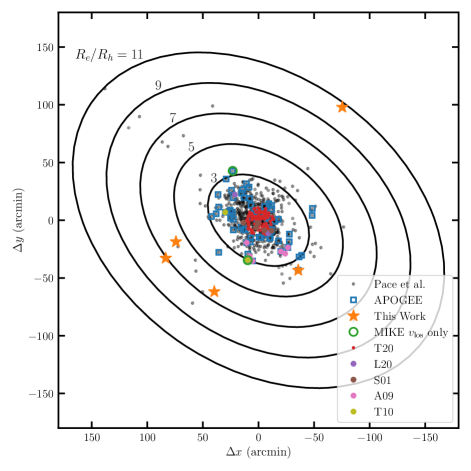
Figure 1: Plot of the spatial distribution of our sample (orange stars and green circles) and previous spectroscopic samples of stars in Sextans (catalog NAME SEXTANS DSPH): T20 = Theler et al. (2020), L20 = Lucchesi et al. (2020), S01 = Shetrone et al. (2001), A09 = Aoki et al. (2009), and T10 = Tafelmeyer et al. (2010). The small gray dots mark stars observed in our medium-resolution work (Pace et al., in preparation). The ellipses indicate multiples of $R_{\rm h}$.

Figure 2 illustrates the line-of-sight velocity, $v_{\rm los}$, as a function of radial distance from the center of the Sextans (catalog NAME SEXTANS DSPH) dSph. Our $v_{\rm los}$ measurements agree with previous values, when available, and they cluster around the systemic $v_{\rm los}$ of the Sextans (catalog NAME SEXTANS DSPH) dSph, $224.3\pm 0.1$ km s^-1 (Walker et al., 2009b). The stars in our sample are high-probability members of Sextans (catalog NAME SEXTANS DSPH).

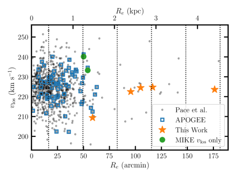
Figure 2: Comparison of $R_{\rm e}$ versus $v_{\rm los}$ for stars in Sextans (catalog NAME SEXTANS DSPH). The scale on the top axis assumes a distance of 86.1 kpc (Gaia Collaboration et al., 2018). Vertical dotted lines mark 1, 3, 5, 7 9, and 11 times $R_{\rm h}$. The five stars observed with high S/N in the present study are marked with orange stars, and the two stars observed with low S/N in the present study are marked with green circles. Previous samples from APOGEE (Abdurro’uf et al., 2022) and our own medium-resolution work (Pace et al., in preparation) are marked with open blue squares and small gray dots, respectively.

2.2 Observations

We used the Magellan Inamori Kyocera Echelle (MIKE; Bernstein et al. 2003) spectrograph on the Landon Clay (Magellan II) Telescope at Las Campanas Observatory, Chile, to collect high-resolution spectra of seven stars in Sextans (catalog NAME SEXTANS DSPH). These spectra were obtained on several nights in 2021 and 2022 during dark time and under excellent seeing conditions ($\approx 0\farcs 4$–0$\farcs$8). The 0$\farcs$7$\times$5$\farcs$0 entrance slit and 2$\times$2 binning on the CCD yield a spectral resolving power of $R\equiv\lambda/\Delta\lambda\sim 41,000$ on the blue spectrograph (3350 $<\lambda<$ 5000 Å) and $R\sim 36,000$ on the red spectrograph (5000 $<\lambda<$ 9150 Å). We observed each star using a series of exposures, ranging from 1500 s to 2300 s each. We obtained ThAr comparison spectra immediately before or after the series of exposures of each star. Table 2 summarizes the observing date, UT at mid observation, total exposure time, heliocentric $v_{\rm los}$, and S/N ratios at several wavelengths in the co-added spectrum of each star. We focus our attention on the five stars with high S/N ratios.

Table 2: Log of MIKE Observations

Star name	Obs. date	UT	$t_{\rm exp}$	$v_{\rm los}$	S/N@3950 Å	S/N@4550 Å	S/N@5200 Å	S/N@6700 Å
			(hr)	(km s-1)	(pix-1)	(pix-1)	(pix-1)	(pix-1)
Stars with high-S/N observations
J1008$+$0001	2022/03/03	04:42	5.56	$+$223.6	13	30	26	61
J1010$-$0220	2021/01/12	08:22	1.11	$+$209.0	17	34	30	67
	2021/01/13	04:58	2.56	$+$209.8
J1015$-$0238	2021/01/12	06:18	2.89	$+$224.5	15	31	28	64
J1018$-$0155	2021/01/13	07:34	2.47	$+$222.5	16	33	30	70
J1018$-$0209	2021/12/05	07:23	1.61	$+$224.7	13	30	27	66
	2021/12/06	07:24	1.67	$+$224.8
Stars with low-S/N observations
J1013$-$0211	2021/01/12	03:59	0.19	$+$242.1	3	8	8	19
J1014$-$0054	2021/01/12	04:27	0.19	$+$234.1	3	8	7	18

We use the CarPy MIKE reduction pipeline (Kelson et al., 2000; Kelson, 2003) to perform the overscan subtraction, pixel-to-pixel flat field division, image coaddition, cosmic ray removal, sky and scattered-light subtraction, rectification of the tilted slit profiles along the orders, spectrum extraction, and wavelength calibration. We use the IRAF (Tody, 1993) software package to stitch together and continuum-normalize the spectra.

Figure 3 illustrates several regions of the spectra around lines of interest. A few key features are immediately discernible. First, the differences in line strengths are mainly due to differences in abundance, because these stars have similar stellar parameters (Section 3.1). Secondly, lines of Ti and Fe exhibit only minimal differences, indicating that these stars have similar metallicities to within a factor of a few (Section 3.1). Thirdly, one star, J1008$+$0001, has much stronger CH, CN, [O i], Na i, Mg i, Si i, and K i lines, while its Ba ii and Eu ii lines are much weaker than those in other stars (Section 4.5). Finally, J1018$-$0155 (along with J1010$-$0220 and J1018$-$0209; not shown) exhibits moderately strong Eu ii lines, suggesting that these three stars are enhanced in r-process elements (Section 4.4).

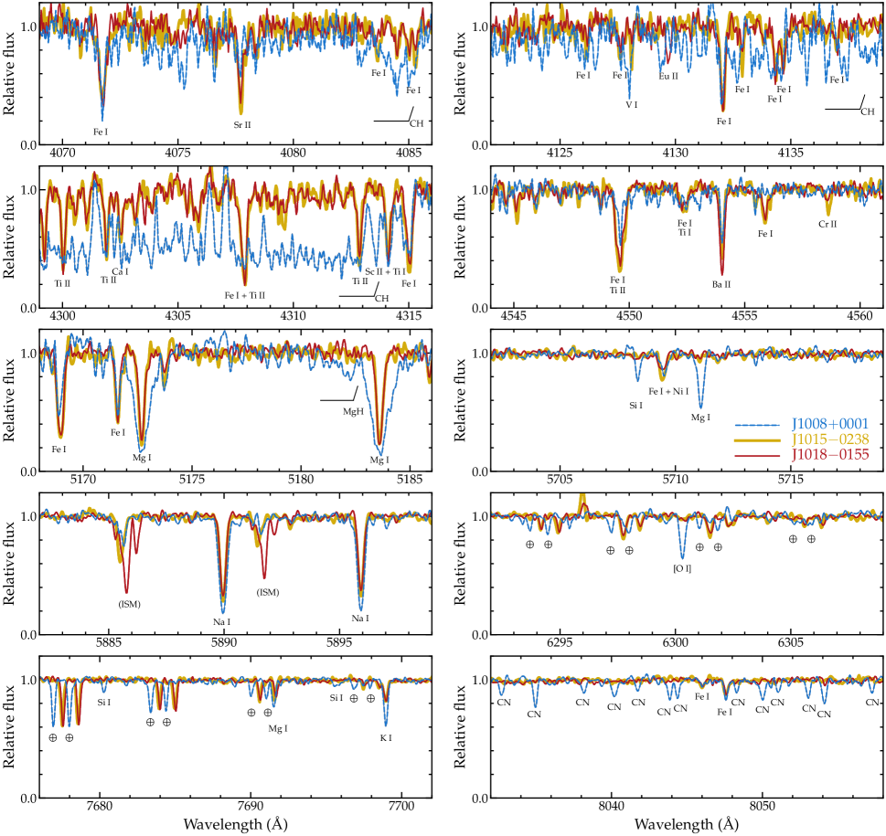
Figure 3: Selected regions of the MIKE spectra of three stars. Several absorption lines are identified. These three stars have similar $T_{\rm eff}$ and log g, so the differences in the line strengths mainly reflect abundance differences. Several interstellar medium (ISM) and O₂ telluric lines ($\earth$) are detected and marked. The telluric lines shift in velocity relative to the stellar lines, and they are marked at their approximate wavelengths in J1008$+$0001.

We measure $v_{\rm los}$ by cross-correlating the echelle order containing the Mg i b triplet against a metal-poor template spectrum obtained with MIKE, using the IRAF “fxcor” task. We calculate the heliocentric velocity corrections using the IRAF “rvcorrect” task. Roederer et al. (2014b) estimated uncertainties of $\approx 0.7$ km s^-1 for $v_{\rm los}$ values measured by this method. Repeat observations of J1010$-$0220 and J1018$-$0209 yield consistent $v_{\rm los}$ values that support this estimate.

3 Analysis

We describe our derivation of stellar parameters (Table 3) and abundances (Tables 4 through 7) in this section. We define the abundance of element X as $\log\varepsilon$(X) $\equiv\log_{10}(N_{\rm X}/N_{\rm H})+$12.0, where $N_{\rm X}$ represents the number density of element X. We define the abundance ratio of X and Fe relative to the solar ratio as [X/Fe] $\equiv\log_{10}(N_{\rm X}/N_{\rm Fe})-\log_{10}(N_{\rm X}/N_{\rm Fe})_{\odot}$. We adopt the solar abundances, listed in Table 5, from Asplund et al. (2009). By convention, abundances or ratios denoted with the ionization state (e.g., [Fe ii/H]) are understood to be the total elemental abundance as derived from transitions of that particular ionization state after Saha (1921) ionization corrections have been applied.

Table 3: Model Atmosphere Parameters

Star name	$T_{\rm eff}$	log g	$v_{\rm t}$	[M/H]	[Fe i/H]
	(K)		(km s-1)
J1008$+$0001	4405	1.07	2.25	$-$3.43	$-$2.97
J1010$-$0220	4405	0.79	2.15	$-$3.03	$-$3.34
J1015$-$0238	4441	0.79	2.35	$-$2.73	$-$2.64
J1018$-$0155	4423	0.72	2.45	$-$2.89	$-$2.81
J1018$-$0209	4396	0.67	2.45	$-$2.86	$-$2.75

3.1 Model Atmospheres

We derive model atmosphere parameters using a combination of quantities measured from the spectra themselves and values adopted from external catalogs. We interpolate models from the 1D ATLAS9 grid of $\alpha$-enhanced models (Castelli & Kurucz, 2004) using an interpolation code provided by A. McWilliam (2009, private communication).

We rely on abundances derived from equivalent widths (EWs) of Fe i and ii lines as part of this process. We measure EWs using a semi-automated routine that fits Voigt or Gaussian line profiles to continuum-normalized spectra (Roederer et al., 2014b). Each line is inspected visually. A telluric spectrum is simultaneously compared with the stellar spectrum, and we discard any lines that appear to be contaminated by telluric absorption. These Fe i and ii lines are listed in Table 4. We derive Fe abundances using a recent version of the line analysis software MOOG (Sneden 1973; Sobeck et al. 2011; 2017 version), which assumes local thermodynamic equilibrium (LTE).  We adopt damping constants for collisional broadening with neutral hydrogen from Barklem et al. (2000) and Barklem & Aspelund-Johansson (2005), when available, otherwise we adopt the standard Unsöld (1955) recipe. We discard strong Fe lines with $\log$(EW/$\lambda$) $>-4.5$. The weakest lines employed in our analysis have EW $\approx 7$ mÅ (Table 4).

Table 4: Line Atomic Data and Derived Abundances

						J1008$+$0001					J1010$-$0220				…
Species	$\lambda$	E.P.	$\log(gf)$	$\log(gf)$	$\log(gf)$	EW	U.L.	$\log\varepsilon$	NLTE		EW	U.L.	$\log\varepsilon$	NLTE	…
				unc.	ref.		flag	(LTE)	cor.			flag	(LTE)	cor.	…
	(Å)	(eV)				(mÅ)					(mÅ)				…
Li I	6707.80	0.00	0.17	0.01	1		$<$	0.10	+0.15			$<$	0.40	+0.15	…
O I	6300.30	0.00	$-$9.82	0.03	2	$\cdots$		8.07	$\cdots$		$\cdots$	$<$	6.70	$\cdots$	…
O I	6363.78	0.02	$-$10.26	0.03	2	$\cdots$		8.08	$\cdots$		$\cdots$		$\cdots$	$\cdots$	…
Na I	5682.63	2.10	$-$0.71	0.01	2	52.2		4.96	-0.13						…
Na I	5688.19	2.10	$-$0.41	0.01	2	69.9		4.91	-0.16						…
⋮	⋮	⋮	⋮	⋮	⋮	⋮	⋮	⋮	⋮		⋮	⋮	⋮	⋮	⋮

1: Smith et al. (1998), using HFS from Kurucz (2011); 2: Kramida et al. (2021); 3: Pehlivan Rhodin et al. (2017); 4: Kramida et al. (2021), using HFS from VALD3 (Piskunov et al., 1995; Pakhomov et al., 2019); 5: Den Hartog et al. (2023); 6: Den Hartog et al. (2021); 7: Lawler & Dakin (1989), using HFS from Kurucz (2011); 8: Lawler et al. (2013); 9: Pickering et al. (2001), using corrections given in Pickering et al. (2002); 10: Wood et al. (2013); 11: Lawler et al. (2014), including HFS; 12: Wood et al. (2014a), including HFS; 13: Sobeck et al. (2007); 14: Lawler et al. (2017); 15: Den Hartog et al. (2011), including HFS; 16: O’Brian et al. (1991); 17: Den Hartog et al. (2014); 18: Ruffoni et al. (2014); 19: Belmonte et al. (2017); 20: Blackwell et al. (1982); 21: Meléndez & Barbuy (2009); 22: Den Hartog et al. (2019); 23: Lawler et al. (2015), including HFS; 24: Wood et al. (2014b); 25: Roederer & Lawler (2012); 26: Biémont et al. (2011); 27: Ljung et al. (2006); 28: Kramida et al. (2021), using HFS/IS from McWilliam (1998) or other sources when available; 29: Lawler et al. (2001a), using HFS from Ivans et al. (2006) when available; 30: Lawler et al. (2009); 31: Li et al. (2007), using HFS from Sneden et al. (2009); 32: Den Hartog et al. (2003); 33: Lawler et al. (2006), using HFS/IS from Roederer et al. (2008); 34: Lawler et al. (2001b), using HFS/IS from Ivans et al. (2006); 35: Wickliffe et al. (2000); 36: Biémont et al. (2000), using HFS/IS from Roederer et al. (2012).

Note. — The complete version of Table 4 is available in machine-readable form in the online edition of the journal. A small section is shown here to illustrate its form and content.

Stellar effective temperatures ($T_{\rm eff}$) may be derived from photometric or spectroscopic methods. We derive $T_{\rm eff}$ values using the spectroscopic excitation balance method, and we apply a separate calibration (Frebel et al., 2013) to transform this scale, which is generally considered to be too cool, to the warmer photometric one. We begin by identifying the $T_{\rm eff}$, log of the surface gravity (log g; cm s^-2 in cgs units), microturbulent velocity parameter ($v_{\rm t}$), and model metallicity ([M/H]) that meet the following set of requirements. We set $T_{\rm eff}$ by requiring no trend between the abundance derived from Fe i lines and the lower excitation potential of each transition. We set $v_{\rm t}$ by requiring no trend between the abundance derived from Fe i lines and the line strength. We set log g by requiring that the mean abundances calculated from Fe i and ii lines agree within their uncertainties; in practice, these two quantities are closest at the edge of the model atmosphere grid at log g = 0.0. We set [M/H] by matching the Fe abundance (from Fe i lines) plus 0.25 dex as recommended by Frebel et al. Once these values converge, we calculate a corrected $T_{\rm eff}$ by extrapolating Equation 1 of Frebel et al. The corrected $T_{\rm eff}$ values are $\approx 250$ K warmer than the purely spectroscopic ones for these stars.

We use the corrected $T_{\rm eff}$ to calculate a new log g from fundamental relations:

$$\log g=4\log\mbox{$T_{\rm eff}$}+\log(M/\mbox{$M_{\odot}$})-10.61+0.4(BC_{V}$$

$$+m_{V}-5\log d+5-3.1E(B-V)-M_{\rm bol,\odot}).$$ (1)

Here, $M$ is the mass of the star, which we assume to be 0.8 $\pm$ 0.08 $M_{\odot}$. $BC_{V}$ is the bolometric correction in the $V$ band (Casagrande & VandenBerg, 2014). $m_{V}$ is the apparent $V$ magnitude. $d$ is the distance in pc, which is assumed to be 86.1 $\pm$ 2.6 kpc (Gaia Collaboration et al., 2018). We rederive $v_{\rm t}$ and metallicity and iterate on the stellar parameters, including $BC_{V}$, until the [M/H] matches [Fe ii/H] and there is no trend between the abundance derived from Fe i lines and the line strength.

Equation 3.1 requires an estimate of the reddening along the line of sight to each star, $E(B-V)$. We estimate $E(B-V)$ by two methods. We interpolate the dust maps presented by Schlafly & Finkbeiner (2011), which provide the $E(B-V)$ values along the line of sight, and we assume that all of the interstellar reddening lies in front of Sextans (catalog NAME SEXTANS DSPH). We also estimate $E(B-V)$ using the interstellar Na i D absorption (Bohlin et al., 1978; Spitzer, 1978; Ferlet et al., 1985), as described in Roederer et al. (2018b). We measure the EWs by direct integration using the IRAF “splot” task. For stars J1015$-$0238 and J1008$+$0001, the ratio of the EWs of the two components of the doublet is $\approx$2:1 (120:65 mÅ and 70:35 mÅ, respectively), the same as the ratio of the $f$-values of these transitions. These lines are on the linear part of the curve of growth and thus sensitive to the reddening. For the other three stars, multiple components are present, the EWs are larger, and they are not in 2:1 ratios (J1010$-$0220, 220:160 mÅ; J1018$-$0155, 345:235 mÅ; J1018$-$0209, 175:100 mÅ). They are saturated and so only yield limits on the amount of interstellar absorption. The empirical relations between Na i absorption, $N$(H i + H₂), and $E(B-V)$ have intrinsic scatter that corresponds to a few hundredths of a mag in $E(B-V)$. The two methods yield reasonably similar $E(B-V)$ values, which we list along with our adopted averages in Table 1. Our adopted set of stellar parameters is listed in Table 3.

We estimate the mean and uncertainty in each stellar parameter as follows. Frebel et al. (2013) estimate uncertainties in $T_{\rm eff}$ of $\approx 150$ K using their method. For log g, we draw $10^{4}$ samples from each input parameter in the log g calculation, assuming Gaussian uncertainties. The statistical uncertainty associated with this method is $\approx 0.09$ dex. The systematic uncertainty is certainly larger, $\sim 0.25$ dex or so (Jofré et al., 2019). For a given $T_{\rm eff}$ and log g, the uncertainty in $v_{\rm t}$ is $\approx 0.2$ km s^-1 and the uncertainty in [M/H] is $\approx 0.2$ dex.

The LTE [Fe/H] ratios derived from Fe i and Fe ii lines are not forced into agreement using this method. Non-LTE (NLTE) overionization of neutral Fe causes the Fe abundance from Fe i lines to be underestimated (Thévenin & Idiart, 1999). NLTE corrections for Fe ii lines are generally negligible. NLTE corrections are available for $\approx 25$ of the Fe i lines for which we have measured EWs. We evaluate these corrections by interpolating the pre-computed grids presented in the INSPECT database (Bergemann et al., 2012; Lind et al., 2012). The NLTE corrections range from $+$0.10 to $+$0.14 for these five stars. [Fe ii/Fe i] ionization equilibrium is achieved within 1.8$\sigma$ after including these NLTE corrections. We adopt the NLTE-corrected Fe abundance from Fe i lines when constructing abundance ratios of various elements relative to Fe (i.e., [X/Fe]).

Table 5: Derived Abundances (Part 1 of 3)

			J1008$+$0001						J1010$-$0220
Species	$Z$	$\log\varepsilon_{\odot}$	$\log\varepsilon$(X)	[X/Fe]	$\sigma$($\log\varepsilon$(X))	$\sigma$([X/Fe])	$N$		$\log\varepsilon$(X)	[X/Fe]	$\sigma$($\log\varepsilon$(X))	$\sigma$([X/Fe])	$N$
Li i	3	$\cdots$	$<$0.25	$\cdots$	$\cdots$	$\cdots$	1		$<$0.55	$\cdots$	$\cdots$	$\cdots$	1
C (CH)	6	8.43	7.41	$+$1.95	0.20	0.20	1		5.45	$+$0.36	0.20	0.20	1
N (CN)	7	7.83	6.70	$+$1.84	0.30	0.30	1		$\cdots$	$\cdots$	$\cdots$	$\cdots$	0
O i	8	8.69	8.08	$+$2.36	0.15	0.18	2		$<$6.70	$<+$1.35	$\cdots$	$\cdots$	1
Na i	11	6.24	4.86	$+$1.59	0.13	0.14	4		2.61	$-$0.29	0.29	0.11	2
Mg i	12	7.60	6.47	$+$1.84	0.21	0.13	3		4.47	$+$0.21	0.14	0.17	2
Al i	13	6.45	$<$5.20	$<+$1.72	$\cdots$	$\cdots$	2		3.07	$-$0.04	0.39	0.28	1
Si i	14	7.51	6.28	$+$1.74	0.10	0.18	13		4.27	$+$0.10	0.38	0.36	1
K i	19	5.03	3.34	$+$1.28	0.26	0.13	1		2.13	$+$0.44	0.22	0.13	2
Ca i	20	6.34	3.87	$+$0.50	0.16	0.09	14		3.15	$+$0.15	0.18	0.12	6
Sc ii	21	3.15	$-$0.23	$-$0.41	0.13	0.16	4		$-$0.30	$-$0.11	0.14	0.14	5
Ti i	22	4.95	2.40	$+$0.42	0.27	0.07	11		1.58	$-$0.03	0.31	0.13	5
Ti ii	22	4.95	1.81	$-$0.17	0.11	0.14	9		1.80	$+$0.19	0.11	0.10	16
V i	23	3.93	$\cdots$	$\cdots$	$\cdots$	$\cdots$	0		$\cdots$	$\cdots$	$\cdots$	$\cdots$	0
V ii	23	3.93	$\cdots$	$\cdots$	$\cdots$	$\cdots$	0		$\cdots$	$\cdots$	$\cdots$	$\cdots$	0
Cr i	24	5.64	2.64	$-$0.04	0.25	0.06	9		2.01	$-$0.29	0.27	0.12	4
Cr ii	24	5.64	$\cdots$	$\cdots$	$\cdots$	$\cdots$	0		2.40	$+$0.10	0.33	0.33	1
Mn i	25	5.43	2.46	$+$0.00	0.22	0.09	3		1.77	$-$0.32	0.28	0.20	1
Fe i	26	7.50	4.53	$-$2.97	0.22	0.22	70		4.16	$-$3.34	0.26	0.26	78
Fe ii	26	7.50	4.07	$-$3.43	0.14	0.14	2		4.47	$-$3.03	0.11	0.11	7
Co i	27	4.99	$\cdots$	$\cdots$	$\cdots$	$\cdots$	0		$\cdots$	$\cdots$	$\cdots$	$\cdots$	0
Ni i	28	6.22	3.40	$+$0.15	0.21	0.09	6		2.50	$-$0.38	0.25	0.10	1
Zn i	30	4.56	2.26	$+$0.67	0.10	0.23	2		1.67	$+$0.45	0.24	0.34	2
Sr ii	38	2.87	$-$2.47	$-$2.37	0.21	0.25	1		$-$0.97	$-$0.49	0.25	0.25	2
Y ii	39	2.21	$\cdots$	$\cdots$	$\cdots$	$\cdots$	0		$-$1.34	$-$0.21	0.19	0.19	3
Zr ii	40	2.58	$\cdots$	$\cdots$	$\cdots$	$\cdots$	0		$-$0.62	$+$0.15	0.26	0.28	2
Ba ii	56	2.18	$-$2.24	$-$1.45	0.17	0.20	3		$-$1.27	$-$0.10	0.16	0.16	4
La ii	57	1.10	$\cdots$	$\cdots$	$\cdots$	$\cdots$	0		$-$1.76	$+$0.49	0.22	0.22	2
Ce ii	58	1.58	$\cdots$	$\cdots$	$\cdots$	$\cdots$	0		$-$1.35	$+$0.42	0.50	0.50	2
Pr ii	59	0.72	$\cdots$	$\cdots$	$\cdots$	$\cdots$	0		$\cdots$	$\cdots$	$\cdots$	$\cdots$	0
Nd ii	60	1.42	$\cdots$	$\cdots$	$\cdots$	$\cdots$	0		$-$1.41	$+$0.51	0.25	0.26	2
Sm ii	62	0.96	$\cdots$	$\cdots$	$\cdots$	$\cdots$	0		$-$1.53	$+$0.86	0.50	0.50	2
Eu ii	63	0.52	$<-$2.40	$<+$0.05	$\cdots$	$\cdots$	2		$-$2.12	$+$0.70	0.20	0.21	3
Dy ii	66	1.10	$\cdots$	$\cdots$	$\cdots$	$\cdots$	0		$\cdots$	$\cdots$	$\cdots$	$\cdots$	0
Pb i	82	2.04	$<$0.60	$<+$1.53	$\cdots$	$\cdots$	1		$<$0.29	$<+$1.59	$\cdots$	$\cdots$	1

Note. — [Fe/H] is given instead of [X/Fe] for Fe. The C abundances have been corrected (by $+$0.41 and $+$0.75 dex) to the “natal” abundances according to the stellar evolution corrections presented by Placco et al. (2014). A single C abundance is derived by spectrum synthesis of the region from 4290–4330 Å.  NLTE corrections have been applied to the Li, Na, Mg, Al, Si, K, Fe i, and Pb abundances; see Table 4 for corrections and the text for references.

Table 6: Derived Abundances (Part 2 of 3)

			J1015$-$0238						J1018$-$0155
Species	$Z$	$\log\varepsilon_{\odot}$	$\log\varepsilon$(X)	[X/Fe]	$\sigma$($\log\varepsilon$(X))	$\sigma$([X/Fe])	$N$		$\log\varepsilon$(X)	[X/Fe]	$\sigma$($\log\varepsilon$(X))	$\sigma$([X/Fe])	$N$
Li i	3	$\cdots$	$<$0.21	$\cdots$	$\cdots$	$\cdots$	1		$<$0.51	$\cdots$	$\cdots$	$\cdots$	1
C (CH)	6	8.43	5.77	$-$0.22	0.20	0.20	1		5.37	$-$0.25	0.20	0.20	1
N (CN)	7	7.83	$\cdots$	$\cdots$	$\cdots$	$\cdots$	0		$\cdots$	$\cdots$	$\cdots$	$\cdots$	0
O i	8	8.69	$<$6.70	$<+$0.65	$\cdots$	$\cdots$	1		$<$6.80	$<+$0.92	$\cdots$	$\cdots$	1
Na i	11	6.24	3.62	$+$0.02	0.38	0.16	2		3.50	$+$0.07	0.35	0.15	2
Mg i	12	7.60	5.19	$+$0.23	0.18	0.17	3		5.11	$+$0.32	0.14	0.14	2
Al i	13	6.45	3.92	$+$0.11	0.39	0.25	1		4.38	$+$0.74	0.38	0.24	1
Si i	14	7.51	5.07	$+$0.20	0.43	0.37	1		4.71	$+$0.01	0.40	0.36	1
K i	19	5.03	2.42	$+$0.03	0.21	0.07	2		2.40	$+$0.18	0.20	0.07	2
Ca i	20	6.34	3.82	$+$0.12	0.17	0.09	15		3.65	$+$0.12	0.16	0.10	12
Sc ii	21	3.15	0.31	$-$0.20	0.11	0.11	9		0.17	$-$0.17	0.11	0.10	9
Ti i	22	4.95	2.35	$+$0.04	0.29	0.07	16		2.08	$-$0.06	0.29	0.09	10
Ti ii	22	4.95	2.58	$+$0.27	0.11	0.09	25		2.27	$+$0.13	0.09	0.09	20
V i	23	3.93	0.94	$-$0.35	0.31	0.11	3		0.87	$-$0.25	0.32	0.16	3
V ii	23	3.93	1.22	$-$0.07	0.17	0.17	2		1.05	$-$0.07	0.30	0.29	1
Cr i	24	5.64	2.77	$-$0.23	0.27	0.07	7		2.45	$-$0.38	0.25	0.06	8
Cr ii	24	5.64	3.07	$+$0.07	0.15	0.12	2		2.67	$-$0.16	0.28	0.27	1
Mn i	25	5.43	2.38	$-$0.41	0.23	0.09	3		2.08	$-$0.54	0.22	0.10	3
Fe i	26	7.50	4.86	$-$2.64	0.24	0.24	115		4.69	$-$2.81	0.24	0.24	107
Fe ii	26	7.50	4.77	$-$2.73	0.11	0.11	10		4.61	$-$2.89	0.11	0.11	11
Co i	27	4.99	2.06	$-$0.29	0.34	0.16	1		1.84	$-$0.34	0.31	0.14	1
Ni i	28	6.22	3.56	$-$0.02	0.21	0.08	6		3.30	$-$0.11	0.23	0.13	5
Zn i	30	4.56	2.24	$+$0.32	0.11	0.24	2		1.83	$+$0.08	0.17	0.27	2
Sr ii	38	2.87	0.31	$+$0.08	0.18	0.19	2		$-$0.72	$-$0.78	0.25	0.25	2
Y ii	39	2.21	$-$0.80	$-$0.37	0.12	0.13	3		$-$1.39	$-$0.79	0.16	0.17	2
Zr ii	40	2.58	0.01	$+$0.07	0.15	0.15	3		$-$0.52	$-$0.29	0.21	0.21	3
Ba ii	56	2.18	$-$1.59	$-$1.13	0.15	0.16	4		$-$0.94	$-$0.31	0.15	0.15	4
La ii	57	1.10	$\cdots$	$\cdots$	$\cdots$	$\cdots$	0		$-$1.71	$+$0.00	0.23	0.24	5
Ce ii	58	1.58	$\cdots$	$\cdots$	$\cdots$	$\cdots$	0		$-$1.20	$+$0.03	0.26	0.27	2
Pr ii	59	0.72	$\cdots$	$\cdots$	$\cdots$	$\cdots$	0		$-$1.62	$+$0.47	0.27	0.28	1
Nd ii	60	1.42	$\cdots$	$\cdots$	$\cdots$	$\cdots$	0		$-$1.15	$+$0.24	0.20	0.20	3
Sm ii	62	0.96	$\cdots$	$\cdots$	$\cdots$	$\cdots$	0		$-$1.73	$+$0.12	0.45	0.45	1
Eu ii	63	0.52	$<-$2.70	$<-$0.58	$\cdots$	$\cdots$	2		$-$1.96	$+$0.33	0.15	0.15	3
Dy ii	66	1.10	$\cdots$	$\cdots$	$\cdots$	$\cdots$	0		$-$1.06	$+$0.65	0.43	0.44	1
Pb i	82	2.04	$<$0.10	$<+$0.70	$\cdots$	$\cdots$	1		$<$0.05	$<+$0.82	$\cdots$	$\cdots$	1

Note. — [Fe/H] is given instead of [X/Fe] for Fe. The C abundances have been corrected (by $+$0.77 and $+$0.76 dex) to the “natal” abundances according to the stellar evolution corrections presented by Placco et al. (2014). A single C abundance is derived by spectrum synthesis of the region from 4290–4330 Å.  NLTE corrections have been applied to the Li, Na, Mg, Al, Si, K, Fe i, and Pb abundances; see Table 4 for corrections and the text for references.

Table 7: Derived Abundances (Part 3 of 3)

			J1018$-$0209
Species	$Z$	$\log\varepsilon_{\odot}$	$\log\varepsilon$(X)	[X/Fe]	$\sigma$($\log\varepsilon$(X))	$\sigma$([X/Fe])	$N$
Li i	3	$\cdots$	$<$0.25	$\cdots$	$\cdots$	$\cdots$	1
C (CH)	6	8.43	5.34	$-$0.34	0.20	0.20	1
N (CN)	7	7.83	$\cdots$	$\cdots$	$\cdots$	$\cdots$	0
O i	8	8.69	$<$6.90	$<+$0.96	$\cdots$	$\cdots$	1
Na i	11	6.24	3.25	$-$0.24	0.24	0.08	3
Mg i	12	7.60	5.15	$+$0.30	0.15	0.13	5
Al i	13	6.45	3.30	$-$0.40	0.40	0.28	1
Si i	14	7.51	4.98	$+$0.22	0.26	0.26	2
K i	19	5.03	2.36	$+$0.08	0.21	0.09	1
Ca i	20	6.34	3.63	$+$0.04	0.16	0.10	13
Sc ii	21	3.15	0.08	$-$0.32	0.11	0.11	8
Ti i	22	4.95	2.05	$-$0.15	0.30	0.07	11
Ti ii	22	4.95	2.19	$-$0.01	0.10	0.09	20
V i	23	3.93	0.60	$-$0.58	0.34	0.19	1
V ii	23	3.93	1.18	$+$0.00	0.23	0.23	2
Cr i	24	5.64	2.53	$-$0.36	0.27	0.06	5
Cr ii	24	5.64	$\cdots$	$\cdots$	$\cdots$	$\cdots$	0
Mn i	25	5.43	2.07	$-$0.61	0.22	0.09	3
Fe i	26	7.50	4.75	$-$2.75	0.25	0.25	113
Fe ii	26	7.50	4.64	$-$2.86	0.10	0.10	13
Co i	27	4.99	$\cdots$	$\cdots$	$\cdots$	$\cdots$	0
Ni i	28	6.22	3.32	$-$0.15	0.23	0.07	4
Zn i	30	4.56	2.00	$+$0.19	0.12	0.26	2
Sr ii	38	2.87	$-$0.73	$-$0.85	0.25	0.23	2
Y ii	39	2.21	$-$1.21	$-$0.67	0.14	0.15	3
Zr ii	40	2.58	$-$0.58	$-$0.41	0.23	0.24	1
Ba ii	56	2.18	$-$0.87	$-$0.30	0.18	0.17	5
La ii	57	1.10	$-$1.77	$-$0.12	0.19	0.20	2
Ce ii	58	1.58	$-$1.37	$-$0.20	0.50	0.50	2
Pr ii	59	0.72	$\cdots$	$\cdots$	$\cdots$	$\cdots$	0
Nd ii	60	1.42	$\cdots$	$\cdots$	$\cdots$	$\cdots$	0
Sm ii	62	0.96	$-$1.64	$+$0.15	0.50	0.50	2
Eu ii	63	0.52	$-$2.06	$+$0.17	0.20	0.21	3
Dy ii	66	1.10	$\cdots$	$\cdots$	$\cdots$	$\cdots$	0
Pb i	82	2.04	$<$0.00	$<+$0.71	$\cdots$	$\cdots$	1

Note. — [Fe/H] is given instead of [X/Fe] for Fe. The C abundance has been corrected (by $+$0.77 dex) to the “natal” abundance according to the stellar evolution corrections presented by Placco et al. (2014). A single C abundance is derived by spectrum synthesis of the region from 4290–4330 Å.  NLTE corrections have been applied to the Li, Na, Mg, Al, Si, K, Fe i, and Pb abundances; see Table 4 for corrections and the text for references.

3.2 Abundance Derivations

We use the MOOG “abfind” driver to derive abundances from EWs of Mg i, Ca i, Ti i and ii, Cr i and ii, Fe i and ii, Ni i, and some Zn i lines. Lines of these species are unblended, are comprised of a single or dominant isotope or do not exhibit any significant line broadening by isotope shifts (IS), and do not exhibit any significant line broadening by hyperfine structure (HFS). All other abundances are derived by matching synthetic spectra generated using the MOOG “synth” driver to the observed spectrum. We produce line lists for these synthetic spectra using the LINEMAKE code (Placco et al., 2021a). We assume ¹²C/¹³C = 4, all N is ¹⁴N, and r-process isotopic ratios (Sneden et al., 2008) in our syntheses. Upper limits (U.L.) are reported for a few key species based on the non-detection of one or more lines in our spectra. Table 4 reports the wavelengths ($\lambda$), excitation potentials (E.P.), $\log(gf)$ values and their references, along with the EWs and LTE abundances for each line in each star.

We apply NLTE corrections, when available and potentially non-negligible, to the LTE abundances of each line of Li i (Lind et al., 2009), Na i (Lind et al., 2011), Mg i (Osorio et al., 2015; Osorio & Barklem, 2016), Al i (Nordlander & Lind, 2017), Si i (Shi et al., 2009), K i (Takeda et al., 2002), and Pb i (Mashonkina et al., 2012). The Li i, Na i, and Mg i NLTE corrections are accessed through the INSPECT database. The stellar parameters occasionally lie beyond the edge of pre-computed grids (usually in $T_{\rm eff}$ or log g, with edges at 4500 K or 1.0 dex, respectively), and in these cases we adopt the correction at the nearest point on the grid. Table 4 lists the line-by-line NLTE corrections, and Tables 5–7 list the NLTE-corrected mean abundances.

We compute abundance uncertainties by drawing $10^{3}$ resamples of the model atmosphere parameters, $\log(gf)$ values, and EWs (or approximations to the EWs for lines whose abundance was derived using spectrum synthesis), assuming Gaussian uncertainties. The uncertainties on the model atmosphere parameters are discussed in Section 3.1. The uncertainties in the $\log(gf)$ values are taken from the grades assigned by the National Institutes of Standards and Technology (NIST) Atomic Spectra Database (ASD, version 5.9; Kramida et al. 2021) or the original source references listed in Table 4. We assume a 5% uncertainty in the EWs, or a 5 mÅ minimum uncertainty in the case of weak lines, which accounts for continuum placement and unidentified weak blends. We also include a wavelength-dependent component of EW uncertainty that reflects the low S/N at blue wavelengths, which we empirically determine to be $\sigma_{\rm EW}=10^{24}\lambda^{-6.4}$, where the wavelength, $\lambda$, is measured in Å and $\sigma_{\rm EW}$ is measured in mÅ.  This component of the uncertainty is $\approx 9$ mÅ at 4000 Å, $\approx 4$ mÅ at 4500 Å, $\approx 2$ mÅ at 5000 Å, and $<$ 1 mÅ at 6000 Å. The mean abundance of each element is recomputed for each resample, and the final abundance uncertainties reported in Tables 5–7 represent the 16th and 84th percentiles (i.e., 1$\sigma$ range) of the distributions, which are roughly symmetric in most cases.

The uncertainties are generally smallest when the abundance is derived from several lines with $\lambda\gtrsim$ 4500 Å, where the S/N is highest. There are several heavy elements, including Ce, Pr, Sm, and Dy, whose abundances are derived from a small number (1 or 2) of very weak (EW $<$ 10 mÅ or so) lines in the blue part of the spectrum ($\lambda<$ 4500 Å).  The abundances are in agreement when multiple lines of one of these elements are detected in a star, which boosts our confidence in the legitimacy of their detection despite the relatively large uncertainties.

4 Results

In this section we present our abundance results and compare with previous work. Our sample contains no stars in common with previous high-resolution abundance studies. Figure 4 shows the abundance ratios for the stars in our sample, previous results for Sextans (catalog NAME SEXTANS DSPH) stars, and metal-poor field stars in the solar neighborhood. Several studies have reobserved or reanalyzed spectra of Sextans (catalog NAME SEXTANS DSPH) stars. We display these results in Figure 4 with lines connecting the different results for individual stars.

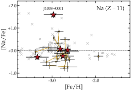
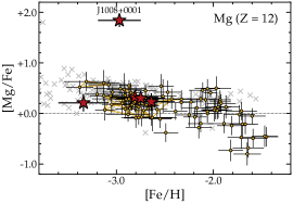
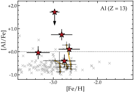
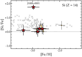
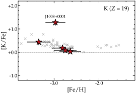
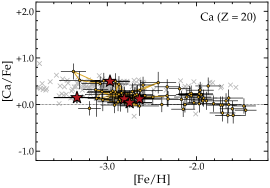
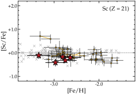
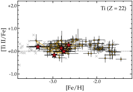
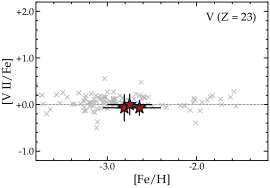
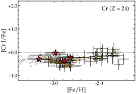
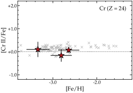
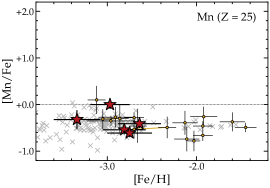
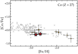
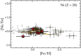
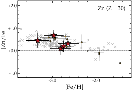
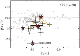
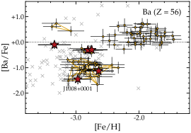
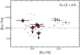
Figure 4: Abundance ratios for stars in our sample (large red stars) compared with previous results for Sextans (catalog NAME SEXTANS DSPH) stars (yellow circles) and metal-poor field stars (gray crosses). Yellow lines connect stars reobserved or reanalyzed by previous studies. The Sextans (catalog NAME SEXTANS DSPH) sample includes results from Shetrone et al. (2001), Aoki et al. (2009), Tafelmeyer et al. (2010), Honda et al. (2011), Mashonkina et al. (2017, 2022), Aoki et al. (2020), and Lucchesi et al. (2020). The field sample includes red giants ($T_{\rm eff}$ $<$ 5400 K) from Cayrel et al. (2004), Lai et al. (2008), Yong et al. (2013), Roederer et al. (2014b), and Ou et al. (2020). Abundances in the comparison samples have been computed in LTE, except for Na in most studies, and most abundances in the 11 stars studied by Mashonkina et al. (2017, 2022). The panels are arranged in order of increasing atomic number ($Z$).

4.1 $\alpha$ Elements: O, Mg, Si, Ca, and Ti

We detect five $\alpha$ elements in our sample: O ($Z=8$), Mg ($Z=12$), Si ($Z=14$), Ca ($Z=20$), and Ti ($Z=22$). We detect O only in J1008$+$0001, which we discuss separately in Section 4.5. The mean [Mg/Fe], [Si/Fe], [Ca/Fe], and [Ti/Fe] ratios found in the other four stars in our sample, weighted by their inverse-squared uncertainties, are $+0.27\pm 0.08$, $+0.15\pm 0.16$, $+0.10\pm 0.05$, and $+0.14\pm 0.05$, respectively. The weighted mean [$\alpha$/Fe] ratio in these four stars is $+0.12\pm 0.03$. As shown in Figure 4, these ratios are enhanced relative to the solar ratios, but they are a few tenths of a dex low relative to the mean ratios in field red giants with similar low metallicities. These [$\alpha$/Fe] ratios could indicate a deficiency of metals produced by the highest-mass stars (e.g., McWilliam et al. 2013).

Our result is broadly consistent with abundances derived previously from high-resolution spectra of the most metal-poor Sextans (catalog NAME SEXTANS DSPH) stars known (Shetrone et al., 2001; Aoki et al., 2009; Tafelmeyer et al., 2010; Aoki et al., 2020; Mashonkina et al., 2022). Our mean [Mg/Fe] abundance is in agreement with that derived by Mashonkina et al. from their homogeneous NLTE reanalysis of 10 Sextans (catalog NAME SEXTANS DSPH) stars with $-3.2\leq$ [Fe/H] $\leq-2.6$, [Mg/Fe] = $+0.27\pm 0.08$; our value is also in agreement with their LTE value, [Mg/Fe] = $+0.24\pm 0.08$. Our mean [Ca/Fe] abundance is lower than than the NLTE derived by Mashonkina et al., [Ca/Fe] = $+0.31\pm 0.06$, but it is in agreement with their LTE value, [Ca/Fe] = $+0.16\pm 0.06$.

Previous studies generally agree that there is a decline in the [$\alpha$/Fe] ratios at higher metallicities. There is mild disagreement about the placement of the knee in the [$\alpha$/Fe] versus [Fe/H] relation. Reichert et al. (2020) found a hint that there may be two knees in the [Mg/Fe] versus [Fe/H] relation, at [Fe/H] $=-2.5$ and $-2.0$, which could be a consequence of the accretion history of Sextans (catalog NAME SEXTANS DSPH). Mashonkina et al. (2022) discuss this issue in more detail. Our sample only includes stars with [Fe/H] $<-2.6$, so we are unable to contribute to this particular debate.

4.2 Other Light Elements: Li, C, N, Na, Al, K

Li ($Z=3$) is not detected in any star in our sample. The upper limits on the Li abundances, $\log\varepsilon$(Li) $<0.6$, are lower than the traditional Spite & Spite (1982) Plateau value, $\log\varepsilon$(Li) $\approx 2.2$, and the slight downturn in Li abundances found in unevolved stars with [Fe/H] $<-2.8$ (Sbordone et al., 2010). The low Li abundances in our stars are consistent with the well-established phenomenon wherein Li in the atmospheres is diluted as the base of the convective zone deepens to hotter layers during normal stellar evolution up the red giant branch.

C ($Z=6$) is detected in all five stars in our sample via the CH A-X (G) band. We derive the C abundance in each star by synthesizing the CH features in the 4290–4330 Å wavelength region, using lines from Masseron et al. (2014). The C abundances have been corrected to account for CN processing during normal stellar evolution (Placco et al., 2014), so the values presented in Tables 5–7 reflect the natal C abundances. The corrections for four of the stars are $\approx+0.75$ dex, and their corrected [C/Fe] ratios are solar to within a factor of $\approx 2$. Only one of the five stars, J1008$+$0001, is C enhanced. Its evolutionary correction is $+$0.41 dex, yielding a natal [C/Fe] = $+1.95\pm 0.20$. We discuss this carbon-enhanced metal-poor (CEMP) star in Section 4.5.

N ($Z=7$) is detected only in the CEMP star in our sample via the CN A-X (red system) bands. We derive the N abundance from the CN features in the 8000–8100 Å wavelength region, using lines from Sneden et al. (2014). The natal N abundance in this star is difficult to infer, because a wide range of initial—lower—N abundances can yield similar surface N abundances as CN-processed and N-enhanced material is dredged up during stellar evolution (Placco et al., 2014). We adopt the current surface abundance, [N/Fe] $=+1.84\pm 0.30$, as the natal abundance, but we recommend that it be interpreted with caution.

Na ($Z=11$) is detected in all five stars in our sample. The NLTE-corrected [Na/Fe] ratios are solar to within a factor of $\approx 2$ in four of the five stars. They fall within the range of metal-poor field stars and previously examined stars in the inner region of Sextans (catalog NAME SEXTANS DSPH). The [Na/Fe] ratio is highly enhanced, [Na/Fe] = $+1.59\pm 0.14$, in the CEMP star.

Al ($Z=13$) is detected in all five stars. We apply NLTE corrections to the LTE abundances in Tables 5–7. Figure 4, however, only shows the LTE abundances for the sake of comparing with literature data, which generally have not been corrected for NLTE.  The [Al/Fe] ratios are within the range of field stars and other Sextans (catalog NAME SEXTANS DSPH) stars. Two of the stars in our sample exhibit solar [Al/Fe] ratios in NLTE, which is common among stars with [Fe/H] $<-2$ (e.g., Andrievsky et al. 2008; Roederer & Lawler 2021). One star, J1018$-$0155, exhibits significantly enhanced [Al/Fe] = $+0.74\pm 0.24$ in NLTE.  Another star, J1018$-$0209, is moderately deficient in Al, with [Al/Fe] = $-0.40\pm 0.28$. No other abundance anomalies are found among light elements in either of these two stars, and we lack a satisfactory explanation for the differences in their Al abundances. There is no reliable Al abundance indicator in our spectrum of the CEMP star. The lines of the resonance Al i doublet at 3944 and 3961 Å are detected but heavily blended with CH features. The high-excitation Al i doublet at 6696 and 6698 Å is weak and undetected in our spectrum. We derive an upper limit on the Al abundance in this star, [Al/Fe] $<+1.72$, using the latter doublet.

K ($Z=19$) is detected in all five stars. K has not been detected previously in any star in Sextans (catalog NAME SEXTANS DSPH). The mean NLTE [K/Fe] ratio in the four non-CEMP stars, $+0.10\pm 0.04$, falls within the same range as the mean [$\alpha$/Fe] ratios in these stars. These [K/Fe] ratios also overlap with those of halo stars at similar metallicities. The CEMP star exhibits highly enhanced K, [K/Fe] = $+1.28\pm 0.13$. This value is higher than that for any star listed in the JINABase abundance database (Abohalima & Frebel, 2018).

4.3 Iron-Group Elements: Sc–Zn

Several iron-group elements, including Ti ($Z=22$), V ($Z=23$), and Cr ($Z=24$), are detected in multiple ionization states. The differences in the abundances derived from these different states are generally consistent from one star to another: $\approx+0.2$ dex for Ti (with the exception of J1008$+$0001), $\approx+0.3$ dex for V, and $\approx+0.3$ dex for Cr. The ions yield higher abundances than the neutrals. These differences are broadly consistent with previous NLTE calculations that suggest the differences in Ti and Cr can be attributed to NLTE overionization of the minority neutral species in cool, metal-poor giants (e.g., Bergemann & Cescutti 2010; Sitnova et al. 2016). Similar NLTE calculations for V have not been made. The ions should yield more reliable abundances of these species.

The mean [X/Fe] ratios of most iron-group elements are within $\approx 0.2$ dex of the solar ratios: [Sc/Fe] $=-0.21\pm 0.06$, [Ti/Fe] $=+0.14\pm 0.05$, [V/Fe] $=-0.04\pm 0.16$, [Cr/Fe] $=-0.02\pm 0.12$, and [Ni/Fe] $=-0.15\pm 0.04$. The mean [Mn/Fe] and [Co/Fe] ratios are deficient relative to the solar ratios, $-0.31\pm 0.05$ and $-0.33\pm 0.13$, respectively. Both Mn and Co are detected only in their neutral states, which could underestimate their abundances by several tenths of a dex (e.g., Bergemann & Gehren 2008; Bergemann et al. 2010). The mean [Zn/Fe] ratio is enhanced relative to the solar ratio, $+0.30\pm 0.13$. As shown in Figure 4, all of these ratios overlap with the range of ratios in stars in the inner region of Sextans (catalog NAME SEXTANS DSPH) and metal-poor field stars.

Cowan et al. (2020) and Sneden et al. (2023) have shown that the [Sc/Fe], [Ti/Fe], and [V/Fe] ratios are correlated in metal-poor field stars. The mean [Sc/Fe], [Ti/Fe], and [V/Fe] ratios in our Sextans (catalog NAME SEXTANS DSPH) stars are lower by $\approx$0.1–0.2 dex than the means in the metal-poor field star samples. These three ratios in our Sextans (catalog NAME SEXTANS DSPH) stars match the low end of the correlations found by Sneden et al., as shown in their Figure 7. This finding suggests that the supernovae that produced the bulk of the $\alpha$ and iron-group elements in our Sextans (catalog NAME SEXTANS DSPH) stars were not atypical, yet they produced slight deficiencies in most elements relative to Fe. We encourage new theoretical investigations of supernova yields to better understand this behavior.

4.4 Heavy Elements: Sr–Pb

We detect Sr ($Z=38$) and Ba ($Z=56$) in all stars in our sample, and elements heavier than Ba can be detected in three of the five stars. As shown in Figure 4, four of the five [Sr/Fe] ratios are comparable to those found in Sextans (catalog NAME SEXTANS DSPH) stars examined previously, $-0.85\leq$ [Sr/Fe] $\leq+0.08$. In contrast, the [Sr/Fe] ratio in the CEMP star, $-2.37\pm 0.25$, is $\approx$1 dex lower than any other star known in Sextans (catalog NAME SEXTANS DSPH). The [Ba/Fe] ratios in three of the stars, $-0.31\leq$ [Ba/Fe] $\leq-0.10$, are higher than most other Sextans (catalog NAME SEXTANS DSPH) stars with [Fe/H] $<-2.6$. The two other stars, including the CEMP star, exhibit [Ba/Fe] ratios nearly one dex lower.

Figure 5 illustrates the heavy-element abundance pattern in the five Sextans (catalog NAME SEXTANS DSPH) stars. The solar system r-process and s-process abundance patterns, normalized to the Ba abundance in each star, are shown for comparison (Prantzos et al., 2020). The s-process pattern is disfavored. Furthermore, enhanced Pb ($Z=82$) abundances are also signatures of s-process enrichment in metal-poor stars (Roederer et al., 2010a), and we do not detect an enhanced Pb abundance in any star in our sample.

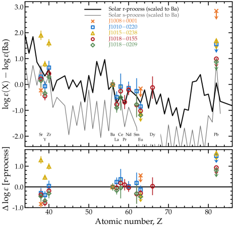
Figure 5: Heavy-element abundance patterns in the five Sextans (catalog NAME SEXTANS DSPH) stars. The top panel illustrates the abundance patterns, which have been normalized to $\log\varepsilon$(Ba) = 0.0. The bold black line marks the scaled solar r-process pattern, and the thin gray line marks the scaled solar s-process pattern (Prantzos et al., 2020). The Pb and Bi abundances in the s-process pattern have been enhanced by $+1.0$ dex relative to the solar pattern to account for the effect of low-metallicity AGB stars (cf. Figure 20 of Sneden et al. 2008, as calculated in the Appendix of Roederer et al. 2010b). The bottom panel illustrates the differences between the observed abundance patterns and the scaled solar r-process pattern.

The abundance patterns in J1010$-$0220, J1018$-$0155, and J1018$-$0209 are a reasonably close match to the solar r-process pattern. The most discrepant element, Y ($Z=39$), is only discrepant because the solar r-process pattern overestimates Y by $\approx$0.5 dex (e.g., Roederer et al. 2018a). Otherwise, all 11 detected heavy elements lie within 2$\sigma$ of the r-process pattern in these three stars. Furthermore, the [Ba/Eu] ratio, which is an indicator of the ratio of r-process to s-process material in a star, is low in these three stars ($-0.80$, $-0.64$, and $-0.47$). Material where the r-process is dominant will exhibit [Ba/Eu] $\approx-0.7\pm 0.2$ (e.g., Sneden et al. 2008; Mashonkina & Christlieb 2014; Prantzos et al. 2020; Roederer et al. 2023), whereas material where the s-process is dominant will exhibit [Ba/Eu] $>+1$ (e.g., Sneden et al. 2008; Bisterzo et al. 2014). We conclude that the main component of the r-process is the dominant source of the heavy elements in J1010$-$0220, J1018$-$0155, and J1018$-$0209.

Eu ($Z=63$) is frequently chosen to represent the level of r-process enhancement in stars. J1010$-$0220, J1018$-$0155, and J1018$-$0209 are enhanced in r-process elements, [Eu/Fe] = $+0.70\pm 0.21$, $+0.33\pm 0.15$, and $+0.17\pm 0.21$, respectively. J1010$-$0220 and J1018$-$0155 are therefore members of the r-I class of moderately r-process-enhanced stars, as defined by Beers & Christlieb (2005) and revised by Holmbeck et al. (2020). This level of enhancement is not as extreme as found in the r-process-enhanced UFD galaxy Reticulum II (catalog NAME RETICULUM II) ($+1.0<$ [Eu/Fe] $<+2.1$; Ji et al. 2016; Roederer et al. 2016), but it is similar to that in the moderately r-process-enhanced UFD galaxy Tucana III (catalog NAME TUCANA III) ($+0.2<$ [Eu/Fe] $<+0.6$; Hansen et al. 2017; Marshall et al. 2019). Stars with comparable [Eu/Fe] ratios are found in the Carina (catalog NAME CARINA DSPH), Draco (catalog NAME DRACO DSPH), and Ursa Minor (catalog NAME UMI DSPH) dSph galaxies, although only at higher metallicities ([Fe/H] $>-2.5$; Shetrone et al. 2003; Cohen & Huang 2009, 2010; Venn et al. 2012; Norris et al. 2017).

The other two stars in our sample, J1008$+$0001 and J1015$-$0238, exhibit different heavy-element abundance patterns. We discuss J1008$+$0001 separately in Section 4.5. J1015$-$0238 has more Sr and less Ba than the other stars in our sample: $\log\varepsilon$(Sr/Ba) $=1.90\pm 0.23$ ([Sr/Ba] $=+1.21\pm 0.25$), whereas $\log\varepsilon$(Sr/Ba) $\approx 0.21\pm 0.18$ ([Sr/Ba] $=-0.48\pm 0.18$) for the three r-process-enhanced stars. The weak component of the r-process (e.g., Wanajo 2013) and the weak component of the s-process (e.g., Frischknecht et al. 2016) are predicted to be capable of producing enhanced Sr/Ba ratios, and either process could be responsible for the heavy elements in J1015$-$0238. These processes are associated with core-collapse supernovae or their progenitor stars.

4.5 J1008+0001: a CEMP-no Star in Sextans

The star J1008$+$0001 is located at a projected radius of 10.7 $R_{\rm h}$ (4.3 kpc) from the center of Sextans (catalog NAME SEXTANS DSPH), and it is the most widely separated confirmed member of Sextans (catalog NAME SEXTANS DSPH) at present. It is highly enhanced ([X/Fe] $>+1.2$) in the light elements X = C, N, O, Na, Mg, Si, and K. Its [Ca/Fe] ratio, $+0.50\pm 0.09$, is higher than that found in the other four stars in our sample, $+0.10\pm 0.05$. It is also highly deficient ([X/Fe] $<-1.4$) in the heavy elements X = Sr and Ba. These characteristics identify J1008$+$0001 as a member of the class of carbon-enhanced metal-poor stars with no enhancement of neutron-capture elements (CEMP-no; Beers & Christlieb 2005). Such stars are thought to be among the first Population II stars to have formed and among the oldest surviving stars (Norris et al., 2013). No CEMP-no stars have been identified previously in Sextans (catalog NAME SEXTANS DSPH).

There have been two measurements of $v_{\rm los}$ of this star. One is our measurement ($+223.6\pm 0.7$ km s^-1; Table 2), and the other is an unpublished GIRAFFE measurement obtained on 2019 March 12 as part of a separate program ($+224.4\pm 5$ km s^-1; S. Koposov et al., in preparation). This star does not exhibit any discernible velocity variations over a span of 3 years, tentatively suggesting it is not part of a binary or multiple star system.

We fit the light-element abundance pattern (C through Zn; 6 $\leq Z\leq$ 30) of J1008$+$0001 using the yields predicted for zero-metallicity Population III supernovae. We consider theoretical nucleosynthesis yields from the grid of 1D supernova models of Heger & Woosley (2010), which includes non-rotating stars with initial masses ranging from 10 to 100 $M_{\odot}$, explosion energies ranging from $0.3\times 10^{51}$ to $10\times 10^{51}$ erg, and various degrees of mixing among the ejecta. We construct $10^{5}$ representations of the observed abundance pattern by resampling the $\log\varepsilon$ abundances from Gaussian distributions with standard deviations given by the observational uncertainties. We find the best-fit model for each resampled abundance pattern using a $\chi^{2}$ matching algorithm, as described in Placco et al. (2015, 2021b).

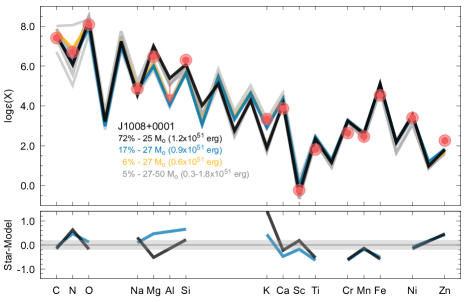
Figure 6: Comparison of the abundances in J1008$+$0001 with yields predicted by zero-metallicity supernova models. The horizontal axis lists the element symbols at their corresponding atomic number ($6\leq Z\leq 30$). Top panel: The red dots and downward arrows mark the observed abundance pattern. The lines mark the predicted nucleosynthesis yields, and the colors of these lines correspond to the properties of the progenitor models indicated in the top panel. The percentages next to each model reflect how often that model was selected as the best fit. Bottom panel: The differences between the observed and best-fit patterns are shown for the two models most commonly selected as the best fit. The horizontal gray line marks a difference of 0.0 dex, and the shaded gray band marks $\pm$ 0.2 dex, an approximate measure of the 1$\sigma$ observational uncertainties.

Figure 6 illustrates the results of this test. We obtain reasonable fits to most elements. Models with initial masses in the 25–27 $M_{\odot}$ range are identified as the best fit $\approx$95% of the time, whereas models with initial masses in the 27–50 $M_{\odot}$ range are identified $\approx$5% of the time. No low-mass models are identified as the best fit for any realization. Adopting a N abundance 1 dex lower than the current surface abundance (Section 4.2) does not appreciably change the distribution of best-fit models. Our finding, however, must be interpreted with caution. The chemical evolution models of Hartwig et al. (2018) predict that only metal-poor stars with [Mg/C] $<-1.0$ or so may contain metals produced by a single, dominant progenitor. The [Mg/C] ratio of J1008$+$0001 is $-0.11\pm 0.24$, suggesting that it has a low probability of being enriched by a single progenitor. Our results suggest that a massive-star supernova, or perhaps a small number of massive-star supernovae, produced the metals observed today in J1008$+$0001.

Only two heavy elements are detected in J1008$+$0001, Sr and Ba. The Sr/Ba ratio in this star, $\log\varepsilon$(Sr/Ba) $=-0.23\pm 0.27$ ([Sr/Ba] = $-0.92\pm 0.32$), is lower than the other stars in our sample, all of which contain more Sr than Ba and exhibit [Sr/Ba] $>-0.55$. These ratios suggest that the Sr and Ba in J1008$+$0001 could have been synthesized by the weak component of the s-process in a rapidly rotating low- or zero-metallicity star. The Frischknecht et al. (2016) weak s-process models predict a wide range of potential [Sr/Ba] ratios, depending on the conditions found in each star. These models predict a lower bound in the [Sr/Ba] ratios of $\approx-0.5$, which is slightly higher than the ratio in J1008$+$0001. Alternatively, an intermediate neutron-capture process (i-process) operating in a low- or zero-metallicity massive ($\sim 25$ $M_{\odot}$) star could also explain the low [Sr/Ba] ratio in J1008$+$0001 (Banerjee et al., 2018). Either scenario is potentially consistent with the set of zero-metallicity progenitor models inferred from the abundances of lighter elements (Roederer et al., 2014a).

5 Discussion

5.1 Heavy Elements in Sextans

Multiple heavy-element nucleosynthesis channels were present in the Sextans (catalog NAME SEXTANS DSPH) dwarf galaxy. At least three are apparent among just the five stars in our sample. One is the main component of the r-process, which may occur in neutron-star mergers or exotic massive-star supernovae. The second channel, either the weak component of the r-process or the weak component of the s-process, accounts for the enhanced Sr/Ba ratio in J1015$-$0238. The third channel, either the weak component of the s-process or the i-process, accounts for the deficient Sr/Ba ratio in the CEMP-no star, J1008$+$0001. These three channels can all be associated with massive-star supernovae or their progenitors. Finally, previous studies (Shetrone et al., 2001; Duggan et al., 2018; Theler et al., 2020) have detected material produced by the main component of the s-process in more metal-rich stars ([Fe/H] $>-2.2$) in the inner regions of Sextans (catalog NAME SEXTANS DSPH), representing a fourth heavy-element synthesis channel. This channel is associated with low- or intermediate-mass AGB stars.

The abundance ratios produced by these channels occupy several distinct regions of chemical space. Three groups of [Ba/Fe] ratios are found in Sextans (catalog NAME SEXTANS DSPH): one with [Ba/Fe] $\simeq-1$ and $-3.2<$ [Fe/H] $<-2.3$, one with [Ba/Fe] $\simeq-0.3$ and $-3.0<$ [Fe/H] $<-2.7$, and one with [Ba/Fe] $\simeq+0.3$ and $-2.5<$ [Fe/H] $<-1.5$, as shown in Figure 4. We associate them with the weak r-process (or weak s-process or i-process), the main r-process, and the s-process, respectively.

Our study has expanded the range of heavy-element enrichment processes known to occur in Sextans (catalog NAME SEXTANS DSPH). Nevertheless, several Sextans (catalog NAME SEXTANS DSPH) stars still lack sufficient chemical information to reliably diagnose the nucleosynthetic origin(s) of their heavy elements. Followup observations are warranted to better understand which scenarios occurred in Sextans (catalog NAME SEXTANS DSPH).

5.2 Chemical Inhomogeneity in Sextans

The chemical diversity among the five stars in our sample suggests that stars in the outskirts of Sextans (catalog NAME SEXTANS DSPH) formed in chemically inhomogeneous regions. In contrast, stars in the inner region of Sextans (catalog NAME SEXTANS DSPH) are more chemically homogeneous among the $\alpha$ and n-capture elements at a given metallicity (Aoki et al., 2020; Lucchesi et al., 2020; Theler et al., 2020). The Sextans (catalog NAME SEXTANS DSPH) dSph also contrasts with the three UFD galaxies studied by Waller et al. (2023), who found that stars in their outer regions were chemically similar to those near their centers.

Very few CEMP-no stars have been confirmed among stars studied in dSph galaxies: two stars in Carina (catalog NAME CARINA DSPH) (Susmitha et al., 2017; Hansen et al., 2023), one star in Draco (catalog NAME DRACO DSPH) (Cohen & Huang, 2009), two stars in Sculptor (catalog NAME SCULPTOR DSPH) (Skúladóttir et al., 2015, 2023), two stars in Ursa Minor (catalog NAME UMI DSPH) (Cohen & Huang, 2010), and possibly one star in Canes Venatici (catalog NAME CANES VENATICI I DSPH) (Yoon et al., 2020). The dSph galaxies contrast with the UFD galaxies in this regard, because the occurrence frequency of CEMP-no stars in UFD galaxies is relatively high (e.g., Norris et al. 2010; Frebel et al. 2014; Spite et al. 2018; Ji et al. 2020; Chiti et al. 2023). On the other hand, a focused study by Chiti et al. (2018) revealed that the CEMP fraction among stars with [Fe/H] $<-3.0$ in the Sculptor (catalog NAME SCULPTOR DSPH) dSph, $36\pm 8$%, is not different from that of the Milky Way halo, $\approx 42$%. Chiti et al. noted, however, that none of the CEMP stars in their Sculptor (catalog NAME SCULPTOR DSPH) sample exhibited [C/Fe] $>+1$. That property is different from the Milky Way halo and UFD galaxies, where stars with [C/Fe] $>+1$ are more common. Skúladóttir et al. (2023) reached a different conclusion from their sample of 11 stars in Sculptor (catalog NAME SCULPTOR DSPH) with [Fe/H] $<-3.0$, finding only one CEMP-no star. A fresh analysis may be necessary to resolve this apparent discrepancy in the Sculptor (catalog NAME SCULPTOR DSPH) dSph.

Our study is not equipped to derive the CEMP fraction in Sextans (catalog NAME SEXTANS DSPH). Our results suggest that the outer regions of Sextans (catalog NAME SEXTANS DSPH), and by extension other more massive dSph galaxies, could be reservoirs of extreme CEMP-no stars. One possible scenario is that these regions may have been similar to those where lower-mass galaxies formed, thereby establishing a common chemical enrichment pathway between galaxies of differing masses. Another possible scenario is that these star-forming regions could have been actual UFD galaxies. This idea is supported by the recent work of Deason et al. (2023), who found that the stellar metallicity distribution of Sextans (catalog NAME SEXTANS DSPH) could allow for the accretion of multiple UFD-like systems. Much larger samples of stars at large radius will be necessary to distinguish among these scenarios.

5.3 Substructure in Sextans

Recent observations suggest that extended stellar halos may be a relatively common feature of dwarf galaxies (e.g., Chiti et al. 2021; Stringer et al. 2021; Yang et al. 2022; Sestito et al. 2023b), including Sextans (catalog NAME SEXTANS DSPH) (Qi et al., 2022), even in the absence of tidal distortions. The stars in our sample are located at much larger radii than the stellar substructures in Sextans (catalog NAME SEXTANS DSPH) identified by previous work using stellar velocities and metallicities. We thus cannot directly associate the stars in our sample with that substructure. Future studies of larger samples of stars at large radius will be necessary to potentially associate these chemical signatures with dynamical substructures in Sextans (catalog NAME SEXTANS DSPH).

6 Conclusions

We have collected high-resolution, high-S/N optical spectra of five confirmed member stars of the Sextans (catalog NAME SEXTANS DSPH) dSph galaxy that are located at projected distances of 3.5 to 10.7 $R_{\rm h}$ (1.4 to 4.3 kpc) from its center. We identify several chemical signatures absent from previous samples of Sextans (catalog NAME SEXTANS DSPH) stars, including CEMP-no, r-process, and enhanced Sr/Ba abundance signatures.

Our results indicate that production of the lighter elements, including $\alpha$, odd-$Z$, and iron-group elements, was dominated by core-collapse supernovae at early times. The mildly enhanced [$\alpha$/Fe] ratios, which are lower in our sample than in typical metal-poor field stars, could indicate a deficiency of metals produced by the highest-mass stars. The outskirts of dSph galaxies, such as Sextans (catalog NAME SEXTANS DSPH), could represent one birth environment for metal-poor stars occupying the low end of the distribution of [Sc/Fe], [Ti/Fe], and [V/Fe] ratios identified by Cowan et al. (2020). Three stars exhibit moderate enhancement of r-process elements. One CEMP-no star exhibits evidence of enrichment dominated by a supernova that produced a chemical signature distinct from that found in the other four stars. All of these chemical signatures can be attributed to enrichment from low-metallicity massive stars, their supernovae, or mergers of neutron stars that result from such supernovae.

We conclude that at least some of the stars in our sample formed in regions with different chemical evolution histories than the stars at the center of Sextans (catalog NAME SEXTANS DSPH). We anticipate that future studies of stars at large radius in Sextans (catalog NAME SEXTANS DSPH) and other dSph galaxies will reveal a rich diversity of chemical signatures from the first generations of stars and supernovae.

References

- Abdurro’uf et al. (2022) Abdurro’uf, Accetta, K., Aerts, C., et al. 2022, ApJS, 259, 35
- Abohalima & Frebel (2018) Abohalima, A., & Frebel, A. 2018, ApJS, 238, 36
- Albareti et al. (2017) Albareti, F. D., Allende Prieto, C., Almeida, A., et al. 2017, ApJS, 233, 25
- Amorisco et al. (2014) Amorisco, N. C., Evans, N. W., & van de Ven, G. 2014, Nature, 507, 335
- Andrievsky et al. (2008) Andrievsky, S. M., Spite, M., Korotin, S. A., et al. 2008, A&A, 481, 481
- Aoki et al. (2020) Aoki, M., Aoki, W., & François, P. 2020, A&A, 636, A111
- Aoki et al. (2009) Aoki, W., Arimoto, N., Sadakane, K., et al. 2009, A&A, 502, 569
- Asplund et al. (2009) Asplund, M., Grevesse, N., Sauval, A. J., & Scott, P. 2009, ARA&A, 47, 481
- Banerjee et al. (2018) Banerjee, P., Qian, Y.-Z., & Heger, A. 2018, ApJ, 865, 120
- Barklem & Aspelund-Johansson (2005) Barklem, P. S., & Aspelund-Johansson, J. 2005, A&A, 435, 373
- Barklem et al. (2000) Barklem, P. S., Piskunov, N., & O’Mara, B. J. 2000, A&A, 355, L5
- Battaglia et al. (2022) Battaglia, G., Taibi, S., Thomas, G. F., & Fritz, T. K. 2022, A&A, 657, A54
- Battaglia et al. (2011) Battaglia, G., Tolstoy, E., Helmi, A., et al. 2011, MNRAS, 411, 1013
- Battaglia et al. (2006) —. 2006, A&A, 459, 423
- Beers & Christlieb (2005) Beers, T. C., & Christlieb, N. 2005, ARA&A, 43, 531
- Belmonte et al. (2017) Belmonte, M. T., Pickering, J. C., Ruffoni, M. P., et al. 2017, ApJ, 848, 125
- Benítez-Llambay et al. (2016) Benítez-Llambay, A., Navarro, J. F., Abadi, M. G., et al. 2016, MNRAS, 456, 1185
- Bergemann & Cescutti (2010) Bergemann, M., & Cescutti, G. 2010, A&A, 522, A9
- Bergemann & Gehren (2008) Bergemann, M., & Gehren, T. 2008, A&A, 492, 823
- Bergemann et al. (2012) Bergemann, M., Lind, K., Collet, R., Magic, Z., & Asplund, M. 2012, MNRAS, 427, 27
- Bergemann et al. (2010) Bergemann, M., Pickering, J. C., & Gehren, T. 2010, MNRAS, 401, 1334
- Bernstein et al. (2003) Bernstein, R., Shectman, S. A., Gunnels, S. M., Mochnacki, S., & Athey, A. E. 2003, in Proc. SPIE, Vol. 4841, Instrument Design and Performance for Optical/Infrared Ground-based Telescopes, ed. M. Iye & A. F. M. Moorwood, 1694–1704
- Bettinelli et al. (2018) Bettinelli, M., Hidalgo, S. L., Cassisi, S., Aparicio, A., & Piotto, G. 2018, MNRAS, 476, 71
- Biémont et al. (2000) Biémont, E., Garnir, H. P., Palmeri, P., Li, Z. S., & Svanberg, S. 2000, MNRAS, 312, 116
- Biémont et al. (2011) Biémont, É., Blagoev, K., Engström, L., et al. 2011, MNRAS, 414, 3350
- Bisterzo et al. (2014) Bisterzo, S., Travaglio, C., Gallino, R., Wiescher, M., & Käppeler, F. 2014, ApJ, 787, 10
- Blackwell et al. (1982) Blackwell, D. E., Petford, A. D., Shallis, M. J., & Simmons, G. J. 1982, MNRAS, 199, 43
- Bohlin et al. (1978) Bohlin, R. C., Savage, B. D., & Drake, J. F. 1978, ApJ, 224, 132
- Brown et al. (2014) Brown, T. M., Tumlinson, J., Geha, M., et al. 2014, ApJ, 796, 91
- Casagrande & VandenBerg (2014) Casagrande, L., & VandenBerg, D. A. 2014, MNRAS, 444, 392
- Castelli & Kurucz (2004) Castelli, F., & Kurucz, R. L. 2004, ArXiv e-prints. https://arxiv.org/abs/astro-ph/0405087
- Cayrel et al. (2004) Cayrel, R., Depagne, E., Spite, M., et al. 2004, A&A, 416, 1117
- Chiti et al. (2018) Chiti, A., Simon, J. D., Frebel, A., et al. 2018, ApJ, 856, 142
- Chiti et al. (2021) Chiti, A., Frebel, A., Simon, J. D., et al. 2021, Nature Astronomy, 5, 392
- Chiti et al. (2023) Chiti, A., Frebel, A., Ji, A. P., et al. 2023, AJ, 165, 55
- Cicuéndez & Battaglia (2018) Cicuéndez, L., & Battaglia, G. 2018, MNRAS, 480, 251
- Cicuéndez et al. (2018) Cicuéndez, L., Battaglia, G., Irwin, M., et al. 2018, A&A, 609, A53
- Cohen & Huang (2009) Cohen, J. G., & Huang, W. 2009, ApJ, 701, 1053
- Cohen & Huang (2010) —. 2010, ApJ, 719, 931
- Cowan et al. (2020) Cowan, J. J., Sneden, C., Roederer, I. U., et al. 2020, ApJ, 890, 119
- Deason et al. (2023) Deason, A. J., Koposov, S. E., Fattahi, A., & Grand, R. J. J. 2023, MNRAS, 520, 6091
- Den Hartog et al. (2003) Den Hartog, E. A., Lawler, J. E., Sneden, C., & Cowan, J. J. 2003, ApJS, 148, 543
- Den Hartog et al. (2019) Den Hartog, E. A., Lawler, J. E., Sneden, C., Cowan, J. J., & Brukhovesky, A. 2019, ApJS, 243, 33
- Den Hartog et al. (2021) Den Hartog, E. A., Lawler, J. E., Sneden, C., et al. 2021, ApJS, 255, 27
- Den Hartog et al. (2023) Den Hartog, E. A., Lawler, J. E., Sneden, C., Roederer, I. U., & Cowan, J. J. 2023, ApJS, 265, 42
- Den Hartog et al. (2011) Den Hartog, E. A., Lawler, J. E., Sobeck, J. S., Sneden, C., & Cowan, J. J. 2011, ApJS, 194, 35
- Den Hartog et al. (2014) Den Hartog, E. A., Ruffoni, M. P., Lawler, J. E., et al. 2014, ApJS, 215, 23
- Dey et al. (2019) Dey, A., Schlegel, D. J., Lang, D., et al. 2019, AJ, 157, 168
- Duggan et al. (2018) Duggan, G. E., Kirby, E. N., Andrievsky, S. M., & Korotin, S. A. 2018, ApJ, 869, 50
- Ferlet et al. (1985) Ferlet, R., Vidal-Madjar, A., & Gry, C. 1985, ApJ, 298, 838
- Fernandes et al. (2023) Fernandes, L., Mason, A. C., Horta, D., et al. 2023, MNRAS, 519, 3611
- Filion & Wyse (2021) Filion, C., & Wyse, R. F. G. 2021, ApJ, 923, 218
- Frebel et al. (2013) Frebel, A., Casey, A. R., Jacobson, H. R., & Yu, Q. 2013, ApJ, 769, 57
- Frebel et al. (2010) Frebel, A., Kirby, E. N., & Simon, J. D. 2010, Nature, 464, 72
- Frebel & Norris (2015) Frebel, A., & Norris, J. E. 2015, ARA&A, 53, 631
- Frebel et al. (2014) Frebel, A., Simon, J. D., & Kirby, E. N. 2014, ApJ, 786, 74
- Frischknecht et al. (2016) Frischknecht, U., Hirschi, R., Pignatari, M., et al. 2016, MNRAS, 456, 1803
- Fritz et al. (2018) Fritz, T. K., Battaglia, G., Pawlowski, M. S., et al. 2018, A&A, 619, A103
- Fulbright et al. (2004) Fulbright, J. P., Rich, R. M., & Castro, S. 2004, ApJ, 612, 447
- Gaia Collaboration et al. (2016) Gaia Collaboration, Prusti, T., de Bruijne, J. H. J., et al. 2016, A&A, 595, A1
- Gaia Collaboration et al. (2018) Gaia Collaboration, Helmi, A., van Leeuwen, F., et al. 2018, A&A, 616, A12
- Gaia Collaboration et al. (2021) Gaia Collaboration, Brown, A. G. A., Vallenari, A., et al. 2021, A&A, 649, A1
- Griffen et al. (2018) Griffen, B. F., Dooley, G. A., Ji, A. P., et al. 2018, MNRAS, 474, 443
- Hansen et al. (2023) Hansen, T. T., Simon, J. D., Li, T. S., et al. 2023, arXiv e-prints, arXiv:2305.02316
- Hansen et al. (2017) Hansen, T. T., Simon, J. D., Marshall, J. L., et al. 2017, ApJ, 838, 44
- Hartwig et al. (2018) Hartwig, T., Yoshida, N., Magg, M., et al. 2018, MNRAS, 478, 1795
- Heger & Woosley (2010) Heger, A., & Woosley, S. E. 2010, ApJ, 724, 341
- Hendricks et al. (2014) Hendricks, B., Koch, A., Walker, M., et al. 2014, A&A, 572, A82
- Holmbeck et al. (2020) Holmbeck, E. M., Hansen, T. T., Beers, T. C., et al. 2020, ApJS, 249, 30
- Honda et al. (2011) Honda, S., Aoki, W., Arimoto, N., & Sadakane, K. 2011, PASJ, 63, 523
- Hunter (2007) Hunter, J. D. 2007, Computing in Science and Engineering, 9, 90
- Ivans et al. (2006) Ivans, I. I., Simmerer, J., Sneden, C., et al. 2006, ApJ, 645, 613
- Ji et al. (2016) Ji, A. P., Frebel, A., Simon, J. D., & Chiti, A. 2016, ApJ, 830, 93
- Ji et al. (2020) Ji, A. P., Li, T. S., Simon, J. D., et al. 2020, ApJ, 889, 27
- Jofré et al. (2019) Jofré, P., Heiter, U., & Soubiran, C. e. 2019, ARA&A, 57, 571
- Jones et al. (2001) Jones, E., Oliphant, T., Peterson, P., & et al. 2001, SciPy: Open source scientific tools for Python, online. http://www.scipy.org/
- Jordi et al. (2006) Jordi, K., Grebel, E. K., & Ammon, K. 2006, A&A, 460, 339
- Kelson (2003) Kelson, D. D. 2003, PASP, 115, 688
- Kelson et al. (2000) Kelson, D. D., Illingworth, G. D., van Dokkum, P. G., & Franx, M. 2000, ApJ, 531, 159
- Kim et al. (2019) Kim, H.-S., Han, S.-I., Joo, S.-J., Jeong, H., & Yoon, S.-J. 2019, ApJ, 870, L8
- Kirby et al. (2011a) Kirby, E. N., Cohen, J. G., Smith, G. H., et al. 2011a, ApJ, 727, 79
- Kirby et al. (2011b) Kirby, E. N., Lanfranchi, G. A., Simon, J. D., Cohen, J. G., & Guhathakurta, P. 2011b, ApJ, 727, 78
- Kleyna et al. (2004) Kleyna, J. T., Wilkinson, M. I., Evans, N. W., & Gilmore, G. 2004, MNRAS, 354, L66
- Kramida et al. (2021) Kramida, A., Ralchenko, Y., Reader, J., & NIST ASD Team. 2021, NIST Atomic Spectra Database (ver. 5.9), [Online]. Available: https://physics.nist.gov/asd, National Institute of Standards and Technology, Gaithersburg, MD.
- Kurucz (2011) Kurucz, R. L. 2011, Canadian Journal of Physics, 89, 417
- Lai et al. (2008) Lai, D. K., Bolte, M., Johnson, J. A., et al. 2008, ApJ, 681, 1524
- Lawler et al. (2001a) Lawler, J. E., Bonvallet, G., & Sneden, C. 2001a, ApJ, 556, 452
- Lawler & Dakin (1989) Lawler, J. E., & Dakin, J. T. 1989, Journal of the Optical Society of America B Optical Physics, 6, 1457
- Lawler et al. (2006) Lawler, J. E., Den Hartog, E. A., Sneden, C., & Cowan, J. J. 2006, ApJS, 162, 227
- Lawler et al. (2013) Lawler, J. E., Guzman, A., Wood, M. P., Sneden, C., & Cowan, J. J. 2013, ApJS, 205, 11
- Lawler et al. (2015) Lawler, J. E., Sneden, C., & Cowan, J. J. 2015, ApJS, 220, 13
- Lawler et al. (2009) Lawler, J. E., Sneden, C., Cowan, J. J., Ivans, I. I., & Den Hartog, E. A. 2009, ApJS, 182, 51
- Lawler et al. (2017) Lawler, J. E., Sneden, C., Nave, G., et al. 2017, ApJS, 228, 10
- Lawler et al. (2001b) Lawler, J. E., Wickliffe, M. E., den Hartog, E. A., & Sneden, C. 2001b, ApJ, 563, 1075
- Lawler et al. (2014) Lawler, J. E., Wood, M. P., Den Hartog, E. A., et al. 2014, ApJS, 215, 20
- Li et al. (2007) Li, R., Chatelain, R., Holt, R. A., et al. 2007, Phys. Scr, 76, 577
- Lind et al. (2009) Lind, K., Asplund, M., & Barklem, P. S. 2009, A&A, 503, 541
- Lind et al. (2011) Lind, K., Asplund, M., Barklem, P. S., & Belyaev, A. K. 2011, A&A, 528, A103
- Lind et al. (2012) Lind, K., Bergemann, M., & Asplund, M. 2012, MNRAS, 427, 50
- Ljung et al. (2006) Ljung, G., Nilsson, H., Asplund, M., & Johansson, S. 2006, A&A, 456, 1181
- Longeard et al. (2022) Longeard, N., Jablonka, P., Arentsen, A., et al. 2022, MNRAS, 516, 2348
- Longeard et al. (2023) Longeard, N., Jablonka, P., Battaglia, G., et al. 2023, arXiv e-prints, arXiv:2304.13046. https://arxiv.org/abs/2304.13046
- Lucchesi et al. (2020) Lucchesi, R., Lardo, C., Primas, F., et al. 2020, A&A, 644, A75
- Marshall et al. (2019) Marshall, J. L., Hansen, T., Simon, J. D., et al. 2019, ApJ, 882, 177
- Mashonkina & Christlieb (2014) Mashonkina, L., & Christlieb, N. 2014, A&A, 565, A123
- Mashonkina et al. (2017) Mashonkina, L., Jablonka, P., Sitnova, T., Pakhomov, Y., & North, P. 2017, A&A, 608, A89
- Mashonkina et al. (2022) Mashonkina, L., Pakhomov, Y. V., Sitnova, T., et al. 2022, MNRAS, 509, 3626
- Mashonkina et al. (2012) Mashonkina, L., Ryabtsev, A., & Frebel, A. 2012, A&A, 540, A98
- Masseron et al. (2014) Masseron, T., Plez, B., Van Eck, S., et al. 2014, A&A, 571, A47
- McWilliam (1998) McWilliam, A. 1998, AJ, 115, 1640
- McWilliam et al. (2013) McWilliam, A., Wallerstein, G., & Mottini, M. 2013, ApJ, 778, 149
- Meléndez & Barbuy (2009) Meléndez, J., & Barbuy, B. 2009, A&A, 497, 611
- Muñoz et al. (2018) Muñoz, R. R., Côté, P., Santana, F. A., et al. 2018, ApJ, 860, 66
- Muñoz et al. (2005) Muñoz, R. R., Frinchaboy, P. M., Majewski, S. R., et al. 2005, ApJ, 631, L137
- Muñoz et al. (2006) Muñoz, R. R., Majewski, S. R., Zaggia, S., et al. 2006, ApJ, 649, 201
- Nordlander & Lind (2017) Nordlander, T., & Lind, K. 2017, A&A, 607, A75
- Norris et al. (2010) Norris, J. E., Gilmore, G., Wyse, R. F. G., Yong, D., & Frebel, A. 2010, ApJ, 722, L104
- Norris et al. (2017) Norris, J. E., Yong, D., Venn, K. A., et al. 2017, ApJS, 230, 28
- Norris et al. (2013) Norris, J. E., Yong, D., Bessell, M. S., et al. 2013, ApJ, 762, 28
- O’Brian et al. (1991) O’Brian, T. R., Wickliffe, M. E., Lawler, J. E., Whaling, W., & Brault, J. W. 1991, Journal of the Optical Society of America B Optical Physics, 8, 1185
- Olszewski & Aaronson (1985) Olszewski, E. W., & Aaronson, M. 1985, AJ, 90, 2221
- Olszewski et al. (2006) Olszewski, E. W., Mateo, M., Harris, J., et al. 2006, AJ, 131, 912
- Osorio & Barklem (2016) Osorio, Y., & Barklem, P. S. 2016, A&A, 586, A120
- Osorio et al. (2015) Osorio, Y., Barklem, P. S., Lind, K., et al. 2015, A&A, 579, A53
- Ou et al. (2020) Ou, X., Roederer, I. U., Sneden, C., et al. 2020, ApJ, 900, 106
- Pace et al. (2022) Pace, A. B., Erkal, D., & Li, T. S. 2022, ApJ, 940, 136
- Pace et al. (2020) Pace, A. B., Kaplinghat, M., Kirby, E., et al. 2020, MNRAS, 495, 3022
- Pakhomov et al. (2019) Pakhomov, Y. V., Ryabchikova, T. A., & Piskunov, N. E. 2019, Astronomy Reports, 63, 1010
- Pasquini et al. (2002) Pasquini, L., Avila, G., Blecha, A., et al. 2002, The Messenger, 110, 1
- Pehlivan Rhodin et al. (2017) Pehlivan Rhodin, A., Hartman, H., Nilsson, H., & Jönsson, P. 2017, A&A, 598, A102
- Pickering et al. (2001) Pickering, J. C., Thorne, A. P., & Perez, R. 2001, ApJS, 132, 403
- Pickering et al. (2002) —. 2002, ApJS, 138, 247
- Piskunov et al. (1995) Piskunov, N. E., Kupka, F., Ryabchikova, T. A., Weiss, W. W., & Jeffery, C. S. 1995, A&AS, 112, 525
- Placco et al. (2014) Placco, V. M., Frebel, A., Beers, T. C., & Stancliffe, R. J. 2014, ApJ, 797, 21
- Placco et al. (2015) Placco, V. M., Frebel, A., Lee, Y. S., et al. 2015, ApJ, 809, 136
- Placco et al. (2021a) Placco, V. M., Sneden, C., Roederer, I. U., et al. 2021a, Research Notes of the American Astronomical Society, 5, 92
- Placco et al. (2021b) Placco, V. M., Roederer, I. U., Lee, Y. S., et al. 2021b, ApJ, 912, L32
- Prantzos et al. (2020) Prantzos, N., Abia, C., Cristallo, S., Limongi, M., & Chieffi, A. 2020, MNRAS, 491, 1832
- Qi et al. (2022) Qi, Y., Zivick, P., Pace, A. B., Riley, A. H., & Strigari, L. E. 2022, MNRAS, 512, 5601
- R Core Team (2013) R Core Team. 2013, R: A Language and Environment for Statistical Computing, R Foundation for Statistical Computing, Vienna, Austria. http://www.R-project.org/
- Reichert et al. (2020) Reichert, M., Hansen, C. J., Hanke, M., et al. 2020, A&A, 641, A127
- Revaz et al. (2009) Revaz, Y., Jablonka, P., Sawala, T., et al. 2009, A&A, 501, 189
- Rey et al. (2019) Rey, M. P., Pontzen, A., Agertz, O., et al. 2019, ApJ, 886, L3
- Roderick et al. (2016) Roderick, T. A., Jerjen, H., Da Costa, G. S., & Mackey, A. D. 2016, MNRAS, 460, 30
- Roederer et al. (2010a) Roederer, I. U., Cowan, J. J., Karakas, A. I., et al. 2010a, ApJ, 724, 975
- Roederer & Lawler (2012) Roederer, I. U., & Lawler, J. E. 2012, ApJ, 750, 76
- Roederer & Lawler (2021) —. 2021, ApJ, 912, 119
- Roederer et al. (2008) Roederer, I. U., Lawler, J. E., Sneden, C., et al. 2008, ApJ, 675, 723
- Roederer et al. (2014a) Roederer, I. U., Preston, G. W., Thompson, I. B., Shectman, S. A., & Sneden, C. 2014a, ApJ, 784, 158
- Roederer et al. (2014b) Roederer, I. U., Preston, G. W., Thompson, I. B., et al. 2014b, AJ, 147, 136
- Roederer et al. (2018a) Roederer, I. U., Sakari, C. M., Placco, V. M., et al. 2018a, ApJ, 865, 129
- Roederer et al. (2018b) Roederer, I. U., Sneden, C., Lawler, J. E., et al. 2018b, ApJ, 860, 125
- Roederer et al. (2010b) Roederer, I. U., Sneden, C., Thompson, I. B., Preston, G. W., & Shectman, S. A. 2010b, ApJ, 711, 573
- Roederer et al. (2012) Roederer, I. U., Lawler, J. E., Sobeck, J. S., et al. 2012, ApJS, 203, 27
- Roederer et al. (2016) Roederer, I. U., Mateo, M., Bailey, III, J. I., et al. 2016, AJ, 151, 82
- Roederer et al. (2023) Roederer, I. U., Vassh, N., Holmbeck, E. M., et al. 2023, Science
- Ruffoni et al. (2014) Ruffoni, M. P., Den Hartog, E. A., Lawler, J. E., et al. 2014, MNRAS, 441, 3127
- Saha (1921) Saha, M. N. 1921, Proceedings of the Royal Society of London Series A, 99, 135
- Sbordone et al. (2010) Sbordone, L., Bonifacio, P., Caffau, E., et al. 2010, A&A, 522, A26
- Schlafly & Finkbeiner (2011) Schlafly, E. F., & Finkbeiner, D. P. 2011, ApJ, 737, 103
- Sestito et al. (2023a) Sestito, F., Roediger, J., Navarro, J. F., et al. 2023a, MNRAS, 523, 123
- Sestito et al. (2023b) Sestito, F., Zaremba, D., Venn, K. A., et al. 2023b, arXiv e-prints, arXiv:2301.13214
- Shetrone et al. (2003) Shetrone, M., Venn, K. A., Tolstoy, E., et al. 2003, AJ, 125, 684
- Shetrone et al. (2001) Shetrone, M. D., Côté, P., & Sargent, W. L. W. 2001, ApJ, 548, 592
- Shi et al. (2009) Shi, J. R., Gehren, T., Mashonkina, L., & Zhao, G. 2009, A&A, 503, 533
- Sitnova et al. (2016) Sitnova, T. M., Mashonkina, L. I., & Ryabchikova, T. A. 2016, MNRAS, 461, 1000
- Skúladóttir et al. (2015) Skúladóttir, Á., Tolstoy, E., Salvadori, S., et al. 2015, A&A, 574, A129
- Skúladóttir et al. (2023) Skúladóttir, Á., Vanni, I., Salvadori, S., & Lucchesi, R. 2023, arXiv e-prints, arXiv:2305.02829
- Smith et al. (1998) Smith, V. V., Lambert, D. L., & Nissen, P. E. 1998, ApJ, 506, 405
- Sneden et al. (2023) Sneden, C., Boesgaard, A. M., Cowan, J. J., et al. 2023, arXiv e-prints, arXiv:2304.06899
- Sneden et al. (2008) Sneden, C., Cowan, J. J., & Gallino, R. 2008, ARA&A, 46, 241
- Sneden et al. (2009) Sneden, C., Lawler, J. E., Cowan, J. J., Ivans, I. I., & Den Hartog, E. A. 2009, ApJS, 182, 80
- Sneden et al. (2014) Sneden, C., Lucatello, S., Ram, R. S., Brooke, J. S. A., & Bernath, P. 2014, ApJS, 214, 26
- Sneden (1973) Sneden, C. A. 1973, PhD thesis, The University of Texas at Austin.
- Sobeck et al. (2007) Sobeck, J. S., Lawler, J. E., & Sneden, C. 2007, ApJ, 667, 1267
- Sobeck et al. (2011) Sobeck, J. S., Kraft, R. P., Sneden, C., et al. 2011, AJ, 141, 175
- Spite & Spite (1982) Spite, F., & Spite, M. 1982, A&A, 115, 357
- Spite et al. (2018) Spite, M., Spite, F., François, P., et al. 2018, A&A, 617, A56
- Spitzer (1978) Spitzer, L. 1978, Physical processes in the interstellar medium (John Wiley & Sons, Inc.)
- Starkenburg et al. (2010) Starkenburg, E., Hill, V., Tolstoy, E., et al. 2010, A&A, 513, A34
- Stringer et al. (2021) Stringer, K. M., Drlica-Wagner, A., Macri, L., et al. 2021, ApJ, 911, 109
- Susmitha et al. (2017) Susmitha, A., Koch, A., & Sivarani, T. 2017, A&A, 606, A112
- Szentgyorgyi et al. (2011) Szentgyorgyi, A., Furesz, G., Cheimets, P., et al. 2011, PASP, 123, 1188
- Tafelmeyer et al. (2010) Tafelmeyer, M., Jablonka, P., Hill, V., et al. 2010, A&A, 524, A58
- Takeda et al. (2002) Takeda, Y., Zhao, G., Chen, Y.-Q., Qiu, H.-M., & Takada-Hidai, M. 2002, PASJ, 54, 275
- Tarumi et al. (2021) Tarumi, Y., Yoshida, N., & Frebel, A. 2021, ApJ, 914, L10
- Theler et al. (2020) Theler, R., Jablonka, P., Lucchesi, R., et al. 2020, A&A, 642, A176
- Thévenin & Idiart (1999) Thévenin, F., & Idiart, T. P. 1999, ApJ, 521, 753
- Tody (1993) Tody, D. 1993, in Astronomical Society of the Pacific Conference Series, Vol. 52, Astronomical Data Analysis Software and Systems II, ed. R. J. Hanisch, R. J. V. Brissenden, & J. Barnes, 173
- Tokiwa et al. (2023) Tokiwa, A., Takada, M., Qiu, T., et al. 2023, arXiv e-prints, arXiv:2302.06071
- Unsöld (1955) Unsöld, A. 1955, Physik der Sternatmospharen, MIT besonderer Berucksichtigung der Sonne. (Berlin, Springer)
- van der Walt et al. (2011) van der Walt, S., Colbert, S. C., & Varoquaux, G. 2011, Computing in Science Engineering, 13, 22
- Venn et al. (2012) Venn, K. A., Shetrone, M. D., Irwin, M. J., et al. 2012, ApJ, 751, 102
- Walker et al. (2009a) Walker, M. G., Mateo, M., & Olszewski, E. W. 2009a, AJ, 137, 3100
- Walker et al. (2006) Walker, M. G., Mateo, M., Olszewski, E. W., et al. 2006, ApJ, 642, L41
- Walker et al. (2009b) Walker, M. G., Mateo, M., Olszewski, E. W., Sen, B., & Woodroofe, M. 2009b, AJ, 137, 3109
- Waller et al. (2023) Waller, F., Venn, K. A., Sestito, F., et al. 2023, MNRAS, 519, 1349
- Wanajo (2013) Wanajo, S. 2013, ApJ, 770, L22
- Weisz et al. (2014) Weisz, D. R., Dolphin, A. E., Skillman, E. D., et al. 2014, ApJ, 789, 147
- Westfall et al. (2006) Westfall, K. B., Majewski, S. R., Ostheimer, J. C., et al. 2006, AJ, 131, 375
- Wickliffe et al. (2000) Wickliffe, M. E., Lawler, J. E., & Nave, G. 2000, J. Quant. Spec. Radiat. Transf., 66, 363
- Wood et al. (2014a) Wood, M. P., Lawler, J. E., Den Hartog, E. A., Sneden, C., & Cowan, J. J. 2014a, ApJS, 214, 18
- Wood et al. (2013) Wood, M. P., Lawler, J. E., Sneden, C., & Cowan, J. J. 2013, ApJS, 208, 27
- Wood et al. (2014b) —. 2014b, ApJS, 211, 20
- Yang et al. (2022) Yang, Y., Hammer, F., Jiao, Y., & Pawlowski, M. S. 2022, MNRAS, 512, 4171
- Yong et al. (2013) Yong, D., Norris, J. E., Bessell, M. S., et al. 2013, ApJ, 762, 26
- Yoon et al. (2020) Yoon, J., Whitten, D. D., Beers, T. C., et al. 2020, ApJ, 894, 7