Estimating the roughness exponent of stochastic volatility from discrete observations of the realized variance

Abstract

We consider the problem of estimating the roughness of the volatility in a stochastic volatility model that arises as a nonlinear function of fractional Brownian motion with drift. To this end, we introduce a new estimator that measures the so-called roughness exponent of a continuous trajectory, based on discrete observations of its antiderivative. We provide conditions on the underlying trajectory under which our estimator converges in a strictly pathwise sense. Then we verify that these conditions are satisfied by almost every sample path of fractional Brownian motion (with drift). As a consequence, we obtain strong consistency theorems in the context of a large class of rough volatility models. Numerical simulations show that our estimation procedure performs well after passing to a scale-invariant modification of our estimator.

MSC2020 subject classifications: 91G70, 62P05, 60F15, 60G22

Keywords: Rough volatility, roughness exponent, fractional Brownian motion with drift, strong consistency

1 Introduction

Consider a stochastic volatility model whose price process satisfies

$$dS_{t}=\sigma_{t}S_{t}\,dB_{t},\qquad S_{0}=s_{0}>0,$$ (1.1)

where $B$ is a standard Brownian motion and $\sigma_{t}$ is a progressively measurable stochastic process. Since the publication of the seminal paper [12] by Gatheral, Jaisson, and Rosenbaum, it has been widely accepted that the sample paths of $\sigma_{t}$ often do not exhibit diffusive behavior but instead are much rougher. A specific example suggested in [12] is to model the log volatility by a fractional Ornstein–Uhlenbeck process. That is,

$$\sigma_{t}=\exp(X^{H}_{t}),$$ (1.2)

where $X^{H}$ solves the following integral equation

$$X^{H}_{t}=x_{0}+\rho\int_{0}^{t}(\mu-X^{H}_{s})\,ds+W^{H}_{t},\qquad t\geq 0,$$ (1.3)

for a fractional Brownian motion $W^{H}$ with Hurst parameter $H\in(0,1)$. In this model, the ‘roughness’ of the trajectories of $X^{H}$ is governed by the Hurst parameter $H$, and it was pointed out in [12] that rather small values of $H$ appear to be most adequate for capturing the stylized facts of empirical volatility time series. Since the publication of [12], many alternative rough volatility models have been proposed, e.g., the rough Heston model [8, 9, 10] and the rough Bergomi model [2, 17].

The present paper contributes to the literature on rough volatility by considering the statistical estimation of the degree of roughness of the volatility process $\sigma_{t}$. There are several difficulties that arise in this context.

The first difficulty consists in the fact that in reality the volatility process $\sigma_{t}$ cannot be observed directly; only the asset prices $S$ are known. Thus, one typically computes the quadratic variation of the log stock prices,

$$\langle\log S\rangle_{t}=\int_{0}^{t}\sigma^{2}_{s}\,ds,$$ (1.4)

which is also called the realized variance or the integrated volatility, and then performs numerical differentiation to estimate proxies $\widehat{\sigma}_{t}$ for the actual values of $\sigma_{t}$. The roughness estimation is then based on those proxy values $\widehat{\sigma}_{t}$. For instance, this two-step procedure is underlying the statistical analysis for empirical volatilities in [12], where roughness estimates were based on proxy values $\widehat{\sigma}_{t}$ taken from the Oxford-Man Institute of Quantitative Finance Realized Library. A problem with that approach is that estimation errors in in the proxy values $\widehat{\sigma}_{t}$ might substantially distort the outcomes of the final roughness estimation; see Fukasawa et al. [11] and Cont and Das [7].

As a matter of fact, the quadratic variation (1.4) is usually approximated by a finite sum of the form $\sum_{i}(\log S_{t_{i}}-\log S_{t_{i-1}})^{2}$ based on discrete observations $S_{t_{i}}$ of the price process. The bias caused by this error is emphasized in [11], where it is assumed that the approximation errors are log-normally distributed and independent of the Brownian motion $B$ in (1.1), and a Whittle-type estimator for the Hurst parameter is developed based on quasi-likelihood. Another attempt to tackle this measurement error is made by Bolko et al. [3], where in a similar framework, the proposed estimator is based on the generalized method of moments approach. Chong et al. [5, 6] substantially extend the previous results by alleviating the assumption on proxy errors and basing the volatility model on a semi-parametric setup, in which, with the exception of the Hurst parameter of the underlying fractional Brownian motion, all components are fully non-parametric. One of the conclusions from [3, 11, 5] is that the error arising from approximating the quadratic variation (1.4) with finite sum $\sum_{i}(\log S_{t_{i}}-\log S_{t_{i-1}})^{2}$ can be negligible when properly controlled. For this reason, we do not consider that error source in our present paper.

Here, we analyze a new estimator for the roughness of the volatility process $\sigma_{t}$ that is based directly on discrete observations of the quadratic variation (1.4). Our estimator has a very simple form and can be computed with great efficiency on large data sets. It is not derived from distributional assumptions, as most other estimators in the literature, but from strictly pathwise considerations that were developed in [14, 15]. As a consequence, our estimator does not actually measure the traditional Hurst parameter, which quantifies the autocorrelation of a stochastic process and hence does not make sense in a strictly pathwise setting. Instead, our estimator measures the so-called roughness exponent, which was introduced in [14] as the reciprocal of the critical exponent for the power variations of trajectories. For fractional Brownian motion, this roughness exponent coincides with the Hurst parameter, but it can also be computed for many other trajectories, including certain fractal functions.

In [14], we state conditions under which a given trajectory $x\in C[0,1]$ admits a roughness exponent $R$ and we provide several estimators that approximate $R$, based on the Faber–Schauder expansion of $x$. In [15], we derive a robust method for estimating the Faber–Schauder coefficients of $x$ for the situation in which only the antiderivative $y(t)=\int_{0}^{t}x(s)\,ds$, and not $x$ itself, is observed on a discrete time grid. As explained in greater detail in Section 3.1, that method, when combined with one of the estimators from [14], gives rise to the specific form of the estimator $\widehat{\mathscr{R}}_{n}$ we propose here. In Section 3.2, we formulate conditions on the trajectory $x$ under which $\widehat{\mathscr{R}}_{n}(v)$ converges to the roughness exponent of $x$, resting on discrete observations of the function $v(t)=\int_{0}^{t}g(x(s))\,ds$, where $g$ is a generic, strictly monotone $C^{2}$-function. In Section 4, we then verify that the aforementioned conditions on the trajectory $x$ are satisfied by almost every sample path of fractional Brownian motion (with drift). This verification yields immediately the strong consistency of our estimator for the case in which the stochastic volatility is a nonlinear function of a fractional Brownian motion with drift. This includes in particular the rough volatility model defined by (1.2) and (1.3). These results are stated in Section 2.1.

We believe that the fact that our estimator is built on a strictly pathwise approach makes it very versatile and applicable also in situations in which trajectories are not based on fractional Brownian motion. As a matter of fact, our Examples 3.1 and 3.4 illustrate that our estimation procedure can work very well for certain deterministic fractal functions.

One disadvantage of our original estimator $\widehat{\mathscr{R}}_{n}$ is that it is not scale invariant. Using an idea from [14], we thus propose a scale-invariant modification of $\widehat{\mathscr{R}}_{n}$ in Section 2.2. The subsequent Section 2.3 contains a simulation study illustrating the performance of our estimators. This study illustrates that passing to the scale-invariant estimator can greatly improve the estimation accuracy in practice.

2 Main results

Consider a stochastic volatility model whose price process satisfies

$$dS_{t}=\sigma_{t}S_{t}\,dB_{t},\qquad S_{0}=s_{0}>0,$$ (2.1)

where $B$ is a standard Brownian motion and $\sigma_{t}$ is a progressively measurable stochastic process. As explained in the introduction, our goal in this paper is to estimate the roughness of the trajectories $t\mapsto\sigma_{t}$ directly from discrete, equidistant observations of the realized variance,

$$\langle\log S\rangle_{t}=\int_{0}^{t}\sigma^{2}_{s}\,ds,$$ (2.2)

without having first to compute proxy values for $\sigma_{t}$ via numerical differentiation of $t\mapsto\langle\log S\rangle_{t}$. This is important, because in reality the volatility $\sigma_{t}$ is not directly observable and numerical errors in the computation of its proxy values might distort the roughness estimate (see, e.g., [7]).

While our main results are concerned with rough stochastic volatility models based on fractional Brownian motion, a significant portion of our approach actually works completely trajectorial-wise, in a model-free setting; see Section 3. So let $x:[0,1]\to\mathbb{R}$ be any continuous function. For $p\geq 1$, the $p^{\text{th}}$ variation of the function $x$ along the $n^{\text{th}}$ dyadic partition is defined as

$$\langle x\rangle^{(p)}_{n}:=\sum_{k=0}^{2^{n}-1}|x((k+1)2^{-n})-x(k2^{-n})|^{p}.$$ (2.3)

If there exists ${R}\in[0,1]$ such that

$$\lim_{n\uparrow\infty}\langle x\rangle^{(p)}_{n}=\begin{cases}0&\quad\text{for}\quad p>1/{R},\\ \infty&\quad\text{for}\quad p<1/{R},\end{cases}$$

we follow [14] in referring to ${R}$ as the roughness exponent of $x$. Intuitively, the smaller $R$ the rougher the trajectory $x$ and vice verse. Moreover, if $x$ is a typical sample path of fractional Brownian motion, the roughness exponent ${R}$ is equal to the traditional Hurst parameter (see in [14, Theorem 5.1]). An analysis of general properties of the roughness exponent can be found in [14]. There, we also provide an estimation procedure for ${R}$ from discrete observations of the trajectory $x$. However, the problem of estimating ${R}$ for a trajectory of stochastic volatility is more complex, because volatility cannot be measured directly; only asset prices and their realized variance (2.2) can be observed. In our current pathwise setting, this corresponds to making discrete observations of

$$y(t)=\int_{0}^{t}g(x(s))\,ds,\qquad 0\leq t\leq 1,$$ (2.4)

where $g:\mathbb{R}\to\mathbb{R}$ is sufficiently regular. For instance, in the rough stochastic volatility model (1.1), (1.2), where log-volatility is given by a fractional Ornstein–Uhlenbeck process (1.3), we will take $x$ as a trajectory of the fractional Ornstein–Uhlenbeck process and $g(t)=(e^{t})^{2}=e^{2t}$.

Let us now introduce our estimator. Suppose that for some given $n\in\mathbb{N}$ we have the discrete observations $\{y(k2^{-n-2}):k=0,\dots,2^{n+2}\}$ of the function $y$ in (2.4). Based on these data points, we introduce the coefficients

$$\vartheta_{n,k}:=2^{3n/2+3}\left(y\Big{(}\frac{4k}{2^{n+2}}\Big{)}-2y\Big{(}\frac{4k+1}{2^{n+2}}\Big{)}+2y\Big{(}\frac{4k+3}{2^{n+2}}\Big{)}-y\Big{(}\frac{4k+4}{2^{n+2}}\Big{)}\right),$$ (2.5)

for $0\leq k\leq 2^{n}-1$. Our estimator for the roughness exponent of the trajectory $g\circ x$ is now given by

$$\widehat{\mathscr{R}}_{n}(y):=1-\frac{1}{n}\log_{2}\sqrt{\sum_{k=0}^{2^{n}-1}\vartheta_{n,k}^{2}}.$$ (2.6)

This estimator was first proposed in [15, Remark 2.2]. In Section 3.1, we provide a detailed explanation of the rationale behind the estimator $\widehat{\mathscr{R}}_{n}$ and how it relates to the results in [14, 15].

2.1 Strong consistency theorems

We can now state our main results, which show the strong consistency of $\widehat{\mathscr{R}}_{n}$ when it is applied to the situation in which $x$ is a typical trajectory of fractional Brownian motion with possible drift. In the sequel, $W^{H}=(W^{H}_{t})_{0\leq t\leq 1}$ will denote a fractional Brownian motion with Hurst parameter $H$, defined on a given probability space $(\Omega,{\mathscr{F}},\mathbb{P})$.

Theorem 2.1.

For $H\in(0,1)$ and a strictly monotone function $g\in C^{2}(\mathbb{R})$, let $X_{t}:=g(W^{H}_{t})$ and

$$Y_{t}:=\int_{0}^{t}X_{s}\,ds=\int_{0}^{t}g(W^{H}_{s})\,ds,\qquad 0\leq t\leq 1.$$

Then, with probability one, $X$ admits the roughness exponent $H$ and we have $\lim_{n}\widehat{\mathscr{R}}_{n}(Y)=H$.

The preceding theorem solves our problem of consistently estimating the roughness exponent for a rough volatility model with $\sigma_{t}^{2}=g(W^{H}_{t})$. However, empirical volatility is mean-reverting, and that effect is not captured by this model. Therefore, it is desirable to replace the fractional Brownian motion $W^{H}$ with a mean-reverting process such as the fractional Ornstein–Uhlenbeck process. This process was first introduced in [4] as the solution of the integral equation

$$X^{H}_{t}=x_{0}+\rho\int_{0}^{t}(\mu-X^{H}_{s})\,ds+W^{H}_{t},\qquad t\in[0,1],$$ (2.7)

where $x_{0},\rho,m\in\mathbb{R}$ are given parameters. The integral equation (2.7) can be uniquely solved in a pathwise manner. The fractional Ornstein–Uhlenbeck process was suggested by Gatheral et al. [12] as a suitable model for log volatility, i.e., $\sigma_{t}=e^{X^{H}_{t}}$. In our context, this model choice implies that we are making discrete observations of the process

$$\int_{0}^{t}\sigma^{2}_{s}\,ds=\int_{0}^{t}e^{2X^{H}_{s}}\,ds,\qquad 0\leq t\leq 1.$$

The fractional Ornstein–Uhlenbeck process can simply be regarded as a fractional Brownian motion with starting point $x_{0}$ and adapted and absolutely continuous drift $\rho(\mu-X^{H}_{s})$, and so it falls into the class of stochastic processes considered in the following theorem, which we are quoting from [16] for the convenience of the reader.

Theorem 2.2.

Let $X$ be given by

$$X_{t}:=x_{0}+W^{H}_{t}+\int_{0}^{t}\xi_{s}\,ds,\qquad 0\leq t\leq 1,$$ (2.8)

where $\xi$ is progressively measurable with respect to the natural filtration of $W^{H}$ and satisfies the following additional assumption.

• If $H<1/2$, we assume that $t\mapsto\xi_{t}$ is $\mathbb{P}$-a.s. bounded in the sense that there exists a finite random variable $C$ such that $\xi_{t}(\omega)\leq C(\omega)$ for a.e. $t$ and $\mathbb{P}$-a.e. $\omega\in\Omega$.

• If $H>1/2$, we assume that $\xi_{0}=0$ and that $t\mapsto\xi_{t}$ is $\mathbb{P}$-a.s. Hölder continuous with some exponent $\alpha>2H-1$.

Then the law of $(X_{t})_{t\in[0,1]}$ is absolutely continuous with respect to the law of $(x_{0}+W^{H}_{t})_{t\in[0,1]}$.

More specifically, if $X$ is a solution of the fractional integral equation

$$X_{t}=x_{0}+\int_{0}^{t}b(X_{s})\,ds+W^{H}_{t},\qquad 0\leq t\leq 1,$$

where $b:\mathbb{R}\to\mathbb{R}$ is locally bounded and, for $H>1/2$, locally Hölder continuous with some exponent $\alpha>2-1/H$, it is further stated in [16, Theorem 1.5] that the law of $(X_{t})_{t\in[0,1]}$ is equivalent to the law of $(x_{0}+W^{H}_{t})_{t\in[0,1]}$. This applies in particular to the fractional Ornstein–Uhlenbeck process $X^{H}$ defined in (2.7), where $b(x)=\rho(\mu-x)$.

The main result of our paper is now an immediate corollary of Theorems 2.1 and 2.2.

Corollary 2.3.

Suppose that $X$ is as in Theorem 2.2 and $g\in C^{2}(\mathbb{R})$ is strictly monotone. Then the stochastic process

$$g(X_{t})=g\bigg{(}x_{0}+\int_{0}^{t}\xi_{s}\,ds+W^{H}_{t}\bigg{)},\qquad 0\leq t\leq 1,$$

admits $\mathbb{P}$-a.s. the roughness exponent $H$, and for $Y_{t}=\int_{0}^{t}g(X_{s})\,ds$ we have $\lim_{n}\widehat{\mathscr{R}}_{n}(Y)=H$ $\mathbb{P}$-a.s.

By Theorem 2.2, adding a drift to fractional Brownian motion can also be regarded as changing the underlying probability law. Corollary 2.3 can therefore also be stated as follows: The strong consistency of $\widehat{\mathscr{R}}_{n}$ observed in Theorem 2.1 remains true after replacing the law of $W^{H}$ with a law that arises in the context of Theorem 2.2. This invariance can be seen as robustness of $\widehat{\mathscr{R}}_{n}$ with respect to model misspecification. In addition, the strong consistency of our estimator is unaffected by changes of the nonlinear scale function $g$, which is yet another indication of the estimator’s robustness and versatility.

2.2 A scale-invariant estimator

By definition, the roughness exponent is scale-invariant, but our estimator is not. To wit, for every trajectory $y\in C[0,1]$ we have

$$\widehat{\mathscr{R}}_{n}(\lambda y)-\widehat{\mathscr{R}}_{n}(y)=-\frac{\log_{2}|\lambda|}{n}\quad\text{for}\quad\lambda\neq 0.$$

Consequently, a scaling factor $\lambda$ may either remove or introduce a bias into an estimate and it can notably slow down or speed up the convergence of $\widehat{\mathscr{R}}_{n}(y)$. This will be illustrated by the simulation studies provided in Section 2.3.

A number of scale-invariant modifications of $\widehat{\mathscr{R}}_{n}$ can be constructed in a manner completely analogous to the definitions in [14, Section 8]. Here, we carry this out for the analogue of sequential scaling proposed in [14, Definition 8.1]. The underlying idea is fairly simple: We choose $m<n$ and then search for that scaling factor $\lambda$ that minimizes the weighted mean-squared differences $\widehat{\mathscr{R}}_{k}(\lambda y)-\widehat{\mathscr{R}}_{k-1}(\lambda x)$ for $k=m+1,\dots,n$. The intuition is that such an optimal scaling factor $\lambda$ enforces the convergence of the estimates $\widehat{\mathscr{R}}_{k}(\lambda y)$.

Definition 2.4.

Fix $m\in\mathbb{N}$ and $\alpha_{0},\dots,\alpha_{m}\geq 0$ with $\alpha_{0}>0$. For $n>m$, the sequential scaling factor $\lambda_{n}^{s}$ and the sequential scale estimate ${\mathscr{R}}^{s}_{n}(y)$ are defined as follows,

$$\begin{split}\lambda^{s}_{n}&:=\mathop{\hbox{\rm arg\,min}}_{\lambda>0}\sum_{k=n-m}^{n}\alpha_{n-k}\Big{(}\widehat{\mathscr{R}}_{k}(\lambda y)-\widehat{\mathscr{R}}_{k-1}(\lambda y)\Big{)}^{2}\quad\text{and}\quad{\mathscr{R}}^{s}_{n}(y):=\widehat{\mathscr{R}}_{n}(\lambda^{s}_{n}y).\end{split}$$ (2.9)

The corresponding mapping ${\mathscr{R}}^{s}_{n}:C[0,1]\rightarrow\mathbb{R}$ will be called the sequential scale estimator.

Just as Proposition 8.3 in [14], one can prove the following result.

Proposition 2.5.

Consider the context of Definition 2.4 with fixed $m\in\mathbb{N}$ and $\alpha_{0},\dots,\alpha_{m}\geq 0$ such that $\alpha_{0}>0$.

1. The optimization problem (2.9) admits a unique solutions for every function $y\in C[0,1]$. In particular, all objects in Definition 2.4 are well defined.

2. The sequential scale estimator ${\mathscr{R}}^{s}_{n}$ can be represented as follows as a linear combination of $\widehat{\mathscr{R}}_{n-m-1},\dots,\widehat{\mathscr{R}}_{n}$,

   $$R_{n}^{s}=\beta_{n,n}\widehat{\mathscr{R}}_{n}+\beta_{n,n-1}\widehat{\mathscr{R}}_{n-1}+\cdots+\beta_{n,n-m-1}\widehat{\mathscr{R}}_{n-m-1},$$

   where

   $$\beta_{n,k}=\begin{cases}\displaystyle 1+\frac{\alpha_{0}}{c^{\textrm{\rm s}}_{n}n^{2}(n-1)}&\text{if $k=n$,}\\ \displaystyle\frac{1}{c^{\textrm{\rm s}}_{n}nk}\Big{(}\frac{\alpha_{n-k}}{k-1}-\frac{\alpha_{n-k-1}}{k+1}\Big{)}&\text{if $n-m\leq k\leq n-1$,}\\ \displaystyle\frac{-\alpha_{m}}{c^{\textrm{\rm s}}_{n}n(n-m)(n-m-1)}&\text{if $k=n-m-1$,}\end{cases}\quad\text{for}\quad c^{s}_{n}:=\sum_{k=n-m}^{n}\frac{\alpha_{n-k}}{k^{2}(k-1)^{2}}.$$

3. The sequential scale estimator is scale-invariant. That is, for $n>m$, $y\in C[0,1]$, and $\lambda\neq 0$, we have ${\mathscr{R}}^{s}_{n}(\lambda y)={\mathscr{R}}^{s}_{n}(y)$.

4. If $y\in C[0,1]$ and $R\in[0,1]$ are such that there exists $\lambda\neq 0$ for which $|\widehat{\mathscr{R}}_{n}(\lambda y)-R|=O(a_{n})$ as $n\uparrow\infty$ for some sequence $(a_{n})$ with $a_{n}=o(1/n)$, then $|{\mathscr{R}}^{s}_{n}(y)-R|=O(na_{n})$.

2.3 Simulation study

In this section, we illustrate the practical application of Theorem 2.1, Corollary 2.3, and Proposition 2.5 by means of simulations. We will see that the estimation performance can be significantly boosted by replacing $\widehat{\mathscr{R}}_{n}$ with the sequential scale estimator ${\mathscr{R}}^{s}_{n}$.

We start by illustrating Theorem 2.1 for the simple choice $g(x)=x$. Recall from (2.5) and (2.6) that for given $n\in\mathbb{N}$, the computation of $\widehat{\mathscr{R}}_{n}(y)$ requires observations of the trajectory $y$ at all values of the time grid $\mathbb{T}_{n+2}:=\{k2^{-n-2}:k=0,1,\dots,2^{n+2}\}$. When using for $y$ the antiderivative of a sample path of fractional Brownian motion $W^{H}$, we generate the values of $W^{H}$ on the finer grid $\mathbb{T}_{N}$ with $N=n+6$. Then we put

$$Y_{k2^{-n-2}}:=2^{-N}\sum_{j=1}^{2^{N-n-2}k}W^{H}_{j2^{-N}},\quad k=0,1,\dots,2^{n+2},$$ (2.10)

which is an approximation of $\int_{0}^{t}W^{H}_{s}\,ds$ by Riemann sums. Our corresponding simulation results are displayed in Figure 1.

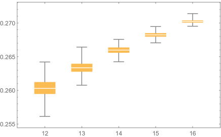
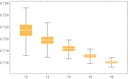
Figure 1: Box plots of the estimates $\widehat{\mathscr{R}}_{n}(Y)$ for $n=12,\dots,16$, based on 1,000 sample paths of fractional Brownian motion with $H=0.3$ (left), $H=0.7$ (right), and $Y$ as in (2.10).

As one can see from Figure 1, the estimator $\widehat{\mathscr{R}}_{n}$ performs relatively well but also exhibits a certain bias. This bias can be completely removed by passing to the scale-invariant estimator ${\mathscr{R}}^{s}_{n}$; see Figure 2.

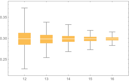
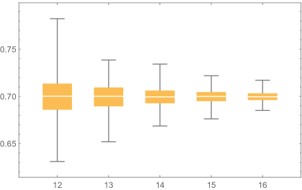
Figure 2: Box plots of the sequential scale estimates ${\mathscr{R}}^{s}_{n}(Y)$ for $n=12,\dots,16$, based on 1,000 sample paths of fractional Brownian motion with $H=0.3$ (left), $H=0.7$ (right), and $Y$ as in (2.10). The other parameters are chosen to be $m=3$ and $\alpha_{k}=1$ for $k=0,1,2,3$.

Now we apply our estimator $\widehat{\mathscr{R}}_{n}$ to a model in which log-volatility, $\log\sigma_{t}$, is given by a fractional Ornstein–Uhlenbeck process $X^{H}$ of the form

$$X^{H}_{t}=x_{0}+\rho\int_{0}^{t}(\mu-X^{H}_{s})\,ds+W^{H}_{t},\qquad t\in[0,1],$$

and we make discrete observations of the process

$$\int_{0}^{t}\sigma^{2}_{s}\,ds=\int_{0}^{t}e^{2X^{H}_{s}}\,ds,\qquad 0\leq t\leq 1.$$

To this end, we take again $N=n+6$ and simulate the values $X^{H}_{k2^{-N}}$ ($k=0,\dots,2^{N}$) by means of an Euler scheme. Then we put

$$Y^{\sigma}_{k2^{-n-2}}:=2^{-N}\sum_{j=1}^{2^{N-n-2}k}\exp\Big{(}2X^{H}_{j2^{-N}}\Big{)},\quad k=0,1,\dots,2^{n+2},$$ (2.11)

which is an approximation of $\int_{0}^{t}e^{2X^{H}_{s}}\,ds$ by Riemann sums. As one can see from Figure 3, the original estimator $\widehat{\mathscr{R}}_{n}$ performs rather poorly in this case, while the sequential scale estimator ${\mathscr{R}}^{s}_{n}$ performs almost as well as for the simple case $Y_{t}=\int_{0}^{t}W^{H}_{s}\,ds$. This is due to the fact that the function $g(t)=e^{2t}$ used in (2.11) distorts substantially the scale of the underlying process, but this distortion can be remedied by using the sequential scale estimator.

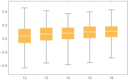
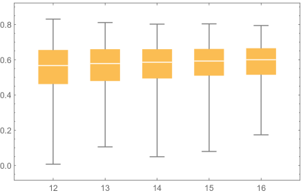
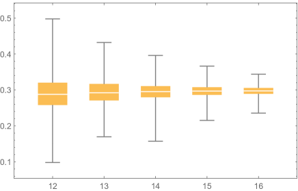
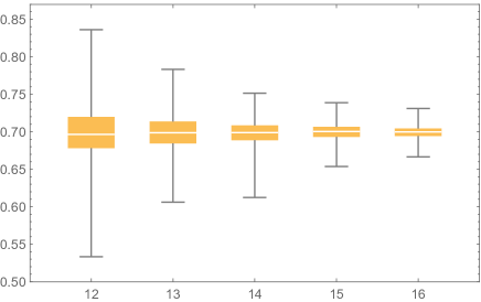
Figure 3: Box plots of the original estimates $\widehat{\mathscr{R}}_{n}(Y^{\sigma})$ (top) and the sequential scale estimates ${\mathscr{R}}^{s}_{n}(Y^{\sigma})$ (bottom) for $n=12,\dots,16$ based on 1,000 simulations of the antiderivative of the exponential Ornstein–Uhlenbeck process (2.11) with $H=0.3$ (left) and $H=0.7$ (right). The other parameters are chosen as $x_{0}=0$, $\rho=0.2$, $\mu=2$, $m=3$ and $\alpha_{k}=1$ for $k=0,1,\dots,3$.

3 Pathwise estimation

In this section, we formulate conditions on a single trajectory $x\in C[0,1]$ and its antiderivative $y(t)=\int_{0}^{t}x(s)\,ds$ under which the estimates $\widehat{\mathscr{R}}_{n}(y)$ converge to the roughness exponent of $x$. In Section 4, we will then verify that these conditions are satisfied for the typical sample paths of fractional Brownian motion. The results in the present section are hence of independent interest in situations in which it is not clear whether a given trajectory $x$ arises from fractional Brownian motion. We start by summarizing some key results and concepts from [14, 15] and also outline our rationale behind the specific form of the estimator $\widehat{\mathscr{R}}_{n}$.

3.1 The rationale behind the estimator $\widehat{\mathscr{R}}_{n}$

Recall that the Faber–Schauder functions are defined as

$$e_{-1,0}(t):=t,\quad e_{0,0}(t):=(\min\{t,1-t\})^{+},\quad e_{m,k}(t):=2^{-m/2}e_{0,0}(2^{m}t-k)$$

for $t\in\mathbb{R}$, $m\in\mathbb{N}$ and $k\in\mathbb{Z}$. It is well known that the restrictions of the Faber–Schauder functions to $[0,1]$ form a Schauder basis for $C[0,1]$. More precisely, our function $x\in C[0,1]$ can be uniquely represented as the uniform limit $x=\lim_{n}x_{n}$, where

$$x_{n}=x(0)+\left(x(1)-x(0)\right)e_{-1,0}+\sum_{m=0}^{n-1}\sum_{k=0}^{2^{m}-1}\theta_{m,k}e_{m,k},$$ (3.1)

and the Faber–Schauder coefficients $\theta_{m,k}$ are given by

$$\theta_{m,k}=2^{m/2}\left(2x\Big{(}\frac{2k+1}{2^{m+1}}\Big{)}-x\Big{(}\frac{k}{2^{m}}\Big{)}-x\Big{(}\frac{k+1}{2^{m}}\Big{)}\right).$$ (3.2)

As a matter of fact, it is easy to see that the function $x_{n}$ is simply the linear interpolation of $x$ based on the supporting grid $\mathbb{T}_{n}=\{k2^{-n}:k=0,\dots,2^{n}\}$.

In [14], we derived simple conditions under which the trajectory $x$ admits a roughness exponent ${R}\in[0,1]$ and also suggested a way in which ${R}$ can be estimated from discrete observations of $x$. Specifically, it follows from Theorem 2.4 and Proposition 4.1 in [14] that, if the Faber–Schauder coefficients satisfy the so-called reverse Jensen condition (see Definition 2.3 in [14]) and the sequence

$$\widehat{R}^{*}_{n}(x):=1-\frac{1}{n}\log_{2}\sqrt{\sum_{k=0}^{2^{n}-1}\theta_{n,k}^{2}}$$ (3.3)

converges to a finite limit $R$, then $x$ admits the roughness exponent $R$.

Note that it is assumed in [14] that the trajectory $x$ can be observed directly. This, however, is not the case in the context of our present paper, where $x$ is the (squared) volatility in a stochastic volatility model. So let us suppose now that we can only observe the values the antiderivative $y(t)=\int_{0}^{t}x(s)\,ds$ takes on the supporting grid $\mathbb{T}_{n+2}$. If we can interpolate the data points $\{y(t):t\in\mathbb{T}_{n+2}\}$ by means of a piecewise quadratic function $y_{n+2}\in C^{1}(\mathbb{R})$, then its derivative $y^{\prime}_{n+2}$ will be a continuous and piecewise linear function with supporting grid $\mathbb{T}_{n+1}$ and hence representable in the form

$$y^{\prime}_{n+2}=\hat{x}_{0}+\widehat{\theta}_{-1,0}e_{-1,0}+\sum_{m=0}^{n+1}\sum_{k=0}^{2^{m}-1}\widehat{\theta}_{m,k}e_{m,k}$$ (3.4)

for some initial value $\hat{x}_{0}$ and certain coefficients $\widehat{\theta}_{m,k}$. Such a piecewise quadratic $C^{1}$-interpolation $y_{n+2}$ exists in the form of the standard quadratic spline interpolation. Unfortunately, though, it is well known that quadratic spline interpolation suffers some serious drawbacks:

• the initial value $\hat{x}_{0}$ is not uniquely determined by the given data $\{y(t):t\in\mathbb{T}_{n+2}\}$;

• the values $y_{n+2}(t)$ depend in a highly sensitive manner on the choice of $\hat{x}_{0}$;

• the values $y_{n+2}(s)$ depend in a nonlocal way on the given data $\{y(t):t\in\mathbb{T}_{n+2}\}$, i.e., altering one data point $y(t)$ may affect the value $y_{n+2}(s)$ also if $s$ is located far away from $t$.

In [15], we investigate the analytical properties of the estimated Faber–Schauder coefficients $\widehat{\theta}_{m,k}$ defined in (3.4). It turns out that, when looking at quadratic spline interpolation through the lens of these coefficients, a miracle occurs. To see what happens, let us recall from [15, Theorem 2.1] the formula for the Faber–Schauder coefficients of $y^{\prime}_{n+2}$ for the generations $m=0,\dots,n$ and for generation $n+1$,

As one can see immediately from those formulas, the coefficients in generations $m=0,\dots n$ are independent of $\widehat{x}_{0}$, whereas the coefficients in generation $n+1$ contain the additive term $-2^{(n+1)/2+2}\hat{x}_{0}$, which translates any error made in estimating $\hat{x}_{0}$ into an $2^{(n+1)/2+2}$-fold error for each final-generation coefficient. Moreover, for $m=0,\dots n$, each $\widehat{\theta}_{m,k}$ depends only on those data points $y(t)$ for which $t$ belongs to the closure of the support of the corresponding wavelet function $e_{m,k}$. Thus, the entire nonlocality of the function $y_{n+2}$ arises from the coefficients in generation $n+1$, while the coefficients of all lower generations depend on locally on the given data. We refer to [15, Figure 2] for an illustration.

The main results in [15] concern error bounds for the estimated Faber–Schauder coefficients $\widehat{\theta}_{m,k}$. Specifically, we found that the $\ell_{2}$-norm of the combined errors in generations $m=0,\dots n$ is typically benign, whereas the error in the final generation $m=n+1$ can be larger than a factor of size $\mathcal{O}(2^{n})$ times the error of all previous generations combined. While the exact error bounds from [15] will not be needed in our present paper, the proof of Lemma 3.2 will rely on an algebraic representation of the error terms obtained in [15, Lemma 3.2] and stated in Equation 3.12 below.

The above-mentioned facts make it clear that the coefficients in generations $m=0,\dots n$ provide robust estimates for the corresponding true coefficients, while the estimates $\widehat{\theta}_{n+1,k}$ are highly non-robust and should be discarded. It is now obvious that in estimating the roughness exponent of $x$ from the data $\{y(t):t\in\mathbb{T}_{n+2}\}$, we should replace the true coefficients $\theta_{n,k}$ in our formula (3.3) for $\widehat{R}^{*}_{n}(x)$ with their estimates $\widehat{\theta}_{n,k}$. It remains to note that $\widehat{\theta}_{n,k}$ is in fact equal to $\vartheta_{n,k}$ defined in (2.5), so that we finally arrive at the rationale behind our estimator $\widehat{\mathscr{R}}_{n}$.

The following example provides a concrete instance where choosing the final-generation coefficients $\widehat{\theta}_{n+1,k}$ instead of $\vartheta_{n,k}=\widehat{\theta}_{n,k}$ leads to an estimate that is non-robust and also otherwise inferior.

Example 3.1.

For ${R}\in(0,1]$, let $x^{R}\in C[0,1]$ be the function with Faber–Schauder coefficients $\theta_{n,k}=2^{n(1/2-{R})}$. These functions belong to the well-studied class of fractal Takagi–Landsberg functions. It was shown in [19, Theorem 2.1] that $x^{R}$ has the roughness exponent ${R}$. Moreover, for $y^{R}(t)=\int_{0}^{t}x^{R}(s)\,ds$, it was shown in [15, Example 2.3] that the robust approximation (2.5) based on discrete observations of $y^{R}$ recovers exactly the Faber–Schauder coefficients of $x^{R}$. That is, for $n\in\mathbb{N}$ and $0\leq k\leq 2^{n}-1$, we have

$$\vartheta_{n,k}=\theta_{n,k}=2^{n(\frac{1}{2}-{R})}.$$

It follows that

$$\widehat{\mathscr{R}}_{n}(y^{R})=1-\frac{1}{n}\log_{2}\sqrt{\sum_{k=0}^{2^{n}-1}2^{(1-2{R})n}}=1-\frac{1}{n}\log_{2}2^{(1-{R})n}={R}.$$

Hence, the estimator $\widehat{\mathscr{R}}_{n}$ is not only consistent but also exact in the sense that it gives the correct value ${R}$ for every finite $n$.

Now we replace $\vartheta_{n,k}=\widehat{\theta}_{n,k}$ with the final-generation estimates $\widehat{\theta}_{n+1,k}$ as defined in (3.6). Note that this requires the choice of an initial value $\hat{x}_{0}$. The corresponding estimator is given by

$$\widetilde{\mathscr{R}}_{n}(y^{R}):=1-\frac{1}{n+1}\log_{2}\sqrt{\sum_{k=0}^{2^{n+1}-1}\widehat{\theta}_{n+1,k}^{2}}.$$

We get from [15, Example 3.2] that for ${R}<1/2$,

$$\widehat{\theta}_{n+1,k}=-2^{(n+1)/2+2}\hat{x}_{0}+\sum_{m=n+1}^{\infty}2^{m(\frac{1}{2}-{R})}=-2^{(n+1)/2+2}\hat{x}_{0}+\frac{2^{(n+1)(\frac{1}{2}-{R})}}{1-2^{\frac{1}{2}-{R}}}.$$

Hence,

$$\sqrt{\sum_{k=0}^{2^{n+1}-1}\widehat{\theta}_{n+1,k}^{2}}=2^{n+1}\left|-4\hat{x}_{0}+\frac{2^{-(n+1){R}}}{1-2^{\frac{1}{2}-{R}}}\right|.$$

It follows that

$$\lim_{n\uparrow\infty}\widetilde{\mathscr{R}}_{n}(y^{R})=\begin{cases}0&\text{if $\hat{x}_{0}\neq 0$,}\\ {R}&\text{if $\hat{x}_{0}=0$.}\end{cases}$$

This shows that the estimator $\widetilde{\mathscr{R}}_{n}$ is extremely sensitive with respect to the estimate $\hat{x}_{0}$ of the exact initial value $x(0)$, which in typical applications will be unknown. Even in the case that $x(0)$ is known, the correct value ${R}$ is only obtained asymptotically, whereas $\widehat{\mathscr{R}}_{n}(y^{R})={R}$ for all finite $n$. These observations illustrate once again why we deliberately discard the final generation $\widehat{\theta}_{n+1,k}$ of estimated Faber–Schauder coefficients.

3.2 Pathwise consistency of $\widehat{\mathscr{R}}_{n}(y)$

Let us fix $x\in C[0,1]$ and denote by $\theta_{m,k}$ its Faber–Schauder coefficients (3.2). As before, we denote by $y(t)=\int_{0}^{t}x(s)\,ds$ the antiderivative of $x$ and by $\vartheta_{n,k}$ the coefficients defined in (2.5). To be consistent with [15], we introduce the following vector notation,

$$\bar{\bm{\theta}}_{n}:=\big{(}\theta_{n,0},\theta_{n,1}\cdots,\theta_{n,2^{n}}\big{)}^{\top}\in\mathbb{R}^{2^{n}}\quad\text{and}\quad\bar{\bm{\vartheta}}_{n}=\big{(}\vartheta_{n,0},\vartheta_{n,1}\cdots,\vartheta_{n,2^{n}-1}\big{)}^{\top}\in\mathbb{R}^{2^{n}},$$ (3.7)

Then the estimators $\widehat{R}^{*}_{n}$ and $\widehat{\mathscr{R}}_{n}$ defined in (3.3) and (2.6) can be written as

$$\widehat{R}_{n}^{*}(x)=1-\frac{1}{n}\log_{2}\|\bar{\bm{\theta}}_{n}\|_{\ell_{2}}\quad\text{and}\quad\widehat{\mathscr{R}}_{n}(y)=1-\frac{1}{n}\log_{2}\|\bar{\bm{\vartheta}}_{n}\|_{\ell_{2}}.$$ (3.8)

Following [15], we introduce the column vector $\bm{z}_{n}:=(z^{(n)}_{i})_{1\leq i\leq 2^{n}}$ with components

$$z^{(n)}_{i}=2^{3n/2}\sum_{m=n}^{\infty}2^{-3m/2}\sum_{k=0}^{2^{m-n}-1}\theta_{m,k+2^{m-n}(i-1)}\quad\text{for}\quad 1\leq i\leq 2^{n}.$$ (3.9)

As observed in [15], the infinite series in (3.9) converges absolutely if $x$ satisfies a Hölder condition, and for simplicity we are henceforth going to make this assumption. For $1\leq i,j\leq 2^{n}$, we let furthermore

$$\bm{\eta}_{i,j}=\begin{cases}\bm{r}&\quad\text{for}\quad 1\leq i=j\leq 2^{n},\\ \bm{0}_{1\times 4}&\quad\text{for}\quad 1\leq i\neq j\leq 2^{n},\end{cases}$$ (3.10)

where $\bm{r}:=\frac{1}{4}(-1,+1,+1,-1)$, and $\bm{0}_{m\times n}$ denotes the $m\times n$-dimensional zero matrix. Moreover, we denote

$$Q_{n}:=\left[\begin{array}[]{c c c c c}\bm{\eta}_{1,1}&\bm{\eta}_{1,2}&\cdots&\bm{\eta}_{1,2^{n}-1}&\bm{\eta}_{1,2^{n}}\\ \bm{\eta}_{2,1}&\bm{\eta}_{2,2}&\cdots&\bm{\eta}_{2,2^{n}-1}&\bm{\eta}_{2,2^{n}}\\ \vdots&\vdots&\ddots&\vdots&\vdots\\ \bm{\eta}_{2^{n},1}&\bm{\eta}_{2^{n},2}&\cdots&\bm{\eta}_{2^{n},2^{n}-1}&\bm{\eta}_{2^{n},2^{n}}\\ \end{array}\right]\in\mathbb{R}^{2^{n}\times 2^{n+2}}.$$ (3.11)

It was shown in [15, Lemma 3.2] that the error between the true and estimated Faber–Schauder coefficients can be represented as follows,

$$\bar{\bm{\vartheta}}_{n}-\bar{\bm{\theta}}_{n}=\bm{w}_{n},\quad\text{where}\quad\bm{w}_{n}=Q_{n}\bm{z}_{n+2}\in\mathbb{R}^{2^{n}}.$$ (3.12)

Consider the following condition:

$$\text{There exists $\kappa\in\mathbb{R}\setminus\{1\}$ such that}\quad\frac{\left\lVert{\bm{w}_{n}}\right\rVert_{\ell_{2}}}{\|\bar{\bm{\theta}}_{n}\|_{\ell_{2}}}\longrightarrow\kappa\quad\text{as $n\uparrow\infty$.}$$ (3.13)

We will see in Proposition 4.1 that condition (3.13) is $\mathbb{P}$-a.s. satisfied for fractional Brownian motion.

Lemma 3.2.

Under condition (3.13), there exist $n_{0}\in\mathbb{N}$ and constants $0<\kappa_{-}\leq\kappa_{+}<\infty$ such that

$$\kappa_{-}\|\bar{\bm{\theta}}_{n}\|_{\ell_{2}}\leq\left\lVert{\bar{\bm{\vartheta}}_{n}}\right\rVert_{\ell_{2}}\leq\kappa_{+}\|\bar{\bm{\theta}}_{n}\|_{\ell_{2}}\quad\text{for all $n\geq n_{0}$.}$$ (3.14)

Proof.

Let $\kappa$ be as in (3.13). Then, for any $\varepsilon<|\kappa-1|/2$, there exists $n_{\varepsilon}\in\mathbb{N}$ such that for $n\geq n_{\varepsilon}$, we have $\left\lVert{\bar{\bm{\theta}}_{n}}\right\rVert_{\ell_{2}}(\kappa-\varepsilon)<\left\lVert{\bm{w}_{n}}\right\rVert_{\ell_{2}}<\left\lVert{\bar{\bm{\theta}}_{n}}\right\rVert_{\ell_{2}}(\kappa+\varepsilon)$. Using the representation (3.12) and applying the triangle inequality gives

$$\left\lVert{\bar{\bm{\vartheta}}_{n}}\right\rVert_{\ell_{2}}=\left\lVert{\bar{\bm{\theta}}_{n}-\bm{w}_{n}}\right\rVert_{\ell_{2}}\leq\left\lVert{\bar{\bm{\theta}}_{n}}\right\rVert_{\ell_{2}}+\left\lVert{\bm{w}_{n}}\right\rVert_{\ell_{2}}\leq(\kappa+\varepsilon+1)\left\lVert{\bar{\bm{\theta}}_{n}}\right\rVert_{\ell_{2}}.$$

On the other hand, we have

$$\left\lVert{\bar{\bm{\vartheta}}_{n}}\right\rVert_{\ell_{2}}=\left\lVert{\bar{\bm{\theta}}_{n}-\bm{w}_{n}}\right\rVert_{\ell_{2}}\geq\Big{|}\left\lVert{\bar{\bm{\theta}}_{n}}\right\rVert_{\ell_{2}}-\left\lVert{\bm{w}_{n}}\right\rVert_{\ell_{2}}\Big{|}\geq\big{(}|1-\kappa-\varepsilon|\wedge|1-\kappa+\varepsilon|\big{)}\left\lVert{\bar{\bm{\theta}}_{n}}\right\rVert_{\ell_{2}}.$$

This completes the proof. ∎

By taking logarithms in (3.14), Lemma 3.2 immediately yields the following result.

Proposition 3.3.

Under condition (3.13), the limit $\lim_{n}\widehat{\mathscr{R}}_{n}(y)$ exists if and only if $\lim_{n}\widehat{R}^{*}_{n}(x)$ exists. Moreover, in this case, $\lim_{n}\widehat{\mathscr{R}}_{n}(y)=\lim_{n}\widehat{R}^{*}_{n}(x)$.

Example 3.4.

In the situation of Example 3.1, we have seen that $\vartheta_{n,k}=\theta_{n,k}=2^{n(\frac{1}{2}-{R})}$. Applying the representation (3.12) yields that $\bm{w}_{n}=\bm{0}_{2^{n}\times 1}$. This implies $\lim_{n}\left\lVert{\bm{w}_{n}}\right\rVert_{\ell_{2}}/\|\bar{\bm{\theta}}_{n}\|_{\ell_{2}}=0$. That is, $x^{R}$ satisfies condition (3.13). Hence, Proposition 3.3 applies, which gives an additional proof of the previously observed fact that $\lim_{n}\widehat{\mathscr{R}}_{n}(y)={R}$.

Next, we consider the following question: Under which conditions on $x$ and $g$ does $u:=g\circ x$ admit the roughness exponent ${R}$? To answer this question, we fix the following notation throughout the remainder of this section,

$$u(t)=g(x(t))\qquad\text{and}\qquad v(t)=\int_{0}^{t}u(s)\,ds=\int_{0}^{t}g(x(s))\,ds.$$ (3.15)

Proposition 3.5.

If $x$ admits the roughness exponent ${R}$, $g$ belongs to $C^{1}(\mathbb{R})$, and $g^{\prime}$ is nonzero on the range $x([0,1])$ of $x$, then $u=g\circ x$ also admits the roughness exponent ${R}$.

Proof.

For any $p>0$, the mean value theorem and the intermediate value theorem yield numbers $\tau_{n,k}\in[k2^{-n},(k+1)2^{-n}]$ such that

$$\begin{split}\langle u\rangle^{(p)}_{n}&=\sum_{k=0}^{2^{n}-1}\left|g^{\prime}(x(\tau_{n,k}))\Big{(}x\Big{(}\frac{k+1}{2^{n}}\Big{)}-x\Big{(}\frac{k}{2^{n}}\Big{)}\Big{)}\right|^{p}=\sum_{k=0}^{2^{n}-1}\left|g^{\prime}(x(\tau_{n,k}))\right|^{p}\left|x\Big{(}\frac{k+1}{2^{n}}\Big{)}-x\Big{(}\frac{k}{2^{n}}\Big{)}\right|^{p},\end{split}$$ (3.16)

where the notation $\langle u\rangle^{(p)}_{n}$ was introduced in (2.3). Since $g^{\prime}$ is continuous and nonzero, there are constants $0<c_{-}<c_{+}<\infty$ such that $c_{-}\leq|g^{\prime}(x(t))|\leq c_{+}$ for all $t\in[0,1]$. Hence, $c_{-}^{p}\langle x\rangle^{(p)}_{n}\leq\langle u\rangle^{(p)}_{n}\leq c_{+}^{p}\langle x\rangle^{(p)}_{n}$ holds for all $n$. Passing to the limit $n\uparrow\infty$ for $p>1/{R}$ and $p<1/{R}$ yields the result. ∎

Now we turn to the following question: Under which conditions do we have $\widehat{\mathscr{R}}_{n}(v)\to{R}$, where $v$ is as in (3.15)? The conditions we are going to introduce for answering this question are relatively strong. Nevertheless, they hold for the sample paths of fractional Brownian motion.

Proposition 3.6.

Suppose there exists ${R}\in(0,1)$ such that the following conditions hold.

1. We have

   $$0<\liminf_{n\uparrow\infty}2^{n(2{R}-2)}\sum_{k=0}^{2^{n}-1}\vartheta_{n,k}^{2}\leq\limsup_{n\uparrow\infty}2^{n(2{R}-2)}\sum_{k=0}^{2^{n}-1}\vartheta_{n,k}^{2}<\infty.$$ (3.17)

2. The function $x$ is Hölder continuous with exponent $\alpha\in(2{R}/5,1]$.

Then, if $g\in C^{2}(\mathbb{R})$ is strictly monotone, we have $\lim_{n}\widehat{\mathscr{R}}_{n}(v)={R}$.

Proof.

In this proof, we will work with the actual and estimated Faber–Schauder coefficients of the various functions $x$, $y$, $u$, and $v$. For this reason, we will temporarily use a superscript to indicate from which function the Faber–Schauder coefficients will be computed. That is, for any function $f$, we write

$$\begin{split}\theta^{f}_{n,k}&=2^{n/2}\left(2f\Big{(}\frac{2k+1}{2^{n+1}}\Big{)}-f\Big{(}\frac{k}{2^{n}}\Big{)}-f\Big{(}\frac{k+1}{2^{n}}\Big{)}\right),\\ \vartheta^{f}_{n,k}&=2^{3n/2+3}\left(f\Big{(}\frac{4k}{2^{n+2}}\Big{)}-2f\Big{(}\frac{4k+1}{2^{n+2}}\Big{)}+2f\Big{(}\frac{4k+3}{2^{n+2}}\Big{)}-f\Big{(}\frac{4k+4}{2^{n+2}}\Big{)}\right).\end{split}$$ (3.18)

With this notation, the coefficients $\vartheta_{n,k}$ in (2.5) should be re-written as $\vartheta_{n,k}^{y}$. In particular, (3.17) refers to the coefficients $\vartheta^{y}_{n,k}$. Our goal in this proof is to show that (3.17) carries over to the coefficients $\vartheta^{v}_{n,k}$. That is,

$$0<\liminf_{n\uparrow\infty}2^{n(2{R}-2)}\sum_{k=0}^{2^{n}-1}\big{(}\vartheta^{v}_{n,k}\big{)}^{2}\leq\limsup_{n\uparrow\infty}2^{n(2{R}-2)}\sum_{k=0}^{2^{n}-1}\big{(}\vartheta^{v}_{n,k}\big{)}^{2}<\infty.$$ (3.19)

Taking logarithms, dividing by $2n$, and passing to the limit will then yield ${R}-\widehat{\mathscr{R}}_{n}(v)\to 0$, which is the assertion.

It remains to establish (3.19). Rewriting the second line in (3.18) gives after a short computation that

$$\vartheta^{f}_{n,k}=2^{n+5/2}\left(\theta^{f}_{n+1,2k+1}-\theta^{f}_{n+1,2k}\right).$$ (3.20)

Let us introduce the notation $\theta_{m,k}^{f}(s):=\theta_{m.k}^{f(s+\cdot)}$. That is, $\theta_{m,k}^{f}(s)$ are the Faber–Schauder coefficients of the function $t\mapsto f(s+t)$ for given $s\geq 0$. One can avoid undefined arguments of functions in case $s+t>1$ by assuming without loss of generality that all occurring functions on $[0,1]$ are in fact defined on all of $[0,\infty)$. With this notation, we get from (3.20) that for $f\in C^{1}[0,\infty)$,

$$\vartheta^{f}_{n,k}=2^{n+5/2}\int_{0}^{2^{-n-1}}\theta^{f^{\prime}}_{n+1,2k}(s)\,ds.$$ (3.21)

Applying the mean-value theorem and the intermediate value theorem yields certain intermediate times $\tau_{n+2,k}(s)\in[2^{-n-2}k+s,2^{-n-2}(k+1)+s]$ such that for $s\in[0,2^{-n-1}]$,

$$\begin{split}\theta^{u}_{n+1,2k}(s)&=2^{(n+1)/2}\left(2u\Big{(}\frac{4k+1}{2^{n+2}}+s\Big{)}-u\Big{(}\frac{4k}{2^{n+2}}+s\Big{)}-u\Big{(}\frac{4k+2}{2^{n+2}}+s\Big{)}\right)\\ &=2^{(n+1)/2}g^{\prime}\big{(}x(\tau_{n+2,4k}(s))\big{)}\left(x\Big{(}\frac{4k+1}{2^{n+2}}+s\Big{)}-x\Big{(}\frac{4k}{2^{n+2}}+s\Big{)}\right)\\ &+2^{(n+1)/2}g^{\prime}\big{(}x(\tau_{n+2,4k+1}(s))\big{)}\left(x\Big{(}\frac{4k+1}{2^{n+2}}+s\Big{)}-x\Big{(}\frac{4k+2}{2^{n+2}}+s\Big{)}\right),\\ &=2^{(n+1)/2}\scalebox{0.9}{\mbox{$\displaystyle\left(\frac{g^{\prime}\big{(}x(\tau_{n+2,4k}(s))\big{)}+g^{\prime}\big{(}x(\tau_{n+2,4k+1}(s))\big{)}}{2}\left(2x\Big{(}\frac{4k+1}{2^{n+2}}+s\Big{)}-x\Big{(}\frac{4k}{2^{n+2}}+s\Big{)}-x\Big{(}\frac{4k+2}{2^{n+2}}+s\Big{)}\right)\right)$}}\\ &\quad+2^{(n+1)/2}\left(\frac{g^{\prime}\big{(}x(\tau_{n+2,4k}(s))\big{)}-g^{\prime}\big{(}x(\tau_{n+2,4k+1}(s))\big{)}}{2}\left(x\Big{(}\frac{4k+2}{2^{n+2}}+s\Big{)}-x\Big{(}\frac{4k}{2^{n+2}}+s\Big{)}\right)\right).\end{split}$$

The intermediate value theorem and the mean-value theorem also imply that there are intermediate times $\tau^{\sharp}_{n+1,2k}(s),\tau^{\flat}_{n+1,2k}(s)\in[2^{-n-1}2k+s,2^{-n-1}(2k+1)+s]$ such that

$$\frac{1}{2}\left(g^{\prime}\big{(}x(\tau_{n+2,4k}(s))\big{)}+g^{\prime}\big{(}x(\tau_{n+2,4k+1}(s))\big{)}\right) =g^{\prime}\big{(}\tau^{\sharp}_{n+1,2k}(s)\big{)},$$

$$\frac{1}{2}\left(g^{\prime}\big{(}x(\tau_{n+2,4k}(s))\big{)}-g^{\prime}\big{(}x(\tau_{n+2,4k+1}(s))\big{)}\right) =\frac{1}{2}g^{\prime\prime}\big{(}\tau^{\flat}_{n+1,2k}(s)\big{)}\left(x(\tau_{n+2,4k}(s))-x(\tau_{n+2,4k+1}(s))\right).$$

With the shorthand notation

$$\zeta^{x}_{n+1,2k}(s):=2^{(n+1)/2}\left(x\Big{(}\frac{4k+2}{2^{n+2}}+s\Big{)}-x\Big{(}\frac{4k}{2^{n+2}}+s\Big{)}\right)\big{(}x(\tau_{n+2,4k}(s))-x(\tau_{n+2,4k+1}(s))\big{)},$$

we then have

$$\theta^{u}_{n+1,2k}(s)=g^{\prime}\big{(}\tau^{\sharp}_{n+1,2k}(s)\big{)}\theta^{x}_{n+1,2k}(s)+g^{\prime\prime}\big{(}\tau^{\flat}_{n+1,2k}(s)\big{)}\zeta^{x}_{n+1,2k}(s).$$

Plugging the preceding equation into (3.21) and applying the mean value theorem for integrals yields intermediate times $\tau^{\sharp}_{n+1,k},\tau^{\flat}_{n+1,k}\in[2^{-n-1}{k},2^{-n-1}(k+1)]$ that are independent of $s$ such that

$$\begin{split}\vartheta^{v}_{n,k}&=2^{n+5/2}g^{\prime}\big{(}x(\tau^{\sharp}_{n+1,2k})\big{)}\int_{0}^{2^{-n-1}}\theta^{x}_{n+1,2k}(s)\,ds+2^{n+5/2}g^{\prime\prime}\big{(}x(\tau^{\flat}_{n+1,2k})\big{)}\int_{0}^{2^{-n-1}}\zeta^{x}_{n+1,2k}(s)\,ds\\ &=g^{\prime}\big{(}x(\tau^{\sharp}_{n+1,2k})\big{)}\vartheta^{y}_{n,k}+2^{n+5/2}g^{\prime\prime}\big{(}x(\tau^{\flat}_{n+1,2k})\big{)}\int_{0}^{2^{-n-1}}\zeta^{x}_{n+1,2k}(s)\,ds.\end{split}$$

Introducing the shorthand notation

$$\widetilde{\zeta}^{x}_{n+1,2k}:=2^{n+5/2}\int_{0}^{2^{-n-1}}\zeta^{x}_{n+1,2k}(s)\,ds,$$

and let us write

$$\begin{split}\big{(}\vartheta^{v}_{n,k}\big{)}^{2}&=\big{(}g^{\prime}\big{(}x(\tau^{\sharp}_{n+1,2k})\big{)}\big{)}^{2}\big{(}\vartheta^{y}_{n,k}\big{)}^{2}+\left(g^{\prime\prime}\big{(}x(\tau^{\flat}_{n+1,2k})\big{)}\right)^{2}\big{(}\widetilde{\zeta}^{x}_{n+1,2k}\big{)}^{2}\\ &\qquad+2g^{\prime}\big{(}x(\tau^{\sharp}_{n+1,2k})\big{)}g^{\prime\prime}\big{(}x(\tau^{\flat}_{n+1,2k})\big{)}\vartheta^{y}_{n,k}\widetilde{\zeta}^{x}_{n+1,2k}.\end{split}$$ (3.22)

For each of the three terms on the right, we will now analyze its contribution to the quantities in (3.19). The main contribution comes from the first term on the right. Indeed, our assumptions on $g$ imply that there are constants $0<c_{-}\leq c_{+}<\infty$ such that $c_{-}<(g^{\prime}(x(t)))^{2}<c^{+}$ for all $t\in[0,1]$, and so

$$c_{-}2^{n(2{R}-2)}\sum_{k=0}^{2^{n}-1}\big{(}\vartheta^{y}_{n,k}\big{)}^{2}\leq 2^{n(2{R}-2)}\sum_{k=0}^{2^{n}-1}\big{(}\vartheta^{v}_{n,k}\big{)}^{2}\leq c_{+}2^{n(2{R}-2)}\sum_{k=0}^{2^{n}-1}\big{(}\vartheta^{y}_{n,k}\big{)}^{2}.$$

This will establish (3.19) as soon as we have shown that the contributions of the two remaining terms in (3.22) are asymptotically negligible. For the second term, we use the Hölder continuity of $x$ to get a constant $c_{x}$ for which

$$|x(\tau_{n+2,4k}(s))-x(\tau_{n+2,4k+1}(s))|\leq c_{x}|\tau_{n+2,4k}(s)-\tau_{n+2,4k+1}(s)|^{\alpha}\leq c_{x}2^{-\alpha n}$$

Furthermore, there exists $\kappa_{x}>0$ such that $32(g^{\prime\prime}(x(s)))^{2}\leq\kappa_{x}$ for all $s\in[0,1]$. Then,

$$\begin{split}&2^{(2{R}-2)n}\sum_{k=0}^{2^{n}-1}\left(g^{\prime\prime}\big{(}x(\tau^{\flat}_{n+1,2k})\big{)}\right)^{2}\left(\widetilde{\zeta}_{n+1,2k}\right)^{2}\\ &=2^{(2{R}-2)n}\sum_{k=0}^{2^{n}-1}\left(g^{\prime\prime}\big{(}x(\tau^{\flat}_{n+1,2k})\big{)}\right)^{2}\left(2^{n+5/2}\int_{0}^{2^{-n-1}}\zeta^{x}_{n+1,2k}(s)\,ds\right)^{2}\\ &\leq\kappa_{x}2^{2{R}n}\sum_{k=0}^{2^{n}-1}\left(\int_{0}^{2^{-n-1}}\zeta^{x}_{n+1,2k}(s)\,ds\right)^{2}\leq\kappa_{x}2^{2{R}n}\sum_{k=0}^{2^{n}-1}2^{-n-1}\int_{0}^{2^{-n-1}}\left(\zeta^{x}_{n+1,2k}(s)\right)^{2}\,ds\\ &\leq\kappa_{x}2^{(2{R}-1)n}\int_{0}^{2^{-n-1}}\sum_{k=0}^{2^{n}-1}\left(x\Big{(}\frac{4k+2}{2^{n+2}}+s\Big{)}-x\Big{(}\frac{4k}{2^{n+2}}+s\Big{)}\right)^{2}\left(x(\tau_{n+2,4k}(s))-x(\tau_{n+2,4k+1}(s))\right)^{2}\,ds\\ &=\kappa_{x}2^{\alpha n}\int_{0}^{2^{-n-1}}2^{(2{R}-1-\alpha)n}\sum_{k=0}^{2^{n}-1}\left(x\Big{(}\frac{2k+1}{2^{n+1}}+s\Big{)}-x\Big{(}\frac{2k}{2^{n+1}}+s\Big{)}\right)^{2}\big{(}c^{2}_{x}2^{-2\alpha n}\big{)}\,ds\\ &\leq\kappa_{x}c^{2}_{x}\int_{0}^{2^{-n-1}}\sup_{s\in[0,2^{-n-1}]}\left(2^{(2{R}-1-3\alpha)n}\sum_{k=0}^{2^{n+1}-1}\left(x\Big{(}\frac{2k+1}{2^{n+1}}+s\Big{)}-x\Big{(}\frac{2k}{2^{n}}+s\Big{)}\right)^{2}\right)\,ds.\end{split}$$

Moreover, (b) implies the integrand in the final term converges to zero:

$$\lim_{n\uparrow\infty}\sup_{0\leq s\leq 2^{-n-1}}2^{(2{R}-1-3\alpha)n}\sum_{k=0}^{2^{n+1}-1}\left(x\Big{(}\frac{2k+1}{2^{n+1}}+s\Big{)}-x\Big{(}\frac{2k}{2^{n}}+s\Big{)}\right)^{2}=0.$$ (3.23)

Indeed, by the Hölder continuity of $x$, we can again use the constant $c_{x}$ to get

$$2^{(2{R}-1-3\alpha)n}\sum_{k=0}^{2^{n+1}-1}\left(x\Big{(}\frac{2k+1}{2^{n+1}}+s\Big{)}-x\Big{(}\frac{2k}{2^{n}}+s\Big{)}\right)^{2} \leq 2^{(2{R}-1-3\alpha)n}\cdot 2^{n+1}\cdot c_{x}^{2}2^{-2(n+1)\alpha};$$

the right-hand side is equal to $c_{x}^{2}\cdot 2^{1-2\alpha}\cdot 2^{(2{R}-5\alpha)n}$, which converges to zero as $n\uparrow\infty$. Altogether, this shows that the contribution of the second term on the right-hand side of (3.22) is negligible.

For the cross-product term on the rightmost side of (3.22), we get from the Cauchy–Schwarz inequality,

$$\begin{split}\@ADDCLASS{ltx_eqn_lefteqn}$\displaystyle\lim_{n\uparrow\infty}2^{(2{R}-2)n}\sum_{k=0}^{2^{n}-1}g^{\prime}\big{(}x(\tau^{\sharp}_{n+1,2k})\big{)}g^{\prime\prime}\big{(}x(\tau^{\flat}_{n+1,2k})\big{)}\vartheta_{n,k}\widetilde{\zeta}^{x}_{n+1,2k}$\mbox{}\hfil\\ &\leq\sqrt{\lim_{n\uparrow\infty}2^{(2{R}-2)n}\sum_{k=0}^{2^{n}-1}\left(g^{\prime}\big{(}x(\tau^{\sharp}_{n+1,2k})\big{)}\right)^{2}\big{(}\vartheta_{n,k}\big{)}^{2}}\sqrt{\lim_{n\uparrow\infty}2^{(2{R}-2)n}\sum_{k=0}^{2^{n}-1}\left(g^{\prime\prime}\big{(}x(\tau^{\flat}_{n+1,2k})\big{)}\right)^{2}\big{(}\widetilde{\zeta}^{x}_{n+1,2k}\big{)}^{2}}=0.\end{split}$$

Altogether, (3.19) follows.∎

To conclude this section, we state and prove a lemma, which will be needed for the proof of Proposition 4.1. For possible future reference, we include it into our present pathwise context. For $n,k\in\mathbb{N}$, let us consider the vector $\bm{z}_{(n,k)}=(z^{(n,k)}_{i})\in\mathbb{R}^{2^{n}}$, where

$$z^{(n,k)}_{i}=2^{3n/2}\sum_{m=n}^{n+k}2^{-3m/2}\sum_{j=0}^{2^{m-n}-1}\theta_{m,j+2^{m-n}(i-1)}\quad\text{for}\quad 1\leq i\leq 2^{n}.$$ (3.24)

It is clear that the vector $\bm{z}_{(n,k)}$ is a truncated version of the vector $\bm{z}_{n}$ defined in (3.9). Since each Faber–Schauder coefficient $\theta_{m,k}$ is a linear combination of the values $x(j2^{-n-k-1})$, each $z^{(n,k)}_{i}$ must admit the following representation,

$$z^{(n,k)}_{i}=\sum_{j=0}^{2^{n+k+1}}\xi^{(n,k,i)}_{j}x\Big{(}\frac{j}{2^{n+k+1}}\Big{)},$$ (3.25)

for certain coefficients $\xi^{(n,k,i)}_{j}$. The following lemma computes the values of these coefficients.

Lemma 3.7.

We have

$$\xi_{j}^{(n,k,i)}=\begin{cases}0&\quad\text{if}\quad j\leq 2^{k+1}(i-1)-1\quad\text{or}\quad j\geq 2^{k+1}i+1,\\ 2^{n/2}(2^{-k}-2)&\quad\text{if}\quad j=2^{k+1}(i-1)\quad\text{or}\quad j=2^{k+1}i,\\ 2^{1-k+n/2}&\quad\text{if}\quad 2^{k+1}(i-1)+1\leq j\leq 2^{k}i-1.\end{cases}$$ (3.26)

Proof of Lemma 3.7.

We fix $n\in\mathbb{N}$ and $1\leq i\leq 2^{n}$ and proceed by induction on $k\in\mathbb{N}$. First, let us establish the base case $k=0$. Then

$$z^{(n,0)}_{i}=\theta_{n,i-1}=2^{n/2+1}x\Big{(}\frac{2i-1}{2^{n+1}}\Big{)}-2^{n/2}x\Big{(}\frac{2i}{2^{n+1}}\Big{)}-2^{n/2}x\Big{(}\frac{2i-2}{2^{n+1}}\Big{)}.$$ (3.27)

Moreover, plugging $k=0$ into (3.26) yields that $\xi_{2i-2}^{(n,0,i)}=\xi_{2i}^{(n,0,i)}=-2^{n/2}$, $\xi_{2i-1}^{(n,0,i)}=2^{n/2+1}$ and $\xi_{j}^{(n,0,i)}=0$ otherwise. It is clear that those coefficients coincide with the corresponding ones in (3.27), which proves our induction for the initial step $k=0$.

Next, let us assume that (3.26) holds for $k=m$ and subsequently prove that this identity also holds for $k=m+1$. It follows from (3.24) that

$$z^{(n,m+1)}_{i}=z^{(n,m)}_{i}+2^{n/2-m-1}\sum_{j=2^{m+1}(i-1)}^{2^{m+1}i-1}\bigg{(}2x\Big{(}\frac{2j+1}{2^{n+m+2}}\Big{)}-x\Big{(}\frac{j}{2^{n+m+1}}\Big{)}-x\Big{(}\frac{j+1}{2^{n+m+1}}\Big{)}\bigg{)}.$$ (3.28)

For $2^{m+1}(i-1)<j<2^{m+1}i-1$, the point $2^{-n-m-2}(2j+1)$ cannot be written in the form $\ell 2^{-n-m-1}$ for some $\ell\in\mathbb{N}_{0}$. Hence

$$\xi_{2j+1}^{(n,m+1,i)}=2\cdot 2^{n/2-m-1}=2^{n/2-m},$$

as the term $x(2^{-n-m-2}(2j+1))$ does not appear in the linear combination (3.25) for $k=m$. Next, for $2^{k-n}(i-1)<j<2^{k-n}i$, the point $2^{-n-m-2}2j=2^{-n-m-1}j$ can be written in the form $\ell 2^{-n-m-1}$ for some $\ell\in\mathbb{N}_{0}$. It thus follows from (3.25) and (3.26) that

$$\xi^{(n,m+1,i)}_{2j}=\xi^{(n,m,i)}_{j}-2\cdot 2^{n/2-m-1}=2^{n/2-m},$$

as the term $x(2^{-n-m-1}j)$ contributes to the representation of $\bm{z}^{(n,m)}_{i}$ with $\xi^{(n,m,i)}_{j}=2^{n/2-m+1}$. Moreover, for $j=2^{k-n}(i-1)$ or $j=2^{k-n}i$, we have

$$\xi_{j}^{(n,m+1,i)}=\xi_{j}^{(n,m,i)}-2^{n/2-m-1}=2^{n/2}(2^{-m}-2)-2^{n/2-m-1}=2^{n/2}(2^{-m-1}-2).$$

Last, for $j\leq 2^{m+2}(i-1)-1$ or $j\geq 2^{m+2}i+1$, the term $x(2^{-n-m-2})$ does not appear on right-hand side of (3.28). Thus, we have $\xi_{j}^{(n,m+1,i)}=0$. Comparing the above identities with (3.26) proves the case for $k=m+1$. ∎

4 Proof of Theorem 2.1

Proof of Theorem 2.1.

It was shown in [14, Theorem 5.1] that $W^{H}$ admits $\mathbb{P}$-a.s. the roughness exponent $H$. It now follows from Proposition 3.5 that the sample paths of $X=g(W^{H})$ also admit the roughness exponent $H$.

Now we prove that, with probability one, $\widehat{\mathscr{R}}_{n}(X)\to H$. To this end, we use the following result by Gladyshev [13] on the convergence of the weighted quadratic variation of $W^{H}$,

$$2^{(2H-1)n}\langle W^{H}\rangle_{n}^{(2)}\longrightarrow 1\quad\text{$\mathbb{P}$-a.s.}$$

Hence, if $\bar{\bm{\theta}}_{n}=(\theta_{n,k})$ are the Faber–Schauder coefficients of the sample paths of $W^{H}$, then [14, Proposition 4.1] yields that

$$2^{(2H-2)n}\left\lVert{\bar{\bm{\theta}}_{n}}\right\rVert_{\ell_{2}}^{2}=2^{(2H-2)n}\sum_{k=0}^{2^{n}-1}\theta^{2}_{n,k}\longrightarrow 2^{2-2H}-1\quad\text{$\mathbb{P}$-a.s.}$$ (4.1)

Lemma 3.2 now implies that condition (a) of Proposition 3.6 is satisfied. Condition (b) of that proposition is also satisfied, because it is well known that the sample paths of $W^{H}$ are $\mathbb{P}$-a.s. Hölder continuous for every exponent $\alpha<H$; see, e.g., [18, Section 1.16]. Hence, we may apply Proposition 3.6 and so $\widehat{\mathscr{R}}_{n}(X)\to H$ follows. ∎

For completing the proof of Theorem 2.1, it remains to establish (3.13). This is achieved in the following proposition.

Proposition 4.1.

With probability one, the sample paths of fractional Brownian motion $W^{H}$ satisfy condition (3.13).

4.1 Proof of Proposition 4.1

To prove Proposition 4.1, we need to obtain the asymptotic behavior of the $\left\lVert{\bm{w}_{n}}\right\rVert_{\ell_{2}}$ associated with a fractional Brownian motion $W^{H}$. Let $\bar{\bm{\vartheta}}_{n}$, $\bm{z}_{(n,k)}$, and $\bm{z}_{n}$ be defined as in (2.5), (3.24), and (3.9) for the sample paths of $W^{H}$. It is clear that $\bm{z}_{n}$ is well defined, since the sample paths of $W^{H}$ satisfy a Hölder condition. Moreover, all three are Gaussian random vectors. Our next lemma characterizes the covariance structure of the Gaussian vector $\bm{z}_{n}$. To this end, consider the function $g_{H}:=h_{1}+h_{2}+h_{3}$, where the $h_{i}:\mathbb{N}_{0}\rightarrow\mathbb{R}$ are defined as follows,

$$\begin{split}h_{1}({\varsigma})&=-2\left(2{\varsigma}^{2H}+|{\varsigma}-1|^{2H}+|{\varsigma}+1|^{2H}\right)\\ h_{2}({\varsigma})&=\begin{cases}\frac{8}{2H+1}\left(({\varsigma}+1)^{2H+1}-({\varsigma}-1)^{2H+1}\right)&\quad\text{for}\quad{\varsigma}\geq 1,\\ \frac{16}{2H+1}&\quad\text{for}\quad{\varsigma}=0,\\ \end{cases}\\ h_{3}({\varsigma})&=-\frac{8}{(2H+2)(2H+1)}\left(|{\varsigma}+1|^{2H+2}-2{\varsigma}^{2H+2}+|{\varsigma}-1|^{2H+2}\right).\end{split}$$ (4.2)

Furthermore, we introduce the Toeplitz matrix $G_{n}:=(g_{H}(|i-j|))_{1\leq i,j\leq 2^{n}}$.

Lemma 4.2.

For each $n\in\mathbb{N}$, the random vector $\bm{z}_{n}$ is a well-defined zero-mean Gaussian vector with covariance matrix

$$\Gamma_{n}=(\gamma^{(n)}_{i,j})_{1\leq i,j\leq 2^{n}}=2^{(1-2H)n}G_{n}.$$

Proof.

For $n,k\in\mathbb{N}$, let us denote

$$\Gamma_{(n,k)}=(\gamma^{(n,k)}_{i,j})_{1\leq i,j\leq 2^{n}}:=\mathbb{E}\left[\bm{z}_{(n,k)}\bm{z}_{(n,k)}^{\top}\right].$$

It suffices to show that the components $\gamma^{(n,k)}_{i,j}$ converges to $\gamma^{(n)}_{i,j}$ as $k\uparrow\infty$. Moreover, by symmetry, it suffices to consider the case $j\geq i$. Lemma 3.7 yields

$$\gamma^{(n,k)}_{i,j}=\mathbb{E}\big{[}z^{(n,k)}_{i}z^{(n,k)}_{j}\big{]}=\sum_{\tau_{1}=0}^{2^{n+k+1}}\sum_{\tau_{2}=0}^{2^{n+k+1}}\xi^{(n,k,i)}_{\tau_{1}}\xi^{(n,k,j)}_{\tau_{2}}\mathbb{E}\Big{[}W^{H}_{\frac{\tau_{1}}{2^{n+k+1}}}\cdot W^{H}_{\frac{\tau_{2}}{2^{n+k+1}}}\Big{]}.$$

We also get from Lemma 3.7 that $\sum_{\tau=0}^{2^{n+k+1}}\xi_{\tau}^{(n,k,i)}=0$ and $\xi_{j}^{(n,k,i)}=0$ for $j\leq 2^{k+1}(i-1)-1$ or $j\geq 2^{k+1}i+1$. Hence, for $\varsigma:=j-i\geq 0$,

$$\begin{split}\gamma^{(n,k)}_{i,j}&=-\sum_{\tau_{1}=0}^{2^{n+k+1}}\sum_{\tau_{2}=0}^{2^{n+k+1}}\frac{\xi^{(n,k,i)}_{\tau_{1}}\xi^{(n,k,j)}_{\tau_{2}}}{2}\left|\frac{\tau_{1}-\tau_{2}}{2^{n+k+1}}\right|^{2H}=-2^{-2Hn}\sum_{\tau_{1}=0}^{2^{k+1}}\sum_{\tau_{2}=0}^{2^{k+1}}\frac{\xi^{(n,k,i)}_{\tau_{1}}\xi^{(n,k,j)}_{\tau_{2}}}{2}\left|\frac{\tau_{1}-\tau_{2}}{2^{k+1}}+\varsigma\right|^{2H}.\end{split}$$

Using once again (3.26) yields that

$$\gamma^{(n,k)}_{i,j}=2^{(1-2H)n}\big{(}h_{1,k}(\varsigma)+h_{2,k}(\varsigma)+h_{3,k}(\varsigma)\big{)},$$ (4.3)

where functions $h_{i,k}$ are defined as follows,

$$\begin{split}h_{1,k}(\varsigma)&=-\frac{(2^{-k}-2)^{2}}{2}\left(2|\varsigma|^{2H}+|\varsigma-1|^{2H}+|\varsigma+1|^{2H}\right),\\ h_{2,k}(\varsigma)&=2^{-k}(2-2^{-k})\sum_{\tau=1}^{2^{k+1}-1}\Big{(}\left|\frac{\tau}{2^{k+1}}+\varsigma\right|^{2H}+\left|\frac{\tau}{2^{k+1}}+\varsigma-1\right|^{2H}+\left|\frac{-\tau}{2^{k+1}}+\varsigma\right|^{2H}+\left|\frac{-\tau}{2^{k+1}}+\varsigma+1\right|^{2H}\Big{)},\\ h_{3,k}(\varsigma)&=-2^{1-2k}\sum_{\tau_{1}=1}^{2^{k+1}-1}\sum_{\tau_{2}=1}^{2^{k+1}-1}\left|\frac{\tau_{1}-\tau_{2}}{2^{k+1}}+\varsigma\right|^{2H}.\end{split}$$

Let us first consider the case $\varsigma\geq 1$. Then,

$$\lim_{k\uparrow\infty}h_{1,k}(\varsigma)=-2\left(2\varsigma^{2H}+(\varsigma-1)^{2H}+(\varsigma+1)^{2H}\right).$$ (4.4)

Furthermore,

$$\begin{split}\lim_{k\uparrow\infty}h_{2,k}(\varsigma)&=\lim_{k\uparrow\infty}2^{1-k}(2-2^{-k})\sum_{\tau=1}^{2^{k+1}-1}\Big{(}\left|\frac{\tau}{2^{k+1}}+\varsigma\right|^{2H}+\left|\frac{\tau}{2^{k+1}}+\varsigma-1\right|^{2H}\Big{)}\\ &=8\lim_{k\uparrow\infty}2^{-k-1}\sum_{\tau=1}^{2^{k+1}-1}\Big{(}\left|\frac{\tau}{2^{k+1}}+\varsigma\right|^{2H}+\left|\frac{\tau}{2^{k+1}}+\varsigma-1\right|^{2H}\Big{)}\\ &=8\left(\int_{\varsigma}^{\varsigma+1}t^{2H}\,dt+\int_{\varsigma-1}^{\varsigma}t^{2H}\,dt\right)=\frac{8\left((\varsigma+1)^{2H+1}-(\varsigma-1)^{2H+1}\right)}{2H+1}\end{split}$$

We also get in a similar way that

$$\begin{split}\lim_{k\uparrow\infty}h_{3,k}(\varsigma)&=-8\lim_{k\uparrow\infty}2^{-2-2k}\sum_{\tau_{1}=1}^{2^{k+1}-1}\sum_{\tau_{2}=1}^{2^{k+1}-1}\left(\frac{\tau_{1}-\tau_{2}}{2^{k+1}}+\varsigma\right)^{2H}=-8\int_{0}^{1}\int_{0}^{1}\left(t-s+\varsigma\right)^{2H}\,ds\,dt\\ &=-\frac{8\left((\varsigma+1)^{2H+2}-2\varsigma^{2H+2}+(\varsigma-1)^{2H+2}\right)}{(2H+2)(2H+1)}.\end{split}$$

For the case $\varsigma=0$, $\lim_{k\uparrow\infty}h_{1,k}(0)=h_{1}(0)$ as in (4.4). Next, we have

$$\lim_{k\uparrow\infty}h_{2,k}(0)=\lim_{k\uparrow\infty}2^{2-k}(2-2^{-k})\sum_{\tau=1}^{2^{k+1}-1}\left|\frac{\tau}{2^{k+1}}\right|^{2H}=16\int_{0}^{1}t^{2H}\,dt=\frac{16}{2H+1}.$$

Finally,

$$\begin{split}\lim_{k\uparrow\infty}h_{3,k}(0)&=\lim_{k\uparrow\infty}-2^{1-2k}\sum_{\tau_{1}=1}^{2^{k+1}-1}\sum_{\tau_{2}=1}^{2^{k+1}-1}\left|\frac{\tau_{1}-\tau_{2}}{2^{k+1}}\right|^{2H}=-8\int_{0}^{1}\int_{0}^{1}|t-s|^{2H}\,dsdt\\ &=16\int_{0}^{1}\int_{0}^{t}(t-s)^{2H}\,dsdt=\frac{16}{(2H+1)(2H+2)}.\end{split}$$

Comparing the above equations with (4.2) completes the proof. ∎

Our next lemma investigates the limit of $2^{n(H-1)}\left\lVert{\bm{z}_{n}}\right\rVert_{\ell_{2}}$ as $n\uparrow\infty$ by applying a concentration inequality from [1, Lemma 3.1]. In the form needed here, it states that if $\bm{Z}$ is a centered Gaussian random vector with covariance matrix $C$, $T:=\sqrt{\text{trace}\,C}$, and $\gamma:=\sqrt{\left\lVert{C}\right\rVert_{2}}$, then there exists a universal constant $\kappa$ independent of $C$ such that

$$\mathbb{P}\Big{[}\big{|}\|\bm{Z}\|_{\ell_{2}}-T\big{|}\geq t\Big{]}\leq\kappa\exp\Big{(}-\frac{t^{2}}{4\gamma^{2}}\Big{)}\qquad\text{for all $t>0$.}$$ (4.5)

Lemma 4.3.

With probability one,

$$\lim_{n\uparrow\infty}2^{n(H-1)}\left\lVert{\bm{z}_{n}}\right\rVert_{\ell_{2}}=2\sqrt{\frac{1-H}{H+1}}.$$

Proof.

It follows from (4.2) that

$$\begin{split}\sqrt{\text{trace}\,\Gamma_{n}}&=\sqrt{\sum_{i=1}^{2^{n}}\gamma^{(n)}_{i,i}}=2^{(1-H)n}\sqrt{g_{H}(0)}=2^{(1-H)n}\sqrt{-4+\frac{16}{2H+1}-\frac{16}{(2H+1)(2H+2)}}\\ &=2^{(1-H)n+1}\sqrt{\frac{1-H}{H+1}}.\end{split}$$ (4.6)

Let $\|\cdot\|_{p}$ denote the $\ell_{p}$-induced operator norm. As shown in Lemma 4.2, the covariance matrix $\Gamma_{n}$ is a symmetric Toeplitz matrix and so $\gamma^{(n)}_{i,j}=\gamma^{(n)}_{j,i}=\gamma^{(n)}_{1,|j-i+1|}$. Hence, we have $\left\lVert{\Gamma_{n}}\right\rVert_{1}=\left\lVert{\Gamma_{n}}\right\rVert_{\infty}$, and this gives

$$\begin{split}\left\lVert{\Gamma_{n}}\right\rVert_{2}&\leq\sqrt{\left\lVert{\Gamma_{n}}\right\rVert_{1}\left\lVert{\Gamma_{n}}\right\rVert_{\infty}}=\left\lVert{\Gamma_{n}}\right\rVert_{1}=\max_{1\leq j\leq 2^{n}}\sum_{i=1}^{2^{n}}|\gamma^{(n)}_{i,j}|=\max_{1\leq j\leq 2^{n}}\sum_{i=1}^{2^{n}}|\gamma^{(n)}_{1,|j-i+1|}|\\ &\leq 2\sum_{i=1}^{2^{n}}|\gamma^{(n)}_{1,i}|\leq 2^{(1-2H)n+1}\sum_{\varsigma=0}^{2^{n}}|g_{H}(\varsigma)|,\end{split}$$ (4.7)

where the first inequality is a well-known bound for the spectral norm of a matrix; see, e.g., [20, proof of Theorem 2.3]. In the next step, we will show that $g_{H}(\varsigma)=\mathcal{O}(\varsigma^{2H-4})$ as $\varsigma\uparrow\infty$. For $\varsigma\geq 3$, Taylor expansion yields $u_{1}\in(\varsigma-1,\varsigma)$ and $u_{2}\in(\varsigma,\varsigma+1)$ such that

$$\begin{split}(\varsigma-1)^{2H}&=\varsigma^{2H}+\sum_{i=1}^{3}\frac{(-1)^{i}\prod_{j=1}^{i}(2H-j+1)}{i!}\varsigma^{2H-i}+\frac{\prod_{j=1}^{4}(2H-i+1)}{4!}u_{1}^{2H-4},\\ (\varsigma+1)^{2H}&=\varsigma^{2H}+\sum_{i=1}^{3}\frac{\prod_{j=1}^{i}(2H-j+1)}{i!}\varsigma^{2H-i}+\frac{\prod_{j=1}^{4}(2H-i+1)}{4!}u_{2}^{2H-4}.\end{split}$$

Note that

$$\sum_{i=1}^{3}\frac{\left((-1)^{i}+1\right)\prod_{j=1}^{i}(2H-j+1)}{i!}\varsigma^{2H-i}=2H(2H-1)\varsigma^{2H-2},$$

and therefore, we have

$$h_{1}(\varsigma)=-2\left(4\varsigma^{2H}+2H(2H-1)\varsigma^{2H-2}+\frac{\prod_{j=1}^{4}(2H-j+1)}{4!}(u_{1}^{2H-4}+u_{2}^{2H-4})\right).$$ (4.8)

In the same way, we obtain

$$h_{2}(\varsigma) =8\left(2\varsigma^{2H}+\frac{2(2H)(2H-1)}{3!}\varsigma^{2H-2}+\frac{\prod_{j=1}^{4}(2H-j+1)}{5!}(u_{3}^{2H-4}+u_{4}^{2H-4})\right),$$ (4.9)

$$h_{3}(\varsigma) =-8\left(\frac{2}{2!}\varsigma^{2H}+\frac{2(2H)(2H-1)}{4!}\varsigma^{2H-2}+\frac{\prod_{j=1}^{4}(2H-j+1)}{6!}(u_{5}^{2H-4}+u_{6}^{2H-4})\right),$$ (4.10)

for some $u_{3},u_{5}\in(\varsigma-1,\varsigma)$ and $u_{4},u_{6}\in(\varsigma,\varsigma+1)$. Since $u_{i}\geq\varsigma-1$, we get $u_{i}^{2H-4}\leq(\varsigma-1)^{2H-4}$. Summing up (4.8), (4.9) and (4.10) yields that $g_{H}(\varsigma)=\mathcal{O}(\varsigma^{2H-4})$ as $\varsigma\uparrow\infty$, which with (4.7) implies that

$$\left\lVert{\Gamma_{n}}\right\rVert_{2}\leq 2^{(1-2H)n}\left(g_{H}(0)+g_{H}(1)+\sum_{\varsigma=2}^{2^{n}}g_{H}(\varsigma)\right)=\mathcal{O}(2^{(1-2H)n})\quad\text{for}\quad H\in(0,1).$$ (4.11)

Therefore, for each $H\in(0,1)$, there exist $c_{H}\geq 0$ and $n_{c,H}\in\mathbb{N}$ such that for $n\geq n_{c,H}$, we have $\left\lVert{\Gamma_{n}}\right\rVert_{2}\leq c_{H}$. Thus, for $n\geq n_{c,H}$ and any given $\varepsilon>0$, the concentration inequality (4.5) gives

$$\begin{split}&\mathbb{P}\left(\left|2^{n(H-1)}\left\lVert{\bm{z}_{n}}\right\rVert_{\ell_{2}}-2\sqrt{\frac{1-H}{H+1}}\right|\geq\varepsilon\right)=\mathbb{P}\left(\left|\left\lVert{\bm{z}_{n}}\right\rVert_{\ell_{2}}-2^{(1-H)n+1}\sqrt{\frac{1-H}{H+1}}\right|\geq 2^{(1-H)n}\varepsilon\right)\\ &\leq\kappa\exp\left(-\frac{2^{n(2-2H)}\varepsilon^{2}}{\left\lVert{\Gamma_{n}}\right\rVert_{2}}\right)=\kappa\exp(-c^{-1}_{H}2^{n}\varepsilon^{2})\end{split}$$

The latter expression is summable in $n$ for every $\varepsilon>0$, and so a Borel–Cantelli argument yields that $2^{n(H-1)}\left\lVert{\bm{z}_{n}}\right\rVert_{\ell_{2}}\rightarrow 2\sqrt{\frac{1-H}{H+1}}$ with probability one as $n\uparrow\infty$.∎

In the following lemma, we will derive the asymptotic behaviour of the norms of $\bm{w}_{n}$ defined in (3.12).

Lemma 4.4.

With probability one, we have

$$\lim_{n\uparrow\infty}2^{n(H-1)}\left\lVert{\bm{w}_{n}}\right\rVert_{\ell_{2}}=2^{-2H}\sqrt{\alpha(H)},$$

where $\alpha(H)=g_{H}(0)-\frac{1}{2}g_{H}(1)-g_{H}(2)+\frac{1}{2}g_{H}(3)$.

Proof.

Let us denote the covariance matrix of $\bm{w}_{n}$ by $\Phi_{n}:=(\phi^{(n)}_{i,j})_{i,j=1}^{2^{n}}=Q_{n}\Gamma_{n+2}Q^{\top}_{n}$. We first show that

$$\text{trace}\,\Phi_{n}=2^{(2-2H)n-4H}\alpha(H).$$

For the fixed $n\in\mathbb{N}$, consider the following partition of the covariance matrix $\Gamma_{n+2}$,

$$\Gamma_{n+2}=\left[\begin{array}[]{c c c c}\Gamma^{\ast}_{1,1}&\Gamma^{\ast}_{1,2}&\cdots&\Gamma^{\ast}_{1,2^{n}}\\ \Gamma^{\ast}_{2,1}&\Gamma^{\ast}_{2,2}&\cdots&\Gamma^{\ast}_{2,2^{n}}\\ \vdots&\vdots&\ddots&\vdots\\ \Gamma^{\ast}_{2^{n},1}&\Gamma^{\ast}_{2^{n},2}&\cdots&\Gamma^{\ast}_{2^{n},2^{n}}\end{array}\right],$$ (4.12)

where $\Gamma^{\ast}_{i,j}$ are $4\times 4$-dimensional matrices. In particular, for $1\leq i\leq 2^{n}$, the diagonal partitioned matrices $\Gamma^{\ast}_{i,i}$ are of the form:

$$\Gamma^{\ast}_{i,i}=2^{(1-2H)(n+2)}G_{2}=2^{(1-2H)(n+2)}\left[\begin{array}[]{c c c c}g_{H}(0)&g_{H}(1)&g_{H}(2)&g_{H}(3)\\ g_{H}(1)&g_{H}(0)&g_{H}(1)&g_{H}(2)\\ g_{H}(2)&g_{H}(1)&g_{H}(0)&g_{H}(1)\\ g_{H}(3)&g_{H}(2)&g_{H}(1)&g_{H}(0)\\ \end{array}\right].$$

Recall the definition of $\bm{\eta}_{i,j}$ from (3.10), we get

$$\begin{split}\phi^{(n)}_{i,i}&=\left(\bm{\eta}_{i,1},\bm{\eta}_{i,2},\dots,\bm{\eta}_{i,2^{n}}\right)\Gamma_{n+1}\left(\bm{\eta}_{i,1},\bm{\eta}_{i,2},\dots,\bm{\eta}_{i,2^{n}}\right)^{\top}\\ &=\left(\bm{0}_{1\times 4},\dots,\bm{\eta}_{i,i},\dots,\bm{0}_{1\times 4}\right)\Gamma_{n+1}\left(\bm{0}_{1\times 4},\dots,\bm{\eta}_{i,i},\dots,\bm{0}_{1\times 4}\right)^{\top}\\ &=\bm{r}\Gamma^{\ast}_{i,i}\bm{r}^{\top}=2^{(1-2H)(n+2)}\bm{r}G_{2}\bm{r}^{\top}.\end{split}$$

To evaluate the last argument in the above equation, we have

$$\bm{r}G_{2}\bm{r}^{\top}=\frac{1}{16}\bm{1}_{1\times 4}\left[\begin{array}[]{c c c c}g_{H}(0)&-g_{H}(1)&-g_{H}(2)&g_{H}(3)\\ -g_{H}(1)&g_{H}(0)&g_{H}(1)&-g_{H}(2)\\ -g_{H}(2)&g_{H}(1)&g_{H}(0)&-g_{H}(1)\\ g_{H}(3)&-g_{H}(2)&-g_{H}(1)&g_{H}(0)\\ \end{array}\right]\bm{1}_{4\times 1}=\frac{\alpha(H)}{4}.$$

Therefore, we have $\phi^{(n)}_{i,i}=2^{(1-2H)(n+2)-2}\alpha(H)$ for every $1\leq i\leq 2^{n}$, and

$$\text{trace}\,\Phi_{n}=\sum_{i=1}^{2^{n}}\phi^{(n)}_{i,i}=2^{(2-2H)n-4H}\alpha(H).$$

In our next step, we shall show that $2^{2n(H-1)}\left\lVert{\bm{w}_{n}}\right\rVert_{\ell_{2}}$ converges to $2^{-2H}\sqrt{\alpha(H)}$. First of all, it follows from [15] that $\left\lVert{Q_{n}}\right\rVert_{2}=1/4$, and due to (4.11), there exists a constant $c_{H}>0$ such that

$$\left\lVert{\Phi_{n}}\right\rVert_{2}\leq\left\lVert{Q_{n}}\right\rVert^{2}_{2}\left\lVert{\Gamma_{n+2}}\right\rVert_{2}\leq c_{H}2^{(1-2H)n}.$$

For any given $\varepsilon>0$, the concentration inequality (4.5) yields that

$$\begin{split}&\mathbb{P}\left(\left|2^{n(H-1)}\left\lVert{\bm{w}_{n}}\right\rVert_{\ell_{2}}-2^{n(H-1)}\sqrt{\text{trace}\,\Phi_{n}}\right|\geq\varepsilon\right)=\mathbb{P}\left(\left|2^{n(H-1)}\left\lVert{\bm{w}_{n}}\right\rVert_{\ell_{2}}-\sqrt{2^{2-4H}\alpha(H)}\right|\geq\varepsilon\right)\\ &\leq\kappa\exp\left(-\frac{2^{n(2-2H)}\varepsilon^{2}}{\left\lVert{Q_{n}}\right\rVert_{2}}\right)=\kappa\exp(-c^{-1}_{H}2^{n}\varepsilon^{2}).\end{split}$$

From here, a Borel–Cantelli yields the assertion. ∎

Proof of Proposition 4.1.

By (4.1) and Lemma 4.4,

$$\lim_{n\uparrow\infty}\frac{\left\lVert{\bm{w}_{n}}\right\rVert_{\ell_{2}}}{\left\lVert{\bar{\bm{\theta}}_{n}}\right\rVert_{\ell_{2}}}=\lim_{n\uparrow\infty}\sqrt{\frac{2^{n(2H-2)}\left\lVert{\bm{w}_{n}}\right\rVert^{2}_{\ell_{2}}}{2^{n(2H-2)}\left\lVert{\bar{\bm{\theta}}_{n}}\right\rVert_{\ell_{2}}^{2}}}=\sqrt{\frac{2^{-4H}\alpha(H)}{2^{2-2H}-1}}=\sqrt{\frac{\alpha(H)}{2^{2+2H}-2^{4H}}}<1.$$

See Figure 4 for an illustration of the latter inequality. ∎

Figure 4: Plot of functions $\alpha(H)$ (blue) and $\beta(H):=2^{2+2H}-2^{4H}$ (orange) as functions of $H\in(0,1)$.

References

- [1] Fabrice Baudoin and Martin Hairer. A version of Hörmander’s theorem for the fractional Brownian motion. Probab. Theory Related Fields, 139(3-4):373–395, 2007.
- [2] Christian Bayer, Peter Friz, and Jim Gatheral. Pricing under rough volatility. Quantitative Finance, 16(6):887–904, 2016.
- [3] Anine E. Bolko, Kim Christensen, Mikko S. Pakkanen, and Bezirgen Veliyev. A GMM approach to estimate the roughness of stochastic volatility. J. Econometrics, 235(2):745–778, 2023.
- [4] Patrick Cheridito, Hideyuki Kawaguchi, and Makoto Maejima. Fractional Ornstein-Uhlenbeck processes. Electronic Journal of Probability, 8:1–14, 2003.
- [5] Carsten Chong, Marc Hoffmann, Yanghui Liu, Mathieu Rosenbaum, and Grégoire Szymanski. Statistical inference for rough volatility: Central limit theorems. arXiv preprint arXiv:2210.01216, 2022.
- [6] Carsten Chong, Marc Hoffmann, Yanghui Liu, Mathieu Rosenbaum, and Grégoire Szymanski. Statistical inference for rough volatility: Minimax Theory. arXiv preprint arXiv:2210.01214, 2022.
- [7] Rama Cont and Purba Das. Rough volatility: fact or artefact? arXiv:2203.13820, 2022.
- [8] Omar El Euch, Jim Gatheral, and Mathieu Rosenbaum. Roughening Heston. Risk, pages 84–89, 2019.
- [9] Omar El Euch and Mathieu Rosenbaum. The characteristic function of rough Heston models. Mathematical Finance, 29(1):3–38, 2019.
- [10] Omar El Euch and Mathieu Rosenbaum. Perfect hedging in rough Heston models. The Annals of Applied Probability, 28(6):3813–3856, 2018.
- [11] Masaaki Fukasawa, Tetsuya Takabatake, and Rebecca Westphal. Consistent estimation for fractional stochastic volatility model under high-frequency asymptotics. Mathematical Finance, 32(4):1086–1132, 2022.
- [12] Jim Gatheral, Thibault Jaisson, and Mathieu Rosenbaum. Volatility is rough. Quantitative Finance, 18(6):933–949, 2018.
- [13] E. G. Gladyshev. A new limit theorem for stochastic processes with Gaussian increments. Teor. Verojatnost. i Primenen, 6:57–66, 1961.
- [14] Xiyue Han and Alexander Schied. The roughness exponent and its model-free estimation. arXiv:2111.10301, 2021.
- [15] Xiyue Han and Alexander Schied. Robust Faber–Schauder approximation based on discrete observations of an antiderivative. arXiv preprint arXiv:2211.11907, 2022.
- [16] Xiyue Han and Alexander Schied. On laws absolutely continuous with respect to fractional Brownian motion. arXiv:2306.11824, 2023.
- [17] Antoine Jacquier, Claude Martini, and Aitor Muguruza. On vix futures in the rough Bergomi model. Quantitative Finance, 18(1):45–61, 2018.
- [18] Yuliya Mishura. Stochastic calculus for fractional Brownian motion and related processes, volume 1929 of Lecture Notes in Mathematics. Springer-Verlag, Berlin, 2008.
- [19] Yuliya Mishura and Alexander Schied. On (signed) Takagi–Landsberg functions: th variation, maximum, and modulus of continuity. J. Math. Anal. Appl., 473(1):258–272, 2019.
- [20] Lauri Viitasaari. Necessary and sufficient conditions for limit theorems for quadratic variations of Gaussian sequences. Probab. Surv., 16:62–98, 2019.