QUANTUM GRAVITATIONAL CORRECTIONS TO ELECTROMAGNETISM AND BACKREACTION

1.5em0em  Doctor of PhilosophyPhysicsDissertation2023AugustRichard P. WoodarddedicationFileacknowledgementsFileabstractFilerefFileieeetrbiographyFileappendix

Chapter 1 INTRODUCTION and opening remarks

In the catalogue of fundamental interactions, the two for which mankind has the greatest familiarity are gravity and electromagnetism. The theme of this thesis is to explore the interactions between these two fundamental forces on the quantum level. This thesis has six chapters, with the Chapter 1 being this introduction and Chapter 6 being the conclusion.

1.1 Effects of Quantum Gravity on Electromagnetism

In Chapter 2 and Chapter 3, we will look at the effects of gravity on electromagnetism. In classical electrodynamics, we tackle almost all problems by solving Maxwell’s equations. However, as soon as quantum corrections are taken into consideration, received wisdon is that we must abandon the classical approach and infer all physics from scattering amplitudes. This approach has been very successful, but it cannot be easily generalized to Cosmology. In Chapter 2, we will quantum correct Maxwell’s equation using quantum gravitational corrections to the vacuum polarization in flat space background. These equations can be used just as one would use Maxwell’s equations to solve problems in classical electrodynamics. The power of this method lies in its ability to generalize to cosmology.

The next effect of quantum gravity on electromagnetism is discussed in Chapter 3. It has recently been suggested that quantum gravitationally induced scalar couplings to electromagnetism might be detected by atom interferometers. Widespread belief is that such couplings can only be generated using nonperturbative effects. In Chapter 3, we will show a completely perturbative mechanism to calculate the coefficient through which quantum gravity induces a dimension six coupling to a massive scalar.

1.2 Effects of Electromagnetism on Quantum Gravity

In Chapter 4 and Chapter 5, we will consider the effects of electromagnetism on gravity. As the inflaton is part of the gravitational sector, in Chapter 4, we calculate the one-loop photon contribution to the inflaton effective potential. On a general cosmological background with arbitrary first slow-roll parameter $\epsilon$, this leads to a calculation of generalized Coleman-Weinberg potential.

During primordial inflation, the temperature of the universe decreases by factor of about 100,000. The universe regains its temperature through the process of reheating during which the inflaton oscillates and its kinetic energy is transferred to ordinary matter. In Chapter 5, we will generalize our result from Chapter 4 for constant photon mass to variable photon mass and use it to consider reheating for a charged inflaton minimally coupled to electromagnetism.

Quantum Gravity is a non-renormalizable theory and we will treat general relativity as an effective field theory in all of the calculations that follow. We will perform them perturbatively, without worrying about its UV completion, the necessity for which does not arise for physics at distances larger than about a Planck length, $10^{-31}$ m.

Chapter 2 Gauge Independent Quantum Gravitational Corrections to Maxwell’s Equation

2.1 Introduction

The greatest story ever told in physics is how a century of brilliant experimental extemporization culminated in the development of Maxwell’s equations. This was humanity’s first relativistic, unified field theory and it set the stage for the discoveries of general relativity and non-Abelian gauge theories. Electrodynamics is still one of the core subjects in the study of physics. Most western physicists recall the ingenuity and perseverance required of them as graduate students to solve Maxwell’s equations in the wide variety of settings treated in the classic text by the late J. D. Jackson [Jackson:1998nia].

Quantum loop corrections to electrodynamics are small at low frequencies, and those from quantum gravity are unobservable. One might therefore expect that including these effects causes only a small change in electrodynamics. The math is simple enough: one first computes the 1PI (one-particle-irreducible) 2-photon function, $i[\mbox{}^{\mu}\Pi^{\nu}](x;x^{\prime})$, known as the “vacuum polarization”. Then Maxwell’s equations are supplemented by the integral of the vacuum polarization contracted into the vector potential $A_{\nu}(x^{\prime})$,

$$\partial_{\nu}F^{\nu\mu}(x)+\int\!\!d^{4}x^{\prime}\Bigl{[}\mbox{}^{\mu}\Pi^{\nu}\Bigr{]}(x;x^{\prime})A_{\nu}(x^{\prime})=J^{\mu}(x)\;,$$ (2.1)

where $F_{\mu\nu}\equiv\partial_{\mu}A_{\nu}-\partial_{\nu}A_{\mu}$ is the field strength tensor and $J^{\mu}(x)$ is the current density. However, students of quantum field theory are strongly enjoined that they cannot think of solving the quantum-corrected equation the same as its classical analog; they must instead abandon the concept of local fields and infer physics entirely from scattering amplitudes. Although basing physics on scattering amplitudes is valid for most situations on flat space background, it does seem to be an over-reaction, and it is not even possible in cosmology. The purpose of this chapter is to provide a version of the quantum-corrected field equation (2.1) which can be solved as in classical electrodynamics.

Part of the reason for the curious dichotomy between classical and quantum is the prevalence of the “in-out” formalism so elegantly summarized by the Feynman rules. The in-out vacuum polarization is neither real, nor is it causal in the sense of vanishing for points ${x^{\prime}}^{\mu}$ outside the past light-cone of $x^{\mu}$. Those two properties are not errors; in-out amplitudes are precisely the right objects of study for computing scattering amplitudes. However, the absence of reality and causality is certainly problematic if one wishes to regard solutions to the quantum-corrected field equation (2.1) as electric and magnetic fields.

Julian Schwinger long ago devised a method for computing true expectation values which is almost as simple to use as the Feynman rules [Schwinger:1960qe]. When the vacuum polarization of the Schwinger-Keldysh formalism is employed in equation (2.1) the effective field equations become manifestly real and causal [Mahanthappa:1962ex, Bakshi:1962dv, Bakshi:1963bn, Keldysh:1964ud, Chou:1984es, Jordan:1986ug, Calzetta:1986ey, Ford:2004wc]. However, there is still an obstacle: the propagators of vector and tensor fields require gauge fixing, and loop corrections involving these propagators cause the vacuum polarization to depend on the choice of gauge. For example, single graviton loop corrections to the vacuum polarization on a $D$-dimensional flat space background ($g_{\mu\nu}\equiv\eta_{\mu\nu}+\kappa h_{\mu\nu}$ with $\kappa^{2}=16\pi G$) with the most general, Poincaré invariant gauge fixing functional,

$$\mathcal{L}_{GF}=-\frac{1}{2a}\eta^{\mu\nu}F_{\mu}F_{\nu}\qquad,\qquad F_{\mu}=\eta^{\rho\sigma}\Bigl{(}h_{\mu\rho,\sigma}-\frac{b}{2}h_{\rho\sigma,\mu}\Bigr{)}\;,$$ (2.2)

result in a primitive vacuum polarization of the form [Leonard:2012fs],

$$i\Bigl{[}\mbox{}^{\mu}\Pi^{\nu}\Bigr{]}(x;x^{\prime})=-\frac{\kappa^{2}\mathcal{C}_{0}(D,a,b)(D\!-\!2)\Gamma^{2}(\frac{D}{2}\!-\!1)}{32(D\!-\!1)\pi^{D}}\Bigl{(}\eta^{\mu\nu}\partial^{2}\!-\!\partial^{\mu}\partial^{\nu}\Bigr{)}\frac{1}{(x\!-\!x^{\prime})^{2D-2}}\;,$$ (2.3)

where the gauge dependent multiplicative factor is,

$$\mathcal{C}_{0}(D,a,b)=D(D\!-\!2)(D\!-\!3)+\frac{(D\!-\!1)(D\!-\!2)^{2}[(D\!-\!2)(a\!-\!1)\!-\!D(b\!-\!1)^{2}]}{2(b\!-\!2)^{2}}$$ (2.4)

$$\hskip 156.49014pt+(D\!-\!1)(D\!-\!2)^{2}(D\!-\!4)\Bigl{[}-\frac{(a\!-\!1)}{2}\!+\!\frac{2}{D\!-\!2}\Bigl{(}\frac{b\!-\!1}{b\!-\!2}\Bigr{)}\Bigr{]}\;.\qquad$$

Although the tensor structure and spacetime dependence of (2.3) is universal, the multiplicative factor $\mathcal{C}(D,a,b)$ can be made to range from $-\infty$ to $+\infty$ by adjusting the gauge parameters $a$ and $b$ [Leonard:2012fs].

John Donoghue has shown how to use general relativity as a low energy effective field theory to reliably compute quantum gravitational corrections to the long-range potentials induced by the exchange of massless particles such as photons and gravitons [Donoghue:1993eb, Donoghue:1994dn]. His technique is to compute the scattering amplitude between two massive particles which interact with the massless field, and then use inverse scattering theory to infer the exchange potential. In this way one can derive gauge independent, single graviton loop corrections to the Newtonian potential [Bjerrum-Bohr:2002fji, Bjerrum-Bohr:2002gqz] and to the Coulomb potential [Bjerrum-Bohr:2002aqa].

It has recently been noted that Donoghue’s S-matrix technique can be short-circuited to produce gauge independent effective field equations directly, without passing through the intermediate stages of computing scattering amplitudes and solving the inverse scattering problem [Miao:2017feh]. The key is applying position space versions of a series of identities derived by Donoghue and collaborators for the purpose of isolating the nonlocal and nonanalytic parts of scattering amplitudes which correct long-range potentials [Donoghue:1994dn, Donoghue:1996mt]. These identities degenerate the massive propagators of the particles being scattered to delta functions, thus casting the important parts of higher-point contributions to 2-particle scattering in a form that can be regarded as corrections to the 1PI 2-point function of the massless field. In this picture the gauge dependence of the original effective field equation derives from having omitted to include quantum gravitational interactions with the source which disturbs the effective field and from the observer who measures it; and the corrections to the 1PI 2-point function repair this omission. The new technique has already been implemented at one loop order for quantum gravitational corrections to a massless scalar on flat space background, and its independence of the gauge parameters $a$ and $b$ explicitly demonstrated [Miao:2017feh]. In this paper we do the same for quantum gravitational corrections to electrodynamics, which is a realistic system and one involving vector fields.

This chapter closely follows the analysis of Bjerrum-Bohr [Bjerrum-Bohr:2002aqa] who applied Donoghue’s technique to include one graviton loop corrections to electrodynamics on flat space background. Section 2 goes through the position-space version of each of the same diagrams he considered, including first order perturbations of the gauge parameters (2.2),

$$\left\{\begin{matrix}a\equiv 1+\delta a\cr b\equiv 1+\delta b\end{matrix}\right\}\qquad\Longrightarrow\qquad\mathcal{C}_{0}(4,a,b)=8+12\!\cdot\!\delta a+0\!\cdot\!\delta b+O(\delta^{2})\;.$$ (2.5)

In each case we show how the Donoghue identities allow one to regard the diagram as a correction to the vacuum polarization. Of course the gauge dependence cancels when everything is summed up, and the result has the same form (2.3), but with the constant $\mathcal{C}_{0}(4,a,b)$ replaced by the gauge independent number $+40$. Our conclusions comprise section 3. Three appendices give, respectively, the vertices, the propagators and the Donoghue identities, including the new one we required for certain of the $\delta b$ contributions.

2.2 Including the Source and the Observer

In this section, we use the scattering of a pair of massive, charged scalars to provide the source which disturbs the effective field and the observer who measures this disturbance. The Lagrangian that describes the scattering is,

$$\mathcal{L}=\left[\frac{R}{16\pi G}-\frac{1}{4}g^{\alpha\mu}g^{\beta\nu}F_{\alpha\nu}F_{\mu\beta}-(D_{\mu}\phi)^{*}g^{\mu\nu}(D_{\nu}\phi)+m^{2}\phi^{*}\phi\right]\sqrt{-g}\;,$$ (2.6)

where, $D_{\mu}=\nabla_{\mu}-ieA_{\mu}$ and $\nabla_{\mu}$ denotes the metric-compatible covariant derivative. (When acting on a scalar the covariant derivative degenerates to the partial derivative, $D_{\mu}\phi=\partial_{\mu}\phi-ieA_{\mu}\phi$.) Unless otherwise stated, we work with the usual $c=\hbar=1$ convention of particle physics, however, we employ a spacelike metric. General relativity plus SQED (Scalar Quantum Electrodynamics) is treated as a low energy effective field theory in the sense of Donoghue [Donoghue:1993eb, Donoghue:1994dn]. The perturbation is around flat space with the following definitions of the graviton field $h_{\mu\nu}$ and the loop counting parameter $\kappa^{2}$,

$$g_{\mu\nu}(x)\equiv\eta_{\mu\nu}+\kappa h_{\mu\nu},\quad\kappa^{2}\equiv 16\pi G\;.$$ (2.7)

The vertices we require are listed in Appendix LABEL:appendix:vertices, and the various propagators are given in Appendix LABEL:appendix:propagators.

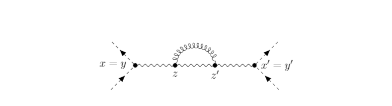
Figure 2.1: This diagram shows how the vacuum polarization contributes to the amputated 4-scalar vertex function. Dashed lines represent massive scalars, wavy lines represent photons and curly lines represent gravitons. These graphs have the same topology as Bjerrum-Bohr’s Diagram 8 [Bjerrum-Bohr:2002aqa].

Our procedure for purging gauge dependence from the one loop vacuum polarization is to write down position space representations for each of the order $e^{2}\kappa^{2}$ contributions to the amputated 4-scalar function. Any external derivatives are assumed to act on the external scalar wave functions appropriate to 2-particle scattering. By exploiting the various Donoghue Identities of Appendix LABEL:appendix:donoghue to degenerate the (internal) massive scalar propagators to Dirac delta functions, we reduce each contribution to a form that can be interpreted as a correction to $i[\mbox{}^{\mu}\Pi^{\nu}](x;x^{\prime})$.

We begin by considering the contribution of the original, gauge dependent vacuum polarization to the amputated 4-scalar function as shown in Figure 2.1. The expression for this diagram is

$$\begin{split}iV_{0}(x;x^{\prime})=&e(\partial_{x}\downarrow-\partial_{x}\uparrow)^{\alpha}\times e(\partial_{x^{\prime}}\downarrow-\partial_{x^{\prime}}\uparrow)^{\beta}\\ &\times\int d^{D}z\ i[_{\alpha}\Delta_{\mu}](x;z)\int d^{D}z^{\prime}\ i[_{\beta}\Delta_{\nu}](x^{\prime};z^{\prime})\times i[^{\mu}\Pi^{\nu}](z;z^{\prime})\end{split}$$ (2.8)

where the vacuum polarization was given in (2.3) and external derivatives with an up (down) arrow act on upper (lower) scalar wave functions at that vertex. First note that Poincaré invariance and partial integration allows us to act all longitudinal parts on the external legs, where (by current conservation) they vanish due to the on-shell condition,

$$(\partial\downarrow-\partial\uparrow)_{\mu}(\partial\downarrow+\partial\uparrow)^{\mu}=(\partial^{2}\downarrow-m^{2})-(\partial^{2}\uparrow-m^{2})\;.$$ (2.9)

We can also use the relation,

$$\frac{1}{\Delta x^{2D-2}}=\frac{\partial^{2}}{2(D\!-\!2)^{2}}\frac{1}{\Delta x^{2D-4}}=\frac{\partial^{2}}{2(D\!-\!2)^{2}}\Biggl{[}\frac{4\pi^{\frac{D}{2}}}{\Gamma(\frac{D}{2}\!-\!1)}i\Delta(x;x^{\prime})\Biggr{]}^{2}\;,$$ (2.10)

to attain the form,

$$\begin{split}iV_{0}(x;x^{\prime})=&-\frac{e^{2}\kappa^{2}\mathcal{C}_{0}(D,a,b)}{4(D\!-\!1)(D\!-\!2)}\times(\partial_{x}\downarrow-\partial_{x}\uparrow)_{\mu}(\partial_{x^{\prime}}\downarrow-\partial_{x^{\prime}}\uparrow)^{\mu}\\ &\times\int d^{D}z\ i\Delta(x;z)\int d^{D}z^{\prime}\ i\Delta(x^{\prime};z^{\prime})\,\partial_{z}^{2}\partial_{z^{\prime}}^{2}\Bigl{[}i\Delta(z;z^{\prime})\Bigr{]}^{2}\;.\end{split}$$ (2.11)

The final step is to partially integrate the factors of $\partial_{z}^{2}$ and $\partial_{z^{\prime}}^{2}$ to act on the massless propagators, and use the delta functions that result from the propagator equation (LABEL:eq:equation_massless) to eliminate the integrations over $z^{\mu}$ and ${z^{\prime}}^{\mu}$,

$$iV_{0}(x;x^{\prime})=\frac{\mathcal{C}_{0}(D,a,b)}{(D\!-\!1)(D\!-\!2)}\times\frac{e^{2}\kappa^{2}}{4}(\partial_{x}\downarrow-\partial_{x}\uparrow)\!\cdot\!(\partial_{x^{\prime}}\downarrow-\partial_{x^{\prime}}\uparrow)\times[i\Delta(x;x^{\prime})]^{2}\;.$$ (2.12)

After applying the appropriate Donoghue Identity from Appendix C it turns out that all contributions to the amputated 4-scalar function take this same form, with different gauge dependent multiplicative factors. To simplify the notation, we define a new gauge dependent constant which includes the factor of $1/(D\!-\!1)(D\!-\!2)$, and we take $D=4$ because dimensional regularization plays no role, while also dropping higher order perturbations in the gauge parameters $a=1+\delta a$ and $b=1+\delta b$,

$$\frac{\mathcal{C}_{0}(D,a,b)}{(D\!-\!1)(D\!-\!2)}\equiv C_{0}(\delta a,\delta b)+O\Bigl{(}D\!-\!4,\delta^{2}\Bigr{)}\;.$$ (2.13)

In other words, $C_{0}(\delta a,\delta b)=\frac{4}{3}+2\delta a$.

2.2.1 Correlation between Vertices

Figure 2.2: This diagram shows the contribution of graviton correlation between two vertices. Dashed lines represent massive scalars, wavy lines represent photons and curly lines represent gravitons. These graphs have the same topology as Bjerrum-Bohr’s Diagram 4 [Bjerrum-Bohr:2002aqa].

The correlation between source (at ${x^{\prime}}^{\mu}$) and observer (at $x^{\mu}$) vertices is the first extra contribution to the amputated 4-scalar function, as shown in Figure 2.2. This diagram corresponds to the analytic expression,

$$\begin{split}iV_{1}(x;x^{\prime})=&\frac{1}{2}e\kappa\left[\eta^{\delta\mu}\eta^{\nu\alpha}\!+\!\eta^{\delta\nu}\eta^{\mu\alpha}\!-\!\eta^{\mu\nu}\eta^{\delta\alpha}\right](\partial_{x}\!\uparrow\!-\partial_{x}\!\downarrow)_{\alpha}\\ &\times\frac{1}{2}e\kappa\left[\eta^{\gamma\rho}\eta^{\sigma\beta}\!+\!\eta^{\sigma\gamma}\eta^{\rho\beta}\!-\!\eta^{\rho\sigma}\eta^{\gamma\beta}\right](\partial_{x^{\prime}}\!\uparrow\!-\partial_{x^{\prime}}\!\downarrow)_{\beta}\\ &\times i[_{\mu\nu}\Delta_{\rho\sigma}](x;x^{\prime})\times i[_{\gamma}\Delta_{\delta}](x;x^{\prime})\;.\end{split}$$ (2.14)

Substituting the appropriate propagators from Appendix B, contracting all the indices, simplifying and making use of the relation,

$$i\Delta(x;x^{\prime})\frac{\partial_{\mu}\partial_{\nu}}{\partial^{2}}i\Delta(x;x^{\prime})=\frac{1}{4}\!\times\!\frac{\Gamma^{2}(\frac{D}{2}-1)}{16\pi^{D}}\left[\frac{\eta_{\mu\nu}}{\Delta x^{2D-4}}\!+\!\frac{\partial_{\mu}\partial_{\nu}}{(2D\!-\!6)}\frac{1}{\Delta x^{2D-6}}\right]\;,$$ (2.15)

gives,

$$iV_{1}(x;x^{\prime})=\frac{e^{2}\kappa^{2}\Gamma^{2}(\frac{D}{2}\!-\!1)}{16\pi^{D}}\left[D\!+\!\frac{(3D\!-\!2)\delta a}{4}\!-\!\frac{(D-2)^{2}\delta b}{4}\right](\partial_{x}\!\downarrow\!-\partial_{x}\!\uparrow)_{\mu}(\partial_{x^{\prime}}\!\downarrow\!-\partial_{x^{\prime}}\!\uparrow)_{\nu}\frac{\eta_{\mu\nu}}{\Delta x^{2D-4}}.$$ (2.16)

Note that the second term in the square bracket of expression (2.15) drops out by current conservation.

Recognizing the massless scalar propagator (LABEL:massless_scalar_prop) provides a simpler form for (2.16),

$$iV_{1}(x;x^{\prime})=\left[D\!+\!\frac{(3D\!-\!2)\delta a}{4}\!-\!\frac{(D-2)^{2}\delta b}{4}\right]\!\times\!e^{2}\kappa^{2}(\partial_{x}\!\downarrow\!-\partial_{x}\!\uparrow)\!\cdot\!(\partial_{x^{\prime}}\!\downarrow\!-\partial_{x^{\prime}}\!\uparrow)\!\times\![i\Delta(x;x^{\prime})]^{2}\;.$$ (2.17)

As promised, expression (2.16) takes the same form as the vacuum polarization contribution (2.12), but with a different gauge dependent, multiplicative constant. By comparison with (2.12) we can recognize,

$$\mathcal{C}_{1}(D,a,b)=4(D\!-\!1)(D\!-\!2)\left[D\!+\!\frac{(3D-2)\delta a}{4}\!-\!\frac{(D-2)^{2}\delta b}{4}\!+\!O(\delta^{2})\right]\;.$$ (2.18)

Henceforth we will not bother with dimensional regularization, and we will make the same notational simplification as (2.13). This means that the vertex-vertex correction is,

$$iV_{1}(x;x^{\prime})=C_{1}(\delta a,\delta b)\!\times\!\frac{e^{2}\kappa^{2}}{4}(\partial_{x}\!\downarrow\!-\partial_{x}\!\uparrow)\!\cdot\!(\partial_{x^{\prime}}\!\downarrow\!-\partial_{x^{\prime}}\!\uparrow)\!\times\![i\Delta(x;x^{\prime})]^{2}\;,$$ (2.19)

where $C_{1}(\delta a,\delta b)=16+10\delta a-4\delta b$.

2.2.2 Vertex-Force Carrier Correlations

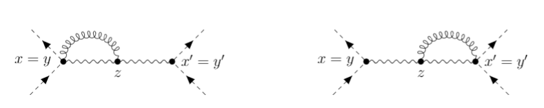
Figure 2.3: These diagrams show the contributions from correlations between the force carrier and one of the vertices. Dashed lines represent massive scalars, wavy lines represent photons and curly lines represent gravitons. These graphs have the same topology as Bjerrum-Bohr’s Diagram 7 [Bjerrum-Bohr:2002aqa].

The next contribution comes from the correlations between a single vertex and the exchange photon, as shown in Figure 2.3. The analytic form is,

$$\begin{split}iV_{2}(x;x^{\prime})=&\frac{1}{2}e\kappa\left[\eta^{\epsilon\mu}\eta^{\nu\beta}+\eta^{\epsilon\nu}\eta^{\mu\beta}-\eta^{\mu\nu}\eta^{\epsilon\beta}\right](\partial_{x}\uparrow-\partial_{x}\downarrow)_{\beta}\times e(\partial_{x^{\prime}}\downarrow-\partial_{x^{\prime}}\uparrow)^{\theta}\\ &\times\int d^{D}z\ (-i\kappa V^{\gamma\delta\alpha\tau\rho\sigma})\ \partial_{z\tau}i[_{\epsilon}\Delta_{\delta}](x;z)\ \partial_{z\alpha}i[_{\gamma}\Delta_{\theta}](z;x^{\prime})\times i[_{\mu\nu}\Delta_{\rho\sigma}](x;z)\\ &+(\text{Permutation})\;.\end{split}$$ (2.20)

For reducing this diagram it is useful to note how the product of a massless propagator times one of the gauge variations can be expressed as a differential operator acting on a single function of the Poincaré interval,

$$i\Delta(x;x^{\prime})\frac{\partial_{\mu}\partial_{\nu}}{\partial^{2}}i\Delta(x;x^{\prime})= \frac{1}{4}\eta_{\mu\nu}[i\Delta(x;x^{\prime})]^{2}-\frac{1}{8}\partial_{\mu}\partial_{\nu}I\{[i\Delta(x;x^{\prime})]^{2}\}\;,$$ (2.21)

$$\begin{split}\partial_{\kappa}i\Delta(x;x^{\prime})\frac{\partial_{\alpha}\partial_{\beta}}{\partial^{2}}i\Delta(x;x^{\prime})&=\frac{D-2}{16(D-1)}\partial_{\kappa}\partial_{\alpha}\partial_{\beta}I\{[i\Delta(x;x^{\prime})]^{2}\}+\frac{D}{8(D-1)}\eta_{\alpha\beta}\partial_{\kappa}[i\Delta(x;x^{\prime})]^{2}\\ &-\frac{D-2}{8(D-1)}(\eta_{\kappa\alpha}\partial_{\beta}+\eta_{\kappa\beta}\partial_{\alpha})[i\Delta(x;x^{\prime})]^{2}\;,\end{split}$$ (2.22)

where the symbol $I\{\}$ represents indefinite integration of the argument with respect to $\Delta x^{2}$. The final result for these diagrams is,

$$iV_{2}(x;x^{\prime})=C_{2}(\delta a,\delta b)\!\times\!\frac{e^{2}\kappa^{2}}{4}(\partial_{x}\!\downarrow\!-\partial_{x}\!\uparrow)\!\cdot\!(\partial_{x^{\prime}}\!\downarrow\!-\partial_{x^{\prime}}\!\uparrow)\!\times\![i\Delta(x;x^{\prime})]^{2}\;,$$ (2.23)

where $C_{2}(\delta a,\delta b)=-12-16\delta a+4\delta b$.

2.2.3 Vertex-Source and Vertex-Observer Correlations

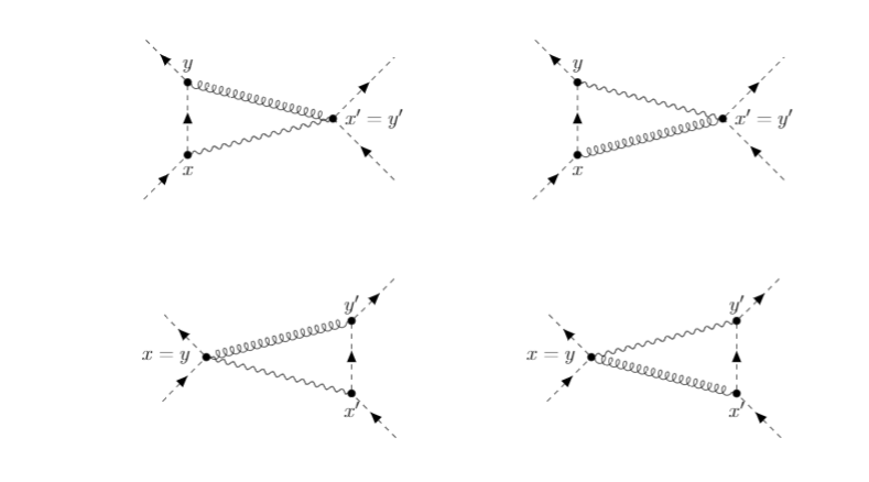
Figure 2.4: These diagrams show the contributions from correlations between the source (primed) or observer (unprimed) and the opposite vertex. Dashed lines represent massive scalars, wavy lines represent photons and curly lines represent gravitons. These graphs have the same topology as Bjerrum-Bohr’s Diagram 3 [Bjerrum-Bohr:2002aqa].

We next consider contribution from correlations between the source, or observer, and the opposite vertex, as shown in Figure 2.4. (Correlations with nearer vertices do not contribute because they are cancelled by field strength renormalization.) We use $x^{\mu}$ ($y^{\mu}$) for incoming (outgoing) observer, and ${x^{\prime}}^{\mu}$ (${y^{\prime}}^{\mu}$) for incoming (outgoing) source. We also adopt the notation that a bar over a vertex with only a single external leg denotes differentiation of the on-shell external wave function. With these conventions we can write the analytic form of the diagrams in Figure 2.4 as,

$$\begin{split}{\rm Figure\ \ref{fig:triangular}}=&\frac{i\kappa}{2}\left[\bar{\partial}^{\mu}_{y}\partial^{\nu}_{y}\!+\!\bar{\partial}^{\nu}_{y}\partial^{\mu}_{y}\!-\!\eta^{\mu\nu}\left(\partial_{y}\!\cdot\!\bar{\partial}_{y}\!+\!m^{2}\right)\right]\!\times\!e(\bar{\partial}_{x}\!-\!\partial_{x})^{\delta}i\Delta_{m}(x;y)\\ &\times\frac{e\kappa}{2}\left[\eta^{\gamma\rho}\eta^{\alpha\sigma}\!+\!\eta^{\gamma\sigma}\eta^{\alpha\rho}\!-\!\eta^{\rho\sigma}\eta^{\alpha\gamma}\right](\partial_{x^{\prime}}\!\uparrow\!-\partial_{x^{\prime}}\!\downarrow)_{\alpha}\!\times\!i[_{\delta}\Delta_{\gamma}](x;x^{\prime})\!\times\!i[_{\mu\nu}\Delta_{\rho\sigma}](y;x^{\prime})\\ &+(3\ \text{permutations})\;.\end{split}$$ (2.24)

As can be seen from Figure 2.4, these contributions involve an internal massive scalar propagator in the loop. This poses an obstacle to regarding expression (2.24) as a correction to the vacuum polarization. This is overcome through the “Donoghue Identities” of Appendix LABEL:appendix:donoghue, which degenerate the massive scalar propagator to a Dirac delta function, and reduce expression (2.24) to the same 2-point form (2.12) as the contribution from the original vacuum polarization. The part of expression (2.24) which is independent of the gauge parameters $\delta a$ and $\delta b$ reaches the desired form through the Donoghue Identities (LABEL:eq:3pt) and (LABEL:eq:3pt_derivative).

As an example of the part of (2.24) proportional to $\delta a$, we consider the term,

$$\begin{split}\delta a&\times\frac{i\kappa}{2}\left[\bar{\partial}^{\mu}_{y}\partial^{\nu}_{y}\!+\!\bar{\partial}^{\nu}_{y}\partial^{\mu}_{y}\!-\!\eta^{\mu\nu}\left(\partial_{y}\!\cdot\!\bar{\partial}_{y}\!+\!m^{2}\right)\right]\!\times\!e(\bar{\partial}_{x}\!-\!\partial_{x})^{\delta}i\Delta_{m}(x;y)\\ &\times\frac{e\kappa}{2}\left[\eta^{\gamma\rho}\eta^{\alpha\sigma}\!+\!\eta^{\gamma\sigma}\eta^{\alpha\rho}\!-\!\eta^{\rho\sigma}\eta^{\alpha\gamma}\right](\partial_{x^{\prime}}\!\uparrow\!-\partial_{x^{\prime}}\!\downarrow)_{\alpha}\!\times\!i[_{\delta}\Delta_{\gamma}](x;x^{\prime})\!\times\!\eta_{\nu\rho}\frac{\partial_{\mu}\partial_{\sigma}}{\partial^{2}}i\Delta(y;x^{\prime})\;.\end{split}$$ (2.25)

The derivative $\partial_{\mu}$ acting on the massless propagator $i\Delta(y;x^{\prime})$ can be partially integrated to act on the massive propagator $i\Delta_{m}(x;y)$,

$$-(\bar{\partial}_{y}\!+\!\partial_{y})_{\mu}\left[\bar{\partial}^{\mu}_{y}\partial^{\nu}_{y}\!+\!\bar{\partial}^{\nu}_{y}\partial^{\mu}_{y}\!-\!\eta^{\mu\nu}\left(\partial_{y}\!\cdot\!\bar{\partial}_{y}\!+\!m^{2}\right)\right]=-\bar{\partial}_{y}^{\nu}i\delta^{D}(x\!-\!y)\;.$$ (2.26)

The remaining factor of $\partial^{\sigma}/\partial^{2}$ can be reduced using,

$$i\Delta(x;x^{\prime})\!\times\!\frac{\partial_{\alpha}}{\partial^{2}}i\Delta(x;x^{\prime})=\frac{1}{4}\partial_{\alpha}I\{[i\Delta(x;x^{\prime})]^{2}\}\;,$$ (2.27)

$$\partial^{2}I\{[i\Delta(x;x^{\prime})]^{2}\}\longrightarrow-2(D\!-\!4)[i\Delta(x;x^{\prime})]^{2}\;.$$ (2.28)

From expression (LABEL:eq:graviton_prop) for the graviton propagator we see that there are two parts proportional to $\delta b$. The second term with $\partial_{\mu}\partial_{\nu}/\partial^{2}$ can be reduced just like (2.25). The other term requires additional effort,

$$\begin{split}-2\delta b&\times\frac{i\kappa}{2}\left[\bar{\partial}^{\mu}_{y}\partial^{\nu}_{y}\!+\!\bar{\partial}^{\nu}_{y}\partial^{\mu}_{y}\!-\!\eta^{\mu\nu}\left(\partial_{y}\!\cdot\!\bar{\partial}_{y}\!+\!m^{2}\right)\right]\!\times\!e(\bar{\partial}_{x}\!-\!\partial_{x})^{\delta}i\Delta_{m}(x;y)\\ &\times\frac{e\kappa}{2}\left[\eta^{\gamma\rho}\eta^{\alpha\sigma}\!+\!\eta^{\gamma\sigma}\eta^{\alpha\rho}\!-\!\eta^{\rho\sigma}\eta^{\alpha\gamma}\right](\partial_{x^{\prime}}\!\uparrow\!-\partial_{x^{\prime}}\!\downarrow)_{\alpha}\!\times\!i[_{\delta}\Delta_{\gamma}](x;x^{\prime})\!\times\!\eta_{\mu\nu}\frac{\partial_{\rho}\partial_{\sigma}}{\partial^{2}}i\Delta(y;x^{\prime})\;.\end{split}$$ (2.29)

To reduce this term we distinguish between $y^{\mu}$ derivatives acting on the external leg ($\bar{\partial}_{y}^{\mu}$), the massive propagator ($\partial_{y}^{\mu}$) and the massless propagator of the graviton ($\tilde{\partial}_{y}^{\mu}$),

$$\bar{\partial}_{y}^{\mu}+\partial_{y}^{\mu}+\tilde{\partial}_{y}^{\mu}=0\;.$$ (2.30)

Now note that,

$$\eta_{\mu\nu}\left[\bar{\partial}^{\mu}_{y}\partial^{\nu}_{y}\!+\!\bar{\partial}^{\nu}_{y}\partial^{\mu}_{y}\!-\!\eta^{\mu\nu}\left(\partial_{y}\!\cdot\!\bar{\partial}_{y}\!+\!m^{2}\right)\right]=(\bar{\partial}_{y}^{2}\!-\!m^{2})+(\partial_{y}^{2}\!-\!m^{2})-\tilde{\partial}_{y}^{2}-2m^{2}\;.$$ (2.31)

The factor of $(\bar{\partial}_{y}^{2}-m^{2})$ vanishes due to the external leg being on shell. The next term in (2.31) degenerates the massive scalar propagator,

$$(\partial_{y}^{2}\!-\!m^{2})i\Delta_{m}(x;y)=i\delta^{D}(x\!-\!y)\;.$$ (2.32)

Of course the factor of $\tilde{\partial}_{y}^{2}$ eliminates the troublesome inverse D‘Alembertian, whereupon the Donoghue Identity (LABEL:eq:3pt_2derivative) completes the reduction. The final term in (2.31) requires the newly Donoghue Identities (LABEL:eq:new_dono_1) and (LABEL:eq:new_dono_2).

Putting everything together gives the final result for Figure 2.4,

$$iV_{3}(x;x^{\prime})=C_{3}(\delta a,\delta b)\!\times\!\frac{e^{2}\kappa^{2}}{4}(\partial_{x}\!\downarrow\!-\partial_{x}\!\uparrow)\!\cdot\!(\partial_{x^{\prime}}\!\downarrow\!-\partial_{x^{\prime}}\!\uparrow)\!\times\![i\Delta(x;x^{\prime})]^{2}\;,$$ (2.33)

where $C_{3}(\delta a,\delta b)=-32-8\delta a-2\delta b$.

2.2.4 Source-Observer Correlations

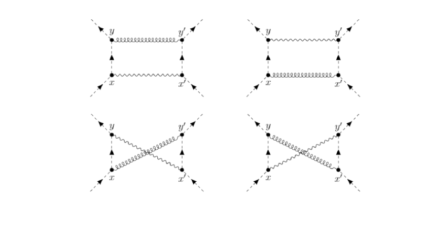
Figure 2.5: These diagrams show the contributions from correlations between the source (primed) and observer (unprimed). Dashed lines represent massive scalars, wavy lines represent photons and curly lines represent gravitons. These graphs have the same topology as Bjerrum-Bohr’s Diagram 2 [Bjerrum-Bohr:2002aqa].

Figure 2.5 shows contributions from correlations between source and observer. (Correlations between the source and itself, or the observer and itself, do not correct the exchange photon.) The analytic form for these diagrams is,

$$\begin{split}(\rm Figure\ \ref{fig:box})=&\frac{i\kappa}{2}\left[\bar{\partial}_{y}^{\mu}\partial_{y}^{\nu}\!+\!\bar{\partial}_{y}^{\nu}\partial_{y}^{\mu}\!-\!\eta^{\mu\nu}\left(\bar{\partial}_{y}\!\cdot\!\partial_{y}\!+\!m^{2}\right)\right]\left(\bar{\partial}_{x}\!-\!\partial_{x}\right)^{\delta}i\Delta_{m}(x;y)\\ &\times\frac{i\kappa}{2}\left[\bar{\partial}_{y^{\prime}}^{\rho}\partial_{y^{\prime}}^{\sigma}\!+\!\bar{\partial}_{y^{\prime}}^{\sigma}\partial_{y^{\prime}}^{\rho}\!-\!\eta^{\rho\sigma}\left(\bar{\partial}_{y^{\prime}}\!\cdot\!\partial_{y^{\prime}}\!+\!m^{2}\right)\right]\left(\bar{\partial}_{x^{\prime}}\!-\!\partial_{x^{\prime}}\right)^{\gamma}i\Delta_{m}(x^{\prime};y^{\prime})\\ &\times i[_{\gamma}\Delta_{\delta}](x;x^{\prime})\!\times\!i[_{\mu\nu}\Delta_{\rho\sigma}](y;y^{\prime})+(3\text{ Permutations})\;.\end{split}$$ (2.34)

Note that the two permutations on the bottom line of Figure 2.5 contain an extra minus sign due to 2-scalar-1-photon vertex.

The part of (2.34) independent of $\delta a$ and $\delta b$ is accomplished by the Donoghue Identity (LABEL:eq:box_dono). The reduction of the gauge dependent parts is similar to what we have seen before with one difference: after using relation (2.26), one must combine parts from the various diagrams to eliminate some troublesome terms. The final result for Figure 2.5 is,

$$iV_{4}(x;x^{\prime})=C_{4}(\delta a,\delta b)\!\times\!\frac{e^{2}\kappa^{2}}{4}(\partial_{x}\!\downarrow\!-\partial_{x}\!\uparrow)\!\cdot\!(\partial_{x^{\prime}}\!\downarrow\!-\partial_{x^{\prime}}\!\uparrow)\!\times\![i\Delta(x;x^{\prime})]^{2}\;,$$ (2.35)

where $C_{4}(\delta a,\delta b)=\frac{80}{3}+0\cdot\delta a+2\delta b$.

2.2.5 Force Carrier Correlations with Source and Observer

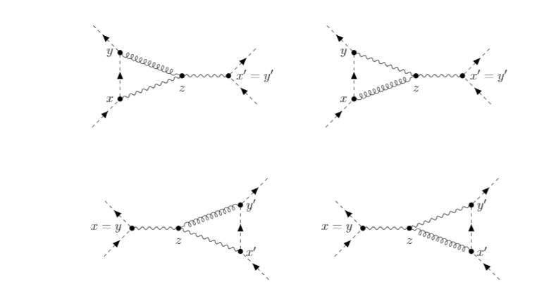
Figure 2.6: These diagrams show the contributions from correlations between the source (primed) or observer (unprimed) and the force carrier. Dashed lines represent massive scalars, wavy lines represent photons and curly lines represent gravitons. These graphs have the same topology as Bjerrum-Bohr’s Diagram 6 [Bjerrum-Bohr:2002aqa].

The next contribution comes from correlations between the source or observer and the photon. The Feynman diagrams are given in Figure 2.6, and the analytic expression is,

$$\begin{split}{\rm(Figure\ \ref{fig:force_source_obs})}=&\frac{i\kappa}{2}\left[\bar{\partial}_{y}^{\mu}\partial_{y}^{\nu}\!+\!\bar{\partial}_{y}^{\nu}\partial_{y}^{\mu}\!-\!\eta^{\mu\nu}\left(\bar{\partial}_{y}\!\cdot\!\partial_{y}\!+\!m^{2}\right)\right]\left(\bar{\partial}_{x}\!-\!\partial_{x}\right)^{\epsilon}i\Delta_{m}(x;y)\\ &\times\int\!\!d^{D}z(-i\kappa V^{\gamma\delta\alpha\tau\rho\sigma})\frac{\partial}{\partial z^{\tau}}i[_{\epsilon}\Delta_{\delta}](x;z)\frac{\partial}{\partial z^{\alpha}}i[_{\gamma}\Delta_{\theta}](z;x^{\prime})\!\times\!e\left(\partial_{x^{\prime}}\!\downarrow\!-\partial_{x^{\prime}}\!\uparrow\right)^{\theta}\\ &\times i[_{\mu\nu}\Delta_{\rho\sigma}]+(3\text{ Permutations})\;.\end{split}$$ (2.36)

The reduction process is almost same as in Section 2.2.3, the chief difference being the extra photon propagator. We extract a D’Alembertian and then use (LABEL:eq:equation_massless) to eliminate this and the integration over $z^{\mu}$. The final contribution from these diagrams is,

$$iV_{5}(x;x^{\prime})=C_{5}(\delta a,\delta b)\!\times\!\frac{e^{2}\kappa^{2}}{4}(\partial_{x}\!\downarrow\!-\partial_{x}\!\uparrow)\!\cdot\!(\partial_{x^{\prime}}\!\downarrow\!-\partial_{x^{\prime}}\!\uparrow)\!\times\![i\Delta(x;x^{\prime})]^{2}\;,$$ (2.37)

where $C_{5}(\delta a,\delta b)=12+12\delta a+4\delta b$.

2.2.6 Gravitational 1-PR Vertex Corrections

The final contribution to the amputated 4-scalar function comes from diagrams in which a loop of photons corrects one of the vertices and the graviton carries the exchange force. The relevant diagrams are shown in Figure 2.7.

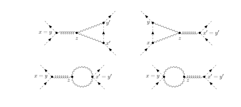
Figure 2.7: These diagrams show the contributions from the 1PR (one particle reducible) diagrams corresponding to gravitational vertex corrections. Dashed lines represent massive scalars, wavy lines represent photons and curly lines represent gravitons. These graphs have the same topology as Bjerrum-Bohr’s Diagram 5 [Bjerrum-Bohr:2002aqa].

The analytic form for first two diagrams is,

$$\begin{split}\text{Figure 6}_{\text{up}}=&\frac{i\kappa}{2}\left[\partial_{x}^{\mu}\!\uparrow\partial_{x}^{\nu}\!\downarrow\!+\!\partial_{x}^{\nu}\!\uparrow\partial_{x}^{\mu}\!\downarrow\!-\!\eta^{\mu\nu}\left(\partial_{x}\!\uparrow\!\cdot\!\partial_{x}\!\downarrow\!+\!m^{2}\right)\right]\!\times\!e\left(\bar{\partial}_{x^{\prime}}\!-\!\partial_{x^{\prime}}\right)^{\theta}\\ &\times e\left(\partial_{y^{\prime}}\!-\!\bar{\partial}_{y^{\prime}}\right)^{\epsilon}i\Delta_{m}(x^{\prime};y^{\prime})\int\!\!d^{D}z\ (-i\kappa V^{\gamma\delta\alpha\tau\rho\sigma})\frac{\partial}{\partial z^{\tau}}i[_{\epsilon}\Delta_{\delta}](z;x^{\prime})\frac{\partial}{\partial z^{\alpha}}i[_{\gamma}\Delta_{\theta}](z;x^{\prime})\\ &\times i[_{\mu\nu}\Delta_{\rho\sigma}](x;z)+(\text{Permutation})\;.\end{split}$$ (2.38)

The second two diagrams are,

$$\begin{split}\text{Figure 6}_{\text{down}}=&\frac{1}{2}\!\times\!\frac{i\kappa}{2}\left[\partial_{x}^{\mu}\!\uparrow\partial_{x}^{\nu}\!\downarrow\!+\!\partial_{x}^{\nu}\!\uparrow\partial_{x}^{\mu}\!\downarrow\!-\!\eta^{\mu\nu}\left(\partial_{x}\!\uparrow\!\cdot\!\partial_{x}\!\downarrow\!+\!m^{2}\right)\right]\!\times\!(-2ie^{2}\eta^{\epsilon\theta})\\ &\int\!\!d^{D}z(-i\kappa V^{\gamma\delta\alpha\tau\rho\sigma})\frac{\partial}{\partial z^{\tau}}i[_{\epsilon}\Delta_{\delta}](z;y^{\prime})\frac{\partial}{\partial z^{\alpha}}i[_{\gamma}\Delta_{\theta}](z;x^{\prime})\\ &\times i[_{\mu\nu}\Delta_{\rho\sigma}](x;z)+(\text{Permutation})\;.\end{split}$$ (2.39)

Whenever possible, it is prudent to partially integrate and reflect a derivative through the graviton propagator to act on the 2-scalar-1-graviton vertex. One then makes use of the relation,

$$(\partial_{x}\!\downarrow\!+\!\partial_{x}\!\uparrow)_{\mu}\left[\partial_{x}^{\mu}\!\uparrow\partial_{x}^{\nu}\!\downarrow\!+\!\partial_{x}^{\nu}\!\uparrow\partial_{x}^{\mu}\!\downarrow\!-\!\eta^{\mu\nu}\left(\partial_{x}\!\uparrow\!\cdot\!\partial_{x}\!\downarrow\!+\!m^{2}\right)\right]=0\;.$$ (2.40)

The rest of the reduction is same as in earlier sections. The final result is,

$$iV_{6}(x;x^{\prime})=C_{6}(\delta a,\delta b)\!\times\!\frac{e^{2}\kappa^{2}}{4}(\partial_{x}\!\downarrow\!-\partial_{x}\!\uparrow)\!\cdot\!(\partial_{x^{\prime}}\!\downarrow\!-\partial_{x^{\prime}}\!\uparrow)\!\times\![i\Delta(x;x^{\prime})]^{2}\;,$$ (2.41)

where $C_{6}(\delta a,\delta b)=-\frac{16}{3}+0\cdot\delta a-4\delta b$.

2.2.7 Sum Total

As we have explained, the Donoghue Identities of Appendix LABEL:appendix:donoghue allow us to cast each contribution to the amputated 4-scalar function in the form,

$$iV_{i}(x;x^{\prime})=C_{i}(\delta a,\delta b)\!\times\!\frac{e^{2}\kappa^{2}}{4}(\partial_{x}\!\downarrow\!-\partial_{x}\!\uparrow)\!\cdot\!(\partial_{x^{\prime}}\!\downarrow\!-\partial_{x^{\prime}}\!\uparrow)\!\times\![i\Delta(x;x^{\prime})]^{2}\;,$$ (2.42)

where the gauge dependent constant is $C_{i}(\delta a,\delta b)=O_{i}+A_{i}\delta a+B_{i}\delta b$. Table 2.1 summarizes our results.

Table 2.1: The entry on the $i^{\text{th}}$ row represent the gauge dependent factors for the contribution coming from the diagram in Figure $i+1$.

$i$	Description	$\quad O_{i}\quad$	$\quad A_{i}\quad$	$\quad B_{i}\quad$
0	Vacuum Polarization	$+\frac{4}{3}$	$+2$	$0$
1	Circular Diagram	$+16$	$+10$	$-4$
2	Vertex-Force Carrier	$-12$	$-16$	$+4$
3	Triangular Diagrams	$-32$	$-8$	$-2$
4	Box Diagrams	$+\frac{80}{3}$	$0$	$+2$
5	Source, Obs.- Force Carrier	$+12$	$+12$	$+4$
6	Graviton 1PR Vertex	$-\frac{16}{3}$	$0$	$-4$
	Total	$+\frac{20}{3}$	$0$	$0$

Of course the point of the exercise is to total the $O_{i}$’s, and to show that the terms proportional to $\delta a$ and $\delta b$ sum to zero,

$$\sum_{i=0}^{6}iV_{i}(x;x^{\prime})=+\frac{20}{3}\times\frac{e^{2}\kappa^{2}}{4}(\partial_{x}\!\downarrow\!-\partial_{x}\!\uparrow)\!\cdot\!(\partial_{x^{\prime}}\!\downarrow\!-\partial_{x^{\prime}}\!\uparrow)\!\times\![i\Delta(x;x^{\prime})]^{2}\;.$$ (2.43)

We then reverse the steps that led from expression (2.8) to (2.12) in order to conclude that the gauge independent vacuum polarization from a single graviton loop is,

$$i[^{\mu}\Pi^{\nu}](x;x^{\prime})=-\frac{40}{3}\!\times\!\frac{\kappa^{2}}{16\pi^{4}}\left[\eta^{\mu\nu}\partial^{2}\!-\!\partial^{\mu}\partial^{\nu}\right]\frac{1}{\Delta x^{2D-2}}\;.$$ (2.44)

2.3 Conclusions

The main result of this chapter is that including quantum gravitational corrections from the source which disturbs the effective field, and from the observer who measures the disturbance, eliminates the massive gauge dependence of the quantum-corrected Maxwell equation (2.1) that was evident in the multiplicative constant $\mathcal{C}_{0}(D,a,b)$ of expression (2.4). After renormalization, and application of the Schwinger-Keldysh formalism [Ford:2004wc], our final result for the one loop effective field equation is,

$$\partial_{\nu}F^{\nu\mu}(x)+\frac{5\hbar G\partial^{6}}{48\pi^{2}c^{3}}\!\int\!\!d^{4}x^{\prime}\,\theta(\Delta t\!-\!\Delta r)\Bigl{\{}\ln[\mu^{2}(\Delta t^{2}\!-\!r^{2})]\!-\!1\Bigr{\}}\partial_{\nu}^{\prime}F^{\nu\mu}(x^{\prime})=J^{\mu}(x)\;,$$ (2.45)

where $\Delta t\equiv t-t^{\prime}$, $r\equiv\|\vec{x}-\vec{x}^{\prime}\|$ and we have restored the factors $\hbar$ and $c$. Although equation (2.45) is not local, it is real and causal.

For a static point charge $J^{\mu}(t,\vec{x})=q\delta^{\mu}_{~{}0}\delta^{3}(\vec{x}\!-\!\vec{x}^{\prime})$ the quantum-corrected Coulomb potential is,

$$\Phi(r)=\frac{q}{4\pi r}\left\{1+\frac{10\hbar G}{3\pi r^{2}c^{3}}+\mathcal{O}(G^{2})\right\}.$$ (2.46)

This result agreees with Bjerrum-Bohr [Bjerrum-Bohr:2002aqa], but we now have the ability to solve for quantum gravitational corrections to the full range of problems one encounters in classical electrodynamics. These corrections are bound to be quite small under ordinary conditions, although the potential for slightly super-luminal propagation is noteworthy [Leonard:2012fs], and was predicted long ago [Deser:1957zz, DeWitt:1960fc].

Although it is nice to finally be able to include quantum gravitational corrections to Maxwell’s equations on flat space background, we could always have inferred physics from scattering amplitudes. The real necessity for our method is for studying quantum gravitational corrections to electrodynamics in cosmology. These effects can be significant, especially during the epoch of primordial inflation. For example, when the simplest de Sitter background gauge [Tsamis:1992xa, Woodard:2004ut] is employed to compute single graviton loop corrections to the vacuum polarization [Leonard:2013xsa] one finds corrections to the Coulomb potential [Glavan:2013jca], and to the photon field strength [Wang:2014tza] which become nonperturbatively strong at large distances and late times. When the vacuum polarization is computed in a much more complicated, 1-parameter family of gauges [Glavan:2015ura], one finds the same time dependence for the photon field strength, but with a different numerical coefficient [Glavan:2016bvp], signaling a slight gauge dependence which must be eliminated to infer reliable results. First order corrections to the graviton propagator in the de Sitter generalization of the gauge (2.2) have been derived recently [Glavan:2019msf]. This should facilitate extending the current work to de Sitter background.

Chapter 3 Perturbative Quantum Gravity Induced Scalar Coupling to Electromagnetism

3.1 Introduction

There has been much recent interest in searching for exotic processes which might be induced by quantum gravity [Piscicchia:2022xra, Piscicchia:2022eod]. In particular, it has been suggested [Calmet:2022bin] that quantum gravitationally induced scalar couplings to electromagnetism might be detected by planned atom interferometers such as MAGIS [Abe:2021magis], AION [Badurina:2019hst, Badurina:2021rgt] and AEDGE [AEDGE:2019nxb]. Conventional wisdom has it that perturbative quantum gravity can at best generate couplings of dimension eight, and that couplings of dimensions 5 and 6 could only be induced, with unknown coefficients, by nonperturbative effects [Calmet:2019frv] such as gravitational instantons [Perry:1978fd, Chen:2021jcb] and wormholes [Gilbert:1989nq].

In this chapter we point out that there is a completely perturbative mechanism through which quantum gravity induces a dimension six coupling of a massive scalar with a precisely calculable coefficient. The mechanism is simple: assuming that the scalar is constant in space and time, and that the potential energy from its mass dominates the stress-energy, the background geometry will be de Sitter with a Hubble parameter which depends in a precise way on the scalar. Unlike the graviton propagator in flat space, the coincidence limit of a graviton propagator on de Sitter background goes like the square of the Hubble parameter in any gauge [Tsamis:1992xa, Woodard:2004ut, Miao:2011fc, Mora:2012zi, Glavan:2019msf]. Hence integrating out pairs of graviton fields from the Heisenberg operator Maxwell equation (the Hartree approximation) induces couplings of the desired form with precisely computable coefficients.

This short chapter contains only three sections, of which this Introduction is the first. We present the calculation in Section 3.2. Our conclusions comprise Section 3.3.

3.2 Calculation

Consider a massive, uncharged scalar field which is coupled to electromagnetism and gravity,

$$\mathcal{L}=-\frac{1}{2}\partial_{\mu}\varphi\partial_{\nu}\varphi g^{\mu\nu}\sqrt{-g}-\frac{1}{2}m^{2}\varphi^{2}\sqrt{-g}-\frac{1}{4}F_{\mu\nu}F_{\rho\sigma}g^{\mu\rho}g^{\nu\sigma}\sqrt{-g}-\frac{R\sqrt{-g}}{16\pi G}\;.$$ (3.1)

The corresponding Einstein equation is

$$G_{\mu\nu}=8\pi G\left[\partial_{\mu}\varphi\partial_{\nu}\varphi-\frac{1}{2}g_{\mu\nu}g^{\rho\sigma}\partial_{\rho}\varphi\partial_{\sigma}\varphi-\frac{1}{2}m^{2}\varphi^{2}g_{\mu\nu}+F_{\mu\rho}F_{\nu\sigma}g^{\rho\sigma}-\frac{1}{4}g_{\mu\nu}g^{\alpha\beta}g^{\rho\sigma}F_{\alpha\rho}F_{\beta\sigma}\right].$$ (3.2)

As discussed in the introduction, we assume that $\varphi=\varphi_{0}$ is a constant and also set $A_{\mu}=0$ to get,

$$G_{\mu\nu}=8\pi G\times-\frac{1}{2}m^{2}\varphi_{0}^{2}g_{\mu\nu}\;.$$ (3.3)

The unique, maximally symmetric solution is de Sitter with Hubble constant,

$$H=\sqrt{\frac{4\pi G}{3}\times m^{2}\varphi_{0}^{2}}\;.$$ (3.4)

where, $H$ is the Hubble constant. This shows that a constant scalar triggers a phase of de Sitter inflation. Because de Sitter is conformally flat, there is no classical effect on electromagnetism in conformal coordinates. However, we will see that the breaking of conformal invariance by gravity does induce a quantum effect.

Consider the Maxwell equation in a general metric $g_{\mu\nu}$,

$$\partial_{\nu}\Bigl{[}\sqrt{-g}\,g^{\mu\rho}g^{\nu\sigma}F_{\sigma\rho}\Bigr{]}=J^{\mu}\;,$$ (3.5)

where $F_{\mu\nu}\equiv\partial_{\mu}A_{\nu}-\partial_{\nu}A_{\mu}$ is the field strength tensor and $J^{\mu}$ is the current density. We write the quantum metric $g_{\mu\nu}$ in terms of the Minkowski metric $\eta_{\mu\nu}$,

$$g_{\mu\nu}\equiv a^{2}\tilde{g}_{\mu\nu}=a^{2}\Bigl{[}\eta_{\mu\nu}+\kappa h_{\mu\nu}\Bigr{]}\;,$$ (3.6)

where $\kappa^{2}\equiv 16\pi G$ is the loop counting parameter, $a(\eta)\equiv-1/H\eta$ is the scale factor at conformal time $\eta$ and $h_{\mu\nu}$ is the graviton field. Graviton indices are raised and lowered with the Minkowski metric: $h^{\mu}_{~{}\nu}\equiv\eta^{\mu\rho}h_{\rho\nu}$, $h^{\mu\nu}\equiv\eta^{\mu\rho}\eta^{\nu\sigma}h_{\rho\sigma}$. The inverse and determinant of the conformally transformed metric are,

$$\tilde{g}^{\alpha\beta} = \eta^{\alpha\beta}-\kappa h^{\alpha\beta}+\kappa^{2}h^{\alpha\rho}h^{\beta}_{~{}\rho}-\cdots\;,$$ (3.7)

$$\sqrt{-\tilde{g}} = 1+\frac{1}{2}\kappa h+\kappa^{2}\left(\frac{1}{8}h^{2}-\frac{1}{4}h^{\rho\sigma}h_{\rho\sigma}\right)+\cdots$$ (3.8)

Here $h$ is the trace of the graviton field $h\equiv\eta^{\mu\nu}h_{\mu\nu}$.

To facilitate dimensional regularization we formulate the theory in $D$ spacetime dimensions. The term inside the square bracket of equation (3.5) can be expressed in terms of the conformally transformed metric as $\sqrt{-g}\,g^{\mu\rho}g^{\nu\sigma}F_{\sigma\rho}\equiv a^{D-4}\sqrt{-\tilde{g}}\,\tilde{g}^{\mu\rho}\tilde{g}^{\nu\sigma}F_{\sigma\rho}$. The terms involving $\tilde{g}_{\mu\nu}$ can be expanded as,

$$\tilde{g}^{\mu\rho}\tilde{g}^{\nu\sigma}\sqrt{-\tilde{g}}=\eta^{\mu\rho}\eta^{\nu\sigma}+\kappa\Bigl{[}\frac{1}{2}h\eta^{\mu\rho}\eta^{\nu\sigma}-h^{\mu\rho}\eta^{\nu\sigma}-\eta^{\mu\rho}h^{\nu\sigma}\Bigr{]}+\kappa^{2}\Biggl{[}\Bigl{(}\frac{1}{8}h^{2}\!-\!\frac{1}{4}h^{\alpha\beta}h_{\alpha\beta}\Bigr{)}\eta^{\mu\rho}\eta^{\nu\sigma}$$ (3.9)

$$\hskip 85.35826pt-\frac{1}{2}hh^{\mu\rho}\eta^{\nu\sigma}\!-\!\frac{1}{2}h\eta^{\mu\rho}h^{\nu\sigma}\!+\!h^{\mu\alpha}h^{\rho}_{~{}\alpha}\eta^{\nu\sigma}\!+\!\eta^{\mu\rho}h^{\nu\alpha}h^{\sigma}_{~{}\alpha}\!+\!h^{\mu\rho}h^{\nu\sigma}\Biggr{]}\!+\!\mathcal{O}(\kappa^{3})\;.\qquad$$

Using the Hartree approximation [Hartree:1928, Mora:2013ypa], we can replace the terms proportional to $\kappa$ by zero and the terms proportional to $\kappa^{2}$ by the coincidence limit of the graviton propagator $i[\mbox{}_{\mu\nu}\Delta_{\rho\sigma}](x;x^{\prime})$,

$$\tilde{g}^{\mu\rho}\tilde{g}^{\nu\sigma}\sqrt{-\tilde{g}}\longrightarrow\eta^{\mu\rho}\eta^{\nu\sigma}+\kappa^{2}\Biggl{[}\Bigl{(}\frac{1}{8}i\Bigl{[}\mbox{}^{\alpha}_{~{}\alpha}\Delta^{\beta}_{~{}\beta}\Bigr{]}-\frac{1}{4}i\Bigl{[}\mbox{}^{\alpha\beta}\Delta_{\alpha\beta}\Bigr{]}\Bigr{)}\eta^{\mu\rho}\eta^{\nu\sigma}-\frac{1}{2}i\Bigl{[}\mbox{}^{\alpha}_{~{}\alpha}\Delta^{\mu\rho}\Bigr{]}\eta^{\nu\sigma}$$ (3.10)

$$\hskip 71.13188pt-\frac{1}{2}i\Bigl{[}\mbox{}^{\alpha}_{~{}\alpha}\Delta^{\nu\sigma}\Bigr{]}\eta^{\mu\rho}+i\Bigl{[}\mbox{}^{\mu\alpha}\Delta^{\rho}_{~{}\alpha}\Bigr{]}\eta^{\nu\sigma}+\eta^{\mu\rho}i\Bigl{[}\mbox{}^{\nu\alpha}\Delta^{\sigma}_{~{}\alpha}\Bigr{]}+i\Bigl{[}\mbox{}^{\mu\rho}\Delta^{\nu\sigma}\Bigr{]}\Biggr{]}+\mathcal{O}(\kappa^{4})\;.\qquad$$

The graviton is of course gauge dependent but its coincidence limit on de Sitter is proportional to $H^{D-2}$ in all gauges [Tsamis:1992xa, Woodard:2004ut, Miao:2011fc, Mora:2012zi, Glavan:2019msf]. In the simplest gauge [Tsamis:1992xa, Woodard:2004ut] it consists of a sum of three constant tensor factors, each multiplied by a different scalar propagator,

$$i\Bigl{[}\mbox{}_{\mu\nu}\Delta_{\alpha\beta}\Bigr{]}(x;x^{\prime})=\sum_{I=A,B,C}\Bigl{[}\mbox{}_{\mu\nu}T^{I}_{\alpha\beta}\Bigr{]}\times i\Delta_{I}(x;x^{\prime})\;.$$ (3.11)

The constant tensor factors are,

$$\Bigl{[}\mbox{}_{\mu\nu}T^{A}_{\alpha\beta}\Bigr{]} = 2\,\bar{\eta}_{\mu(\alpha}\bar{\eta}_{\beta)\nu}-\frac{2}{D-3}\,\bar{\eta}_{\mu\nu}\bar{\eta}_{\alpha\beta}\quad,\quad\Bigl{[}\mbox{}_{\mu\nu}T^{B}_{\alpha\beta}\Bigr{]}=-4\delta^{0}_{~{}(\mu}\bar{\eta}_{\nu)(\alpha}\delta^{0}_{~{}\beta)}\;,$$ (3.12)

$$\Bigl{[}\mbox{}_{\mu\nu}T^{C}_{\alpha\beta}\Bigr{]} = \frac{2}{(D-2)(D-3)}\Bigl{[}\bar{\eta}_{\mu\nu}+(D-3)\delta^{0}_{~{}\mu}\delta^{0}_{~{}\nu}\Bigr{]}\Bigl{[}\bar{\eta}_{\alpha\beta}+(D-3)\delta^{0}_{~{}\alpha}\delta^{0}_{~{}\beta}\Bigr{]}\;.\qquad$$ (3.13)

where parenthesized indices are symmetrized and $\bar{\eta}_{\mu\nu}\equiv\eta_{\mu\nu}+\delta^{0}_{~{}\mu}\delta^{0}_{~{}\nu}$ is the purely spatial part of the Minkowski metric. The three scalar propagators correspond to masses $M_{A}^{2}=0$, $M_{B}^{2}=(D-2)H^{2}$ and $M_{C}^{2}=2(D-3)H^{2}$. They obey the propagator equations,

$$\mathcal{D}_{I}i\Delta_{I}(x;x^{\prime})=i\delta^{D}(x-x^{\prime})\;,$$ (3.14)

where the various kinetic operators are,

$$\mathcal{D}_{I}\equiv\partial_{\mu}\Bigl{(}a^{D-2}\eta^{\mu\nu}\partial_{\nu}\Bigr{)}-M_{I}^{2}a^{D}\;.$$ (3.15)

The coincidence limits of the three scalar propagators are [Glavan:2019msf],

$$i\Delta_{A}(x;x) = k\Bigl{[}-\pi\cot\Bigl{(}\frac{D\pi}{2}\Bigr{)}+2\ln(a)\Bigr{]}\;,$$ (3.16)

$$i\Delta_{B}(x;x) = -\frac{k}{D-2}\Bigl{|}_{D\rightarrow 4}=-\frac{H^{2}}{16\pi^{2}}\;,$$ (3.17)

$$i\Delta_{C}(x;x) = \frac{k}{(D-3)(D-2)}\Bigl{|}_{D\rightarrow 4}=+\frac{H^{2}}{16\pi^{2}}\;,$$ (3.18)

where the constant $k$ is,

$$k\equiv\frac{H^{D-2}}{(4\pi)^{\frac{D}{2}}}\frac{\Gamma{(D-1)}}{\Gamma(\frac{D}{2})}\Bigl{|}_{D\rightarrow 4}=\frac{H^{2}}{8\pi^{2}}\;.$$ (3.19)

By employing the relations (3.11-3.13) and (3.16-3.18) which define the coincident graviton propagator in expression (3.10), and then substituting into the left hand side of Maxwell’s equation (3.5), we obtain the order $\kappa^{2}$ correction,

$$\partial_{\nu}\Bigl{[}\sqrt{-g}\,g^{\mu\rho}g^{\nu\sigma}F_{\sigma\rho}\Bigr{]}_{\kappa^{2}}=\frac{\kappa^{2}H^{2}}{4\pi^{2}}\Biggl{[}\tfrac{1}{4}\Bigl{(}\partial_{\nu}F^{\nu}_{~{}0}\delta^{\mu}_{~{}0}+\partial_{0}F_{0}^{~{}\mu}\Bigr{)}+\partial_{\nu}\Bigl{\{}(F_{0}^{~{}\mu}\delta_{0}^{~{}\nu}\!+\!F^{\nu}_{~{}0}\delta_{0}^{~{}\mu}\!-\!2F^{\mu\nu})\ln(a)\Bigr{\}}\Biggr{]}$$ (3.20)

$$\hskip 14.22636pt-\kappa^{2}k\pi\cot(\tfrac{D\pi}{2})\partial_{\nu}\Biggl{[}a^{D-4}\Bigl{\{}(\tfrac{D^{2}-4D+1}{D-3})\Bigl{(}F_{0}^{~{}\mu}\delta_{0}^{~{}\nu}\!+\!F^{\nu}_{~{}0}\delta_{0}^{~{}\mu}\Bigr{)}+(\tfrac{D^{3}-12D^{2}+31D-4}{4(D-3)})F^{\mu\nu}\Bigr{\}}\Biggr{]}.\qquad$$

Renormalization is facilitated by expressing the divergent part in terms of the purely spatial components $\bar{F}^{\mu\nu}\equiv\bar{\eta}^{\mu\rho}\bar{\eta}^{\nu\sigma}F_{\rho\sigma}$ of the field strength tensor,

$$\partial_{\nu}\Bigl{[}\sqrt{-g}\,g^{\mu\rho}g^{\nu\sigma}F_{\sigma\rho}\Bigr{]}_{\kappa^{2}}=\frac{\kappa^{2}H^{2}}{4\pi^{2}}\Biggl{[}\tfrac{1}{4}\partial_{\nu}\Bigl{\{}F^{\mu\nu}-\bar{F}^{\mu\nu}\Bigr{\}}-\partial_{\nu}\Bigl{\{}(F^{\mu\nu}\!+\!\bar{F}^{\mu\nu})\ln(a)\Bigr{\}}\Biggr{]}$$ (3.21)

$$\hskip 122.34692pt+\kappa^{2}k\pi\cot(\tfrac{D\pi}{2})\partial_{\nu}\Biggl{[}a^{D-4}\Bigl{\{}-\tfrac{D(D-5)}{4}F^{\mu\nu}+(\tfrac{D^{2}-4D+1}{D-3})\bar{F}^{\mu\nu}\Bigr{\}}\Biggr{]}.\qquad$$

The cotangent is divergent as $D\rightarrow 4$,

$$\pi\cot(\tfrac{D\pi}{2})=\frac{2}{D-4}+O(D\!-\!4)\;.$$ (3.22)

The divergences on the final line of (3.21) can be eliminated by the counterterm,

$$\Delta\mathcal{L}=\tfrac{\kappa^{2}}{4}(\tfrac{\mu}{H})^{D-4}k\pi\cot(\tfrac{D\pi}{2})\Bigl{\{}-\tfrac{D(D-5)}{4}F_{\alpha\beta}F_{\rho\sigma}+(\tfrac{D^{2}-4D+1}{D-3})\bar{F}_{\alpha\beta}\bar{F}_{\rho\sigma}\Bigr{\}}\frac{Rg^{\alpha\rho}g^{\beta\sigma}\sqrt{-g}}{(D\!-\!1)DH^{2}}\;.$$ (3.23)

Note the factor of $(\mu/H)^{D-4}$ required to cancel the $D$-dependence in the factor of $H^{D-2}$ evident in expression (3.19) for the constant $k$. Note also that the need for a noninvariant counterterm arises from the avoidable breaking of de Sitter invariance in the simplest gauge [Tsamis:1992xa, Woodard:2004ut] and from the unavoidable time-ordering of interactions [Glavan:2015ura].

Combining the variation of the counterterm (3.23) with the primitive contribution (3.21), and then taking the unregulated limit gives,

$$\partial_{\nu}\Bigl{[}\sqrt{-g}\,g^{\mu\rho}g^{\nu\sigma}F_{\sigma\rho}\Bigr{]}_{\kappa^{2}}=\frac{\kappa^{2}H^{2}}{4\pi^{2}}\Biggl{[}\tfrac{1}{4}\partial_{\nu}\Bigl{\{}F^{\mu\nu}\!-\!\bar{F}^{\mu\nu}\Bigr{\}}-\partial_{\nu}\Bigl{\{}(F^{\mu\nu}\!+\!\bar{F}^{\mu\nu})\ln\Bigl{(}\frac{\mu a}{H}\Bigr{)}\Bigr{\}}\Biggr{]}.$$ (3.24)

Note the $\mu$-dependence against the scale factor $a(\eta)$ in the logarithm at the end. This is a vestige of renormalization. Substituting for the Hubble constant from expression (3.4), and recalling that the loop-counting parameter is $\kappa^{2}=16\pi G$, results in the final dimension six coupling to Maxwell’s equation,

$$\partial_{\nu}\Bigl{[}\sqrt{-g}\,g^{\mu\rho}g^{\nu\sigma}F_{\sigma\rho}\Bigr{]}_{\kappa^{2}}=\tfrac{16}{3}G^{2}m^{2}\phi^{2}\Biggl{[}\tfrac{1}{4}\partial_{\nu}\Bigl{\{}F^{\mu\nu}\!-\!\bar{F}^{\mu\nu}\Bigr{\}}-\partial_{\nu}\Bigl{\{}(F^{\mu\nu}\!+\!\bar{F}^{\mu\nu})\ln\Bigl{(}\frac{\sqrt{3}\,\mu a}{\sqrt{4\pi G}\,m\phi}\Bigr{)}\Bigr{\}}\Biggr{]}.$$ (3.25)

Note that the scalar could have as easily been placed inside the $\partial_{\nu}$ — as it would have been in varying the counterterm (3.23) — because the computation was made assuming $\phi$ and the induced $H$ were constant. Although a finite renormalization could have eliminated the term proportional to $F^{\mu\nu}-\bar{F}^{\mu\nu}$ in (3.25), the logarithm of $\phi$ multiplying the other term is a genuine prediction of the theory, with a specific coefficient which we have just computed.

3.3 Conclusion

The usual way a constant scalar background engenders quantum corrections is by giving some field a mass so that the coincidence limit of that field’s propagator depends on the scalar. That cannot happen in perturbative quantum gravity because the graviton remains massless to all orders. However, constant scalars can also contribute by changing a field strength [Miao:2021gic]. In our case, a constant scalar background changes the cosmological constant, and the graviton propagator in de Sitter background depends upon this cosmological constant [Tsamis:1992xa, Woodard:2004ut, Miao:2011fc, Mora:2012zi, Glavan:2019msf]. We have exploited this mechanism to compute the dimension six coupling (3.25) to electromagnetism. Similar results could be obtained for couplings to any other low energy field.

Three comments are in order. First, our computation depended on the scalar being constant throughout spacetime. Although this is not a reasonable assumption, setting the scalar to be constant is the correct way to compute nonderivative couplings, which should remain valid in the resulting low energy effective field theory, even when the assumption of constancy is relaxed. Our second comment is that we have also assumed the scalar potential energy dominates the stress energy, which is also not reasonable for a weak scalar. We believe the induced coupling must still be present in a realistic cosmological background because it must be there in the large field limit. It should be possible to verify this expectation by employing the same techniques which have recently been used to compute cosmological Coleman-Weinberg potentials [Kyriazis:2019xgj, Sivasankaran:2020dzp, Katuwal:2021kry, Katuwal:2022szw]. Third, although the graviton propagator is gauge dependent, dimensional analysis requires its coincidence limit on de Sitter background to go like $H^{D-2}$, a fact which is confirmed in all known gauges [Tsamis:1992xa, Woodard:2004ut, Miao:2011fc, Mora:2012zi, Glavan:2019msf]. A recently developed formalism [Miao:2017feh, Katuwal:2020rkv], based on the S-matrix, can be used to remove gauge dependence from the effective field equations.

Chapter 4 Inflaton Effective Potential from Photons for General $\epsilon$

4.1 Introduction

No one knows what caused primordial inflation but the data [Akrami:2018odb] are consistent with a minimally coupled, complex scalar inflaton $\varphi$,

$$\mathcal{L}=-\partial_{\mu}\varphi\partial_{\nu}\varphi^{*}g^{\mu\nu}\sqrt{-g}-V(\varphi\varphi^{*})\sqrt{-g}\;.$$ (4.1)

If the inflaton couples only to gravity the loop corrections to its effective potential come only from quantum gravity and are suppressed by powers of the loop-counting parameter $GH^{2}\mathrel{\raise 1.29167pt\hbox{$<$\kern-7.5pt\lower 4.30554pt\hbox{$\sim$}}}10^{-10}$, where $G$ is Newton’s constant and $H$ is the Hubble parameter during inflation. In that case the classical evolution suffers little disturbance but reheating is very slow.

Efficient reheating requires coupling the inflaton to normal matter such as electromagnetism with a non-infinitesimal charge $q$,

$$\mathcal{L}=-\Bigl{(}\partial_{\mu}-iqA_{\mu}\Bigr{)}\varphi\Bigl{(}\partial_{\nu}+iqA_{\nu}\Bigr{)}\varphi^{*}g^{\mu\nu}\sqrt{-g}$$ (4.2)

$$\hskip 142.26378pt-V(\varphi\varphi^{*})\sqrt{-g}-\frac{1}{4}F_{\mu\nu}F_{\rho\sigma}g^{\mu\rho}g^{\nu\sigma}\sqrt{-g}\;.\qquad$$

But the price of efficient reheating is significant one loop corrections to the inflaton effective potential [Green:2007gs]. For large fields these corrections approach the Coleman-Weinberg form of flat space $\Delta V\longrightarrow\frac{3}{16\pi^{2}}(q^{2}\varphi\varphi^{*})^{2}\ln(q^{2}\varphi\varphi^{*}/s^{2})$, where $s$ is the renormalization scale [Coleman:1973jx]. However, cosmological Coleman-Weinberg potentials generally depend in a complicated way on the geometry of inflation [Miao:2015oba],

$$ds^{2}=a^{2}\Bigl{[}-d\eta^{2}+d\vec{x}\!\cdot\!d\vec{x}\Bigr{]}\qquad\Longrightarrow\qquad H\equiv\frac{\partial_{0}a}{a^{2}}\;\;,\;\;\epsilon(t)\equiv-\frac{\partial_{0}H}{aH^{2}}\;.$$ (4.3)

For the special case of de Sitter (with constant $H$ and $\epsilon=0$) the result takes the form [Allen:1983dg, Prokopec:2007ak, Miao:2019bnq],

$$\Delta V\Bigl{|}_{\epsilon=0}=\frac{3H^{4}}{16\pi^{2}}\Biggl{\{}b\Bigl{(}\frac{q^{2}\varphi\varphi^{*}}{H^{2}}\Bigr{)}+\Bigl{(}\frac{q^{2}\varphi\varphi^{*}}{H^{2}}\Bigr{)}\ln\Bigl{(}\frac{H^{2}}{s^{2}}\Bigr{)}+\frac{1}{2}\Bigl{(}\frac{q^{2}\varphi\varphi^{*}}{H^{2}}\Bigr{)}^{2}\ln\Bigl{(}\frac{H^{2}}{s^{2}}\Bigr{)}\Biggr{\}},$$ (4.4)

where the function $b(z)$ (whose $z$ and $z^{2}$ terms depend on renormalization conventions) is,

$$b(z)=\Bigl{(}-1+2\gamma\Bigr{)}z+\Bigl{(}-\frac{3}{2}+\gamma\Bigr{)}z^{2}$$ (4.5)

$$\hskip 56.9055pt+\int_{0}^{z}\!\!\!\!dx\,(1\!+\!x)\Biggl{[}\psi\Bigl{(}\frac{3}{2}\!+\!\frac{1}{2}\sqrt{1\!-\!8x}\,\Bigr{)}+\psi\Bigl{(}\frac{3}{2}\!-\!\frac{1}{2}\sqrt{1\!-\!8x}\,\Bigr{)}\Biggr{\}}.\qquad$$

Cosmological Coleman-Weinberg potentials are problematic because they make large corrections which cannot be completely subtracted using allowed local counterterms [Miao:2015oba]. The classical evolution of inflation is subject to unacceptable modifications when partial subtractions are restricted to just functions of the inflaton [Liao:2018sci], or functions of the inflaton and the Ricci scalar [Miao:2019bnq]. No other local subtractions are permitted [Woodard:2006nt] but it has been suggested that an acceptably small distortion of classical inflation might result from cancellations between the effective potentials induced by fermions and by bosons [Miao:2020zeh]. The purpose of this chapter is to facilitate study of this scheme by developing an accurate approximation for extending the de Sitter results (4.4-4.5) to a general cosmological geometry (4.3).

As before on flat space [Coleman:1973jx], and on de Sitter background [Prokopec:2007ak], we define the derivative of the one loop effective potential through the equation,

$$\Delta V^{\prime}(\varphi\varphi^{*})=\delta\xi R+\frac{1}{2}\delta\lambda\varphi\varphi^{*}+q^{2}g^{\mu\nu}i\Bigl{[}\mbox{}_{\mu}\Delta_{\nu}\Bigr{]}(x;x)\;.$$ (4.6)

Here $i[\mbox{}_{\mu}\Delta_{\nu}](x;x^{\prime})$ is the massive photon propagator in Lorentz gauge [Tsamis:2006gj],

$$\Bigl{[}\kern 1.0pt\vbox{\hrule height=1.2pt\hbox{\vrule width=1.2pt\hskip 3.0pt\vbox{\vskip 6.0pt}\hskip 3.0pt\vrule width=0.6pt}\hrule height=0.6pt}\kern 1.0pt_{\mu}^{~{}\nu}-R_{\mu}^{~{}\nu}-M^{2}\delta_{\mu}^{~{}\nu}\Bigr{]}i\Bigl{[}\mbox{}_{\nu}\Delta_{\rho}\Bigr{]}(x;x^{\prime})=\frac{g_{\mu\rho}\,i\delta^{D}(x\!-\!x^{\prime})}{\sqrt{-g}}+\partial_{\mu}\partial^{\prime}_{\rho}i\Delta_{t}(x;x^{\prime})\;,$$ (4.7)

where $\kern 1.0pt\vbox{\hrule height=1.2pt\hbox{\vrule width=1.2pt\hskip 3.0pt\vbox{\vskip 6.0pt}\hskip 3.0pt\vrule width=0.6pt}\hrule height=0.6pt}\kern 1.0pt_{\mu}^{~{}\nu}$ is the covariant vector d’Alembertian, $M^{2}\equiv 2q^{2}\varphi\varphi^{*}$ is the photon mass-squared, and $i\Delta_{t}(x;x^{\prime})$ is the propagator of a massless, minimally coupled (MMC) scalar. We regulate the ultraviolet by working in $D$ spacetime dimensions.

In section 2 we express the photon propagator as an exact spatial Fourier mode sum involving massive temporal and spatially transverse vectors, along with gradients of the MMC scalar. Section 3 begins by converting the various mode equations to a dimensionless form, then these are approximated. Each approximation is checked against explicit numerical evolution, both for the simple quadratic potential, which is excluded by the lower bound on the tensor-to-scalar ratio [Aghanim:2018eyx], and for a plateau potential [Starobinsky:1980te] that is in good agreement with all data. In section 4 our approximations are applied to relation (4.6) to compute the one loop effective potential. This consists of a local part which depends on the instantaneous geometry and a numerically smaller nonlocal part which depends on the past geometry. Exact expressions are obtained, as well as expansions in the large field and small field regimes. Our conclusions are given in section 5.

4.2 Photon Mode Sum

The purpose of this section is to express the Lorentz gauge propagator for a massive photon as a spatial Fourier mode sum. We begin by expressing the right hand side of the propagator equation (4.7) as mode sum. Then the various transverse vector modes are introduced. Next these modes are combined so as to enforce the propagator equation. The section closes by checking the de Sitter and flat space correspondence limits.

4.2.1 Lessons from the Propagator Equation

If we exploit Lorentz gauge, the $\mu=0$ component of (4.7) reads,

$$-\frac{1}{a^{2}}\Bigl{[}-\partial^{2}+(D\!-\!2)\partial_{0}aH+a^{2}M^{2}\Bigr{]}i\Bigl{[}\mbox{}_{0}\Delta_{\rho}\Bigr{]}(x;x^{\prime})$$ (4.8)

$$\hskip 156.49014pt=-\frac{\delta^{0}_{~{}\rho}i\delta^{D}(x\!-\!x^{\prime})}{a^{D-2}}+\partial_{0}\partial^{\prime}_{\rho}i\Delta_{t}(x;x^{\prime})\;,\qquad$$

where $\partial^{2}\equiv\eta^{\mu\nu}\partial_{\mu}\partial_{\nu}$ is the flat space d’Alembertian. The $\mu=m$ component of equation (4.7) reads,

$$-\frac{1}{a^{2}}\Biggl{\{}\Bigl{[}-\partial^{2}+(D\!-\!4)aH\partial_{0}+a^{2}M^{2}\Bigr{]}i\Bigl{[}\mbox{}_{m}\Delta_{\rho}\Bigr{]}(x;x^{\prime})+2aH\partial_{m}i\Bigl{[}\mbox{}_{0}\Delta_{\rho}\Bigr{]}(x;x^{\prime})\Biggr{\}}$$ (4.9)

$$\hskip 156.49014pt=\frac{\delta_{m\rho}i\delta^{D}(x\!-\!x^{\prime})}{a^{D-2}}+\partial_{m}\partial^{\prime}_{\rho}i\Delta_{t}(x;x^{\prime})\;.\qquad$$

We begin by writing the right hand sides of expressions (4.8) and (4.9) as Fourier mode sums.

The MMC scalar propagator $i\Delta_{t}(x;x^{\prime})$ can be expressed as a Fourier mode sum over functions $t(\eta,k)$ whose wave equation and Wronskian are,

$$\Bigl{[}\partial_{0}^{2}+(D\!-\!2)aH\partial_{0}+k^{2}\Bigr{]}t(\eta,k)=0\qquad,\qquad t\!\cdot\!\partial_{0}t^{*}-\partial_{0}t\!\cdot\!t^{*}=\frac{i}{a^{D-2}}\;.$$ (4.10)

Although no closed form solution exists to the $t(\eta,k)$ wave equation for a general scale factor, relations (4.10) do define a unique solution when combined with the early time asymptotic form,

$$k\gg aH\qquad\Longrightarrow\qquad t(\eta,k)\longrightarrow\frac{e^{-ik\eta}}{\sqrt{2ka^{D-2}}}\;.$$ (4.11)

Up to infrared corrections [Janssen:2008px], which are irrelevant owing to the derivatives in expressions (4.7) and (4.8), the Fourier mode sum for $i\Delta_{t}(x;x^{\prime})$ is,

$$i\Delta_{t}(x;x^{\prime})=\int\!\!\frac{d^{D-1}k}{(2\pi)^{D-1}}\Biggl{\{}\theta(\Delta\eta)\,t(\eta,k)t^{*}(\eta^{\prime},k)e^{i\vec{k}\cdot\Delta\vec{x}}$$ (4.12)

$$\hskip 170.71652pt+\theta(-\Delta\eta)\,t^{*}(\eta,k)t(\eta^{\prime},k)e^{-i\vec{k}\cdot\Delta\vec{x}}\Biggr{\}},\qquad$$

where $\Delta\eta\equiv\eta-\eta^{\prime}$ and $\Delta\vec{x}\equiv\vec{x}-\vec{x}^{\prime}$. Acting $\partial_{0}\partial_{\rho}^{\prime}$ on (4.12) produces a term proportional to $\delta^{0}_{~{}\rho}\delta(\Delta\eta)$, which the Wronskian (4.10) and the change of variable $\vec{k}\rightarrow-\vec{k}$ allows us to recognize as a $D$-dimensional delta function,

$$\partial_{0}\partial_{\rho}^{\prime}i\Delta_{t}(x;x^{\prime})=\!\int\!\!\frac{d^{D-1}k}{(2\pi)^{D-1}}\Biggl{\{}\delta^{0}_{~{}\rho}\delta(\Delta\eta)\Bigl{[}t\!\cdot\!\partial_{0}t^{*}\!-\!\partial_{0}t\!\cdot\!t^{*}\Bigr{]}e^{i\vec{k}\cdot\Delta\vec{x}}+\theta(\Delta\eta)\partial_{0}\partial_{\rho}^{\prime}$$ (4.14)

$$\hskip 19.91684pt\times\Bigl{[}t(\eta,k)t^{*}(\eta^{\prime},k)e^{i\vec{k}\cdot\Delta\vec{x}}\Bigr{]}+\theta(-\Delta\eta)\partial_{0}\partial_{\rho}^{\prime}\Bigl{[}t^{*}(\eta,k)t(\eta^{\prime},k)e^{-i\vec{k}\cdot\Delta\vec{x}}\Bigr{]}\Biggr{\}},\qquad$$

$$=\frac{\delta^{0}_{~{}\rho}i\delta^{D}(x\!-\!x^{\prime})}{a^{D-2}}+\int\!\!\frac{d^{D-1}k}{(2\pi)^{D-1}}\Biggl{\{}\theta(\Delta\eta)\,T_{0}(x,\vec{k})T^{*}_{\rho}(x^{\prime},\vec{k})$$

$$\hskip 199.16928pt+\theta(-\Delta\eta)\,T^{*}_{0}(x,\vec{k})T_{\rho}(x^{\prime},\vec{k})\Biggr{\}}.\qquad$$

Here we define $T_{\mu}(x,\vec{k})\equiv\partial_{\mu}[t(\eta,k)e^{i\vec{k}\cdot\vec{x}}\,]$.

Substituting (4.14) in the right hand side of (4.8) gives,

$$-\frac{1}{a^{2}}\Bigl{[}-\partial^{2}+(D\!-\!2)\partial_{0}aH+a^{2}M^{2}\Bigr{]}i\Bigl{[}\mbox{}_{0}\Delta_{\rho}\Bigr{]}(x;x^{\prime})$$ (4.15)

$$\hskip 5.69046pt=\!\int\!\!\frac{d^{D-1}k}{(2\pi)^{D-1}}\Biggl{\{}\theta(\Delta\eta)\,T_{0}(x,\vec{k})T^{*}_{\rho}(x^{\prime},\vec{k})+\theta(-\Delta\eta)\,T^{*}_{0}(x,\vec{k})T_{\rho}(x^{\prime},\vec{k})\Biggr{\}}.\qquad$$

The corresponding expression for (4.9) is,

$$-\frac{1}{a^{2}}\Biggl{\{}\Bigl{[}-\partial^{2}+(D\!-\!4)aH\partial_{0}+a^{2}M^{2}\Bigr{]}i\Bigl{[}\mbox{}_{m}\Delta_{\rho}\Bigr{]}(x;x^{\prime})+2aH\partial_{m}i\Bigl{[}\mbox{}_{0}\Delta_{\rho}\Bigr{]}(x;x^{\prime})\Biggr{\}}$$ (4.16)

$$\hskip 14.22636pt=\!\int\!\!\frac{d^{D-1}k}{(2\pi)^{D-1}}\Biggl{\{}\frac{\delta_{m\rho}i\delta(\Delta\eta)e^{i\vec{k}\cdot\Delta\vec{x}}}{a^{D-2}}+\theta(\Delta\eta)\,T_{m}(x,\vec{k})T^{*}_{\rho}(x^{\prime},\vec{k})$$

$$\hskip 196.32384pt+\theta(-\Delta\eta)\,T^{*}_{m}(x,\vec{k})T_{\rho}(x^{\prime},\vec{k})\Biggr{\}}.\qquad$$

The right hand sides of (4.15) and (4.16) are the Fourier mode sums that will guide us in constructing the photon propagator.

4.2.2 Transverse Vector Mode Functions

In the cosmological geometry (4.3) a transverse (Lorentz gauge) vector field $F_{\mu}(x)$ obeys,

$$0=D^{\mu}F_{\mu}(x)=\frac{1}{a^{2}}\Bigl{[}-\Bigl{(}\partial_{0}\!+\!(D\!-\!2)aH\Bigr{)}F_{0}+\partial_{i}F_{i}\Bigr{]}\equiv\frac{1}{a^{2}}\Bigl{[}-\mathcal{D}F_{0}+\partial_{i}F_{i}\Bigr{]}\;.$$ (4.17)

We seek to express the photon propagator as a Fourier mode sum over a linear combination of transverse vector mode functions. Expressions (4.15-4.16) imply that one of these must be the gradient of a MMC scalar plane wave,

$$T_{\mu}(x,\vec{k})\equiv\partial_{\mu}\Bigl{[}t(\eta,k)e^{i\vec{k}\cdot\vec{x}}\Bigr{]}\;.$$ (4.18)

Its transversality follows from the MMC mode equation (4.10),

$$-\mathcal{D}T_{0}+\partial_{i}T_{i}=-\Bigl{[}\partial_{0}^{2}\!+\!(D\!-\!2)aH\partial_{0}\!+\!k^{2}\Bigr{]}t(\eta,k)e^{i\vec{k}\cdot\vec{x}}=0\;.$$ (4.19)

In $D$ spacetime dimensions there are $D-2$ purely spatial and transverse massive vector modes of the form,

$$V_{\mu}(x,\vec{k},\lambda,M)\equiv\epsilon_{\mu}(\vec{k},\lambda)\!\times\!v(\eta,k)e^{i\vec{k}\cdot\vec{x}}\qquad,\qquad\epsilon_{0}=0=k_{i}\epsilon_{i}\;.$$ (4.20)

The polarization vectors $\epsilon_{\mu}(\vec{k},\lambda)$ are the same as those of flat space, and their polarization sum is,

$$\sum_{\lambda}\epsilon_{\mu}(\vec{k},\lambda)\epsilon^{*}_{\rho}(\vec{k},\lambda)=\left(\begin{matrix}0&0\cr 0&\delta_{mr}-\widehat{k}_{m}\widehat{k}_{r}\end{matrix}\right)\equiv\overline{\Pi}_{\mu\rho}(\vec{k})\;.$$ (4.21)

The wave equation and Wronskian of $v(\eta,k)$ are,

$$\Bigl{[}\partial_{0}^{2}+(D\!-\!4)aH\partial_{0}+k^{2}+a^{2}M^{2}\Bigr{]}v(\eta,k)=0\quad,\quad v\cdot\partial_{0}v^{*}-\partial_{0}v\cdot v^{*}=\frac{i}{a^{D-4}}\;.$$ (4.22)

Relations (4.22) define a unique solution when coupled with the form for asymptotically early times,

$$k\gg\Bigl{\{}aH,aM\Bigr{\}}\qquad\Longrightarrow\qquad v(\eta,k)\longrightarrow\frac{ae^{-ik\eta}}{\sqrt{2ka^{D-2}}}\;.$$ (4.23)

The spatially transverse vector modes $V_{\mu}(x,\vec{k},\lambda,M)$ represent dynamical photons. There is also a single temporal-longitudinal mode which represents the constrained part of the electromagnetic field. It is a combination of $T_{\mu}(x,\vec{k})$ with a transverse vector formed from the $\mu=0$ component $u(\eta,k,M)$ of a massive vector,

$$\Bigl{[}\partial_{0}^{2}+(D\!-\!2)\partial_{0}aH+k^{2}+a^{2}M^{2}\Bigr{]}u(\eta,k,M)=0\;\;,\;\;u\cdot\partial_{0}u^{*}-\partial_{0}u\cdot u^{*}=\frac{i}{a^{D-2}}\;.$$ (4.24)

Relations (4.24) define a unique solution when combined with the early time asymptotic form,

$$k\gg\Bigl{\{}aH,aM\Bigr{\}}\qquad\Longrightarrow\qquad u(\eta,k)\longrightarrow\frac{e^{-ik\eta}}{\sqrt{2ka^{D-2}}}\;.$$ (4.25)

One converts $u(\eta,k,M)$ to a transverse vector $U_{\mu}(x,\vec{k},M)$,

$$U_{\mu}(x,\vec{k},M)\equiv\overline{\partial}_{\mu}\Bigl{[}u(\eta,k)e^{i\vec{k}\cdot\vec{x}}\Bigr{]}\;,$$ (4.26)

where the differential operator $\overline{\partial}_{\mu}$ has the $3+1$ decomposition,

$$\overline{\partial}_{0}\equiv\sqrt{-\nabla^{2}}\longrightarrow k\qquad,\qquad\overline{\partial}_{i}\equiv-\frac{\partial_{i}\mathcal{D}}{\sqrt{-\nabla^{2}}}\longrightarrow-i\widehat{k}_{i}\mathcal{D}\;.$$ (4.27)

4.2.3 Enforcing the Propagator Equation

We have seen that the photon propagator $i[\mbox{}_{\rho}\Delta_{\rho}](x;x^{\prime})$ is the spatial Fourier integral of contributions from the three transverse vector modes, each having the general form of constants times,

$$\mathcal{F}_{\mu\rho}(x;x^{\prime})=\theta(\Delta\eta)F_{\mu}(x)F^{*}_{\rho}(x^{\prime})+\theta(-\Delta\eta)F^{*}_{\mu}(x)F_{\rho}(x^{\prime})\;\;,\;\;F_{\mu}\in\Bigl{\{}T_{\mu},U_{\mu},V_{\mu}\Bigr{\}}\;.$$ (4.28)

We might anticipate that the spatially transverse modes contribute with unit amplitude but the MMC scalar and temporal photon modes must be multiplied by the square of an inverse mass to even have the correct dimensions. The multiplicative factors are chosen to enforce the propagator equation (4.7).

To check the temporal components (4.15) of the propagator equation we must compute,

$$-\frac{1}{a^{2}}\Bigl{[}-\partial^{2}+(D\!-\!2)\partial_{0}aH+a^{2}M^{2}\Bigr{]}\mathcal{F}_{0\rho}(x;x^{\prime})\;.$$ (4.29)

To check the spatial components (4.16) we need,

$$-\frac{1}{a^{2}}\Bigl{[}-\partial^{2}+(D\!-\!4)aH\partial_{0}+a^{2}M^{2}\Bigr{]}\mathcal{F}_{m\rho}(x;x^{\prime})-\frac{1}{a^{2}}\!\times\!2aH\partial_{m}\mathcal{F}_{0\rho}(x;x^{\prime})\;.$$ (4.30)

The factors of $\partial_{0}$ in the differential operators of (4.29-4.30) can act on the theta functions or on the mode functions. When all derivatives act on the MMC contribution, the result is $-M^{2}$ times the original mode function,

$$-\frac{1}{a^{2}}\Bigl{[}-\partial^{2}+(D\!-\!2)\partial_{0}aH+a^{2}M^{2}\Bigr{]}T_{0}(x)=-M^{2}T_{0}(x)\;,$$ (4.31)

$$-\frac{1}{a^{2}}\Bigl{[}-\partial^{2}+(D\!-\!4)aH\partial_{0}+a^{2}M^{2}\Bigr{]}T_{m}(x)$$ (4.32)

$$\hskip 167.87108pt-\frac{1}{a^{2}}\!\times\!2aH\partial_{m}T_{0}(x)=-M^{2}T_{m}(x)\;.\qquad$$

This suggests that the MMC contribution enters the mode sum with a multiplicative factor of $-M^{-2}$. No further information comes from acting the full differential operators on the other modes,

$$-\frac{1}{a^{2}}\Bigl{[}-\partial^{2}+(D\!-\!2)\partial_{0}aH+a^{2}M^{2}\Bigr{]}U_{0}(x)=0\;,$$ (4.33)

$$-\frac{1}{a^{2}}\Bigl{[}-\partial^{2}+(D\!-\!4)aH\partial_{0}+a^{2}M^{2}\Bigr{]}U_{m}(x)-\frac{1}{a^{2}}\!\times\!2aH\partial_{m}U_{0}(x)=0\;,$$ (4.34)

$$-\frac{1}{a^{2}}\Bigl{[}-\partial^{2}+(D\!-\!2)\partial_{0}aH+a^{2}M^{2}\Bigr{]}V_{0}(x)=0\;,$$ (4.35)

$$-\frac{1}{a^{2}}\Bigl{[}-\partial^{2}+(D\!-\!4)aH\partial_{0}+a^{2}M^{2}\Bigr{]}V_{m}(x)-\frac{1}{a^{2}}\!\times\!2aH\partial_{m}V_{0}(x)=0\;.$$ (4.36)

It remains to check what happens when one or two factors of $\partial_{0}$ from the differential operators in (4.29-4.30) act on the factors of $\theta(\pm\Delta\eta)$. A single conformal time derivative gives,

$$\partial_{0}\mathcal{F}_{\mu\rho}(x;x^{\prime})=\theta(\Delta\eta)\partial_{0}F_{\mu}F^{*}_{\rho}+\theta(-\Delta\eta)\partial_{0}F^{*}_{\mu}F_{\rho}+\delta(\Delta\eta)\Bigl{[}F_{\mu}F^{*}_{\rho}-F^{*}_{\mu}F_{\rho}\Bigr{]}\;.$$ (4.37)

If we change the Fourier integration variable $\vec{k}$ to $-\vec{k}$ in the second of the delta function terms, the result for the MMC modes is,

$$T_{\mu}T^{*}_{\rho}-T^{*}_{\mu}T_{\rho}\Bigl{|}_{\vec{k}\rightarrow-\vec{k}} \!\!\!\!\!=\!\!\!\!\! \left(\begin{matrix}[\partial_{0}t\partial_{0}t^{*}-\partial_{0}t^{*}\,\partial_{0}t]&-ik_{r}[\partial_{0}t\,t^{*}-\partial_{0}t^{*}\,t]\cr ik_{m}[t\,\partial t^{*}-t^{*}\partial_{0}t]&k_{m}k_{r}[t\,t^{*}-t^{*}t]\end{matrix}\right)e^{i\vec{k}\cdot\Delta\vec{x}}.\qquad$$ (4.38)

$$\!\!\!\!\!=\!\!\!\!\! \left(\begin{matrix}0&-k_{r}\cr-k_{m}&0\end{matrix}\right)\frac{e^{i\vec{k}\cdot\Delta\vec{x}}}{a^{D-2}}.\qquad$$ (4.39)

The temporal photon modes make exactly the same contribution,

$$U_{\mu}U^{*}_{\rho}-U^{*}_{\mu}U_{\rho}\Bigl{|}_{\vec{k}\rightarrow-\vec{k}}$$ (4.41)

$$\hskip 28.45274pt=\left(\begin{matrix}k^{2}[u\,u^{*}-u^{*}u]&ik_{r}[u\,\mathcal{D}u^{*}-u^{*}\mathcal{D}u]\cr-ik_{m}[\mathcal{D}u\,u^{*}-\mathcal{D}u^{*}u]&\widehat{k}_{m}\widehat{k}_{r}[\mathcal{D}u\,\mathcal{D}u^{*}-\mathcal{D}u^{*}\,\mathcal{D}u]\end{matrix}\right)e^{i\vec{k}\cdot\Delta\vec{x}}.\qquad$$

$$\hskip 28.45274pt=\left(\begin{matrix}0&-k_{r}\cr-k_{m}&0\end{matrix}\right)\frac{e^{i\vec{k}\cdot\Delta\vec{x}}}{a^{D-2}}.\qquad$$

Canceling (4.41) against (4.39) — whose multiplicative coefficient is $-M^{-2}$ — fixes the multiplicative coefficient for the temporal photons as $+M^{-2}$. The delta function term in (4.37) vanishes for the spatially transverse modes.

We turn now to second derivative which come from $-\partial^{2}=\partial_{0}^{2}-\nabla^{2}$,

$$\partial_{0}^{2}\mathcal{F}_{\mu\rho}(x;x^{\prime})=\theta(\Delta\eta)\,\partial_{0}^{2}F_{\mu}(x)\,F^{*}_{\rho}(x^{\prime})+\theta(-\Delta\eta)\,\partial_{0}^{2}F^{*}_{\mu}(x)\,F_{\rho}(x^{\prime})$$ (4.42)

$$\hskip 42.67912pt+\delta(\Delta\eta)\Bigl{[}\partial_{0}F_{\mu}F^{*}_{\rho}-\partial_{0}F^{*}_{\mu}F_{\rho}\Bigr{]}+\partial_{0}\Biggl{\{}\delta(\Delta\eta)\Bigl{[}F_{\mu}F^{*}_{\rho}-F^{*}_{\mu}F_{\rho}\Bigr{]}\Biggr{\}}.\qquad$$

We have already arranged for the cancellation of the final term in (4.42). For the new delta function term the MMC modes give,

$$\partial_{0}T_{\mu}T^{*}_{\rho}-\partial_{0}T^{*}_{\mu}T_{\rho}\Bigr{|}_{\vec{k}\rightarrow-\vec{k}}$$ (4.44)

$$\hskip 51.21504pt=\left(\begin{matrix}[\partial_{0}^{2}t\,\partial_{0}t^{*}-\partial_{0}^{2}t^{*}\partial_{0}t]&-ik_{r}[\partial_{0}^{2}t\,t^{*}-\partial_{0}^{2}t^{*}t]\cr ik_{m}[\partial_{0}t\,\partial_{0}t^{*}-\partial_{0}t^{*}\partial_{0}t]&k_{m}k_{r}[\partial_{0}t\,t^{*}-\partial_{0}t^{*}t]\end{matrix}\right)e^{i\vec{k}\cdot\Delta\vec{x}}\;,\qquad$$

$$\hskip 51.21504pt=-i\left(\begin{matrix}k^{2}&ik_{r}(D\!-\!2)aH\cr 0&k_{m}k_{r}\end{matrix}\right)\frac{e^{i\vec{k}\cdot\Delta\vec{x}}}{a^{D-2}}\;,\qquad$$

where we have used $\partial_{0}^{2}t=-[(D\!-\!2)aH\partial_{0}+k^{2}]t$. The corresponding contribution for the temporal modes is,

$$\partial_{0}U_{\mu}U^{*}_{\rho}-\partial_{0}U^{*}_{\mu}U_{\rho}\Bigr{|}_{\vec{k}\rightarrow-\vec{k}}$$ (4.46)

$$=\left(\begin{matrix}k^{2}[\partial_{0}u\,u^{*}-\partial_{0}u^{*}u]\!&\!ik_{r}[\partial_{0}u\,\mathcal{D}u^{*}-\partial_{0}u^{*}\mathcal{D}u]\cr-ik_{m}[\partial_{0}\mathcal{D}u\,u^{*}-\partial_{0}\mathcal{D}u^{*}u]\!&\!\widehat{k}_{r}\widehat{k}_{m}[\partial_{0}\mathcal{D}u\,\mathcal{D}u^{*}-\partial_{0}\mathcal{D}u^{*}\mathcal{D}u]\end{matrix}\right)e^{i\vec{k}\cdot\Delta\vec{x}},\qquad$$

$$=-i\left(\begin{matrix}k^{2}&ik_{r}(D\!-\!2)aH\cr 0&\widehat{k}_{m}\widehat{k}_{r}(k^{2}+a^{2}M^{2})\end{matrix}\right)\frac{e^{i\vec{k}\cdot\Delta\vec{x}}}{a^{D-2}}\;,\qquad$$

where we have used $\partial_{0}\mathcal{D}u_{0}=-(k^{2}+a^{2}M^{2})u_{0}$. And each of the spatially transverse modes gives,

$$\partial_{0}V_{\mu}V^{*}_{\rho}-\partial_{0}V^{*}_{\mu}V_{\rho}\Bigr{|}_{\vec{k}\rightarrow-\vec{k}} = \left(\begin{matrix}0&0\cr 0&\epsilon_{m}\epsilon_{r}^{*}[\partial_{0}v\,v*-\partial_{0}v^{*}v]\end{matrix}\right)e^{i\vec{k}\cdot\Delta\vec{x}}\;,\qquad$$ (4.47)

$$= -i\left(\begin{matrix}0&0\cr 0&\epsilon_{m}\epsilon_{r}^{*}\end{matrix}\right)\frac{e^{i\vec{k}\cdot\Delta\vec{x}}}{a^{D-4}}\;.\qquad$$ (4.48)

The second conformal time derivatives in both expression (4.29) and the corresponding spatial relation (4.30) come in the form $-\frac{1}{a^{2}}\times\partial_{0}^{2}$. Including the multiplicative factors, we see that the temporal delta functions which are induced consist of $\frac{1}{a^{2}M^{2}}$ times (4.44) minus the same factor times (4.46), plus the polarization sum (4.21) over (4.48),

$$\frac{i}{M^{2}}\left(\begin{matrix}k^{2}&ik_{r}(D\!-\!2)aH\cr 0&k_{m}k_{r}\end{matrix}\right)\frac{e^{i\vec{k}\cdot\Delta\vec{x}}}{a^{D}}-\frac{i}{M^{2}}\left(\begin{matrix}k^{2}&ik_{r}(D\!-\!2)aH\cr 0&\widehat{k}_{m}\widehat{k}_{r}(k^{2}+a^{2}M^{2})\end{matrix}\right)\frac{e^{i\vec{k}\cdot\Delta\vec{x}}}{a^{D}}$$ (4.49)

$$\hskip 71.13188pt-i\left(\begin{matrix}0&0\cr 0&\delta_{mr}-\widehat{k}_{m}\widehat{k}_{r}\end{matrix}\right)\frac{e^{i\vec{k}\cdot\Delta\vec{x}}}{a^{D-2}}=-i\left(\begin{matrix}0&0\cr 0&\delta_{mr}\end{matrix}\right)\frac{e^{i\vec{k}\cdot\Delta\vec{x}}}{a^{D-2}}\;.\qquad$$

With $-\frac{1}{M^{2}}$ times expressions (4.31-4.32) we see that the propagator equations (4.15-4.16) are obeyed by the Fourier mode sum,

$$i\Bigl{[}\mbox{}_{\mu}\Delta_{\rho}\Bigr{]}(x;x^{\prime})=\!\!\int\!\!\!\frac{d^{D-1}k}{(2\pi)^{D-1}}\Biggl{\{}\!\theta(\Delta\eta)\!\Biggl{[}\frac{U_{\mu}(x,\vec{k},M)U^{*}_{\rho}(x^{\prime},\vec{k},M)\!-\!T_{\mu}(x,\vec{k})T^{*}_{\rho}(x^{\prime},\vec{k})}{M^{2}}$$ (4.50)

$$\hskip 28.45274pt+\overline{\Pi}_{\mu\rho}(\vec{k})v(\eta,k)v^{*}(\eta^{\prime},k)e^{i\vec{k}\cdot\Delta\vec{x}}\Biggr{]}+\theta(-\Delta\eta)\Biggl{[}\frac{U^{*}_{\mu}(x,\vec{k},M)U_{\rho}(x^{\prime},\vec{k},M)}{M^{2}}$$

$$\hskip 71.13188pt-\frac{T^{*}_{\mu}(x,\vec{k})T_{\rho}(x^{\prime},\vec{k})}{M^{2}}+\overline{\Pi}_{\mu\rho}(\vec{k})v^{*}(\eta,k)v(\eta^{\prime},k)e^{-i\vec{k}\cdot\Delta\vec{x}}\Biggr{]}\Biggr{\}}.\qquad$$

Note that the $U_{\mu}(x,\vec{k},M)$ and $T_{\mu}(x,\vec{k})$ modes combine to form a vector integrated propagator analogous to the scalar ones introduced in [Miao:2011fc].

The photon propagator can also be expressed as the sum of three bi-vector differential operator acting on a scalar propagator,

$$i\Bigl{[}\mbox{}_{\mu}\Delta_{\rho}\Bigr{]}(x;x^{\prime})=\frac{1}{M^{2}}\Bigl{[}-\eta_{\mu\rho}+\overline{\Pi}_{\mu\rho}\Bigr{]}\frac{i\delta^{D}(x\!-\!x^{\prime})}{a^{D-2}}$$ (4.51)

$$\hskip 56.9055pt+\frac{1}{M^{2}}\Bigl{[}\overline{\partial}_{\mu}\overline{\partial}_{\rho}^{\prime}i\Delta_{u}(x;x^{\prime})-\partial_{\mu}\partial_{\rho}^{\prime}i\Delta_{t}(x;x^{\prime})\Bigr{]}+\overline{\Pi}_{\mu\rho}i\Delta_{v}(x;x^{\prime})\;.\qquad$$

The Fourier mode sum for the MMC scalar propagator $i\Delta_{t}(x;x^{\prime})$ was given in expression (4.12). The mode sum for the temporal propagator $i\Delta_{u}(x;x^{\prime})$ comes from replacing $t(\eta,k)$ with $u(\eta,k)$ in (4.12), and the mode sum for the transverse spatial propagator $i\Delta_{v}(x;x^{\prime})$ is obtained by replacing $t(\eta,k)$ with $v(\eta,k)$. The resulting lowest order (free) field strength correlators are,

$$\Bigl{\langle}\Omega\Bigl{|}T^{*}\Bigl{[}F_{0j}(x)F_{0\ell}(x^{\prime})\Bigr{]}\Bigr{|}\Omega\Bigr{\rangle}=\frac{\partial_{j}\partial_{\ell}}{\nabla^{2}}\frac{i\delta^{D}(x\!-\!x^{\prime})}{a^{D-4}}$$ (4.52)

$$\hskip 110.96556pt+a^{2}{a^{\prime}}^{2}M^{2}\frac{\partial_{j}\partial_{\ell}}{\nabla^{2}}i\Delta_{u}(x;x^{\prime})+\overline{\Pi}_{j\ell}\partial_{0}\partial_{0}^{\prime}i\Delta_{v}(x;x^{\prime})\;,\qquad$$

$$\Bigl{\langle}\Omega\Bigl{|}T^{*}\Bigl{[}F_{0j}(x)F_{k\ell}(x^{\prime})\Bigr{]}\Bigr{|}\Omega\Bigr{\rangle}=\Bigl{[}\delta_{jk}\partial_{\ell}\!-\!\delta_{j\ell}\partial_{k}\Bigr{]}\partial_{0}i\Delta_{v}(x;x^{\prime})\;,$$ (4.53)

$$\Bigl{\langle}\Omega\Bigl{|}T^{*}\Bigl{[}F_{ij}(x)F_{k\ell}(x^{\prime})\Bigr{]}\Bigr{|}\Omega\Bigr{\rangle}$$ (4.54)

$$\hskip 85.35826pt=-\Bigl{[}\delta_{ik}\partial_{j}\partial_{\ell}\!-\!\delta_{kj}\partial_{\ell}\partial_{i}\!+\!\delta_{j\ell}\partial_{i}\partial_{k}\!-\!\delta_{\ell i}\partial_{k}\partial_{j}\Bigr{]}i\Delta_{v}(x;x^{\prime})\;.\qquad$$

The $T^{*}$-ordering symbol in these correlators indicates that the derivatives in forming the field strength tensor, $F_{\mu\nu}(x)\equiv\partial_{\mu}A_{\nu}(x)-\partial_{\nu}A_{\mu}(x)$, are taken outside the time-ordering symbol.

An important simplification is,

$$T_{\mu}(x,\vec{k})=-i\lim_{M\rightarrow 0}U_{\mu}(x,\vec{k},M)\;.$$ (4.55)

Comparing equations (4.31) with (4.33), and (4.32) with (4.34), shows that both sides of relation (4.55) obey the same wave equation for $M=0$. That they are identical follows from $t(\eta,k)$ and $u(\eta,k)$ having the same asymptotic forms (4.11) and (4.25). Relation (4.55) is of great importance because it guarantees that the propagator has no $\frac{1}{M^{2}}$ pole.

4.2.4 The de Sitter Limit

In the limit of $\epsilon=0$ the mode functions have closed form solutions,

$$t(\eta,k) \!\!\!\longrightarrow\!\!\! e^{\frac{i\pi}{2}(\nu_{A}+\frac{1}{2})}\sqrt{\frac{\pi}{4Ha^{D-1}}}\!\times\!H^{(1)}_{\nu_{A}}\Bigl{(}\frac{k}{Ha}\Bigr{)}\;,\qquad$$ (4.56)

$$u(\eta,k,M) \!\!\!\longrightarrow\!\!\! e^{\frac{i\pi}{2}(\nu_{b}+\frac{1}{2})}\sqrt{\frac{\pi}{4Ha^{D-1}}}\!\times\!H^{(1)}_{\nu_{b}}\Bigl{(}\frac{k}{Ha}\Bigr{)}\;,\qquad$$ (4.57)

$$v(\eta,k,M) \longrightarrow e^{\frac{i\pi}{2}(\nu_{b}+\frac{1}{2})}\sqrt{\frac{\pi}{4Ha^{D-3}}}\!\times\!H^{(1)}_{\nu_{b}}\Bigl{(}\frac{k}{Ha}\Bigr{)}\;,\qquad$$ (4.58)

where the indices are,

$$\nu_{A}\equiv\Bigl{(}\frac{D\!-\!1}{2}\Bigr{)}\qquad,\qquad\nu_{b}\equiv\sqrt{\Bigl{(}\frac{D\!-\!3}{2}\Bigr{)}^{2}\!-\!\frac{M^{2}}{H^{2}}}\;.$$ (4.59)

The Fourier mode sums for the three propagators can be mostly expressed in terms of the de Sitter length function $y(x;x^{\prime})$,

$$y(x;x^{\prime})\equiv\Bigl{\|}\vec{x}\!-\!\vec{x}^{\prime}\Bigr{\|}^{2}-\Bigl{(}|\eta\!-\!\eta^{\prime}|\!-\!i\varepsilon\Bigr{)}^{2}\;.$$ (4.60)

The de Sitter limit of the temporal photon propagator is a Hypergeometric function,

$$i\Delta_{u}(x;x^{\prime})\longrightarrow\frac{H^{D-2}}{(4\pi)^{\frac{D}{2}}}\frac{\Gamma(\nu_{a}\!+\!\nu_{b})\Gamma(\nu_{A}\!-\!\nu_{b})}{\Gamma(\frac{D}{2})}\mbox{}_{2}F_{1}\Bigl{(}\nu_{A}\!+\!\nu_{b},\nu_{A}\!-\!\nu_{b},\frac{D}{2};1\!-\!\frac{y}{4}\Bigr{)}\equiv b(y)\;.$$ (4.61)

The de Sitter limit of the spatially transverse photon propagator is closely related,

$$i\Delta_{v}(x;x^{\prime})\longrightarrow aa^{\prime}b(y)\;.$$ (4.62)

However, infrared divergences break de Sitter invariance in the MMC scalar propagator [Vilenkin:1982wt, Linde:1982uu, Starobinsky:1982ee]. The result for the noncoincident propagator takes the form [Onemli:2002hr, Onemli:2004mb],

$$i\Delta_{t}(x;x^{\prime})\longrightarrow A(y)+\frac{H^{D-2}}{(4\pi)^{\frac{D}{2}}}\frac{\Gamma(D\!-\!1)}{\Gamma(\frac{D}{2})}\ln(aa^{\prime})\;,$$ (4.63)

where we only need derivatives of the function $A(y)$ [Miao:2009hb],

$$A^{\prime}(y) = \frac{1}{2}(2\!-\!y)B^{\prime}(y)-\frac{1}{2}(D\!-\!2)B(y)\;,$$ (4.64)

$$B(y) \equiv \frac{\Gamma(D\!-\!2)\Gamma(1)}{\Gamma(\frac{D}{2})}\,\mbox{}_{2}F_{1}\Bigl{(}D\!-\!2,1,\frac{D}{2};1\!-\!\frac{y}{4}\Bigr{)}\;.$$ (4.65)

It is useful to note that the functions $B(y)$ and $b(y)$ obey,

$$0 = (4y\!-\!y^{2})B^{\prime\prime}(y)+D(2\!-\!y)B^{\prime}(y)-(D\!-\!2)B(y)\;,$$ (4.66)

$$0 = (4y\!-\!y^{2})b^{\prime\prime}(y)+D(2\!-\!y)b^{\prime}(y)-(D\!-\!2)b(y)-\frac{M^{2}}{H}b(y)\;.$$ (4.67)

A direct computation of the photon propagator on de Sitter background gives [Tsamis:2006gj],

$$i\Bigl{[}\mbox{}_{\mu}\Delta_{\rho}\Bigr{]}(x;x^{\prime})\longrightarrow-\frac{\partial^{2}y}{\partial x^{\mu}\partial{x^{\prime}}^{\rho}}\Bigl{[}(4y\!-\!y^{2})\frac{\partial}{\partial y}+(D\!-\!1)(2\!-\!y)\Bigr{]}\Bigl{[}\frac{b^{\prime}(y)\!-\!B^{\prime}(y)}{2M^{2}}\Bigr{]}$$ (4.68)

$$\hskip 99.58464pt+\frac{\partial y}{\partial x^{\mu}}\frac{\partial y}{\partial{x^{\prime}}^{\rho}}\Bigl{[}(2\!-\!y)\frac{\partial}{\partial y}-(D\!-\!1)\Bigr{]}\Bigl{[}\frac{b^{\prime}(y)\!-\!B^{\prime}(y)}{2M^{2}}\Bigr{]}.\qquad$$

To see that the de Sitter limit of our mode sum (4.51) agrees with (4.68) we substitute the de Sitter limits (4.63), (4.61) and (4.62) and make some tedious reorganizations. This is simplest for the MMC contribution,

$$\frac{\delta^{0}_{~{}\mu}\delta^{0}_{~{}\rho}i\delta^{D}(x\!-\!x^{\prime})}{M^{2}a^{D-2}}-\frac{\partial_{\mu}\partial_{\rho}^{\prime}i\Delta_{t}(x;x^{\prime})}{M^{2}}\longrightarrow-\frac{\partial^{2}y}{\partial x^{\mu}\partial{x^{\prime}}^{\rho}}\frac{A^{\prime}}{M^{2}}-\frac{\partial y}{\partial x^{\mu}}\frac{\partial y}{\partial{x^{\prime}}^{\rho}}\frac{A^{\prime\prime}}{M^{2}},$$ (4.71)

$$=-\frac{\partial^{2}y}{\partial x^{\mu}\partial{x^{\prime}}^{\rho}}\Bigl{[}\frac{(2\!-\!y)B^{\prime}\!-\!(D\!-\!2)B}{2M^{2}}\Bigr{]}-\frac{\partial y}{\partial x^{\mu}}\frac{\partial y}{\partial{x^{\prime}}^{\rho}}\Bigl{[}\frac{(2\!-\!y)B^{\prime\prime}\!-\!(D\!-\!1)B^{\prime}}{2M^{2}}\Bigr{]},\qquad$$

$$=\frac{\partial^{2}y}{\partial x^{\mu}\partial{x^{\prime}}^{\rho}}\Bigl{[}\frac{(4y\!-\!y^{2})B^{\prime\prime}\!+\!(D\!-\!1)(2\!-\!y)B^{\prime}}{2M^{2}}\Bigr{]}$$

$$\hskip 167.87108pt-\frac{\partial y}{\partial x^{\mu}}\frac{\partial y}{\partial{x^{\prime}}^{\rho}}\Bigl{[}\frac{(2\!-\!y)B^{\prime\prime}\!-\!(D\!-\!1)B^{\prime}}{2M^{2}}\Bigr{]}.\qquad$$

Each tensor component of the temporal photon contribution requires a separate treatment. The case of $\mu=0=\rho$ gives,

$$\overline{\partial}_{0}\overline{\partial}_{0}^{\prime}\,\frac{i\Delta_{u}(x;x^{\prime})}{M^{2}}\longrightarrow-\nabla^{2}\frac{b(y)}{M^{2}}=-\nabla^{2}y\,\frac{b^{\prime}}{M^{2}}-\partial_{i}y\,\partial_{i}y\,\frac{b^{\prime\prime}}{M^{2}}$$ (4.75)

$$=\frac{aa^{\prime}H^{2}}{M^{2}}\Biggl{\{}-2(D\!-\!1)b^{\prime}+4\Bigl{[}2\!-\!y\!-\!\frac{a}{a^{\prime}}\!-\!\frac{a^{\prime}}{a}\Bigr{]}b^{\prime\prime}\Biggr{\}},$$

$$=\frac{aa^{\prime}H^{2}}{2M^{2}}\Biggl{\{}\Bigl{[}-(2\!-\!y)+2\Bigl{(}\frac{a}{a^{\prime}}\!+\!\frac{a^{\prime}}{a}\Bigr{)}\Bigr{]}\Bigl{[}-(4y\!-\!y^{2})b^{\prime\prime}-(D\!-\!1)(2\!-\!y)b^{\prime}\Bigr{]}$$

$$\hskip 42.67912pt+\Bigl{[}8\!-\!4y\!+\!y^{2}-2(2\!-\!y)\Bigl{(}\frac{a}{a^{\prime}}\!+\!\frac{a^{\prime}}{a}\Bigr{)}\Bigr{]}\Bigl{[}(2\!-\!y)b^{\prime\prime}-(D\!-\!1)b^{\prime}\Bigr{]}\Biggr{\}},\qquad$$

$$=-\frac{\partial^{2}y}{\partial x^{0}\partial{x^{\prime}}^{0}}\Bigl{[}(4y\!-\!y^{2})\frac{\partial}{\partial y}+(D\!-\!1)(2\!-\!y)\Bigr{]}\frac{b^{\prime}}{2M^{2}}$$

$$\hskip 142.26378pt+\frac{\partial y}{\partial x^{0}}\frac{\partial y}{\partial{x^{\prime}}^{0}}\Bigl{[}(2\!-\!y)\frac{\partial}{\partial y}-(D\!-\!1)\Bigr{]}\frac{b^{\prime}}{2M^{2}}.\qquad$$

For $\mu=0$ and $\rho=r$ we have,

$$\overline{\partial}_{0}\overline{\partial}_{r}^{\prime}\,\frac{i\Delta_{u}(x;x^{\prime})}{M^{2}}\longrightarrow\partial_{r}\mathcal{D}^{\prime}\frac{b(y)}{M^{2}}=\partial_{r}\mathcal{D}^{\prime}y\,\frac{b^{\prime}}{M^{2}}+\partial_{r}y\,\partial_{0}^{\prime}y\,\frac{b^{\prime\prime}}{M^{2}}$$ (4.79)

$$=\frac{a{a^{\prime}}^{2}H^{3}\Delta x^{r}}{M^{2}}\Biggl{\{}2(D\!-\!1)b^{\prime}-2(2\!-\!y)b^{\prime\prime}+4\frac{a}{a^{\prime}}b^{\prime\prime}\Biggr{\}},$$

$$=\frac{a^{2}a^{\prime}H^{3}\Delta x^{r}}{M^{2}}\Biggl{\{}\Bigl{[}(4y\!-\!y^{2})b^{\prime\prime}+(D\!-\!1)(2\!-\!y)b^{\prime}\Bigr{]}$$

$$\hskip 142.26378pt+\Bigl{[}2\!-\!y-2\frac{a^{\prime}}{a}\Bigr{]}\Bigl{[}(2\!-\!y)b^{\prime\prime}-(D\!-\!1)b^{\prime}\Bigr{]}\Biggr{\}},\qquad$$

$$=-\frac{\partial^{2}y}{\partial x^{0}\partial{x^{\prime}}^{r}}\Bigl{[}(4y\!-\!y^{2})\frac{\partial}{\partial y}+(D\!-\!1)(2\!-\!y)\Bigr{]}\frac{b^{\prime}}{2M^{2}}$$

$$\hskip 142.26378pt+\frac{\partial y}{\partial x^{0}}\frac{\partial y}{\partial{x^{\prime}}^{r}}\Bigl{[}(2\!-\!y)\frac{\partial}{\partial y}-(D\!-\!1)\Bigr{]}\frac{b^{\prime}}{2M^{2}}.\qquad$$

And the result for $\mu=m$ and $\rho=0$ is,

$$\overline{\partial}_{m}\overline{\partial}_{0}^{\prime}\,\frac{i\Delta_{u}(x;x^{\prime})}{M^{2}}\longrightarrow-\partial_{m}\mathcal{D}\frac{b(y)}{M^{2}}=-\partial_{m}\mathcal{D}y\,\frac{b^{\prime}}{M^{2}}-\partial_{m}y\,\partial_{0}y\,\frac{b^{\prime\prime}}{M^{2}}$$ (4.83)

$$=-\frac{a^{2}a^{\prime}H^{3}\Delta x^{m}}{M^{2}}\Biggl{\{}2(D\!-\!1)b^{\prime}-2(2\!-\!y)b^{\prime\prime}+4\frac{a^{\prime}}{a}b^{\prime\prime}\Biggr{\}},$$

$$=-\frac{a{a^{\prime}}^{2}H^{3}\Delta x^{m}}{M^{2}}\Biggl{\{}\Bigl{[}(4y\!-\!y^{2})b^{\prime\prime}+(D\!-\!1)(2\!-\!y)b^{\prime}\Bigr{]}$$

$$\hskip 142.26378pt+\Bigl{[}2\!-\!y-2\frac{a}{a^{\prime}}\Bigr{]}\Bigl{[}(2\!-\!y)b^{\prime\prime}-(D\!-\!1)b^{\prime}\Bigr{]}\Biggr{\}},\qquad$$

$$=-\frac{\partial^{2}y}{\partial x^{m}\partial{x^{\prime}}^{0}}\Bigl{[}(4y\!-\!y^{2})\frac{\partial}{\partial y}+(D\!-\!1)(2\!-\!y)\Bigr{]}\frac{b^{\prime}}{2M^{2}}$$

$$\hskip 142.26378pt+\frac{\partial y}{\partial x^{m}}\frac{\partial y}{\partial{x^{\prime}}^{0}}\Bigl{[}(2\!-\!y)\frac{\partial}{\partial y}-(D\!-\!1)\Bigr{]}\frac{b^{\prime}}{2M^{2}}.\qquad$$

The case of $\mu=m$ and $\rho=r$ requires the most intricate analysis. It begins with the observation,

$$\frac{\partial_{m}\partial_{r}}{\nabla^{2}}\frac{i\delta^{D}(x\!-\!x^{\prime})}{a^{D-2}}+\overline{\partial}_{m}\overline{\partial}_{r}^{\prime}\frac{i\Delta_{u}(x;x^{\prime})}{M^{2}}\longrightarrow\frac{\partial_{m}\partial_{r}}{\nabla^{2}}\,\frac{\mathcal{D}\mathcal{D}^{\prime}b(y)}{M^{2}}\;.$$ (4.84)

This component combines with the contribution from spatially transverse photons,

$$\overline{\Pi}_{mr}i\Delta_{v}(x;x^{\prime})\longrightarrow\Bigl{(}\delta_{mr}-\frac{\partial_{m}\partial_{r}}{\nabla^{2}}\Bigr{)}aa^{\prime}b(y)\;.$$ (4.85)

The $\partial_{m}\partial_{r}/\nabla^{2}$ terms from expressions (4.84) and (4.85) give,

$$\mathcal{D}\mathcal{D}^{\prime}b(y)-aa^{\prime}M^{2}b(y)=aa^{\prime}H^{2}\Biggl{\{}\Bigl{[}8\!-\!4y\!+\!y^{2}-2(2\!-\!y)\Bigl{(}\frac{a}{a^{\prime}}\!+\!\frac{a^{\prime}}{a}\Bigr{)}\Bigr{]}b^{\prime\prime}$$ (4.88)

$$\hskip 8.5359pt+\Bigl{[}-(2D\!-\!3)(2\!-\!y)+2(D\!-\!1)\Bigl{(}\frac{a}{a^{\prime}}\!+\!\frac{a^{\prime}}{a}\Bigr{)}\Bigr{]}b^{\prime}+\Bigl{[}(D\!-\!2)^{2}-\frac{M^{2}}{H^{2}}\Bigr{]}b\Biggr{\}},\qquad$$

$$=aa^{\prime}H^{2}\Biggl{\{}2(2\!-\!y)^{2}b^{\prime\prime}-3(D\!-\!1)(2\!-\!y)b^{\prime}+(D\!-\!2)(D\!-\!1)b$$

$$\hskip 142.26378pt+2\Bigl{(}\frac{a}{a^{\prime}}\!+\!\frac{a^{\prime}}{a}\Bigr{)}\Bigl{[}-(2\!-\!y)b^{\prime\prime}+(D\!-\!1)b^{\prime}\Bigr{]}\Biggr{\}},\qquad$$

$$=\frac{1}{2}\nabla^{2}I\Bigl{[}-(2\!-\!y)b^{\prime}+(D\!-\!2)b\Bigr{]}\;,\qquad$$

where $I[f(y)]$ represents the indefinite integral of $f(y)$ with respect to $y$.

Substituting relation (4.88) in (4.84) and (4.85) gives,

$$\frac{\partial_{m}\partial_{r}}{\nabla^{2}}\frac{i\delta^{D}(x\!-\!x^{\prime})}{a^{D-2}}+\overline{\partial}_{m}\overline{\partial}_{r}^{\prime}\,\frac{i\Delta_{u}(x;x^{\prime})}{M^{2}}+\overline{\Pi}_{mr}i\Delta_{v}(x;x^{\prime})$$ (4.91)

$$\hskip 99.58464pt\longrightarrow aa^{\prime}\delta_{mr}b(y)+\frac{\partial_{m}\partial_{r}}{2M^{2}}I\Bigl{[}-(2\!-\!y)b^{\prime}+(D\!-\!2)b\Bigr{]},\qquad$$

$$=\frac{aa^{\prime}H^{2}}{M^{2}}\Biggl{\{}\delta_{mr}\Bigl{[}(4y\!-\!y^{2})b^{\prime\prime}+(D\!-\!1)(2\!-\!y)b^{\prime}\Bigr{]}$$

$$\hskip 113.81102pt+2aa^{\prime}H^{2}\Delta x^{m}\Delta x^{r}\Bigl{[}-(2\!-\!y)b^{\prime\prime}+(D\!-\!1)b^{\prime}\Bigr{]}\Biggr{\}},\qquad$$

$$=-\frac{\partial^{2}y}{\partial x^{m}\partial{x^{\prime}}^{r}}\Bigl{[}(4y\!-\!y^{2})\frac{\partial}{\partial y}+(D\!-\!1)(2\!-\!y)\Bigr{]}\frac{b^{\prime}}{2M^{2}}$$

$$\hskip 142.26378pt+\frac{\partial y}{\partial x^{m}}\frac{\partial y}{\partial{x^{\prime}}^{r}}\Bigl{[}(2\!-\!y)\frac{\partial}{\partial y}-(D\!-\!1)\Bigr{]}\frac{b^{\prime}}{2M^{2}}.\qquad$$

This completes our demonstration that the de Sitter limit of our propagator agrees with the direct calculation (4.68). It should also be noted that taking $H\rightarrow 0$ in the de Sitter limit gives the well known flat space result [Tsamis:2006gj], so we have really checked two correspondence limits.

4.3 Approximating the Amplitudes

The results of the previous section are exact but they rely upon mode functions $t(\eta,k)$, $u(\eta,k,M)$ and $v(\eta,k,M)$ for which no explicit solution is known in a general cosmological geometry (4.3). The purpose of this section is to develop approximations for the amplitudes (norm-squares) of these mode functions. We begin converting all the dependent and independent variables to dimensionless form. Then approximations are developed for each of the three amplitudes, checked against numerical evolution for the inflationary geometry of a simple quadratic potential which reproduces the scalar amplitude and spectral index but gives too large a value for the tensor-to-scalar ratio. The section closes by demonstrating that our approximations remain valid for the plateau potentials which agree with current data.

4.3.1 Dimensionless Formulation

Time scales vary so much during cosmology that it is desirable to change the independent variable from conformal time $\eta$ to the number of e-foldings since the start of inflation $n$,

$$n\equiv\ln\Bigl{[}\frac{a(\eta)}{a_{i}}\Bigr{]}\qquad\Longrightarrow\qquad\partial_{0}=aH\partial_{n}\quad,\quad\partial_{0}^{2}=a^{2}H^{2}\Bigl{[}\partial_{n}^{2}+(1-\epsilon)\partial_{n}\Bigr{]}\;.$$ (4.92)

We convert the wave number $k$ and the mass $M$ to dimensionless parameters using factors of $8\pi G$,

$$\kappa\equiv\sqrt{8\pi G}\,k\qquad,\qquad\mu\equiv\sqrt{8\pi G}\,M\;.$$ (4.93)

And the dimensionless Hubble parameter, inflaton and classical potential are,

$$\chi(n)\equiv\sqrt{8\pi G}\,H(\eta)\;\;,\;\;\psi(n)\equiv\sqrt{8\pi G}\,\varphi(\eta)\;\;,\;\;U(\psi\psi^{*})\equiv(8\pi G)^{2}V(\varphi\varphi^{*})\;.$$ (4.94)

The first slow roll parameter is already dimensionless and we consider it to be a function of $n$,

$$\epsilon(n)\equiv-\frac{\chi^{\prime}}{\chi}\;.$$ (4.95)

In terms of these dimensionless variables the nontrivial Einstein equations are,

$$\frac{1}{2}(D\!-\!2)(D\!-\!1)\chi^{2} = \chi^{2}\psi^{\prime}{\psi^{\prime}}^{*}+U(\psi\psi^{*})\;,$$ (4.96)

$$-\frac{1}{2}(D\!-\!2)\Bigl{(}D\!-\!1\!-\!2\epsilon\Bigr{)}\chi^{2} = \chi^{2}\psi^{\prime}{\psi^{\prime}}^{*}-U(\psi\psi^{*})\;.$$ (4.97)

The dimensionless inflaton evolution equation is,

$$\chi^{2}\Bigl{[}\psi^{\prime\prime}+(D\!-\!1\!-\!\epsilon)\psi^{\prime}\Bigr{]}+\psi\,U^{\prime}(\psi\psi^{*})=0\;.$$ (4.98)

This can be expressed entirely in terms of $\psi$ and its derivatives,

$$\psi^{\prime\prime}+\Bigl{(}D\!-\!1\!-\!\frac{2\psi^{\prime}{\psi^{\prime}}^{*}}{D\!-\!2}\Bigr{)}\Biggl{[}\psi^{\prime}+\frac{(D\!-\!2)U^{\prime}(\psi\psi^{*})\psi}{2U(\psi\psi^{*})}\Biggr{]}=0\;.$$ (4.99)

Although our analytic approximations apply for any model of inflation, comparing them with exact numerical results of course requires an explicit model of inflation. It is simplest to carry out most of the analysis using a quadratic model with $U(\psi)=c^{2}\psi\psi^{*}$. Applying the slow roll approximation gives analytic expressions for the scalar, the dimensionless Hubble parameter and the first slow roll parameter,

$$\psi(n)\simeq\sqrt{\psi_{0}^{2}\!-\!2n}\quad,\quad\chi(n)\simeq\frac{c}{\sqrt{3}}\sqrt{\psi_{0}^{2}\!-\!2n}\quad,\quad\epsilon(n)\simeq\frac{1}{\psi_{0}^{2}\!-\!2n}\;,$$ (4.100)

Note also that $\chi(n)\simeq\chi_{0}\sqrt{1-2n/\psi_{0}^{2}}$. By starting from $\psi_{0}=10.6$ one gets somewhat over 50 e-foldings of inflation. Setting $c=7.126\times 10^{-6}$ makes this model consistent with the observed values of the scalar spectral index and the scalar amplitude [Aghanim:2018eyx], but the model’s tensor-to-scalar ratio is about three times larger than the 95% confidence upper limit. Although we exploit the simple slow roll results (4.100) of this phenomenologically excluded model to develop approximations, the section closes with a demonstration that our analytic approximations continue to apply for viable models.

We define the dimensionless MMC scalar amplitude,

$$\mathcal{T}(n,\kappa)\equiv\ln\Bigl{[}\frac{|t(\eta,k)|^{2}}{\sqrt{8\pi G}}\Bigr{]}\;.$$ (4.101)

Following the procedure of [Romania:2011ez, Romania:2012tb, Brooker:2015iya] we convert the mode equation and Wronskian (4.10) into the nonlinear relation,

$$\mathcal{T}^{\prime\prime}+\frac{1}{2}{\mathcal{T}^{\prime}}^{2}+(D\!-\!1\!-\!\epsilon)\mathcal{T}^{\prime}+\frac{2\kappa^{2}e^{-2n}}{\chi^{2}}-\frac{e^{-2(D-1)n-2\mathcal{T}}}{2\chi^{2}}=0\;.$$ (4.102)

The asymptotic relation (4.11) implies the initial conditions needed for equation (4.102) to produce a unique solution,

$$\mathcal{T}(0,\kappa)=-\ln(2\kappa)\qquad,\qquad\mathcal{T}^{\prime}(0,\kappa)=-(D\!-\!2)\;.$$ (4.103)

The temporal photon and spatially transverse photon amplitudes are defined analogously,

$$\mathcal{U}(n,\kappa,\mu)\equiv\ln\Bigl{[}\frac{|u(\eta,k,M)|^{2}}{\sqrt{8\pi G}}\Bigr{]}\qquad,\qquad\mathcal{V}(n,\kappa,\mu)\equiv\ln\Bigl{[}\frac{|v(\eta,k,M)|^{2}}{\sqrt{8\pi G}}\Bigr{]}\;.$$ (4.104)

Applying the same procedure [Romania:2011ez, Romania:2012tb, Brooker:2015iya] to the temporal photon mode equation and Wronskian (4.24) gives,

$$\mathcal{U}^{\prime\prime}+\frac{1}{2}{\mathcal{U}^{\prime}}^{2}+(D\!-\!1\!-\!\epsilon)\mathcal{U}^{\prime}$$ (4.105)

$$\hskip 56.9055pt+\frac{2\kappa^{2}e^{-2n}}{\chi^{2}}+2(D\!-\!2)(1\!-\!\epsilon)+\frac{2\mu^{2}}{\chi^{2}}-\frac{e^{-2(D-1)n-2\mathcal{U}}}{2\chi^{2}}=0\;.\qquad$$

And the initial conditions follow from (4.25),

$$\mathcal{U}(0,\kappa,\mu)=-\ln(2\kappa)\qquad,\qquad\mathcal{U}^{\prime}(0,\kappa,\mu)=-(D\!-\!2)\;.$$ (4.106)

The analogous transformation of the spatially transverse photon mode equation and Wronskian (4.22) produces,

$$\mathcal{V}^{\prime\prime}+\frac{1}{2}{\mathcal{V}^{\prime}}^{2}+(D\!-\!3\!-\!\epsilon)\mathcal{V}^{\prime}+\frac{2\kappa^{2}e^{-2n}}{\chi^{2}}+\frac{2\mu^{2}}{\chi^{2}}-\frac{e^{-2(D-3)n-2\mathcal{V}}}{2\chi^{2}}=0\;.$$ (4.107)

The initial conditions associated with (4.23) are,

$$\mathcal{V}(0,\kappa,\mu)=-\ln(2\kappa)\qquad,\qquad\mathcal{V}^{\prime}(0,\kappa,\mu)=-(D\!-\!4)\;.$$ (4.108)

4.3.2 Massless, Minimally Coupled Scalar

The MMCS amplitude is controlled by the relation between the physical wave number $\kappa e^{-n}$ and the Hubble parameter $\chi(n)$. In the sub-horizon regime of $\kappa>\chi(n)e^{n}$ the amplitude falls off roughly like $\mathcal{T}(n,\kappa)\simeq-\ln(2\kappa)-(D-2)n$, whereas it approaches a constant in the super-horizon regime of $\kappa<\chi(n)e^{n}$. (The e-folding of first horizon crossing is $n_{\kappa}$ such that $\kappa=\chi(n_{\kappa})e^{n_{\kappa}}$.) Figure 4.1 shows that both the sub-horizon regime, and also the initial phases of the super-horizon regime, are well described by the constant $\epsilon$ solution [Brooker:2015iya],

$$\mathcal{T}_{1}(n,\kappa)\equiv\ln\Biggl{[}\frac{\frac{\pi}{2}z(n,\kappa)}{2\kappa e^{(D-2)n}}\Bigl{|}H^{(1)}_{\nu_{t}(n)}\Bigl{(}z(n,\kappa)\Bigr{)}\Bigr{|}^{2}\Biggr{]}.$$ (4.109)

Here the ratio $z(n,\kappa)$ and the MMCS index $\nu_{t}(n)$ are,

$$z(n,\kappa)\equiv\frac{\kappa e^{-n}}{[1\!-\!\epsilon(n)]\chi(n)}\qquad,\qquad\nu_{t}(n)\equiv\frac{1}{2}\Bigl{(}\frac{D\!-\!1\!-\!\epsilon(n)}{1\!-\!\epsilon(n)}\Bigr{)}\;.$$ (4.110)

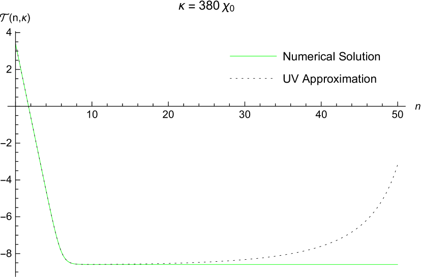
(a) $n_{\kappa}\simeq 6.0$

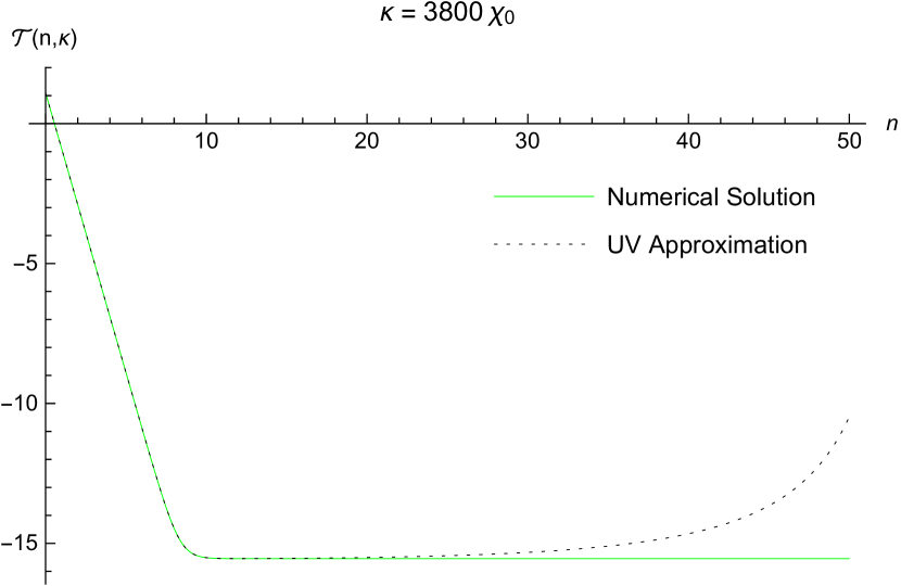
(b) $n_{\kappa}\simeq 8.3$

(c) $n_{\kappa}\simeq 10.0$

Figure 4.1: Plots the massless, minimally coupled scalar amplitude $\mathcal{T}(n,\kappa)$ (in solid green) and the (black dashed) ultraviolet approximation (4.109) versus the e-folding $n$ for three different values of $\kappa$.

Of course expression (4.109) is an approximation to the exact result. Because we propose to use this to compute the divergent coincidence limit of the propagator it is important to see how well $\mathcal{T}_{1}(n,\kappa)$ captures the ultraviolet behavior of $\mathcal{T}(n,\kappa)$. Because (4.109) is exact for constant first slow roll parameter, the deviation must involve derivatives of $\epsilon(n)$. It turns out to fall off like $\kappa^{-4}$ [Brooker:2015iya],

$$\mathcal{T}(n,\kappa)-\mathcal{T}_{1}(n,\kappa)=\Bigl{(}\frac{D\!-\!2}{16}\Bigr{)}\Bigl{[}(D+5-7\epsilon)\epsilon^{\prime}+\epsilon^{\prime\prime}\Bigr{]}\Bigl{(}\frac{\chi e^{n}}{\kappa}\Bigr{)}^{4}+O\Biggl{(}\Bigl{(}\frac{\chi e^{n}}{\kappa}\Bigr{)}^{6}\Biggr{)}.$$ (4.111)

We will see in section 4 that this suffices for an exact description of the ultraviolet.

The discrepancy between $\mathcal{T}(n,\kappa)$ and $\mathcal{T}_{1}(n,\kappa)$ that is evident at late times in Figure 4.1 is due to evolution of the first slow roll parameter $\epsilon(n)$. Figure 4.2 shows that the asymptotic late time phase is captured with great accuracy by the form,

$$\mathcal{T}_{2}(n,\kappa)=\ln\Biggl{[}\frac{\chi^{2}(n_{\kappa})}{2\kappa^{3}}\times C\Bigl{(}\epsilon(n_{\kappa})\Bigr{)}\Biggr{]}\;,$$ (4.112)

where the nearly unit correction factor $C(\epsilon)$ is,

$$C(\epsilon)\equiv\frac{1}{\pi}\Gamma^{2}\Bigl{(}\frac{1}{2}+\frac{1}{1\!-\!\epsilon}\Bigr{)}[2(1\!-\!\epsilon)]^{\frac{2}{1-\epsilon}}\;.$$ (4.113)

(a) $n_{\kappa}\simeq 6.0$

(b) $n_{\kappa}\simeq 8.3$

(c) $n_{\kappa}\simeq 10.0$

Figure 4.2: Plots the massless, minimally coupled scalar amplitude $\mathcal{T}(n,\kappa)$ (in solid green) and the (black dashed) late time approximation (4.112) versus the e-folding $n$ for three different values of $\kappa$.

Expression (4.112) is exact for constant $\epsilon(n)$. When the first slow roll parameter evolves there are very small nonlocal corrections whose form is known [Brooker:2017kjd] but whose net contribution is negligible for smooth potentials.

4.3.3 Temporal Photon

The temporal photon amplitude is very similar to the massive scalar which was the subject of a previous study [Kyriazis:2019xgj]. Like that system, the functional form of the amplitude is controlled by two key events:

1. First horizon crossing at $n_{\kappa}$ such that $\kappa e^{-n_{\kappa}}=\chi(n_{\kappa})$; and

2. Mass domination at $n_{\mu}$ such that $\mu=\frac{1}{2}\chi(n_{\mu})$.

The ultraviolet is well approximated by the form that applies for constant $\epsilon(n)$ and $\mu\propto\chi(n)$ [Janssen:2009pb],

$$\mathcal{U}_{1}(n,\kappa,\mu)\equiv\ln\Biggl{[}\frac{\frac{\pi}{2}z(n,\kappa)}{2\kappa e^{(D-2)n}}\Bigl{|}H^{(1)}_{\nu_{u}(n,\mu)}\Bigl{(}z(n,\kappa)\Bigr{)}\Bigr{|}^{2}\Biggr{]},$$ (4.114)

where the temporal index is,

$$\nu^{2}_{u}(n,\mu)\equiv\frac{1}{4}\Bigl{(}\frac{D\!-\!3\!+\!\epsilon(n)}{1\!-\!\epsilon(n)}\Bigr{)}^{2}\!\!-\frac{\mu^{2}}{[1\!-\!\epsilon(n)]^{2}\chi^{2}(n)}.$$ (4.115)

Figure 4.3 shows that the ultraviolet approximation is excellent when matter domination comes either before or after inflation.

(a) $n_{\mu}<0$

(b) $n_{\mu}<0$

(c) $n_{\mu}>50$

Figure 4.3: Plots the temporal amplitude $\mathcal{U}(n,\kappa,\mu)$ and the ultraviolet approximation (4.114) versus the e-folding $n$ for $\kappa=3800\chi_{0}$ (with $n_{\kappa}\simeq 8.3$) and three different values of $\mu$ with outside the range of inflation.

The ultraviolet regime is $\kappa e^{-n}\gg\{\chi(n),\mu\}$. To see how well the ultraviolet approximation captures this regime we substitute the difference into the exact evolution equation (4.105) and expand in powers of $e^{n}\chi(n)/\kappa$ to find [Kyriazis:2019xgj],

$$\mathcal{U}(n,\kappa,\mu)-\mathcal{U}_{1}(n,\kappa,\mu)=\Biggl{\{}\Bigl{(}5\epsilon-3\epsilon^{2}\Bigr{)}\frac{\mu^{2}}{4\chi^{2}}$$ (4.116)

$$\hskip 51.21504pt+\Bigl{(}\frac{D\!-\!2}{16}\Bigr{)}\Bigl{[}(D-9+7\epsilon)\epsilon^{\prime}-\epsilon^{\prime\prime}\Bigr{]}\Biggr{\}}\Bigl{(}\frac{\chi e^{n}}{\kappa}\Bigr{)}^{4}\!+O\Biggl{(}\Bigl{(}\frac{\chi e^{n}}{\kappa}\Bigr{)}^{6}\Biggr{)}.\qquad$$

This is suffices to give an exact result for the ultraviolet so we that can take the unregulated limit of $D=4$ for the approximations which pertain for $n>n_{\kappa}$.

The various terms in equation (4.105) behave differently before and after first horizon crossing. Evolution before first horizon crossing is controlled by the 4th and 7th terms,

$$\frac{2\kappa^{2}e^{-2n}}{\chi^{2}}-\frac{e^{-2(D-1)n-2\mathcal{U}}}{2\chi^{2}}\simeq 0\qquad\Longrightarrow\qquad\mathcal{U}\simeq-\ln(2\kappa)-(D\!-\!2)n\;.$$ (4.117)

After first horizon crossing these terms rapidly redshift into insignificance. We can take the unregulated limit ($D=4$), and equation (4.105) becomes,

$$\mathcal{U}^{\prime\prime}+\frac{1}{2}{\mathcal{U}^{\prime}}^{2}+(3\!-\!\epsilon)\mathcal{U}^{\prime}+4(1\!-\!\epsilon)+\frac{2\mu^{2}}{\chi^{2}}\simeq 0\;.$$ (4.118)

This is a nonlinear, first order equation for $\mathcal{U}^{\prime}$. Following [Kyriazis:2019xgj] we make the ansatz,

$$\mathcal{U}^{\prime}\simeq\alpha+\beta\tanh(\gamma)\;.$$ (4.119)

Substituting (4.119) in (4.118) gives,

$$\Bigl{(}{\rm Eqn.\ \ref{scUlate}}\Bigr{)}=\alpha^{\prime}+\frac{1}{2}\alpha^{2}+\frac{1}{2}\beta^{2}+(3\!-\!\epsilon)\alpha+4(1\!-\!\epsilon)+\frac{2\mu^{2}}{\chi^{2}}$$ (4.120)

$$\hskip 76.82234pt+\Bigl{[}(3\!-\!\epsilon\!+\!\alpha)\beta+\beta^{\prime}\Bigr{]}\tanh(\gamma)+\beta\Bigl{(}\gamma^{\prime}-\frac{1}{2}\beta\Bigr{)}{\rm sech}^{2}(\gamma)\;.\qquad$$

Ansatz (4.119) does not quite solve (4.118), but the following choices reduce the residue to terms of order $\epsilon\times\tanh(\gamma)$,

$$\alpha=-3\qquad,\qquad\frac{1}{4}\beta^{2}=\frac{1}{4}+\frac{\epsilon}{2}-\frac{\mu^{2}}{\chi^{2}}\qquad,\qquad\gamma^{\prime}=\frac{1}{2}\beta\;.$$ (4.121)

Figures 4.4 and 4.5 show how $\mathcal{U}(n,\kappa,\mu)$ behaves when mass domination comes after first horizon crossing and before the end of inflation.

Figure 4.4: Plots the temporal amplitude $\mathcal{U}(n,3800\chi_{0},0.4\chi_{0})$ and the three approximations: (4.114), (4.123) and (4.124). For $\kappa=3800\chi_{0}$ horizon crossing occurs at $n_{\kappa}\simeq 8.3$; for $\mu=0.4\chi_{0}$ mass domination occurs at $n_{\mu}\simeq 20.2$.

First comes a phase of slow decline followed by a period of oscillations. From (4.119) with (4.121) we see that these phases are controlled by a “frequency” defined as,

$$\omega^{2}_{u}(n,\mu)\equiv\frac{1}{4}+\frac{\epsilon(n)}{2}-\frac{\mu^{2}}{\chi^{2}(n)}\equiv-\Omega^{2}_{u}(n,\mu)\;.$$ (4.122)

During the phase of slow decline $\omega^{2}_{u}(n,\mu)>0$. Integrating (4.119) with (4.121) for this case gives,

$$\mathcal{U}_{2}(n,\kappa,\mu)=\mathcal{U}_{2}-3(n\!-\!n_{2})+2\ln\Biggl{[}\cosh\Bigl{(}\int_{n_{2}}^{n}\!\!\!dn^{\prime}\omega_{u}(n^{\prime},\mu)\Bigr{)}$$ (4.123)

$$\hskip 142.26378pt+\Bigl{(}\frac{3\!+\!\mathcal{U}_{2}^{\prime}}{2\omega_{u}(n_{2},\mu)}\Bigr{)}\sinh\Bigl{(}\int_{n_{2}}^{n}\!\!\!dn^{\prime}\omega_{u}(n^{\prime},\mu)\Bigr{)}\Biggr{]},\qquad$$

where $n_{2}\equiv n_{\kappa}+4$. The oscillatory phase is characterized by $\omega^{2}_{u}(n,\mu)<0$. Integrating (4.119) with (4.121) for this case produces,

$$\mathcal{U}_{3}(n,\kappa,\mu)=\mathcal{U}_{3}-3(n\!-\!n_{3})+2\ln\Biggl{[}\Biggl{|}\cos\Bigl{(}\int_{n_{3}}^{n}\!\!\!dn^{\prime}\Omega_{u}(n^{\prime},\mu)\Bigr{)}$$ (4.124)

$$\hskip 142.26378pt+\Bigl{(}\frac{3\!+\!\mathcal{U}_{3}^{\prime}}{2\Omega_{u}(n_{3},\mu)}\Bigr{)}\sin\Bigl{(}\int_{n_{3}}^{n}\!\!\!dn^{\prime}\Omega_{u}(n^{\prime},\mu)\Bigr{)}\Biggr{|}\Biggr{]},\qquad$$

where $n_{3}\equiv n_{\mu}+4$. Figures 4.4 and 4.5 show that these approximations are excellent.

Figure 4.5: Plots the temporal amplitude $\mathcal{U}(n,3800\chi_{0},0.3\chi_{0})$ and the three approximations: (4.114), (4.123) and (4.124). For $\kappa=3800\chi_{0}$ horizon crossing occurs at $n_{\kappa}\simeq 8.3$; for $\mu=0.3\chi_{0}$ mass domination occurs at $n_{\mu}\simeq 36.0$.

It is worth noting that the approximations (4.123) and (4.124) depend on $\kappa$ principally through the integration constants $\mathcal{U}_{2}\equiv\mathcal{U}(n_{2},\kappa,\mu)$ and $\mathcal{U}_{3}\equiv\mathcal{U}(n_{3},\kappa,\mu)$. Figure 4.6 shows the difference $\mathcal{U}(n,400\chi_{0},\mu)-\mathcal{U}(n,3800\chi_{0},\mu)$ for the same two choices of $\mu$ in Figures 4.4 and 4.5. One can see that the difference freezes into a constant after first horizon crossing to better than five significant figures!

Figure 4.6: Plots the difference of the temporal amplitude $\Delta\mathcal{U}\equiv\mathcal{U}(n,\kappa_{1},\mu)-\mathcal{U}(n,\kappa_{2},\mu)$ for $\kappa_{1}=400\chi_{0}$ and $\kappa_{2}=3800\chi_{0}$ with $\mu$ chosen so that all three approximations (4.114), (4.123) and (4.124) are necessary.

4.3.4 Spatially Transverse Photons

The general considerations for the amplitude of spatially transverse photons are similar to those for temporal photons. Before first horizon crossing it is the 4th and last terms of equation (4.107) which control the evolution,

$$\frac{2\kappa^{2}e^{-2n}}{\chi^{2}}-\frac{e^{-2(D-3)n-2\mathcal{V}}}{2\chi^{2}}\simeq 0\qquad\Longrightarrow\qquad\mathcal{V}\simeq-\ln(2\kappa)-(D\!-\!4)n\;.$$ (4.125)

A more accurate approximation is,

$$\mathcal{V}_{1}(n,\kappa,\mu)\equiv\ln\Biggl{[}\frac{\frac{\pi}{2}z(n,\kappa)}{2\kappa e^{(D-4)n}}\Bigl{|}H^{(1)}_{\nu_{v}(n,\mu)}\Bigl{(}z(n,\kappa)\Bigr{)}\Bigr{|}^{2}\Biggr{]},$$ (4.126)

where $z(n,\kappa)$ is the same as (4.110) and the transverse index is,

$$\nu^{2}_{v}(n,\mu)\equiv\frac{1}{4}\Bigl{(}\frac{D\!-\!3\!-\!\epsilon(n)}{1\!-\!\epsilon(n)}\Bigr{)}^{2}-\frac{\mu^{2}}{[1\!-\!\epsilon(n)]^{2}\chi^{2}(n)}\;.$$ (4.127)

Note the slight (order $\epsilon$) difference between $\nu^{2}_{u}(n,\mu)$ and $\nu^{2}_{v}(n,\mu)$. Figure 4.7 shows that (4.126) is excellent up to several e-foldings after first horizon crossing, and throughout inflation for $n_{\mu}<0$.

(a) $n_{\mu}<0$

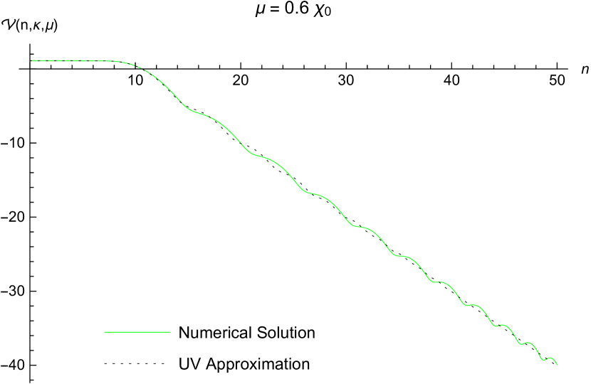
(b) $n_{\mu}<0$

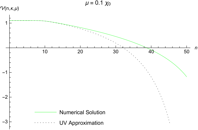
(c) $n_{\mu}>50$

Figure 4.7: Plots the transverse amplitude $\mathcal{V}(n,\kappa,\mu)$ and the ultraviolet approximation (4.126) versus the e-folding $n$ for $\kappa=3800\chi_{0}$ (with $n_{\kappa}\simeq 8.3$) and three different values of $\mu$ with outside the range of inflation.

Expression (4.126) also models the ultraviolet to high precision,

$$\mathcal{V}(n,\kappa,\mu)-\mathcal{V}_{1}(n,\kappa,\mu)=\Biggl{\{}\Bigl{(}5\epsilon-3\epsilon^{2}\Bigr{)}\frac{\mu^{2}}{4\chi^{2}}$$ (4.128)

$$\hskip 51.21504pt+\Bigl{(}\frac{D\!-\!4}{16}\Bigr{)}\Bigl{[}(D+3-7\epsilon)\epsilon^{\prime}+\epsilon^{\prime\prime}\Bigr{]}\Biggr{\}}\Bigl{(}\frac{\chi e^{n}}{\kappa}\Bigr{)}^{4}\!+O\Biggl{(}\Bigl{(}\frac{\chi e^{n}}{\kappa}\Bigr{)}^{6}\Biggr{)}.\qquad$$

Figure 4.8 shows $\mathcal{V}(n,\kappa,\mu)$ for the case where $n_{\mu}$ happens after first horizon crossing and before the end of inflation. One sees the same phases of slow decline after first horizon crossing, followed by oscillations.

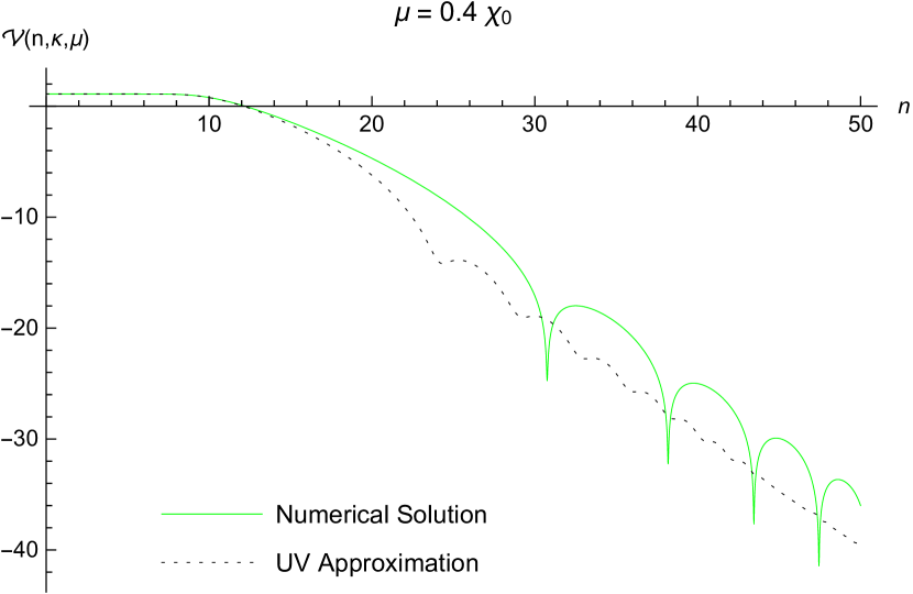
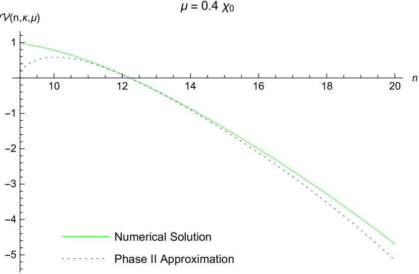
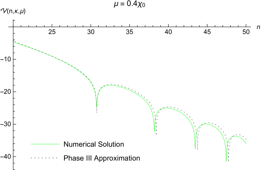
Figure 4.8: Plots the transverse amplitude $\mathcal{V}(n,3800\chi_{0},0.4\chi_{0})$ and the three approximations: (4.126), (4.131) and (4.132). For $\kappa=3800\chi_{0}$ horizon crossing occurs at $n_{\kappa}\simeq 8.3$; for $\mu=0.4\chi_{0}$ mass domination occurs at $n_{\mu}\simeq 20.2$.

The second and third phases can be understood by noting that the two terms of expression (4.125) redshift into insignificance after first horizon crossing. We can also set $D=4$ so that equation (4.107) degenerates to,

$$\mathcal{V}^{\prime\prime}+\frac{1}{2}{\mathcal{V}^{\prime}}^{2}+(1\!-\!\epsilon)\mathcal{V}^{\prime}+\frac{2\mu^{2}}{\chi^{2}}\simeq 0\;.$$ (4.129)

The same ansatz (4.119) applies to this regime, with the parameter choices,

$$\alpha=-1\quad,\quad\frac{1}{4}\beta^{2}=\frac{1}{4}-\frac{\mu^{2}}{\chi^{2}}\equiv\omega^{2}_{v}\equiv-\Omega^{2}_{v}\quad,\quad\gamma^{\prime}=\frac{1}{2}\beta\;.$$ (4.130)

Just as there was an order $\epsilon$ difference between the temporal and transverse indices — expressions (4.110) and (4.127), respectively — so too there is an order $\epsilon$ difference between $\omega^{2}_{u}(n,\mu)$ and $\omega^{2}_{v}(n,\kappa)$.

Integrating (4.119) with (4.130) for $\omega^{2}_{v}(,\mu)>0$ gives,

$$\mathcal{V}_{2}(n,\kappa,\mu)=\mathcal{V}_{2}-(n\!-\!n_{2})+2\ln\Biggl{[}\cosh\Bigl{(}\int_{n_{2}}^{n}\!\!\!dn^{\prime}\omega_{v}(n^{\prime},\mu)\Bigr{)}$$ (4.131)

$$\hskip 142.26378pt+\Bigl{(}\frac{1\!+\!\mathcal{V}_{2}^{\prime}}{2\omega_{v}(n_{2},\mu)}\Bigr{)}\sinh\Bigl{(}\int_{n_{2}}^{n}\!\!\!dn^{\prime}\omega_{v}(n^{\prime},\mu)\Bigr{)}\Biggr{]},\qquad$$

where $n_{2}\equiv n_{\kappa}+4$. Integrating (4.119) with (4.130) for $\omega^{2}_{v}(n,\mu)<0$ results in,

$$\mathcal{V}_{3}(n,\kappa,\mu)=\mathcal{V}_{3}-(n\!-\!n_{3})+2\ln\Biggl{[}\Biggl{|}\cos\Bigl{(}\int_{n_{3}}^{n}\!\!\!dn^{\prime}\Omega_{v}(n^{\prime},\mu)\Bigr{)}$$ (4.132)

$$\hskip 142.26378pt+\Bigl{(}\frac{1\!+\!\mathcal{V}_{3}^{\prime}}{2\Omega_{v}(n_{3},\mu)}\Bigr{)}\sin\Bigl{(}\int_{n_{3}}^{n}\!\!\!dn^{\prime}\Omega_{v}(n^{\prime},\mu)\Bigr{)}\Biggr{|}\Biggr{]},\qquad$$

where $n_{3}\equiv n_{\mu}+4$. Figures 4.8 and 4.9 demonstrate that the (4.131) and (4.132) approximations are excellent.

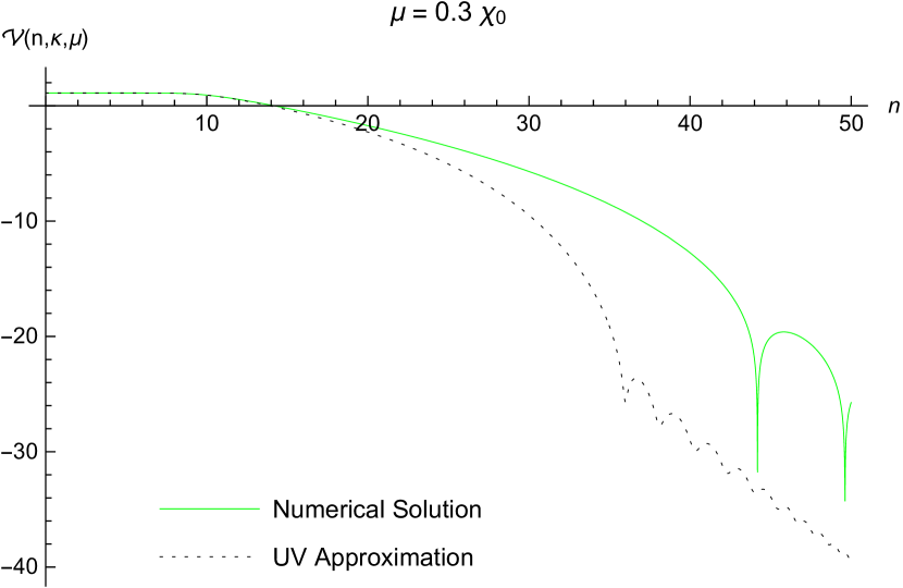
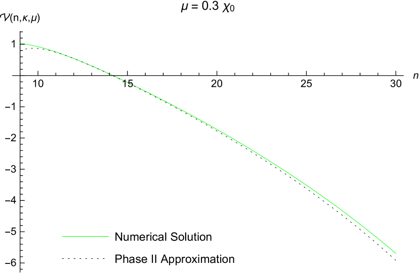
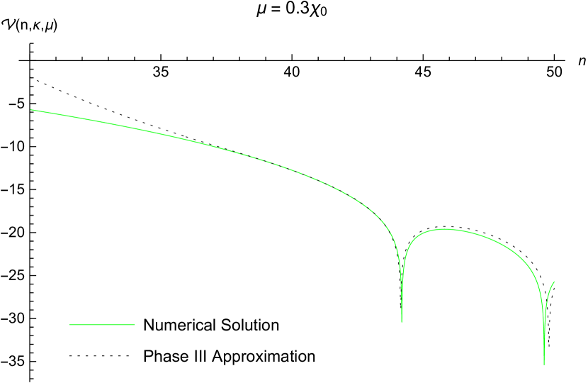
Figure 4.9: Plots the transverse amplitude $\mathcal{V}(n,3800\chi_{0},0.3\chi_{0})$ and the three approximations: (4.126), (4.131) and (4.132). For $\kappa=3800\chi_{0}$ horizon crossing occurs at $n_{\kappa}\simeq 8.3$; for $\mu=0.3\chi_{0}$ mass domination occurs at $n_{\mu}\simeq 36.0$.

Finally, we note that from Figure 4.10 that $\mathcal{V}^{\prime}(n,\kappa,\mu)$ is nearly independent of $\kappa$ after first horizon crossing.

Figure 4.10: Plots the difference of the transverse amplitude $\Delta\mathcal{V}\equiv\mathcal{V}(n,\kappa_{1},\mu)-\mathcal{V}(n,\kappa_{2},\mu)$ for $\kappa_{1}=400\chi_{0}$ and $\kappa_{2}=3800\chi_{0}$ with $\mu$ chosen so that all three approximations (4.126), (4.131) and (4.132) are necessary.

One consequence for the (4.131) and (4.132) approximations is that only the integration constants $\mathcal{V}_{2}$ and $\mathcal{V}_{3}$ depend on $\kappa$.

4.3.5 Plateau Potentials

We chose the quadratic dimensionless potential $U(\psi\psi^{*})=c^{2}\psi\psi^{*}$ for detailed studies because it gives simple, analytic expressions (4.100) in the slow roll approximation for the dimensionless Hubble parameter $\chi(n)$ and the first slow roll parameter $\epsilon(n)$. Setting $c\simeq 7.126\times 10^{-6}$ makes this model consistent with the observed values for the scalar amplitude and the scalar spectral index [Aghanim:2018eyx]. On the other hand, the model’s large prediction of $r\simeq 0.14$ is badly discordant with limits on the tensor-to-scalar ratio [Aghanim:2018eyx]. We shall therefore briefly consider how our analytic approximations fare when used with the plateau potentials currently consistent with observation.

The best known plateau potential is the Einstein-frame version of Starobinsky’s famous $R+R^{2}$ model [Starobinsky:1980te]. Expressing the dimensionless potential for this model in our notation gives [Brooker:2016oqa],

$$U(\psi\psi^{*})=\frac{3}{4}M^{2}\Bigl{(}1-e^{-\sqrt{\frac{2}{3}}\,|\psi|}\Bigr{)}^{2}\qquad,\qquad M=1.3\times 10^{-5}\;.$$ (4.133)

Somewhat over 50 e-foldings of inflation result if one starts from $\psi_{0}=4.6$, and the choice of $M=1.3\times 10^{-5}$ makes the model consistent with observation [Aghanim:2018eyx]. Figure 4.11 shows why $r=16\epsilon$ is so small for this model: its dimensionless Hubble parameter $\chi(n)$ is nearly constant.

Figure 4.11: Potential and geometry for the Einstein-frame representation of Starobinsky’s original model of inflation [Starobinsky:1980te]. The left shows the dimensionless potential $U(\psi\psi^{*})$ (4.133); the middle plot gives the dimensionless Hubble parameter $\chi(n)$ and the right hand plot depicts the first slow roll parameter $\epsilon(n)$. Inflation was assumed to start from $\psi_{0}=4.6$.

Figure 4.12: The left hand plot shows the amplitude $\mathcal{T}(n,\kappa)$ of the massless, minimally coupled scalar for $\kappa=3800\chi_{0}$, which corresponds to $n_{\kappa}\simeq 8.3$. The right hand graph shows the frequency $\omega_{u}^{2}(n,\mu)\simeq\omega^{2}_{v}(n,\mu)$ for $\mu=0.497\chi_{0}$ which passes through zero at $n_{\mu}\simeq 12$.

All our approximations pertain for this model, but the general effect of $\chi(n)$ being so nearly constant is to increase the range over which the ultraviolet approximations pertain. The left hand plot of Figure 4.12 shows this for the MMCS amplitude $\mathcal{T}(n,\kappa)$. Because $\epsilon(n)$ is so small, the temporal and transverse frequencies are nearly equal $\omega^{2}_{u}(n,\mu)\simeq\omega^{2}_{v}(n,\mu)$ and nearly constant. The right hand plot of Figure 4.12 shows this for a carefully chosen value of $\mu=0.497\chi_{0}$ which causes mass domination to occur during inflation. For this case we can just see the second and third phases occur in Figure 4.13.

Figure 4.13: Plots of the temporal amplitude $\mathcal{U}(n,\kappa,\mu)$ (left) and the spatially transverse amplitude $\mathcal{V}(n,\kappa,\mu)$ (right) versus $n$ for the Starobinsky potential (4.133). For each amplitude $\kappa=3800\chi_{0}$ (which implies $n_{\kappa}\simeq 8.3$) and $\mu=0.497\chi_{0}$ (which implies $n_{\mu}\simeq 12$).

4.4 Effective Potential

The purpose of this section is to evaluate the one photon loop contribution to the inflaton effective potential defined by equation (4.6). We begin by deriving some exact results for the trace of the coincident propagator, and we recall that $\mathcal{T}(n,\kappa)$ can be obtained from $\mathcal{U}(n,\kappa,0)$. Then the ultraviolet approximations (4.114) and (4.126) are used to derive a divergent result whose renormalization gives the part of the effective potential that depends locally on the geometry. We give large field and small field expansions for this local part, and we study its dependence on derivatives of $\epsilon(n)$. The section closes with a discussion of the nonlocal part of the effective potential which derives from the late time approximations (4.123), (4.124), (4.131) and (4.132).

4.4.1 Trace of the Coincident Photon Propagator

At coincidence the mixed time-space components of the photon mode sum vanish, and factors of $\widehat{k}_{m}\widehat{k}_{n}$ average to $\delta_{mn}/(D-1)$,

$$i\Bigl{[}\mbox{}_{\mu}\Delta_{\nu}\Bigr{]}(x;x)=\int\!\!\frac{d^{D-1}k}{(2\pi)^{D-1}}\,\Biggl{\{}\frac{1}{M^{2}}\left(\begin{matrix}k^{2}uu^{*}&0\cr 0&\frac{\delta_{mn}}{D-1}\mathcal{D}u\mathcal{D}u^{*}\end{matrix}\right)$$ (4.134)

$$\hskip 51.21504pt-\frac{1}{M^{2}}\left(\begin{matrix}\partial_{0}t\partial_{0}t^{*}&0\cr 0&\frac{\delta_{mn}}{D-1}k^{2}tt^{*}\end{matrix}\right)+\left(\begin{matrix}0&0\cr 0&(\frac{D-2}{D-1})\delta_{mn}vv^{*}\end{matrix}\right)\Biggr{\}}.\qquad$$

Its trace is,

$$g^{\mu\nu}i\Bigl{[}\mbox{}_{\mu}\Delta_{\nu}\Bigr{]}(x;x)=$$ (4.135)

$$\hskip 28.45274pt\int\!\!\frac{d^{D-1}k}{(2\pi)^{D-1}}\,\Biggl{\{}\frac{\mathcal{D}u\mathcal{D}u^{*}\!-\!k^{2}uu^{*}\!+\!\partial_{0}t\partial_{0}t^{*}\!-\!k^{2}tt^{*}}{a^{2}M^{2}}+\frac{(D\!-\!2)vv^{*}}{a^{2}}\Biggr{\}}.\qquad$$

Relation (4.55) allows us to replace the MMCS mode function $t(\eta,k)$ with the massless limit of the temporal mode function $u_{0}(\eta,k)\equiv u(\eta,k,0)$,

$$\partial_{0}t\partial_{0}t^{*}=k^{2}u_{0}u^{*}_{0}\qquad,\qquad k^{2}tt^{*}=\mathcal{D}u_{0}\mathcal{D}u^{*}_{0}\;.$$ (4.136)

Substituting (4.136) in (4.135) gives,

$$g^{\mu\nu}i\Bigl{[}\mbox{}_{\mu}\Delta_{\nu}\Bigr{]}(x;x)=$$ (4.137)

$$\hskip 22.76228pt\int\!\!\frac{d^{D-1}k}{(2\pi)^{D-1}}\,\Biggl{\{}\frac{\mathcal{D}u\mathcal{D}u^{*}\!-\!\mathcal{D}u_{0}\mathcal{D}u_{0}^{*}\!-\!k^{2}(uu^{*}\!-\!u_{0}u^{*}_{0})}{a^{2}M^{2}}+\frac{(D\!-\!2)vv^{*}}{a^{2}}\Biggr{\}}.\qquad$$

This second form (4.137) is very important because it demonstrates the absence of any $1/M^{2}$ pole as an exact relation, before any approximations are made.

The mode equation for temporal photons implies,

$$\mathcal{D}u\mathcal{D}u^{*}=a^{2}H^{2}\Bigl{[}u^{\prime}{u^{\prime}}^{*}+(D\!-\!2)(uu^{*})^{\prime}+(D\!-\!2)^{2}uu^{*}\Bigr{]}\;,$$ (4.139)

$$\hskip 22.76228pt=(k^{2}+a^{2}M^{2})uu^{*}+\frac{a^{2}H^{2}}{2}\Bigl{(}\partial_{n}\!+\!D\!-\!1\!-\!\epsilon\Bigr{)}\Bigl{(}\partial_{n}\!+\!2D\!-\!4\Bigr{)}(uu^{*})\;.\qquad$$

Using relations (4.139) and (4.137) allows us to express the trace of the coincident photon propagator in terms of three coincident scalar propagators,

$$g^{\mu\nu}i\Bigl{[}\mbox{}_{\mu}\Delta_{\nu}\Bigr{]}(x;x)=i\Delta_{u}(x;x)+\frac{(D\!-\!2)}{a^{2}}i\Delta_{v}(x;x)$$ (4.140)

$$\hskip 28.45274pt+\frac{H^{2}}{2M^{2}}\Bigl{(}\partial_{n}\!+\!D\!-\!1\!-\!\epsilon\Bigr{)}\Bigl{(}\partial_{n}\!+\!2D\!-\!4\Bigr{)}\Bigl{[}i\Delta_{u}(x;x)-i\Delta_{u_{0}}(x;x)\Bigr{]}\;.\qquad$$

The disappearance of any factors of $k^{2}$ from the Fourier mode sums in (4.140), coupled with the ultraviolet expansions (4.116) and (4.128), means that the phase 1 approximations $\mathcal{U}_{1}(n,\kappa,\mu)$ and $\mathcal{V}_{1}(n,\kappa,\mu)$ exactly reproduce the ultraviolet divergence structures.

Two of the scalar propagators in expression (4.140) are,

$$i\Delta_{u}(x;x^{\prime})\equiv\int\!\!\frac{d^{D-1}k}{(2\pi)^{D-1}}\Biggl{\{}\theta(\Delta\eta)u(\eta,k,M)u^{*}(\eta^{\prime},k,M)e^{i\vec{k}\cdot\Delta\vec{x}}$$ (4.141)

$$\hskip 128.0374pt+\theta(-\Delta\eta)u^{*}(\eta,k,M)u(\eta^{\prime},k,M)e^{-i\vec{k}\cdot\Delta\vec{x}}\Biggr{\}},\qquad$$

$$i\Delta_{v}(x;x^{\prime})\equiv\int\!\!\frac{d^{D-1}k}{(2\pi)^{D-1}}\Biggl{\{}\theta(\Delta\eta)v(\eta,k,M)v^{*}(\eta^{\prime},k,M)e^{i\vec{k}\cdot\Delta\vec{x}}$$ (4.142)

$$\hskip 128.0374pt+\theta(-\Delta\eta)v^{*}(\eta,k,M)v(\eta^{\prime},k,M)e^{-i\vec{k}\cdot\Delta\vec{x}}\Biggr{\}}.\qquad$$

The third scalar propagator $i\Delta_{u_{0}}(x;x^{\prime})$ is just the $M\rightarrow 0$ limit of $i\Delta_{u}(x;x^{\prime})$. The coincidence limits of each propagator can be expressed in terms of the corresponding amplitude,

$$\frac{i\Delta_{u}(x;x)}{\sqrt{8\pi G}}=\int\!\!\frac{d^{D-1}k}{(2\pi)^{D-1}}\,e^{\mathcal{U}(n,\kappa,\mu)}\quad,\quad\frac{i\Delta_{v}(x;x)}{\sqrt{8\pi G}}=\int\!\!\frac{d^{D-1}k}{(2\pi)^{D-1}}\,e^{\mathcal{V}(n,\kappa,\mu)}\;.$$ (4.143)

Expression(4.140) is exact but not immediately useful because we lack explicit expressions for the coincident propagators (4.143). It is at this stage that we must resort to the analytic approximations developed in section 3. Recall that the phase 1 approximation is valid until roughly 4 e-foldings after horizon crossing. If one instead thinks of this as a condition on the dimensionless wave number $\kappa\equiv\sqrt{8\pi G}\,k$ at fixed $n$, it means that $\kappa>\kappa_{n-4}$, where we define $\kappa_{n}$ as the dimensionless wave number which experiences horizon crossing at e-folding $n$. Taking as an example the temporal photon contribution we can write,

$$e^{\mathcal{U}(n,\kappa,\mu)}\simeq\theta\Bigl{(}\kappa\!-\!\kappa_{n-4}\Bigr{)}e^{\mathcal{U}_{1}(n,\kappa,\mu)}+\theta\Bigl{(}\kappa_{n-4}-\kappa\Bigr{)}e^{\mathcal{U}_{2,3}(n,\kappa,\mu)}\;,$$ (4.145)

$$\hskip 56.9055pt=e^{\mathcal{U}_{1}(n,\kappa,\mu)}+\theta\Bigl{(}\kappa_{n-4}-\kappa\Bigr{)}\Biggl{[}e^{\mathcal{U}_{2,3}(n,\kappa,\mu)}-e^{\mathcal{U}_{1}(n,\kappa,\mu)}\Biggr{]}.\qquad$$

Substituting the approximation (4.145) into expression (4.143) allows us to write,

$$i\Delta_{u}(x;x)\simeq L_{u}(n)+N_{u}(n)\;,$$ (4.146)

where we define the local ($L$) and nonlocal ($N$) contributions as,

$$L_{u}(n) \!\!\!\equiv\!\!\! \sqrt{8\pi G}\!\int\!\!\frac{d^{D-1}k}{(2\pi)^{D-1}}\,e^{\mathcal{U}_{1}(n,\kappa,\mu)}\;,$$ (4.147)

$$N_{u}(n) \!\!\!\equiv\!\!\! \sqrt{8\pi G}\!\int\!\!\frac{d^{3}k}{(2\pi)^{3}}\,\theta\Bigl{(}\kappa_{n-4}-\kappa\Bigr{)}\Biggl{[}e^{\mathcal{U}_{2,3}(n,\kappa,\mu)}-e^{\mathcal{U}_{1}(n,\kappa,\mu)}\Biggr{]}.\qquad$$ (4.148)

Note that we have taken the unregulated limit ($D=4$) in expression (4.148) because it is ultraviolet finite. The same considerations apply as well for the coincident spatially transverse photon propagator $i\Delta_{v}(x;x^{\prime})$, and for the massless limit of the temporal photon propagator $i\Delta_{u_{0}}(x;x)$.

4.4.2 The Local Contribution

The local contribution for each of the coincident propagators (4.143) comes from using the phase 1 approximation (4.147). For the temporal modes the amplitude is approximated by expression (4.114), whereupon we change variables to $z$ using $k=(1-\epsilon)Haz$, and then employ integral $6.574\;\#2$ of [Gradshteyn:1965],

$$L_{u}(n)=\frac{[(1\!-\!\epsilon)H]^{D-2}}{(4\pi)^{\frac{D}{2}}}\times\frac{\Gamma(\frac{D-1}{2}\!+\!\nu_{u})\Gamma(\frac{D-1}{2}\!-\!\nu_{u})}{\Gamma(\frac{1}{2}\!+\!\nu_{u})\Gamma(\frac{1}{2}\!-\!\nu_{u})}\times\Gamma\Bigl{(}1\!-\!\frac{D}{2}\Bigr{)}\;.$$ (4.149)

Recall that the index $\nu_{u}(n,\mu)$ is defined in expression (4.115). Of course the massless limit is,

$$L_{u_{0}}(n)=\frac{[(1\!-\!\epsilon)H]^{D-2}}{(4\pi)^{\frac{D}{2}}}\times\frac{\Gamma(\frac{D-1}{2}\!+\!\nu_{u_{0}})\Gamma(\frac{D-1}{2}\!-\!\nu_{u_{0}})}{\Gamma(\frac{1}{2}\!+\!\nu_{u_{0}})\Gamma(\frac{1}{2}\!-\!\nu_{u_{0}})}\times\Gamma\Bigl{(}1\!-\!\frac{D}{2}\Bigr{)}\;,$$ (4.150)

where the index is,

$$\nu_{u_{0}}(n)\equiv\nu_{u}(n,0)=\frac{1}{2}\Bigl{(}\frac{D\!-\!3\!+\!\epsilon(n)}{1\!-\!\epsilon(n)}\Bigr{)}\;.$$ (4.151)

The phase 1 approximation (4.126) for the transverse amplitude contains two extra scale factors which serve to exactly cancel the inverse scale factors that are evident in the transverse contribution to the trace of the coincident photon propagator (4.140). Hence we have,

$$\frac{L_{v}(n)}{a^{2}}=\frac{[(1\!-\!\epsilon)H]^{D-2}}{(4\pi)^{\frac{D}{2}}}\times\frac{\Gamma(\frac{D-1}{2}\!+\!\nu_{v})\Gamma(\frac{D-1}{2}\!-\!\nu_{v})}{\Gamma(\frac{1}{2}\!+\!\nu_{v})\Gamma(\frac{1}{2}\!-\!\nu_{v})}\times\Gamma\Bigl{(}1\!-\!\frac{D}{2}\Bigr{)}\;,$$ (4.152)

where the transverse index $\nu_{v}(n,\mu)$ is given in (4.127).

Each of the local contributions (4.149), (4.150) and (4.152) is proportional to the same divergent Gamma function,

$$\Gamma\Bigl{(}1\!-\!\frac{D}{2}\Bigr{)}=\frac{2}{D\!-\!4}+O\Bigl{(}(D\!-\!4)^{0}\Bigr{)}\;.$$ (4.153)

Each also contains a similar ratio of Gamma functions,

$$\frac{\Gamma(\frac{D-1}{2}\!+\!\nu)\Gamma(\frac{D-1}{2}\!-\!\nu)}{\Gamma(\frac{1}{2}\!+\!\nu)\Gamma(\frac{1}{2}\!-\!\nu)}=\Bigl{[}\Bigl{(}\frac{D\!-\!3}{2}\Bigr{)}^{2}\!-\!\nu^{2}\Bigr{]}\!\times\!\frac{\Gamma(\frac{D-3}{2}\!+\!\nu)\Gamma(\frac{D-3}{2}\!-\!\nu)}{\Gamma(\frac{1}{2}\!+\!\nu)\Gamma(\frac{1}{2}\!-\!\nu)}\;,$$ (4.155)

$$=\!\Bigl{[}\Bigl{(}\frac{D\!-\!3}{2}\Bigr{)}^{2}\!\!\!-\!\nu^{2}\Bigr{]}\Biggl{\{}\!1+\Bigl{[}\psi\Bigl{(}\frac{1}{2}\!+\!\nu\!\Bigr{)}\!+\!\psi\Bigl{(}\frac{1}{2}\!-\!\nu\!\Bigr{)}\Bigr{]}\Bigl{(}\frac{D\!-\!4}{2}\Bigr{)}\!+\!O\Bigl{(}(D\!-\!4)^{2}\Bigr{)}\!\Biggr{\}}.\qquad$$

These considerations allow us to break up each of the three terms in (4.140) into a potentially divergent part plus a manifestly finite part. For $i\Delta_{u}(x;x)\rightarrow L_{u}(n)$ this decomposition is,

$$L_{u}=\frac{[(1\!-\!\epsilon)H]^{D-4}}{(4\pi)^{\frac{D}{2}}}\Biggl{[}M^{2}-\frac{(D\!-\!2)H^{2}}{2}\Bigl{(}(D\!-\!3)\epsilon-\frac{1}{2}(D\!-\!4)\epsilon^{2}\Bigr{)}\Biggr{]}\Gamma\Bigl{(}1\!-\!\frac{D}{2}\Bigr{)}$$ (4.156)

$$\hskip 42.67912pt+\frac{1}{16\pi^{2}}\Bigl{[}M^{2}-\epsilon H^{2}\Bigr{]}\Bigl{[}\psi\Bigl{(}\frac{1}{2}\!+\!\nu_{u}\Bigr{)}+\psi\Bigl{(}\frac{1}{2}\!-\!\nu_{u}\Bigr{)}\Bigr{]}+O(D\!-\!4)\;.\qquad$$

For $(D-2)i\Delta_{v}(x;x)\rightarrow(D-2)L_{v}(n)$ we have,

$$(D\!-\!2)L_{v}=\frac{[(1\!-\!\epsilon)H]^{D-4}}{(4\pi)^{\frac{D}{2}}}\Biggl{[}(D\!-\!2)M^{2}-\frac{(D\!-\!2)(D\!-\!4)H^{2}}{2}\Bigl{(}(D\!-\!3)\epsilon$$ (4.157)

$$-\frac{(D\!-\!2)\epsilon^{2}}{2}\Bigr{)}\Biggr{]}\Gamma\Bigl{(}1\!-\!\frac{D}{2}\Bigr{)}+\frac{2M^{2}}{16\pi^{2}}\Bigl{[}\psi\Bigl{(}\frac{1}{2}\!+\!\nu_{v}\Bigr{)}+\psi\Bigl{(}\frac{1}{2}\!-\!\nu_{v}\Bigr{)}\Bigr{]}+O(D\!-\!4)\;.\qquad$$

And the final term in (4.140) — the one with derivatives — becomes,

$$\frac{H^{2}}{2M^{2}}\Bigl{(}\partial_{n}\!+\!D\!-\!1\!-\!\epsilon\Bigr{)}\Bigl{(}\partial_{n}\!+\!2D\!-\!4\Bigr{)}\Bigl{[}L_{u}\!-\!L_{u_{0}}\Bigr{]}=\frac{H^{2}}{2}\Bigl{(}\partial_{n}\!+\!D\!-\!1\!-\!\epsilon\Bigr{)}$$ (4.158)

$$\times\Bigl{(}\partial_{n}\!+\!2D\!-\!4\Bigr{)}\frac{[(1\!-\!\epsilon)H]^{D-4}}{(4\pi)^{\frac{D}{2}}}\Gamma\Bigl{(}1\!-\!\frac{D}{2}\Bigr{)}+\frac{H^{2}}{32\pi^{2}}\Bigl{(}\partial_{n}\!+\!3\!-\!\epsilon\Bigr{)}\Bigl{(}\partial_{n}\!+\!4\Bigr{)}\qquad$$

$$\hskip 28.45274pt\times\Biggl{\{}\psi\Bigl{(}\frac{1}{2}\!+\!\nu_{u}\Bigr{)}+\psi\Bigl{(}\frac{1}{2}\!-\!\nu_{u}\Bigr{)}-\frac{\epsilon H^{2}}{M^{2}}\Bigl{[}\psi\Bigl{(}\frac{1}{2}\!+\!\nu_{u}\Bigr{)}-\psi\Bigl{(}\frac{1}{2}\!+\!\nu_{u_{0}}\Bigr{)}$$

$$\hskip 128.0374pt+\psi\Bigl{(}\frac{1}{2}\!-\!\nu_{u}\Bigr{)}-\psi\Bigl{(}\frac{1}{2}\!-\!\nu_{u_{0}}\Bigr{)}\Bigr{]}\Biggr{\}}+O(D\!-\!4)\;.\qquad$$

Note that the difference $\psi(\frac{1}{2}\pm\nu_{u})-\psi(\frac{1}{2}\pm\nu_{u_{0}})$ is of order $M^{2}$ so expression (4.158) has no $1/M^{2}$ pole. Note also that the $1/\epsilon$ pole in $\psi(\frac{1}{2}-\nu_{u_{0}})=\psi(\frac{-\epsilon}{1-\epsilon})$ is canceled by an explicit multiplicative factor of $\epsilon$.

The potentially divergent terms (the ones proportional to $\Gamma(1-\frac{D}{2})$) in expressions (4.156), (4.157 and (4.158) sum to give,

$$(\ref{1stterm})_{\rm div}+(\ref{2ndterm})_{\rm div}+(\ref{3rdterm})_{\rm div}=\frac{[(1\!-\!\epsilon)H]^{D-4}}{(4\pi)^{\frac{D}{2}}}\Bigl{[}(D\!-\!1)M^{2}+\frac{1}{2}R\Bigr{]}\Gamma\Bigl{(}1\!-\!\frac{D}{2}\Bigr{)}$$ (4.159)

$$\hskip 19.91684pt+\frac{H^{2}}{16\pi^{2}}\Bigl{[}3-12\epsilon+4\epsilon^{2}-2\epsilon^{\prime}-\frac{(6\epsilon^{\prime}\!+\!\epsilon^{\prime\prime})}{1\!-\!\epsilon}-\Bigl{(}\frac{\epsilon^{\prime}}{1\!-\!\epsilon}\Bigr{)}^{2}\Bigr{]}+O(D\!-\!4)\;,\qquad$$

where we recall that the $D$-dimensional Ricci scalar is $R=(D-1)(D-2\epsilon)H^{2}$. Comparison with expression (4.6) for $\Delta V^{\prime}(\varphi\varphi^{*})$ reveals that we can absorb the divergences with the following counterterms,

$$\delta\xi=-\frac{\Gamma(1\!-\!\frac{D}{2})s^{D-4}}{(4\pi)^{\frac{D}{2}}}\times\frac{1}{2}q^{2}\qquad,\qquad\delta\lambda=-\frac{\Gamma(1\!-\!\frac{D}{2})s^{D-4}}{(4\pi)^{\frac{D}{2}}}\times 4(D\!-\!1)q^{4}\;,$$ (4.160)

where $s$ is the renormalization scale. Up to finite renormalizations, these choices agree with previous results [Miao:2015oba, Prokopec:2007ak, Miao:2019bnq], in the same gauge and using the same regularization, on de Sitter background.

Substituting expressions (4.156), (4.157), (4.158) and (4.160) into the definition (4.6) of $\Delta V^{\prime}(\varphi\varphi^{*})$ and taking the unregulated limit gives the local contribution,

$$\Delta V^{\prime}_{\rm L}(\varphi\varphi^{*})=\frac{q^{2}H^{2}}{16\pi^{2}}\Biggl{\{}\frac{(6M^{2}\!+\!R)}{2H^{2}}\ln\Bigl{[}\frac{(1\!-\!\epsilon)^{2}H^{2}}{s^{2}}\Bigr{]}\!+\!3\!-\!12\epsilon\!+\!4\epsilon^{2}\!-\!2\epsilon^{\prime}\!-\!\frac{(6\epsilon^{\prime}\!+\!\epsilon^{\prime\prime})}{1\!-\!\epsilon}$$ (4.161)

$$-\Bigl{(}\frac{\epsilon^{\prime}}{1\!-\!\epsilon}\Bigr{)}^{2}+\frac{M^{2}}{H^{2}}\Biggl{[}\psi\Bigl{(}\frac{1}{2}\!+\!\nu_{u}\Bigr{)}+\psi\Bigl{(}\frac{1}{2}\!-\!\nu_{u}\Bigr{)}+2\psi\Bigl{(}\frac{1}{2}\!+\!\nu_{v}\Bigr{)}+2\psi\Bigl{(}\frac{1}{2}\!-\!\nu_{v}\Bigr{)}\Biggr{]}$$

$$+\frac{1}{2}\Bigl{[}(\partial_{n}\!+\!3\!-\!\epsilon)(\partial_{n}\!+\!4)-2\epsilon\Bigr{]}\Bigl{[}\psi\Bigl{(}\frac{1}{2}\!+\!\nu_{u}\Bigr{)}\!+\!\psi\Bigl{(}\frac{1}{2}\!-\!\nu_{u}\Bigr{)}\Bigr{]}-(\partial_{n}\!+\!3\!-\!\epsilon)(\partial_{n}\!+\!4)$$

$$\hskip 51.21504pt\times\frac{\epsilon H^{2}}{2M^{2}}\Bigl{[}\psi\Bigl{(}\frac{1}{2}\!+\!\nu_{u}\Bigr{)}\!-\!\psi\Bigl{(}\frac{1}{1\!-\!\epsilon}\Bigr{)}+\psi\Bigl{(}\frac{1}{2}\!-\!\nu_{u}\Bigr{)}\!-\!\psi\Bigl{(}\frac{-\epsilon}{1\!-\!\epsilon}\Bigr{)}\Bigr{]}\Biggr{\}}.\qquad$$

It is worth noting that there are no singularities at $\epsilon=1$, or when either $1/(1-\epsilon)$ or $-\epsilon/(1-\epsilon)$ become non-positive integers [Janssen:2008px]. The effective potential is obtained by integrating (4.161) with respect to $\varphi\varphi^{*}$. The result is best expressed using the variable $z\equiv q^{2}\varphi\varphi^{*}/H^{2}$,

$$\Delta V_{\rm L}=\frac{H^{4}}{16\pi^{2}}\Biggl{\{}\!\Bigl{[}3z^{2}\!+\!\frac{Rz}{2H^{2}}\Bigr{]}\!\ln\Bigl{[}\frac{(1\!-\!\epsilon)^{2}H^{2}}{s^{2}}\Bigr{]}\!+\!\Bigl{[}3\!-\!12\epsilon\!+\!4\epsilon^{2}\!-\!2\epsilon^{\prime}\!-\!\frac{(6\epsilon^{\prime}\!+\!\epsilon^{\prime\prime})}{1\!-\!\epsilon}\Bigr{]}z$$ (4.162)

$$-\frac{{\epsilon^{\prime}}^{2}z}{(1\!-\!\epsilon)^{2}}+2\!\int_{0}^{z}\!\!\!dx\,x\Biggl{[}\psi\Bigl{(}\frac{1}{2}\!+\!\alpha\!\Bigr{)}\!+\!\psi\Bigl{(}\frac{1}{2}\!-\!\alpha\!\Bigr{)}\!+\!2\psi\Bigl{(}\frac{1}{2}\!+\!\beta\!\Bigr{)}\!+\!2\psi\Bigl{(}\frac{1}{2}\!-\!\beta\!\Bigr{)}\Biggr{]}$$

$$+\frac{1}{2}\Bigl{[}(\partial_{n}\!+\!3\!-\!3\epsilon)(\partial_{n}\!+\!4\!-\!2\epsilon)-2\epsilon\Bigr{]}\!\int_{0}^{z}\!\!\!dx\Bigl{[}\psi\Bigl{(}\frac{1}{2}\!+\!\alpha(x)\Bigr{)}+\psi\Bigl{(}\frac{1}{2}\!-\!\alpha(x)\Bigr{)}\Bigr{]}$$

$$-(\partial_{n}\!+\!3\!-\!3\epsilon)(\partial_{n}\!+\!4\!-\!2\epsilon)\!\int_{0}^{z}\!\!\frac{dx\epsilon}{4x}\Bigl{[}\psi\Bigl{(}\frac{1}{2}\!+\!\alpha(x)\Bigr{)}-\psi\Bigl{(}\frac{1}{1\!-\!\epsilon}\Bigr{)}$$

$$\hskip 184.9429pt+\psi\Bigl{(}\frac{1}{2}\!-\!\alpha(x)\Bigr{)}-\psi\Bigl{(}\frac{-\epsilon}{1\!-\!\epsilon}\Bigr{)}\Bigr{]}\Biggr{\}},\qquad$$

where the $x$-dependent indices are,

$$\alpha(x)\equiv\sqrt{\frac{1}{4}+\frac{\epsilon\!-\!2x}{(1\!-\!\epsilon)^{2}}}\qquad,\qquad\beta(x)\equiv\sqrt{\frac{1}{4}-\frac{2x}{(1\!-\!\epsilon)^{2}}}\;.$$ (4.163)

Note that the term inside the square brackets on the last line of (4.162) vanishes for $x=0$, so the integrand is well defined at $x=0$.

4.4.3 Large Field & Small Field Expansions

Expression (4.162) depends principally on the quantity $z=q^{2}\varphi\varphi^{*}/H^{2}$. During inflation $z$ is typically quite large, whereas it touches $0$ after the end of inflation. Figure 4.14 shows this for the quadratic potential, and the results are similar for the Starobinsky potential (4.133). It is therefore desirable to expand the potential $\Delta V_{L}(\varphi\varphi^{*})$ for large $z$ and for small $z$.

Figure 4.14: Plots of the dimensionless inflaton field $\psi(n)$ and the ratio $z\equiv q^{2}\psi^{2}/\chi^{2}$ after the end of inflation for the quadratic potential. Here we chose $q^{2}=\frac{1}{137}$.

The large field regime follows from the large argument expansion of the digamma function,

$$\psi(x)=\ln(x)-\frac{1}{2x}-\frac{1}{12x^{2}}+\frac{1}{120x^{4}}-\frac{1}{256x^{6}}+O\Bigl{(}\frac{1}{x^{8}}\Bigr{)}\;.$$ (4.164)

Substituting (4.164) in (4.162), and performing the various integrals gives,

$$\Delta V_{L}=\frac{H^{4}}{16\pi^{2}}\Biggl{\{}3z^{2}\ln\Bigl{(}\frac{2q^{2}\varphi\varphi^{*}}{s^{2}}\Bigr{)}\!-\!\frac{3}{2}z^{2}+\frac{Rz}{2H^{2}}\ln\Bigl{(}\frac{2q^{2}\varphi\varphi^{*}}{s^{2}}\Bigr{)}\!-\!(4\!+\!8\epsilon\!-\!3\epsilon^{2})z$$ (4.165)

$$\hskip 14.22636pt-\epsilon^{\prime}z-\Bigl{[}\frac{3}{4}\epsilon(1\!-\!\epsilon)(2\!-\!\epsilon)+\frac{7}{8}(1\!-\!\epsilon)\epsilon^{\prime}+\frac{1}{8}\epsilon^{\prime\prime}\Bigr{]}\ln^{2}(2z)+O\Bigl{(}\ln(z)\Bigr{)}\Biggr{\}}.\qquad$$

The leading contribution of (4.165) agrees with the famous flat space result of Coleman and Weinberg [Coleman:1973jx],

$$\Delta V\longrightarrow\frac{3(q^{2}\varphi\varphi^{*})^{2}}{16\pi^{2}}\ln\Bigl{(}\frac{2q^{2}\varphi\varphi^{*}}{s^{2}}\Bigr{)}\;.$$ (4.166)

The first three terms of (4.165) could be subtracted using allowed counterterms of the form $F(\varphi\varphi^{*},R)$ [Woodard:2006nt]. A prominent feature of the remaining terms is the presence of derivatives of the first slow roll parameter. These derivatives are typically very small during inflation but Figure 4.15 shows that they can be quite large after the end of inflation.

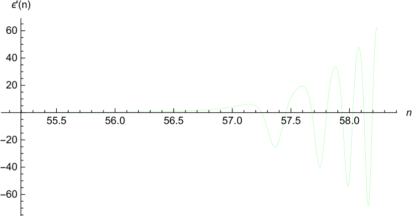
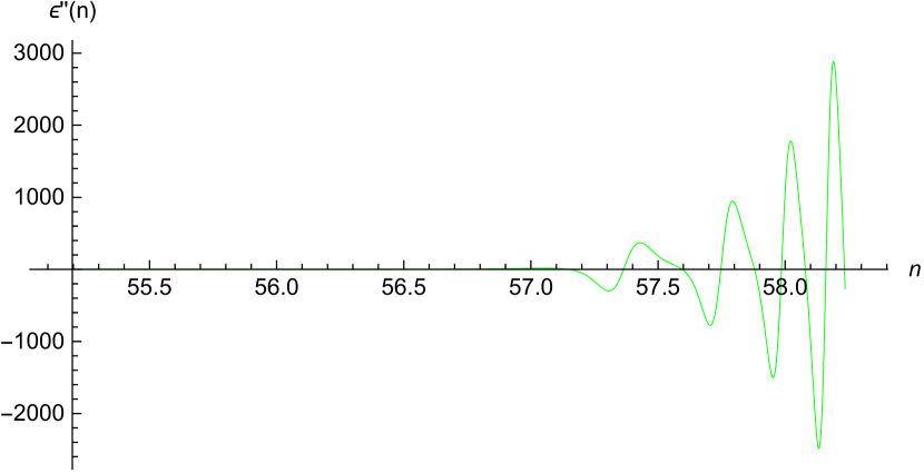
Figure 4.15: Plots of the first slow roll and its derivatives after the end of inflation for the quadratic potential.

The small field expansion derives from expanding the digamma functions in expression (4.162) in powers of $x$,

$$\psi\Bigl{(}\frac{1}{2}\!+\!\alpha(x)\Bigr{)} = \psi\Bigl{(}\frac{1}{1\!-\!\epsilon}\Bigr{)}-\psi^{\prime}\Bigl{(}\frac{1}{1\!-\!\epsilon}\Bigr{)}\frac{2x}{1\!-\!\epsilon^{2}}+O(x^{2})\;,$$ (4.167)

$$\psi\Bigl{(}\frac{1}{2}\!-\!\alpha(x)\Bigr{)} = \psi\Bigl{(}\frac{-\epsilon}{1\!-\!\epsilon}\Bigr{)}+\psi^{\prime}\Bigl{(}\frac{-\epsilon}{1\!-\!\epsilon}\Bigr{)}\frac{2x}{1\!-\!\epsilon^{2}}+O(x^{2})\;,$$ (4.168)

$$\psi\Bigl{(}\frac{1}{2}\!+\!\beta(x)\Bigr{)} = -\gamma-\frac{\pi^{2}}{6}\frac{2x}{(1\!-\!\epsilon)^{2}}+O(x^{2})\;,$$ (4.169)

$$\psi\Bigl{(}\frac{1}{2}\!-\!\beta(x)\Bigr{)} = -\frac{(1\!-\!\epsilon)^{2}}{2x}+1-\gamma+\Bigl{[}1\!+\!\frac{\pi^{2}}{6}\Bigr{]}\frac{2x}{(1\!-\!\epsilon)^{2}}+O(x^{2})\;.\qquad$$ (4.170)

The result is,

$$\Delta V_{L}=\frac{H^{4}}{16\pi^{2}}\Biggl{\{}\Biggl{[}\frac{R}{2H^{2}}\ln\Bigl{[}\frac{(1\!-\!\epsilon)^{2}H^{2}}{s^{2}}\Bigr{]}\!+\!1\!-\!8\epsilon\!+\!2\epsilon^{2}\!-\!2\epsilon^{\prime}-\frac{(6\epsilon^{\prime}\!+\!\epsilon^{\prime\prime})}{1\!-\!\epsilon}\!-\!\frac{{\epsilon^{\prime}}^{2}}{(1\!-\!\epsilon)^{2}}\Biggr{]}z$$ (4.171)

$$\hskip 56.9055pt+\frac{1}{2}\Bigl{[}(\partial_{n}\!+\!3\!-\!3\epsilon)(\partial_{n}\!+\!4\!-\!2\epsilon)\!-\!2\epsilon\Bigr{]}\Bigl{[}\psi\Bigl{(}\frac{1}{1\!-\!\epsilon}\Bigr{)}\!+\!\psi\Bigl{(}\frac{-\epsilon}{1\!-\!\epsilon}\Bigr{)}\Bigr{]}z$$

$$+\frac{1}{2}(\partial_{n}\!+\!3\!-\!3\epsilon)(\partial_{n}\!+\!4\!-\!2\epsilon)\Bigl{[}\psi^{\prime}\Bigl{(}\frac{1}{1\!-\!\epsilon}\Bigr{)}\!-\!\psi^{\prime}\Bigl{(}\frac{-\epsilon}{1\!-\!\epsilon}\Bigr{)}\Bigr{]}\frac{\epsilon z}{1\!-\!\epsilon^{2}}+O(z^{2})\Biggr{\}}.\qquad$$

Note that the $1/\epsilon$ pole from $\psi(\frac{-\epsilon}{1-\epsilon})$ on the penultimate line of (4.171) cancels against the double pole from $\psi^{\prime}(\frac{-\epsilon}{1-\epsilon})$ on the last line.

4.4.4 The Nonlocal Contribution

The nonlocal contribution to the effective potential is obtained by substituting the nonlocal contribution (4.148) to each coincident propagator in (4.140), and then into expression (4.6),

$$\Delta V^{\prime}_{\rm N}(\varphi\varphi^{*})=q^{2}N_{u}(n)+2q^{2}e^{-2n}N_{v}(n)$$ (4.172)

$$\hskip 113.81102pt+\frac{q^{2}H^{2}}{2M^{2}}\Bigl{(}\partial_{n}\!+\!3\!-\!\epsilon\Bigr{)}\Bigl{(}\partial_{n}\!+\!4\Bigr{)}\Bigl{[}N_{u}(n)\!-\!N_{u_{0}}(n)\Bigr{]}.\qquad$$

The nonlocal contributions to the various propagators are,

$$N_{u}(n) \!\!\!=\!\!\! \int_{0}^{\kappa_{n-4}}\!\!\frac{d\kappa\,\kappa^{2}}{32\pi^{3}G}\Biggl{[}e^{\mathcal{U}_{2,3}(n,\kappa,\mu)}-e^{\mathcal{U}_{1}(n,\kappa,\mu)}\Biggr{]},\qquad$$ (4.173)

$$N_{u_{0}}(n) \!\!\!=\!\!\! \int_{0}^{\kappa_{n-4}}\!\!\frac{d\kappa\,\kappa^{2}}{32\pi^{3}G}\Biggl{[}e^{\mathcal{U}_{2}(n,\kappa,0)}-e^{\mathcal{U}_{1}(n,\kappa,0)}\Biggr{]},\qquad$$ (4.174)

$$N_{v}(n) \!\!\!=\!\!\! \int_{0}^{\kappa_{n-4}}\!\!\frac{d\kappa\,\kappa^{2}}{32\pi^{3}G}\Biggl{[}e^{\mathcal{V}_{2,3}(n,\kappa,\mu)}-e^{\mathcal{V}_{1}(n,\kappa,\mu)}\Biggr{]}.\qquad$$ (4.175)

The nonlocal nature of these contributions derives from the integration over $\kappa$, which can be converted to an integration over $n_{\kappa}$,

$$\kappa\equiv e^{n_{\kappa}}\chi(n_{\kappa})\qquad\Longrightarrow\qquad\frac{d\kappa}{\kappa}=\Bigl{[}1\!-\!\epsilon(n_{\kappa})\Bigr{]}dn_{\kappa}\;.$$ (4.176)

After this is done, any factors of $\kappa$ depend on the earlier geometry.

A number of approximations result in huge simplification. First, note from Figures 4.4 and 4.5 that the ultraviolet approximation (4.114) for $\mathcal{U}(n,\kappa,\mu)$ is typically more negative than the late time approximations (4.123) and (4.124). Figures 4.8 and 4.9 show that the same rule applies to $\mathcal{V}(n,\kappa,\mu)$. Hence we can write,

$$N_{u}(n)\simeq\int_{0}^{\kappa_{n-4}}\!\!\frac{d\kappa\,\kappa^{2}}{16\pi^{3}G}\,e^{\mathcal{U}_{2,3}(n,\kappa,\mu)}\qquad,\qquad N_{v}(n)\simeq\int_{0}^{\kappa_{n-4}}\!\!\frac{d\kappa\,\kappa^{2}}{16\pi^{3}G}\,e^{\mathcal{V}_{2,3}(n,\kappa,\mu)}\;.$$ (4.177)

Second, because the temporal and transverse frequencies are nearly equal, we can write,

$$\omega^{2}_{u}(n,\mu)\simeq\omega^{2}_{v}(n,\mu)\qquad\Longrightarrow\qquad\mathcal{U}(n,\kappa,\mu)\simeq\mathcal{V}(n,\kappa,\mu)-2n\;.$$ (4.178)

When the mass vanishes there is so little difference between the ultraviolet approximation (4.114) and its late time extension (4.123) that we can ignore this contribution, $N_{u_{0}}(n)\simeq 0$. Next, Figures 4.6 and 4.10 imply that the late time approximations for $\mathcal{U}(n,\kappa,\mu)$ and $\mathcal{V}(n,\kappa,\mu)$ inherit their $\kappa$ dependence from the ultraviolet approximation at $n\simeq n_{\kappa}+4$, which is itself independent of $\mu$,

$$n>n_{\kappa}+4\qquad\Longrightarrow\qquad\mathcal{U}_{2,3}(n,\kappa,\mu)\simeq\mathcal{U}_{1}(n_{\kappa}\!+\!4,\kappa,0)+f_{2,3}(n,\mu)\;,$$ (4.179)

where $f_{2,3}(n,\mu)$ can be read off from expressions (4.123) and (4.124) by omitting the $\kappa$-dependent integration constants. Finally, we can use the slow roll form (4.112) for the amplitude reached after first horizon crossing and before the mass dominates,

$$e^{\mathcal{U}_{1}(n_{\kappa}+4,\kappa,0)}\simeq\frac{\chi^{2}(n_{\kappa})}{2\kappa^{3}}\times C\Bigl{(}\epsilon(n_{\kappa})\Bigr{)}\;.$$ (4.180)

Putting it all together gives,

$$\Delta V_{N}(\varphi\varphi^{*})\simeq 3q^{2}\!\!\int_{0}^{n-4}\!\!\!\!\!\!\!dn_{\kappa}\frac{[1\!-\!\epsilon(n_{\kappa})]\chi^{2}(n_{\kappa})C(n_{\kappa}))}{32\pi^{3}G}\times e^{f_{2,3}(n,\mu)}$$ (4.181)

$$+\frac{q^{2}\chi^{2}(n)}{2\mu^{2}}(\partial_{n}\!+\!3\!-\!\epsilon)(\partial_{n}\!+\!4)\!\!\int_{0}^{n-4}\!\!\!\!\!\!dn_{\kappa}\frac{[1\!-\!\epsilon(n_{\kappa})]\chi^{2}(n_{\kappa})C(\epsilon(n_{\kappa}))}{32\pi^{3}G}\!\times\!e^{f_{2,3}(n,\mu)}\!.\qquad$$

4.5 Conclusions

In section 2 we derived an exact, dimensionally regulated, Fourier mode sum (4.50) for the Lorentz gauge propagator of a massive photon on an arbitrary cosmological background (4.3). Our result is expressed in terms of mode functions $t(\eta,k)$, $u(\eta,k,M)$ and $v(\eta,k,M)$ whose defining relations are (4.10), (4.24) and (4.22), which respectively represent massless minimally coupled scalars, massive temporal photons, and massive spatially transverse photons. The photon propagator can also be expressed as a sum (4.51) of bi-vector differential operators acting on the scalar propagators $i\Delta_{t}(x;x^{\prime})$, $i\Delta_{u}(x;x^{\prime})$ and $i\Delta_{v}(x;x^{\prime})$ associated with the three mode functions. Because Lorentz gauge is an exact gauge there should be no linearization instability, even on de Sitter, such as occurs for Feynman gauge [Kahya:2005kj, Kahya:2006ui].

In section 3 we converted to a dimensionless form with time represented by the number of e-foldings $n$ since the beginning of inflation, and the wave number, mass and Hubble parameter all expressed in reduced Planck units, $\kappa\equiv\sqrt{8\pi G}\,k$, $\mu\equiv\sqrt{8\pi G}\,M$ and $\chi(n)\equiv\sqrt{8\pi G}\,H(\eta)$. Analytic approximations were derived for the amplitudes $\mathcal{T}(n,\kappa)$, $\mathcal{U}(n,\kappa,\mu)$ and $\mathcal{V}(n,\kappa,\mu)$ associated with each of the mode functions. Which approximation to use is controlled by first horizon crossing at $\kappa=e^{n_{\kappa}}\chi(n_{\kappa})$ and mass domination at $\mu=\frac{1}{2}\chi(n_{\mu})$. Until shortly after first horizon crossing we employ the ultraviolet approximations (4.109), (4.114) and (4.126). After first horizon crossing and before mass domination the appropriate approximations are (4.112), (4.123) and (4.131). And after mass domination (which $\mathcal{T}(n,\kappa)$ never experiences) the amplitudes are well approximated by (4.124) and (4.132). The validity of these approximations was checked against explicit numerical solutions for inflation driven by the simple quadratic model, and by the phenomenologically favored plateau model (4.133).

In section 4 we applied our approximations to compute the effective potential induced by photons coupled to a charged inflaton. Our result consists of a part (4.162) which depends locally on the geometry (4.3) and a numerically smaller part (4.181) which depends on the past history. The local part was expanded both for the case of large field strength (4.165), and for small field strength (4.171). The existence of the second, nonlocal contribution, was conjectured on the basis of indirect arguments [Miao:2015oba] that have now been explicitly confirmed. Another conjecture that has been confirmed is the rough validity of extrapolating de Sitter results [Allen:1983dg, Prokopec:2007ak] from the constant Hubble parameter of de Sitter background to the time dependent one of a general cosmological background (4.3). However, we now have good approximations for the dependence on the first slow roll parameter $\epsilon(n)$.

Our most important result is probably the fact that electromagnetic corrections to the effective potential depend upon first and second derivatives of the first slow roll parameter. One consequence is that the effective potential from electromagnetism responds more strongly to changes in the geometry than for scalars [Kyriazis:2019xgj] or spin one half fermions [Sivasankaran:2020dzp]. This can be very important during reheating (see Figure 4.15); it might also be significant if features occur during inflation. Another consequence is that there cannot be perfect cancellation between the positive effective potentials induced by bosons and the negative potentials induced by fermions [Miao:2020zeh]. Note that the derivatives of $\epsilon$ come exclusively from the constrained part of the photon propagator — the $t(\eta,k)$ and $u(\eta,k)$ modes — which is responsible for long range electromagnetic interactions. Dynamical photons — the $v(\eta,k)$ modes — produce no derivatives at all. These statements can be seen from expression (4.140), which is exact, independent of any approximation.

We close with a speculation based on the correlation between the spin of the field and the number of derivatives it induces in the effective potential: scalars produce no derivatives [Kyriazis:2019xgj], spin one half fermions induce one derivative [Sivasankaran:2020dzp], and this paper has shown that spin one vectors give two derivatives. It would be interesting to see if the progression continues for gravitinos (which ought to induce three derivatives) and gravitons (which would induce four derivatives). Of course gravitons do not acquire a mass through coupling to a scalar inflaton, but they do respond to it, and the mode equations have been derived in a simple gauge [Iliopoulos:1998wq, Abramo:2001dc]. Until now it was not possible to do much with this system because it can only be solved exactly for the case of constant $\epsilon(n)$, however, we now have a reliable approximation scheme that can be used for arbitrary $\epsilon(n)$. Further, we have a worthy object of study in the graviton 1-point function, which defines how quantum 0-point fluctuations back-react to change the classical geometry. At one loop order it consists of the same sort of coincident propagator we have studied in this paper. On de Sitter background the result is just a constant times the de Sitter metric [Tsamis:2005je], which must be absorbed into a renormalization of the cosmological constant if “$H$” is to represent the true Hubble parameter. Now suppose that the graviton propagator for general first slow roll parameter consists of a local part with up to 4th derivatives of $\epsilon(n)$ plus a nonlocal part. That sort of result could not be absorbed into any counterterm. So perhaps there is one loop back-reaction after all [Geshnizjani:2002wp], and de Sitter represents a case of unstable equilibrium?

Chapter 5 Reheating with Effective Potential

5.1 Introduction

Scalar-driven inflation is supported by the slow roll of the inflaton down its potential. At the end of inflation the inflaton begins oscillating, and its kinetic energy is transferred to ordinary matter during the process of reheating. The efficiency of this transfer obviously depends on the way the inflaton is coupled to ordinary matter. Ema et al. have shown that the most efficient coupling is that of a charged inflaton to electromagnetism [Ema:2016dny].

What happens is that the evolution of a charged inflaton induces a time-dependent photon mass which oscillates around zero during reheating. The temporal and longitudinal components of the photon diverge as the mass goes to zero, which makes reheating very efficient. The process has been previously studied by discretizing space, carrying out a finite Fourier transform, and then numerically evolving the nonlinear system of the inflaton plus electromagnetism [Bezrukov:2020txg]. However, the energy transfer is broadly distributed over so many modes that there is little point to including nonlinear effects in the photon field, provided that its response to the inflaton $0$-mode is known to all orders. In that case, one merely sums the contribution from each photon mode’s wave vector, which can be accomplished by varying the inflaton effective potential. The goal of this chapter is to develop a good analytic approximation for the massive photon propagator in a time-dependent inflaton background, and then use it to compute the quantum-induced, effective force in equation for the inflaton $0$-mode. In this way reheating can be studied by numerically solving a nonlocal equation for the inflaton $0$-mode.

This chapter consists of five sections, of which the first is this Introduction. In section 2 we derive a spatial Fourier mode sum for the massive photon propagator which is valid when the mass becomes time-dependent. Section 3 develops analytic approximations for the temporal and longitudinal modes, checking them against explicit numerical analysis for a simple model of inflation. In section 4 we discuss how these approximations can be used to estimate the quantum-induced effective force which controls the process of reheating. Section 5 gives our conclusions.

5.2 The Massive Photon Propagator

The purpose of this section is to generalize the massive photon propagator from its known form for a constant mass [Katuwal:2021kry] to the case of a time-dependent mass. The Lagrangian is,

$$\mathcal{L}=-\frac{1}{4}F_{\mu\nu}F_{\rho\sigma}g^{\mu\rho}g^{\nu\sigma}\sqrt{-g}$$ (5.1)

$$\hskip 56.9055pt-\Bigl{(}\partial_{\mu}\!-\!iqA_{\mu}\Bigr{)}\varphi\Bigl{(}\partial_{\nu}\!+\!iqA_{\nu}\Bigr{)}\varphi^{*}g^{\mu\nu}\sqrt{-g}-V(\varphi\varphi^{*})\sqrt{-g}\;,\qquad$$

where $\varphi$ is the inflaton and $F_{\mu\nu}\equiv\partial_{\mu}A_{\nu}-\partial_{\nu}A_{\mu}$ is the electromagnetic field strength. We work on a general homogeneous, isotropic and spatially flat geometry in $D$-dimensional, conformal coordinates, with Hubble parameter $H$ and first slow roll parameter $\epsilon$,

$$ds^{2}=a^{2}\Bigl{[}-d\eta^{2}+d\vec{x}\!\cdot\!d\vec{x}\Bigr{]}\qquad,\qquad H\equiv\frac{\partial_{0}a}{a^{2}}\quad,\quad\epsilon\equiv-\frac{\partial_{0}H}{aH^{2}}\;.$$ (5.2)

The section first reviews the constant mass case, and then makes the generalizations necessary to incorporate a time-dependent mass.

5.2.1 Constant Mass

When the photon’s mass is constant its propagator $i[\mbox{}_{\mu}\Delta_{\rho}](x;x^{\prime})$ is transverse,

$$\partial_{\mu}\Bigl{\{}\!\sqrt{-g(x)}\,g^{\mu\nu}(x)\,i\Bigl{[}\mbox{}_{\nu}\Delta_{\rho}\Bigr{]}(x;x^{\prime})\Bigr{\}}=0=\partial^{\prime}_{\rho}\Bigl{\{}\!\sqrt{-g(x^{\prime})}\,g^{\rho\sigma}(x^{\prime})\,i\Bigl{[}\mbox{}_{\mu}\Delta_{\sigma}\Bigr{]}(x;x^{\prime})\Bigr{\}}.$$ (5.3)

Its propagator equation reflects this transversality [Katuwal:2021kry, Tsamis:2006gj],

$$\sqrt{-g}\Bigl{[}\kern 1.0pt\vbox{\hrule height=1.2pt\hbox{\vrule width=1.2pt\hskip 3.0pt\vbox{\vskip 6.0pt}\hskip 3.0pt\vrule width=0.6pt}\hrule height=0.6pt}\kern 1.0pt^{\mu\nu}-R^{\mu\nu}-M^{2}g^{\mu\nu}\Bigr{]}i\Bigl{[}\mbox{}_{\nu}\Delta_{\rho}\Bigr{]}(x;x^{\prime})$$ (5.4)

$$\hskip 99.58464pt=\delta^{\mu}_{~{}\rho}i\delta^{D}(x\!-\!x^{\prime})+\sqrt{-g(x)}\,g^{\mu\nu}(x)\partial_{\nu}\partial^{\prime}_{\rho}i\Delta(x;x^{\prime})\;.\qquad$$

Here $\kern 1.0pt\vbox{\hrule height=1.2pt\hbox{\vrule width=1.2pt\hskip 3.0pt\vbox{\vskip 6.0pt}\hskip 3.0pt\vrule width=0.6pt}\hrule height=0.6pt}\kern 1.0pt^{\mu\nu}$ is the vector d’Alembertian, $R^{\mu\nu}$ is the Ricci tensor and $i\Delta(x;x^{\prime})$ is the propagator of a massless, minimally coupled scalar,

$$\partial_{\mu}\Bigl{[}\sqrt{-g}\,g^{\mu\nu}\partial_{\nu}i\Delta(x;x^{\prime})\Bigr{]}=i\delta^{D}(x\!-\!x^{\prime})\;.$$ (5.5)

The solution to (5.3-5.4) can be expressed as a spatial Fourier mode sum over three sorts of polarizations [Katuwal:2021kry],

$$i\Bigl{[}\mbox{}_{\mu}\Delta_{\rho}\Bigr{]}(x;x^{\prime})=\int\!\!\frac{d^{D-1}k}{(2\pi)^{D-1}}\sum_{\lambda=t,u,v}s_{\lambda}\Biggl{\{}\theta(\Delta\eta)\mathcal{A}_{\mu}(x;\vec{k},\lambda)\mathcal{A}_{\nu}^{*}(x^{\prime};\vec{k},\lambda)$$ (5.6)

$$\hskip 170.71652pt+\theta(-\Delta\eta)\mathcal{A}_{\mu}^{*}(x;\vec{k},\lambda)\mathcal{A}_{\nu}(x^{\prime};\vec{k},\lambda)\Biggr{\}},\qquad$$

where $\Delta\eta\equiv\eta-\eta^{\prime}$. Longitudinal photons correspond to $\lambda=t$ and have $s_{t}=-1$ with,

$$\mathcal{A}_{\mu}(x;\vec{k},t)=\frac{\partial_{\mu}}{M}\Bigl{[}t(\eta,k)e^{i\vec{k}\cdot\vec{x}}\Bigr{]}\;\;,\;\;\Bigl{[}\mathcal{D}\partial_{0}+k^{2}\Bigr{]}t=0\;\;,\;\;t\cdot\partial_{0}t^{*}-\partial_{0}t\cdot t^{*}=\frac{i}{a^{D-2}},$$ (5.7)

where $\mathcal{D}\equiv\partial_{0}+(D-2)aH$. Temporal photons correspond to $\lambda=u$ and have $s_{u}=+1$ with,

$$\mathcal{A}_{\mu}(x;\vec{k},u)=\frac{\overline{\partial}_{\mu}}{M}\Bigl{[}u(\eta,k)e^{i\vec{k}\cdot\vec{x}}\Bigr{]} \overline{\partial}_{0}\equiv k\;\;,\;\;\overline{\partial}_{m}\equiv\frac{-ik_{m}}{k}\mathcal{D}\;,\qquad$$ , (5.8)

$$\Bigl{[}\partial_{0}\mathcal{D}+k^{2}+a^{2}M^{2}\Bigr{]}u=0 u\cdot\partial_{0}u^{*}-\partial_{0}u\cdot u^{*}=\frac{i}{a^{D-2}}.\qquad$$ , (5.9)

Transverse spatial photons correspond to $\lambda=v$ and have $s_{v}=+1$ with,

$$\mathcal{A}_{\mu}(x;\vec{k},v)=\epsilon_{\mu}(\vec{k},v)\,v(\eta,k)e^{i\vec{k}\cdot\vec{x}} \epsilon_{0}=0\;\;,\;\;k_{m}\epsilon_{m}=0\;,\qquad$$ , (5.10)

$$\Bigl{[}\partial^{2}_{0}+(D\!-\!4)aH\partial_{0}+k^{2}+a^{2}M^{2}\Bigr{]}v=0 v\cdot\partial_{0}v^{*}-\partial_{0}v\cdot v^{*}=\frac{i}{a^{D-4}},\qquad$$ , (5.11)

where the sum over the $(D-2)$ spatial polarizations gives,

$$\sum_{v}\epsilon_{i}(\vec{k},v)\times\epsilon^{*}_{j}(\vec{k},v)=\delta_{ij}-\frac{k_{i}k_{j}}{k^{2}}\;.$$ (5.12)

5.2.2 Time-Dependent Mass

To understand the case of a time-dependent mass we must consider the vector and scalar field equations,

$$\frac{\delta S}{\delta A_{\mu}}=\partial_{\nu}\Bigl{[}\sqrt{-g}\,g^{\nu\rho}g^{\mu\sigma}F_{\rho\sigma}\Bigr{]}$$ (5.13)

$$\hskip 71.13188pt+iq\Bigl{[}\varphi\!\cdot\!\Bigl{(}\partial_{\nu}\!+\!iqA_{\nu}\Bigr{)}\varphi^{*}-\Bigl{(}\partial_{\nu}\!-\!iqA_{\nu}\Bigr{)}\varphi\!\cdot\!\varphi^{*}\Bigr{]}g^{\mu\nu}\sqrt{-g}\;,\qquad$$

$$\frac{\delta S}{\delta\varphi^{*}}=\Bigl{(}\partial_{\mu}\!-\!iqA_{\mu}\Bigr{)}\Bigl{[}\sqrt{-g}\,g^{\mu\nu}\Bigl{(}\partial_{\nu}\!-\!iqA_{\nu}\Bigr{)}\varphi\Bigr{]}-\varphi V^{\prime}(\varphi\varphi^{*})\sqrt{-g}\;.$$ (5.14)

The $0$-th order inflaton is $\varphi_{0}(\eta)$ which is real and obeys the equation,

$$\partial_{0}\Bigl{[}a^{D-2}\partial_{0}\varphi_{0}\Bigr{]}+a^{D}\varphi_{0}V^{\prime}(\varphi_{0}^{2})=0\;.$$ (5.15)

The first order perturbations are $A_{\mu}(x)$ and the real fields $\alpha(x)$ and $\beta(x)$,

$$\varphi(x)=\varphi_{0}(\eta)+\alpha(x)+i\beta(x)\;.$$ (5.16)

The first order contribution to the vector equation (5.13) is,

$$\partial_{\nu}\Bigl{[}\sqrt{-g}\,g^{\nu\rho}g^{\mu\sigma}F_{\rho\sigma}\Bigr{]}-2q^{2}\varphi_{0}^{2}\Bigl{[}A_{\nu}-\partial_{\nu}\Bigl{(}\frac{\beta}{q\varphi_{0}}\Bigr{)}\Bigr{]}\sqrt{-g}\,g^{\nu\mu}=0\;.$$ (5.17)

The photon mass is $M^{2}\equiv 2q^{2}\varphi_{0}^{2}$. Note from equation (5.17) that antisymmetry of the field strength tensor implies,

$$\partial_{\mu}\Bigl{[}M^{2}\sqrt{-g}\,g^{\mu\nu}\Bigl{(}A_{\nu}-\partial_{\nu}\Bigl{(}\frac{\beta}{q\varphi_{0}}\Bigr{)}\Bigr{]}=0\;.$$ (5.18)

This constraint is identical to the imaginary part of the first order contribution to the scalar equation (5.14). The analogous real part is,

$$\partial_{\mu}\Bigl{[}\sqrt{-g}\,g^{\mu\nu}\partial_{\nu}\alpha\Bigr{]}-\sqrt{-g}\Bigl{[}V^{\prime}(\varphi_{0}^{2})+2\varphi_{0}^{2}V^{\prime\prime}(\varphi_{0}^{2})\Bigr{]}\alpha=0\;.$$ (5.19)

Relations (5.17) and (5.18) demonstrate that the Higgs mechanism continues to function when the scalar background $\varphi_{0}$ depends upon spacetime. To simplify the subsequent analysis, we will absorb (“eat”) the imaginary part of the scalar perturbation into the vector field as usual,

$$A_{\mu}-\partial_{\mu}\Bigl{(}\frac{\beta}{q\varphi_{0}}\Bigr{)}\longrightarrow A_{\mu}\;.$$ (5.20)

We can also use the conformal coordinate relation $g_{\mu\nu}=a^{2}\eta_{\mu\nu}$ to provide simple expressions for (5.17) and (5.18),

$$\partial_{\nu}\Bigl{[}a^{D-4}F^{\nu\mu}\Bigr{]}-M^{2}a^{D-2}A^{\mu}=0\qquad\Longrightarrow\qquad\partial_{\mu}\Bigl{[}M^{2}a^{D-2}A^{\mu}\Bigr{]}=0\;,$$ (5.21)

where $F^{\nu\mu}\equiv\eta^{\nu\rho}\eta^{\mu\sigma}F_{\rho\sigma}$ and $A^{\mu}\equiv\eta^{\mu\nu}A_{\nu}$. The $3+1$ decomposition of the constraint on the right hand side of (5.21) is,

$$\Bigl{[}\mathcal{D}+\frac{2\partial_{0}M}{M}\Bigr{]}A_{0}-\partial_{m}A_{m}=0\qquad,\qquad\mathcal{D}\equiv\partial_{0}+(D\!-\!2)aH\;.$$ (5.22)

Relation (5.22) permits us to $3+1$ decompose the left hand side of (5.21) to,

$$\Bigl{[}\partial_{0}\Bigl{(}\mathcal{D}+\frac{2\partial_{0}M}{M}\Bigr{)}-\nabla^{2}+a^{2}M^{2}\Bigr{]}A_{0} \!\!\!=\!\!\! 0\;,$$ (5.23)

$$2\Bigl{(}aH+\frac{\partial_{0}M}{M}\Bigr{)}\partial_{m}A_{0}+\Bigl{[}\partial_{0}^{2}+(D\!-\!4)aH\partial_{0}-\nabla^{2}+a^{2}M^{2}\Bigr{]}A_{m} \!\!\!=\!\!\! 0\;.$$ (5.24)

Equations (5.22-5.24) are satisfied by three polarizations of spatial plane waves whose associated mode functions are $t(\eta,k)$, $u(\eta,k)$ and $v(\eta,k)$. Our notation is that a “tilde” over a differential operator such as $\partial_{0}$ or $\mathcal{D}$ indicates the addition of $\partial_{0}M/M$, whereas a “hat” denotes subtraction of the same quantity,

$$\widetilde{\mathcal{D}}\equiv\mathcal{D}+\frac{\partial_{0}M}{M}\qquad,\qquad\widehat{\partial}_{0}\equiv\partial_{0}-\frac{\partial_{0}M}{M}\;.$$ (5.25)

What we term Longitudinal photons have the form,

$$\mathcal{A}_{0}(x;\vec{k},t)=\frac{\widehat{\partial}_{0}t(\eta,k)}{M(\eta)}\,e^{i\vec{k}\cdot\vec{x}}\qquad,\qquad\mathcal{A}_{m}(x;\vec{k},t)=\frac{ik_{m}t(\eta,k)}{M(\eta)}\,e^{i\vec{k}\cdot\vec{x}}\;,$$ (5.26)

where the mode function $t(\eta,k)$ obeys,

$$\Bigl{[}\widetilde{\mathcal{D}}\widehat{\partial}_{0}+k^{2}\Bigr{]}t=0\qquad,\qquad t\cdot\partial_{0}t^{*}-\partial_{0}t\cdot t^{*}=\frac{i}{a^{D-2}}\;.$$ (5.27)

Temporal photons take the form,

$$\mathcal{A}_{0}(x;\vec{k},u)=\frac{ku(\eta,k)}{M(\eta)}\,e^{i\vec{k}\cdot\vec{x}}\qquad,\qquad\mathcal{A}_{m}(x;\vec{k},u)=-\frac{ik_{m}\widetilde{\mathcal{D}}u(\eta,k)}{kM(\eta)}\,e^{i\vec{k}\cdot\vec{x}}\;,$$ (5.28)

where the mode function $u(\eta,k)$ obeys,

$$\Bigl{[}\widehat{\partial}_{0}\widetilde{\mathcal{D}}+k^{2}+a^{2}M^{2}\Bigr{]}u=0\qquad,\qquad u\cdot\partial_{0}u^{*}-\partial_{0}u\cdot u^{*}=\frac{i}{a^{D-2}}\;.$$ (5.29)

The tendency for longitudinal and temporal photons to diverge when the mass $M(\eta)$ passes through zero is obvious from expressions (5.26) and (5.28). In contrast, the time-dependent mass makes no change at all in relations (5.10-5.12) for the Transverse spatial photons, and these polarizations remain finite as the mass passes through zero.

A time-dependent mass makes no change in mode sum (5.6) for the propagator. However, the propagator obeys a revised version of the constraint equation (5.3),

$$\partial^{\mu}\Bigl{\{}a^{D-2}M^{2}i\Bigl{[}\mbox{}_{\mu}\Delta_{\rho}\Bigr{]}(x;x^{\prime})\Bigr{\}}=0=\partial^{\prime\rho}\Bigl{\{}{a^{\prime}}^{D-2}{M^{\prime}}^{2}i\Bigl{[}\mbox{}_{\mu}\Delta_{\rho}\Bigr{]}(x;x^{\prime})\Bigr{\}}\;.$$ (5.30)

The propagator equations analogous to (5.4-5.5) can be given in terms of the massive photon kinetic operator,

$$\mathcal{D}^{\mu\nu}\equiv\partial_{\alpha}\Bigl{[}a^{D-4}\Bigl{(}\eta^{\mu\nu}\partial^{\alpha}-\eta^{\alpha\nu}\partial^{\mu}\Bigr{)}\Bigr{]}-a^{D-2}M^{2}\eta^{\mu\nu}\;.$$ (5.31)

The revised versions of (5.4-5.5) are,

$$\mathcal{D}^{\mu\nu}i\Bigl{[}\mbox{}_{\nu}\Delta_{\rho}\Bigr{]}(x;x^{\prime}) \!\!\!=\!\!\! \delta^{\mu}_{~{}\rho}i\delta^{D}(x\!-\!x^{\prime})+\frac{a^{D-2}M}{M^{\prime}}\widehat{\partial}^{\mu}\widehat{\partial}^{\prime}_{\rho}i\Delta_{t}(x;x^{\prime})\;,\qquad$$ (5.32)

$$\frac{1}{M}\partial^{\mu}\Bigl{[}a^{D-2}M\widehat{\partial}_{\mu}i\Delta_{t}(x;x^{\prime})\Bigr{]} \!\!\!=\!\!\! i\delta^{D}(x\!-\!x^{\prime})\;.\qquad$$ (5.33)

5.3 Approximating the Amplitudes

The purpose of this section is to develop analytic approximations for the crucial mode functions $t(\eta,k)$ and $u(\eta,k)$. We begin by giving a dimensionless formulation of the problem. This formalism is then employed to derive good analytic approximations for first, the longitudinal amplitude and then, the temporal amplitude. At each stage these approximations are checked against explicit numerical evolution in a simple mode of inflation.

5.3.1 Dimensionless Formulation

It is best to change the evolution variable from conformal time $\eta$ to the number of e-foldings from the start of inflation, $n\equiv\ln[a(\eta)]$,

$$\partial_{0}=aH\frac{\partial}{\partial n}\qquad,\qquad\partial_{0}^{2}=a^{2}H^{2}\Bigl{[}\frac{\partial^{2}}{\partial n^{2}}+(1\!-\!\epsilon)\frac{\partial}{\partial n}\Bigr{]}\;.$$ (5.34)

We can also use factors of $8\pi G$ to make the inflaton, the Hubble parameter and the scalar potential dimensionless,

$$\psi(n)\equiv\sqrt{8\pi G}\,\varphi_{0}(\eta)\quad,\quad\chi(n)\equiv\sqrt{8\pi G}\,H(\eta)\quad,\quad U(\psi^{2})\equiv(8\pi G)^{2}V(\varphi^{2}_{0})\;.$$ (5.35)

This gives dimensionless forms for the classical Friedmann equations, and for the inflaton evolution equation,

$$\frac{1}{2}(D\!-\!2)(D\!-\!1)\chi^{2} \!\!\!=\!\!\! \chi^{2}{\psi^{\prime}}^{2}+U(\psi^{2})\;,\qquad$$ (5.36)

$$-\frac{1}{2}(D\!-\!2)\Bigl{[}(D\!-\!1)-2\epsilon\Bigr{]}\chi^{2} \!\!\!=\!\!\! \chi^{2}{\psi^{\prime}}^{2}-U(\psi^{2})\;,\qquad$$ (5.37)

$$0 \!\!\!=\!\!\! \chi^{2}\Bigl{[}\psi^{\prime\prime}+(D\!-\!1\!-\!\epsilon)\psi^{\prime}\Bigr{]}+\psi U^{\prime}(\psi^{2})\;.\qquad$$ (5.38)

Factors of $8\pi G$ can be extracted to give similar dimensionless forms for the time-dependent mass $M^{2}(\eta)\equiv 2q^{2}\varphi_{0}^{2}(\eta)$ and the wave number $k^{2}$,

$$\mu^{2}(n)\equiv 8\pi GM^{2}(\eta)=2q^{2}\psi^{2}(n)\qquad,\qquad\kappa^{2}\equiv 8\pi Gk^{2}\;.$$ (5.39)

We define the dimensionless Longitudinal and Temporal amplitudes as,

$$\mathcal{T}(n,\kappa)\equiv\ln\Bigl{[}\frac{|t(\eta,k)|^{2}}{\sqrt{8\pi G}}\Bigr{]}\qquad,\qquad\mathcal{U}(n,\kappa)\equiv\ln\Bigl{[}\frac{|u(\eta,k)|^{2}}{\sqrt{8\pi G}}\Bigr{]}\;.$$ (5.40)

By combining the mode equations and Wronskians (5.27) and (5.29) for each mode we can infer a single nonlinear relation for the associated amplitudes [Romania:2011ez, Romania:2012tb, Brooker:2015iya],

$$\mathcal{T}^{\prime\prime}+\frac{1}{2}{\mathcal{T}^{\prime}}^{2}+(D\!-\!1\!-\!\epsilon)\mathcal{T}^{\prime}+\frac{2\kappa^{2}e^{-2n}}{\chi^{2}}+\frac{2\mu_{t}^{2}}{\chi^{2}}-\frac{e^{-2[\mathcal{T}+(D-1)n]}}{2\chi^{2}} \!\!\!=\!\!\! 0\;,\qquad$$ (5.41)

$$\mathcal{U}^{\prime\prime}+\frac{1}{2}{\mathcal{U}^{\prime}}^{2}+(D\!-\!1\!-\!\epsilon)\mathcal{U}^{\prime}+\frac{2\kappa^{2}e^{-2n}}{\chi^{2}}+\frac{2\mu_{u}^{2}}{\chi^{2}}-\frac{e^{-2[\mathcal{U}+(D-1)n]}}{2\chi^{2}} \!\!\!=\!\!\! 0\;,\qquad$$ (5.42)

where a prime denotes differentiation with respect to $n$ and the two masses are,

$$\frac{\mu^{2}_{t}}{\chi^{2}} \!\!\!\equiv\!\!\! -(D\!-\!1\!-\!\epsilon)\frac{\mu^{\prime}}{\mu}-\frac{\mu^{\prime\prime}}{\mu}\;,\qquad$$ (5.43)

$$\frac{\mu^{2}_{u}}{\chi^{2}} \!\!\!\equiv\!\!\! (D\!-\!2)(1\!-\!\epsilon)+\frac{\mu^{2}}{\chi^{2}}-(D\!-\!3\!+\!\epsilon)\frac{\mu^{\prime}}{\mu}+\Bigl{(}\frac{\mu^{\prime}}{\mu}\Bigr{)}^{\prime}-\Bigl{(}\frac{\mu^{\prime}}{\mu}\Bigr{)}^{2}\;.\qquad$$ (5.44)

Because $\mu^{2}(n)=2q^{2}\psi^{2}(n)$ we can use the inflaton $0$-mode equation (5.38) to simplify the $t$-mode mass,

$$\frac{\mu^{2}_{t}}{\chi^{2}}=-\frac{[\psi^{\prime\prime}+(D\!-\!1\!-\!\epsilon)\psi^{\prime}]}{\psi}=\frac{U^{\prime}(\psi^{2})}{\chi^{2}}\;.$$ (5.45)

In order to follow the amplitudes numerically one must use a specific model of inflation. For simplicity we have chosen the quadratic mass model, $U=c^{2}\psi^{2}$, even though its prediction for the tensor-to-scalar ratio is disfavored by the data [Aghanim:2018eyx, Tristram:2020wbi]. The Slow Roll Approximation gives analytic expressions for this model which are accurate until almost the end of inflation,

$$\psi(n)\simeq\sqrt{\psi_{0}^{2}\!-\!2n}\quad,\quad\chi(n)\simeq\frac{c}{\sqrt{3}}\sqrt{\psi_{0}^{2}\!-\!2n}\quad,\quad\epsilon(n)\simeq\frac{1}{\psi_{0}^{2}\!-\!2n}\;,$$ (5.46)

where $\psi_{0}$ is the initial value of the dimensionless inflaton $0$-mode. About 56 e-foldings of inflation results from the choice $\psi_{0}=10.6$. To estimate the constant $c$, note that modes which experience 1st horizon crossing at e-folding $n_{1}$ (that is, $\kappa=\chi(n_{1})e^{n_{1}}$) have the following approximate scalar power spectrum and spectral index,

$$\Delta^{2}_{\mathcal{R}}(n_{1})\simeq\frac{1}{8\pi^{2}}\frac{\chi^{2}(n_{1})}{\epsilon(n_{1})}\qquad\Longrightarrow\qquad 1-n_{s}\simeq 2\epsilon+\frac{\epsilon^{\prime}}{\epsilon}\;.$$ (5.47)

Hence the observed scalar spectral index is consistent with $\psi_{0}=10.6$, and the observed scalar amplitude with the choice of $c=7.1\times 10^{-6}$ [Aghanim:2018eyx, Tristram:2020wbi]. We must also choose a specific value for the charge $q$. Using $q^{2}=1/137$ would cause the classical potential of $U=c^{2}\psi^{2}$ to be completely overwhelmed by the 1-loop Coleman-Weinberg correction of $\Delta U\simeq 3/64\pi^{2}\times\mu^{4}\ln(\mu^{2}/s^{2})$, where $s$ is the dimensionless renormalization scale [Miao:2015oba]. Choosing the much smaller value of $q=1.2\times 10^{-6}$ reduces the 1-loop correction to a negligible tenth of a percent effect at the start of inflation.

Once we have a specific model it is possible to understand the magnitudes of the various terms. Figure 5.1 shows the dimensionless scalar, the dimensionless Hubble parameter and the first slow roll parameter while inflation is occurring ($\epsilon<1$). The slow roll approximations (5.46) are excellent during this period.

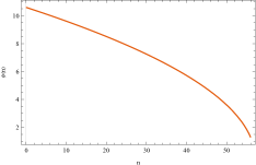
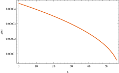
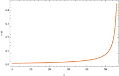
Figure 5.1: Plots of $\psi(n)$ — on the left — $\chi(n)$ — in the center — and $\epsilon(n)$ — on the right — for $0\leq n\leq 56$.

Figure 5.2 shows the same three quantities through the end of inflation (which occurs at $n_{e}\simeq 56.7$) under the assumption that the classical relations (5.36-5.38) are not corrected by the quantum effects we seek to incorporate. During this phase the inflaton oscillates around $\psi=0$ with decreasing amplitude and increasing frequency, while the first slow roll parameter oscillates in the range $0\leq\epsilon\leq 3$. Because $\epsilon={\psi^{\prime}}^{2}$, the first slow roll parameter vanishes at extrema of $\psi(n)$, and it reaches its maximum (of $\epsilon(n)=3$) when $\psi(n)=0$. Of course the dimensionless Hubble parameter is monotonically decreasing; this decrease is rapid when $\epsilon\simeq 3$, and slow when $\epsilon\simeq 0$.

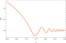
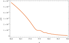
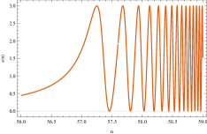
Figure 5.2: Plots of $\psi(n)$ — on the left — $\chi(n)$ — in the center — and $\epsilon(n)$ — on the right — for $56\leq n\leq 59$.

The slow roll approximation (5.46) tells us that $\psi^{\prime}\simeq-1/\psi$ and $\chi(n)\simeq c/\sqrt{3}\times\psi(n)$. Setting $D=4$, and using our values of $c=7.1\times 10^{-6}$ and $q=1.2\times 10^{-6}$, gives the mass hierarchy,

$$\frac{\mu^{2}_{u}}{\chi^{2}}\simeq 2+\frac{6q^{2}}{c^{2}}\simeq 2.16\quad>\quad\frac{\mu^{2}}{\chi^{2}}\simeq\frac{6q^{2}}{c^{2}}\simeq 0.16\quad>\quad\frac{\mu^{2}_{t}}{\chi^{2}}\simeq\frac{3}{\psi^{2}}\;.$$ (5.48)

Figure 5.3 shows the various masses through inflation.

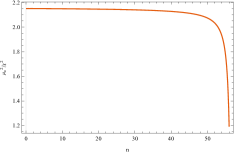
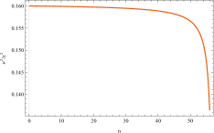
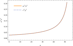
Figure 5.3: Plots of $\mu_{u}^{2}(n)/\chi^{2}(n)$ — on the left — $\mu^{2}(n)/\chi^{2}(n)$ — in the center — and $\mu^{2}_{t}(n)/\chi^{2}(n)$ — on the right — for $0\leq n\leq 56$.

As one can just see from the larger $n$ values of Figure 5.3, the hierarchy of equation (5.48) becomes inverted after the end of inflation. Figure 5.4 shows the behavior after the end of inflation. During this phase $\mu^{2}_{u}/\chi^{2}$ is mostly tachyonic, and actually diverges at points where $\psi(n)=0$. On the other hand, $\mu^{2}/\chi^{2}$ oscillates between $0$ and the small value of $0.16$, while $\mu^{2}_{t}/\chi^{2}$ grows monotonically to large, positive values. The $u$-mode mass is the most important of the three, and its evolution is the most complex. Figure 5.5 shows its behavior in more detail.

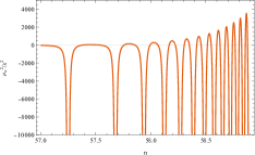
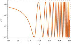
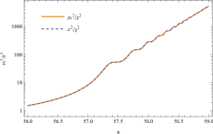
Figure 5.4: Plots of $\mu_{u}^{2}(n)/\chi^{2}(n)$ — on the left — $\mu^{2}(n)/\chi^{2}(n)$ — in the center — and $\mu^{2}_{t}(n)/\chi^{2}(n)$ — on the right — for $56\leq n\leq 59$.

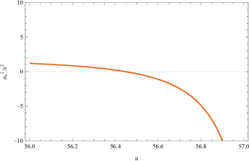
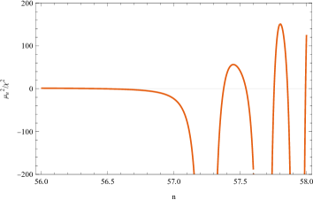
Figure 5.5: The left hand plot shows $\mu_{u}^{2}(n)/\chi^{2}(n)$ on the range $56\leq n\leq 57$, just before the first zero of $\mu(n)$. The right hand plot depicts $\mu_{u}^{2}(n)/\chi^{2}(n)$ over the slightly larger range of $56\leq n\leq 58$, which includes the first three zeroes of $\mu(n)$.

5.3.2 Approximating the Longitudinal Amplitude

Equation (5.41) for $\mathcal{T}(n,\kappa)$ contains six terms. The ultraviolet regime is defined by the condition $\kappa\gg\chi(n)e^{n}$. In this regime equation (5.41) is dominated by the 4th and 6th terms, $2\kappa^{2}e^{-2n}/\chi^{2}$ and $-e^{-2[\mathcal{T}+(D-1)n]}/2\chi^{2}$, and the amplitude takes the form,

$$\mathcal{T}(n,\kappa)=\ln\Bigl{[}\frac{1}{2\kappa}\Bigr{]}-(D\!-\!2)n$$ (5.49)

$$\hskip 76.82234pt+\Bigl{[}\frac{1}{2}(D\!-\!2)(D\!-\!2\epsilon)-\frac{2\mu_{t}^{2}}{\chi^{2}}\Bigr{]}\Bigl{(}\frac{\chi e^{n}}{2\kappa}\Bigr{)}^{2}+O\Biggl{(}\Bigl{(}\frac{\chi e^{n}}{2\kappa}\Bigr{)}^{4}\Biggr{)}\;.\qquad$$

Figure 5.6 compares numerical evolution of the exact equation (5.41) with the ultraviolet form (5.49) for wave numbers which experience first horizon crossing at $n_{1}=10$, $n_{1}=20$, and $n_{1}=30$. The agreement is excellent up to horizon crossing.

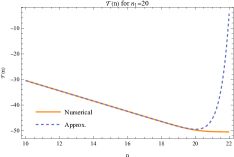
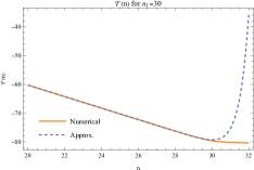
Figure 5.6: Plot comparing $\mathcal{T}(n,\kappa)$ with the ultraviolet form (5.49) for modes which experience first horizon crossing at $n_{1}=10$ (left), $n_{1}=20$ (center) and $n_{1}=30$ (right).

After 1st horizon crossing the 4th and 6th terms of (5.41) effectively drop out and the relation simplifies to,

$$\mathcal{T}^{\prime\prime}+\frac{1}{2}{\mathcal{T}^{\prime}}^{2}+(D\!-\!1\!-\!\epsilon)\mathcal{T}^{\prime}-2(D\!-\!1\!-\!\epsilon)\frac{\mu^{\prime}}{\mu}-2\frac{\mu^{\prime\prime}}{\mu}\simeq 0\;.$$ (5.50)

This is an equation for $\mathcal{T}^{\prime}$, and it is easy to see that a particular solution is,

$$\mathcal{T}^{\prime}=2\frac{\mu^{\prime}}{\mu}\;.$$ (5.51)

Integrating (5.51), and using the tensor power spectrum to infer the integration constant to all orders in the slow roll approximation [Brooker:2015iya], implies,

$$\mathcal{T}(n,\kappa)\simeq\ln\Biggl{[}\frac{\chi_{1}^{2}C(\epsilon_{1})}{2\kappa^{3}}\times\frac{\mu^{2}(n)}{\mu^{2}_{1}}\Biggr{]}\;,$$ (5.52)

where the function $C(\epsilon)$ is,

$$C(\epsilon)=\frac{1}{\pi}\Gamma^{2}\Bigl{(}\frac{1}{2}\!+\!\frac{1}{1\!-\!\epsilon}\Bigr{)}\Bigl{[}2(1\!-\!\epsilon)\Bigr{]}^{\frac{2}{1-\epsilon}}\;.$$ (5.53)

Figure 5.7 compares the exact numerical result with the infrared form (5.52) for modes which experience horizon crossing at $n_{1}=10$, $n_{1}=20$, and $n_{1}=30$. Agreement is excellent.

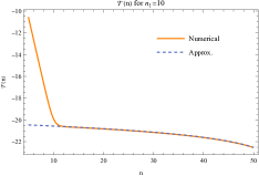
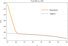
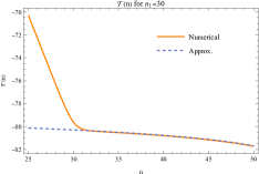
Figure 5.7: Plot comparing $\mathcal{T}(n,\kappa)$ with the late time form (5.52) for modes which experience first horizon crossing at $n_{1}=10$ (left), $n_{1}=20$ (center) and $n_{1}=30$ (right).

Although one can see from Figure 5.7 that the approximate solution (5.52) is highly accurate, it cannot be exact for two reasons:

1. We neglected the 4th and 6th terms in simplifying equation (5.41) to reach (5.50); and

2. Just because (5.51) is a solution to (5.50) does not mean it is the solution.

To find the general solution to (5.50) we substitute $\mathcal{T}^{\prime}=2\mu^{\prime}/\mu+f(n)$,

$$f^{\prime}+2\frac{\mu^{\prime}}{\mu}f+\frac{1}{2}f^{2}+(D\!-\!1\!-\!\epsilon)f\simeq 0\;.$$ (5.54)

Now divide by $\mu^{2}e^{(D-1)n}\chi f^{2}$ to reach the form,

$$\frac{\partial}{\partial n}\Biggl{[}\frac{1}{\mu^{2}e^{(D-1)n}\chi f}\Biggr{]}=\frac{1}{2\mu^{2}e^{(D-1)n}\chi}\;.$$ (5.55)

Integrating equation (5.55) from some point $n_{2}$ gives the general solution,

$$f(n)=f_{2}\Biggl{[}e^{(D-1)(n-n_{2})}\Bigl{[}\frac{\chi(n)}{\chi_{2}}\Bigr{]}\Bigl{[}\frac{\mu(n)}{\mu_{2}}\Bigr{]}^{2}$$ (5.56)

$$\hskip 113.81102pt+\frac{1}{2}f_{2}\int_{n_{2}}^{n}\!\!\!\!\!dn^{\prime}\,e^{(D-1)(n-n^{\prime})}\Bigl{[}\frac{\chi(n)}{\chi(n^{\prime})}\Bigr{]}\Bigl{[}\frac{\mu(n)}{\mu(n^{\prime})}\Bigr{]}^{2}\Biggr{]}^{-1}\;.\qquad$$

Careful consideration of (5.56) reveals that $\mathcal{T}(n,\kappa)$ actually has a finite limit as the mass vanishes. To see this, assume $n$ is such that $\mu(n)\rightarrow 0$, and expand the integral of (5.56) for small $\mu(n)$,

$$\int_{n_{2}}^{n}\!\!\!\!\!dn^{\prime}\,e^{(D-1)(n-n^{\prime})}\Bigl{[}\frac{\chi(n)}{\chi(n^{\prime})}\Bigr{]}\Bigl{[}\frac{\mu(n)}{\mu(n^{\prime})}\Bigr{]}^{2}\!\!=-\frac{\mu(n)}{\mu^{\prime}(n)}$$ (5.57)

$$\hskip 56.9055pt-\frac{1}{2}\Bigl{[}D\!-\!1\!-\!\epsilon(n)\!+\!\frac{\mu^{\prime\prime}(n)}{\mu^{\prime}(n)}\Bigr{]}\Bigl{[}\frac{\mu(n)}{\mu^{\prime}(n)}\Bigr{]}^{2}\ln[\mu^{2}(n)]+O(1)\;.\qquad$$

Near the point where $\mu(n)\rightarrow 0$ we therefore have,

$$f(n)\longrightarrow-\frac{2\mu^{\prime}(n)}{\mu(n)}+\Bigl{[}D\!-\!1\!-\!\epsilon(n)\!+\!\frac{\mu^{\prime\prime}(n)}{\mu^{\prime}(n)}\Bigr{]}\ln[\mu^{2}(n)]+O(1)\;.$$ (5.58)

Hence we have,

$$\mathcal{T}^{\prime}(n,\kappa)\longrightarrow\Bigl{[}D\!-\!1\!-\!\epsilon(n)\!+\!\frac{\mu^{\prime\prime}(n)}{\mu^{\prime}(n)}\Bigr{]}\ln[\mu^{2}(n)]+O(1)\;.$$ (5.59)

Although expression (5.59) diverges as $\mu(n)$ goes to zero, the singularity is integrable, which means that $\mathcal{T}(n,\kappa)$ remains finite.

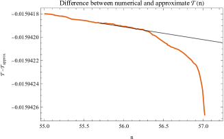
Figure 5.8: Numerical determination of the constant $f_{2}$ from the difference of $\mathcal{T}(n,\kappa)$ and expression (5.52). In this case $\kappa$ was chosen to experience first horizon crossing at $n_{1}=10$.

As we see from Figure 5.8, the constant $f_{2}$ in expression (5.56) represents the difference between the actual value of $\mathcal{T}^{\prime}(n_{2},\kappa)$ and its approximate form (5.51) $2\mu^{\prime}(n_{2})/\mu(n_{2})$. Because the approximate form is quite accurate, $f_{2}$ is a very small number, about $f_{2}\sim-10^{-7}$. The fact that $f_{2}$ drops out of the asymptotic form (5.58) means that the ultimate finiteness of $\mathcal{T}(n,\kappa)$ is a robust conclusion. However, $\mu(n)$ must be very close to zero before the integral (5.57) begins to dominate over the first term in the denominator of (5.56), which has a relative enhancement of $e^{(D-1)(n-n_{2})}$. If we take $n_{2}=56$ and define $n_{*}\simeq 57.25$ as the first zero of $\mu(n)$, the point $n_{f}$ at which expressions (5.58-5.59) become valid approximately obeys,

$$n_{*}-n_{f}\simeq\frac{1}{2}f_{2}\,e^{-3(n_{*}-n_{2})}\Bigl{(}\frac{\chi_{2}}{\chi_{*}}\Bigr{)}\Bigl{(}\frac{\mu_{2}}{\mu_{*}^{\prime}}\Bigr{)}^{2}\simeq 10^{-9}\;.$$ (5.60)

We can therefore estimate the minimum value of $\mathcal{T}(n,\kappa)$ as

$$\mathcal{T}_{\rm min}\simeq\ln\Biggl{[}\frac{\chi_{1}^{2}C(\epsilon_{1})}{2\kappa^{3}}\!\times\!\frac{1}{4}f_{2}^{2}\,e^{-6(n_{*}-n_{2})}\Bigl{(}\frac{\chi_{2}}{\chi_{*}}\Bigr{)}^{2}\Bigl{(}\frac{\mu_{2}}{\mu_{1}}\Bigr{)}^{2}\Bigl{(}\frac{\mu_{2}}{\mu_{*}^{\prime}}\Big{)}^{2}\Biggr{]}\;.$$ (5.61)

5.3.3 Approximating the Temporal Amplitude

Equation (5.42) for $\mathcal{U}(n,\kappa)$ contains the same six terms as (5.41). In the ultraviolet it is also dominated by the 4th and 6th terms, $2\kappa^{2}e^{-2n}/\chi^{2}$ and $-e^{-2[\mathcal{U}+(D-1)n]}/2\chi^{2}$. Hence the ultraviolet expansion of $\mathcal{U}(n,\kappa)$ takes the same form as (5.49),

$$\mathcal{U}(n,\kappa)=\ln\Bigl{[}\frac{1}{2\kappa}\Bigr{]}-(D\!-\!2)n$$ (5.62)

$$\hskip 76.82234pt+\Bigl{[}\frac{1}{2}(D\!-\!2)(D\!-\!2\epsilon)-\frac{2\mu_{u}^{2}}{\chi^{2}}\Bigr{]}\Bigl{(}\frac{\chi e^{n}}{2\kappa}\Bigr{)}^{2}+O\Biggl{(}\Bigl{(}\frac{\chi e^{n}}{2\kappa}\Bigr{)}^{4}\Biggr{)}\;.\qquad$$

Figure 5.9 compares the exact numerical solution with the ultraviolet form (5.62) for modes which experience first horizon crossing at $n_{1}=10$, $n_{1}=20$ and $n_{1}=30$. Agreement is excellent up to first horizon crossing, just as it was in the analogous comparison of Figure 5.6 for $\mathcal{T}(n,\kappa)$.

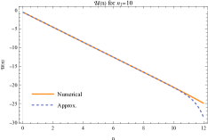
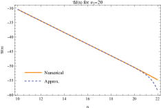
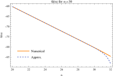
Figure 5.9: Plot comparing $\mathcal{U}(n,\kappa)$ with the ultraviolet form (5.62) for modes which experience first horizon crossing at $n_{1}=10$ (left), $n_{1}=20$ (center) and $n_{1}=30$ (right).

The 4th and 6th terms of (5.42) drop out after first horizon crossing, and the relation simplifies to,

$$\mathcal{U}^{\prime\prime}+\frac{1}{2}{\mathcal{U}^{\prime}}^{2}+(D\!-\!1\!-\!\epsilon)\mathcal{U}^{\prime}+\frac{2\mu^{2}_{u}}{\chi^{2}}\simeq 0\;.$$ (5.63)

Recall from Figure 5.3 that $\mu_{u}^{2}(n)/\chi^{2}(n)$ is approximately constant during inflation. This means that equation (5.63) can be roughly solved as,

$$\mathcal{U}^{\prime}(n,\kappa)\simeq-(D\!-\!1\!-\!\epsilon)+\sqrt{(D\!-\!1\!-\!\epsilon)^{2}-\frac{4\mu_{u}^{2}}{\chi^{2}}}\;.$$ (5.64)

With the appropriate integration constant we therefore have,

$$\mathcal{U}(n,\kappa)\simeq\ln\Biggl{[}\frac{\chi_{1}^{2}C(\epsilon_{1})}{2\kappa^{3}}\!\times\!\frac{\chi_{1}}{\chi(n)}\Biggl{]}-(D\!-\!1)(n\!-\!n_{1})$$ (5.65)

$$\hskip 142.26378pt+\int_{n_{1}}^{n}\!\!\!\!dn^{\prime}\sqrt{[D\!-\!1\!-\!\epsilon(n^{\prime})]^{2}-\frac{4\mu_{u}^{2}(n^{\prime})}{\chi^{2}(n^{\prime})}}\;.\qquad$$

Figure 5.10 compares this approximation with the numerical evolution for modes which experience horizon crossing at $n_{1}=10$, $n_{1}=20$ and $n_{1}=30$.

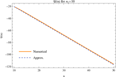
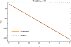
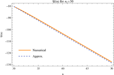
Figure 5.10: Plot comparing $\mathcal{U}(n,\kappa)$ with the late time form (5.65) for modes which experience first horizon crossing at $n_{1}=10$ (left), $n_{1}=20$ (center) and $n_{1}=30$ (right).

After the end of inflation $\mu^{2}(n)/\chi^{2}(n)$ falls off whereas the derivative terms in $\mu^{2}_{u}/\chi^{2}$ become large and tachyonic. This means we can neglect $\mu^{2}(n)/\chi^{2}(n)$,

$$\frac{\mu_{u}^{2}}{\chi^{2}}\simeq(D\!-\!2)(1\!-\!\epsilon)-(D\!-\!3\!+\!\epsilon)\frac{\mu^{\prime}}{\mu}+\Bigl{(}\frac{\mu^{\prime}}{\mu}\Bigr{)}^{\prime}-\Bigl{(}\frac{\mu^{\prime}}{\mu}\Bigr{)}^{2}\;.$$ (5.66)

We now make the substitution,

$$\mathcal{U}^{\prime}(n,\kappa)=-\frac{2\mu^{\prime}(n)}{\mu(n)}-2(D\!-\!2)+g(n)\;,$$ (5.67)

in equation (5.63) to find,

$$g^{\prime}-\Bigl{(}D\!-\!3\!+\!\epsilon\!+\!2\frac{\mu^{\prime}}{\mu}\Bigr{)}g+\frac{1}{2}g^{2}=0\;.$$ (5.68)

Multiplying by $e^{(D-3)n}\mu^{2}(n)/[\chi(n)g^{2}(n)]$ makes the $g$-dependent terms a total derivative, and permits us to write the general solution as,

$$g(n)=g_{2}\Biggl{[}e^{-(D-3)(n-n_{2})}\Bigl{[}\frac{\chi(n)}{\chi_{2}}\Bigr{]}\Bigl{[}\frac{\mu_{2}}{\mu(n)}\Bigr{]}^{2}$$ (5.69)

$$\hskip 113.81102pt+\frac{1}{2}g_{2}\!\!\int_{n_{2}}^{n}\!\!\!\!\!dn^{\prime}\,e^{-(D-3)(n-n^{\prime})}\Bigl{[}\frac{\chi(n)}{\chi(n^{\prime})}\Bigr{]}\Bigl{[}\frac{\mu(n^{\prime})}{\mu(n)}\Bigr{]}^{2}\Biggr{]}^{-1}\;,\qquad$$

where the constant $g_{2}$ is determined to interpolate between (5.64) and (5.67),

$$g_{2}=\frac{2\mu_{2}^{\prime}}{\mu_{2}}+(D\!-\!3\!+\!\epsilon_{2})+\sqrt{(D\!-\!1\!-\!\epsilon_{2})^{2}-\frac{4\mu_{2}^{2}}{\chi_{2}^{2}}}\;.$$ (5.70)

Note that, whereas $f(n)$ diverges as $\mu(n)$ approaches zero, $g(n)$ goes to zero like $\mu^{2}(n)$.

Integrating equation (5.67), and using (5.65) to supply the integration constant, gives,

$$\mathcal{U}(n,\kappa)\simeq\ln\Biggl{[}\frac{\chi_{1}^{2}C(\epsilon_{1})}{2\kappa^{3}}\!\times\!\frac{\chi_{1}}{\chi_{2}}\!\times\!\frac{\mu_{2}^{2}}{\mu^{2}(n)}\Biggr{]}-(D\!-\!1)(n_{2}\!-\!n_{1})-2(D\!-\!2)(n\!-\!n_{2})$$ (5.71)

$$\hskip 91.04872pt+\int_{n_{1}}^{n_{2}}\!\!\!\!\!dn^{\prime}\sqrt{[D\!-\!1\!-\!\epsilon(n^{\prime})]^{2}-\frac{4\mu_{u}^{2}(n^{\prime})}{\chi^{2}(n^{\prime})}}+\int_{n_{2}}^{n}\!\!\!\!\!dn^{\prime}\,g(n^{\prime})\;.\qquad$$

Because $g(n)$ vanishes as $\mu(n)\rightarrow 0$, the $-\ln[\mu^{2}(n)]$ divergence of $\mathcal{U}(n,\kappa)$ is robust. Note that this is not even affected by neglecting $\mu^{2}(n)/\chi^{2}(n)$ in (5.66). Figure 5.11 compares the numerical solution with our analytic approximation (5.71).

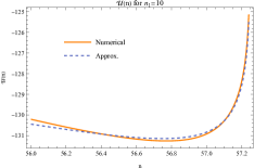
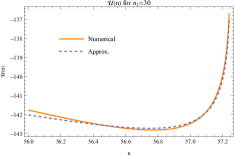
Figure 5.11: Plot comparing $\mathcal{U}(n,\kappa)$ with the post-inflationary form (5.71) for modes which experience first horizon crossing at $n_{1}=10$ (left), $n_{1}=20$ (center) and $n_{1}=30$ (right).

5.4 Quantum-Correcting the Inflaton 0-Mode

The purpose of this section is to use the photon propagator to quantum-correct the classical equation for the inflaton $0$-mode from (5.15) to,

$$\partial_{0}\Bigl{[}a^{D-2}\partial_{0}\varphi_{0}\Bigr{]}+a^{D}\varphi_{0}V^{\prime}(\varphi_{0}^{2})+q^{2}\varphi_{0}a^{D-2}\eta^{\mu\nu}i\Bigl{[}\mbox{}_{\mu}\Delta_{\nu}\Bigr{]}(x;x)=0\;.$$ (5.72)

We begin by deriving exact expressions for the $t$-mode and $u$-mode contributions to trace of the photon propagator. We then use a variant of the work-energy theorem to show how reheating occurs.

5.4.1 The Effective Force

The $t$-mode contribution to the coincidence limit of the trace of the photon propagator in equation (5.72) is,

$$\sqrt{-g}\,g^{\mu\nu}i\Bigl{[}\mbox{}_{\mu}\Delta_{\nu}\Bigr{]}_{t}(x;x)=a^{D-2}\!\!\int\!\!\frac{d^{D-1}k}{(2\pi)^{D-1}}\Biggl{\{}\frac{1}{M^{2}}\,\widehat{\partial}_{0}t\!\cdot\!\widehat{\partial_{0}}t^{*}-\frac{k^{2}}{M^{2}}\,t\!\cdot\!t^{*}\Biggr{\}}\;.$$ (5.73)

The $t$-mode equation (5.27) can be exploited to write the product of time derivatives in terms of the norm-squared,

$$\partial_{0}t\!\cdot\!\partial_{0}t^{*}=\Bigl{[}\frac{1}{2}\partial_{0}^{2}+\frac{1}{2}(D\!-\!2)aH\partial_{0}+k^{2}-(D\!-\!2)aH\frac{\partial_{0}M}{M}-\frac{\partial_{0}^{2}M}{M}\Bigr{]}(tt^{*})\;.$$ (5.74)

Using this identity we can re-express the $t$-mode contribution (5.73) as,

$$\sqrt{-g}\,g^{\mu\nu}i\Bigl{[}\mbox{}_{\mu}\Delta_{\nu}\Bigr{]}_{t}=\frac{a^{D-2}}{M^{2}}\!\!\int\!\!\frac{d^{D-1}k}{(2\pi)^{D-1}}\Biggl{\{}\frac{1}{2}\partial_{0}^{2}+\frac{1}{2}(D\!-\!2)aH\partial_{0}-\frac{\partial_{0}M}{M}\partial_{0}$$ (5.75)

$$\hskip 113.81102pt-(D\!-\!2)aH\frac{\partial_{0}M}{M}-\frac{\partial_{0}^{2}M}{M}+\Bigl{(}\frac{\partial_{0}M}{M}\Bigr{)}^{2}\Biggr{\}}(tt^{*})\;.\qquad$$

Converting to dimensionless form, and employing equation (5.41) to eliminate second derivatives, gives the compact form,

$$\sqrt{-g}\,g^{\mu\nu}i\Bigl{[}\mbox{}_{\mu}\Delta_{\nu}\Bigr{]}_{t}(x;x)=\frac{e^{Dn}\chi^{2}(n)}{(8\pi G)^{\frac{D}{2}-1}\mu^{2}(n)}\!\!\int\!\!\frac{d^{D-1}\kappa}{(2\pi)^{D-1}}\,e^{\mathcal{T}(n,\kappa)}$$ (5.76)

$$\hskip 36.98866pt\times\Biggl{\{}\Bigl{[}\frac{1}{2}\mathcal{T}^{\prime}(n,\kappa)-\frac{\mu^{\prime}(n)}{\mu(n)}\Bigr{]}^{2}-\frac{\kappa^{2}e^{-2n}}{\chi^{2}(n)}+\frac{1}{4\chi^{2}}e^{-2[\mathcal{T}(n,\kappa)+(D-1)n]}\Biggr{\}}.\qquad$$

The $u$-mode contribution to the photon trace in (5.72) is,

$$\sqrt{-g}\,g^{\mu\nu}i\Bigl{[}\mbox{}_{\mu}\Delta_{\nu}\Bigr{]}_{u}(x;x)=a^{D-2}\!\!\int\!\!\frac{d^{D-1}k}{(2\pi)^{D-1}}\Biggl{\{}-\frac{k^{2}}{M^{2}}\,u\!\cdot\!u^{*}+\frac{1}{M^{2}}\widetilde{D}u\!\cdot\!\widetilde{D}u^{*}\Biggr{\}}\;.$$ (5.77)

We can eliminate the norm-square of $\partial_{0}u$ using the $u$-mode equation (5.29),

$$\partial_{0}u\!\cdot\!\partial_{0}u^{*}=\Biggl{[}\frac{1}{2}\partial_{0}^{2}+\frac{1}{2}(D\!-\!2)aH\partial_{0}+k^{2}+a^{2}M^{2}+(D\!-\!2)a^{2}H^{2}(1\!-\!\epsilon)$$ (5.78)

$$\hskip 91.04872pt-(D\!-\!2)aH\frac{\partial_{0}M}{M}+\partial_{0}\Bigl{(}\frac{\partial_{0}M}{M}\Bigr{)}-\Bigl{(}\frac{\partial_{0}M}{M}\Bigr{)}^{2}\Biggr{]}(uu^{*})\;.\qquad$$

Substituting (5.78) in (5.77), and taking apart the factors of $\widetilde{D}=\partial_{0}+(D-2)aH+\partial_{0}M/M$ gives,

$$\sqrt{-g}\,g^{\mu\nu}i\Bigl{[}\mbox{}_{\mu}\Delta_{\nu}\Bigr{]}_{u}=\frac{a^{D-2}}{M^{2}}\!\!\int\!\!\frac{d^{D-1}k}{(2\pi)^{D-1}}\Biggl{\{}\frac{1}{2}\partial_{0}^{2}+\frac{3}{2}(D\!-\!2)aH\partial_{0}+\frac{\partial_{0}M}{M}\partial_{0}+a^{2}M^{2}$$ (5.79)

$$\hskip 19.91684pt+(D\!-\!2)(D\!-\!1\!-\!\epsilon)a^{2}H^{2}+(D\!-\!2)aH\frac{\partial_{0}M}{M}+\partial_{0}\Bigl{(}\frac{\partial_{0}M}{M}\Bigr{)}\Biggr{\}}(uu^{*})\;.\qquad$$

The final, dimensionless form is very similar to (5.76),

$$\sqrt{-g}\,g^{\mu\nu}i\Bigl{[}\mbox{}_{\mu}\Delta_{\nu}\Bigr{]}_{u}(x;x)=\frac{e^{Dn}\chi^{2}(n)}{(8\pi G)^{\frac{D}{2}-1}\mu^{2}(n)}\!\!\int\!\!\frac{d^{D-1}\kappa}{(2\pi)^{D-1}}\,e^{\mathcal{U}(n,\kappa)}$$ (5.80)

$$\times\Biggl{\{}\Bigl{[}\frac{1}{2}\mathcal{U}^{\prime}(n,\kappa)+\frac{\mu^{\prime}(n)}{\mu(n)}+D\!-\!2\Bigr{]}^{2}-\frac{\kappa^{2}e^{-2n}}{\chi^{2}(n)}+\frac{1}{4\chi^{2}}e^{-2[\mathcal{U}(n,\kappa)+(D-1)n]}\Biggr{\}}.\qquad$$

5.4.2 Reheating

The dimensionless form of the inflaton $0$-mode equation (5.72) takes the form,

$$e^{n}\chi\frac{\partial}{\partial n}\Bigl{[}e^{(D-1)n}\chi\psi^{\prime}\Bigr{]}=-e^{Dn}\psi\Biggl{[}U^{\prime}(\psi^{2})+\frac{Q^{2}\chi^{2}}{\mu^{2}}\!\!\int\!\!\frac{d^{D-1}\kappa}{(2\pi)^{D-1}}\Biggl{\{}\qquad\Biggr{\}}\Biggr{]}\equiv\mathcal{F}\;.$$ (5.81)

where the term inside the curly brackets is the sum of the $t$ and $u$ contributions from expressions (5.76) and (5.80), and $Q^{2}\equiv q^{2}/(8\pi G)^{\frac{D}{2}-2}$ is the dimensionless charge. Multiplying both sides of (5.81) by $e^{(D-2)n}\chi\psi^{\prime}$ and integrating gives a curious generalization of the famous work-energy theorem of introductory physics,

$$e^{(D-1)n}\chi\psi^{\prime}\frac{\partial}{\partial n}\Bigl{[}e^{(D-1)n}\chi\psi^{\prime}\Bigr{]}=\frac{1}{2}\frac{\partial}{\partial n}\Bigl{[}e^{(D-1)n}\chi\psi^{\prime}\Bigr{]}^{2}=e^{(D-2)n}\chi\psi^{\prime}\!\times\!\mathcal{F}\;.$$ (5.82)

We now integrate (5.82) from the beginning of reheating (at $n=n_{i}$) to the end (at $n=n_{f}$), and use the fact that $\psi^{\prime}(n_{f})=0$ at the end of reheating,

$$0-\frac{1}{2}\Bigl{[}e^{(D-1)n_{i}}\chi_{i}\psi^{\prime}_{i}\Bigr{]}^{2}=\int_{n_{i}}^{n_{f}}\!\!\!\!dn\,e^{(D-2)n}\chi(n)\psi^{\prime}(n)\mathcal{F}(n)\;.$$ (5.83)

Equation (5.83) clearly implies that the product of $\psi^{\prime}(n)\times\mathcal{F}(n)$ must be negative in order to suck the energy out of the inflaton $0$-mode. The classical contribution from $\psi^{\prime}\times-\psi U^{\prime}(\psi^{2})$ is positive, so reheating must be driven by the quantum corrections from the $t$-modes and the $u$-modes, each of which has two positive and one negative contribution. From expressions (5.76) and (5.80) we see that the desired negative contribution can only come from the $-\kappa^{2}e^{-2n}/\chi^{2}(n)$ terms, however, it is not clear if the dominant effect comes from $t$-modes or $u$-modes. It is also not clear whether the largest contributions come from super-horizon modes (with $\kappa<\chi(n_{e})e^{n_{e}}$, where $n_{e}$ denotes the end of inflation) or sub-horizon modes (with $\kappa>\chi(n_{e})e^{n_{e}}$). Note that discretization can only recover the longest wavelength sub-horizon modes.

Let us first examine sub-horizon modes, for which $\chi e^{n}/\kappa$ is small. In this case the ultraviolet expansions (5.49) and (5.62) imply that the multiplicative exponentials agree to leading order,

$$e^{\mathcal{T}(n,\kappa)}=\frac{e^{-(D-2)n}}{2\kappa}\Biggl{\{}1+O\Bigl{(}\frac{\chi^{2}e^{2n}}{\kappa^{2}}\Bigr{)}\Biggr{\}}\;\;,\;\;e^{\mathcal{U}(n,\kappa)}=\frac{e^{-(D-2)n}}{2\kappa}\Biggl{\{}1+O\Bigl{(}\frac{\chi^{2}e^{2n}}{\kappa^{2}}\Bigr{)}\Biggr{\}}\;.$$ (5.84)

Substituting the same ultraviolet expansions into the curly bracketed parts of (5.76) and (5.80) gives,

$$\Bigl{[}\frac{1}{2}\mathcal{T}^{\prime}-\frac{\mu^{\prime}}{\mu}\Bigr{]}^{2}-\frac{\kappa^{2}e^{-2n}}{\chi^{2}}+\frac{e^{-2[\mathcal{T}+(D-1)n]}}{4\chi^{2}}$$ (5.85)

$$\hskip 56.9055pt=-\frac{1}{2}(D\!-\!2)(1\!-\!\epsilon)-(1\!-\!\epsilon)\frac{\mu^{\prime}}{\mu}-\Bigl{(}\frac{\mu^{\prime}}{\mu}\Bigr{)}^{\prime}+O\Bigl{(}\frac{\chi^{2}e^{2n}}{\kappa^{2}}\Bigr{)}\;,\qquad$$

$$\Bigl{[}\frac{1}{2}\mathcal{U}^{\prime}+\frac{\mu^{\prime}}{\mu}+D\!-\!2\Bigr{]}^{2}-\frac{\kappa^{2}e^{-2n}}{\chi^{2}}+\frac{e^{-2[\mathcal{U}+(D-1)n]}}{4\chi^{2}}$$ (5.86)

$$\hskip 56.9055pt=\frac{1}{2}(D\!-\!2)(1\!-\!\epsilon)+(1\!-\!\epsilon)\frac{\mu^{\prime}}{\mu}+\Bigl{(}\frac{\mu^{\prime}}{\mu}\Bigr{)}^{\prime}+O\Bigl{(}\frac{\chi^{2}e^{2n}}{\kappa^{2}}\Bigr{)}\;.\qquad$$

Hence there is perfect cancellation between the sub-horizon $t$-mode and $u$-mode contributions at leading order.

Super-horizon modes cannot show the same cancellation because $\mathcal{T}(n,\kappa)$ approaches a large, negative constant (5.61) as $\mu(n)$ goes to zero, whereas $\mathcal{U}(n,\kappa)$ diverges like $\mathcal{U}_{*}+\ln[\mu_{2}^{2}/\mu^{2}(n)]$. This means that the multiplicative exponentials take the form,

$$e^{\mathcal{T}(n,\kappa)}\longrightarrow e^{\mathcal{T}_{\rm min}}\qquad,\qquad e^{\mathcal{U}(n,\kappa)}\longrightarrow e^{\mathcal{U}_{*}}\Bigl{[}\frac{\mu_{2}}{\mu(n)}\Bigr{]}^{2}\;.$$ (5.87)

The curly bracketed terms which involve explicit factors of $\mu^{\prime}/\mu$ wind up depending on the functions $f(n)$ and $g(n)$, given in expressions (5.56) and (5.69), respectively,

$$\Bigl{[}\frac{1}{2}\mathcal{T}^{\prime}-\frac{\mu^{\prime}}{\mu}\Bigr{]}^{2} \!\!\!=\!\!\! \frac{1}{4}f^{2}(n)\longrightarrow\Bigl{[}\frac{\mu^{\prime}(n)}{\mu(n)}\Bigr{]}^{2}\;,$$ (5.88)

$$\Bigl{[}\frac{1}{2}\mathcal{U}^{\prime}+\frac{\mu^{\prime}}{\mu}+D\!-\!2\Bigr{]}^{2} \!\!\!=\!\!\! \frac{1}{4}g^{2}(n)\longrightarrow 0\;.$$ (5.89)

This means that the $t$-modes contribute positively, while the $u$-modes make a negative contribution,

$$e^{\mathcal{T}}\!\times\!\Biggl{\{}\qquad\Biggr{\}} \!\!\!\longrightarrow\!\!\! e^{\mathcal{T}_{\rm min}}\Bigl{[}\frac{\mu^{\prime}(n)}{\mu(n)}\Bigr{]}^{2}\;,$$ (5.90)

$$e^{\mathcal{U}}\!\times\!\Biggl{\{}\qquad\Biggr{\}} \!\!\!\longrightarrow\!\!\! e^{\mathcal{U}_{*}}\Bigl{[}\frac{\mu_{2}}{\mu(n)}\Bigr{]}^{2}\!\times\!-\frac{\kappa^{2}e^{-2n_{*}}}{\chi_{*}^{2}}\;.\qquad$$ (5.91)

How large the relative coefficients are depends on the integration constant $f_{2}$, for which we do not yet have an analytic form.

Whether (5.90) or (5.91) dominates, it is significant that both terms diverge like $1/\mu^{2}(n)$. Because the effective force contains another factor of $1/\mu^{2}(n)$, this means that the quantum correction diverges like $1/\mu^{4}(n)$ near the point $n_{*}$ at which $\mu(n)$ vanishes. The measure factor in (5.83) softens this somewhat, but not enough,

$$Q^{2}\psi^{\prime}(n)\psi(n)dn=\frac{1}{4}d\mu^{2}\;.$$ (5.92)

The integral (5.83) therefore diverges before $\mu(n)=0$, which presumably brings reheating to an end.

5.5 Conclusions

Ema et al. have shown that coupling a charged inflaton to electromagnetism provides the most efficient reheating [Ema:2016dny]. The mechanism is that the inflaton’s evolution induces a time-dependent photon mass through the Higgs mechanism. Nothing special changes about the transverse spatial polarizations, but inverse powers of the mass appear in the longitudinal-temporal polarizations (5.26) and (5.28), which result from the photon having “eaten” the phase of the inflaton field. These factors diverge when the inflaton passes through zero. The effect is strengthened by factors of $\mu^{\prime}(n)/\mu(n)$ which appear in the mass terms (5.43-5.44) of the two modes.

This chapter represents an effort to improve on previous excellent numerical studies of this process based on discretizing space [Bezrukov:2020txg]. Although that method can accommodate arbitrarily strong photon fields, it is of course limited to a finite range of sub-horizon modes. In contrast, we use the trace of the coincident photon propagator to study the inflaton $0$-mode equation (5.72). Our expressions (5.75-5.76) and (5.79-5.80) for the longitudinal and temporal contributions to this trace are exact. They can be used to include the effects of super-horizon modes, and of arbitrarily short wave length modes. In fact, our use of dimensional regularization means that the far ultraviolet can be included as well, through the use of expansions (5.49) and (5.62).

We have also derived good analytic approximations for the amplitudes. Before first horizon crossing these are (5.49) and (5.62), respectively. After first crossing the $t$-mode amplitude is well approximated by expression (5.52) until close to the point at which $\mu(n)=0$. However, expression (5.59) shows that the $t$-mode amplitude remains finite when $\mu(n)=0$.

Two forms are required to approximate the $u$-mode amplitude after first horizon crossing, owing to its dependence on the complicated behavior of the $u$-mode mass term (5.44), which is evident from Figures 5.4 and 5.5. During inflation, the near constancy of $\epsilon(n)$ and $\mu^{2}_{u}(n)/\chi^{2}(n)$, result in expression (5.65) giving a good approximation. After the end of inflation the better approximation is provided by expression (5.71). Because this last form becomes exact as $\mu(n)\rightarrow 0$, we know that the $u$-mode amplitude diverges like $-\ln[\mu^{2}(n)]$, which provides an extra factor of $1/\mu^{2}(n)$ in the trace of the photon propagator (5.80).

The obvious next step is to exploit the powerful analytic expressions we have derived to make a detailed numerical study of reheating in a realistic model, such as Starobinsky inflation [Starobinsky:1980te], Higgs inflation [Bezrukov:2007ep], or a hybrid model [Bezrukov:2020txg]. Such an analysis would begin by renormalizing equation (5.72), and then focus on determining whether the dominant effect for $\mu(n)\rightarrow 0$ comes from sub-horizon or super-horizon modes, and whether it is the $t$-modes or the $u$-modes which contribute more strongly. Another key issue is whether or not the effect is so strong that the inflaton is precluded from making even a single oscillation. Right now, it seems as if the strongest effect comes from super-horizon $u$-modes, and this contribution is so strong that the inflaton $0$-mode is prevented from passing through zero.

Finally, our extension of the vector propagator to include time-dependent masses in cosmological backgrounds has two obvious applications in addition to reheating. The first of these is the study of quantum corrections to the expansion history of classical inflation [Miao:2015oba, Liao:2018sci, Kyriazis:2019xgj, Miao:2019bnq, Miao:2020zeh, Sivasankaran:2020dzp, Katuwal:2021kry]. Another obvious application is for the study of phase transitions in the early universe [Ema:2016dny].

Chapter 6 SUMMARY AND CONCLUSIONS

In this dissertation, we considered various aspects of perturbative quantum gravity and its application to early universe cosmology.

After an introduction, in Chapter 2, we considered quantum gravitational corrections to Maxwell’s equations on flat space background. Although the vacuum polarization is highly gauge dependent, we explicitly showed that this gauge dependence is canceled by contributions from the source which disturbs the effective field and the observer who measures it. Our final result is a gauge independent, real and causal effective field equation that can be used in the same way as the classical Maxwell equation.

In Chapter 3, we discussed how physicists working on atom interferometers are interested in scalar couplings to electromagnetism of dimensions 5 and 6 which might be induced by quantum gravity. There is a widespread belief that such couplings can only be induced by conjectured non-perturbative effects, resulting in unknown coupling strengths. However, we exhibited a completely perturbative mechanism through which quantum gravity induces dimension six couplings with precisely calculable coefficients.

Next, in Chapter 4, we accurately approximated the contribution that photons make to the effective potential of a charged inflaton for inflationary geometries with an arbitrary first slow roll parameter $\epsilon$. We found a small, nonlocal contribution and a numerically larger, local part. The local part involves first and second derivatives of $\epsilon$, coming exclusively from the constrained part of the electromagnetic field which carries the long range interaction. This causes the effective potential induced by electromagnetism to respond more strongly to geometrical evolution than for either scalars, which have no derivatives, or spin one half particles, which have only one derivative. For $\epsilon=0$ our final result agreed with that of Allen on de Sitter background[Allen:1983dg], while the flat space limit agrees with the classic result of Coleman and Weinberg[Coleman:1973jx].

Finally, in Chapter 5 we considered reheating for a charged inflaton which is minimally coupled to electromagnetism. The evolution of such an inflaton induces a time-dependent mass for the photon. We showed how the massive photon propagator can be expressed as a spatial Fourier mode sum involving three different sorts of mode functions, just like the constant mass case in Chapter 4. We developed accurate analytic approximations for these mode functions, and used them to approximate the effective force exerted on the inflaton 0-mode. This effective force allows one to simply compute the evolution of the inflaton 0-mode and to follow the progress of reheating.