Increasing the power of survey data with multipole-based intrinsic alignment estimators

Abstract

It has long been known that galaxy shapes align coherently with the large-scale density field. Characterizing this effect is essential to interpreting measurements of weak gravitational lensing, the deflection of light from distant galaxies by matter overdensities along the line of sight, as it produces coherent galaxy alignments that we wish to interpret in terms of a cosmological model. Existing direct measurements of intrinsic alignments using galaxy samples with high-quality shape and redshift measurements typically use well-understood but sub-optimal projected estimators, which do not make good use of the information in the data when comparing those estimators to theoretical models. We demonstrate a more optimal estimator, based on a multipole expansion of the correlation functions or power spectra, for direct measurements of galaxy intrinsic alignments. We show that even using the lowest order multipole alone increases the significance of inferred model parameters using simulated and real data, without any additional modeling complexity. We apply this estimator to measurements of intrinsic alignments in the Sloan Digital Sky survey, demonstrating consistent results with a factor of $\sim$2 greater precision in parameter fits to intrinsic alignments models. This result is functionally equivalent to quadrupling the survey area, but without the attendant costs – thereby demonstrating the value in using this new estimator in current and future intrinsic alignments measurements using spectroscopic galaxy samples.

1 Introduction

Weak gravitational lensing, the deflection of light rays from distant galaxies due to the gravitational potential of intervening matter, is among the most promising ways to stress test and constrain the parameters of our current cosmological model (Weinberg et al., 2013; Kilbinger, 2015). In recent years, weak lensing has been used to constrain the amplitude of structure growth and its evolution with a precision of 3–5 per cent (Amon et al., 2022; Secco et al., 2022; van den Busch et al., 2022; Dalal et al., 2023; Li et al., 2023). Upcoming surveys such as Euclid (Laureijs et al., 2011), the Vera C. Rubin Observatory Legacy Survey of Space and Time (Ivezić et al., 2019), and the Nancy Grace Roman Space Telescope High Latitude Imaging Survey (Akeson et al., 2019) have been formulated with a goal of increasingly ambitious weak lensing measurements to enable precise cosmological measurements.

With increasing statistical constraining power, characterizing and mitigating sources of systematic uncertainty in weak lensing (Mandelbaum et al., 2018) is increasingly a priority. Since measuring weak lensing relies on measuring coherent galaxy alignments, any alignments not due to lensing must be either removed or modeled. One such source of coherent alignments other than lensing are intrinsic alignments (Joachimi et al., 2015; Troxel & Ishak, 2015), the coherent alignment of galaxy shapes due to physically localized effects such as tidal fields generated by the large-scale structure. Since the first detections of large-scale alignments of galaxy shapes with overdensities (Mandelbaum et al., 2006; Hirata et al., 2007), the field has expanded to include a wide range of measurement and modeling efforts. Direct measurement of intrinsic alignments using galaxy samples with spectroscopic or high-quality photometric redshifts, and with galaxy shape estimates, is of particularly high value as it provides a direct empirical constraint on the amplitude and scale-dependence of these alignments, and their dependence on galaxy properties (for recent constraints, see for example Johnston et al., 2019; Fortuna et al., 2021b; Samuroff et al., 2022).

Two major challenges in direct measurement of alignments is in the quantity and type of data available to carry them out. Current direct alignment measurements are dominated by the noise from the random component of galaxy shapes, and typically can constrain the alignments over tens of Mpc at the $\sim$10 per cent level. Procuring larger samples with both robust shape and spectroscopic measurements is quite challenging given the cost of the latter, imposing a practical limitation on the size of available datasets and on the increase in precision that may be achieved through larger datasets. Another challenge relates to the fact that the existing samples are typically brighter than those used for weak lensing measurements, introducing some systematic uncertainty in extrapolating the trends found in direct measurements to the samples used for weak lensing measurements.

Given limitations in the sizes of suitable datasets, and a desire to split existing samples by properties such as luminosity and color to more deeply understand variations in alignment with these quantities, a natural question is how to make and interpret the measurements in a way that optimally extracts information from them. Many of those measurements have used 2D projected correlation functions in order to reduce the burden of modeling redshift-space distortions and other sources of complexity, though a few have used other statistics (e.g., Okumura et al., 2009). Carrying out the projected correlation function measurement involves measuring density-shape correlations as a function of both projected separation $r_{\mathrm{p}}$ and line-of-sight separation $\Pi$, then integrating along some range of $\Pi$ values. However, Singh & Mandelbaum (2016) showed that basic geometric considerations lead to a well-defined scaling of the alignment signal in the $(r_{\mathrm{p}},\Pi)$ plane, and this opens up the possibility of a more optimal matched filter approach with a multipole expansion in that plane (see also Okumura et al., 2020). Doing so has the potential to not only increase the statistical significance of intrinsic alignment model constraints and trends with galaxy properties, but also to improve our ability to constrain the intrinsic alignment model on intermediate scales where we expect behavior that requires more complex modeling efforts (e.g., Blazek et al., 2015; Vlah et al., 2020; Fortuna et al., 2021a).

The goal of this work, therefore, is to demonstrate an improved intrinsic alignment estimator that increases the statistical precision of intrinsic alignment model constraints. We quantify the efficacy of this estimator using simulated data along with a re-analysis of data from the Sloan Digital Sky Survey (SDSS).

The outline of this work is as follows. In Sec. 2, we present the formalism used to describe intrinsic alignments and to connect our estimators to theory. Next, we describe the simulated and real datasets used in this work in Sec. 3. Our measurement methods are described in Sec. 4 Sec. 5 shows our results, and we discuss them and their implications for future intrinsic alignments measurements in Sec. 6.

2 Formalism

In this section we describe the theoretical formalism for the models and estimators used. We will closely follow the notation of Singh et al. (2015, 2021).

To model the intrinsic alignments of galaxies, we will use the linear alignment model (Catelan et al., 2001; Hirata & Seljak, 2003). The linear alignment model states that the intrinsic shapes of galaxies are correlated with the initial tidal field at the time of the formation of galaxies. As a result, the correlated shear in the intrinsic galaxy shapes can be written as:

$$\gamma^{I}=(\gamma^{I}_{+},\gamma^{I}_{\times})=-\frac{C_{1}}{4\pi G}(\partial^{2}_{x}-\partial^{2}_{y},\partial_{x}\partial_{y})\phi_{p},$$ (1)

where $\gamma^{I}$ is the intrinsic shear with two components $\gamma^{I}_{+},\gamma^{I}_{\times}$, $\phi_{p}$ is the gravitational potential at the time of galaxy formation, $C_{1}$ is an unknown constant encapsulating the strength of the linear response of galaxy shapes to the tidal fields. Later in this section, when defining the power spectra of galaxy shapes, we will use the non-linear matter power spectra instead of the linear matter power spectra as expected from the linear alignment model (a modification that was proposed by Hirata & Seljak 2003 and implemented by Bridle & King 2007). The resultant model is called the non-linear alignment model (NLA).

2.1 Power spectra and Correlation functions

The correlations among different cosmological observables are typically measured and quantified using the power spectrum or its Fourier counterpart, the two-point correlation function. To study the intrinsic alignments of galaxy shapes, we measure the auto- and cross-correlations between the galaxy positions and their shapes, quantifying the statistical tendency for galaxy shapes to point towards nearby overdensities. For these measurements, the galaxy samples used for tracing the galaxy density field and the intrinsic shear field (IA) can in general be different. In this paper, we will denote the quantities associated with the density tracer sample with subscript $D$ and for the sample with shape measurements as $S$.

In the linear alignment model, the auto- and cross-power spectra between galaxies and shapes are given as (Hirata & Seljak, 2003)

$$P_{gg}(\bm{k},z) =b_{D}b_{S}P_{\delta}(\bm{k},z)$$ (2)

$$P_{g+}(\bm{k},z) =A_{I}b_{D}\frac{C_{1}\rho_{\text{crit}}\Omega_{m}}{D(z)}\frac{k_{x}^{2}-k_{y}^{2}}{k^{2}}P_{\delta}(\bm{k},z)$$ (3)

$$P_{++}(\bm{k},z) =\left(A_{I}\frac{C_{1}\rho_{\text{crit}}\Omega_{m}}{D(z)}\frac{k_{x}^{2}-k_{y}^{2}}{k^{2}}\right)^{2}P_{\delta}(\bm{k},z)$$ (4)

$$P_{g\times}(\bm{k},z) =A_{I}b_{D}\frac{C_{1}\rho_{\text{crit}}\Omega_{m}}{D(z)}\frac{k_{x}k_{y}}{k^{2}}P_{\delta}(\bm{k},z).$$ (5)

Here $P_{gg}$ is the galaxy power spectrum; $P_{g+},P_{g\times}$ are the cross-power spectra between galaxy positions and the two components of galaxy shapes; and $P_{++}$ is the galaxy shape power spectrum. The $+$ shape component is aligned with the separation vector connecting the galaxy pair, while the $\times$ shape component is aligned at a 45^∘ angle with respect to it. $b_{S},b_{D}$ are the linear galaxy bias parameters for the shape and density samples, respectively. By convention, $C_{1}\rho_{crit}$ is fixed to 0.0134 (Joachimi et al., 2011) and the unknown response of galaxy shapes to tidal fields is encapsulated in the parameter $A_{I}$. $P_{\delta}$ is the matter power spectrum at the observed redshift of galaxies and is divided by the growth function, $D(z)$, for the case of the galaxy shapes, to account for the fact that the linear alignment model assumes alignments are set at the time of galaxy formation. To account for the non-linear evolution of matter clustering as in the NLA model (Bridle & King, 2007), the non-linear matter power spectrum is used as $P_{\delta}$.

The correlation functions are the Fourier counterparts of the power spectra and can be obtained as

$$\xi_{ab}(\bm{r},z)= \int\frac{\mathrm{d}^{3}k}{(2\pi)^{3}}P_{ab}(\bm{k},z)e^{i(\bm{k}\cdot\bm{r})}.$$ (6)

Correlation functions or power spectra measured as a function of three dimensional vectors, $\bm{r}$ or $\bm{k}$, are noisy in individual bins. The bins are also redundant as the correlations only depend on amplitudes $r$ or $k$, since the universe is isotropic and homogeneous. As a result it is convenient to compress the measurements further into either the first few multipole moments, or to project them along one axis. Next we discuss these two forms of compression.

2.2 Multipoles

2.2.1 Real Space

Since the universe is homogeneous and isotropic, the correlation function and the power spectra as measured in configuration space (no redshift space distortions) are only a function of the magnitude of the wave vector (k=$|\bm{k}|$) or the separation vector ($r=|\bm{r}|$). In such a case, it is convenient to express the correlation functions in terms of their multipole moments as

$$\xi^{\ell,s_{ab}}_{ab}(r)=\frac{2\ell+1}{2}\frac{(\ell-s_{ab})!}{(\ell+s_{ab})!}\int\mathrm{d}\mu_{r}\,L^{\ell,{s_{ab}}}(\mu_{r})\xi_{ab}(r,\mu_{r})$$ (7)

$$\mu_{r}=\frac{\Pi}{r};\mu_{k}=\frac{k_{z}}{k}$$ (8)

where $(\mu_{r},\mu_{k})$ are the cosine of the angle between $(\bm{r},\bm{k})$ and the line of sight direction. $\Pi$ is the line of sight component of $\bm{r}$ and the component in the plane of the sky will be denoted as $r_{\mathrm{p}}$. $L^{\ell,{s_{ab}}}$ are associated Legendre polynomials of order $\ell$ and $s_{ab}$, and are non-zero only when $\ell\geq s_{ab}$. Analogous expansions can be done for power spectra measurements as well, including the $E$/$B$ mode power spectra for intrinsic alignments (see Kurita et al., 2021, for measurements of $E$/$B$ mode power spectra for IA in sims).

For the galaxy correlation function in real space, $s_{ab}=0$ (the galaxy density field is spin zero), and because of symmetry, only the monopole ($\ell=0$) term exists (we are assuming no redshift space distortions in this section). For the case of galaxy shapes, as was discussed in Singh & Mandelbaum (2016), we measure the shapes projected onto the plane of the sky, which introduces an additional anisotropy term of the form $1-\mu^{2}$ (both in real space $\mu_{r}$ and Fourier space, $\mu_{k}$). Since we seek to define the multipoles using Legendre polynomials which act as a ‘matched filter’, it is straightforward to see that the associated Legendre polynomials, $L^{2,2}\propto(1-\mu^{2})$ and $L^{4,4}\propto(1-\mu^{2})^{2}$, will act as the matched filter for $\xi_{g+}$ and $\xi_{++}$, respectively. Mathematically, the galaxy shapes or the tidal fields are spin two objects, since they involve two factors of spin raising operators and are symmetric under rotation by 180^∘. This implies that $s_{ab}=2$ for $\xi_{g+}$ and $s_{ab}=4$ for $\xi_{++}$ (given that there are two shapes in the auto-correlation).

The NLA model predictions for correlation function multipoles can be obtained through Hankel transforms of power spectra as

$$\xi_{ab}^{\ell,s_{ab}}(r)=(-1)^{\ell/2}\alpha_{\ell,ab}\frac{C_{ab}}{2\pi^{2}}\int\mathrm{d}k\,k^{2}P_{\delta}(k)j_{\ell}(kr)$$ (9)

where $j_{\ell}$ are the spherical bessel functions, $\alpha_{\ell,ab}$ are constants (defined in the next section) that depend on the observables and the amplitude of the associated Legendre polynomials; and $C_{ab}$ are the observable- and cosmology-dependent constants defined in Eqs. (2)–(5), which relate the matter power spectrum to the power spectra of the observables.

We transform the matter power spectrum predictions from the model to the correlation function multipoles via the Hankel transforms implemented in the mcfit package (Li et al., 2019).

2.2.2 Redshift space

Since line-of-sight distances to galaxies are estimated using redshifts, galaxy velocities introduce coherent distortions in the estimated distances, which induce an anisotropy in the correlation functions or power spectra. At the linear order, this anisotropy can be modeled using a Kaiser correction factor (Kaiser, 1987). Under the Kaiser model, the galaxy over-density field ($\delta_{g}$) in redshift space is given as

$$\delta_{g}(k,\mu_{k})=b_{g}\delta_{m}+f\mu_{k}^{2}\delta_{m}=b_{g}\delta_{m}(1+\beta_{g}\mu_{k}^{2})$$ (10)

where $b_{g}$ is the galaxy bias, $f$ is the linear growth rate of the matter density perturbation, and $\beta_{g}=f/b_{g}$. In this case, the galaxy-galaxy and galaxy-shape cross-correlation functions are given as

$$P_{gg}(\bm{k},z) =b_{D}b_{S}P_{\delta}(\bm{k},z)(1+\beta_{S}\mu_{k}^{2})(1+\beta_{D}\mu_{k}^{2})$$ (11)

$$P_{g+}(\bm{k},z) =A_{I}b_{D}\frac{C_{1}\rho_{\text{crit}}\Omega_{m}}{D(z)}\frac{k_{x}^{2}-k_{y}^{2}}{k^{2}}P_{\delta}(\bm{k},z)(1+\beta_{D}\mu_{k}^{2}).$$ (12)

As in the previous subsection, we can write the correlation functions and power spectra in redshift space in terms of their multipole moments. The additional factors of $(1+\beta_{g}\mu_{k}^{2})$, where $g$ refers to galaxy positions from either the $S$ or $D$ samples, result in additional quadrupole ($L^{2,0}$) and hexadecapole $L^{4,0}$ terms for galaxy auto-correlations, while the galaxy-shape cross correlation functions gain an additional hexadecapole ($L^{4,2}$) contribution.

As described in Eq. (9), the multipoles of the correlation functions can be written in terms of the Hankel transforms of the power spectrum. The coefficients $\alpha_{\ell,gg}$ for the monopole ($\ell=0$), quadrupole ($\ell=2$) and hexadecapole ($\ell=4$) of the galaxy auto-correlations are given by (Baldauf et al., 2010; Singh et al., 2021)

$$\alpha_{0,gg} =1+\frac{1}{3}(\beta_{S}+\beta_{D})+\frac{1}{5}\beta_{S}\beta_{D}$$ (13)

$$\alpha_{2,gg} =\frac{2}{3}(\beta_{S}+\beta_{D})+\frac{4}{7}\beta_{S}\beta_{D}$$ (14)

$$\alpha_{4,gg} =\frac{8}{35}\beta_{S}\beta_{D}.$$ (15)

The coefficients $\alpha_{\ell,g+}$ for the quadrupole ($\ell=2$) and hexadecapole ($\ell=4$) of the galaxy-shape cross-correlations are given by

$$\alpha_{2,g+} =\frac{1}{3}\left(1+\frac{1}{7}\beta_{D}\right)$$ (16)

$$\alpha_{4,g+} =\frac{2}{105}\beta_{D}$$ (17)

2.2.3 Wedges

On small scales, our model does not include the effects of non-linear clustering (beyond the Halofit correction; Smith et al., 2003; Takahashi et al., 2012) or non-linear effects in the galaxy velocities, such as the Fingers-of-God effect. Because of these issues, modeling the multipole moments down to very small scales can results in biased estimates of model parameters, and it is desirable to remove the small scale information from our analysis.

The Fingers-of-God effect caused by the motion of satellite galaxies within dark matter halos smears the correlation function along the line of sight, but is localized to scales that are comparable to the size of the largest halos in our sample. Thus it is desirable to remove the scales that lie within a few times the typical halo size along the plane of the sky. We remove these scales by applying cuts on $r_{\mathrm{p}}$, which is the projection of the separation vector $\bm{r}$ onto the plane of the sky. This results in a wedged measurement of the correlation function. The wedged multipoles are measured by modifying Eq. (7) to

$$\widetilde{\xi}^{\ell,s_{ab}}_{ab}(r)=\frac{2\ell+1}{2}\frac{(\ell-s_{ab})!}{(\ell+s_{ab})!}\int\mathrm{d}\mu_{r}\,\Theta(r_{\mathrm{p}})L^{\ell,{s_{ab}}}(\mu_{r})\xi_{ab}(r,\mu_{r}).$$ (18)

We introduced the scale cut operator $\Theta(r_{\mathrm{p}})$, which is zero below a chosen $r_{\mathrm{p}}$ value, $r_{\mathrm{p}}<{r_{\mathrm{p},\text{min}}}$, and one otherwise. For the theory predictions, we transform the model for $\xi^{\ell,s_{ab}}(r)$ in Eq. (9) to $\xi^{\ell,s_{ab}}(r,\mu_{r})$ by multiplying it with $L^{\ell,s_{a}b}(\mu_{r})$, and then transforming it back using Eq. (18). The $r_{p}>r_{p,\text{min}}$ cut also implies that $r>r_{p,\text{min}}$, thereby removing the majority of the scales that are most affected by non-linear clustering effects.

Note that our definition of wedges is slightly different from the more common definitions in the literature (e.g., Kazin et al., 2013; Sánchez et al., 2017). Typically a fixed cut is applied on $\mu$, such that only the $\mu$ bins defined within a certain range are used to compute the wedges. We are, however, applying the cuts on $r_{\mathrm{p}}$, which results in a variable range of $\mu$ for different $r$ bins. Since our goal is to remove most of the effects of non-linear galaxy velocities, cuts in $r_{\mathrm{p}}$ allow us to remove the most contaminated bins while retaining most of the other bins, resulting in a more optimal estimator for our purposes.

2.3 Projected correlation functions

We also measure the projected correlation functions to compare against our multipole measurements. The model for the projected correlation functions can be obtained from the multipoles as (Baldauf et al., 2010; Singh et al., 2021)

$$w_{ab}(r_{\mathrm{p}})=\sum_{\ell}2\int_{0}^{\Pi_{\text{max}}}\mathrm{d}\Pi\,\xi_{ab}^{\ell,s_{ab}}(r)L^{\ell,s_{ab}}\left(\frac{\Pi}{r}\right).$$ (19)

The computation in Eq. (19) is more accurate compared to the commonly used projected Hankel transform of the matter power spectrum using Bessel functions, as Eq. (19) models the residual effects of redshift space distortions more accurately.

The projected density-shape correlation function, $w_{g+}$, is typically used to measure and quantify the IA signal. The $w_{g+}$ estimator has the advantage that it is relatively easy to relate to the weak gravitational lensing measurements, which are sensitive to the projected modes. Projected correlation functions are also relatively less sensitive to the redshift space distortion effects from galaxy velocities and/or less accurate and noisy photometric redshifts. However, this requires the use of a large $\Pi_{max}$ value, which also increases the noise. The multipole moments, on the other hand, use the information more optimally, at least on the scales where RSD can be modeled well. As we will show later in this work, this leads to tighter constraints on IA model parameters, which is more useful for constraining parametric models used for marginalizing over intrinsic alignments in weak gravitational lensing measurements (the exception to this will be IA self-calibration methods, such as in Yao et al. 2019).

3 Data

3.1 Simulated data: IllustrisTNG

The IllustrisTNG suite of cosmological simulations includes magneto-hydrodynamical galaxy physics in periodic boxes of $\sim$ 50, 100, 300 Mpc each with three different varying resolutions (Nelson et al., 2018; Pillepich et al., 2018b; Springel et al., 2018; Naiman et al., 2018; Marinacci et al., 2018; Nelson et al., 2019). All of the simulations were run using the moving mesh code Arepo (Springel, 2010) using cosmological parameters from Planck CMB measurements under the assumption of a flat $\Lambda$CDM model (Planck Collaboration et al., 2016).

In this study we use the IllustrisTNG100 dataset due to its balance between large volume and high resolution. This particular simulation has $2\times 1820^{3}$ resolution elements with a gravitational softening length of 0.7 kpc/$h$ for dark matter and star particles with masses of $7.46\times 10^{6}M_{\odot}$ and $1.39\times 10^{6}M_{\odot}$, respectively. In addition to the galaxy formation and evolution physics, the simulations also include radiative gas cooling and heating; star formation; stellar evolution with supernovae feedback; AGN and blackhole feedback (for more details, see Pillepich et al., 2018a; Weinberger et al., 2017). The friends-of-friends algorithm (FoF; Davis et al., 1985) and the subfind (Springel et al., 2001) algorithms were employed to identify halos and subhalos in the simulations, respectively.

The latest snapshot at redshift zero was used for our analysis. A mass cut of $\log_{10}(M_{*}/M_{\odot})\geq 10$ was enforced in order to obtain reliable galaxy shape measurements and to avoid resolution limitations (Jagvaral et al., 2022a). The galaxy shapes were measured using the simple inertia tensor using all particles in the subhalo (for more information, please refer to Jagvaral et al., 2022b). Further, since bulge-dominated (elliptical) galaxies exhibit higher IA signal (and hence higher signal-to-noise) as shown in that paper, we selected the elliptical sample using method described in Jagvaral et al. (2022a). To summarize the galaxy morphological decomposition method: using the dynamics of the star particles, we calculate the disc-to-total mass ratio for each galaxy, then assign the lower 33rd percentile to be the elliptical sample. The selected sample contains approximately 2000 galaxies.

3.2 Real data: SDSS

The Sloan Digital Sky Survey (SDSS; York et al., 2000) encompassed both multi-band drift-scanning imaging (Fukugita et al., 1996; Gunn et al., 1998; Hogg et al., 2001; Smith et al., 2002; Ivezić et al., 2004) and follow-up spectroscopy (Eisenstein et al., 2001; Richards et al., 2002; Strauss et al., 2002) covering roughly $\pi$ steradians of the sky, using the SDSS Telescope (Gunn et al., 2006). The data were processed by automated calibration and measurement pipelines (Lupton et al., 2001; Pier et al., 2003; Tucker et al., 2006). This work uses data through the seventh SDSS-I/II data release (Abazajian et al., 2009), though with improved data reduction pipelines from the eighth release as part of SDSS-III (Padmanabhan et al., 2008; Aihara et al., 2011).

The BOSS survey selected galaxies from the imaging for spectroscopic observations (Ahn et al., 2012; Dawson et al., 2013; Smee et al., 2013). For details of the targeting algorithms and spectroscopic processing, see Bolton et al. (2012); Reid et al. (2016). For this work, we use SDSS-III BOSS Data Release 12 (DR12) LOWZ galaxies in the redshift range $0.16<z<0.36$. The LOWZ sample consists of Luminous Red Galaxies (LRGs) at $z<0.4$. The sample is approximately volume limited in the redshift range $0.16<z<0.36$, with a number density of $\bar{n}\sim 3\times 10^{-4}h^{3}\text{Mpc}^{-3}$ (Manera et al., 2015).

We combine the spectroscopic redshifts from BOSS with galaxy shape measurements from Reyes et al. (2012) to measure intrinsic alignments. When including redshift cuts and extinction cuts, our sample includes 225181 galaxies for our LOWZ density sample, of which there are good shape measurements for 181933 galaxies.

Additional properties of galaxies have typically been computed and used when studying the LOWZ sample intrinsic alignments, such as rest-frame colours and luminosities; we refer the interested reader to Singh et al. (2015); Singh & Mandelbaum (2016) for details.

4 Methods

4.1 Measuring correlation functions

The standard Landy-Szalay estimator was used for the clustering two-point correlation function (Landy & Szalay, 1993):

$$\xi_{gg}(r_{\rm p},\Pi)=\frac{SD-DR_{S}-SR_{D}+R_{S}R_{D}}{R_{S}R_{D}},$$ (20)

where $SD$, $R_{S}R_{D}$ and $DR_{S}$ are weighted counts of galaxy-galaxy, random-random and galaxy-random pairs (with $S$ and $D$ denoting shape and density samples), binned based on their perpendicular and line-of-sight separation, $r_{\mathrm{p}}$ and $\Pi$.

In the periodic simulation box, the $DR$ and $RR$ values are computed analytically, and for a particular bin in $(r_{\mathrm{p}},\Pi)$ are given by

$$DR_{S}=R_{S}R_{D}=SR_{D}=\frac{N_{g,S}N_{g,D}\times\text{bin volume}}{\text{simulation volume}},$$ (21)

where $N_{g}$ is the number of galaxies. Since we use jackknife methods to obtain the covariance, the $DR$ and $RR$ values are rescaled by $N_{\text{jk}}-1$, where $N_{\text{jk}}$ is the number of jackknife regions. To ensure that the expected number of $DD$ pairs in the absence of clustering matches the analytical calculation, we also modify the jackknife implementation. For a galaxy pair $(i,j)$, if both galaxies belong to jackknife region $k$, the pair is excluded when region $k$ is excluded. However, for a cross pair where only one of the galaxies belongs to region $k$, the pair is only excluded with probability $50\%$. We have confirmed that the measurements obtained using this method are consistent with the implementation where random points were used to compute the $DR$ and $RR$ values and a simple jackknife estimator was used where pair $(i,j)$ is always excluded when either of the galaxies is not in region $k$.

A modified version of the Landy-Szalay estimator (Mandelbaum et al., 2011; Singh et al., 2017b) was used for measuring the cross-correlation function of galaxy positions and intrinsic ellipticities as a function of $r_{\mathrm{p}}$ and $\Pi$:

$$\xi_{g+}(r_{\mathrm{p}},\Pi)=\frac{S_{+}D-S_{+}R}{RR}.$$ (22)

The shape-shape correlation was estimated similarly

$$\xi_{++}(r_{\mathrm{p}},\Pi)=\frac{S_{+}S_{+}}{RR}.$$ (23)

where

$$S_{+}D\equiv\frac{1}{2}\sum_{\alpha\neq\beta}w_{\alpha}w_{\beta}\,e_{+}(\beta|\alpha),$$ (24)

$$S_{+}S_{+}\equiv\frac{1}{4}\sum_{\alpha\neq\beta}w_{\alpha}w_{\beta}\,e_{+}(\alpha|\beta)e_{+}(\beta|\alpha),$$ (25)

represent the shape correlations, $e_{+}(\beta|\alpha)$ is the $+$ component of the ellipticity of galaxy $\beta$ (from the shape sample) measured relative to the direction of galaxy $\alpha$ (from the density tracer sample) and $w_{\alpha}$ ($w_{\beta})$ are weights associated with galaxy $\alpha$ ($\beta$).

The projected two-point correlation functions (Eq. 19) are approximated as sums over the line-of-sight separation ($\Pi$) bins:

$$w_{ab}(r_{\mathrm{p}})=\sum_{-\Pi_{\mathrm{max}}}^{\Pi_{\mathrm{max}}}\Delta\Pi\,\xi_{ab}(r_{\mathrm{p}},\Pi),$$ (26)

where $a,b\in(g,+)$.

For the SDSS data, we use a value of $\Pi_{\text{max}}=100h^{-1}\text{Mpc}$. In the simulation, due to the limited size of the simulation box, two cuts were applied. First, a $\Pi_{\text{max}}$ value of 20 $h^{-1}\text{Mpc}$  was used for both the simulation measurement and the model prediction. Second, in order to exclude modes that are not present in the periodic box of the simulation, a $k_{\text{min}}$ cutoff of $\pi/L_{\text{box}}=0.04$ h/Mpc was used for the model predictions.

To compute the multipole moments, we measure the correlation functions in the $(r,\mu_{r})$ coordinate system to obtain $\xi(r,\mu_{r})$ using the estimators in Eqs. (20) and (22). Then we use Eq. (18) to compute the wedged multipole moments.

4.2 Covariance matrices

The covariance matrices for our measurements are estimated using the jackknife method. First, we divide the simulation box or the SDSS survey into $N_{\mathrm{jk}}$ equal-volume regions, where $N_{\text{jk}}=100$ for SDSS and $N_{\text{jk}}=49$ for the simulation box. Then we perform the measurements $N_{\mathrm{jk}}$ times, while dropping one jackknife region during each measurement, such that we are performing the measurement for $N_{\mathrm{jk}}-1$ regions. Given a data vector $\psi_{i}\in(\xi,w)$ – with $i$ indexing the bins in our measurement, for example in $(r,\mu_{r})$ space or in $(r_{\mathrm{p}},\Pi)$ space – the covariance matrix is computed as:

$$C^{\mathrm{jk}}_{ij}=\frac{N_{\mathrm{jk}}-1}{N_{\mathrm{jk}}}\sum^{N_{\mathrm{jk}}}_{m=1}\big{(}\psi^{m}_{i}-\overline{\psi}_{i}\big{)}\big{(}\psi^{m}_{j}-\overline{\psi}_{j}\big{)}$$ (27)

where $\overline{\psi}_{i}=\frac{1}{N_{\mathrm{jk}}}\sum^{N_{\mathrm{jk}}}_{m=1}\psi^{m}_{i}$. Here $m$ is indexing the jackknife regions.

While jackknife covariances can be noisy, they have been shown to be consistent with covariances estimated based on numerical calculations (Singh et al., 2017b). Typically, the noise effects in the inverse covariance are approximately corrected via a Hartlap correction (Hartlap et al., 2007). However, as described in the next section, we will be fitting the models to each of the jackknife measurements and then directly obtaining the jackknife mean and variance for the parameters. In this case, the Hartlap correction is unnecessary since it is a simple rescaling of the covariance and hence of the loss function, which does not impact our fitting procedure. The noise in the covariance still results in suboptimal constraints – i.e., the noise in our parameter constraints is likely to be over-estimated. Such limitations unfortunately exist for all covariance estimators and corrections for these effects is outside the scope of this work.

4.3 Fitting to models

We only fit for two parameters in our models, the galaxy bias $b_{g}$ and the IA amplitude $A_{I}$. To obtain the parameters and their uncertainties, we fit the models to the measurements in each jackknife region separately and then obtain their jackknife mean and variance as defined in previous section. The fits in each region are obtained via $\chi^{2}$ minimization, where $\chi^{2}$ is defined as

$$\chi^{2}= (\psi_{gg}-\psi_{gg,\text{model}})^{T}\mathsf{C}^{-1}_{(gg)}(\psi_{gg}-\psi_{gg,\text{model}})$$

$$+ (\psi_{g+}-\psi_{g+,\text{model}})^{T}\mathsf{C}^{-1}_{(g+)}(\psi_{g+}-\psi_{g+,\text{model}})$$ (28)

where $\mathsf{C}_{(gg)}$ and $\mathsf{C}_{(g+)}$ are the covariances for the auto-correlations or density-shape cross-correlations obtained via the jackknife method, and $\psi$ represents either the multipole or projected correlation function as in the previous subsection. Since we have a limited number of jackknife regions, we do not use the full covariance between $gg$ and $g+$ to limit the effects of noise in the covariance (we omit the cross covariance term). This should not have a large impact on our analysis, as the covariances are noise dominated and hence the cross covariance between $gg$ and $g+$ measurements is expected to be small.

5 Results

In this section we present and interpret the measurements using the SDSS-III BOSS LOWZ sample and using the Illustris-TNG simulations.

5.1 Results from SDSS data

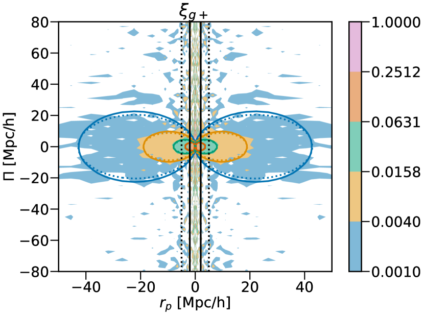
(a)

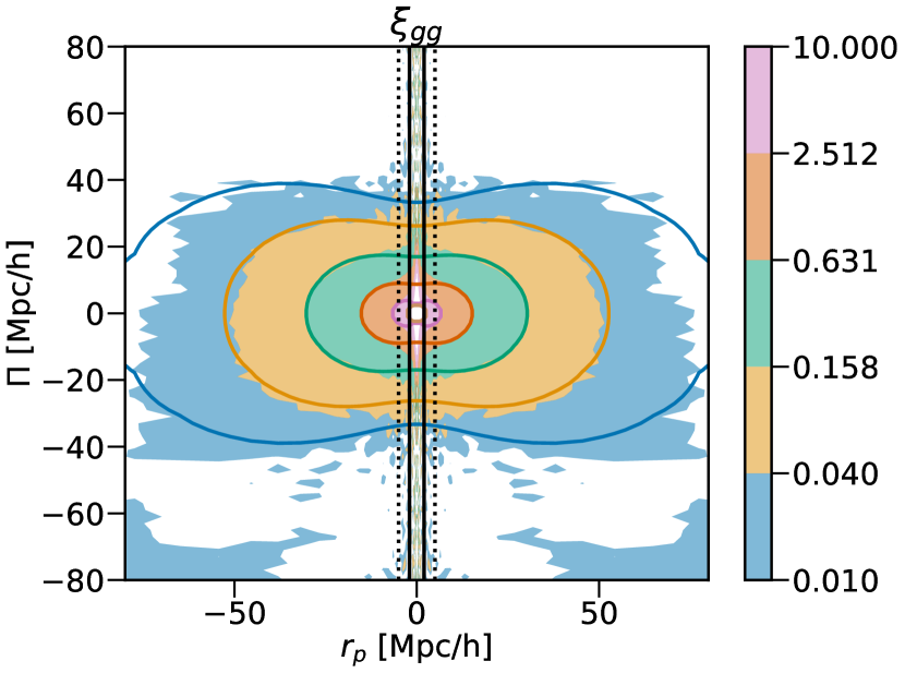
(b)

Figure 1: Galaxy-shape (Fig. 1(a)) and galaxy-galaxy (Fig. 1(b)) correlation function measurements for the full LOWZ galaxy sample in the $(r_{\mathrm{p}},\Pi)$ space. The solid contours show the measurements from the data, the solid lines are the model in redshift space (with the Kaiser correction, which is intended to be valid on large scales), and dotted lines are the model without redshift space correction (shown only for $\xi_{g+}$). We see that the model appears to be consistent with the data on large scales ($r_{\mathrm{p}}\gtrsim 5h^{-1}\text{Mpc})$ within the statistical uncertainties. On scales below a few Mpc$/h$, there are considerable deviations, especially due to the Fingers-of-God effect (FoG), which is not captured in our models. The vertical solid (dotted) black lines are placed at $r_{\mathrm{p}}=2h^{-1}\text{Mpc}$ ($5h^{-1}\text{Mpc}$). The region with $r_{\mathrm{p}}\leq 5h^{-1}\text{Mpc}$ contains almost all of the FoG effect, and hence we use $r_{\mathrm{p}}>5h^{-1}\text{Mpc}$ when defining the wedged multipole moments from the data and model. By convention $r_{\mathrm{p}}$ is defined to be positive, but the plot has been made with mirror images about $r_{\mathrm{p}}=0$.

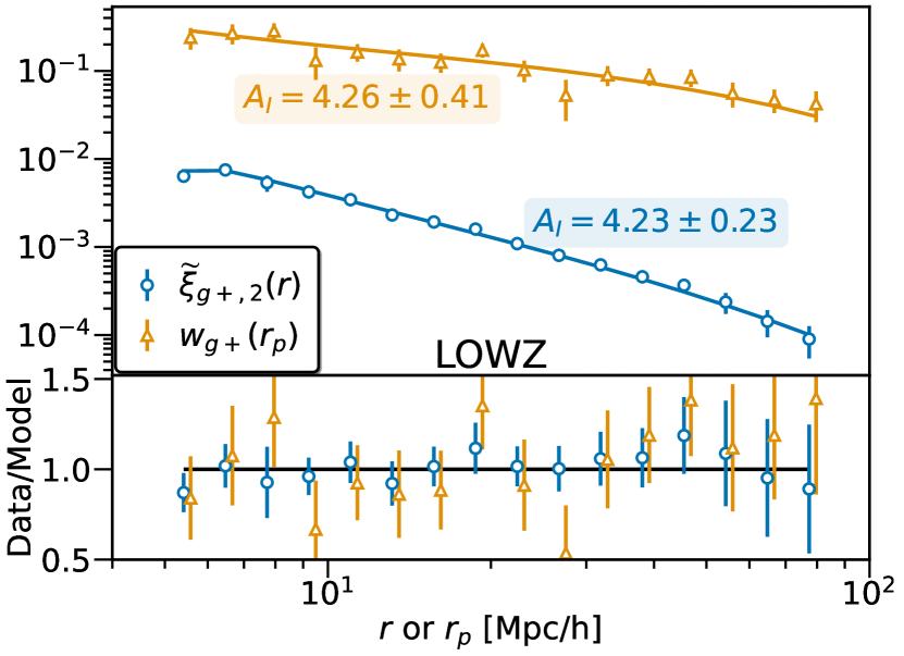
(a)

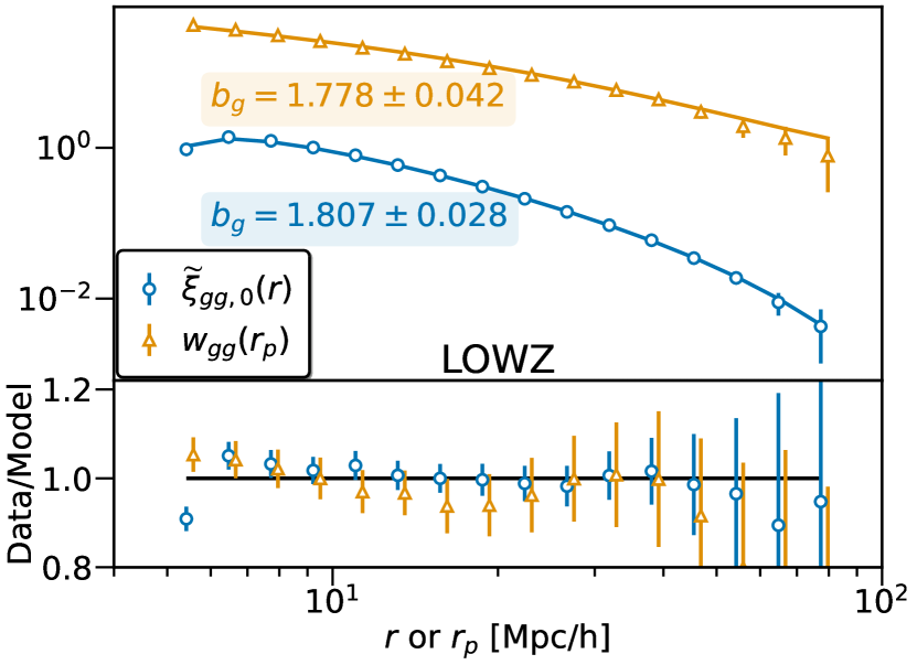
(b)

Figure 2: For the full LOWZ sample, we show $w_{g+}$ and the $\widetilde{\xi}_{g+}$ wedged quadrupole (Fig. 2(a)), and $w_{gg}$ and the $\widetilde{\xi}_{gg}$ wedged monopole (Fig. 2(b)) measurements. The wedged multipoles use a $r_{\mathrm{p}}>5h^{-1}\text{Mpc}$ cut. The solid points show the measurements from data with jackknife errorbars while the solid lines show the model predictions. The lower panel in both figures shows the ratio of data measurements to the model. The model is in excellent agreement with the data on all scales shown, given that we have removed the scales below $r_{\mathrm{p}}=5h^{-1}\text{Mpc}$, as they are affected by non-linearities introduced by the Fingers-of-God effect and non-linear clustering.

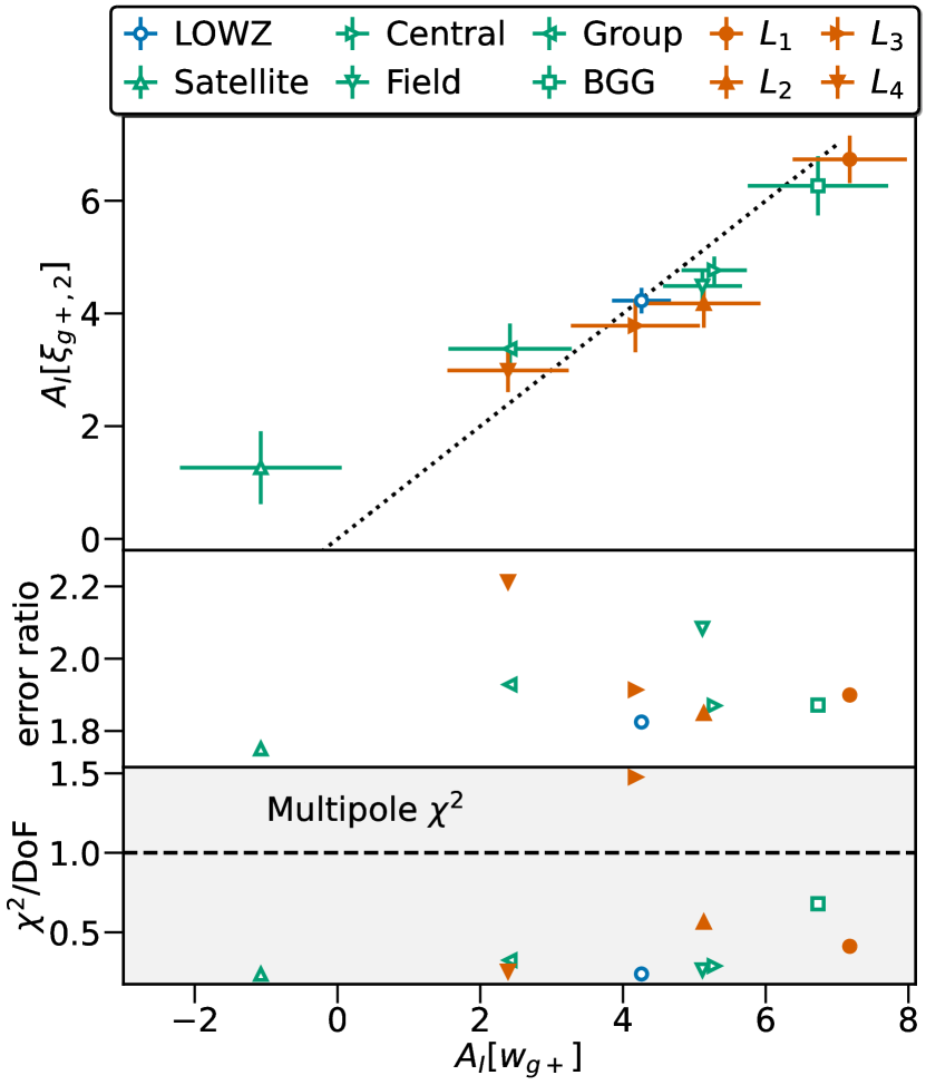
(a)

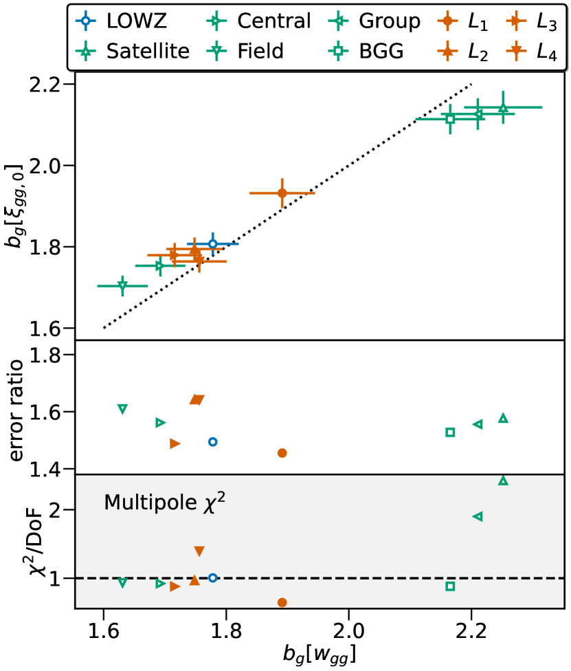
(b)

Figure 3: Upper Panel: Comparison of the model parameters, intrinsic alignment amplitude $A_{I}$ and galaxy bias, $b_{g}$ obtained from fitting the wedged multipole moments of correlation functions (y-axis) and the projected correlation functions (x-axis) for subsamples of the LOWZ sample. The parameters obtained using the two estimators are consistent with each other, indicating that the model is working consistently for both the estimators. Note that the parameters from the two estimators are not expected to match exactly or be tightly correlated since the two estimators are sensitive to different modes in the $(r,\mu)$ or equivalently the $(r_{\mathrm{p}},\Pi$) plane. Middle Panel: The ratio of parameter uncertainties obtained from fits to the wedged multipoles versus those from the projected correlation functions. The multipole moments results in a better signal-to-noise ratio on the parameter estimates, with a factor of $1.5-2$ improvement across all the subsamples. The bottom panel shows the separate $\chi^{2}$ contributions from $\widetilde{\xi}_{g+}$ and $\widetilde{\xi}_{gg}$ for the best fitting parameter values divided by the degrees of freedom (DoF $=16$), which is the number of $r$ or $r_{\mathrm{p}}$ bins fitted minus one (number of model parameters).

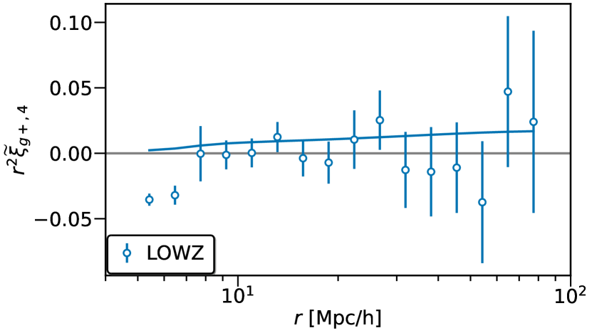
Figure 4: Hexadecapole (wedge) of the galaxy-shape cross-correlation function, $\xi_{g+}$. The open markers with errorbars show the measurements from the full LOWZ sample, while the solid blue line shows the NLA model prediction using the best-fitting parameters from fitting the quadrupole. The hexadecapole measurements are noisy compared to the predicted signal, and since our model also does not include the full non-linear RSD effects, we do not include the hexadecapole when fitting the model to the measurements.

We begin by showing the galaxy clustering and galaxy-shape cross correlation measurements for the full LOWZ sample in the two dimensional space of $(r_{\mathrm{p}},\Pi)$ in Figure 1. The solid contours in the figure show the measurements from the data, while the solid lines show the best-fitting model (to $w_{gg}$ and $w_{g+}$, as discussed later in this section). On large scales, the model is consistent with the data. However, on small scales ($r_{\mathrm{p}}\lesssim 5h^{-1}\text{Mpc}$, marked by vertical dotted lines) there are significant deviations, primarily due to the Fingers-of-God effect. Since the model is not expected to explain the data well on these scales ($r_{\mathrm{p}}\lesssim 5h^{-1}\text{Mpc}$), we exclude these scales when fitting the model and also when computing the wedged multipole moments.

In Figure 2, we show the measurements of both the projected correlation functions ($w_{gg}$, $w_{g+}$) and the lowest order nonzero wedged multipoles (monopole for $\widetilde{\xi}_{gg}$ and quadrupole for $\widetilde{\xi}_{g+}$). When fitting the models, we applied the cuts $r_{\mathrm{p}}>5h^{-1}\text{Mpc}$ for projected correlation functions and $r>5h^{-1}\text{Mpc}$ for wedged multipoles which were computed with $r_{\mathrm{p}}>5h^{-1}\text{Mpc}$ cut. Our simple model with only a linear galaxy bias and IA amplitude as free parameters fits the measurements quite well on these scales. It is important to note that the qualities of these fits does not confirm that the model is complete on those scales, as there are nonzero clustering and IA contributions in higher multipoles, for which the model may struggle to fit $\widetilde{\xi}_{gg}$ down to these scales. Modeling clustering multipoles is a well-explored problem in the literature and we refer the interested reader to publications such as Alam et al. (2017); Vlah & White (2019) and references therein for more information.

Our primary goal in this work is to show that it is possible to extract more information from the IA and clustering multipoles than from the projected estimators commonly used for IA measurements and model constraints. Figure 2 shows this clearly as the multipole moments have a higher signal-to-noise ratio than the projected correlation functions. Furthermore, for the parameters of interest in IA modeling (in this case $A_{I}$), the constraints are improved by almost a factor of $\sim 1.8-2.2$ as shown by the $A_{I}$ values and uncertainties shown on this plot. The quality of the model fits and the parameter values are very similar for both the multipoles and the projected correlation functions, showing that it is better to use the lowest order multipoles instead of projected correlation functions even when the galaxy velocities are not fully modeled.

In Fig. 3, we show the comparison of the IA model parameters obtained by splitting the LOWZ sample into various subsamples as defined in Singh et al. (2017a), encompassing different physical environments and different ranges of intrinsic luminosity. In particular, we divide galaxies based on environment into satellite, central, field, group, and brightest group galaxies (BGGs); and into luminosity bins labeled $L_{1}$–$L_{4}$ based on intrinsic luminosities, with lower numbers corresponding to brighter samples. By doing so, we can check the model quality for subsamples and also whether the improved constraints on IA model parameters persists across these samples.

Both the galaxy bias and IA amplitudes obtained from the two estimators are consistent in value, with the wedged multipoles consistently producing higher signal-to-noise measurements, resulting in factors of $\sim 1.5-1.8$ improvement in the galaxy bias constraints and factors of $\sim 1.8-2$ improvement in $A_{I}$. Since the ability of the model to explain the multipoles at small scales is a concern due to the non-linear effects of redshift space distortions, we show the $\chi^{2}$ of the best-fitting models in the lower panel of Fig. 3. For galaxy clustering, the reduced $\chi^{2}$ is consistent with the expected value of 1, except for the samples dominated by satellite galaxies, namely the ‘group’ sample containing only galaxies within the groups of 2 or more and the ‘satellite’ sample which only selects satellites from the groups. These samples should have the largest effects from non-linear RSD, and hence as expected the model cannot fully describe the data for these samples. For the case of galaxy shape cross correlations, we consistently obtain $\chi^{2}$ values that are $\lesssim 1$, indicating that the model works well and our jackknife covariance may have overestimated the errors somewhat.

In Fig. 4 we show the hexadecapole (wedge) measurements for $\widetilde{\xi}_{g+}$ using the full LOWZ sample. The hexadecapole contribution to $\widetilde{\xi}_{g+}$ arises purely because of the redshift space distortions in the galaxy positions. As shown in Fig. 1(a), these RSD effects are relatively small and hence the hexadecapole signal is expected to be small and noisy. Fig. 4 confirms this expectation, as the measurement is consistent with zero on most scales. We also show the model predictions for comparison and data is consistent with the model on most scales, except for very small scales where our model is not expected to capture the non-linear RSD effects very well. Because of the noise in the measurements and the incompleteness of our model, we do not include the hexadecapole when fitting the model to the measurements.

5.2 Results from the simulation

To gain deeper insight into these results, we also performed the measurements using a state-of-the-art hydrodynamical simulation, the Illustris-TNG (for more details see Section 3). Use of a simulation enables us to explore effects that cannot be separated in the real data, such as the impact of real space vs. redshift space. When fitting the models to the simulated data, we applied the cuts $r_{\mathrm{p}}>2h^{-1}\text{Mpc}$ when computing multipole wedges and also a further cut of $r>4h^{-1}\text{Mpc}$ when fitting the models. Given the smaller size of the simulation box, the lower $r_{\mathrm{p}}$ cut is necessary to obtain sufficient signal to noise in the parameter constraints. Our tests with larger $r_{\mathrm{p}}$ cuts suggest our analysis is not biased (within the noise of the measurements).

In Figure 5, we show the measured multipoles and their fits both in real space and in redshift space. The figure reiterates our findings in observed data: that the parameter constraints are improved when using multipoles while the quality of the fits is also good. The $\chi^{2}$ values per degree of freedom for each of the fits are within 40% of the expected value of 1. For measurements done in real space, the constraints on $A_{I}$ are tighter by a factor 4 than those using projected correlation functions, with reduced $\chi^{2}=0.79$, indicating a well-fit model.

To further investigate the effects of galaxy velocities, we performed the same measurements but in redshift space (row 2 of Fig. 5). The trends for these fits are similar: we get an improvement of almost a factor of 3 in the constraint on $A_{I}$, while the quality of fits is not degraded because of un-modeled non-linear velocity effects. All in all, these results suggest that using multipoles to measure the IA signal improves the constraints on the parameters of interest by a substantial amount, and measurements done in real space and redshift space show consistent results.

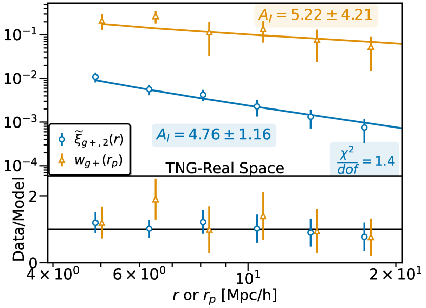
(a)

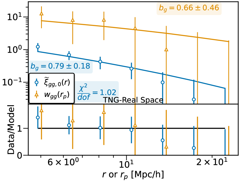
(b)

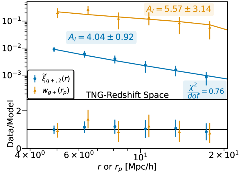
(c)

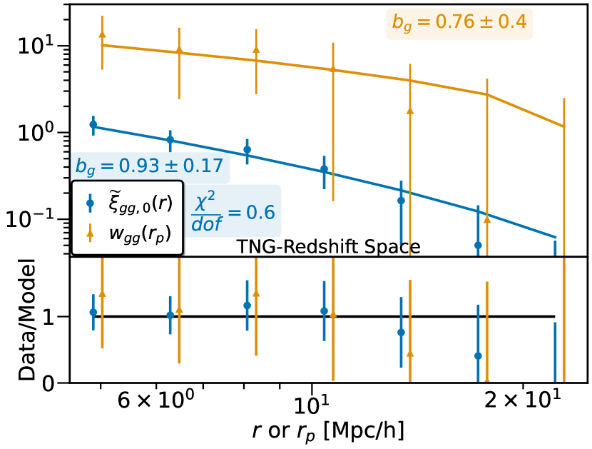
(d)

Figure 5: $\widetilde{\xi}_{g+}$ wedged quadrupole (1st column) and $\widetilde{\xi}_{gg}$ wedged monopole (2nd column) measurements from the elliptical galaxy sample selected in the IllustrisTNG-100 $z=0$ snapshot, along with the corresponding projected correlation functions. Here we show the wedged multipoles with $r_{\mathrm{p}}>2h^{-1}\text{Mpc}$ cuts and we use $r_{\mathrm{min}}>4h^{-1}\text{Mpc}$ for the fits. The first row shows measurements made in real space, whereas the second row is in redshift space. The points show the measurements from the simulation with jackknife errorbars, while the solid lines show the best fitting model. The lower panel in all four figures shows the ratio of the measurements to the model. The model is in good agreement with the data on all scales. There is no significant difference between the real space and the redshift space measurements for the quantities shown here.

6 Conclusions

In this paper, we have demonstrated the performance of a multipole-based estimator for the intrinsic alignment signal, to be employed in direct measurements of alignments using galaxy samples with shapes and spectroscopic redshifts. The goal of using this estimator is to enable a more optimal extraction of information about intrinsic alignment models from the measurements, effectively increasing the statistical constraining power of current and future datasets. In practice, it is only necessary to use the lowest nonzero multipole (i.e., the quadrupole) for the intrinsic alignment signal in order to unlock the benefit of this new estimator.

By applying this estimator to both simulated and real data, we have identified substantial gains in constraining power. For example, when interpreting the measurements using the nonlinear alignment (NLA) model (Bridle & King, 2007), we found a factor of $\sim 2.3$ increase in statistical precision of the alignment amplitude in simulations, and a doubling of the statistical precision in real data. This is equivalent to multiplying the survey area by a factor of 4, given that the constraints are shape noise dominated.

It is worth keeping in mind some potential future improvements in modeling that will be needed to fully exploit the improved constraining power in this multipole-based estimator. First, making use of the improved statistical power in the measurements with multipoles requires that one be able to produce a theoretical prediction in the $(r_{\mathrm{p}},\Pi)$ plane so as to calculate multipoles and produce quantities that can be compared with this estimator. While this is clearly already the case for the NLA model, it may not be as straightforward for other intrinsic alignment methods of interest in the field. However, in most models, the angular dependence is separable from the scale dependence, i.e., the $\mu^{2}$-dependence is separable from the $k$-dependence, and can likely be modeled with a limited number of multipoles in some cases; see, for example, eq. 2.63 in Bakx et al. (2023). Of course, this limitation also exists for projected correlation functions computed with finite line of sight integration length (Baldauf et al., 2010; Singh et al., 2019).

Another potential issue in future is that the increased signal-to-noise in the measurements will necessitate an improved model for interpreting those measurements. Our results suggest that the current model with Halofit and the Kaiser correction is sufficient to model the lowest order multipole wedges (monopole for galaxy auto-correlations and quadrupole for galaxy-shape correlations) using $r_{\mathrm{p}}>5h^{-1}\text{Mpc}$. $r_{\mathrm{p}}\sim 5h^{-1}\text{Mpc}$ is also the scale to which projected correlation functions can be modeled using the same model (Singh et al., 2015). However, this new estimator may require an improved theoretical model with other samples or to push to smaller physical scales.

Finally, while direct IA measurements can be made using high-quality photometric redshifts, additional development would be needed to ascertain how to use a multipole-based estimator in such a case and whether it adds any advantage. The photometric redshift uncertainties modify the expected shape of the signal in the $(r_{p},\Pi)$ plane, smearing out the correlation function along both the $r_{p}$ and $\Pi$ directions, qualitatively similar to RSD effects but with opposite sign and an order of magnitude larger strength (typically, $\Delta z\sim 10^{-3}$ for RSD and $\Delta z\gtrsim 0.01$ for high-quality photometric redshifts). This would require additional modeling and using higher order multipole moments to optimally extract the signal.

In the near future, we anticipate that intrinsic alignment constraints with existing datasets could be productively re-evaluated using this estimator. The resulting improvements in our understanding of intrinsic alignments and their scaling with luminosity, colour, and more (e.g., Samuroff et al., 2022) has great potential to improve the systematics mitigation process for cosmological weak lensing measurements with ongoing and upcoming surveys.

Data Availability Statement

The data and software associated with this work are available on the World Wide Web. The simulation catalog data is available at https://github.com/McWilliamsCenter/gal_decomp_paper, while the SDSS-III BOSS LOWZ catalog is available at https://cosmo.vera.psc.edu/SDSS_shape_catalog/. The software used to calculate the correlation functions in this work is available at https://github.com/sukhdeep2/corr_pc, and the analysis codes will be made available upon reasonable request to the authors.

References

- Abazajian et al. (2009) Abazajian K. N., et al., 2009, ApJS, 182, 543
- Ahn et al. (2012) Ahn C. P., et al., 2012, ApJS, 203, 21
- Aihara et al. (2011) Aihara H., et al., 2011, ApJS, 193, 29
- Akeson et al. (2019) Akeson R., et al., 2019, preprint, (arXiv:1902.05569)
- Alam et al. (2017) Alam S., et al., 2017, MNRAS, 470, 2617
- Amon et al. (2022) Amon A., et al., 2022, Phys.Rev.D, 105, 023514
- Bakx et al. (2023) Bakx T., Kurita T., Chisari N. E., Vlah Z., Schmidt F., 2023, arXiv e-prints, p. arXiv:2303.15565
- Baldauf et al. (2010) Baldauf T., Smith R. E., Seljak U., Mandelbaum R., 2010, Phys.Rev.D, 81, 063531
- Blazek et al. (2015) Blazek J., Vlah Z., Seljak U., 2015, J. Cosmology Astropart. Phys., 2015, 015
- Bolton et al. (2012) Bolton A. S., et al., 2012, AJ, 144, 144
- Bridle & King (2007) Bridle S., King L., 2007, New Journal of Physics, 9, 444
- Catelan et al. (2001) Catelan P., Kamionkowski M., Blandford R. D., 2001, MNRAS, 320, L7
- Dalal et al. (2023) Dalal R., et al., 2023, preprint, (arXiv:2304.00701)
- Davis et al. (1985) Davis M., Efstathiou G., Frenk C. S., White S. D. M., 1985, ApJ, 292, 371
- Dawson et al. (2013) Dawson K. S., et al., 2013, AJ, 145, 10
- Eisenstein et al. (2001) Eisenstein D. J., et al., 2001, AJ, 122, 2267
- Fortuna et al. (2021a) Fortuna M. C., Hoekstra H., Joachimi B., Johnston H., Chisari N. E., Georgiou C., Mahony C., 2021a, MNRAS, 501, 2983
- Fortuna et al. (2021b) Fortuna M. C., et al., 2021b, A&A, 654, A76
- Fukugita et al. (1996) Fukugita M., Ichikawa T., Gunn J. E., Doi M., Shimasaku K., Schneider D. P., 1996, AJ, 111, 1748
- Gunn et al. (1998) Gunn J. E., et al., 1998, AJ, 116, 3040
- Gunn et al. (2006) Gunn J. E., et al., 2006, AJ, 131, 2332
- Hartlap et al. (2007) Hartlap J., Simon P., Schneider P., 2007, A&A, 464, 399
- Hirata & Seljak (2003) Hirata C., Seljak U., 2003, MNRAS, 343, 459
- Hirata et al. (2007) Hirata C. M., Mandelbaum R., Ishak M., Seljak U., Nichol R., Pimbblet K. A., Ross N. P., Wake D., 2007, MNRAS, 381, 1197
- Hogg et al. (2001) Hogg D. W., Finkbeiner D. P., Schlegel D. J., Gunn J. E., 2001, AJ, 122, 2129
- Ivezić et al. (2004) Ivezić Ž., et al., 2004, Astronomische Nachrichten, 325, 583
- Ivezić et al. (2019) Ivezić Ž., et al., 2019, ApJ, 873, 111
- Jagvaral et al. (2022a) Jagvaral Y., Campbell D., Mandelbaum R., Rau M. M., 2022a, MNRAS, 509, 1764
- Jagvaral et al. (2022b) Jagvaral Y., Singh S., Mandelbaum R., 2022b, MNRAS, 514, 1021
- Joachimi et al. (2011) Joachimi B., Mandelbaum R., Abdalla F. B., Bridle S. L., 2011, A&A, 527, A26
- Joachimi et al. (2015) Joachimi B., et al., 2015, Space Sci.Rev., 193, 1
- Johnston et al. (2019) Johnston H., et al., 2019, A&A, 624, A30
- Kaiser (1987) Kaiser N., 1987, MNRAS, 227, 1
- Kazin et al. (2013) Kazin E. A., et al., 2013, MNRAS, 435, 64
- Kilbinger (2015) Kilbinger M., 2015, Reports on Progress in Physics, 78, 086901
- Kurita et al. (2021) Kurita T., Takada M., Nishimichi T., Takahashi R., Osato K., Kobayashi Y., 2021, MNRAS, 501, 833
- Landy & Szalay (1993) Landy S. D., Szalay A. S., 1993, ApJ, 412, 64
- Laureijs et al. (2011) Laureijs R., et al., 2011, preprint, (arXiv:1110.3193)
- Li et al. (2019) Li Y., Singh S., Yu B., Feng Y., Seljak U., 2019, J. Cosmology Astropart. Phys., 2019, 016
- Li et al. (2023) Li X., et al., 2023, preprint, (arXiv:2304.00702)
- Lupton et al. (2001) Lupton R., Gunn J. E., Ivezić Z., Knapp G. R., Kent S., 2001, in Harnden F. R. J., Primini F. A., Payne H. E., eds, Astronomical Society of the Pacific Conference Series Vol. 238, Astronomical Data Analysis Software and Systems X. p. 269 (arXiv:astro-ph/0101420), doi:10.48550/arXiv.astro-ph/0101420
- Mandelbaum et al. (2006) Mandelbaum R., Hirata C. M., Ishak M., Seljak U., Brinkmann J., 2006, MNRAS, 367, 611
- Mandelbaum et al. (2011) Mandelbaum R., et al., 2011, MNRAS, 410, 844
- Mandelbaum et al. (2018) Mandelbaum R., et al., 2018, MNRAS, 481, 3170
- Manera et al. (2015) Manera M., et al., 2015, MNRAS, 447, 437
- Marinacci et al. (2018) Marinacci F., et al., 2018, Mon. Not. Roy. Astron. Soc., 480, 5113
- Naiman et al. (2018) Naiman J. P., et al., 2018, MNRAS, 477, 1206
- Nelson et al. (2018) Nelson D., et al., 2018, Mon. Not. Roy. Astron. Soc., 475, 624
- Nelson et al. (2019) Nelson D., et al., 2019, Computational Astrophysics and Cosmology, 6, 2
- Okumura et al. (2009) Okumura T., Jing Y. P., Li C., 2009, ApJ, 694, 214
- Okumura et al. (2020) Okumura T., Taruya A., Nishimichi T., 2020, MNRAS, 494, 694
- Padmanabhan et al. (2008) Padmanabhan N., et al., 2008, ApJ, 674, 1217
- Pier et al. (2003) Pier J. R., Munn J. A., Hindsley R. B., Hennessy G. S., Kent S. M., Lupton R. H., Ivezić Ž., 2003, AJ, 125, 1559
- Pillepich et al. (2018a) Pillepich A., et al., 2018a, MNRAS, 473, 4077
- Pillepich et al. (2018b) Pillepich A., et al., 2018b, MNRAS, 475, 648
- Planck Collaboration et al. (2016) Planck Collaboration et al., 2016, A&A, 594, A13
- Reid et al. (2016) Reid B., et al., 2016, MNRAS, 455, 1553
- Reyes et al. (2012) Reyes R., Mandelbaum R., Gunn J. E., Nakajima R., Seljak U., Hirata C. M., 2012, MNRAS, 425, 2610
- Richards et al. (2002) Richards G. T., et al., 2002, AJ, 123, 2945
- Samuroff et al. (2022) Samuroff S., et al., 2022, preprint, (arXiv:2212.11319)
- Sánchez et al. (2017) Sánchez A. G., et al., 2017, MNRAS, 464, 1640
- Secco et al. (2022) Secco L. F., et al., 2022, Phys.Rev.D, 105, 023515
- Singh & Mandelbaum (2016) Singh S., Mandelbaum R., 2016, MNRAS, 457, 2301
- Singh et al. (2015) Singh S., Mandelbaum R., More S., 2015, MNRAS, 450, 2195
- Singh et al. (2017a) Singh S., Mandelbaum R., Brownstein J. R., 2017a, MNRAS, 464, 2120
- Singh et al. (2017b) Singh S., Mandelbaum R., Seljak U., Slosar A., Vazquez Gonzalez J., 2017b, MNRAS, 471, 3827
- Singh et al. (2019) Singh S., Alam S., Mandelbaum R., Seljak U., Rodriguez-Torres S., Ho S., 2019, MNRAS, 482, 785
- Singh et al. (2021) Singh S., Yu B., Seljak U., 2021, MNRAS, 501, 4167
- Smee et al. (2013) Smee S. A., et al., 2013, AJ, 146, 32
- Smith et al. (2002) Smith J. A., et al., 2002, AJ, 123, 2121
- Smith et al. (2003) Smith R. E., et al., 2003, MNRAS, 341, 1311
- Springel (2010) Springel V., 2010, MNRAS, 401, 791
- Springel et al. (2001) Springel V., White S. D. M., Tormen G., Kauffmann G., 2001, MNRAS, 328, 726
- Springel et al. (2018) Springel V., et al., 2018, Mon. Not. Roy. Astron. Soc., 475, 676
- Strauss et al. (2002) Strauss M. A., et al., 2002, AJ, 124, 1810
- Takahashi et al. (2012) Takahashi R., Sato M., Nishimichi T., Taruya A., Oguri M., 2012, ApJ, 761, 152
- Troxel & Ishak (2015) Troxel M. A., Ishak M., 2015, Phys.Rep., 558, 1
- Tucker et al. (2006) Tucker D. L., et al., 2006, Astronomische Nachrichten, 327, 821
- Vlah & White (2019) Vlah Z., White M., 2019, J. Cosmology Astropart. Phys., 2019, 007
- Vlah et al. (2020) Vlah Z., Chisari N. E., Schmidt F., 2020, J. Cosmology Astropart. Phys., 2020, 025
- Weinberg et al. (2013) Weinberg D. H., Mortonson M. J., Eisenstein D. J., Hirata C., Riess A. G., Rozo E., 2013, Phys.Rep., 530, 87
- Weinberger et al. (2017) Weinberger R., et al., 2017, MNRAS, 465, 3291
- Yao et al. (2019) Yao J., Ishak M., Troxel M. A., LSST Dark Energy Science Collaboration 2019, MNRAS, 483, 276
- York et al. (2000) York D. G., et al., 2000, AJ, 120, 1579
- van den Busch et al. (2022) van den Busch J. L., et al., 2022, A&A, 664, A170