\stackMath\tikzfeynmanset

fermion1/.style= /tikz/postaction= /tikz/decoration= markings, mark=at position 0.6 with \arrow[scale=1.2,>=stealth]>; , , /tikz/decorate=true, , , aainstitutetext: Helmholtz-Institut fรผr Strahlen- und Kernphysik (Theorie) and
Bethe Center for Theoretical Physics, Universitรคt Bonn, 53115 Bonn, Germany
bbinstitutetext: Institut fรผr Kernphysik (Theorie), Institute for Advanced Simulation, and
Jรผlich Center for Hadron Physics, Forschungszentrum Jรผlich, 52425 Jรผlich, Germany

Correlations of $C$ and $CP$ violation in $\eta\to\pi^{0}\ell^{+}\ell^{-}$ and $\eta^{\prime}\to\eta\ell^{+}\ell^{-}$

Hakan Akdag a โ€ƒโ€ƒ Bastian Kubis b โ€ƒโ€ƒ and Andreas Wirzba akdag@hiskp.uni-bonn.de kubis@hiskp.uni-bonn.de a.wirzba@fz-juelich.de
Abstract

Based on recent progress in the systematic analysis of $C$ and $CP$ violation in the light-meson sector, we calculate the $C$-odd transition amplitudes $\eta\to\pi^{0}\ell^{+}\ell^{-}$ and $\eta^{\prime}\to\eta\ell^{+}\ell^{-}$. Focusing on long-distance contributions driven by the lowest-lying hadronic intermediate states, we work out the correlations between these beyond-the-Standard-Model signals and the Dalitz-plot asymmetries in $\eta\rightarrow\pi^{0}\pi^{+}\pi^{-}$ and $\eta^{\prime}\rightarrow\eta\pi^{+}\pi^{-}$, using dispersion theory.

1 Introduction

In the recent past new light was shed on analyzing patterns of $C$- and $CP$-odd signals in hadronic decays concerning the $\eta$-sector. First, Ref.ย Gardner:2019nid provided a new theoretical framework for $C$ย violation in $\eta\to\pi^{0}\pi^{+}\pi^{-}$, which was neglected since the 1960s and allows one to decompose the decay amplitude into contributions of different isospin transitions, hence to disentangle the underlying beyond-the-Standard-Model (BSM) operators of isospin $I=0$ and $I=2$. This analysis has been improved and extended to $\eta^{\prime}\to\pi^{0}\pi^{+}\pi^{-}$ as well as $\eta^{\prime}\to\eta\pi^{+}\pi^{-}$ in Ref.ย Akdag:2021efj , which relied on the dispersion-theoretical Khuriโ€“Treiman framework. Motivated by these analyses, Ref.ย Akdag:2022sbn derived the full set of $C$- and $CP$-violating quark-level operators for flavor-conserving, lepton- and baryon-number-preserving transitions in the low-energy effective field theory (LEFT) and matched them onto a $T$-odd and $P$-even (ToPe) analog of chiral perturbation theory (ToPe$\chi$PT) (cf.ย also Refs.ย Shi:2017ffh ; Gardner:prep ). The latter allows us to access all corresponding $C$- and $CP$-odd mesonic interactions.

One may use the formalisms addressed in the previous paragraph to investigate the correlation of $T$-odd and $P$-even forces between different decays. In this sense we consider $C$- and $CP$-violating radiative decays of $\eta$ and $\eta^{\prime}$. In the following, we denote both mesons with $\eta^{(\prime)}$. Given that $\eta^{(\prime)}$ as well as $\pi^{0}$ have the eigenvalue $C=+1$ but photons have $C=-1$, $C$ is violated in general if $\eta^{(\prime)}$ decays into an arbitrary number of uncharged pions and an odd number of photons. This consideration also holds for radiative decays of the $\eta^{\prime}$ into an $\eta$. In the following we will focus on the radiative $C$-odd decays $\eta\to\pi^{0}\gamma^{(\ast)}$ and $\eta^{\prime}\to\eta\gamma^{(\ast)}$. To shorten the notation we will refer to both processes collectively by $X\to Y\gamma^{(\ast)}$. Angular momentum conservation demands the final state to be in a relative $P$-wave. Consequently, parity is conserved and the decays at hand additionally violate $CP$, thus offering an opportunity to investigate ToPe forces. The decay into a real, transverse photon violates both gauge invariance and the conservation of angular momentumย Sakurai:1964 ; Gan:2020aco . Therefore, the focus shall be laid on $X\rightarrow Y\gamma^{\ast}\to Y\ell^{+}\ell^{-}$, where the off-shell photon decays subsequently into a pair of charged leptons. At the theoretical front, the investigation of this BSM one-photon exchange urgently requires an updateย Bernstein:1965hj ; Barrett:1965ia in comparison to analyses of the SM contribution, cf.ย Refs.ย LlewellynSmith:1967 ; Cheng:1967zza ; Smith:1968 ; Ng:1992 ; Ng:1993 ; Escribano:2020rfs ; Schaefer:2023 , as well as studies of other BSM effects in these decaysย Gan:2020aco ; Escribano:2022zgm . From an experimental point of view, bounds on all the leptonic channels have already been setย Dzhelyadin:1980ti ; CLEO:1999nsy ; WASA-at-COSY:2018jdv and may become more stringent in future measurementsย Gan:2009zzd ; JEF:2014 ; Gan:2015nyc ; JEF:2017 ; Gatto:2016rae ; Gatto:2019dhj ; REDTOP:2022slw .

Assuming that the underlying new physics generating the $C$- and $CP$-odd decays $X\to Y\ell^{+}\ell^{-}$ originates from sources at some high-energy scale $\Lambda$, there are in principle three dominant mechanisms to consider:

  1. 1.

    short-distance contributions to the dilepton final state,

  2. 2.

    long-distance contributions caused by $C$- and $CP$-odd photonโ€“hadron couplings,

  3. 3.

    long-distance contributions induced by hadronic intermediate states.

For the first two classes we rely on ToPe$\chi$PT as proposed in Ref.ย Akdag:2022sbn . One intricacy of the contribution by hadronic intermediate states is that the subsequent photon is allowed to have both isoscalar and isovector components. To predict the involved isovector transitions in a model-independent way, one can utilize the $X\to Y\pi^{+}\pi^{-}$ amplitudes derived non-perturbatively in the Khuriโ€“Treiman frameworkย Akdag:2021efj and establish dispersion relations for the respective transition form factors. Analogous relations have previously been derived for the decays $\omega,\,\phi,\,J/\psi\to\pi^{0}\gamma^{\ast}$ย Koepp:1974da ; Schneider:2012ez ; Danilkin:2014cra ; Kubis:2014gka ; JPAC:2020umo , which are compatible with conservation of all discrete symmetries. In addition, we sketch an idea of how to evaluate the isoscalar contribution of the photon, employing a less sophisticated, but still symmetry-driven, vector-meson-dominance (VMD) model for the decay $X\to Y\gamma^{*}$. By an analytic continuation of the three-body amplitudes $X\to Y\pi^{+}\pi^{-}$ to the second Riemann sheet we can extract $\rho YX$ couplings, which can be related to the relevant ones with the same total isospin in the VMD model using $SU(3)$ symmetry and naive dimensional analysis (NDA).

To extract observables of the $C$- and $CP$-violating contribution in $X\to Y\ell^{+}\ell^{-}$ driven by a one-photon exchange we pursue the following strategy. First, we consider the phenomenology behind the three mechanisms mentioned above in Sect.ย 2. For this purpose we lay out the basic definitions of kinematics and relate the amplitude to the (differential) decay widths in Sect.ย 2.1. We discuss the short-range semi-leptonic operators, the long-range direct photonโ€“hadron couplings, and the long-range hadronic contributions on a general level in Sects.ย 2.2โ€“2.4, respectively. Subsequently, Sect.ย 2.5 includes a discussion of the feasibility of these contributions. The remainder of the article solely focuses on long-distance contributions with hadronic intermediate states. In Sect.ย 3 we investigate the isovector contributions to these hadronic long-range effects. For this purpose, we first sketch the $C$- and $CP$-odd contributions to the decays $X\to Y\pi^{+}\pi^{-}$ in Sect.ย 3.1, which serve as input to the respective transition form factors. The computation of the latter is discussed in Sect.ย 3.2. In Sect.ย 3.3, we extract the corresponding $C$-odd couplings of the $\rho(770)$ resonance to $\eta\pi^{0}$ and $\eta^{\prime}\eta$ by analytic continuation in the complex-energy plane. Subsequently, we estimate the size of the hadronic long-range effects in the isoscalar parts in Sect.ย 4. Finally, we present the predicted upper limits on the branching ratios in Sect.ย 5 and close with a short summary and outlook in Sect.ย 6.

2 Phenomenology

{feynman}{feynhand}\vertex\vertex\vertex$X$\vertex\vertex\vertex$Y$\vertex$\ell^{+}$\vertex$\ell^{-}$\vertex\vertexย ย ย \feynmandiagram{feynman}{feynhand}\vertex\vertex\vertex$X$\vertex\vertex\vertex\vertex$\ell^{+}$\vertex$\ell^{-}$\vertex\vertex$Y$\feynmandiagram$\gamma^{\ast}${feynman}{feynhand}\vertex\vertex\vertex$X$\vertexย ย ย ย \vertexย ย ย ย \vertex\vertex\vertex$\ell^{+}$\vertex$\ell^{-}$\vertex\vertex$Y$\feynmandiagram$\pi^{+}$ $\pi^{-}$ $\gamma^{\ast}${feynman}{feynhand}\vertex\vertex\vertex$X$\vertex\vertex\vertex\vertex\vertex$\ell^{+}$\vertex$\ell^{-}$\vertex\vertex$Y$\feynmandiagram$\ V$ $\gamma^{\ast}$

Figure 1: Contributions to the $C$- and $CP$-odd decay $X\to Y\ell^{+}\ell^{-}$. The first diagram describes a short-range semi-leptonic four-point vertex, the second one includes a long-range hadronโ€“photon coupling, while the last two diagrams account for possible hadronic intermediate states. Among the latter, the pion loop corresponds to an isovector transition while the vector-meson conversion respects the isoscalar part of the virtual photon. The black dot, the red box, the gray circle, and the blue box refer to different $C$- and $CP$-violating vertices, while the white circle is $C$- and $CP$-conserving.

In this section we discuss the phenomenological importance of the three mechanisms driving $X\to Y\ell^{+}\ell^{-}$ and provide the model-independent expressions for them. As an illustration we depict the different contributions in Fig.ย 1. For simplicity we adapt the notation and conventions introduced for the construction of operators in ToPe$\chi$PT in Ref.ย Akdag:2022sbn without further details.

2.1 Kinematics

Consider the transition amplitude $X(P)\to Y(p)\ell^{+}(p_{\ell^{+}})\ell^{-}(p_{\ell^{-}})$, with two pseudoscalars $X$ and $Y$ of masses $M_{X}>M_{Y}$. Conventionally, we describe the three-body decay in terms of the Lorentz invariants

s=(Pโˆ’p)2,tโ„“=(Pโˆ’pโ„“+)2,uโ„“=(Pโˆ’pโ„“โˆ’)2.formulae-sequence๐‘ superscript๐‘ƒ๐‘2formulae-sequencesubscript๐‘กโ„“superscript๐‘ƒsubscript๐‘superscriptโ„“2subscript๐‘ขโ„“superscript๐‘ƒsubscript๐‘superscriptโ„“2s=(P-p)^{2},\qquad t_{\ell}=(P-p_{\ell^{+}})^{2},\qquad u_{\ell}=(P-p_{\ell^{-}})^{2}. (1)

With the electromagnetic quark current

$$J_{\mu}=\sum_{f}Q_{f}\bar{q}_{f}\gamma_{\mu}q_{f}\,,$$ (2)

where $Q_{f}$ indicates the electric charge of the respective quarks with flavor $f$ and is conventionally used in units of the proton charge $e$, the singularity-free electromagnetic transition form factor FXโ€‹Yโ€‹(s)subscript๐น๐‘‹๐‘Œ๐‘ F_{XY}(s) in $X\to Y\gamma^{*}$ can be decomposed by Poincarรฉ invariance and current conservation asย Bernstein:1965hj ; DAmbrosio:1998gur

โŸจYโ€‹(p)|Jฮผโ€‹(0)|Xโ€‹(P)โŸฉ=โˆ’iโ€‹[sโ€‹(P+p)ฮผโˆ’(P2โˆ’p2)โ€‹qฮผ]โ€‹FXโ€‹Yโ€‹(s)โ‰กโˆ’iโ€‹Qฮผโ€‹FXโ€‹Yโ€‹(s).quantum-operator-product๐‘Œ๐‘subscript๐ฝ๐œ‡0๐‘‹๐‘ƒ๐‘–delimited-[]๐‘ subscript๐‘ƒ๐‘๐œ‡superscript๐‘ƒ2superscript๐‘2subscript๐‘ž๐œ‡subscript๐น๐‘‹๐‘Œ๐‘ ๐‘–subscript๐‘„๐œ‡subscript๐น๐‘‹๐‘Œ๐‘ \langle Y(p)|J_{\mu}(0)|X(P)\rangle=-i\left[s(P+p)_{\mu}-(P^{2}-p^{2})q_{\mu}\right]\,F_{XY}(s)\equiv-iQ_{\mu}\,F_{XY}(s)\,. (3)

Here we introduced the photonโ€™s momentum $q_{\mu}=(P-p)_{\mu}$. Note that FXโ€‹Yโ€‹(s)subscript๐น๐‘‹๐‘Œ๐‘ F_{XY}(s) thus defined is real at leading order in ToPe$\chi$PT. Upon contraction with the lepton current the full decay amplitude becomes

iโ€‹โ„ณโ€‹(Xโ†’Yโ€‹โ„“+โ€‹โ„“โˆ’)=e2โ€‹(P+p)ฮผโ€‹FXโ€‹Yโ€‹(s)โ€‹uยฏrโ€‹(pโ„“โˆ’)โ€‹ฮณฮผโ€‹vrโ€ฒโ€‹(pโ„“+),๐‘–โ„ณโ†’๐‘‹๐‘Œsuperscriptโ„“superscriptโ„“superscript๐‘’2subscript๐‘ƒ๐‘๐œ‡subscript๐น๐‘‹๐‘Œ๐‘ subscriptยฏ๐‘ข๐‘Ÿsubscript๐‘superscriptโ„“superscript๐›พ๐œ‡subscript๐‘ฃsuperscript๐‘Ÿโ€ฒsubscript๐‘superscriptโ„“i\mathcal{M}(X\to Y\ell^{+}\ell^{-})=e^{2}\,(P+p)_{\mu}F_{XY}(s)\,\bar{u}_{r}(p_{\ell^{-}})\gamma^{\mu}v_{r^{\prime}}(p_{\ell^{+}}), (4)

where the term proportional to $q_{\mu}$ drops out due to current conservationย Bernstein:1965hj . In the course of this work, we will see explicitly that the amplitude of each mechanism restores this functional form. Taking the squared absolute value and summing over the lepton spins, one may obtain the doubly differential decay widthย Kubis:2010mp

dโ€‹ฮ“โ€‹(Xโ†’Yโ€‹โ„“+โ€‹โ„“โˆ’)dโ€‹sโ€‹dโ€‹ฯ„=ฮฑ216โ€‹ฯ€โ€‹MX3โ€‹(ฮปโ€‹(s,MX2,MY2)โˆ’ฯ„2)โ€‹|FXโ€‹Yโ€‹(s)|2,dฮ“โ†’๐‘‹๐‘Œsuperscriptโ„“superscriptโ„“d๐‘ d๐œsuperscript๐›ผ216๐œ‹superscriptsubscript๐‘€๐‘‹3๐œ†๐‘ superscriptsubscript๐‘€๐‘‹2superscriptsubscript๐‘€๐‘Œ2superscript๐œ2superscriptsubscript๐น๐‘‹๐‘Œ๐‘ 2\frac{\text{d}\Gamma(X\to Y\ell^{+}\ell^{-})}{\text{d}s\,\text{d}\tau}=\frac{\alpha^{2}}{16\pi M_{X}^{3}}\,\left(\lambda\big{(}s,M_{X}^{2},M_{Y}^{2}\big{)}-\tau^{2}\right)\,|F_{XY}(s)|^{2}, (5)

in terms of the electromagnetic fine-structure constant $\alpha=e^{2}/4\pi$, the Kรคllรฉn function $\lambda(x,y,z)=x^{2}+y^{2}+z^{2}-2(xy+xz+yz)$, and the Lorentz invariant $\tau=t_{\ell}-u_{\ell}$. The $\tau$-integration can be carried out analytically, giving

dโ€‹ฮ“โ€‹(Xโ†’Yโ€‹โ„“+โ€‹โ„“โˆ’)dโ€‹s=ฮฑ28โ€‹ฯ€โ€‹MX3โ€‹ฮป3/2โ€‹(s,MX2,MY2)โ€‹ฯƒโ„“โ€‹(s)โ€‹(1โˆ’ฯƒโ„“2โ€‹(s)3)โ€‹|FXโ€‹Yโ€‹(s)|2,dฮ“โ†’๐‘‹๐‘Œsuperscriptโ„“superscriptโ„“d๐‘ superscript๐›ผ28๐œ‹superscriptsubscript๐‘€๐‘‹3superscript๐œ†32๐‘ superscriptsubscript๐‘€๐‘‹2superscriptsubscript๐‘€๐‘Œ2subscript๐œŽโ„“๐‘ 1subscriptsuperscript๐œŽ2โ„“๐‘ 3superscriptsubscript๐น๐‘‹๐‘Œ๐‘ 2\frac{\text{d}\Gamma(X\to Y\ell^{+}\ell^{-})}{\text{d}s}=\frac{\alpha^{2}}{8\pi M_{X}^{3}}\,\lambda^{3/2}\big{(}s,M_{X}^{2},M_{Y}^{2}\big{)}\,\sigma_{\ell}(s)\left(1-\frac{\sigma^{2}_{\ell}(s)}{3}\right)\,|F_{XY}(s)|^{2}, (6)

where ฯƒโ„“โ€‹(s)=1โˆ’4โ€‹mโ„“2/ssubscript๐œŽโ„“๐‘ 14superscriptsubscript๐‘šโ„“2๐‘ \sigma_{\ell}(s)=\sqrt{1-4m_{\ell}^{2}/s} and the physical range is restricted to sโˆˆ(4โ€‹mโ„“2,(MXโˆ’MY)2)๐‘ 4superscriptsubscript๐‘šโ„“2superscriptsubscript๐‘€๐‘‹subscript๐‘€๐‘Œ2s\in\left(4m_{\ell}^{2},(M_{X}-M_{Y})^{2}\right). Throughout, we use the masses $m_{e}=0.51\,\text{MeV}$, $m_{\mu}=105.66\,\text{MeV}$, $M_{\eta}=547.86\,\text{MeV}$, $M_{\eta^{\prime}}=957.78\,\text{MeV}$, $M_{\pi^{\pm}}=139.57\,\text{MeV}$, and $M_{\pi^{0}}=134.98\,\text{MeV}$ย Workman:2022ynf . For later use, we also quote the vector-meson masses $M_{\rho}=775\,\text{MeV}$ and $M_{\omega}=782.66\,\text{MeV}$ย Workman:2022ynf . The errors and additional decimal digits on all of these masses are negligible in our analysis.

2.2 Direct semi-leptonic contributions to $X\to Y\ell^{+}\ell^{-}$

In Ref.ย Akdag:2022sbn it was shown that the only $C$-odd, $P$-even semi-leptonic four-point vertex to $\eta\to\pi^{0}\ell^{+}\ell^{-}$ at lowest order in the QED fine-structure constant and soft momenta originates from the dimension-8 LEFT operator

$$\mathcal{O}_{\ell\psi}^{(u)}\equiv\frac{c_{\ell\psi}^{(u)}}{\Lambda^{4}}\,\bar{\ell}\gamma^{\mu}\ell\bar{\psi}\gamma^{\nu}T^{a}\psi G^{a}_{\mu\nu}\,,$$ (7)

where $c_{\ell\psi}^{(u)}$ denotes flavor-dependent Wilson coefficients.111In contrast, $CP$-violating quarkโ€“lepton operators that contribute to these decays but are $C$-even and $P$-odd already appear at dimension 6ย Sanchez-Puertas:2018tnp ; Escribano:2022zgm . The choice of the high-energy scale $\Lambda$ depends on the interpretation of the ToPe operators: in the picture of LEFT, $\Lambda$ can be in the order of the electroweak scale, while in the spirit of the Standard Model effective field theory $\Lambda$ is a typical BSM scale. The respective leading ToPe$\chi$PT operators in the large-$N_{c}$ limit readย Akdag:2022sbn

$\displaystyle\bar{X}_{\ell\psi}^{(u)}\supset\frac{c^{(u)}_{\ell\psi}}{\Lambda^{4}}\,\bar{g}_{1}^{(u)}\,i\varphi$ โŸจฮปLโ€‹โˆ‚ฮผUยฏโ€ โ€‹Uยฏโˆ’ฮปRโ€‹โˆ‚ฮผUยฏโ€‹Uยฏโ€ โŸฉโ€‹โ„“ยฏโ€‹ฮณฮผโ€‹โ„“,delimited-โŸจโŸฉsubscript๐œ†๐ฟsubscript๐œ‡superscriptยฏ๐‘ˆโ€ ยฏ๐‘ˆsubscript๐œ†๐‘…subscript๐œ‡ยฏ๐‘ˆsuperscriptยฏ๐‘ˆโ€ ยฏโ„“superscript๐›พ๐œ‡โ„“\displaystyle\big{\langle}\lambda_{L}\partial_{\mu}\bar{U}^{\dagger}\bar{U}-\lambda_{R}\partial_{\mu}\bar{U}\bar{U}^{\dagger}\big{\rangle}\bar{\ell}\gamma^{\mu}\ell\,, (8)
\@afterheading

where we employ the simple single-angle $\eta$-$\eta^{\prime}$ mixing schemeย Feldmann:1999uf , for which the singlet component corresponds to

$$\varphi=\frac{\sqrt{2}}{3\sqrt{3}F_{0}}\,\eta+\frac{4}{3\sqrt{3}F_{0}}\,\eta^{\prime}\,.$$ (9)

The meson matrix in the large-$N_{c}$ limit is then given by

$$\bar{U}=\exp\left(\frac{i\bar{\Phi}}{F_{0}}\right)\,,\quad\mathrm{where}\quad\bar{\Phi}=\begin{pmatrix}\frac{1}{\sqrt{3}}\eta^{\prime}+\sqrt{\frac{2}{3}}\eta+\pi^{0}&\sqrt{2}\pi^{+}&\sqrt{2}K^{+}\\ \sqrt{2}\pi^{-}&\frac{1}{\sqrt{3}}\eta^{\prime}+\sqrt{\frac{2}{3}}\eta-\pi^{0}&\sqrt{2}K^{0}\\ \sqrt{2}K^{-}&\sqrt{2}\bar{K}^{0}&\frac{2}{\sqrt{3}}\eta^{\prime}-\sqrt{\frac{2}{3}}\eta\end{pmatrix}\,.$$ (10)

Furthermore, in relationย (8) we have introduced the spurion matrices $\lambda_{L,R}$ in flavor space, which were defined in Ref.ย Akdag:2022sbn and acquire the same physical values, namely $\lambda_{L,R}\in\{\text{diag}(1,0,0),\,\text{diag}(0,1,0),\,\text{diag}(0,0,1)\}$ for the quark flavor ฯˆ=u,d,s๐œ“๐‘ข๐‘‘๐‘ \psi=u,d,s, respectively. Besides, $F_{0}$ denotes the common meson decay constant in the combined chiral and large-$N_{c}$ limit, $F_{0}\lesssim F_{\pi}\approx 92.3\,\text{MeV}$. Summing over $\psi$ and only picking the interactions relevant for our interests, the operator ${\bar{X}}_{\ell\psi}^{(u)}$ gives rise to the leading-order Lagrangians

$\displaystyle\mathcal{L}_{XY\ell^{+}\ell^{-}}=\frac{1}{\Lambda^{4}F_{0}^{2}}\,\mathcal{N}_{X\to Y\ell^{+}\ell^{-}}\bar{\ell}\gamma^{\mu}\ell X\partial_{\mu}Y$ (11)
\@afterheading

with the normalizations

๐’ฉฮทโ†’ฯ€0โ€‹โ„“+โ€‹โ„“โˆ’โ‰ก2โ€‹23โ€‹3โ€‹gยฏ1(u)โ€‹(cโ„“โ€‹u(u)โˆ’cโ„“โ€‹d(u)),๐’ฉฮทโ€ฒโ†’ฮทโ€‹โ„“+โ€‹โ„“โˆ’โ‰ก2โ€‹23โ€‹gยฏ1(u)โ€‹(cโ„“โ€‹u(u)+cโ„“โ€‹d(u)โˆ’2โ€‹cโ„“โ€‹s(u)).formulae-sequencesubscript๐’ฉโ†’๐œ‚superscript๐œ‹0superscriptโ„“superscriptโ„“2233superscriptsubscriptยฏ๐‘”1๐‘ขsuperscriptsubscript๐‘โ„“๐‘ข๐‘ขsuperscriptsubscript๐‘โ„“๐‘‘๐‘ขsubscript๐’ฉโ†’superscript๐œ‚โ€ฒ๐œ‚superscriptโ„“superscriptโ„“223superscriptsubscriptยฏ๐‘”1๐‘ขsuperscriptsubscript๐‘โ„“๐‘ข๐‘ขsuperscriptsubscript๐‘โ„“๐‘‘๐‘ข2superscriptsubscript๐‘โ„“๐‘ ๐‘ข\mathcal{N}_{\eta\to\pi^{0}\ell^{+}\ell^{-}}\equiv\frac{2\sqrt{2}}{3\sqrt{3}}\,\bar{g}_{1}^{(u)}\big{(}c_{\ell u}^{(u)}-c_{\ell d}^{(u)}\big{)}\,,\qquad\mathcal{N}_{\eta^{\prime}\to\eta\ell^{+}\ell^{-}}\equiv\frac{2\sqrt{2}}{3}\,\bar{g}_{1}^{(u)}\big{(}c_{\ell u}^{(u)}+c_{\ell d}^{(u)}-2c_{\ell s}^{(u)}\big{)}\,. (12)

Both processes are uncorrelated as their normalizations are linearly independent; the flavor combinations reflect the isospin and $SU(3)$ structure of the transitions. Making use of the Dirac equation for the leptons, the corresponding matrix element yields

iโ€‹โ„ณ=e2โ€‹(P+p)ฮผโ€‹F1โ€‹(s)โ€‹uยฏrโ€‹(pโ„“โˆ’)โ€‹ฮณฮผโ€‹vrโ€ฒโ€‹(pโ„“+),๐‘–โ„ณsuperscript๐‘’2subscript๐‘ƒ๐‘๐œ‡subscript๐น1๐‘ subscriptยฏ๐‘ข๐‘Ÿsubscript๐‘superscriptโ„“superscript๐›พ๐œ‡subscript๐‘ฃsuperscript๐‘Ÿโ€ฒsubscript๐‘superscriptโ„“i\mathcal{M}=e^{2}(P+p)_{\mu}F_{1}(s)\,\bar{u}_{r}(p_{\ell^{-}})\gamma^{\mu}v_{r^{\prime}}(p_{\ell^{+}})\,, (13)

with

F1โ€‹(s)โ‰กโˆ’12โ€‹e2โ€‹ฮ›4โ€‹F02โ€‹๐’ฉXโ†’Yโ€‹โ„“+โ€‹โ„“โˆ’โˆผโˆ’1ฮ›4โ€‹2โ€‹ฯ€โ€‹F02e2=โˆ’F022โ€‹ฮฑโ€‹ฮ›4.subscript๐น1๐‘ 12superscript๐‘’2superscriptฮ›4superscriptsubscript๐น02subscript๐’ฉโ†’๐‘‹๐‘Œsuperscriptโ„“superscriptโ„“similar-to1superscriptฮ›42๐œ‹superscriptsubscript๐น02superscript๐‘’2superscriptsubscript๐น022๐›ผsuperscriptฮ›4F_{1}(s)\equiv-\frac{1}{2e^{2}\Lambda^{4}F_{0}^{2}}\,\mathcal{N}_{X\to Y\ell^{+}\ell^{-}}\sim-\frac{1}{\Lambda^{4}}\frac{2\pi F_{0}^{2}}{e^{2}}=-\frac{F_{0}^{2}}{2\alpha\Lambda^{4}}\,. (14)

In the last step we applied the NDA assumption $\mathcal{N}_{X\to Y\ell^{+}\ell^{-}}\sim 4\pi F_{0}^{4}$. Note, however, that the sign of the normalization is not fixed by NDA.

2.3 Direct photonic contributions to $X\to Y\gamma^{\ast}$

The leading-order contribution to the effective Lagrangian of $X\to Y\gamma^{\ast}$ readsย Akdag:2022sbn

$$\mathcal{L}_{X\to Y\gamma^{\ast}}=\frac{1}{\Lambda^{4}F_{0}^{2}}\mathcal{N}_{X\to Y\gamma^{\ast}}\partial_{\mu}X\partial_{\nu}YF^{\mu\nu}+\mathcal{O}(p^{6}).$$ (15)

We may access the normalization $\mathcal{N}_{X\to Y\gamma^{\ast}}$ using NDA, by regarding the possible sources on the level of LEFT, cf.ย Ref.ย Akdag:2022sbn . In this discussion we can directly ignore LEFT sources whose leading-order contributions in ToPe$\chi$PT are proportional to the $\epsilon$-tensor and can thus not generate an even number of pseudoscalars and at the same time preserve parity. The NDA estimate of $\mathcal{N}_{X\to Y\gamma^{\ast}}$ for the chirality-breaking dimension-7 LEFT quark-quadrilinearย Khriplovich:1990ef ; Conti:1992xn ; Engel:1995vv ; Ramsey-Musolf:1999cub ; Kurylov:2000ub

$$\mathcal{O}_{\psi\chi}^{(a)}=\frac{v}{\Lambda^{4}}c_{\psi\chi}^{(a)}\,\bar{\psi}\stackon[-4.2pt]{D}{\,\smash{\stackon[-2.17pt]{\mathchar 382\relax}{\rotatebox{180.0}{$\mathchar 382\relax$}}}}_{\mu}\gamma_{5}\psi\bar{\chi}\gamma^{\mu}\gamma_{5}\chi\,,$$ (16)

which is in the focus of Ref.ย Akdag:2022sbn , yields $evF_{0}^{3}/4\pi$, with Higgs vev $v$. For the $C$- and $CP$-odd dimension-8 operators listed in this reference with two quarks and two gluon field strengths, four quarks and one gluon field strength, four quarks and one photon field strength, we have $\mathcal{N}_{X\to Y\gamma^{\ast}}\sim eF_{0}^{4}$, $eF_{0}^{4}/(4\pi)$, $F_{0}^{4}$, respectively. It has to be underlined that each of these estimates may differ by one order of magnitude, possibly rendering all of these operators to the same numerical size. However, in the scope of these NDA estimations, we assume the normalization of the dimension-7 LEFT operator to dominate the remaining ones.

Using $\mathcal{L}_{X\to Y\gamma^{\ast}}$ to evaluate the $C$-odd vertex in the second diagram of Fig.ย 1, we obtain the matrix elementย Akdag:2022sbn

iโ€‹โ„ณ=e2โ€‹(P+p)ฮฝโ€‹F2โ€‹(s)โ€‹uยฏrโ€‹(pโ„“โˆ’)โ€‹ฮณฮฝโ€‹vrโ€ฒโ€‹(pโ„“+),๐‘–โ„ณsuperscript๐‘’2subscript๐‘ƒ๐‘๐œˆsubscript๐น2๐‘ subscriptยฏ๐‘ข๐‘Ÿsubscript๐‘superscriptโ„“superscript๐›พ๐œˆsubscript๐‘ฃsuperscript๐‘Ÿโ€ฒsubscript๐‘superscriptโ„“i\mathcal{M}=e^{2}(P+p)_{\nu}F_{2}(s)\,\bar{u}_{r}(p_{\ell^{-}})\gamma^{\nu}v_{r^{\prime}}(p_{\ell^{+}})\,, (17)

with

F2โ€‹(s)โ‰ก12โ€‹eโ€‹ฮ›4โ€‹F02โ€‹๐’ฉXโ†’Yโ€‹ฮณโˆ—โˆผvโ€‹F08โ€‹ฯ€โ€‹ฮ›4.subscript๐น2๐‘ 12๐‘’superscriptฮ›4superscriptsubscript๐น02subscript๐’ฉโ†’๐‘‹๐‘Œsuperscript๐›พโˆ—similar-to๐‘ฃsubscript๐น08๐œ‹superscriptฮ›4F_{2}(s)\equiv\frac{1}{2e\Lambda^{4}F_{0}^{2}}\mathcal{N}_{X\to Y\gamma^{\ast}}\sim\frac{vF_{0}}{8\pi\Lambda^{4}}\,. (18)

Again, NDA does not provide any information on the sign of the amplitude. Comparing Eqs.ย (14) and (18), we note F2โ€‹(s)/F1โ€‹(s)โˆผฮฑโ€‹v/(4โ€‹ฯ€โ€‹F0)โ‰ˆ1.5similar-tosubscript๐น2๐‘ subscript๐น1๐‘ ๐›ผ๐‘ฃ4๐œ‹subscript๐น01.5F_{2}(s)/F_{1}(s)\sim\alpha v/(4\pi F_{0})\approx 1.5, hence both contributions are really expected to be of comparable size.

2.4 Hadronic long-range effects

The hadronic long-range contributions to the transition form factor can be constructed with knowledge about ToPe forces in $X\to Y\pi^{+}\pi^{-}$ย Akdag:2021efj . As we cannot assume isospin to be a good symmetry for this kind of BSM physics, we consider in the following sections both the isovector and isoscalar part of the photon.

2.4.1 The isovector contribution

In this section we establish dispersion relations for hadronic contributions of the $C$- and $CP$-odd transition form factor $F_{XY}$ and restrict the calculation to the isovector part of the photon. The discontinuity of $X\to Y\gamma^{*}$, as depicted in Fig.ย 2, can be calculated by applying a unitarity cut on the dominant intermediate state, i.e., two charged pions, allowing us to access the transition form factor in a non-perturbative fashion.

{feynman}{feynhand}\vertex\vertex\vertex$X$\vertexย ย ย ย \vertexย ย ย ย \vertex\vertex\vertex$\ell^{+}$\vertex$\ell^{-}$\vertex\vertex$Y$\feynmandiagram$\pi^{+}$ $\pi^{-}$ $\gamma^{\ast}$
Figure 2: Discontinuity of the $X\to Y\gamma^{*}$ transition form factors, representative for the decays $\eta\rightarrow\pi^{0}\gamma^{*}$ and $\eta^{\prime}\rightarrow\eta\gamma^{*}$. The white blob denotes the pion vector form factor and the gray one the $C$-violating contributions to the $\eta\to\pi^{0}\pi^{+}\pi^{-}$ and $\eta^{\prime}\to\eta\pi^{+}\pi^{-}$ amplitudes, respectively. The dashed line illustrates the unitarity cut.

The first ingredient to the discontinuity in Fig.ย 2 is indicated by the gray blob and describes the $C$- and $CP$-odd contributions to the hadronic $X\to Y\pi^{+}\pi^{-}$ decay amplitude defined by

โŸจYโ€‹(p)โ€‹ฯ€+โ€‹(p+)โ€‹ฯ€โˆ’โ€‹(pโˆ’)|iโ€‹T|Xโ€‹(P)โŸฉ=(2โ€‹ฯ€)4โ€‹ฮด(4)โ€‹(Pโˆ’pโˆ’p+โˆ’pโˆ’)โ€‹iโ€‹โ„ณXโ€‹Yโ€‹(s,t,u).quantum-operator-product๐‘Œ๐‘superscript๐œ‹subscript๐‘superscript๐œ‹subscript๐‘๐‘–๐‘‡๐‘‹๐‘ƒsuperscript2๐œ‹4superscript๐›ฟ4๐‘ƒ๐‘subscript๐‘subscript๐‘๐‘–superscriptโ„ณ๐‘‹๐‘Œ๐‘ ๐‘ก๐‘ข\big{\langle}Y(p)\,\pi^{+}(p_{+})\,\pi^{-}(p_{-})\big{|}iT\big{|}X(P)\big{\rangle}=(2\pi)^{4}\,\delta^{(4)}(P-p-p_{+}-p_{-})\,i\mathcal{M}^{XY}(s,t,u)\,. (19)

These amplitudes will be discussed in detail for the different cases in Sect.ย 3. The remaining contribution is the pion vector form factor defined via the current222In the isospin limit, which we will employ for the pion form factor in the following, only the isovector contribution of the current contributes, i.e., $J^{(1)}_{\mu}=\frac{1}{2}\big{(}\bar{u}\gamma_{\mu}u-\bar{d}\gamma_{\mu}d\big{)}$.

โŸจฯ€+โ€‹(p+)โ€‹ฯ€โˆ’โ€‹(pโˆ’)|Jฮผโ€‹(0)|0โŸฉ=(p+โˆ’pโˆ’)ฮผโ€‹Fฯ€Vโ€‹(s).quantum-operator-productsuperscript๐œ‹subscript๐‘superscript๐œ‹subscript๐‘subscript๐ฝ๐œ‡00subscriptsubscript๐‘subscript๐‘๐œ‡superscriptsubscript๐น๐œ‹๐‘‰๐‘ \langle\pi^{+}(p_{+})\pi^{-}(p_{-})|J_{\mu}(0)|0\rangle=(p_{+}-p_{-})_{\mu}F_{\pi}^{V}(s)\,. (20)

Note that this equation and Eq.ย (3) differ, beside the respective momentum configuration, by an explicit imaginary unit as demanded by their different behavior under time reversal. With only elastic rescattering taken into account, the pion vector form factor obeys the discontinuity relation

discโ€‹Fฯ€Vโ€‹(s)=2โ€‹iโ€‹Fฯ€Vโ€‹(s)โ€‹sinโกฮด1โ€‹(s)โ€‹eโˆ’iโ€‹ฮด1โ€‹(s)โ€‹ฮธโ€‹(sโˆ’4โ€‹Mฯ€2),discsubscriptsuperscript๐น๐‘‰๐œ‹๐‘ 2๐‘–subscriptsuperscript๐น๐‘‰๐œ‹๐‘ subscript๐›ฟ1๐‘ superscript๐‘’๐‘–subscript๐›ฟ1๐‘ ๐œƒ๐‘ 4superscriptsubscript๐‘€๐œ‹2\text{disc}\,F^{V}_{\pi}(s)=2i\,F^{V}_{\pi}(s)\sin\delta_{1}(s)e^{-i\delta_{1}(s)}\theta(s-4M_{\pi}^{2})\,, (21)

where ฮด1โ€‹(s)subscript๐›ฟ1๐‘ \delta_{1}(s) denotes the $P$-wave $\pi\pi$ phase shift with two-body isospin $I_{\pi\pi}=1$. The most general solution to this equation is given in terms of the Omnรจs functionย Omnes:1958hv

Fฯ€Vโ€‹(s)=Pnโ€‹(s)โ€‹ฮฉ1โ€‹(s)=Pnโ€‹(s)โ€‹expโ€‹(sฯ€โ€‹โˆซ4โ€‹Mฯ€2โˆžฮด1โ€‹(x)xโ€‹(xโˆ’s)โ€‹dx),subscriptsuperscript๐น๐‘‰๐œ‹๐‘ subscript๐‘ƒ๐‘›๐‘ subscriptฮฉ1๐‘ subscript๐‘ƒ๐‘›๐‘ exp๐‘ ๐œ‹superscriptsubscript4superscriptsubscript๐‘€๐œ‹2subscript๐›ฟ1๐‘ฅ๐‘ฅ๐‘ฅ๐‘ differential-d๐‘ฅF^{V}_{\pi}(s)=P_{n}(s)\,\Omega_{1}(s)=P_{n}(s)\,\mathrm{exp}\Bigg{(}\frac{s}{\pi}\int\limits_{4M_{\pi}^{2}}^{\infty}\ \frac{\delta_{1}(x)}{x(x-s)}\ \mathrm{d}x\Bigg{)}, (22)

with a real-valued subtraction polynomial $P_{n}$ of order $n$. The index of the Omnรจs function indicates the isospin $I_{\pi\pi}$ of the dipion state. The pion vector form factor is expected to behave as Fฯ€Vโ€‹(s)โ‰1/sasymptotically-equalssuperscriptsubscript๐น๐œ‹๐‘‰๐‘ 1๐‘ F_{\pi}^{V}(s)\asymp 1/s for large energiesย Chernyak:1977as ; Chernyak:1980dj ; Efremov:1978rn ; Efremov:1979qk ; Farrar:1979aw ; Lepage:1979zb ; Lepage:1980fj ; Leutwyler:2002hm (up to logarithmic corrections), and to be free of zerosย Leutwyler:2002hm ; Ananthanarayan:2011xt . Thus, $P_{n}$ is a constant and can be set to $1$ due to gauge invariance, such that Fฯ€Vโ€‹(s)=ฮฉ1โ€‹(s)superscriptsubscript๐น๐œ‹๐‘‰๐‘ subscriptฮฉ1๐‘ F_{\pi}^{V}(s)=\Omega_{1}(s). For consistency we waive the incorporation of inelastic effects, which we do not consider in $X\to Y\pi^{+}\pi^{-}$ either. In the region of the $\rho(770)$ resonance dominating Fฯ€Vโ€‹(s)subscriptsuperscript๐น๐‘‰๐œ‹๐‘ F^{V}_{\pi}(s), these are known to affect the form factor by no more than 6%, depending on the phase shift used as inputย Hanhart:2016pcd . Given other sources of uncertainty in the present study, we consider this error negligible.

When we cut the dipion intermediate state in Fig.ย 2, the discontinuity of the isovector contribution $F^{(1)}_{XY}$ to the transition form factor $F_{XY}$ becomes

Qฮผโ€‹discโ€‹FXโ€‹Y(1)โ€‹(s)=โˆซd4โ€‹k(2โ€‹ฯ€)2โ€‹ฮดโ€‹(k2โˆ’Mฯ€2)โ€‹ฮดโ€‹((qโˆ’k2)โˆ’Mฯ€2)โ€‹โ„ณXโ€‹Yโ€‹(s,t,u)โ€‹(qโˆ’2โ€‹k)ฮผโ€‹Fฯ€Vโฃโˆ—โ€‹(s),subscript๐‘„๐œ‡discsubscriptsuperscript๐น1๐‘‹๐‘Œ๐‘ superscriptd4๐‘˜superscript2๐œ‹2๐›ฟsuperscript๐‘˜2superscriptsubscript๐‘€๐œ‹2๐›ฟ๐‘žsuperscript๐‘˜2superscriptsubscript๐‘€๐œ‹2superscriptโ„ณ๐‘‹๐‘Œ๐‘ ๐‘ก๐‘ขsubscript๐‘ž2๐‘˜๐œ‡superscriptsubscript๐น๐œ‹๐‘‰โˆ—๐‘ Q_{\mu}\text{disc}F^{(1)}_{XY}(s)=\int\frac{\text{d}^{4}k}{(2\pi)^{2}}\,\delta(k^{2}-M_{\pi}^{2})\,\delta\left((q-k^{2})-M_{\pi}^{2}\right)\,\mathcal{M}^{XY}(s,t,u)\,(q-2k)_{\mu}F_{\pi}^{V\ast}(s)\,, (23)

where $t=(P-p_{+})^{2}$ and $u=(P-p_{-})^{2}$. We find

discโ€‹FXโ€‹Y(1)โ€‹(s)=โˆ’124โ€‹ฯ€โ€‹ฯƒฯ€3โ€‹(s)โ€‹Fฯ€Vโฃโˆ—โ€‹(s)โ€‹fXโ€‹Yโ€‹(s)โ€‹ฮธโ€‹(sโˆ’4โ€‹Mฯ€2),discsubscriptsuperscript๐น1๐‘‹๐‘Œ๐‘ 124๐œ‹subscriptsuperscript๐œŽ3๐œ‹๐‘ superscriptsubscript๐น๐œ‹๐‘‰โˆ—๐‘ subscript๐‘“๐‘‹๐‘Œ๐‘ ๐œƒ๐‘ 4superscriptsubscript๐‘€๐œ‹2\text{disc}F^{(1)}_{XY}(s)=-\frac{1}{24\pi}\sigma^{3}_{\pi}(s)F_{\pi}^{V\ast}(s)\,f_{XY}(s)\,\theta(s-4M_{\pi}^{2})\,, (24)

where ฯƒฯ€โ€‹(s)=1โˆ’4โ€‹Mฯ€2/ssubscript๐œŽ๐œ‹๐‘ 14superscriptsubscript๐‘€๐œ‹2๐‘ \sigma_{\pi}(s)=\sqrt{1-4M_{\pi}^{2}/s}. In this discontinuity relation the quantity $f_{XY}$ denotes the $P$-wave projection of the hadronic decay amplitude given by

fXโ€‹Yโ€‹(s)โ‰ก32โ€‹ฮบโ€‹(s)โ€‹โˆซโˆ’11dโ€‹zโ€‹zโ€‹โ„ณXโ€‹Yโ€‹(s,t,u),subscript๐‘“๐‘‹๐‘Œ๐‘ 32๐œ…๐‘ superscriptsubscript11d๐‘ง๐‘งsuperscriptโ„ณ๐‘‹๐‘Œ๐‘ ๐‘ก๐‘ขf_{XY}(s)\equiv\frac{3}{2\kappa(s)}\int_{-1}^{1}\text{d}z\,z\,\mathcal{M}^{XY}(s,t,u), (25)

with

z=tโˆ’uฮบโ€‹(s)andฮบโ€‹(s)=ฯƒฯ€โ€‹(s)โ€‹ฮป1/2โ€‹(s,MX2,MY2).formulae-sequence๐‘ง๐‘ก๐‘ข๐œ…๐‘ and๐œ…๐‘ subscript๐œŽ๐œ‹๐‘ superscript๐œ†12๐‘ superscriptsubscript๐‘€๐‘‹2superscriptsubscript๐‘€๐‘Œ2z=\frac{t-u}{\kappa(s)}\hskip 14.22636pt\mathrm{and}\hskip 14.22636pt\kappa(s)=\sigma_{\pi}(s)\lambda^{1/2}\big{(}s,M_{X}^{2},M_{Y}^{2}\big{)}\,. (26)

Adapting the high-energy behavior of $f_{XY}$ and $\delta_{1}$ from Ref.ย Akdag:2021efj , an unsubtracted dispersion relation is sufficient to ensure convergence of the remaining integral over the discontinuity, such that the form factor can be evaluated with

FXโ€‹Y(1)โ€‹(s)=i48โ€‹ฯ€2โ€‹โˆซ4โ€‹Mฯ€2โˆždโ€‹xโ€‹ฯƒฯ€3โ€‹(x)โ€‹Fฯ€Vโฃโˆ—โ€‹(x)โ€‹fXโ€‹Yโ€‹(x)xโˆ’s.subscriptsuperscript๐น1๐‘‹๐‘Œ๐‘ ๐‘–48superscript๐œ‹2superscriptsubscript4superscriptsubscript๐‘€๐œ‹2d๐‘ฅsubscriptsuperscript๐œŽ3๐œ‹๐‘ฅsuperscriptsubscript๐น๐œ‹๐‘‰โˆ—๐‘ฅsubscript๐‘“๐‘‹๐‘Œ๐‘ฅ๐‘ฅ๐‘ F^{(1)}_{XY}(s)=\frac{i}{48\pi^{2}}\int_{4M_{\pi}^{2}}^{\infty}\text{d}x\,\sigma^{3}_{\pi}(x)F_{\pi}^{V\ast}(x)\,\frac{f_{XY}(x)}{x-s}. (27)

2.4.2 The isoscalar contribution

In order to estimate the isoscalar contribution, we apply a VMD pole approximation and consider a vector-meson conversion of $\gamma^{*}$ to $v_{\mu}$, with $v\in\{\omega,\phi\}$, cf.ย the very right diagram in Fig.ย 1. While this strategy is not as model-independent and sophisticated as the dispersive analysis of the isovector part of $\gamma^{*}$, it serves as a good approximation to at least estimate the relative size of this contribution, not least due to the narrowness of the $\omega$ and $\phi$ resonances dominating isoscalar vector spectral functions at low energies. Furthermore, this ansatz even correlates the decay $\eta\to\pi^{0}\gamma^{\ast}$ to $\eta^{\prime}\to\eta\pi^{+}\pi^{-}$ and $\eta^{\prime}\to\eta\gamma^{\ast}$ to $\eta\to\pi^{0}\pi^{+}\pi^{-}$ by following the strategy sketched in Fig.ย 3 to relate the decays of same total isospin.

๐œผโ€ฒโ†’๐œผโ€‹๐…+โ€‹๐…โˆ’\xleftrightarrowโ€‹analytic cont.๐’ˆ๐†โ€‹๐œผโ€‹๐œผโ€ฒ\xleftrightarrowโ€‹[isospinโ€‹๐‘ฐ=๐Ÿ]โ€‹๐‘บโ€‹๐‘ผโ€‹(๐Ÿ‘),NDA๐’ˆ๐Žโ€‹๐…โ€‹๐œผ,๐’ˆฯ•โ€‹๐…โ€‹๐œผ\xleftrightarrowโ€‹VMD๐œผโ†’(๐Ž๐…๐ŸŽโ†’)โ€‹๐…๐ŸŽโ€‹๐œธโˆ—๐œผโ†’๐…๐ŸŽโ€‹๐…+โ€‹๐…โˆ’\xleftrightarrowโ€‹analytic cont.๐’ˆ๐†โ€‹๐…โ€‹๐œผ\xleftrightarrowโ€‹[isospinโ€‹๐‘ฐ=๐ŸŽ]โ€‹๐‘บโ€‹๐‘ผโ€‹(๐Ÿ‘),NDA๐’ˆ๐Žโ€‹๐œผโ€‹๐œผโ€ฒ,๐’ˆฯ•โ€‹๐œผโ€‹๐œผโ€ฒ\xleftrightarrowโ€‹VMD๐œผโ€ฒโ†’(๐œผ๐Ž,๐œผฯ•โ†’)โ€‹๐œผโ€‹๐œธโˆ—missing-subexpressionbold-โ†’superscript๐œผbold-โ€ฒ๐œผsuperscript๐…superscript๐…missing-subexpression\xleftrightarrowanalytic cont.subscript๐’ˆ๐†๐œผsuperscript๐œผbold-โ€ฒmissing-subexpression\xleftrightarrowdelimited-[]isospin๐‘ฐ1๐‘บ๐‘ผ3NDAsubscript๐’ˆ๐Ž๐…๐œผsubscript๐’ˆbold-italic-ฯ•๐…๐œผmissing-subexpression\xleftrightarrowVMDbold-โ†’๐œผfragmentsbold-(ฯ‰superscript๐…0bold-โ†’bold-)superscript๐…0superscript๐œธbold-โˆ—missing-subexpressionbold-โ†’๐œผsuperscript๐…0superscript๐…superscript๐…missing-subexpression\xleftrightarrowanalytic cont.subscript๐’ˆ๐†๐…๐œผmissing-subexpression\xleftrightarrowdelimited-[]isospin๐‘ฐ0๐‘บ๐‘ผ3NDAsubscript๐’ˆ๐Ž๐œผsuperscript๐œผbold-โ€ฒsubscript๐’ˆbold-italic-ฯ•๐œผsuperscript๐œผbold-โ€ฒmissing-subexpression\xleftrightarrowVMDbold-โ†’superscript๐œผbold-โ€ฒfragmentsbold-(ฮทฯ‰bold-,ฮทฯ•bold-โ†’bold-)๐œผsuperscript๐œธbold-โˆ—\begin{aligned} &{\color[rgb]{1,0,0}\definecolor[named]{pgfstrokecolor}{rgb}{1,0,0}\pgfsys@color@cmyk@stroke{0}{1}{1}{0}\pgfsys@color@cmyk@fill{0}{1}{1}{0}\leavevmode\hbox to44.24pt{\vbox to16.45pt{\pgfpicture\makeatletter\hbox{\hskip 22.11855pt\lower-8.22743pt\hbox to0.0pt{\pgfsys@beginscope\pgfsys@invoke{ }\definecolor[named]{pgfstrokecolor}{rgb}{1,0,0}\pgfsys@color@cmyk@stroke{0}{1}{1}{0}\pgfsys@invoke{ }\pgfsys@color@cmyk@fill{0}{1}{1}{0}\pgfsys@invoke{ }\pgfsys@setlinewidth{0.4pt}\pgfsys@invoke{ }\nullfont\hbox to0.0pt{\pgfsys@beginscope\pgfsys@invoke{ }{}{{}}\hbox{\hbox{{\pgfsys@beginscope\pgfsys@invoke{ }\pgfsys@setlinewidth{0.7pt}\pgfsys@invoke{ }{{}{}{{ {}{}}}{ {}{}} {{}{{}}}{{}{}}{}{{}{}}{}{}{}{}{} {\pgfsys@beginscope\pgfsys@invoke{ }\pgfsys@setlinewidth{0.7pt}\pgfsys@invoke{ }{{}{}{{}}}{{}{}{{}}}{}{}{{}{}{{}}}{{}{}{{}}}{}{}{{}{}{{}}}{{}{}{{}}}{}{}{{}{}{{}}}{{}{}{{}}}{}{}{}\pgfsys@moveto{17.76855pt}{7.87744pt}\pgfsys@lineto{-17.76855pt}{7.87744pt}\pgfsys@curveto{-19.97772pt}{7.87744pt}{-21.76855pt}{6.08661pt}{-21.76855pt}{3.87744pt}\pgfsys@lineto{-21.76855pt}{-3.87744pt}\pgfsys@curveto{-21.76855pt}{-6.08661pt}{-19.97772pt}{-7.87744pt}{-17.76855pt}{-7.87744pt}\pgfsys@lineto{17.76855pt}{-7.87744pt}\pgfsys@curveto{19.97772pt}{-7.87744pt}{21.76855pt}{-6.08661pt}{21.76855pt}{-3.87744pt}\pgfsys@lineto{21.76855pt}{3.87744pt}\pgfsys@curveto{21.76855pt}{6.08661pt}{19.97772pt}{7.87744pt}{17.76855pt}{7.87744pt}\pgfsys@closepath\pgfsys@moveto{-21.76855pt}{-7.87744pt}\pgfsys@stroke\pgfsys@invoke{ } \pgfsys@invoke{\lxSVG@closescope }\pgfsys@endscope}{{{{}}\pgfsys@beginscope\pgfsys@invoke{ }\pgfsys@transformcm{1.0}{0.0}{0.0}{1.0}{-18.43555pt}{-2.6pt}\pgfsys@invoke{ }\hbox{{\definecolor[named]{pgfstrokecolor}{rgb}{1,0,0}\pgfsys@color@cmyk@stroke{0}{1}{1}{0}\pgfsys@invoke{ }\pgfsys@color@cmyk@fill{0}{1}{1}{0}\pgfsys@invoke{ }\hbox{{\normalcolor$\displaystyle\eta^{\prime}\to\eta\pi^{+}\pi^{-}$}} }}\pgfsys@invoke{\lxSVG@closescope }\pgfsys@endscope}}} \pgfsys@invoke{\lxSVG@closescope }\pgfsys@endscope}}} \pgfsys@invoke{\lxSVG@closescope }\pgfsys@endscope{{ {}{}{}{}{}}{{{}}{{}}}}{}{}\hss}\pgfsys@discardpath\pgfsys@invoke{\lxSVG@closescope }\pgfsys@endscope\hss}}\lxSVG@closescope\endpgfpicture}}}\quad&&\xleftrightarrow{\ \text{analytic cont.}\ }\quad{\color[rgb]{0,1,0}\definecolor[named]{pgfstrokecolor}{rgb}{0,1,0}\pgfsys@color@cmyk@stroke{1}{0}{1}{0}\pgfsys@color@cmyk@fill{1}{0}{1}{0}\leavevmode\hbox to21.83pt{\vbox to14.41pt{\pgfpicture\makeatletter\hbox{\hskip 10.91542pt\lower-7.2052pt\hbox to0.0pt{\pgfsys@beginscope\pgfsys@invoke{ }\definecolor[named]{pgfstrokecolor}{rgb}{0,1,0}\pgfsys@color@cmyk@stroke{1}{0}{1}{0}\pgfsys@invoke{ }\pgfsys@color@cmyk@fill{1}{0}{1}{0}\pgfsys@invoke{ }\pgfsys@setlinewidth{0.4pt}\pgfsys@invoke{ }\nullfont\hbox to0.0pt{\pgfsys@beginscope\pgfsys@invoke{ }{}{{}}\hbox{\hbox{{\pgfsys@beginscope\pgfsys@invoke{ }\pgfsys@setlinewidth{0.7pt}\pgfsys@invoke{ }{{}{}{{ {}{}}}{ {}{}} {{}{{}}}{{}{}}{}{{}{}}{}{}{}{}{} {\pgfsys@beginscope\pgfsys@invoke{ }\pgfsys@setlinewidth{0.7pt}\pgfsys@invoke{ }{{}{}{{}}}{{}{}{{}}}{}{}{{}{}{{}}}{{}{}{{}}}{}{}{{}{}{{}}}{{}{}{{}}}{}{}{{}{}{{}}}{{}{}{{}}}{}{}{}\pgfsys@moveto{6.56543pt}{6.85521pt}\pgfsys@lineto{-6.56543pt}{6.85521pt}\pgfsys@curveto{-8.7746pt}{6.85521pt}{-10.56543pt}{5.06438pt}{-10.56543pt}{2.85521pt}\pgfsys@lineto{-10.56543pt}{-2.85521pt}\pgfsys@curveto{-10.56543pt}{-5.06438pt}{-8.7746pt}{-6.85521pt}{-6.56543pt}{-6.85521pt}\pgfsys@lineto{6.56543pt}{-6.85521pt}\pgfsys@curveto{8.7746pt}{-6.85521pt}{10.56543pt}{-5.06438pt}{10.56543pt}{-2.85521pt}\pgfsys@lineto{10.56543pt}{2.85521pt}\pgfsys@curveto{10.56543pt}{5.06438pt}{8.7746pt}{6.85521pt}{6.56543pt}{6.85521pt}\pgfsys@closepath\pgfsys@moveto{-10.56543pt}{-6.85521pt}\pgfsys@stroke\pgfsys@invoke{ } \pgfsys@invoke{\lxSVG@closescope }\pgfsys@endscope}{{{{}}\pgfsys@beginscope\pgfsys@invoke{ }\pgfsys@transformcm{1.0}{0.0}{0.0}{1.0}{-7.23242pt}{-0.78334pt}\pgfsys@invoke{ }\hbox{{\definecolor[named]{pgfstrokecolor}{rgb}{0,1,0}\pgfsys@color@cmyk@stroke{1}{0}{1}{0}\pgfsys@invoke{ }\pgfsys@color@cmyk@fill{1}{0}{1}{0}\pgfsys@invoke{ }\hbox{{\normalcolor$\displaystyle g_{\rho\eta\eta^{\prime}}$}} }}\pgfsys@invoke{\lxSVG@closescope }\pgfsys@endscope}}} \pgfsys@invoke{\lxSVG@closescope }\pgfsys@endscope}}} \pgfsys@invoke{\lxSVG@closescope }\pgfsys@endscope{{ {}{}{}{}{}}{{{}}{{}}}}{}{}\hss}\pgfsys@discardpath\pgfsys@invoke{\lxSVG@closescope }\pgfsys@endscope\hss}}\lxSVG@closescope\endpgfpicture}}}\quad&&\xleftrightarrow[\text{isospin}\ I=1]{\ SU(3),\ \text{NDA}\ }\quad{\color[rgb]{0,1,0}\definecolor[named]{pgfstrokecolor}{rgb}{0,1,0}\pgfsys@color@cmyk@stroke{1}{0}{1}{0}\pgfsys@color@cmyk@fill{1}{0}{1}{0}\leavevmode\hbox to40.84pt{\vbox to14.7pt{\pgfpicture\makeatletter\hbox{\hskip 20.41759pt\lower-7.35243pt\hbox to0.0pt{\pgfsys@beginscope\pgfsys@invoke{ }\definecolor[named]{pgfstrokecolor}{rgb}{0,1,0}\pgfsys@color@cmyk@stroke{1}{0}{1}{0}\pgfsys@invoke{ }\pgfsys@color@cmyk@fill{1}{0}{1}{0}\pgfsys@invoke{ }\pgfsys@setlinewidth{0.4pt}\pgfsys@invoke{ }\nullfont\hbox to0.0pt{\pgfsys@beginscope\pgfsys@invoke{ }{}{{}}\hbox{\hbox{{\pgfsys@beginscope\pgfsys@invoke{ }\pgfsys@setlinewidth{0.7pt}\pgfsys@invoke{ }{{}{}{{ {}{}}}{ {}{}} {{}{{}}}{{}{}}{}{{}{}}{}{}{}{}{} {\pgfsys@beginscope\pgfsys@invoke{ }\pgfsys@setlinewidth{0.7pt}\pgfsys@invoke{ }{{}{}{{}}}{{}{}{{}}}{}{}{{}{}{{}}}{{}{}{{}}}{}{}{{}{}{{}}}{{}{}{{}}}{}{}{{}{}{{}}}{{}{}{{}}}{}{}{}\pgfsys@moveto{16.0676pt}{7.00244pt}\pgfsys@lineto{-16.0676pt}{7.00244pt}\pgfsys@curveto{-18.27676pt}{7.00244pt}{-20.0676pt}{5.21161pt}{-20.0676pt}{3.00244pt}\pgfsys@lineto{-20.0676pt}{-3.00244pt}\pgfsys@curveto{-20.0676pt}{-5.21161pt}{-18.27676pt}{-7.00244pt}{-16.0676pt}{-7.00244pt}\pgfsys@lineto{16.0676pt}{-7.00244pt}\pgfsys@curveto{18.27676pt}{-7.00244pt}{20.0676pt}{-5.21161pt}{20.0676pt}{-3.00244pt}\pgfsys@lineto{20.0676pt}{3.00244pt}\pgfsys@curveto{20.0676pt}{5.21161pt}{18.27676pt}{7.00244pt}{16.0676pt}{7.00244pt}\pgfsys@closepath\pgfsys@moveto{-20.0676pt}{-7.00244pt}\pgfsys@stroke\pgfsys@invoke{ } \pgfsys@invoke{\lxSVG@closescope }\pgfsys@endscope}{{{{}}\pgfsys@beginscope\pgfsys@invoke{ }\pgfsys@transformcm{1.0}{0.0}{0.0}{1.0}{-16.73459pt}{-0.63611pt}\pgfsys@invoke{ }\hbox{{\definecolor[named]{pgfstrokecolor}{rgb}{0,1,0}\pgfsys@color@cmyk@stroke{1}{0}{1}{0}\pgfsys@invoke{ }\pgfsys@color@cmyk@fill{1}{0}{1}{0}\pgfsys@invoke{ }\hbox{{\normalcolor$\displaystyle g_{\omega\pi\eta},g_{\phi\pi\eta}$}} }}\pgfsys@invoke{\lxSVG@closescope }\pgfsys@endscope}}} \pgfsys@invoke{\lxSVG@closescope }\pgfsys@endscope}}} \pgfsys@invoke{\lxSVG@closescope }\pgfsys@endscope{{ {}{}{}{}{}}{{{}}{{}}}}{}{}\hss}\pgfsys@discardpath\pgfsys@invoke{\lxSVG@closescope }\pgfsys@endscope\hss}}\lxSVG@closescope\endpgfpicture}}}\quad&&\xleftrightarrow{\ \text{VMD}\ }\quad{\color[rgb]{0,0,1}\definecolor[named]{pgfstrokecolor}{rgb}{0,0,1}\leavevmode\hbox to70.63pt{\vbox to18.42pt{\pgfpicture\makeatletter\hbox{\hskip 35.3146pt\lower-9.21077pt\hbox to0.0pt{\pgfsys@beginscope\pgfsys@invoke{ }\definecolor[named]{pgfstrokecolor}{rgb}{0,0,1}\pgfsys@color@rgb@stroke{0}{0}{1}\pgfsys@invoke{ }\pgfsys@color@rgb@fill{0}{0}{1}\pgfsys@invoke{ }\pgfsys@setlinewidth{0.4pt}\pgfsys@invoke{ }\nullfont\hbox to0.0pt{\pgfsys@beginscope\pgfsys@invoke{ }{}{{}}\hbox{\hbox{{\pgfsys@beginscope\pgfsys@invoke{ }\pgfsys@setlinewidth{0.7pt}\pgfsys@invoke{ }{{}{}{{ {}{}}}{ {}{}} {{}{{}}}{{}{}}{}{{}{}}{}{}{}{}{} {\pgfsys@beginscope\pgfsys@invoke{ }\pgfsys@setlinewidth{0.7pt}\pgfsys@invoke{ }{{}{}{{}}}{{}{}{{}}}{}{}{{}{}{{}}}{{}{}{{}}}{}{}{{}{}{{}}}{{}{}{{}}}{}{}{{}{}{{}}}{{}{}{{}}}{}{}{}\pgfsys@moveto{30.96461pt}{8.86078pt}\pgfsys@lineto{-30.96461pt}{8.86078pt}\pgfsys@curveto{-33.17378pt}{8.86078pt}{-34.96461pt}{7.06995pt}{-34.96461pt}{4.86078pt}\pgfsys@lineto{-34.96461pt}{-4.86078pt}\pgfsys@curveto{-34.96461pt}{-7.06995pt}{-33.17378pt}{-8.86078pt}{-30.96461pt}{-8.86078pt}\pgfsys@lineto{30.96461pt}{-8.86078pt}\pgfsys@curveto{33.17378pt}{-8.86078pt}{34.96461pt}{-7.06995pt}{34.96461pt}{-4.86078pt}\pgfsys@lineto{34.96461pt}{4.86078pt}\pgfsys@curveto{34.96461pt}{7.06995pt}{33.17378pt}{8.86078pt}{30.96461pt}{8.86078pt}\pgfsys@closepath\pgfsys@moveto{-34.96461pt}{-8.86078pt}\pgfsys@stroke\pgfsys@invoke{ } \pgfsys@invoke{\lxSVG@closescope }\pgfsys@endscope}{{{{}}\pgfsys@beginscope\pgfsys@invoke{ }\pgfsys@transformcm{1.0}{0.0}{0.0}{1.0}{-31.6316pt}{-3.02777pt}\pgfsys@invoke{ }\hbox{{\definecolor[named]{pgfstrokecolor}{rgb}{0,0,1}\pgfsys@color@rgb@stroke{0}{0}{1}\pgfsys@invoke{ }\pgfsys@color@rgb@fill{0}{0}{1}\pgfsys@invoke{ }\hbox{{\normalcolor$\displaystyle\eta\phantom{{}^{\prime}}\to(\omega\pi^{0}\to)\ \pi^{0}\gamma^{\ast}$}} }}\pgfsys@invoke{\lxSVG@closescope }\pgfsys@endscope}}} \pgfsys@invoke{\lxSVG@closescope }\pgfsys@endscope}}} \pgfsys@invoke{\lxSVG@closescope }\pgfsys@endscope{{ {}{}{}{}{}}{{{}}{{}}}}{}{}\hss}\pgfsys@discardpath\pgfsys@invoke{\lxSVG@closescope }\pgfsys@endscope\hss}}\lxSVG@closescope\endpgfpicture}}}\\[14.22636pt] &{\color[rgb]{1,0,0}\definecolor[named]{pgfstrokecolor}{rgb}{1,0,0}\pgfsys@color@cmyk@stroke{0}{1}{1}{0}\pgfsys@color@cmyk@fill{0}{1}{1}{0}\leavevmode\hbox to49.01pt{\vbox to16.45pt{\pgfpicture\makeatletter\hbox{\hskip 24.50488pt\lower-8.22743pt\hbox to0.0pt{\pgfsys@beginscope\pgfsys@invoke{ }\definecolor[named]{pgfstrokecolor}{rgb}{1,0,0}\pgfsys@color@cmyk@stroke{0}{1}{1}{0}\pgfsys@invoke{ }\pgfsys@color@cmyk@fill{0}{1}{1}{0}\pgfsys@invoke{ }\pgfsys@setlinewidth{0.4pt}\pgfsys@invoke{ }\nullfont\hbox to0.0pt{\pgfsys@beginscope\pgfsys@invoke{ }{}{{}}\hbox{\hbox{{\pgfsys@beginscope\pgfsys@invoke{ }\pgfsys@setlinewidth{0.7pt}\pgfsys@invoke{ }{{}{}{{ {}{}}}{ {}{}} {{}{{}}}{{}{}}{}{{}{}}{}{}{}{}{} {\pgfsys@beginscope\pgfsys@invoke{ }\pgfsys@setlinewidth{0.7pt}\pgfsys@invoke{ }{{}{}{{}}}{{}{}{{}}}{}{}{{}{}{{}}}{{}{}{{}}}{}{}{{}{}{{}}}{{}{}{{}}}{}{}{{}{}{{}}}{{}{}{{}}}{}{}{}\pgfsys@moveto{20.15489pt}{7.87744pt}\pgfsys@lineto{-20.15489pt}{7.87744pt}\pgfsys@curveto{-22.36406pt}{7.87744pt}{-24.15489pt}{6.08661pt}{-24.15489pt}{3.87744pt}\pgfsys@lineto{-24.15489pt}{-3.87744pt}\pgfsys@curveto{-24.15489pt}{-6.08661pt}{-22.36406pt}{-7.87744pt}{-20.15489pt}{-7.87744pt}\pgfsys@lineto{20.15489pt}{-7.87744pt}\pgfsys@curveto{22.36406pt}{-7.87744pt}{24.15489pt}{-6.08661pt}{24.15489pt}{-3.87744pt}\pgfsys@lineto{24.15489pt}{3.87744pt}\pgfsys@curveto{24.15489pt}{6.08661pt}{22.36406pt}{7.87744pt}{20.15489pt}{7.87744pt}\pgfsys@closepath\pgfsys@moveto{-24.15489pt}{-7.87744pt}\pgfsys@stroke\pgfsys@invoke{ } \pgfsys@invoke{\lxSVG@closescope }\pgfsys@endscope}{{{{}}\pgfsys@beginscope\pgfsys@invoke{ }\pgfsys@transformcm{1.0}{0.0}{0.0}{1.0}{-20.82188pt}{-2.6pt}\pgfsys@invoke{ }\hbox{{\definecolor[named]{pgfstrokecolor}{rgb}{1,0,0}\pgfsys@color@cmyk@stroke{0}{1}{1}{0}\pgfsys@invoke{ }\pgfsys@color@cmyk@fill{0}{1}{1}{0}\pgfsys@invoke{ }\hbox{{\normalcolor$\displaystyle\eta\to\pi^{0}\pi^{+}\pi^{-}$}} }}\pgfsys@invoke{\lxSVG@closescope }\pgfsys@endscope}}} \pgfsys@invoke{\lxSVG@closescope }\pgfsys@endscope}}} \pgfsys@invoke{\lxSVG@closescope }\pgfsys@endscope{{ {}{}{}{}{}}{{{}}{{}}}}{}{}\hss}\pgfsys@discardpath\pgfsys@invoke{\lxSVG@closescope }\pgfsys@endscope\hss}}\lxSVG@closescope\endpgfpicture}}}\quad&&\xleftrightarrow{\ \text{analytic cont.}\ }\quad{\color[rgb]{0,1,0}\definecolor[named]{pgfstrokecolor}{rgb}{0,1,0}\pgfsys@color@cmyk@stroke{1}{0}{1}{0}\pgfsys@color@cmyk@fill{1}{0}{1}{0}\leavevmode\hbox to21.36pt{\vbox to13.97pt{\pgfpicture\makeatletter\hbox{\hskip 10.68123pt\lower-6.98299pt\hbox to0.0pt{\pgfsys@beginscope\pgfsys@invoke{ }\definecolor[named]{pgfstrokecolor}{rgb}{0,1,0}\pgfsys@color@cmyk@stroke{1}{0}{1}{0}\pgfsys@invoke{ }\pgfsys@color@cmyk@fill{1}{0}{1}{0}\pgfsys@invoke{ }\pgfsys@setlinewidth{0.4pt}\pgfsys@invoke{ }\nullfont\hbox to0.0pt{\pgfsys@beginscope\pgfsys@invoke{ }{}{{}}\hbox{\hbox{{\pgfsys@beginscope\pgfsys@invoke{ }\pgfsys@setlinewidth{0.7pt}\pgfsys@invoke{ }{{}{}{{ {}{}}}{ {}{}} {{}{{}}}{{}{}}{}{{}{}}{}{}{}{}{} {\pgfsys@beginscope\pgfsys@invoke{ }\pgfsys@setlinewidth{0.7pt}\pgfsys@invoke{ }{{}{}{{}}}{{}{}{{}}}{}{}{{}{}{{}}}{{}{}{{}}}{}{}{{}{}{{}}}{{}{}{{}}}{}{}{{}{}{{}}}{{}{}{{}}}{}{}{}\pgfsys@moveto{6.33124pt}{6.633pt}\pgfsys@lineto{-6.33124pt}{6.633pt}\pgfsys@curveto{-8.5404pt}{6.633pt}{-10.33124pt}{4.84216pt}{-10.33124pt}{2.633pt}\pgfsys@lineto{-10.33124pt}{-2.633pt}\pgfsys@curveto{-10.33124pt}{-4.84216pt}{-8.5404pt}{-6.633pt}{-6.33124pt}{-6.633pt}\pgfsys@lineto{6.33124pt}{-6.633pt}\pgfsys@curveto{8.5404pt}{-6.633pt}{10.33124pt}{-4.84216pt}{10.33124pt}{-2.633pt}\pgfsys@lineto{10.33124pt}{2.633pt}\pgfsys@curveto{10.33124pt}{4.84216pt}{8.5404pt}{6.633pt}{6.33124pt}{6.633pt}\pgfsys@closepath\pgfsys@moveto{-10.33124pt}{-6.633pt}\pgfsys@stroke\pgfsys@invoke{ } \pgfsys@invoke{\lxSVG@closescope }\pgfsys@endscope}{{{{}}\pgfsys@beginscope\pgfsys@invoke{ }\pgfsys@transformcm{1.0}{0.0}{0.0}{1.0}{-6.99823pt}{-1.00555pt}\pgfsys@invoke{ }\hbox{{\definecolor[named]{pgfstrokecolor}{rgb}{0,1,0}\pgfsys@color@cmyk@stroke{1}{0}{1}{0}\pgfsys@invoke{ }\pgfsys@color@cmyk@fill{1}{0}{1}{0}\pgfsys@invoke{ }\hbox{{\normalcolor$\displaystyle g_{\rho\pi\eta}$}} }}\pgfsys@invoke{\lxSVG@closescope }\pgfsys@endscope}}} \pgfsys@invoke{\lxSVG@closescope }\pgfsys@endscope}}} \pgfsys@invoke{\lxSVG@closescope }\pgfsys@endscope{{ {}{}{}{}{}}{{{}}{{}}}}{}{}\hss}\pgfsys@discardpath\pgfsys@invoke{\lxSVG@closescope }\pgfsys@endscope\hss}}\lxSVG@closescope\endpgfpicture}}}\quad&&\xleftrightarrow[\text{isospin}\ I=0]{\ SU(3),\ \text{NDA}\ }\quad{\color[rgb]{0,1,0}\definecolor[named]{pgfstrokecolor}{rgb}{0,1,0}\pgfsys@color@cmyk@stroke{1}{0}{1}{0}\pgfsys@color@cmyk@fill{1}{0}{1}{0}\leavevmode\hbox to41.77pt{\vbox to14.7pt{\pgfpicture\makeatletter\hbox{\hskip 20.886pt\lower-7.35243pt\hbox to0.0pt{\pgfsys@beginscope\pgfsys@invoke{ }\definecolor[named]{pgfstrokecolor}{rgb}{0,1,0}\pgfsys@color@cmyk@stroke{1}{0}{1}{0}\pgfsys@invoke{ }\pgfsys@color@cmyk@fill{1}{0}{1}{0}\pgfsys@invoke{ }\pgfsys@setlinewidth{0.4pt}\pgfsys@invoke{ }\nullfont\hbox to0.0pt{\pgfsys@beginscope\pgfsys@invoke{ }{}{{}}\hbox{\hbox{{\pgfsys@beginscope\pgfsys@invoke{ }\pgfsys@setlinewidth{0.7pt}\pgfsys@invoke{ }{{}{}{{ {}{}}}{ {}{}} {{}{{}}}{{}{}}{}{{}{}}{}{}{}{}{} {\pgfsys@beginscope\pgfsys@invoke{ }\pgfsys@setlinewidth{0.7pt}\pgfsys@invoke{ }{{}{}{{}}}{{}{}{{}}}{}{}{{}{}{{}}}{{}{}{{}}}{}{}{{}{}{{}}}{{}{}{{}}}{}{}{{}{}{{}}}{{}{}{{}}}{}{}{}\pgfsys@moveto{16.53601pt}{7.00244pt}\pgfsys@lineto{-16.53601pt}{7.00244pt}\pgfsys@curveto{-18.74518pt}{7.00244pt}{-20.53601pt}{5.21161pt}{-20.53601pt}{3.00244pt}\pgfsys@lineto{-20.53601pt}{-3.00244pt}\pgfsys@curveto{-20.53601pt}{-5.21161pt}{-18.74518pt}{-7.00244pt}{-16.53601pt}{-7.00244pt}\pgfsys@lineto{16.53601pt}{-7.00244pt}\pgfsys@curveto{18.74518pt}{-7.00244pt}{20.53601pt}{-5.21161pt}{20.53601pt}{-3.00244pt}\pgfsys@lineto{20.53601pt}{3.00244pt}\pgfsys@curveto{20.53601pt}{5.21161pt}{18.74518pt}{7.00244pt}{16.53601pt}{7.00244pt}\pgfsys@closepath\pgfsys@moveto{-20.53601pt}{-7.00244pt}\pgfsys@stroke\pgfsys@invoke{ } \pgfsys@invoke{\lxSVG@closescope }\pgfsys@endscope}{{{{}}\pgfsys@beginscope\pgfsys@invoke{ }\pgfsys@transformcm{1.0}{0.0}{0.0}{1.0}{-17.203pt}{-0.63611pt}\pgfsys@invoke{ }\hbox{{\definecolor[named]{pgfstrokecolor}{rgb}{0,1,0}\pgfsys@color@cmyk@stroke{1}{0}{1}{0}\pgfsys@invoke{ }\pgfsys@color@cmyk@fill{1}{0}{1}{0}\pgfsys@invoke{ }\hbox{{\normalcolor$\displaystyle g_{\omega\eta\eta^{\prime}},g_{\phi\eta\eta^{\prime}}$}} }}\pgfsys@invoke{\lxSVG@closescope }\pgfsys@endscope}}} \pgfsys@invoke{\lxSVG@closescope }\pgfsys@endscope}}} \pgfsys@invoke{\lxSVG@closescope }\pgfsys@endscope{{ {}{}{}{}{}}{{{}}{{}}}}{}{}\hss}\pgfsys@discardpath\pgfsys@invoke{\lxSVG@closescope }\pgfsys@endscope\hss}}\lxSVG@closescope\endpgfpicture}}}\quad&&\xleftrightarrow{\ \text{VMD}\ }\quad{\color[rgb]{0,0,1}\definecolor[named]{pgfstrokecolor}{rgb}{0,0,1}\leavevmode\hbox to81.71pt{\vbox to17.37pt{\pgfpicture\makeatletter\hbox{\hskip 40.85252pt\lower-8.683pt\hbox to0.0pt{\pgfsys@beginscope\pgfsys@invoke{ }\definecolor[named]{pgfstrokecolor}{rgb}{0,0,1}\pgfsys@color@rgb@stroke{0}{0}{1}\pgfsys@invoke{ }\pgfsys@color@rgb@fill{0}{0}{1}\pgfsys@invoke{ }\pgfsys@setlinewidth{0.4pt}\pgfsys@invoke{ }\nullfont\hbox to0.0pt{\pgfsys@beginscope\pgfsys@invoke{ }{}{{}}\hbox{\hbox{{\pgfsys@beginscope\pgfsys@invoke{ }\pgfsys@setlinewidth{0.7pt}\pgfsys@invoke{ }{{}{}{{ {}{}}}{ {}{}} {{}{{}}}{{}{}}{}{{}{}}{}{}{}{}{} {\pgfsys@beginscope\pgfsys@invoke{ }\pgfsys@setlinewidth{0.7pt}\pgfsys@invoke{ }{{}{}{{}}}{{}{}{{}}}{}{}{{}{}{{}}}{{}{}{{}}}{}{}{{}{}{{}}}{{}{}{{}}}{}{}{{}{}{{}}}{{}{}{{}}}{}{}{}\pgfsys@moveto{36.50253pt}{8.33301pt}\pgfsys@lineto{-36.50253pt}{8.33301pt}\pgfsys@curveto{-38.7117pt}{8.33301pt}{-40.50253pt}{6.54218pt}{-40.50253pt}{4.33301pt}\pgfsys@lineto{-40.50253pt}{-4.33301pt}\pgfsys@curveto{-40.50253pt}{-6.54218pt}{-38.7117pt}{-8.33301pt}{-36.50253pt}{-8.33301pt}\pgfsys@lineto{36.50253pt}{-8.33301pt}\pgfsys@curveto{38.7117pt}{-8.33301pt}{40.50253pt}{-6.54218pt}{40.50253pt}{-4.33301pt}\pgfsys@lineto{40.50253pt}{4.33301pt}\pgfsys@curveto{40.50253pt}{6.54218pt}{38.7117pt}{8.33301pt}{36.50253pt}{8.33301pt}\pgfsys@closepath\pgfsys@moveto{-40.50253pt}{-8.33301pt}\pgfsys@stroke\pgfsys@invoke{ } \pgfsys@invoke{\lxSVG@closescope }\pgfsys@endscope}{{{{}}\pgfsys@beginscope\pgfsys@invoke{ }\pgfsys@transformcm{1.0}{0.0}{0.0}{1.0}{-37.16953pt}{-2.5pt}\pgfsys@invoke{ }\hbox{{\definecolor[named]{pgfstrokecolor}{rgb}{0,0,1}\pgfsys@color@rgb@stroke{0}{0}{1}\pgfsys@invoke{ }\pgfsys@color@rgb@fill{0}{0}{1}\pgfsys@invoke{ }\hbox{{\normalcolor$\displaystyle\eta^{\prime}\to(\eta\omega,\eta\phi\to)\ \eta\gamma^{\ast}$}} }}\pgfsys@invoke{\lxSVG@closescope }\pgfsys@endscope}}} \pgfsys@invoke{\lxSVG@closescope }\pgfsys@endscope}}} \pgfsys@invoke{\lxSVG@closescope }\pgfsys@endscope{{ {}{}{}{}{}}{{{}}{{}}}}{}{}\hss}\pgfsys@discardpath\pgfsys@invoke{\lxSVG@closescope }\pgfsys@endscope\hss}}\lxSVG@closescope\endpgfpicture}}}\end{aligned}

Figure 3: Schematic sketch of the strategy to extract the isoscalar contribution of the $\eta\to\pi^{0}\gamma^{\ast}$ ($\eta^{\prime}\to\eta\gamma^{\ast}$) transition form factor (blue) from the $C$- and $CP$-odd $\eta^{\prime}\to\eta\pi^{+}\pi^{-}$ ($\eta\to\pi^{0}\pi^{+}\pi^{-}$) amplitude (red) using vector-meson couplings (green).

The combination of vector mesons with $\chi$PT was extensively worked out for instance in Refs.ย Lee:1972epa ; Kaymakcalan:1984bz ; Meissner:1987ge ; Jain:1987sz ; Klingl:1996by ; Mai:2022eur and references therein. The number of free parameters can be reduced most efficiently, cf.ย Ref.ย Meissner:1987ge , by coupling uncharged vector mesons to uncharged pseudoscalars via the field-strength tensor $V_{L,R}^{\mu\nu}$. The latter is the analog to the photonic one with the same discrete symmetries and transformations under $SU(3)_{L}\times SU(3)_{R}$. If we only consider the relevant degrees of freedom, i.e., treating $\bar{U}$ and $V_{L,R}^{\mu}$ as diagonal matrices, we can effectively write

$$V_{L,R}^{\mu\nu}=\partial^{\mu}V^{\nu}_{L,R}-\partial^{\nu}V^{\mu}_{L,R}\,.$$ (28)

The physical value of this chiral building block can be evaluated with $V_{L}^{\mu}=V_{R}^{\mu}=\text{diag}(\rho+\omega,-\rho+\omega,\sqrt{2}\phi)^{\mu}+\ldots$, where the ellipsis indicates terms without vector mesons. At the mesonic level, we can deduce the desired interaction from the leading-order $XY\gamma^{*}$ operator, cf.ย Ref.ย Barrett:1965ia , and hence write

$$\mathcal{L}_{vYX}=g_{vYX}\partial_{\mu}X\partial_{\nu}Yv^{\mu\nu}\,,$$ (29)

with $v_{\mu\nu}\equiv\partial_{\mu}v_{\nu}-\partial_{\nu}v_{\mu}$. The ToPe$\chi$PT operators that can generate this mesonic interaction at leading order in the large-$N_{c}$ power counting, i.e., $\mathcal{O}(p^{4},\delta^{2})$ (see Ref.ย Akdag:2022sbn for further details), and originate from the LEFT operator in Eq.ย (16) are

$\displaystyle\bar{X}_{\psi\chi}^{(a)}\supset\frac{v}{\Lambda^{4}}c_{\psi\chi}^{(a)}\Big{(}$ ๐’ˆยฏ๐‘ฝ๐Ÿ(๐’‚)โ€‹โŸจ๐€๐‘ณโ€‹โˆ‚๐‚๐‘ผยฏโ€ โ€‹๐‘ผยฏโˆ’๐€๐‘นโ€‹โˆ‚๐‚๐‘ผยฏโ€‹๐‘ผยฏโ€ โŸฉโ€‹โŸจ(๐€โ€‹๐‘ฝ๐‘ณ๐โ€‹๐‚โ€‹โˆ‚๐๐‘ผยฏโ€ โˆ’๐€โ€ โ€‹๐‘ฝ๐‘น๐โ€‹๐‚โ€‹โˆ‚๐๐‘ผยฏ)โˆ’h.c.โŸฉsuperscriptsubscriptbold-ยฏ๐’ˆsubscript๐‘ฝ1๐’‚delimited-โŸจโŸฉsubscript๐€๐‘ณsubscript๐‚superscriptbold-ยฏ๐‘ผbold-โ€ bold-ยฏ๐‘ผsubscript๐€๐‘นsubscript๐‚bold-ยฏ๐‘ผsuperscriptbold-ยฏ๐‘ผbold-โ€ delimited-โŸจโŸฉ๐€superscriptsubscript๐‘ฝ๐‘ณ๐๐‚subscript๐superscriptbold-ยฏ๐‘ผbold-โ€ superscript๐€bold-โ€ superscriptsubscript๐‘ฝ๐‘น๐๐‚subscript๐bold-ยฏ๐‘ผh.c.\displaystyle\bar{g}_{V_{1}}^{(a)}\big{\langle}\lambda_{L}\partial_{\nu}\bar{U}^{\dagger}\bar{U}-\lambda_{R}\partial_{\nu}\bar{U}\bar{U}^{\dagger}\big{\rangle}\big{\langle}\big{(}\lambda V_{L}^{\mu\nu}\partial_{\mu}\bar{U}^{\dagger}-\lambda^{\dagger}V_{R}^{\mu\nu}\partial_{\mu}\bar{U}\big{)}-\text{h.c.}\big{\rangle} (30)
+๐’ˆยฏ๐‘ฝ๐Ÿ(๐’‚)โ€‹โŸจ๐€โ€‹โˆ‚๐๐‘ผยฏโ€ โˆ’๐€โ€ โ€‹โˆ‚๐๐‘ผยฏโŸฉโ€‹โŸจ(๐€๐‘ณโ€‹๐‘ฝ๐‘ณ๐โ€‹๐‚โ€‹โˆ‚๐‚๐‘ผยฏโ€ โ€‹๐‘ผยฏโˆ’๐€๐‘นโ€‹๐‘ฝ๐‘น๐โ€‹๐‚โ€‹โˆ‚๐‚๐‘ผยฏโ€‹๐‘ผยฏโ€ )โˆ’h.c.โŸฉsuperscriptsubscriptbold-ยฏ๐’ˆsubscript๐‘ฝ2๐’‚delimited-โŸจโŸฉ๐€subscript๐superscriptbold-ยฏ๐‘ผbold-โ€ superscript๐€bold-โ€ subscript๐bold-ยฏ๐‘ผdelimited-โŸจโŸฉsubscript๐€๐‘ณsuperscriptsubscript๐‘ฝ๐‘ณ๐๐‚subscript๐‚superscriptbold-ยฏ๐‘ผbold-โ€ bold-ยฏ๐‘ผsubscript๐€๐‘นsuperscriptsubscript๐‘ฝ๐‘น๐๐‚subscript๐‚bold-ยฏ๐‘ผsuperscriptbold-ยฏ๐‘ผbold-โ€ h.c.\displaystyle+\bar{g}_{V_{2}}^{(a)}\big{\langle}\lambda\partial_{\mu}\bar{U}^{\dagger}-\lambda^{\dagger}\partial_{\mu}\bar{U}\big{\rangle}\big{\langle}\big{(}\lambda_{L}V_{L}^{\mu\nu}\partial_{\nu}\bar{U}^{\dagger}\bar{U}-\lambda_{R}V_{R}^{\mu\nu}\partial_{\nu}\bar{U}\bar{U}^{\dagger}\big{)}-\text{h.c.}\big{\rangle}
+๐’ˆยฏ๐‘ฝ๐Ÿ‘(๐’‚)โˆ‚๐‚๐‹โŸจ(๐€๐€๐‘ณ๐‘ฝ๐‘ณ๐โ€‹๐‚โˆ‚๐๐‘ผยฏโ€ โˆ’๐€โ€ ๐€๐‘น๐‘ฝ๐‘น๐โ€‹๐‚โˆ‚๐๐‘ผยฏ)โˆ’h.c.โŸฉ).\displaystyle+\bar{g}_{V_{3}}^{(a)}\partial_{\nu}\varphi\big{\langle}\big{(}\lambda\lambda_{L}V_{L}^{\mu\nu}\partial_{\mu}\bar{U}^{\dagger}-\lambda^{\dagger}\lambda_{R}V_{R}^{\mu\nu}\partial_{\mu}\bar{U}\big{)}-\text{h.c.}\big{\rangle}\Big{)}\,.
\@afterheading

Here, we only list the operators leading to distinct, non-vanishing, expressions after we set ๐€(โ€ )superscript๐€bold-โ€ \lambda^{(\dagger)}, $\lambda_{L,R}$, and $V^{\mu\nu}_{L,R}$ to their physical values and use the fact that in our application all appearing matrices are diagonal and therefore commute. Evaluating the flavor traces of the operator in the first line and labeling the vector-meson couplings with a corresponding superscript $(V_{1})$, we end up with

$\displaystyle g^{(V_{1})}_{\rho\pi\eta}$ $\displaystyle=\frac{16v}{\Lambda^{4}F_{0}^{2}}\sqrt{\frac{2}{3}}\big{(}c_{ud}^{(a)}+c_{du}^{(a)}\big{)}$ $\displaystyle\bar{g}_{V_{1}}^{(a)}-\frac{1}{\sqrt{3}}g^{(V_{1})}_{\omega\eta\eta^{\prime}}\,,\qquad$ $\displaystyle g^{(V_{1})}_{\rho\eta\eta^{\prime}}$ $\displaystyle=\hphantom{-}\frac{8\sqrt{2}v}{\Lambda^{4}F_{0}^{2}}\big{(}c_{us}^{(a)}-c_{ds}^{(a)}\big{)}$ $\displaystyle\bar{g}_{V_{1}}^{(a)}\,,$ (31)
$\displaystyle g^{(V_{1})}_{\omega\pi\eta}$ $\displaystyle=\frac{16v}{\Lambda^{4}F_{0}^{2}}\sqrt{\frac{2}{3}}\big{(}c_{ud}^{(a)}-c_{du}^{(a)}\big{)}$ $\displaystyle\bar{g}_{V_{1}}^{(a)}-\frac{1}{\sqrt{3}}g^{(V_{1})}_{\rho\eta\eta^{\prime}}\,,$ $\displaystyle g^{(V_{1})}_{\omega\eta\eta^{\prime}}$ $\displaystyle=\hphantom{-}\frac{8\sqrt{2}v}{\Lambda^{4}F_{0}^{2}}\big{(}c_{us}^{(a)}+c_{ds}^{(a)}\big{)}$ $\displaystyle\bar{g}_{V_{1}}^{(a)}\,,$
$\displaystyle g^{(V_{1})}_{\phi\pi\eta}$ $\displaystyle=\frac{16v}{\sqrt{3}\Lambda^{4}F_{0}^{2}}\big{(}c_{su}^{(a)}-c_{sd}^{(a)}\big{)}$ $\displaystyle\bar{g}_{V_{1}}^{(a)}\,,$ $\displaystyle g^{(V_{1})}_{\phi\eta\eta^{\prime}}$ $\displaystyle=-\frac{16v}{\Lambda^{4}F_{0}^{2}}\big{(}c_{su}^{(a)}+c_{sd}^{(a)}\big{)}$ $\displaystyle\bar{g}_{V_{1}}^{(a)}\,.$
\@afterheading

For the second operator in Eq.ย (30) we observe that the resulting vector meson couplings $g^{(V_{2})}_{vYX}$ equal the $g^{(V_{1})}_{vYX}$ from Eq.ย (LABEL:eq:uncorrelated_couplings) if $c_{\psi\chi}^{(a)}\bar{g}_{V_{2}}^{(a)}=-c_{\chi\psi}^{(a)}\bar{g}_{V_{1}}^{(a)}$. The third operator in $\bar{X}_{\psi\chi}^{(a)}$ yields

$\displaystyle g^{(V_{3})}_{\rho\pi\eta}$ $\displaystyle=\frac{1}{\sqrt{3}}g^{(V_{3})}_{\omega\eta\eta^{\prime}}\,,\qquad$ $\displaystyle g^{(V_{3})}_{\rho\eta\eta^{\prime}}$ $\displaystyle=-\frac{4\sqrt{2}v}{3\Lambda^{4}F_{0}^{2}}\big{(}c_{uu}^{(a)}-c_{dd}^{(a)}\big{)}$ $\displaystyle\bar{g}_{V_{3}}^{(a)}\,,$ (32)
$\displaystyle g^{(V_{3})}_{\omega\pi\eta}$ $\displaystyle=\frac{1}{\sqrt{3}}g^{(V_{3})}_{\rho\eta\eta^{\prime}}\,,$ $\displaystyle g^{(V_{3})}_{\omega\eta\eta^{\prime}}$ $\displaystyle=-\frac{4\sqrt{2}v}{3\Lambda^{4}F_{0}^{2}}\big{(}c_{uu}^{(a)}+c_{dd}^{(a)}\big{)}$ $\displaystyle\bar{g}_{V_{3}}^{(a)}\,,$
$\displaystyle g^{(V_{3})}_{\phi\pi\eta}$ $\displaystyle=0\,,$ $\displaystyle g^{(V_{3})}_{\phi\eta\eta^{\prime}}$ $\displaystyle=\phantom{-}\frac{16v}{3\Lambda^{4}F_{0}^{2}}c_{ss}^{(a)}\bar{g}_{V_{3}}^{(a)}\,.$
\@afterheading

Both Eqs.ย (LABEL:eq:uncorrelated_couplings) and (LABEL:eq:correlated_couplings) suggest that there is a correlation between $g_{\rho\pi\eta}$ and $g_{\omega\eta\eta^{\prime}}$ as well as between $g_{\rho\pi\eta}$ and $g_{\omega\eta\eta^{\prime}}$, but none of $g_{\phi\pi\eta}$ or $g_{\phi\eta\eta^{\prime}}$ with the $\rho$ couplings. However, this observation does not necessarily hold for higher orders in ToPe$\chi$PT or for operators derived from other LEFT sources. We continue with the couplings in Eq.ย (LABEL:eq:correlated_couplings) as our central estimates and make use of the flavor relations implied therein.

Next, we consider the Lagrangian

$$\mathcal{L}_{v\gamma}=-\frac{eM^{2}_{v}}{g_{v\gamma}}A_{\nu}v^{\nu}\,$$ (33)

for the vector-meson conversion with known coupling constants $g_{v\gamma}$. As Eq.ย (33) employs the photon field instead of the field strength tensor, it is not manifestly gauge invariant. In the end, this is a necessity to implement strict VMD for the isoscalar part of the form factor, avoiding an additional direct photon coupling. We can now evaluate the isoscalar contribution illustrated on the very right in Fig.ย 1, which, in agreement with Eq.ย (4), gives rise to the matrix element

$$i\mathcal{M}^{(0)}_{XY}=e^{2}\,(P+p)_{\mu}\,F^{(0)}_{XY}(s)\,\bar{u}_{r}(p_{\ell^{-}})\gamma^{\mu}v_{r^{\prime}}(p_{\ell^{+}})\,.$$ (34)

The corresponding isoscalar form factor, which is consistent with the high-energy behavior of the isovector part in Eq.ย (27), finally reads

$$F_{XY}^{(0)}(s)\equiv\frac{\tilde{g}}{2g_{v\gamma}}\frac{M^{2}_{v}}{M^{2}_{v}-s}\,,$$ (35)

where $\tilde{g}$ equals $g_{v\pi\eta}$ for $X=\eta$, $Y=\pi^{0}$ and $g_{v\eta\eta^{\prime}}$ for $X=\eta^{\prime}$, $Y=\eta$.

2.5 Discussion

With the results worked out in the previous sections we can evaluate the full contribution of the $X\to Y\gamma^{\ast}$ transition form factors by

$$F_{XY}(s)=F_{1}(s)+F_{2}(s)+F_{XY}^{(1)}(s)+F_{XY}^{(0)}(s)\,,$$ (36)

where each summand corresponds to one diagram in Fig.ย 1. Note that there is no way to distinguish between the four contributions in a sole measurement of the $X\to Y\ell^{+}\ell^{-}$ branching ratio.

Regarding $F_{1}$ and $F_{2}$, we observe that their NDA estimates in Eqs.ย (14) and (18) yield roughly the same result, even without accounting for the uncertainty of NDA. Hence, there is no clear hierarchy between direct semi-leptonic contributions and $C$- and $CP$-violating photonโ€“hadron couplings contributing to $X\to Y\ell^{+}\ell^{-}$. In future analyses, the sum $F_{1}+F_{2}$ (which does not depend on $s$ at leading order in ToPe$\chi$PT) may be replaced by a single constant parameter in a regression to hypothetical measurements of respective singly- or doubly-differential momentum distributions.

We remark in passing that all transition form factor contributions could be expected to undergo further hadronic corrections due to โ€œinitial-state interactionsโ€ of $\eta\pi$ and $\eta^{\prime}\eta$ $P$-wave type, respectively. However, all corresponding phase shifts are expected to be tiny and the resulting effects to be hence utterly negligible: the $\eta\pi$ $P$-wave is strongly suppressed in the chiral expansion at low energies relative to $\eta\pi$ $S$-wave or $\pi\pi$ rescatteringย Bernard:1991xb ; Kubis:2009sb , and resonances with quark-model-exotic quantum numbers $J^{PC}=1^{-+}$ due to their $C$-odd nature will have a rather large massย JPAC:2018zyd . We therefore do not consider any such corrections in this article.

Given the currently accessible experimental data and the missing information on the normalizations of $F_{1}$ and $F_{2}$, we henceforth focus on the contributions of $F_{XY}^{(1)}$ and $F_{XY}^{(0)}$. On the one hand, we are in a position to predict the latter with the input discussed in Sect.ย 2.4. On the other hand, they provide new conceptual insights by directly relating ToPe forces in $X\to Y\pi^{+}\pi^{-}$ with $X\to Y\gamma^{\ast}$. Moreover, we assume no significant cancellations among the individual contributions in Eq.ย (36) throughout this manuscript.

3 Hadronic long-range effects: the isovector contribution

In this section we investigate the isovector contribution to the transition form factor $X\to Y\gamma^{\ast}$ based on the dispersive representations derived in Sect.ย 2.4.1. Thus, we focus on $C$- and $CP$-odd contributions of the lowest-lying hadronic intermediate state, i.e., on the decay chain $X\to Y\pi^{+}\pi^{-}\to Y\gamma^{\ast}$.

3.1 The dispersive $C$- and $CP$-odd $X\to Y\pi^{+}\pi^{-}$ partial-wave amplitude

The formalism, results, and most of the notation are adopted from Ref.ย Akdag:2021efj . The latter uses a dispersive framework known as Khuriโ€“Treiman equationsย Khuri:1960zz to access the three-body amplitude $X\to Y\pi^{+}\pi^{-}$ including its $C$- and $CP$-odd contributions. In this approach, a coupled set of integral equations is set up for the two-body scattering process and analytically continued to the physical realm of the three-body decay.

3.1.1 $\eta\to\pi^{0}\pi^{+}\pi^{-}$

The $C$- and $CP$-odd contributions to $\eta\to\pi^{0}\pi^{+}\pi^{-}$ read

$$\mathcal{M}^{\eta\pi}(s,t,u)=\mathcal{M}^{\eta\pi}_{0}(s,t,u)+\mathcal{M}^{\eta\pi}_{2}(s,t,u),$$ (37)

where the lower index denotes the total isospin of the three-body final state. Neglecting $D$- and higher partial waves, we can decompose these amplitudes in the sense of a reconstruction theoremย Stern:1993rg ; Ananthanarayan:2000cp ; Zdrahal:2008bd into single-variable functions $\mathcal{G}_{I_{\pi\pi}}(s)$, $\mathcal{H}_{I_{\pi\pi}}(s)$ with fixed two-body isospin $I_{\pi\pi}$ and relative angular momentum $\ell$ of the $\pi^{+}\pi^{-}$ state:

$$\begin{split}\mathcal{M}^{\eta\pi}_{0}(s,t,u)&=(t-u)\mathcal{G}_{1}(s)+(u-s)\mathcal{G}_{1}(t)+(s-t)\mathcal{G}_{1}(u),\\ \mathcal{M}^{\eta\pi}_{2}(s,t,u)&=2(u-t)\mathcal{H}_{1}(s)+(u-s)\mathcal{H}_{1}(t)+(s-t)\mathcal{H}_{1}(u)-\mathcal{H}_{2}(t)+\mathcal{H}_{2}(u)\vphantom{\frac{2}{3}}.\end{split}$$ (38)

Due to Bose symmetry the $I_{\pi\pi}=1$ single-variable functions have $\ell=1$ while the ones with $I_{\pi\pi}=2$ have $\ell=0$. Unitarity demands the single-variable functions to obey

$$\text{disc}\,\mathcal{A}_{I_{\pi\pi}}(s)=2i\,\sin\delta_{I_{\pi\pi}}(s)e^{-i\delta_{I_{\pi\pi}}(s)}\left(\mathcal{A}_{I_{\pi\pi}}(s)+\hat{\mathcal{A}}_{I_{\pi\pi}}(s)\right)\theta(s-4M_{\pi}^{2}),$$ (39)

with $\mathcal{A}_{I_{\pi\pi}}\in\{\mathcal{G}_{I_{\pi\pi}},\mathcal{H}_{I_{\pi\pi}}\}$ and the $\pi\pi$ scattering phase shift $\delta_{I_{\pi\pi}}(s)$. The inhomogeneity $\hat{\mathcal{A}}_{I_{\pi\pi}}(s)$ contains left-hand-cut contributions induced by crossed-channel rescattering effects. In terms of the angular average

$$\langle z^{n}f\rangle:=\frac{1}{2}\int_{-1}^{1}\text{d}z\,z^{n}f\!\left(\textstyle\frac{3r-s+z\kappa(s)}{2}\right),$$ (40)

with $3r\equiv s+t+u$, the $\hat{\mathcal{A}}_{I_{\pi\pi}}(s)$ explicitly read

$$\begin{split}\hat{\mathcal{G}}_{1}(s)&=-\frac{3}{\kappa(s)}\left(3(s-r)\langle z\mathcal{G}_{1}\rangle+\kappa(s)\langle z^{2}\mathcal{G}_{1}\rangle\right),\\ \hat{\mathcal{H}}_{1}(s)&=\frac{3}{2\kappa(s)}\left(3(s-r)\langle z\mathcal{H}_{1}\rangle+\kappa(s)\langle z^{2}\mathcal{H}_{1}\rangle+2\langle z\mathcal{H}_{2}\rangle\right),\\ \hat{\mathcal{H}}_{2}(s)&=\frac{1}{2}\left(9(s-r)\langle\mathcal{H}_{1}\rangle+3\kappa(s)\langle z\mathcal{H}_{1}\rangle-2\langle\mathcal{H}_{2}\rangle\right).\end{split}$$ (41)

For the $\mathcal{A}_{I_{\pi\pi}}(s)$ we employ dispersion relations with a minimal number of subtractions to ensure convergence. Assuming that in the limit of infinite $s$ the phase shifts scale like $\delta_{1}(s)\to\pi$, $\delta_{2}(s)\to 0$ and the single-variable functions as $\mathcal{A}_{1}(s)=\mathcal{O}(s^{-1})$, $\mathcal{A}_{2}(s)=\mathcal{O}(s^{0})$, we obtain

$$\begin{split}\mathcal{G}_{1}(s)&=\Omega_{1}(s)\Biggl{(}\varepsilon+\frac{s}{\pi}\int\limits_{4M_{\pi}^{2}}^{\infty}\frac{\text{d}x}{x}\,\frac{\sin\delta_{1}(x)\hat{\mathcal{G}}_{1}(x)}{|\Omega_{1}(x)|\,(x-s)}\Biggr{)},\\ \mathcal{H}_{1}(s)&=\Omega_{1}(s)\Biggl{(}\vartheta+\frac{s}{\pi}\int\limits_{4M_{\pi}^{2}}^{\infty}\frac{\text{d}x}{x}\,\frac{\sin\delta_{1}(x)\hat{\mathcal{H}}_{1}(x)}{|\Omega_{1}(x)|\,(x-s)}\Biggr{)},\\ \mathcal{H}_{2}(s)&=\Omega_{2}(s)\frac{s}{\pi}\int\limits_{4M_{\pi}^{2}}^{\infty}\frac{\text{d}x}{x}\,\frac{\sin\delta_{2}(x)\hat{\mathcal{H}}_{2}(x)}{|\Omega_{2}(x)|\,(x-s)}\,,\end{split}$$ (42)

where here and in the following $M_{\pi}\equiv M_{\pi^{\pm}}$. The $C$-conserving SM amplitude for $\eta\to\pi^{+}\pi^{-}\pi^{0}$ is similarly described in terms of Khuriโ€“Treiman amplitudes; these have been discussed extensively in the literature, see Ref.ย Colangelo:2018jxw and references therein. The subtraction constants obtained by a fit to the Dalitz-plot distributions333The latest BESIII data for $\eta\to\pi^{+}\pi^{-}\pi^{0}$ย BESIII:2023edk is not included in Ref.ย Akdag:2021efj yet and has also not been added to our present analysis, as the statistical accuracy does not supersede that of Ref.ย Anastasi:2016cdz . of $X\to Y\pi^{+}\pi^{-}$ย Anastasi:2016cdz yieldย Akdag:2021efj

$$\varepsilon=i\,0.014(22)\,M_{\pi}^{-2}\,,\qquad\vartheta=i\,0.068(34)\times 10^{{-3}}\,M_{\pi}^{-2}\,.$$ (43)

These subtraction constants give rise to the real-valued isoscalar and isotensor couplings $g_{0}=-2.8(4.5)\,\text{GeV}^{-6}$ and $g_{2}=-9.3(4.6)\cdot 10^{-3}\,\text{GeV}^{-2}$ย Akdag:2021efj , using

$$\varepsilon=-0.25i\,\text{GeV}^{4}\,g_{0}\,,\qquad\quad\vartheta=-0.38i\,g_{2}\,.$$ (44)

With the $\mathcal{A}_{I_{\pi\pi}}(s)$ defined above, the $P$-wave amplitude necessary to evaluate the $\eta\to\pi^{0}\gamma^{*}$ transition form factor is by definition, cf.ย Eq.ย (25), given as

$$f_{\eta\pi}(s)=\mathcal{G}_{1}(s)+\hat{\mathcal{G}}_{1}(s)+\mathcal{H}_{1}(s)+\hat{\mathcal{H}}_{1}(s)\,,$$ (45)

whose dependence on $\mathcal{H}_{2}$ and $\hat{\mathcal{H}}_{2}$ is rather subtle and enters the definition of $\hat{\mathcal{H}}_{1}$ in Eq.ย (41).

The transition form factor is fully determined by knowledge about the partial-wave amplitude $f_{XY}(s)$ and the pion vector form factor $F_{\pi}^{V}(s)$. These quantities are in turn fixed by the subtraction constants $\varepsilon$, $\vartheta$, the $S$-wave $\pi\pi$ scattering phase shift $\delta_{2}$ with isospin $2$, and the $P$-wave $\pi\pi$ scattering phase shift $\delta_{1}$ย Caprini:2011ky , respectively. The latter has to be used consistently in $f_{XY}(s)$ and $F_{\pi}^{V}(s)$, i.e., we use the same continuation to asymptotic $s$ and omit the incorporation of inelasticities, which is beyond the scope of this work.

3.1.2 $\eta^{\prime}\to\eta\pi^{+}\pi^{-}$

In the $C$-and $CP$-violating contribution to $\eta^{\prime}\to\eta\pi^{+}\pi^{-}$ the three-body final state carries total three-body isospin $1$. The respective amplitude can be decomposed as

$$\mathcal{M}^{\eta^{\prime}\eta}(s,t,u)=(t-u)\mathcal{G}_{\pi\pi}(s)+\mathcal{G}_{\eta\pi}(t)-\mathcal{G}_{\eta\pi}(u);$$ (46)

see Ref.ย Isken:2017dkw for the corresponding SM amplitude. The indices labeling the single-variable functions indicate which two particles contribute to the intermediate state of the scattering process. While the $\pi\pi$ intermediate state has the quantum numbers $I_{\pi\pi}=1,\,\ell=1$, $\eta\pi$ has $I_{\eta\pi}=1,\,\ell=0$. Both $\mathcal{G}_{\pi\pi}(s)$ and $\mathcal{G}_{\eta\pi}(s)$ fulfill the discontinuity equation as quoted in Eq.ย (39). The inhomogeneities in this case are

$$\begin{split}\hat{\mathcal{G}}_{\pi\pi}(s)&=\frac{6}{\kappa_{\pi\pi}}\,\langle z_{s}\mathcal{G}_{\eta\pi}\rangle,\\ \hat{\mathcal{G}}_{\eta\pi}(t)&=-\langle\mathcal{G}_{\eta\pi}\rangle^{+}-\frac{3}{2}\left(r-t+\frac{\Delta}{3t}\right)\langle\mathcal{G}_{\pi\pi}\rangle^{-}+\frac{1}{2}\kappa_{\eta\pi}\langle z_{t}\mathcal{G}_{\pi\pi}\rangle^{-},\end{split}$$ (47)

where the cosine of the scattering angles in the $s$-channel is still given by the general expression Eq.ย (26), $z_{s}\equiv z$, while the one in the $t$-channel reads

$$z_{t}=\frac{t\,(u-s)-\Delta}{t\,\kappa_{\eta\pi}(t)}\,,\hskip 14.22636pt\mathrm{with}\hskip 14.22636pt\kappa_{\eta\pi}(t)=\frac{\lambda^{1/2}(t,M_{\eta^{\prime}}^{2},M_{\pi}^{2})\,\lambda^{1/2}(t,M_{\eta}^{2},M_{\pi}^{2})}{t}\,.$$ (48)

In these equations we used the notation $\Delta\equiv(M_{\eta^{\prime}}^{2}-M_{\pi}^{2})(M_{\eta}^{2}-M_{\pi}^{2})$. We additionally introduced two new types of angular averages, namely

$\displaystyle\langle z^{n}f\rangle^{\pm}$ $\displaystyle:=\frac{1}{2}\int_{-1}^{1}\text{d}z\,z^{n}f\!\left(\textstyle\frac{3r-t+z\kappa_{\eta\pi}(t)\pm\Delta/t}{2}\right)\,.$ (49)

Assuming the asymptotics $\delta_{\eta\pi}(t)\to\pi$ and $\mathcal{G}_{\pi\pi}(s)=\mathcal{O}(1/s)$, $\mathcal{G}_{\eta\pi}(t)=\mathcal{O}(t^{0})$, the single-variable functions can be evaluated by

$$\begin{split}\mathcal{G}_{\pi\pi}(s)&=\Omega_{\pi\pi}(s)\left(\varrho+\frac{s}{\pi}\int\limits_{s_{\text{th}}}^{\infty}\frac{\text{d}x}{x}\frac{\sin\delta_{\pi\pi}(x)\hat{\mathcal{G}}_{\pi\pi}(x)}{|\Omega_{\pi\pi}(x)|\,(x-s)}\right),\\ \mathcal{G}_{\eta\pi}(t)&=\Omega_{\eta\pi}(t)\left(\zeta\,t+\frac{t^{2}}{\pi}\int\limits_{t_{\text{th}}}^{\infty}\frac{\text{d}x}{x^{2}}\frac{\sin\delta_{\eta\pi}(x)\hat{\mathcal{G}}_{\eta\pi}(x)}{|\Omega_{\eta\pi}(x)|\,(x-t)}\right).\end{split}$$ (50)

Here, the $\eta\pi$ $S$-wave phase shift from Refs.ย Albaladejo:2015aca ; Lu:2020qeo has been employed. For the subtraction constants, the values

$$\varrho=-i\,0.04(12)\,M_{\pi}^{-2}\,,\qquad\zeta=i\,0.05(12)\,M_{\pi}^{-2}\,,$$ (51)

have been obtained by a regression to the Dalitz-plot distribution of $\eta^{\prime}\to\eta\pi^{+}\pi^{-}$ย BESIII:2017djm . In terms of the real-valued isovector coupling $g_{1}=0.7(1.0)\,\text{GeV}^{-2}$ and its leading correction $\delta g_{1}=-5.5(7.3)\,\text{GeV}^{-2}$ย Akdag:2021efj , the subtraction constants read

$$\varrho=-3.5\cdot 10^{-3}\,ig_{1}\left(1-166.5\,\text{GeV}^{2}\,\delta g_{1}\right)\,,\qquad\quad\zeta=0.76\,ig_{1}\left(1-0.65\,\text{GeV}^{2}\,\delta g_{1}\right)\,.$$ (52)

Finally, the $P$-wave entering the $\eta^{\prime}\to\eta\gamma^{*}$ transition form factor is given by

$$f_{\eta^{\prime}\eta}(s)=\mathcal{G}_{\pi\pi}(s)+\hat{\mathcal{G}}_{\pi\pi}(s).$$ (53)

The dependence of $f_{\eta^{\prime}\eta}$ on the $S$-wave amplitude $\mathcal{G}_{\eta\pi}$ is encoded in the angular averages in Eq.ย (47).

3.2 Computation of the isovector form factor $X\to Y\gamma^{\ast}$

When computing the transition form factors $F^{(1)}_{XY}$, it is advantageous to exploit the linearity of the three-body decay amplitudes $\mathcal{M}^{XY}$ in the subtraction constants. As mentioned in Ref.ย Akdag:2021efj , the solutions of the Khuriโ€“Treiman amplitudes can be represented by so-called basis solutions, which are independent of the subtraction constants and can be fixed once and for all before even carrying out a regression to data.
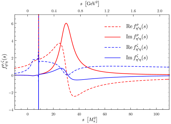
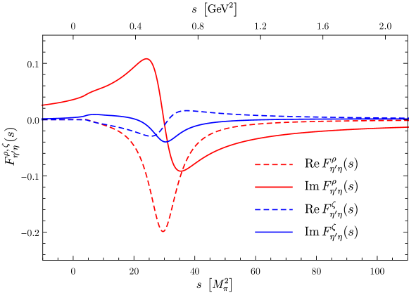
3.2.1 $\eta\to\pi^{0}\gamma^{\ast}$

The basis solutions for the $P$-wave amplitude $f_{\eta\pi}$ are defined by

$$f^{\varepsilon}_{\eta\pi}(s)\equiv\left.\big{[}\mathcal{G}_{1}(s)+\hat{\mathcal{G}}_{1}(s)\big{]}\right|_{\varepsilon=1}\,,\qquad f^{\vartheta}_{\eta\pi}(s)\equiv\left.\big{[}\mathcal{H}_{1}(s)+\hat{\mathcal{H}}_{1}(s)\big{]}\right|_{\vartheta=1}\,,$$ (54)

and illustrated in Fig.ย 4(top). The dimensionless $f^{\varepsilon}_{\eta\pi}$ corresponds to the isoscalar amplitude $\mathcal{M}_{0}^{\eta\pi}$, while $f^{\vartheta}_{\eta\pi}$ belongs to the isotensor one, i.e., to $\mathcal{M}_{2}^{\eta\pi}$. The partial waves have a singular character at pseudothreshold, i.e., the upper limit in $s$ of the physical region in the $\eta\to\pi^{0}\pi^{+}\pi^{-}$ decay, which is contained in the inhomogeneities describing left-hand-cut contributions to the respective partial wave. Note that the form factor, after performing the dispersion integral over the discontinuity as in Eq.ย (27), is perfectly regular at that point. Based on Eq.ย (54), we can calculate the corresponding basis form factors

$$F^{\nu}_{\eta\pi}(s)=F^{(1)}_{\eta\pi}(s)|_{f_{\eta\pi}=f_{\eta\pi}^{\nu}}\,,\hskip 14.22636pt\mathrm{with}\hskip 14.22636pt\nu\in\{\varepsilon,\vartheta\}\,,$$ (55)

which allow us to linearly decompose $F_{\eta\pi}^{(1)}$ according to

$$F_{\eta\pi}^{(1)}(s)=\varepsilon F_{\eta\pi}^{\varepsilon}(s)+\vartheta F_{\eta\pi}^{\vartheta}(s)\,.$$ (56)

The $F_{\eta\pi}^{\nu}$ are pure predictions of our dispersive representation, independent of the subtraction constants. Our results for the basis solutions for the form factors are depicted in Fig.ย 4(bottom).

Let us have a look at the hierarchy of the two amplitudes contributing to $F_{\eta\pi}^{(1)}$. The plots in Fig.ย 4 show that the basis solutions for the isoscalar and isotensor contributions to the $\eta\to\pi^{0}\pi^{+}\pi^{-}$ $P$-wave amplitude are of the same order of magnitude, and so are, as a result, the corresponding basis form factors. But due to the vast difference in their normalizing subtraction constants, the term $\vartheta F_{\eta\pi}^{\vartheta}(s)$ is negligibly small in comparison to $\varepsilon F_{\eta\pi}^{\varepsilon}(s)$. The origin of this discrepancy is well understoodย Gardner:2019nid ; Akdag:2021efj . The totally antisymmetric combination of $P$-wave single-variable functions in the isoscalar amplitude $\mathcal{M}^{\eta\pi}_{0}$, cf.ย Eq.ย (38), leads to a strong kinematic suppression inside the Dalitz plot; for symmetry reasons alone, the amplitude is required to vanish along the three lines $s=t$, $t=u$, and $u=s$. As a result, the corresponding normalization $\varepsilon$ is far less rigorously constrained from fits to experimental dataย Anastasi:2016cdz than the isotensor amplitude, which only vanishes for $t=u$. No such suppression occurs for the individual partial waves, or the transition form factors, be it in the $\rho$-resonance region or below, in the kinematic range relevant for the semi-leptonic decays studied here, where isoscalar and isotensor contributions show non-negligible, but moderate corrections to a $\rho$-dominance picture. We also remark that this subtle interplay demonstrates that the model-independent connection between Dalitz plots and transition form factors absolutely requires the use of dispersion-theoretical methodsโ€”a low-energy effective theory such as chiral perturbation theory is insufficient for such extrapolations.

Refer to caption
Refer to caption
Figure 4: Basis solutions for the partial waves and form factors for the $\eta\to\pi^{0}$ transition. The partial-wave amplitudes $f_{\eta\pi}^{\nu}$ from Eq.ย (54) are depicted in the upper panel; the singularity at the pseudothreshold $s=(M_{\eta}-M_{\pi^{0}})^{2}$ is clearly visible. These serve as an input to calculate the basis solutions of the transition form factors $F_{\eta\pi}^{\nu}(s)$ as defined in Eq.ย (55) and shown in the lower panel.

For the numerical evaluation of $F^{(1)}_{\eta\pi}$ we only consider the by far dominant source of error, i.e., the uncertainty of the subtraction constants entering the partial wave. As their errors are of the same order of magnitude as their corresponding central values, it is a good approximation to neglect all other sources of uncertainties, such as the variation of phase-shift input.
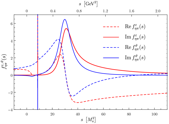
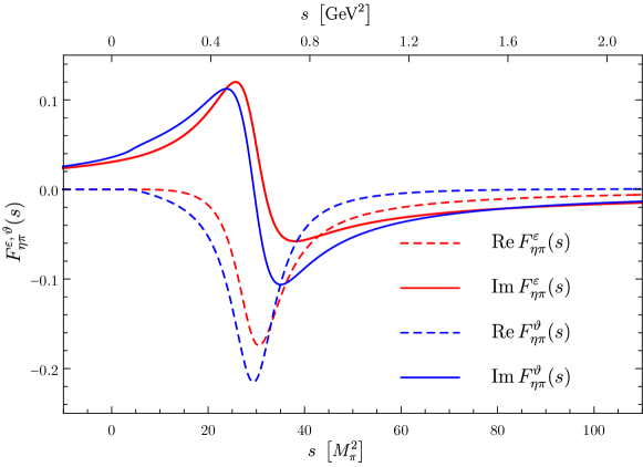
3.2.2 $\eta^{\prime}\to\eta\gamma^{\ast}$

We now turn the focus on the transition form factor $f_{\eta^{\prime}\eta}$, whose basis solutions in terms of partial waves are defined as

$$f^{\varrho}_{\eta^{\prime}\eta}(s)=\left.\big{[}\mathcal{G}_{\pi\pi}(s)+\hat{\mathcal{G}}_{\pi\pi}(s)\big{]}\right|_{\varrho=1,\,\zeta=0}\,,\qquad f^{\zeta}_{\eta^{\prime}\eta}(s)=\left.\big{[}\mathcal{G}_{\pi\pi}(s)+\hat{\mathcal{G}}_{\pi\pi}(s)\big{]}\right|_{\varrho=0,\,\zeta=1}\,.$$ (57)

Using the $f^{\nu}_{\eta^{\prime}\eta}$ we can define the basis from factors

$$F^{\nu}_{\eta^{\prime}\eta}(s)=F^{(1)}_{\eta^{\prime}\eta}(s)|_{f_{\eta^{\prime}\eta}=f_{\eta^{\prime}\eta}^{\nu}}\,,\hskip 14.22636pt\mathrm{with}\hskip 14.22636pt\nu\in\{\varrho,\zeta\}\,,$$ (58)

and finally obtain the complete isovector form factor in explicit dependence on the subtraction constants by means of

$$F^{(1)}_{\eta^{\prime}\eta}(s)=\varrho F_{\eta^{\prime}\eta}^{\varrho}(s)+\zeta F_{\eta^{\prime}\eta}^{\zeta}(s)\,.$$ (59)

The basis solutions for both partial waves and transition form factors are shown in Fig.ย 5.

Refer to caption
Refer to caption
Figure 5: Basis solutions for the partial waves and form factors for the $\eta^{\prime}\to\eta$ transition. The partial-wave amplitudes $f_{\eta^{\prime}\eta}^{\nu}$ from Ref.ย Akdag:2021efj are depicted in the upper panel; again, the singularity at the pseudothreshold $s=(M_{\eta^{\prime}}-M_{\eta})^{2}$ can be seen. These serve as an input to calculate the basis solutions of the transition form factors $F_{\eta^{\prime}\eta}^{\nu}(s)$ as defined in Eq.ย (58) and shown in the lower panel.

3.3 Resonance couplings from analytic continuation

As both the partial waves $f_{XY}(s)$ and the resulting transition form factors $F^{(1)}_{XY}(s)$ have been constructed with the correct analytic properties, we can analytically continue them into the complex plane and onto the second Riemann sheet to extract resonance pole residues. The resonance in question is the $\rho(770)$; its residues can be interpreted as model-independent definitions of $C$-violating $\rho\to XY$ coupling constants. To this end, we recapitulate aspects of Refs.ย Moussallam:2011zg ; Hoferichter:2017ftn . First, consider the discontinuity of the transition form factor in Eq.ย (24) on the first Riemann sheet

$$F^{(1),\,\text{I}}_{XY}(s+i\epsilon)-F^{(1),\,\text{I}}_{XY}(s-i\epsilon)=\frac{i}{24\pi}\big{(}\sigma^{\pi}(s+i\epsilon)\big{)}^{3}\,\big{(}F_{\pi}^{V,\,\text{I}}(s+i\epsilon)\big{)}^{\ast}\,f^{\text{I}}_{XY}(s+i\epsilon),$$ (60)

with

$$\sigma^{\pi}(s)\equiv\sqrt{\frac{4M_{\pi}^{2}}{s}-1}\,,\qquad\sigma^{\pi}(s\pm i\epsilon)=\mp i\,\sigma_{\pi}(s)\,.$$ (61)

Using that the pion vector form factor fulfills Schwarzโ€™ reflection principle and demanding continuity of the scattering amplitudes when moving from one Riemann sheet to another, i.e.,

$$F^{(1),\,\text{I}}_{XY}(s-i\epsilon)=F^{(1),\,\text{II}}_{XY}(s+i\epsilon)\hskip 14.22636pt\mathrm{and}\hskip 14.22636ptF_{\pi}^{V,\,\text{I}}(s-i\epsilon)=F_{\pi}^{V,\,\text{II}}(s+i\epsilon),$$ (62)

we obtain

$$F^{(1),\,\text{II}}_{XY}(s+i\epsilon)=F^{(1),\,\text{I}}_{XY}(s+i\epsilon)-\frac{i}{24\pi}\big{(}\sigma^{\pi}(s+i\epsilon)\big{)}^{3}\,F_{\pi}^{V,\,\text{II}}(s+i\epsilon)\,f^{\text{I}}_{XY}(s+i\epsilon)\,.$$ (63)

In the vicinity of the $\rho(770)$ pole, the transition form factors as well as the pion form factor on the second Riemann sheet behave as

$$F^{(1),\,\text{II}}_{XY}(s)\,,\ F_{\pi}^{V,\,\text{II}}(s)\propto\frac{1}{s_{\rho}-s}\,,\hskip 14.22636pt\mathrm{with}\hskip 14.22636pts_{\rho}=\left(\tilde{M}_{\rho}-i\frac{\Gamma_{\rho}}{2}\right)^{2}.$$ (64)

The pole position $s_{\rho}$ has been determined most accurately in Ref.ย Garcia-Martin:2011nna , using Roy-like equations for pionโ€“pion scattering: $\tilde{M}_{\rho}=763.7\,\text{MeV}$, $\Gamma_{\rho}=146.4\,\text{MeV}$ (cf.ย also Ref.ย Colangelo:2001df ); for later use, we also quote the coupling constant to $\pi\pi$, $|g_{\rho\pi\pi}|=6.01$, ๐š๐ซ๐ โก(๐’ˆ๐†โ€‹๐…โ€‹๐…)=โˆ’5.3โˆ˜subscript๐’ˆ๐†๐…๐…superscript5.3\arg(g_{\rho\pi\pi})=-5.3^{\circ}. We neglect the uncertainties in these parameters, as they are small compared to the ones fixing the partial waves $f_{XY}$. While $F_{\pi}^{V,\,\text{II}}$ is explicitly given in Ref.ย Hoferichter:2017ftn , we can match $F^{(1),\,\text{II}}_{XY}$ to a VMD-type form factor similar to Eq.ย (35), but with $g_{\rho YX}$, $g_{\rho\gamma}$, and $M^{2}_{\rho}$ instead of $\tilde{g}$, $g_{v\gamma}$, and $M^{2}_{v}$. Thus, in sufficient vicinity to the pole, we can write

$$F_{\pi}^{V,\,\text{II}}(s)=\frac{g_{\rho\pi\pi}}{g_{\rho\gamma}}\frac{s_{\rho}}{s_{\rho}-s}\hskip 14.22636pt\mathrm{and}\hskip 14.22636ptF^{(1),\,\text{II}}_{XY}(s)=\frac{g_{\rho YX}}{2g_{\rho\gamma}}\frac{M^{2}_{\rho}}{s_{\rho}-s}.$$ (65)

If we evaluate Eq.ย (63) near the pole $s_{\rho}$ and insert Eq.ย (65), we can compute the desired $C$-odd $\rho$-meson couplings by

$\displaystyle g_{\rho YX}$ $\displaystyle=\frac{g_{\rho\pi\pi}}{12\pi}\frac{s_{\rho}}{M^{2}_{\rho}}\sigma^{3}_{\pi}(s_{\rho})\,f^{\text{I}}_{XY}(s_{\rho})\,.$ (66)
\@afterheading

The problem is therefore reduced to evaluating the partial wave $f^{\text{I}}_{XY}$ on the first Riemann sheet at the pole position, a task for which the dispersive representations are perfectly suited. To clarify the dependence on subtractions or effective coupling constants and therefore separate the uncertainty in these from the precisely calculable dispersive aspects, we will once more make use of the decomposition in terms of basis functions.

We begin with the $\eta\to\pi^{0}$ transition form factor. The basis functions of the partial wave $f_{\eta\pi}$, evaluated at the $\rho$ pole, result in

$$f_{\eta\pi}^{\varepsilon}(s_{\rho})=-0.02-2.76i\,,\qquad f_{\eta\pi}^{\vartheta}(s_{\rho})=0.87-3.05i\,,$$ (67)

so that we obtain

$$f_{\eta\pi}(s_{\rho})=\varepsilon f_{\eta\pi}^{\varepsilon}(s_{\rho})+\vartheta f_{\eta\pi}^{\vartheta}(s_{\rho})=\big{[}(-0.704+i\,0.005)\,\text{GeV}^{4}\,g_{0}-(1.149+i\,0.330)g_{2}\big{]}\,,$$ (68)

where we made use of Eq.ย (44). Employing of Eq.ย (66) and finally inserting the values for the coupling constants $g_{0}$ and $g_{2}$ as extracted from the $\eta\to\pi^{0}\pi^{+}\pi^{-}$ Dalitz-plot asymmetry then yields

$\displaystyle g_{\rho\pi\eta}$ $\displaystyle=\big{[}(-0.087+i\,0.021)\,\text{GeV}^{4}\,g_{0}-(0.151+i\,0.007)\,g_{2}\big{]}$ (69)
$\displaystyle=\big{[}0.24(0.39)-i\,0.06(0.10)\big{]}\,\mathrm{GeV}^{-2}\,.$
\@afterheading

Note that the isotensor contribution $g_{2}$ is negligible in the coupling $g_{\rho\pi\eta}$.

The analytic continuation of the basis partial wave for $f_{\eta^{\prime}\eta}$ to the pole position of the $\rho$ meson yields

$$f_{\eta^{\prime}\eta}^{\varrho}(s_{\rho})=0.44-2.95i\,,\qquad f_{\eta^{\prime}\eta}^{\zeta}(s_{\rho})=-0.45-0.17i\,.$$ (70)

With Eq.ย (52) we can hence express the analytically continued partial wave at the $\rho$ pole by

$$f_{\eta^{\prime}\eta}(s_{\rho})=\varrho f_{\eta^{\prime}\eta}^{\varrho}(s_{\rho})+\zeta f_{\eta^{\prime}\eta}^{\zeta}(s_{\rho})=g_{1}\left[(0.12-i\,0.34)+(1.63+i\,0.48)\,\text{GeV}^{2}\,\delta g_{1}\right]\,.$$ (71)

In terms of this result, the $\rho$-meson coupling from Eq.ย (66) results in

$\displaystyle g_{\rho\eta\eta^{\prime}}$ $\displaystyle=g_{1}\left[(0.005-i\,0.046)+(0.215+i\,0.011)\,\text{GeV}^{2}\,\delta g_{1}\right]$ (72)
$\displaystyle=-\big{[}0.82(2.25)+i\,0.07(0.16)\big{]}\,\mathrm{GeV}^{-2}\,,$
\@afterheading

where we considered correlated Gaussian errors for the couplings $g_{1}$ and $\delta g_{1}$.

Note that the coupling constants in Eq.ย (66) become inevitably complex-valued, thus spoiling the well-defined transformation under time reversal when compared to the tree-level coupling constants from ToPe$\chi$PT. This is neither surprising nor specific to the context of symmetry violation studied here: in the strong interactions, resonance couplings that are real in the narrow-width limit necessarily turn complex when defined model-independently via pole residues in the complex plane. However, this points towards the reason why these complex phases will be irrelevant when using symmetry arguments to estimate isoscalar contributions in the next section: for the narrow $\omega$ and $\phi$ resonances, they are negligible to far better accuracy; symmetry arguments within the vector-meson nonet are not applicable to their total widths. We will therefore simply omit the imaginary parts in the next section and relate the $C$-odd $\omega$ couplings required for the model of the isoscalar parts of the form factors to the real parts of the $\rho$ coupling (of the same total isospin) only. Note furthermore that Eqs.ย (69) and (72) still suggest the imaginary parts of $g_{\rho\pi\eta}$ and $g_{\rho\eta\eta^{\prime}}$ to be rather small, such that the difference between real part and modulus, e.g., is negligible for our purposes.

4 Hadronic long-range effects: the isoscalar contribution

We now attempt to combine the findings of Sects.ย 2.4.2 andย 3.3. We wish to access the couplings $\tilde{g}$, cf.ย Eq.ย (35), by linking them to the $g_{\rho YX}$ discussed in the last section. In Sect.ย 2.4.2 we found a ToPe$\chi$PT operator that, when considered separately, allows usโ€”according to Eq.ย (LABEL:eq:correlated_couplings)โ€”to relate these couplings by $SU(3)$ symmetry. The vector-meson couplings with the same total isospin are found to be related by $g_{\omega\pi\eta}=1/\sqrt{3}\,g_{\rho\eta\eta^{\prime}}$ and $g_{\omega\eta\eta^{\prime}}=\sqrt{3}\,g_{\rho\pi\eta}$, while $g_{\phi\pi\eta}=0$ and $g_{\phi\eta\eta^{\prime}}$ does not correlate with respective $\rho$ couplings. However, the predictive power of flavor symmetry arguments does not hold in general for all operators. This leads to the shortcoming that we cannot fix the relative sign of the couplings, which becomes evident when comparing Eqs.ย (LABEL:eq:uncorrelated_couplings) and (LABEL:eq:correlated_couplings), and have to rely on NDA arguments to consider that there may be additional contributions to the couplings from linear combinations of Wilson coefficients, cf.ย Eq.ย (LABEL:eq:uncorrelated_couplings). An alternative approach would be to use NDA right away and drop the relative factors of $1/\sqrt{3}$ and $\sqrt{3}$, respectively, but this still leads to the same caveats.

4.1 $\eta\to\pi\ell^{+}\ell^{-}$

Possible contributions to the isoscalar form factor in $\eta\to\pi^{0}\ell^{+}\ell^{-}$ can originate from an $\omega$ or a $\phi$ intermediate state. In accordance with Sect.ย 2.4.2, these enter the form factor in the linear combination

$$F_{\eta\pi}^{(0)}(s)\equiv\frac{g_{\omega\pi\eta}}{2g_{\omega\gamma}}\frac{M^{2}_{\omega}}{M^{2}_{\omega}-s}+\frac{g_{\phi\pi\eta}}{2g_{\phi\gamma}}\frac{M^{2}_{\phi}}{M^{2}_{\phi}-s}\,.$$ (73)

With our $SU(3)$ estimate $g_{\phi\pi\eta}=0$ we can ignore the contribution of the $\phi$. Dropping the latter is also justified from an NDA point of view: the difference of the two summands in Eq.ย (73) is negligible compared to the uncertainty of NDA if $F_{\eta\pi}^{(0)}(s)$ is evaluated within the physical range. Therefore, we continue the estimation of the isoscalar contribution with the $\omega$ intermediate state only, for which we use $|g_{\omega\gamma}|=16.7(2)$ย Hoferichter:2017ftn .

Relating $g_{\omega\pi\eta}$ to the $\rho$ coupling of the same total isospin $I=1$ and omitting the imaginary part for the reasons given above, we find

$$g_{\omega\pi\eta}\approx\frac{1}{\sqrt{3}}\text{Re}\,g_{\rho\eta\eta^{\prime}}=-0.47(1.30)\,\mathrm{GeV}^{-2}\hskip 14.22636pt\mathrm{or}\hskip 14.22636pt|g_{\omega\pi\eta}|\lesssim 1.8\,\mathrm{GeV}^{-2}\,.$$ (74)

Throughout this manuscript we do not account for the numerically intangible uncertainties from our $SU(3)$ estimates or NDA. As neither of the latter fixes the sign of $|g_{\omega\pi\eta}|$, we have to content ourselves with its absolute value. Note that retaining the imaginary part of $g_{\rho\eta\eta^{\prime}}$ would have a negligible effect on the upper limit for $|g_{\omega\pi\eta}|$.

On the other hand, we can also place a bound on $|g_{\omega\pi\eta}|$ using the upper limit on the branching ratio of $\omega\to\eta\pi^{0}$ as determined by the Crystal Ball multiphoton spectrometer at the Mainz Microtron (MAMI)ย Starostin:2009zz and the Lagrangian in Eq.ย (29). The partial decay width is found to be

$$\Gamma(\omega\rightarrow\eta\pi^{0})=\frac{1}{192\pi M_{\omega}}\,|g_{\omega\pi\eta}|^{2}\,\lambda^{3/2}\big{(}M_{\omega}^{2},M_{\eta}^{2},M_{\pi^{0}}^{2}\big{)}\,.$$ (75)

With $\text{BR}(\omega\rightarrow\eta\pi^{0})<2.3\cdot 10^{-4}$ย Starostin:2009zz and $\Gamma_{\omega}=8.68$ย MeVย Workman:2022ynf , we obtain the bound

$$|g_{\omega\pi\eta}|<0.24\,\mathrm{GeV}^{-2}\,,$$ (76)

which is significantly more restrictive than the theoretical estimate for the bound on the coupling inferred from $g_{\rho\eta\eta^{\prime}}$.

4.2 $\eta^{\prime}\to\eta\ell^{+}\ell^{-}$

Similarly to the previous section, the isoscalar part of the form factor in $\eta^{\prime}\to\eta\ell^{+}\ell^{-}$ can be written as

$$F_{\eta^{\prime}\eta}^{(0)}(s)\equiv\frac{g_{\omega\eta\eta^{\prime}}}{2g_{\omega\gamma}}\frac{M^{2}_{\omega}}{M^{2}_{\omega}-s}+\frac{g_{\phi\eta\eta^{\prime}}}{2g_{\phi\gamma}}\frac{M^{2}_{\phi}}{M^{2}_{\phi}-s}\,.$$ (77)

With the same reasoning as above we henceforth drop the contribution of the $\phi$ and only take the $\omega$ into account. The numerical result for the corresponding vector meson coupling, which has total isospin $I=0$, is

$$g_{\omega\eta\eta^{\prime}}\approx\sqrt{3}\,\text{Re}\,g_{\rho\pi\eta}=0.42(0.68)\,\mathrm{GeV}^{-2}\hskip 14.22636pt\mathrm{or}\hskip 14.22636pt|g_{\omega\eta\eta^{\prime}}|\lesssim 1.1\,\mathrm{GeV}^{-2}\,.$$ (78)

Once more, the imaginary part of $g_{\rho\pi\eta}$ would yield just a minor contribution to the upper limit on $|g_{\omega\eta\eta^{\prime}}|$ and can be neglected. We furthermore remark that the $\rho\pi\eta$ coupling also has an isotensor component, which, however, has a negligible effect, cf.ย Eq.ย (69).

5 Results

With the theoretical apparatus at hand we are now able to predict upper limits on the decay widths

$$\Gamma(X\to Y\ell^{+}\ell^{-})=\frac{\alpha^{2}}{8\pi M_{X}^{3}}\,\int_{4m_{\ell}^{2}}^{(M_{X}-M_{Y})^{2}}\!\text{d}s\,\lambda^{3/2}\big{(}s,M_{X}^{2},M_{Y}^{2}\big{)}\,\sigma_{\ell}(s)\left(1-\frac{\sigma^{2}_{\ell}(s)}{3}\right)|F_{XY}(s)|^{2}\,,$$ (79)

relying on the Dalitz-plot asymmetries in $X\to Y\pi^{+}\pi^{-}$ as the main input. As argued in Sect.ย 2.5, we focus on the long-range contributions via hadronic intermediate states only, i.e., we set

$$F_{XY}(s)=F^{(1)}_{XY}(s)+F^{(0)}_{XY}(s)\,.$$ (80)

We disregard the contributions analyzed in Sects.ย 2.2 and 2.3 according to the discussion in Sect.ย 2.5: these do not show interesting correlations with other ToPe processes, and absent significant cancellations, we can study the consequences of limit setting for the long-range hadronic effects alone. The corresponding transition form factors for the isovector and isoscalar contributions to $\eta\to\pi^{0}\gamma^{\ast}$ read

$\displaystyle F_{\eta\pi}^{(1)}(s)=\varepsilon F_{\eta\pi}^{\varepsilon}(s)+\vartheta F_{\eta\pi}^{\vartheta}(s)\,,\qquad F_{\eta\pi}^{(0)}(s)=\frac{g_{\omega\pi\eta}}{2g_{\omega\gamma}}\frac{M_{\omega}^{2}}{M^{2}_{\omega}-s}\,,$ (81)
\@afterheading

while the ones contributing to $\eta^{\prime}\to\eta\gamma^{\ast}$ are

$\displaystyle F^{(1)}_{\eta^{\prime}\eta}(s)=\varrho F_{\eta^{\prime}\eta}^{\varrho}(s)+\zeta F_{\eta^{\prime}\eta}^{\zeta}(s)\,,\qquad F^{(0)}_{\eta^{\prime}\eta}(s)=\frac{g_{\omega\eta\eta^{\prime}}}{2g_{\omega\gamma}}\frac{M^{2}_{\omega}}{M^{2}_{\omega}-s}\,.$ (82)
\@afterheading

The subtraction constants fixing the $F^{(1)}_{XY}$ are given in Eqs.ย (43) and (51), the respective basis solutions $F_{XY}^{\nu}$ are depicted in Figs.ย 4 andย 5, and the coupling constants $g_{\omega YX}$ entering the $F^{(0)}_{XY}$ are quoted in Eqs.ย (76) and (78), respectively.

We have pointed out above that we have no means to assess the relative sign of the isoscalar contribution. To determine theoretical upper bounds, we therefore employ

$$|F_{\eta\pi}|^{2}\leq|F_{\eta\pi}^{(0)}|^{2}+|F_{\eta\pi}^{(1)}|^{2}+2\,|F_{\eta\pi}^{(0)}|\,|F_{\eta\pi}^{(1)}|$$ (83)

and similarly for $F_{\eta^{\prime}\eta}$, which possibly overestimates the interference term.

5.1 $\eta\to\pi\ell^{+}\ell^{-}$

Refer to caption
Refer to caption
Figure 6: Spectrum of the isovector contribution to the form factor (top) and the corresponding differential decay distribution (bottom) for $\eta\to\pi^{0}\ell^{+}\ell^{-}$. The dashed lines mark the respective upper and lower limits stemming from the uncertainties of the subtraction constants in Eq.ย (43). The physical ranges are in both cases restricted by $4m_{\ell}^{2}\leq s\leq(M_{\eta}-M_{\pi})^{2}$.

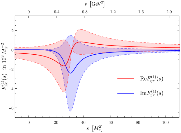
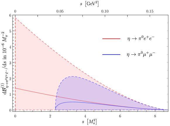
We depict the isovector contributions to the respective form factors and differential decay widths for the decay $\eta\to\pi\ell^{+}\ell^{-}$ in Fig.ย 6. Integrating the region enclosed by the error bands of the differential decay distribution, we obtain the limits

$\displaystyle\mathcal{B}_{\eta\to\pi^{0}e^{+}e^{-}}^{(1)}$ $\displaystyle<20\cdot 10^{-6},$ $\displaystyle\mathcal{B}_{\eta\to\pi^{0}e^{+}e^{-}}$ $\displaystyle<29\cdot 10^{-6},$ $\displaystyle\mathcal{B}_{\eta\to\pi^{0}e^{+}e^{-}}^{\text{exp}}$ $\displaystyle<7.5\cdot 10^{-6}\,,$
$\displaystyle\mathcal{B}_{\eta\to\pi^{0}\mu^{+}\mu^{-}}^{(1)}$ $\displaystyle<7.2\cdot 10^{-6},$ $\displaystyle\mathcal{B}_{\eta\to\pi^{0}\mu^{+}\mu^{-}}$ $\displaystyle<10\cdot 10^{-6},$ $\displaystyle\mathcal{B}_{\eta\to\pi^{0}\mu^{+}\mu^{-}}^{\text{exp}}$ $\displaystyle<5\cdot 10^{-6}\,,$ (84)

where the first entry in each line corresponds to the isovector contribution and the second includes the isoscalar one in addition. Finally, the experimental resultsย WASA-at-COSY:2018jdv ; Dzhelyadin:1980ti , to be understood at 90% C.L., are quoted last, which are of similar order of magnitude as our findings. This observation shows that the considered experiments for $\eta\to\pi^{0}\pi^{+}\pi^{-}$ and $\eta\to\pi^{0}\ell^{+}\ell^{-}$ have a very similar sensitivity for ToPe forces, despite the fact that asymmetries in the former are based on $C$-odd interferences and therefore scale linearly with a (small) BSM couplingย Gardner:2019nid ; Akdag:2022sbn , while the latter is a rate that is suppressed to second order in a similar coupling. Comparing $\mathcal{B}_{\eta\to\pi^{0}\ell^{+}\ell^{-}}^{(1)}$ to $\mathcal{B}_{\eta\to\pi^{0}\ell^{+}\ell^{-}}$, our analysis suggests that the isoscalar form factor contributes roughly one third to the overall branching ratio, however again with the caveat of the imprecise NDA normalization of $F_{\eta\pi}^{(0)}$.

As the experimental limits turn out to be more restrictive than our theoretical predictions for $\mathcal{B}_{\eta\to\pi^{0}\ell^{+}\ell^{-}}^{(1)}$, the $\eta\to\pi^{0}\ell^{+}\ell^{-}$ decay widthsย WASA-at-COSY:2018jdv ; Dzhelyadin:1980ti can be used to refine the fit to the $\eta\to\pi^{0}\pi^{+}\pi^{-}$ Dalitz plotย Anastasi:2016cdz . As long as the latter constrains the corresponding BSM couplings in a way that the form factor is dominated by the contribution of $g_{0}$, an improved regression to the full Dalitz plot is redundant. Instead we note that isoscalar ($g_{0}$) and isotensor ($g_{2}$) couplings in $\eta\to\pi^{0}\pi^{+}\pi^{-}$ are nearly uncorrelatedย Akdag:2021efj and turn the experimental limit for $\mathcal{B}_{\eta\to\pi^{0}e^{+}e^{-}}^{(1)}$ into the upper bound

$$|g_{0}|<4.4\,\text{GeV}^{-6},$$ (85)

to be compared to the previous constraint $g_{0}=-2.8(4.5)\,\text{GeV}^{-6}$ย Akdag:2021efj .

5.2 $\eta^{\prime}\to\eta\ell^{+}\ell^{-}$

Proceeding in analogy to Sect.ย 5.1, we obtain the following upper limits on the decays $\eta^{\prime}\to\eta\ell^{+}\ell^{-}$ (the experimental onesย CLEO:1999nsy ; Dzhelyadin:1980ti again to be understood at 90% C.L.):444For these branching ratios we use the total width $\Gamma_{\eta^{\prime}}=0.23\,\text{MeV}$ listed as PDG average in Ref.ย Workman:2022ynf .

$\displaystyle\mathcal{B}_{\eta^{\prime}\to\eta e^{+}e^{-}}^{(1)}$ $\displaystyle<4.1\cdot 10^{-6},$ $\displaystyle\mathcal{B}_{\eta^{\prime}\to\eta e^{+}e^{-}}$ $\displaystyle<9.0\cdot 10^{-6},$ $\displaystyle\mathcal{B}_{\eta^{\prime}\to\eta e^{+}e^{-}}^{\text{exp}}$ $\displaystyle<2.4\cdot 10^{-3}\,,$
$\displaystyle\mathcal{B}_{\eta^{\prime}\to\eta\mu^{+}\mu^{-}}^{(1)}$ $\displaystyle<1.6\cdot 10^{-6},$ $\displaystyle\mathcal{B}_{\eta^{\prime}\to\eta\mu^{+}\mu^{-}}$ $\displaystyle<3.8\cdot 10^{-6},$ $\displaystyle\mathcal{B}_{\eta^{\prime}\to\eta\mu^{+}\mu^{-}}^{\text{exp}}$ $\displaystyle<15\cdot 10^{-6}\,.$ (86)

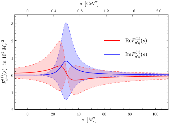
A depiction of the isovector contribution to the form factor and differential decay width is given in Fig.ย 7.

Refer to caption
Refer to caption
Figure 7: Spectrum of the isovector contribution to the form factor (top) and the corresponding differential decay distribution (bottom) for $\eta^{\prime}\to\eta\ell^{+}\ell^{-}$. The dashed lines mark the respective upper and lower limits stemming from the uncertainties of the subtraction constants in Eq.ย (51). The physical ranges are in both cases restricted by $4m_{\ell}^{2}\leq s\leq(M_{\eta^{\prime}}-M_{\eta})^{2}$.

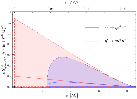
For these decays, our approximation for the isoscalar form factor loosens the limit on the isovector contribution alone by roughly a factor of 2. In contrast to the findings for $\mathcal{B}_{\eta\to\pi^{0}\ell^{+}\ell^{-}}$, our limits on $\mathcal{B}_{\eta^{\prime}\to\eta\ell^{+}\ell^{-}}$ are more restrictive than the respective experimental ones.

6 Summary and outlook

In this work, we have studied the $C$- and $CP$-violating decays $\eta\to\pi^{0}\ell^{+}\ell^{-}$ and $\eta^{\prime}\to\eta\ell^{+}\ell^{-}$, which canโ€”from a phenomenological point of viewโ€”be driven by three different mechanisms. The first two of these are short-distance contributions induced by semi-leptonic four-point vertices and long-distance contributions caused by $C$- and $CP$-odd photonโ€“hadron couplings. The only statements we can make about them is that they contribute as constants to respective transition form factors at leading order in ToPe$\chi$PTย Akdag:2022sbn , that they cannot be distinguished by a sole measurement of the semi-leptonic decay widths, and that NDA estimates them to be of the same order of magnitude.

In contrast, the third mechanism, i.e., long-distance contributions induced by hadronic intermediate states, is conceptually more insightful. To access these contributions we have established dispersion relations for the isovector contribution to the transition form factors $\eta(\to\pi^{0}\pi^{+}\pi^{-})\to\pi^{0}\gamma^{*}$ and $\eta^{\prime}(\to\eta\pi^{+}\pi^{-})\to\eta\gamma^{*}$. By construction, these form factors meet the fundamental requirements of analyticity and unitarity, solely relying on the dominant hadronic contribution of the $P$-waves in the $C$- and $CP$-odd $\eta\to\pi^{0}\pi^{+}\pi^{-}$ and $\eta^{\prime}\to\eta\pi^{+}\pi^{-}$ amplitudes, which have been worked out in Ref.ย Akdag:2021efj . The non-perturbative predictions thereby obtained allow us to directly investigate the correlation between $C$-violating signals in different decays in a model-independent manner. By an analytic continuation of the $C$-odd $\eta\to\pi^{0}\pi^{+}\pi^{-}$ and $\eta^{\prime}\to\eta\pi^{+}\pi^{-}$ $P$-wave amplitudes to the second Riemann sheet, we have extracted $C$-odd $\rho$-meson couplings to $\eta\pi^{0}$ and $\eta^{\prime}\eta$. Furthermore, the latter can be related by total isospin and NDA to coupling constants entering the isoscalar contribution in a VMD model for $\eta^{\prime}\to\eta\omega\to\eta\gamma^{*}$ and $\eta\to\pi^{0}\omega\to\pi^{0}\gamma^{*}$, respectively.

Accounting for these hadronic long-range effects only, we have predicted the corresponding upper limits on the semi-leptonic decay widths, relying on ToPe forces in the respective purely hadronic three-body decays as input. We observed that the currently most precise measurements of $\eta\to\pi^{0}\ell^{+}\ell^{-}$ and $\eta^{\prime}\to\eta\ell^{+}\ell^{-}$ have a similar sensitivity to ToPe interactions as the measured Dalitz-plot asymmetries in $\eta\to\pi^{0}\pi^{+}\pi^{-}$ and $\eta^{\prime}\to\eta\pi^{+}\pi^{-}$, despite their different scaling with small BSM couplings. As we found the experimental limits for $\eta\to\pi^{0}\ell^{+}\ell^{-}$ to be more restrictive than our theoretically predicted ones, we were able to use the respective transition form factor as a constraint to sharpen the bounds on $C$ย violation in $\eta\to\pi^{0}\pi^{+}\pi^{-}$.

Further perspectives on the decays $\eta\to\pi^{0}\ell^{+}\ell^{-}$ and $\eta^{\prime}\to\eta\ell^{+}\ell^{-}$ could be opened by possible future measurements of the respective Dalitz-plot distributions. This would allow us to investigate actual $C$- and $CP$-odd observables, the Dalitz-plot asymmetries arising from the interference with the respective SM contributions. Such interference effects would, as the asymmetries in the hadronic $\eta$ and $\eta^{\prime}$ decays, scale linearly with BSM couplings, however with likely less advantage in sensitivity due to the strongly suppressed SM amplitudes. Still, due to synergy effects with other BSM searches in these decays, such as for weakly coupled light scalarsย Gan:2020aco , renewed experimental efforts are strongly encouraged.

Acknowledgements.
Financial support by the Avicenna-Studienwerk e.V.ย with funds from the BMBF, as well as by the DFG (CRC 110, โ€œSymmetries and the Emergence of Structure in QCDโ€), is gratefully acknowledged.

References

  • (1) S.ย Gardner and J.ย Shi, Patterns of CP violation from mirror symmetry breaking in the $\eta\to\pi^{+}\pi^{-}\pi^{0}$ Dalitz plot, Phys. Rev. D 101 (2020) 115038 [1903.11617].
  • (2) H.ย Akdag, T.ย Isken and B.ย Kubis, Patterns of C- and CP-violation in hadronic $\eta$ and $\eta$โ€™ three-body decays, JHEP 02 (2022) 137 [Erratum JHEP 12 (2022) 156] [2111.02417].
  • (3) H.ย Akdag, B.ย Kubis and A.ย Wirzba, $C$ and $CP$ violation in effective field theories, JHEP 06 (2023) 154 [2212.07794].
  • (4) J.ย Shi, Theoretical Studies of C and CP Violation in $\eta\to\pi^{+}\pi^{-}\pi^{0}$ Decay, Ph.D. thesis, Kentucky U., 2017. 10.13023/etd.2020.388.
  • (5) S.ย Gardner and J.ย Shi, Leading-dimension, effective operators with $CP$ and $C$ or $P$ violation in Standard Model effective field theory, to be published, 2023.
  • (6) J.J.ย Sakurai, Invariance principles and elementary particles, Princeton University Press (1964).
  • (7) L.ย Gan, B.ย Kubis, E.ย Passemar and S.ย Tulin, Precision tests of fundamental physics with $\eta$ and $\eta^{\prime}$ mesons, Phys. Rept. 945 (2022) 2191 [2007.00664].
  • (8) J.ย Bernstein, G.ย Feinberg and T.D.ย Lee, Possible $C$, $T$ Noninvariance in the Electromagnetic Interaction, Phys. Rev. 139 (1965) B1650.
  • (9) B.ย Barrett, M.ย Jacob, M.ย Nauenberg and T.N.ย Truong, Consequences of $C$-Violating Interactions in $\eta^{0}$ and $X^{0}$ Decays, Phys. Rev. 141 (1966) 1342.
  • (10) C.H.ย Llewellynย Smith, The Decay $\eta\to\pi^{0}e^{+}e^{-}$ with $C$ Conservation, Nuovo Cim. A 48 (1967) 834 [Erratum Nuovo Cim. A 50 (1967) 374].
  • (11) T.P.ย Cheng, C-Conserving Decay $\eta\to\pi^{0}e^{+}e^{-}$ in a Vector-Meson-Dominant Model, Phys. Rev. 162 (1967) 1734.
  • (12) J.ย Smith, $C$-Conserving Decay Modes $\eta\to\pi^{0}e^{+}e^{-}$ and $\eta\to\pi^{0}\mu^{+}\mu^{-}$, Phys. Rev. 166 (1968) 1629.
  • (13) J.N.ย Ng and D.J.ย Peters, Decay of the $\eta$ meson into $\pi{\mu}^{+}{\mu}^{-}$, Phys. Rev. D 46 (1992) 5034.
  • (14) J.N.ย Ng and D.J.ย Peters, Study of $\eta\rightarrow{\pi}^{0}\gamma\gamma$ decay using the quark-box diagram, Phys. Rev. D 47 (1993) 4939.
  • (15) R.ย Escribano and E.ย Royo, A theoretical analysis of the semileptonic decays $\eta^{(\prime)}\rightarrow\pi^{0}l^{+}l^{-}$ and $\eta^{\prime}\rightarrow\eta l^{+}l^{-}$, Eur. Phys. J. C 80 (2020) 1190 [Erratum Eur. Phys. J. C 82 (2022) 743] [2007.12467].
  • (16) H.ย Schรคfer, M.ย Zanke, Y.ย Korte and B.ย Kubis, The semileptonic decays $\eta^{(\prime)}\to\pi^{0}\ell^{+}\ell^{-}$ and $\eta^{\prime}\to\eta\ell^{+}\ell^{-}$ in the standard model, to be published, 2023.
  • (17) R.ย Escribano, E.ย Royo and P.ย Sรกnchez-Puertas, New-physics signatures via CP violation in $\eta^{(\prime)}\to{\pi}^{0}{\mu}^{+}{\mu}^{-}$ and ${\eta}^{\prime}\to{\eta}{\mu}^{+}{\mu}^{-}$ decays, JHEP 05 (2022) 147 [2202.04886].
  • (18) R.I.ย Dzhelyadin etย al., Search for Rare Decays of $\eta$ and $\eta^{\prime}$ Mesons and for Light Higgs Particles, Phys. Lett. B 105 (1981) 239.
  • (19) CLEO collaboration, Search for rare and forbidden $\eta^{\prime}$ decays, Phys. Rev. Lett. 84 (2000) 26 [hep-ex/9907046].
  • (20) WASA-at-COSY collaboration, Search for $C$ violation in the decay $\eta\rightarrow\pi^{0}e^{+}e^{-}$ with WASA-at-COSY, Phys. Lett. B 784 (2018) 378 [1802.08642].
  • (21) L.ย Gan and A.ย Gasparian, Search of new physics via eta rare decays, PoS CD09 (2009) 048.
  • (22) GlueX collaboration, L.ย Gan etย al., โ€œEta Decays with Emphasis on Rare Neutral Modes: The JLab Eta Factory (JEF) Experiment.โ€ https://www.jlab.org/exp_prog/proposals/14/PR12-14-004.pdf, 2014.
  • (23) L.ย Gan, Probes for Fundamental QCD Symmetries and a Dark Gauge Boson via Light Meson Decays, PoS CD15 (2015) 017.
  • (24) GlueX collaboration, L.ย Gan etย al., โ€œUpdate to the JEF proposal.โ€ https://www.jlab.org/exp_prog/proposals/17/C12-14-004.pdf, 2017.
  • (25) REDTOP collaboration, The REDTOP project: Rare Eta Decays with a TPC for Optical Photons, PoS ICHEP2016 (2016) 812.
  • (26) REDTOP collaboration, The REDTOP experiment, 1910.08505.
  • (27) REDTOP collaboration, The REDTOP experiment: Rare $\eta/\eta^{\prime}$ Decays To Probe New Physics, 2203.07651.
  • (28) G.ย Kรถpp, Dispersion calculation of the transition form factor $f_{\pi\omega\gamma}(t)$ with cut contributions, Phys. Rev. D 10 (1974) 932.
  • (29) S.P.ย Schneider, B.ย Kubis and F.ย Niecknig, The $\omega\to\pi^{0}\gamma^{*}$ and $\phi\to\pi^{0}\gamma^{*}$ transition form factors in dispersion theory, Phys. Rev. D 86 (2012) 054013 [1206.3098].
  • (30) I.V.ย Danilkin, C.ย Fernรกndez-Ramรญrez, P.ย Guo, V.ย Mathieu, D.ย Schott, M.ย Shi etย al., Dispersive analysis of $\omega/\phi\to 3\pi,\pi^{0}\gamma$, Phys. Rev. D 91 (2015) 094029 [1409.7708].
  • (31) B.ย Kubis and F.ย Niecknig, Analysis of the $J/\psi\to{\pi}^{0}{\gamma}^{*}$ transition form factor, Phys. Rev. D 91 (2015) 036004 [1412.5385].
  • (32) JPAC collaboration, $\omega\rightarrow 3\pi$ and $\omega\pi^{0}$ transition form factor revisited, Eur. Phys. J. C 80 (2020) 1107 [2006.01058].
  • (33) G.ย Dโ€™Ambrosio, G.ย Ecker, G.ย Isidori and J.ย Portoles, The Decays $K\to\pi l^{+}l^{-}$ beyond leading order in the chiral expansion, JHEP 08 (1998) 004 [hep-ph/9808289].
  • (34) B.ย Kubis and R.ย Schmidt, Radiative corrections in $K\to\pi\ell^{+}\ell^{-}$ decays, Eur. Phys. J. C 70 (2010) 219 [1007.1887].
  • (35) Particle Data Group collaboration, Review of Particle Physics, PTEP 2022 (2022) 083C01.
  • (36) P.ย Sรกnchez-Puertas, $CP$ violation in $\eta$ muonic decays, JHEP 01 (2019) 031 [1810.13228].
  • (37) T.ย Feldmann, Quark structure of pseudoscalar mesons, Int. J. Mod. Phys. A 15 (2000) 159 [hep-ph/9907491].
  • (38) I.B.ย Khriplovich, What do we know about T odd but P even interaction?, Nucl. Phys. B 352 (1991) 385.
  • (39) R.S.ย Conti and I.B.ย Khriplovich, New limits on T odd, P even interactions, Phys. Rev. Lett. 68 (1992) 3262.
  • (40) J.ย Engel, P.H.ย Frampton and R.P.ย Springer, Effective Lagrangians and parity conserving time reversal violation at low-energies, Phys. Rev. D 53 (1996) 5112 [nucl-th/9505026].
  • (41) M.J.ย Ramsey-Musolf, Electric dipole moments and the mass scale of new T violating, P conserving interactions, Phys. Rev. Lett. 83 (1999) 3997 [Erratum ] [hep-ph/9905429].
  • (42) A.ย Kurylov, G.C.ย McLaughlin and M.J.ย Ramsey-Musolf, Constraints on T odd, P even interactions from electric dipole moments, revisited, Phys. Rev. D 63 (2001) 076007 [hep-ph/0011185].
  • (43) R.ย Omnรจs, On the Solution of certain singular integral equations of quantum field theory, Nuovo Cim. 8 (1958) 316.
  • (44) V.L.ย Chernyak and A.R.ย Zhitnitsky, Asymptotic Behavior of Hadron Form-Factors in Quark Model. (In Russian), JETP Lett. 25 (1977) 510.
  • (45) V.L.ย Chernyak and A.R.ย Zhitnitsky, Asymptotics of Hadronic Form-Factors in the Quantum Chromodynamics. (In Russian), Sov. J. Nucl. Phys. 31 (1980) 544.
  • (46) A.V.ย Efremov and A.V.ย Radyushkin, Asymptotical Behavior of Pion Electromagnetic Form-Factor in QCD, Theor. Math. Phys. 42 (1980) 97.
  • (47) A.V.ย Efremov and A.V.ย Radyushkin, Factorization and Asymptotical Behavior of Pion Form-Factor in QCD, Phys. Lett. B 94 (1980) 245.
  • (48) G.R.ย Farrar and D.R.ย Jackson, The Pion Form-Factor, Phys. Rev. Lett. 43 (1979) 246.
  • (49) G.P.ย Lepage and S.J.ย Brodsky, Exclusive Processes in Quantum Chromodynamics: Evolution Equations for Hadronic Wave Functions and the Form-Factors of Mesons, Phys. Lett. B 87 (1979) 359.
  • (50) G.P.ย Lepage and S.J.ย Brodsky, Exclusive Processes in Perturbative Quantum Chromodynamics, Phys. Rev. D 22 (1980) 2157.
  • (51) H.ย Leutwyler, Electromagnetic form factor of the pion, hep-ph/0212324.
  • (52) B.ย Ananthanarayan, I.ย Caprini and I.S.ย Imsong, Implications of the recent high statistics determination of the pion electromagnetic form factor in the timelike region, Phys. Rev. D 83 (2011) 096002 [1102.3299].
  • (53) C.ย Hanhart, S.ย Holz, B.ย Kubis, A.ย Kupล›ฤ‡, A.ย Wirzba and C.-W.ย Xiao, The branching ratio $\omega\rightarrow\pi^{+}\pi^{-}$ revisited, Eur. Phys. J. C 77 (2017) 98 [Erratum Eur. Phys. J. C 78 (2018) 450] [1611.09359].
  • (54) B.ย Lee, Chiral dynamics, Cargese Lect. Phys. 5 (1972) 119.
  • (55) O.ย Kaymakcalan and J.ย Schechter, Chiral Lagrangian of Pseudoscalars and Vectors, Phys. Rev. D 31 (1985) 1109.
  • (56) U.-G.ย MeiรŸner, Low-Energy Hadron Physics from Effective Chiral Lagrangians with Vector Mesons, Phys. Rept. 161 (1988) 213.
  • (57) P.ย Jain, R.ย Johnson, U.-G.ย MeiรŸner, N.W.ย Park and J.ย Schechter, Realistic Pseudoscalar Vector Chiral Lagrangian and Its Soliton Excitations, Phys. Rev. D 37 (1988) 3252.
  • (58) F.ย Klingl, N.ย Kaiser and W.ย Weise, Effective Lagrangian approach to vector mesons, their structure and decays, Z. Phys. A 356 (1996) 193 [hep-ph/9607431].
  • (59) M.ย Mai, U.-G.ย MeiรŸner and C.ย Urbach, Towards a theory of hadron resonances, Phys. Rept. 1001 (2023) 1 [2206.01477].
  • (60) V.ย Bernard, N.ย Kaiser and U.-G.ย MeiรŸner, $\pi\eta$ scattering in QCD, Phys. Rev. D 44 (1991) 3698.
  • (61) B.ย Kubis and S.P.ย Schneider, The Cusp effect in $\eta^{\prime}\to\eta\pi\pi$ decays, Eur. Phys. J. C 62 (2009) 511 [0904.1320].
  • (62) JPAC collaboration, Determination of the pole position of the lightest hybrid meson candidate, Phys. Rev. Lett. 122 (2019) 042002 [1810.04171].
  • (63) N.N.ย Khuri and S.B.ย Treiman, Pionโ€“Pion Scattering and $K^{\pm}\to 3\pi$ Decay, Phys. Rev. 119 (1960) 1115.
  • (64) J.ย Stern, H.ย Sazdjian and N.H.ย Fuchs, What $\pi$-$\pi$ scattering tells us about chiral perturbation theory, Phys. Rev. D 47 (1993) 3814 [hep-ph/9301244].
  • (65) B.ย Ananthanarayan and P.ย Bรผttiker, Comparison of $\pi K$ scattering in SU(3) chiral perturbation theory and dispersion relations, Eur. Phys. J. C 19 (2001) 517 [hep-ph/0012023].
  • (66) M.ย Zdrรกhal and J.ย Novotnรฝ, Dispersive Approach to Chiral Perturbation Theory, Phys. Rev. D 78 (2008) 116016 [0806.4529].
  • (67) G.ย Colangelo, S.ย Lanz, H.ย Leutwyler and E.ย Passemar, Dispersive analysis of $\eta\rightarrow 3\pi$, Eur. Phys. J. C 78 (2018) 947 [1807.11937].
  • (68) BESIII collaboration, Precision measurement of the matrix elements for $\eta\to\pi^{+}\pi^{-}\pi^{0}$ and $\eta\to\pi^{0}\pi^{0}\pi^{0}$ decays, Phys. Rev. D 107 (2023) 092007 [2302.08282].
  • (69) KLOE-2 collaboration, Precision measurement of the $\eta\to\pi^{+}\pi^{-}\pi^{0}$ Dalitz plot distribution with the KLOE detector, JHEP 05 (2016) 019 [1601.06985].
  • (70) I.ย Caprini, G.ย Colangelo and H.ย Leutwyler, Regge analysis of the $\pi\pi$ scattering amplitude, Eur. Phys. J. C 72 (2012) 1860 [1111.7160].
  • (71) T.ย Isken, B.ย Kubis, S.P.ย Schneider and P.ย Stoffer, Dispersion relations for $\eta^{\prime}\rightarrow\eta\pi\pi$, Eur. Phys. J. C 77 (2017) 489 [1705.04339].
  • (72) M.ย Albaladejo and B.ย Moussallam, Form factors of the isovector scalar current and the $\eta\pi$ scattering phase shifts, Eur. Phys. J. C 75 (2015) 488 [1507.04526].
  • (73) J.ย Lu and B.ย Moussallam, The $\pi\eta$ interaction and $a_{0}$ resonances in photonโ€“photon scattering, Eur. Phys. J. C 80 (2020) 436 [2002.04441].
  • (74) BESIII collaboration, Measurement of the matrix elements for the decays $\eta^{\prime}\rightarrow\eta\pi^{+}\pi^{-}$ and $\eta^{\prime}\rightarrow\eta\pi^{0}\pi^{0}$, Phys. Rev. D 97 (2018) 012003 [1709.04627].
  • (75) B.ย Moussallam, Couplings of light $I=0$ scalar mesons to simple operators in the complex plane, Eur. Phys. J. C 71 (2011) 1814 [1110.6074].
  • (76) M.ย Hoferichter, B.ย Kubis and M.ย Zanke, Radiative resonance couplings in $\gamma\pi\to\pi\pi$, Phys. Rev. D 96 (2017) 114016 [1710.00824].
  • (77) R.ย Garcรญa-Martรญn, R.ย Kamiล„ski, J.R.ย Pelรกez and J.ย Ruizย de Elvira, Precise determination of the $f_{0}(600)$ and $f_{0}(980)$ pole parameters from a dispersive data analysis, Phys. Rev. Lett. 107 (2011) 072001 [1107.1635].
  • (78) G.ย Colangelo, J.ย Gasser and H.ย Leutwyler, $\pi\pi$ scattering, Nucl. Phys. B 603 (2001) 125 [hep-ph/0103088].
  • (79) A.ย Starostin etย al., Search for the charge-conjugation-forbidden decay $\omega\to\eta\pi^{0}$, Phys. Rev. C 79 (2009) 065201.