Supplemental Material for:
High-Energy Collision of Quarks and Hadrons in the Schwinger Model:
From Tensor Networks to Circuit QED

This Supplemental Material is organized as follows. In Sec. I, we discuss the Thirring-Schwinger model, a generalization of the Schwinger model studied in the main text. In particular, we derive in perturbation theory the effective quark-antiquark Hamiltonian [Eq. (4) of the main text] and discuss the existence (or lack thereof) of bound states. In Sec. II, we derive a corresponding circuit-QED Hamiltonian and discuss an experimental scheme for wave-packet preparation. In LABEL:sec:numerics, we present the details of the numerical tensor-network methods employed, including uniform matrix product states, wave-packet preparation, and particle detection.

I The Massive Thirring-Schwinger model

In this section, we discuss the massive Thirring-Schwinger model, realized in our circuit-QED proposal, including its bosonization, Hamiltonian formulation, and the presence of quark-antiquark bound states for different parameters.

I.1 Hamiltonian and bosonic dual

Consider the Lagrangian density for the so-called massive Thirring-Schwinger model

$$\mathcal{L}=\bar{\psi}(i\not{\partial}-e\not{A}-m)\psi-\frac{1}{4}F_{\mu\nu}F^{\mu\nu}-\frac{1}{2}g(\bar{\psi}\gamma^{\mu}\psi)(\bar{\psi}\gamma_{\mu}\psi)\,,$$ (S1)

which for $g=0$ reduces to the massive Schwinger model investigated in this study [Eq. (1) in the main text], while $e=0$ yields the massive Thirring model [frohlichMassiveThirringSchwingerModel1976, colemanQuantumSineGordonEquation1975]. The gauge fields can be eliminated using Gauss’s law [colemanMoreMassiveSchwinger1976], which, after fixing the gauge to $A_{1}(x)=0$, reads

$$\partial_{x}E=-\partial_{x}^{2}A_{0}=e\rho,$$ (S2)

where $\rho(x)=\psi^{\dagger}(x)\psi(x)$ is the charge-density operator. The solution to this equation is

$$A_{0}(x)=a_{0}-\frac{e\theta}{2\pi}x-\frac{e}{2}\int dx^{\prime}\,\rho(x^{\prime})|x-x^{\prime}|,$$ (S3)

where $a_{0}$ and $\theta$ are integration constants. As argued in Ref. [colemanMoreMassiveSchwinger1976], physics depends on $\theta$ only modulo $2\pi$, and so a suitable range for this variable is $\theta\in(-\pi,\pi]$. The Hamiltonian can be derived in the standard fashion, noting the expression for the electric field from Eq. S2 with $A_{0}$ given in Eq. S3. In the charge-zero subspace $\int dx\,\rho(x)=0$, the (normal-ordered) Hamiltonian of the Thirring-Schwinger model becomes

$$H= \int dx\,:\psi^{\dagger}\gamma^{0}\left(-i\gamma^{1}\partial_{x}+m\right)\psi:-\frac{e^{2}\theta}{2\pi}\int dx\,x\,:\rho(x):\,$$

$$-\frac{e^{2}}{4}\int dx\int dx^{\prime}\,|x-x^{\prime}|:\rho(x)\rho(x^{\prime}):+\frac{g}{2}\int dx:\left[\rho(x)^{2}-\left(\psi^{\dagger}(x)\gamma^{0}\gamma^{1}\psi(x)\right)^{2}\right]\,.$$ (S4)

Our conventions are such that $\{\gamma^{\mu},\gamma^{\nu}\}=2\eta^{\mu\nu}$, with metric signature $\eta^{00}=-\eta^{11}=+1$. The two-component spinor operators, $\psi(x,t)\equiv(\psi_{1}(x,t),\psi_{2}(x,t))^{T}$, satisfy the canonical anticommutation relations $\{\psi_{a}(x,t),\psi^{\dagger}_{b}(x^{\prime},t)\}=\delta_{ab}\delta(x-x^{\prime})$, where $a,b=1,2$. The model described above can be shown to be dual to a bosonic theory with the Hamiltonian [colemanChargeShieldingQuark1975, colemanMoreMassiveSchwinger1976, frohlichMassiveThirringSchwingerModel1976, colemanQuantumSineGordonEquation1975]

$$H=\int dx\,\left[\frac{\Pi^{2}}{2}+\frac{(\partial_{x}\phi)^{2}}{2}+\frac{M^{2}(\phi+\theta/\beta)^{2}}{2}-u\cos(\beta\phi)\right]\,,$$ (S5)

where $[\phi(x),\Pi(y)]=i\delta(x-y)$ and $[\Pi(x),\Pi(y)]=[\phi(x),\phi(y)]=0$. The model parameters are related to those in the fermionic model as follows:

$$M=\frac{e}{\sqrt{\pi}}\frac{1}{\sqrt{1+{g}/{\pi}}},\quad u=\frac{e^{\gamma}}{2\pi}\Lambda m,\quad\beta=\sqrt{\frac{4\pi}{1+{g}/{\pi}}}\,,$$ (S6)

with $\gamma$ being the Euler’s constant and $\Lambda\gg e,m$ being a UV hard momentum cutoff, see Ref. [colemanQuantumSineGordonEquation1975] for details. Furthermore, the following relation holds between the fermionic current $\overline{\psi}\gamma^{\mu}\psi$ and the bosonic field $\phi$ [colemanQuantumSineGordonEquation1975]:

$$\overline{\psi}\gamma^{\mu}\psi\,=\,-\frac{\beta}{2\pi}\epsilon^{\mu\nu}\partial_{\nu}\phi.$$ (S7)

Here, $\epsilon^{\mu\nu}$ is the Levi-Civita tensor. Now, using $\partial_{x}E=e\overline{\psi}\gamma^{0}\psi$ [see Eq. S2], one arrives at $\frac{e\beta}{2\pi}\phi=E$, which relates the scalar field $\phi$ to the electric field $E$. It is more convenient to work with a shifted $\phi$: $\phi\rightarrow\phi-\theta/\beta$, such that the Hamiltonian is

$$H=\int dx\,\left[\frac{\Pi^{2}}{2}+\frac{(\partial_{x}\phi)^{2}}{2}+\frac{M^{2}\phi^{2}}{2}-u\cos(\beta\phi-\theta)\right]\,,$$ (S8)

and the relation to the electric field is now $\frac{e\beta}{2\pi}\phi=E+\frac{e\theta}{2\pi}\equiv E_{T}$, which in the limit $g=0$ reproduces the relation presented in the main text between the total electric field $E_{T}$ and the bosonic field of the massive Schwinger model. When $g=0$, Eq. S8 reduces to Eq. (2) of the main text. Finally, note that the dimensionless coupling $e/m$ in the fermionic theory corresponds to the combination $\Lambda M/u$ in the bosonic theory [jentschPhysicalPropertiesMassive2022].

I.2 Quark-antiquark interactions and bound states

In this section, we derive an effective quark-antiquark Hamiltonian in the nonrelativistic limit in perturbation theory and use this Hamiltonian to confirm the existence of quark-antiquark bound states (mesons). We also study the meson bound states using nonperturbative tensor-network computation of the low-lying spectrum.

I.2.1 Derivation of effective Hamiltonian

The goal is to derive an effective interaction Hamiltonian between a quark and an antiquark to leading order in the interactions $e$ and $g$. For $g=0$, an analogous computation was discussed by Coleman in Ref. [colemanMoreMassiveSchwinger1976]. The idea is that, in the weak-coupling limit in which $e/m,g\ll 1$, one can restrict the physics to subspaces with fixed particle number, e.g., vacuum, quark-antiquark state, etc. , since transitions between states with different particle numbers are higher order in the coupling strength [colemanMoreMassiveSchwinger1976]. This means that, in this limit, the full Hamiltonian can be assumed to be almost block-diagonal in the Fock basis. This mimics a nonrelativistic limit in which one can define an ‘effective’ potential describing interactions in each fixed-particle sector, with well-defined quantum-mechanical operators $\hat{x}$ and $\hat{p}$ which would have been meaningless otherwise. Relativistic corrections in the dynamics can be included using standard quantum-mechanical perturbation theory, while corrections in the kinematics can be included by incorporating higher-order terms in $p/m$, where $p$ is the typical momentum in the system. Such a notion of an effective Hamiltonian is useful to get a qualitative understanding of the nature of quark-antiparticle interactions in such a limit, and to make analytic predictions for the expected spectrum that can be compared against exact numerics.

To start with, we keep the kinematics relativistic but constrain our analysis to the two-particle sector only. A nonrelativistic expansion in $p/m$ will be performed at the end. First, note that the quadratic piece of the Hamiltonian in Eq. S4, $H_{0}\equiv\int dx\,:\psi^{\dagger}\gamma^{0}\left(-i\gamma^{1}\partial_{x}+m\right)\psi:$, can be diagonalized by a standard mode expansion:

$$\psi_{a}(x)=\int\frac{dk}{\sqrt{4\pi E_{k}}}e^{ikx}\left[u_{a}(k)b(k)+v_{a}(-k)c^{\dagger}(-k)\right],$$ (S9)

where $E_{k}\equiv\sqrt{k^{2}+m^{2}}$ with $k\equiv k^{1}=-k_{1}$, and $u(k)$ and $v(k)$ are two-component spinor wave functions that satisfy the classical Dirac equation for positive and negative frequencies, respectively: $(\not{k}-m)u(k)=(\not{k}+m)v(k)=0$ (here, $\not{k}=E_{k}\gamma^{0}-k\gamma^{1}$). The creation operators for quarks and antiquarks satisfy the canonical anticommutation relations $\{b(k),b^{\dagger}(k^{\prime})\}=\{c(k),c^{\dagger}(k^{\prime})\}=\delta(k-k^{\prime})$. Further, the following representation of Dirac matrices is used for explicit computations, $\gamma^{0}=\sigma^{z}$ and $\gamma^{1}=i\sigma^{y}$, so that the spinor wavefunctions are given by $u(k)=\begin{pmatrix}\sqrt{m+E_{k}}\\ \frac{k}{\sqrt{m+E_{k}}}\end{pmatrix}$ and $v(k)=\begin{pmatrix}\frac{k}{\sqrt{m+E_{k}}}\\ \sqrt{m+E_{k}}\end{pmatrix}$, leading to the free-fermion Hamiltonian

$$H_{0}=\int dk\,E_{k}\left[b^{\dagger}(k)b(k)+c^{\dagger}(k)c(k)\right].$$ (S10)

A quark-antiquark state in the noninteracting limit can be written as

$$|p,q\rangle=b^{\dagger}(p)c^{\dagger}(q)|0\rangle,$$ (S11)

where $|0\rangle$ is the Fock vaccum of $H_{0}$ and where the quark (antiquark) has momentum $p$ ($q$). Following Coleman [colemanMoreMassiveSchwinger1976], one can now define the reduced center-of-mass Hamiltonian as the operator $H_{\mathrm{eff}}$, whose matrix elements in the two-particle sector are given by

$$\langle p^{\prime},q^{\prime}|H|p,-p\rangle=\delta(p^{\prime}+q^{\prime})\langle p^{\prime}|H_{\mathrm{eff}}|p\rangle.$$ (S12)

The effective Hamiltonian $H_{\mathrm{eff}}$ is a function of a conjugate pair of operators $[\hat{x},\hat{p}]=i$, where $\hat{x}$ is the displacement between the quark and the antiquark and $|p\rangle$ is a single-particle momentum eigenstate, $\hat{p}|p\rangle=p|p\rangle$, with normalization $\langle p^{\prime}|p\rangle=\delta(p-p^{\prime})$. In the absence of interactions, one has

$$\langle p^{\prime},q^{\prime}|H_{0}|p,-p\rangle =2\sqrt{m^{2}+p^{2}}\,\delta(p-p^{\prime})\delta(p^{\prime}+q^{\prime})\quad\Rightarrow\quad H_{\mathrm{eff}}=2\sqrt{m^{2}+\hat{p}^{2}}\,.$$ (S13)

To compute $\langle p^{\prime},q^{\prime}|H|p,-p\rangle$ in the interacting case, one can insert Eq. S9 into Eq. S4 to obtain

$$\langle p^{\prime}|H_{\mathrm{eff}}|p\rangle =2\sqrt{m^{2}+p^{2}}\,\delta(p-p^{\prime})-\frac{e^{2}\theta}{4\pi^{2}}\int dx\,x\,e^{i(p-p^{\prime})x}+\frac{e^{2}}{8\pi E_{p^{\prime}}E_{p}}\left(m^{2}+p^{\prime}p+E_{p^{\prime}}E_{p}\right)\int dx\,|x|\,e^{i(p-p^{\prime})x}$$

$$+\frac{e^{2}}{8\pi}\frac{m^{2}}{E_{p^{\prime}}^{2}E_{p}^{2}}-\frac{g}{2\pi E_{p^{\prime}}E_{p}}\left(m^{2}+p^{\prime}p+E_{p^{\prime}}E_{p}\right).$$ (S14)

Note that all interaction terms are of the form

$$\langle p^{\prime}|\hat{O}|p\rangle=f_{1}(p^{\prime})f_{2}(p)\int\frac{dx}{2\pi}\,g(x)\,e^{i(p-p^{\prime})x}$$ (S15)

for some functions $f_{1}$, $f_{2}$, and $g$ [for the last line of Eq. (S14), $g(x)=\delta(x)$]. This allows any interaction term $\hat{O}$ to be written as follows:

$$\hat{O} =\left(\int dp^{\prime}\,|p^{\prime}\rangle\langle p^{\prime}|\right)\hat{O}\left(\int dp\,|p\rangle\langle p|\right)$$

$$=\int dp^{\prime}\int dp\,|p^{\prime}\rangle f_{1}(p^{\prime})f_{2}(p)\int\frac{dx}{2\pi}\,g(x)\,e^{i(p-p^{\prime})x}\langle p|$$

$$=f_{1}(\hat{p})\int dp^{\prime}\int dp\,|p^{\prime}\rangle\left(\int dx\,g(x)\langle p^{\prime}|x\rangle\langle x|p\rangle\right)\langle p|f_{2}(\hat{p})$$

$$=f_{1}(\hat{p})\left(\int dp^{\prime}\,|p^{\prime}\rangle\langle p^{\prime}|\right)g(\hat{x})\left(\int dx\,|x\rangle\langle x|\right)\left(\int dp\,|p\rangle\langle p|\right)f_{2}(\hat{p})$$

$$=f_{1}(\hat{p})g(\hat{x})f_{2}(\hat{p})\,.$$ (S16)

Equation S15 is used in the second equality, and the identity $e^{i(p-p^{\prime})x}=2\pi\langle p^{\prime}|x\rangle\langle x|p\rangle$ is used in the third equality. Finally, the effective Hamiltonian can be written as

$$H_{\mathrm{eff}} =2\left(m^{2}+\hat{p}^{2}\right)^{1/2}-\frac{e^{2}\theta}{2\pi}\hat{x}+\frac{e^{2}}{4}\frac{m}{m^{2}+\hat{p}^{2}}\delta(\hat{x})\frac{m}{m^{2}+\hat{p}^{2}}$$

$$+\frac{e^{2}}{4}\left[|\hat{x}|+\frac{\hat{p}}{\left(m^{2}+\hat{p}^{2}\right)^{1/2}}|\hat{x}|\frac{\hat{p}}{\left(m^{2}+\hat{p}^{2}\right)^{1/2}}+\frac{m}{\left(m^{2}+\hat{p}^{2}\right)^{1/2}}|\hat{x}|\frac{m}{\left(m^{2}+\hat{p}^{2}\right)^{1/2}}\right]$$

$$-g\left[\delta(\hat{x})+\frac{\hat{p}}{\left(m^{2}+\hat{p}^{2}\right)^{1/2}}\delta(\hat{x})\frac{\hat{p}}{\left(m^{2}+\hat{p}^{2}\right)^{1/2}}+\frac{m}{\left(m^{2}+\hat{p}^{2}\right)^{1/2}}\delta(\hat{x})\frac{m}{\left(m^{2}+\hat{p}^{2}\right)^{1/2}}\right]\,.$$ (S17)

The lengthy expression in Eq. S17 can be simplified by considering the nonrelativistic limit. Note that, when momentum and energy are large enough for particle creation, $\langle\hat{p}^{2}\rangle\gtrsim m^{2}$, non-particle-conserving, i.e., inelastic, transitions can occur, and, in such a regime, it is not particularly useful to consider an effective potential between a quark and an antiquark. However, since our interest is in an effective interaction between static or slow-moving quark and antiquark—in particular, for investigating the presence of bound states—the matrix elements between states with different particle numbers will be reduced by kinematic constraints. Note that this limit is only applicable when the dimensionless coupling constants $e/m$ and $g$ are small enough, since large couplings result in binding- or scattering-energy scales large enough to violate these assumptions. Based on this discussion, $H_{\mathrm{eff}}$ can be expanded in $p/m\ll 1$ to obtain a simpler effective Hamiltonian at leading order in $p/m$, $e/m$, and $g$:

$$H_{\mathrm{eff}}=2m+\frac{\hat{p}^{2}}{m}+\frac{e^{2}}{2}\left(|\hat{x}|-\frac{\theta}{\pi}\hat{x}\right)+\frac{e^{2}}{4m^{2}}\delta(\hat{x})-2g\delta(\hat{x}).$$ (S18)

In taking the large-$m$ limit, the dimensionless combination $e/m$ is kept fixed. For the Schwinger model, $g=0$, this gives Eq. (4) in the main text. Note that the electric ($e\neq 0$) and the Thirring ($g\neq 0$) interactions contribute short-range terms which compete with each other. In the confined phase ($\theta\neq\pi$), the linear potential guarantees quark-antiquark bound states, which are the fundamental excitations, regardless of the short-range interactions. However, in the deconfined phase ($\theta=\pi$), quarks are free particles (as long as $x>0$, i.e., the quark is to the left of the antiquark). Here, the presence of bound states depends on the delta-function term in Eq. S18. When $g>g_{c}\equiv\frac{e^{2}}{8m^{2}}$, the delta-function term is negative, giving rise to attractive short-range interactions, implying the existence of at least one bound state. For $g<g_{c}$ (including the $g=0$ case considered in the main text), on the other hand, the delta function is repulsive, prohibiting any bound states from forming.

As a nontrivial check on this expression, consider the Thirring model, $e=0$, which is an integrable quantum field theory whose spectrum is known exactly [Dashen:1975hd, Zamolodchikov:1978xm]. The effective Hamiltonian in this case is simply

$$H_{\mathrm{eff}}=2m+\frac{\hat{p}^{2}}{m}-2g\delta(\hat{x})\,.$$ (S19)

This is a standard problem in introductory quantum mechanics (see e.g., Ref. [griffithsquantum]). For $g>0$, there is a single bound state with energy

$$E_{\mathrm{bound}}=2m\big{(}1-\frac{g^{2}}{2}\big{)}.$$ (S20)

The exact Thirring model with $g>0$ has $N$ bound states, where $N$ is the largest integer smaller than $1+2g/\pi$, and the energy of the $n$th bound state is given by [Dashen:1975hd]

$$E_{n}=2m\sin\left(\frac{n\pi/2}{1+2g/\pi}\right),\quad n=1,2,..,N\,.$$ (S21)

For small $g$, there is a single bound state ($n=1$) with energy given, at leading order in $g$, by Eq. S20.

I.2.2 Numerical verification

To go beyond the perturbative results, we make use of the variational uMPS quasiparticle ansatz [see LABEL:sec:uMPS and LABEL:eq:qp-ansatz] to verify the existence of the bound states. In the deconfined phase, quarks are topological “kinks” [colemanMoreMassiveSchwinger1976], and are numerically described by the topological uMPS ansatz, whereas the mesons, if they exist, would be described by the topologically trivial uMPS ansatz (see LABEL:sec:numerics). The energy minimization of the topological uMPS ansatz yields the quark mass $m_{q}$, and the minimization of the topologically trivial uMPS ansatz returns an energy which we denote $m_{\pi}$. To determine if this corresponds to a meson eigenstate, we plot the ratio $m_{\pi}/m_{q}$ in Fig. S1 as a function of $g$. If the meson exists, that ratio needs to satisfy $m_{\pi}/m_{q}<2$, since the bound-state energy must be below the two-particle continuum beginning at $2m_{q}$. Furthermore, plotting this ratio for different values of the bond dimension $D$ of the uMPS ansatz can signify the existence or absence of the meson. This is because, if the meson exists, its wavefunction will be localized, and so the ansatz energy $m_{\pi}$ should be rather insensitive to $D$ and will quickly converge to the true meson mass as $D$ is increased [haegemanElementaryExcitationsGapped2013].

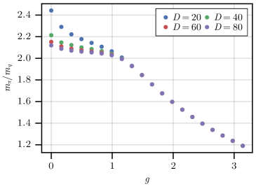
Figure S1: Ratio of the meson mass $m_{\pi}$ to the quark mass $m_{q}$ in the deconfined phase ($\theta=\pi$) as a function of the Thirring interaction strength $g$, for different bond dimensions $D$. The energies are calculated using the variational principle with the uMPS quasiparticle ansatz [see LABEL:eq:qp-ansatz] using the same parameters as in the main text ($\chi=1,\mu^{2}=0.5$, and $\lambda=0.1$).

Figure S1 reveals a critical $g_{c}\approx 1$ (for the parameters used in the main text) above which $m_{\pi}/m_{q}<2$. This region clearly shows insensitivity to $D$, signaling that the ansatz properly captures the nature of the bound-state wave function even for smaller bond dimensions. Below $g_{c}$, on the other hand, $m_{\pi}/m_{q}>2$, and a qualitatively different behavior is observed as a function of $D$, signaling sensitivity to the choice of bond dimension. All this indicates that the bound state in the deconfined phase only exists for sufficiently large $g$, in agreement with the analytical prediction in the previous section. For small $g<g_{c}$, the minimization of the topologically trivial uMPS ansatz results in a two-particle state that is not an eigenstate, but is rather a superposition of many eigenstates from the continuum. The two particles in that state are forced together into a small region of size $\sim\log(D)$, and hence as $D$ is increased, the particles are allowed to spread, which decreases their interaction energy and makes the energy of the variational ansatz approach the bottom of the two-particle band at $2m_{q}$.

II Circuit-QED implementation

In this section, we derive the circuit-QED Hamiltonian from a lumped-element model and present a scheme for preparing meson excitations.

II.1 Hamiltonian derivation

Consider the circuit diagram in LABEL:fig:circuit, which is a more detailed version of Fig. 1 of the main text. Here, each unit cell consists of a capacitor with capacitance $C$, an inductor with inductance $L$, and a Josephson junction with critical current $I_{c}$, in parallel, representing a general rf-SQUID circuit, which includes the fluxonium as a special case [peruzzoGeometricSuperinductanceQubits2021]. Each L-J loop is threaded by an external flux $\Phi_{\mathrm{ext}}$, and different unit cells are coupled together via inductors with inductance $L^{\prime}$. Node fluxes are labeled by $\phi_{i}$, branch fluxes by $\phi_{C}^{i}$, $\phi_{J}^{i}$, and $\phi_{L}^{i}$, for the corresponding elements within node $i$, and the inter-node branch fluxes coupling nodes $i$ and $i+1$ by $\phi_{L^{\prime}}^{i,i+i}$. The branch currents are related to the branch fluxes by $I_{C}^{i}=C\ddot{\phi_{i}}$, $I^{i}_{L}=\phi_{L}^{i}/L$, $I^{i,i+1}_{L^{\prime}}=\phi_{L^{\prime}}^{i,i+1}/L^{\prime}$, and $I_{J}^{i}=I_{c}\sin(\phi_{J}^{i})$, for the capacitor, inductors, and the Josephson junction, respectively .