Exploring new ways: Enforcing representational dissimilarity to learn new features and reduce error consistency

Abstract

Independently trained machine learning models tend to learn similar features. Given an ensemble of independently trained models, this results in correlated predictions and common failure modes. Previous attempts focusing on decorrelation of output predictions or logits yielded mixed results, particularly due to their reduction in model accuracy caused by conflicting optimization objectives. In this paper, we propose the novel idea of utilizing methods of the representational similarity field to promote dissimilarity during training instead of measuring similarity of trained models. To this end, we promote intermediate representations to be dissimilar at different depths between architectures, with the goal of learning robust ensembles with disjoint failure modes. We show that highly dissimilar intermediate representations result in less correlated output predictions and slightly lower error consistency, resulting in higher ensemble accuracy. With this, we shine first light on the connection between intermediate representations and their impact on the output predictions.

1 Introduction

Machine learning methods learn features automatically when trained on a dataset. The high dimensionality of the data should allow for a variety of solutions, yet independent models tend to learn similar features to each other. Many downstream effects of this feature similarity are observed throughout current machine learning literature: a) Geirhos et al. (2020)showed that independently trained CNNs tend to predict erroneously on the same cases much more often than expected by chance given their accuracy, and more often than e.g. humans. b) Csiszárik et al. (2021); Bansal et al. (2021)showed that different models are functionally similar, through stitching (Lenc & Vedaldi, 2015) the top of a model to the bottom of another independently trained model with marginal accuracy penalties. c) Ainsworth et al. (2023)showed that independently trained ResNets exhibit a linear mode connectivity with zero loss barrier, given a previous functionally invariant kernel weight permutation. d) Moschella et al. (2023)showed that distinct latent spaces of two independently trained models tend to differ just by an quasi-isometric transformation.

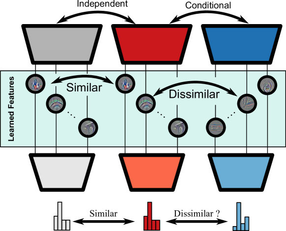
Figure 1: Two independently trained models with different random seed learn very similar features. We propose to train a novel model conditioned on an already trained model with an auxiliary loss enforcing dissimilarity at an intermediate processing stage.

While the feature similarity is not a problem for a single model, multiple models are often combined into an ensemble to improve performance and to measure predictive uncertainty (Lakshminarayanan et al., 2016). When these models learn the same features, they may learn spurious correlations that are not actually useful for the task at hand. This causes them to share failure modes making them fail in the same way. Ensemble improvement is highly dependent on models having a large disagreement error ratio (Theisen et al., 2023) or low error consistency (Geirhos et al., 2020). This can be increased slightly through different augmentation schemes, moderately through different pre-training schemes and strongly through pre-training on a different dataset, with higher error inconsistency in error rates improving ensemble benefits more (Gontijo-Lopes et al., 2022).

Trying to find a new method to increase such predictive diversity between existing models and a new model may become difficult when learning large groups of models, hence methods were introduced that are conditioned on pre-existing models with the intention of learning to solve the task differently.

Early works explored negative correlation (Liu & Yao, 1999a, b; Islam et al., 2003) and evaluated classical methods like boosting or bagging (Dietterich, 2000) for neural networks under the assumption of them being weak classifiers. These approaches suffer great accuracy penalties in modern settings, hence other approaches needed to be developed.

In a more modern setting Pang et al. (2019) trained multiple models simultaneously, enforcing high entropy and orthogonality between the negative class predictions leading to improved adversarial robustness and in-distribution performance of ensembles.

Minderer et al. (2020) proposed a two stage approach for the domain of adversarial learning, first training a model, then learning an augmenting adversarial auto-encoder, that tries to remove the most predictive features while staying as close as possible to the actual image. Given this lens a model can be trained with the lens to learn different features.

So far diversification approaches only regularize inputs or at the position of the output features. However the constraints on regularization at the input and the output are rather large. Adapting input images too much can degrade performance too much and the features at the very end are constrained by having to encode the target classes, constraining the potential solution space models can converge to.

In this paper, we propose to regularize internal representations of a new model to be dissimilar to an existing model to promote discovering novel ways of solving the task, which, to the best of our knowledge, has not been explored so far. Through this we hope to learn about the connection of internal similarity to the predictive behavior between models, specifically whether inducing diversity in intermediate processing stages leads to different predictive behavior and more robust ensembles.

Our main contributions are:

1. We utilize methods from the field of representational similarity in a novel way to train ensembles of very low representational similarity at intermediate layers.

2. We show that highly dissimilar internal representations can be learned at chosen positions with only minor penalties to the model accuracy.

3. We show that enforcing dissimilar internal representations can lead to lower error consistency in the predicted outputs, overall improving ensembling performance relative to an ensemble of independently trained models.

2 Representational (dis)similarity

We are interested in enforcing models to learn different features termed representations, therefore we must define what a representation is. In the field of representational similarity representations z are defined as the input-output responses of all channels of a network’s layer to a set of inputs (Li et al., 2016; Raghu et al., 2017; Morcos et al., 2018; Wang et al., 2018; Kornblith et al., 2019). For a given input batch $x_{i}$ of $B$ samples this results in $\textbf{z}\in\mathcal{R}^{B\times C\times W\times H}$ values for each model.

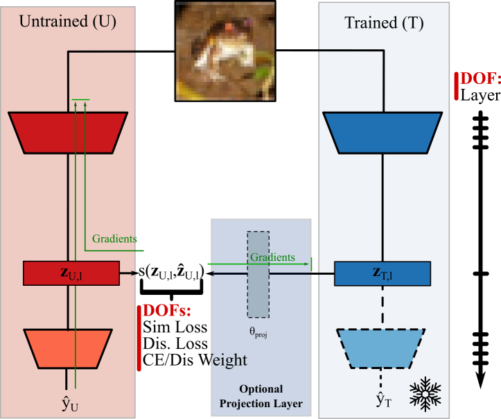
Figure 2: We enforce representational dissimilarity during training of an untrained model (U) given an already trained model (T) through penalizing similarity for U (Eq. 5) and penalizing dissimilarity for T (Eq. 6). As depicted there exist many Degrees of Freedom (DOF) on how to design the system, of which we explore a variety.

Since e.g. the channel dimensions between neurons are not aligned (Li et al., 2016) metrics either need to learn a linear transformation to align representations or use sub-space metrics, e.g. canonical correlation analysis (Raghu et al., 2017; Morcos et al., 2018), to measure similarity. For a nice summary of the differences we refer to Kornblith et al. (2019) and more recently Klabunde et al. (2023).

To formalize: An already trained model $T$ and an untrained model $U$ are composed of $k$ sequential layers $f_{\theta}$ predicting some class probabilities $\hat{y}$, see Eq. 1.

$$\hat{y}_{U,i}=(f_{\theta_{U,k}}\circ\cdots\circ f_{\theta_{U,0}})(x_{i})\\$$ (1)

At some intermediate layer of choice $l$ we collect representations of both models $\textbf{z}_{T,i,l}$ and $\textbf{z}_{U,i,l}$,

$$\textbf{z}_{U,i,l}=(f_{\theta_{U,l}}\circ\cdots\circ f_{\theta_{U,0}})(x_{i})$$ (2)

$$\hat{y}_{U,i}=(f_{\theta_{U,k}}\circ\cdots\circ f_{\theta_{U,l-1}})(\textbf{z}_{U,i,l})$$ (3)

and measure similarity $s$ between $\textbf{z}_{T,i,l}$ and $\textbf{z}_{U,i,l}$, using a similarity metric $\mathcal{S}$ providing a bounded value between $a$ and $b$ with the lowest value, $a$, representing most dissimilar and $b$ most similar. $\mathcal{S}(\textbf{z}_{T,l},\textbf{z}_{U,l})~{}\text{with }~{}\mathcal{S}(\textbf{z}_{1},\textbf{z}_{2})\in(a,b)~{}\text{for }\forall~{}\textbf{z}_{1},\textbf{z}_{2}$.

Similarity metrics like channel-wise correlation and regression need aligned channel pairs between the two representations, hence we introduce a projection layer $proj_{\theta_{p}}(\textbf{z}_{T})$ that tries to approximate the representations of the untrained $\textbf{z}_{U}$ by linearly combining the activations $\textbf{z}_{T}$ of the same spatial location, through a linear projection resulting in

$$\hat{\textbf{z}}_{U,l}=p_{\text{proj}}(\textbf{z}_{T,l}).$$ (4)

Combining these, the final objectives of the new model $U$ can be described as

$$\min_{\theta_{U}}\mathcal{J}(y_{i},x_{i},\textbf{z}_{T,i,l}) =~{}\text{CE}(\hat{y}_{i},y_{i})$$ (5)

$$+\lambda~{}\mathcal{S}(\textbf{z}_{U,i,l},\hat{\textbf{z}}_{U,l}),$$

with lambda being a weighting factor for controlling the importance of learning dissimilar representations. Simultaneously the projection layer is optimized to maximize similarity between the representations of $T$ and $U$.

$$\min_{\theta_{proj}}\mathcal{J}(y_{i},x_{i},\textbf{z}_{U,i})=-\mathcal{S}\left(\textbf{z}_{U,i},\hat{\textbf{z}}_{U,l}\right).$$ (6)

A visualization of the training scheme is highlighted in Figure 2. To extend this scheme to an arbitrary number of models we concatenate the representations of an arbitrary amount of pre-existing models of a layer $\textbf{Z}_{T,l}\in\left\{\textbf{z}_{T_{1},l},\cdots,\textbf{z}_{T_{N},l}\right\}$ before the projection layer. When training multiple models we train sequentially, ending up with one unregularized model, the first one, and multiple regularized models conditioned on all preceding models of the same sequence.

As similarity metrics $\mathcal{S}$ we evaluate the L2 Correlation L2Corr, bounded explained variance of a linear regression ExpVar and Linear Centered Kernel Alignment LinCKA (Kornblith et al., 2019). The former two representing aligned metrics with L2Corr being scaling invariant and the Explained variance being scaling sensitive. Full details of the functions are provided in Appendix B.

3 Experiments

We train sequences of up to $5$ ResNets on CIFAR10, CIFAR100 and compare similarity and predictive behavior of the models within a sequence to each other and between models of different sequences. Explicit hyperparameters of the experiments are provided in Appendix A. Final similarity measurement between models is conducted through LinCKA due to it not requiring a linear projection to be calculated. In the main paper we focus only on CIFAR10 and ExpVar with $\lambda=1$ unless stated otherwise, while the additional architectures and metrics can be found in Appendix C.

3.1 Internal dissimilarity can be controlled precisely

Given the scheme proposed in Figure 2 dissimilarity can be enforced in a variety of ways given the degrees of freedom, like layer position, dissimilarity weight $\lambda$, different regularization metrics, regularizing multiple layers simultaneously, effects of larger models or other datasets. Of these experiments we only highlight the Layer position here while the remaining ones can be found in Appendix C.

Layer position

Many different layers can be selected to enforce representational dissimilarity, therefore we evaluate a variety of positions (see Figure 3). We find that regularizing earlier and later layers leads to a lower decrease in similarity, while intermediate layers easily become almost fully dissimilar. Interestingly we observe that the effect of the regularization often translates to neighboring layers being also highly dissimilar, mostly affecting the entire residual block, becoming more similar again after a down-sampling layer.

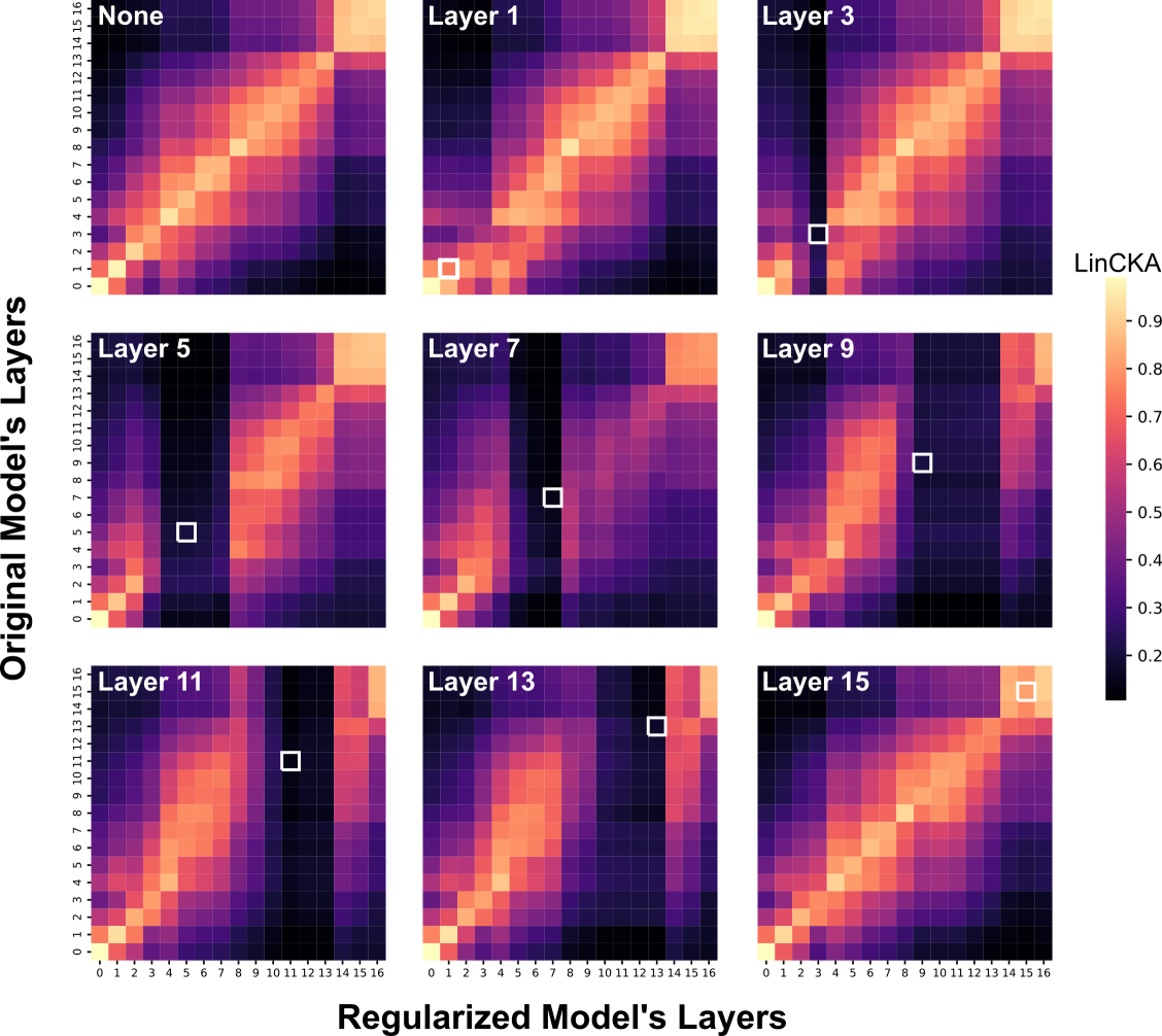
Figure 3: We compare ResNet34s $T$ and $U$ through LinCKA after learning dissimilar representations through ExpVar at a layer of choice. Enforcing representational dissimilarity at different layers leads to highly dissimilar representations between models. Early and later layers remain more similar while intermediate layers can easily be regularized. A visualization of the diagonal LinCKA values can be found in Figure 7.

3.2 Dissimilar representations are unique

Given that independent models converge to very similar solutions, one might assume that models, trained to be dissimilar from them may end up being highly similar to each other. This assumption seems to be amiss, as we observe high representational dissimilarity between the models, see Figure 4. The regularized models are even more dissimilar to each other than they are to the base model they were regularized on, highlighting that the different models learn unique dissimilar solutions to the baseline models.

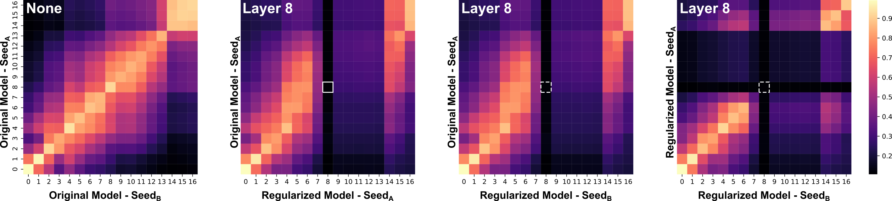
Figure 4: From left to right LinCKA of ResNet34 models regularized with ExpVar: 1) Unregularized models compared to each other. 2) An unregularized model compared to a regularized model from its sequence. 3) An unregularized model compared to a regularized model from a different sequence. 4) A regularized model to another regularized model from a different sequences. Since models from different sequences are not enforced to be dissimilar we denote the layer of regularization as dashed .

3.3 Ensembles of dissimilar models

After establishing that models can learn dissimilar representations we extend the setting to larger number of models training an ensemble of $N=5$ ResNet34s and compare them to each other as visualized in Figure 5. We observe high dissimilarity between early models at the chosen layer, while later models have a less pronounced similarity decrease to existing models. We attribute this to the fact that all representations are merged to approximate the new model, resulting in the new models learning dissimilar representations to this group and not every single model. While this effect looks like efficacy decreases with growing numbers, the model still learns lower similarity levels than the independently trained baseline.

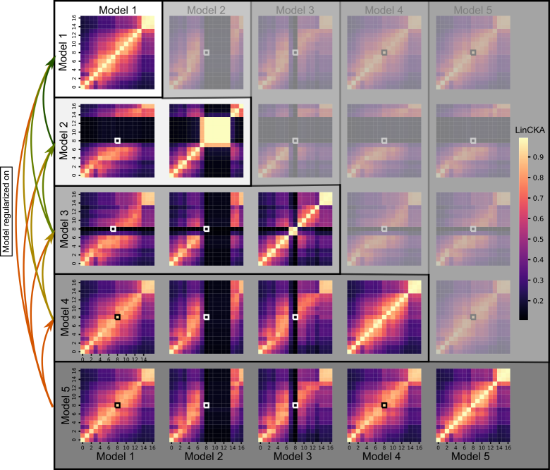
Figure 5: LinCKA between all members of a single ensemble regularized with ExpVar at layer 8. The models are trained sequentially with every new model $U$ being regularized on all existing models.

3.4 Downstream effects of internal dissimilarity

Due to the compositional nature of networks (Eq. 1) we wonder if high internal dissimilarity translates to less correlated predictive behavior between the model pairs. To this end we compare the absolute ensemble performance, the error consistency Cohen’s Kappa $\kappa$ between models (see Section B.2) and the accuracy of the latest trained model $Acc_{U}$ for an ensemble of up to 5 models, see Table 1. We observe that regularizing representational similarity leads to an overall decrease in Cohen’s Kappa of $3\%$ up to $7\%$, while largely maintaining single model performance. Subsequently the ensemble composed of dissimilar models features higher ensemble performance than the baseline ensemble of independently trained models, for every number of models in the ensemble.

Table 1: Ensembles of ResNet34, regularized at various layers with the ExpVar metric. Best metrics are displayed bold, while metrics better than the baseline are underlined.

Output metric	Dissimilarity		Ensemble of N Models
	Metric	Layer	2	3	4	5
Ensemble Acc. [$\%$] $\uparrow$	Baseline	-	95.438 ±0.087	95.730 ±0.082	95.880 ±0.073	95.936 ±0.081
	ExpVar	1	95.580 ±0.189	95.914 ±0.039	96.014 ±0.048	96.130 ±0.042
		3	95.543 ±0.147	95.877 ±0.118	95.968 ±0.112	95.975 ±0.038
		8	95.570 ±0.010	95.897 ±0.006	96.050 ±0.092	96.103 ±0.025
		13	95.748 ±0.114	95.906 ±0.113	95.970 ±0.029	96.034 ±0.076
$Acc_{U}$ [%] $\uparrow$	Baseline	-	94.708 ±0.223	94.828 ±0.165	94.918 ±0.163	94.898 ±0.134
	ExpVar	1	94.426 ±0.292	94.810 ±0.079	94.942 ±0.100	94.896 ±0.302
		3	94.325 ±0.254	94.903 ±0.043	94.875 ±0.186	94.832 ±0.163
		8	94.403 ±0.146	94.733 ±0.377	94.707 ±0.095	94.770 ±0.425
		13	94.608 ±0.304	94.772 ±0.173	94.828 ±0.278	94.636 ±0.204
$\kappa$ [$\%$] $\downarrow$	Baseline	-	52.045 ±0.707	51.852 ±1.417	51.478 ±1.226	51.588 ±1.113
	ExpVar	1	45.636 ±1.696	47.153 ±1.162	48.052 ±0.683	48.377 ±1.035
		3	45.472 ±1.844	46.818 ±0.931	48.125 ±0.498	48.601 ±0.542
		8	45.358 ±0.839	46.438 ±0.801	46.838 ±1.217	46.776 ±1.590
		13	44.361 ±0.803	46.771 ±0.708	48.169 ±0.772	48.692 ±0.327

4 Discussion, Limitations and Conclusion

In this paper we enforce models to learn very dissimilar internal representations to preexisting models by applying various metrics from the field of representational similarity in a novel way. We show that learning features that can’t be approximated through linear regression at an intermediate layer position can result in lower error consistency between the two models. Furthermore we show that this slight decrease in error-consistency suffices to improve overall ensemble accuracy over an ensemble of independent models.

While we show that error consistency between models can be decreased through representational dissimilarity, the decrease is still slight, showing a decrease between 7% to 3% points. Optimally one would like to achieve Cohen’s Kappa scores of $<0$ to maximize ensembling benefits.

Furthermore, we could explore only a small subset of all experiments we deem interesting and have to leave a lot of interesting questions for future work, e.g.: (a) Which features does the dissimilar model learn? (b) Does the dissimilar model end up in a disjoint loss minimum? Can it still be stitched? (c) Which position reduces Cohen’s Kappa the most while maintaining single model performance? (d) Are there other metrics that decrease error consistency more strongly with less effect on accuracy?

Overall, we provide a proof of concept, that enforcing models to learn dissimilar representations also results in different predictive behavior, providing another avenue to make models learn different, novel features, with the goal of achieving robust ensembles.

Appendix A Experiment Details

In this paper the architectures we use are ResNet18s, ResNet34s and ResNet101s trained on CIFAR10 and CIFAR100. Across all experiment settings we train 5 indepedent runs that differ by their random seed, including the ensemble sequence experiments.

A.1 Hyperparameters

All hyperparameters were optimized to maximize single model validation accuracy, as one would in a normal training setting. Finding best performing hyperparameters is a crucial step in order to assure that the developed methodology does not only work for less accurate models where more predictions errors are made and the diversification task becomes easier. We conducted this process for all datasets separately, with all architectures sharing the same final hyperparameter settings.

Once found on single models the hyperparameters were frozen and not adapted to the dissimilarity regularization scheme, avoiding optimizing hyperparameters when starting the dissimilarity regularization experiments. The following hyperparameters for the different architectures were used:

CIFAR10

We train the architectures for $250$ epochs with a batch size of $128$, trained with nesterov SGD, learning rate of $0.1$, momentum $0.9$, cosine annealing learning rate schedule and weight decay $5e-4$. For augmentations we use RandomCrops of size $32\times 32$ with padding $4$, the AutoAugment CIFAR10 policy from Cubuk et al. (2019), followed by Cutout of with size $16$, finished by normalizing the images.

CIFAR100

We utilize the same hyperparameters from CIFAR10 just with a shorter epoch time of $200$.

A.2 Architectures

We train ResNet18, ResNet34 and ResNet101, with the extraction positions being before the $ReLU$ activation function, as highlighted in Figure 6. All ResNets (He et al., 2016) are composed of 4 blocks containing various number of layers per block with a constant amount of channels per block.

ResNet18

Our ResNet18 is composed of four residual blocks of (2-2-2-2) layers with (64-128-256-512) channels each, using basic residual blocks without the inverse bottleneck structure.

ResNet34

ResNet34 is composed of four residual blocks of (3-4-6-3) layers with (64-128-256-512) channels each, using basic residual blocks without inverse bottleneck structure.

ResNet101

ResNet101 is composed of four residual blocks of (3-4-23-3) layers with (256-512-1024-2048) channels respectively, using inverse bottleneck structure of blocks.

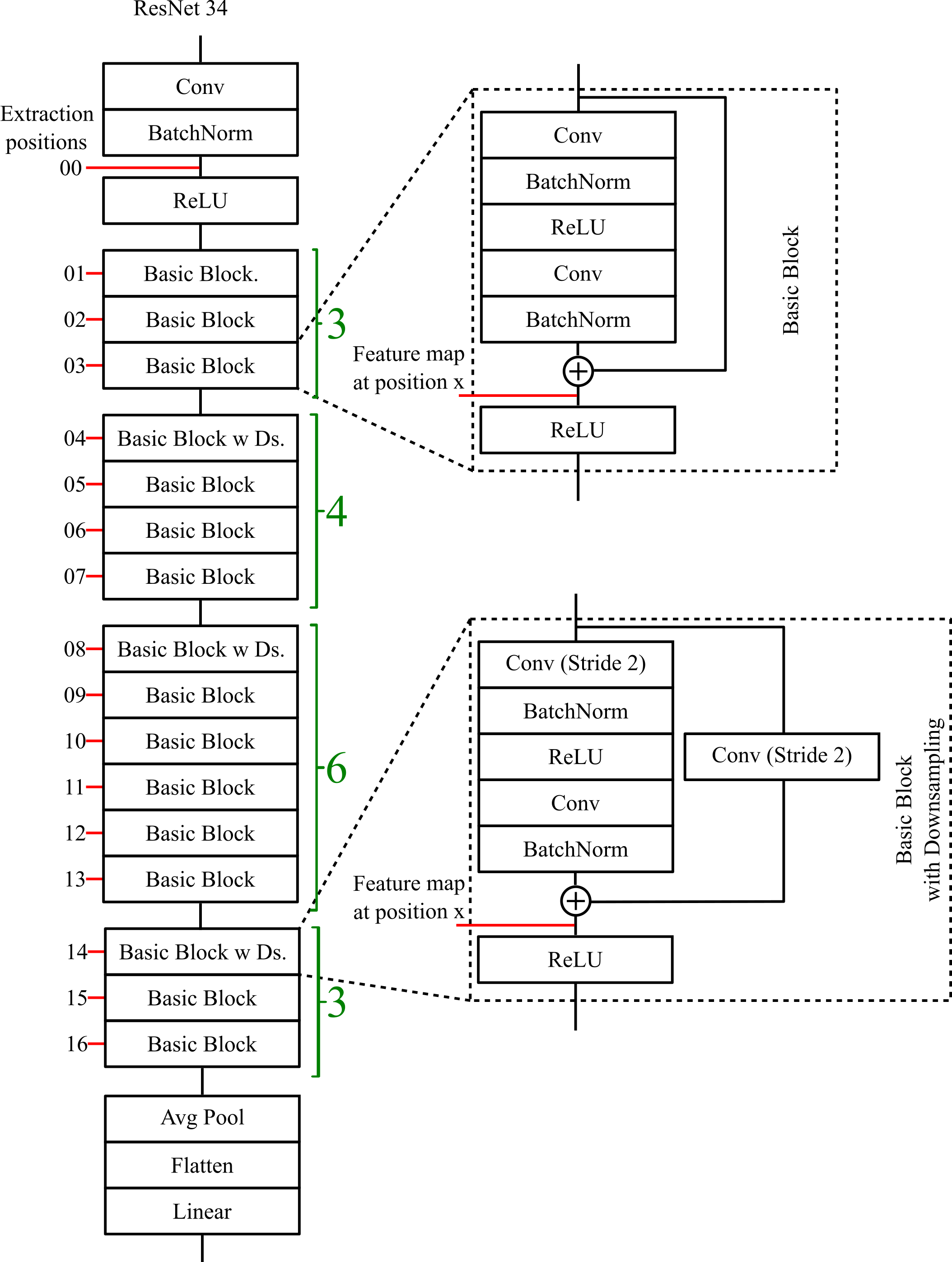
Figure 6: We extract the representations z before the ReLU activation funciton at a location where no skip connection circumvents the current layer. Exemplary ResNet34, using "basic blocks" with or without spatial reduction. We refer to this as ResNet34 with residual blocks of depth (3-4-23-3).

A.3 Evaluation

All results provided in this document are calculated on the test sets of the respective datasets. For CIFAR10 and CIFAR100 we use the official test set of $N=10000$ samples to evaluate both, representational similarity between models and output metrics between models.

For an ensemble $>2$, most of the output metrics like Cohen’s Kappa $\kappa$, $JSD$ and $ERD$ are not directly defined. Hence, we calculate the pairwise metrics and average them over all pairs, leading to an average value which we report in e.g. Table 1.

Appendix B Metrics

The metrics we employ in this study are threefold: L2-Correlation (L2Corr), explained variance (ExpVar) and the sub-space metric Linear Centered Kernel Alignment (LinCKA) (Kornblith et al., 2019) as similarity measures $\mathcal{S}$.

B.1 (Dis)similarity metrics

Aligned metrics

Some metrics compare channels directly and subsequently need exact alignment between the channels of the two networks $U$ and $T$. This channel alignment is non-existent when trained independently and needs to be learned. Hence, we utilize the linear projection to learn channel-wise alignment, as explained in Section 2. We implement this linear projection through a $1\times 1$ Convolution, which maintains spatial information. Given these aligned, approximated values Eq. 4 of the new representation $\textbf{z}_{U}$, we can calculate the L2Corr $r_{c}$ and ExpVar $R^{2}$ for each channel.

$$r_{c}(\textbf{z}_{c},\hat{\textbf{z}}_{c})={\frac{\sum_{i=1}^{n}(\textbf{z}_{i}-{\bar{\textbf{z}}})(\hat{\textbf{z}}_{i}-{\hat{\bar{\textbf{z}}}})}{{\sqrt{\sum_{i=1}^{n}(\textbf{z}_{i}-{\bar{\textbf{z}}})^{2}}}{\sqrt{\sum_{i=1}^{n}(\hat{\textbf{z}}_{i}-{\hat{\bar{\textbf{z}}}})^{2}}}}}$$ (7)

$$R^{2}_{c}(\textbf{z}_{c},\hat{\textbf{z}}_{c})=1-\frac{\sum_{i=1}^{n}(\mathbf{z}_{i}-\mathbf{\hat{\textbf{z}}}_{i})^{2}}{\sum_{i=1}^{n}(\mathbf{z}_{i}-\mathbf{\bar{z}})^{2}}$$ (8)

While the correlation is nicely bounded between $r_{c}\in\{-1,1\}$, the explained variance $R^{2}$ is bounded upwards to 1 but can reach $-\inf$. Therefore we introduce a celu function that wraps the Eq. 8 with $\alpha=1$ that bounds the function.

$$\text{CELU}(R^{2})= \max(0,R^{2})$$ (9)

$$+ \min(0,\alpha\cdot(\exp(R^{2}/\alpha)-1))$$

In the conducted experiments this was necessary to assure stability of the convergence process, as single representation channels $\textbf{z}_{U,c}$ could occasionally feature very low variance close to $0$ in a mini-batch, leading to numeric problems when calculating $R^{2}$ scores.

Given the channel wise scores we average them over all channels resulting in the final score.

$$\text{{ExpVar}}\coloneqq\frac{1}{C}\cdot\sum^{C}_{c=0}\text{CELU}(R^{2}_{c})$$ (10)

$$\text{L2Corr}\coloneqq\frac{1}{C}\cdot\sum^{C}_{c=0}\text{CELU}(r_{c})$$ (11)

Sub-space metrics

Layers of CNNs are composed of multiple channels with the directly following convolution combining the values of its preceding layer through a linear weighted sum of $k\times k\times C$ spanning all channels, making channel order irrelevant and a subject to the stochastic optimization process. This lack of alignment of single neurons was highlighted by (Li et al., 2016) showing that no perfect one-to-one matching of single channels/neurons exists. This insight led to the field of sub-space metrics, which don’t try to measure similarity between single channels/neurons but view the stack of channels as vectors spanning a sub-space (Raghu et al., 2017; Morcos et al., 2018; Wang et al., 2018; Kornblith et al., 2019). These spanned sub-spaces can then be compared directly.

In this paper we use linear Centered Kernel Alignment (CKA) (Kornblith et al., 2019) a metric inspired by the dissimilarity matrices of the neuroscience domain(Kriegeskorte, 2008), which does not need this channel alignment either. Linear Centered Kernel Alignment itself leverages the Hilbert-Schmidt Independence Criterion (HSIC) to compare the similarity of such similarity matrices. In this work we use the unbiased HSIC estimator (Eq. 13) introduced by (Song et al., 2012) and used in mini-batch CKA (Eq. 12) as introduced by (Nguyen et al., 2021).

$$\begin{split}&\text{CKA}_{minibatch}(\textbf{K},\textbf{L})=\\ &\frac{\frac{1}{k}{\sum_{i=1}^{k}}\text{HSIC}(K_{i},L_{i})}{\sqrt{\frac{1}{k}\sum_{i=1}^{k}\text{HSIC}(K_{i},K_{i})}\sqrt{\frac{1}{k}\sum_{i=1}^{k}\text{HSIC}(L_{i},L_{i})}}\end{split}$$ (12)

$$\begin{split}&\text{HSIC}(\textbf{K},\textbf{L})=\frac{1}{n(n-3)}\\ &\cdot\left(tr(\tilde{\textbf{K}}\tilde{\textbf{L}})+\frac{\textbf{1}^{T}\tilde{\textbf{K}}\textbf{1}\textbf{1}^{T}\tilde{\textbf{L}}\textbf{1}}{(n-1)(n-2)}-\frac{2}{n-2}\textbf{1}^{T}\tilde{\textbf{K}}\tilde{\textbf{L}}\textbf{1}\right)\end{split}$$ (13)

B.2 Output prediction metrics

Cohen’s Kappa

Cohen’s Kappa (Cohen, 1960) measures the error consistency between predictors. Specifically it measures the observed error overlap $e_{obs}$ over a cohort $N$ and relates it to the expected error overlap $e_{exp}$ given the accuracies of the predictors while assuming independence between the raters. A $\kappa$ of 0 indicates that the observed error overlap between the two raters is exactly the expected value of error overlap given the two raters accuracies, indicating that the raters are independent. Values of 1 indicate that when one raters errs the other errs as well, whereas negative values indicate that if one rater errs the other is more likely to be correct on the case.

$$\kappa =\frac{e_{obs}-e_{exp}}{1-e_{exp}}$$ (14)

Given an ensemble of models a low or negative value of $\kappa$ is highly desirable as it indicate that the models do not fail on the same samples, leading to high uncertainty on disagreed upon cases or given enough models a correct consensus.

Following up on this error-inconsistency was introduced, which measures when one or the other rater fails but not both. The error-inconsistency is a desirable feature as high values indicate that mistakes are disjoint and, given enough models in an ensemble, can be corrected to improve ensemble performance significantly (Gontijo-Lopes et al., 2022).

Jensen-Shannon Divergence

The Jensen-Shannon divergence (JSD) measures the similarity between two distributions and is based on the Kullbach-Leibeler-Divergence (KL-Divergence) $D$. Opposed to Cohen’s Kappas, which only cares about the argmax prediction being right or wrong, it works with the probability distributions of two models instead, measuring changes in predictive behaviour in a less discrete way.

$$JSD(P\|Q) =\frac{1}{2}\left(D(P\|M)+D(Q\|M)\right)\text{, with}$$ (15)

$$M =\frac{1}{2}(P+Q)$$ (16)

In our case, the probability distribution is represented by the output softmax probabilities of the models, hence the JSD measures how similar the distributions of the two models predictions are before assigning a hard label.

Error disagreement ratio

Additionally to the established metrics, we propose a metric we term error disagreement ratio (EDR), which measures the ratio of different errors to identical errors between two predictors for all joint errors $N_{wrong}$ (Eq. 17). If two models disagree in their errors as often as they agree on their errors EDR is 1. Should the models always agree on their errors the EDR would be 0 and the EDR is greater than 1 for cases where the models disagree more often than agree when both err.

Given that silent failures are detrimental for the applicability of deep learning methods, a high EDR is wanted, yet the EDR in our baselines is commonly $<1$ around $0.3$.

$$\text{EDR}(\hat{p}_{1},\hat{p}_{2})=\frac{\sum^{N_{wrong}}_{i}(1-eq(\hat{p}_{1_{i}},\hat{p}_{2_{i}})}{\sum^{N_{wrong}}_{i}eq(\hat{p}_{1_{i}},\hat{p}_{2_{i}})}$$ (17)

$$\text{eq}(\hat{p}_{1_{i}},\hat{p}_{2_{i}})=\begin{cases}1,&\text{if }\hat{p}_{1_{i}}=\hat{p}_{2_{i}}\\ 0,&\text{else}\\ \end{cases}$$ (18)

Appendix C Dissimilarity ablations

Additionally to the experiments in the main body, we provide additional information and ablations. The additional ablations include the effect of changing the dissimilarity weight $\lambda$ and metric, the number of layers used for regularization and the architectures.

C.1 Layers

Complimentary to Section 3.1, we provide the diagonal LinCKA similarity of the models from Figure 3. When choosing a layer for regularization, the LinCKA similarity decreases the most at the selected layer, mostly affecting layers that are part of its residual block. After a downsampling stage, the similarity tends to increase drastically, but still stays below baseline levels (see Figure 7).

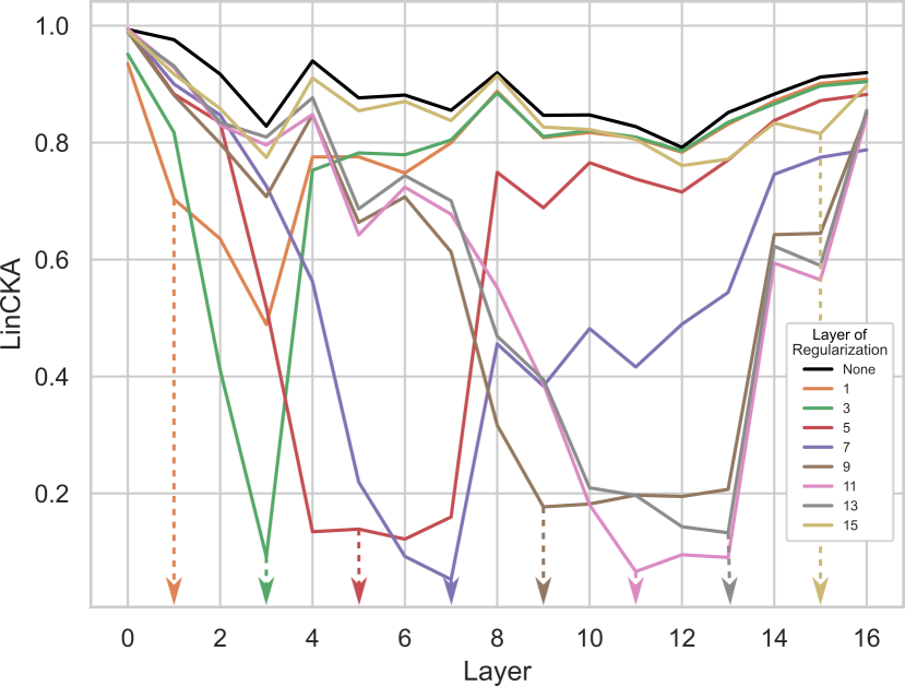
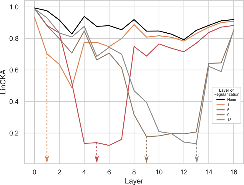
Figure 7: LinCKA between two ResNet34s with the last model being regularized on the former at a specific architecture position. Left: Diagonal LinCKA values of all plots from Figure 3. Right: Diagonal LinCKA values of a smaller subset for better visibility.

C.2 Regularizing multiple layers

Additionally to the previously described setting, one can choose to enforce dissimilarity at multiple layers simultaneously as opposed to only a single selected layer. When choosing multiple layers, the decrease in similarity from baseline is lower than when regularizing only a single layer, as the dissimilarity loss is averaged over all layers. This is highlighted in Figure 8. It nicely portraits the decrease of dissimilarity as more layers are regularized at once.

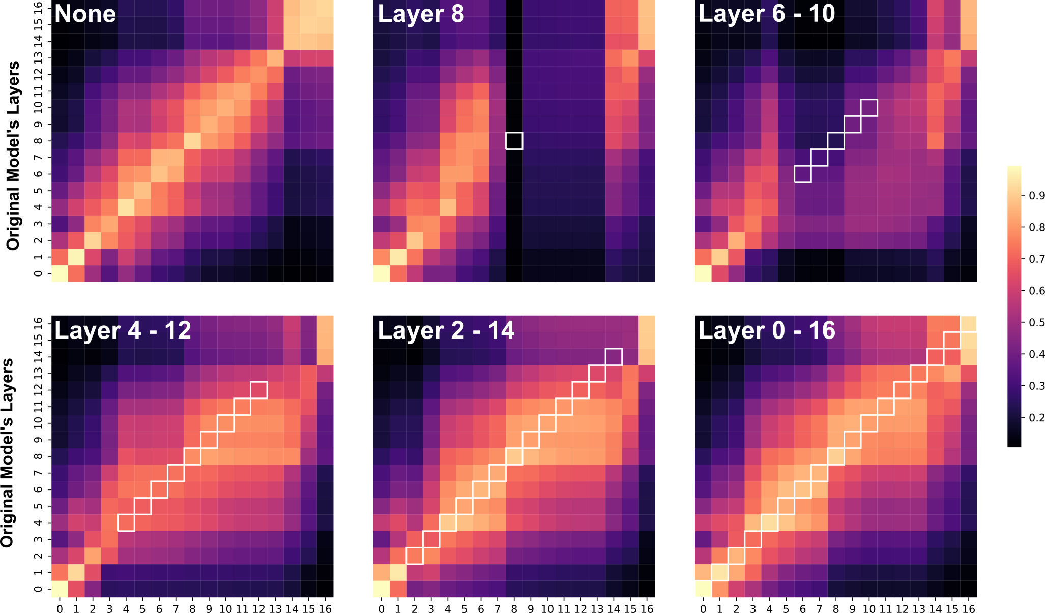
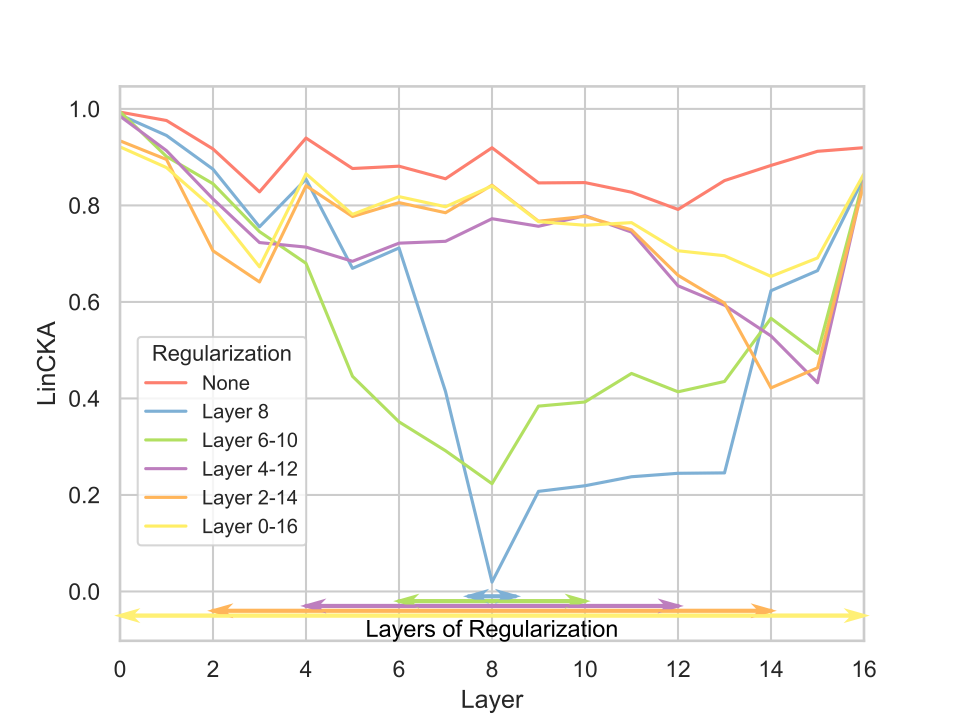
Figure 8: Regularizing at multiple layers leads to decreases in a wider area but to a lower overall decrease than single selected layers.

C.3 ResNet101 and CIFAR100

We expand the experiments to deeper architectures on CIFAR100, as previous experiments were constrained to CIFAR10 and ResNet34.

Layer regularization

Similarly to Section 3.1 we regularize ResNet101 at a very early location Layer $1$, an early layer $3$, a intermediate Layer $20$, and a later layer $32$, visualized in Figure 9. Similarly to the smaller ResNet34 we observe that learned dissimilarity is either localized to the explicit layer of choice or affects the layers of the residual block the regularized layer is situated in. This is especially prominent for the 23 layer deep residual block when regularizing Layer $20$.

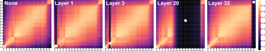
Figure 9: LinCKA values of ResNet101s regularized at different layers by minimizing LinCKA between models on CIFAR100.

C.4 Evaluating different dissimilarity metrics and loss weights

In our experiments we so far constrained ourselves to ExpVar and LinCKA with $\lambda=1$. In order to evaluate if this regularization weight is too strong or too weak, we ablate it for $\lambda\in\{0.25,1.0,4.0\}$ in Table 2 Table 3, and Table 4. Across all metrics one can see that increasing $\lambda$ decreases Cohen’s $\kappa$ and increases $JSD$ while simultaneously decreasing the accuracy of the new model. Setting $\lambda$ too high can lead to instabilities, and significantly reduced ensembling performance as is the case for L2Corr. Furthermore we can observe that different layers require different $\lambda$ values as no one value dominates the others for the entire architecture, complicating the process, should one want to optimize $\lambda$.

Table 2: Output metrics of ResNet34 regularized through ExpVar at various layers.

Metric	Layer	Loss Weight	Ensemble Acc	New Model Acc	Cohens Kappa	JSD	ERD
ExpVar	1	0.25	95.590 ±0.154	94.866 ±0.198	48.006 ±1.237	2.887 ±0.088	33.113 ±3.534%
ExpVar	1	1.00	95.584 ±0.191	94.404 ±0.366	44.961 ±2.389	3.412 ±0.263	36.627 ±5.932%
ExpVar	1	4.00	95.536 ±0.091	93.716 ±1.561	41.594 ±7.017	4.113 ±1.495	46.085 ±11.372%
ExpVar	3	0.25	95.286 ±0.180	94.036 ±0.384	47.923 ±3.376	3.187 ±0.346	35.620 ±5.063%
ExpVar	3	1.00	95.512 ±0.149	94.194 ±0.283	44.867 ±1.541	3.389 ±0.135	40.767 ±5.076%
ExpVar	3	4.00	95.408 ±0.166	94.244 ±0.461	46.050 ±1.636	3.304 ±0.162	37.850 ±2.064%
ExpVar	8	0.25	95.552 ±0.126	94.838 ±0.239	48.798 ±1.321	2.823 ±0.019	35.708 ±2.977%
ExpVar	8	1.00	95.586 ±0.230	94.336 ±0.254	43.303 ±1.521	3.584 ±0.060	42.741 ±3.601%
ExpVar	8	4.00	95.656 ±0.188	94.240 ±0.310	42.671 ±0.769	3.756 ±0.196	38.315 ±2.720%
ExpVar	13	0.25	95.454 ±0.139	94.698 ±0.165	48.873 ±1.717	2.865 ±0.077	32.910 ±0.984%
ExpVar	13	1.00	95.482 ±0.280	93.574 ±1.132	40.243 ±4.897	4.519 ±1.412	43.949 ±7.067%
ExpVar	13	4.00	95.268 ±0.125	93.742 ±0.335	43.711 ±0.620	3.747 ±0.180	40.178 ±3.466%

Table 3: Output metrics of ResNet34 regularized through LinCKA at various layers.

Metric	Layer	Loss Weight	Ensemble Acc [%]	New Model Acc [%]	Cohens Kappa [%]	JSD [%]	ERD [%]
LinCKA	1	0.25	95.656 ±0.143	94.660 ±0.256	47.593 ±.933	3.170 ±0.212	32.005 ±2.659
LinCKA	1	1.00	95.538 ±0.153	94.534 ±0.146	46.511 ±.382	3.336 ±0.391	32.972 ±3.915
LinCKA	1	4.00	95.585 ±0.093	94.450 ±0.261	46.532 ±.352	3.336 ±0.218	32.477 ±5.028
LinCKA	3	0.25	95.536 ±0.194	94.838 ±0.302	51.064 ±.022	2.740 ±0.084	33.170 ±3.865
LinCKA	3	1.00	95.564 ±0.059	94.832 ±0.069	49.281 ±.796	2.858 ±0.173	28.752 ±3.523
LinCKA	3	4.00	95.590 ±0.131	94.852 ±0.084	48.930 ±.531	2.893 ±0.057	35.783 ±3.018
LinCKA	8	0.25	95.520 ±0.172	94.916 ±0.305	49.681 ±.818	2.840 ±0.149	29.145 ±4.743
LinCKA	8	1.00	95.654 ±0.184	94.950 ±0.465	49.399 ±.225	2.843 ±0.203	33.563 ±1.808
LinCKA	8	4.00	95.604 ±0.201	94.816 ±0.234	47.883 ±.204	2.982 ±0.153	34.566 ±4.494
LinCKA	13	0.25	95.512 ±0.115	94.838 ±0.223	51.030 ±.478	2.708 ±0.124	29.956 ±1.436
LinCKA	13	1.00	95.490 ±0.148	94.676 ±0.132	49.758 ±.719	2.832 ±0.125	34.973 ±2.744
LinCKA	13	4.00	95.560 ±0.062	94.720 ±0.190	49.935 ±.917	2.854 ±0.136	33.426 ±4.583

Table 4: Output metrics of ResNet34 regularized through L2Corr at various layers.

Metric	Layer	Loss Weight	Ensemble Acc [%]	New Model Acc [%]	Cohens Kappa [%]	JSD [%]	ERD [%]
L2Corr	1	0.25	94.878 ±0.236	84.932 ±3.072	20.040 ±5.378	12.277 ±3.154	78.008 ±12.239
L2Corr	1	1.00	95.280 ±0.372	70.014 ±24.841	20.176 ±26.374	27.264 ±24.040	125.746 ±91.014
L2Corr	1	4.00	94.770 ±0.138	36.706 ±37.475	1.727 ±9.740	51.226 ±28.757	358.925 ±221.863
L2Corr	3	0.25	95.580 ±0.306	94.492 ±0.811	46.383 ±3.550	3.291 ±0.675	35.765 ±8.759
L2Corr	3	1.00	95.636 ±0.131	94.660 ±0.453	46.918 ±1.769	3.205 ±0.337	34.598 ±5.420
L2Corr	3	4.00	95.346 ±0.595	75.138 ±37.168	31.375 ±24.993	19.251 ±29.950	133.428 ±197.775
L2Corr	8	0.25	95.652 ±0.088	94.920 ±0.135	48.895 ±2.401	2.877 ±0.098	36.460 ±3.253
L2Corr	8	1.00	95.638 ±0.173	94.864 ±0.192	47.767 ±1.476	2.976 ±0.119	33.190 ±2.801
L2Corr	8	4.00	95.684 ±0.142	94.854 ±0.157	48.318 ±2.705	3.015 ±0.145	32.675 ±4.037
L2Corr	13	0.25	95.532 ±0.163	94.718 ±0.175	50.558 ±1.417	2.768 ±0.080	33.224 ±2.386
L2Corr	13	1.00	95.512 ±0.155	94.684 ±0.312	49.418 ±0.510	2.829 ±0.081	37.031 ±3.395
L2Corr	13	4.00	95.322 ±0.094	93.846 ±0.281	47.663 ±1.640	3.329 ±0.180	39.130 ±4.778

C.5 More detailed output metrics

Revisiting Eq. 5 the factor lambda determines the importance of learning representations that are dissimilar. Given that we observe Table 1 in the main did not contain all metrics of interest we gathered, hence we provide the table containing additional metrics like the Jensen-Shannon-Divergence (JSD) (see Section B.2).

Table 5: Ensembles of ResNet34, regularized at various layers with the ExpVar metric. Best metrics are displayed bold, while metrics better than the baseline are underlined.

Output metric	Dissimilarity		Ensemble of N Models
	Metric	Layer	2	3	4	5
Ensemble Acc. [$\%$] $\uparrow$	Baseline	-	95.438 ±0.087	95.730 ±0.082	95.880 ±0.073	95.936 ±0.081
	ExpVar	1	95.580 ±0.189	95.914 ±0.039	96.014 ±0.048	96.130 ±0.042
		3	95.543 ±0.147	95.877 ±0.118	95.968 ±0.112	95.975 ±0.038
		8	95.570 ±0.010	95.897 ±0.006	96.050 ±0.092	96.103 ±0.025
		13	95.748 ±0.114	95.906 ±0.113	95.970 ±0.029	96.034 ±0.076
$Acc_{U}$ [$\%$] $\uparrow$	Baseline	-	94.708 ±0.223	94.828 ±0.165	94.918 ±0.163	94.898 ±0.134
	ExpVar	1	94.426 ±0.292	94.810 ±0.079	94.942 ±0.100	94.896 ±0.302
		3	94.325 ±0.254	94.903 ±0.043	94.875 ±0.186	94.832 ±0.163
		8	94.403 ±0.146	94.733 ±0.377	94.707 ±0.095	94.770 ±0.425
		13	94.608 ±0.304	94.772 ±0.173	94.828 ±0.278	94.636 ±0.204
$\kappa$ [$\%$] $\downarrow$	Baseline	-	52.045 ±0.707	51.852 ±1.417	51.478 ±1.226	51.588 ±1.113
	ExpVar	1	45.636 ±1.696	47.153 ±1.162	48.052 ±0.683	48.377 ±1.035
		3	45.472 ±1.844	46.818 ±0.931	48.125 ±0.498	48.601 ±0.542
		8	45.358 ±0.839	46.438 ±0.801	46.838 ±1.217	46.776 ±1.590
		13	44.361 ±0.803	46.771 ±0.708	48.169 ±0.772	48.692 ±0.327
JSD [$\%$] $\uparrow$	Baseline	-	2.688 ±0.037	2.698 ±0.038	2.692 ±0.014	2.672 ±0.026
	ExpVar	1	3.268 ±0.113	3.146 ±0.153	3.030 ±0.087	2.992 ±0.106
		3	3.386 ±0.227	3.160 ±0.157	3.036 ±0.113	2.978 ±0.096
		8	3.501 ±0.155	3.290 ±0.183	3.204 ±0.207	3.164 ±0.270
		13	3.500 ±0.141	3.253 ±0.104	3.115 ±0.088	3.034 ±0.080
EDR [$\%$] $\uparrow$	Baseline	-	31.596 ±4.426	31.117 ±2.883	30.907 ±0.827	31.154 ±1.536
	ExpVar	1	36.085 ±4.440	34.867 ±2.334	34.105 ±0.374	33.454 ±1.368
		3	37.314 ±3.921	36.548 ±1.820	34.816 ±1.918	34.583 ±1.803
		8	37.817 ±1.288	35.971 ±0.716	34.529 ±0.765	34.157 ±1.554
		13	34.944 ±5.814	33.559 ±2.560	33.154 ±2.072	32.831 ±1.691

Appendix D Choice of similarity metrics

Many elaborate similarity metrics exist, from SVCCA (Raghu et al., 2017) to PWCCA (Morcos et al., 2018) to CKA (Kornblith et al., 2019) a variety of methods can be employed to learn dissimilar representation as all are differentiable.

In this work we decided to keep the metric choice as simple as possible and use aligned regression and correlation metrics ExpVar and L2Corr as their channel-wise nature and alignment allows good interpretability and introspection possibilities for early development. Additionally we included LinCKA as it is the most recent popular similarity metric and has a lower memory footprint than SVCCA, due to it working on the similarity matrices instead of representations directly. Additionally LinCKA can be nicely calculated on mini-batches (Nguyen et al., 2021).

References

- Ainsworth et al. (2023) Ainsworth, S., Hayase, J., and Srinivasa, S. Git re-basin: Merging models modulo permutation symmetries. In The Eleventh International Conference on Learning Representations, 2023. URL https://openreview.net/forum?id=CQsmMYmlP5T.
- Bansal et al. (2021) Bansal, Y., Nakkiran, P., and Barak, B. Revisiting model stitching to compare neural representations. In Beygelzimer, A., Dauphin, Y., Liang, P., and Vaughan, J. W. (eds.), Advances in Neural Information Processing Systems, 2021. URL https://openreview.net/forum?id=ak06J5jNR4.
- Cohen (1960) Cohen, J. A Coefficient of Agreement for Nominal Scales. Educational and Psychological Measurement, 20(1):37–46, 1960. doi: 10.1177/001316446002000104. URL https://doi.org/10.1177/001316446002000104.
- Csiszárik et al. (2021) Csiszárik, A., Kőrösi-Szabó, P., Matszangosz, Á. K., Papp, G., and Varga, D. Similarity and matching of neural network representations. In Beygelzimer, A., Dauphin, Y., Liang, P., and Vaughan, J. W. (eds.), Advances in Neural Information Processing Systems, 2021. URL https://openreview.net/forum?id=aedFIIRRfXr.
- Cubuk et al. (2019) Cubuk, E. D., Zoph, B., Mané, D., Vasudevan, V., and Le, Q. V. Autoaugment: Learning augmentation strategies from data. In 2019 IEEE/CVF Conference on Computer Vision and Pattern Recognition (CVPR), pp. 113–123, 2019. doi: 10.1109/CVPR.2019.00020.
- Dietterich (2000) Dietterich, T. G. Ensemble methods in machine learning. In Lecture Notes in Computer Science (including subseries Lecture Notes in Artificial Intelligence and Lecture Notes in Bioinformatics), volume 1857 LNCS, pp. 1–15. Springer Verlag, 2000. ISBN 3540677046. doi: 10.1007/3-540-45014-9_1. URL https://link.springer.com/chapter/10.1007/3-540-45014-9_1.
- Geirhos et al. (2020) Geirhos, R., Jacobsen, J.-H., Michaelis, C., Zemel, R., Brendel, W., Bethge, M., and Wichmann, F. A. Shortcut learning in deep neural networks. Nature Machine Intelligence, 2:665–673, 2020. URL http://arxiv.org/abs/2004.07780.
- Gontijo-Lopes et al. (2022) Gontijo-Lopes, R., Dauphin, Y., and Cubuk, E. D. No one representation to rule them all: Overlapping features of training methods. In International Conference on Learning Representations, 2022. URL https://openreview.net/forum?id=BK-4qbGgIE3.
- He et al. (2016) He, K., Zhang, X., Ren, S., and Sun, J. Deep residual learning for image recognition. In Proceedings of the IEEE Computer Society Conference on Computer Vision and Pattern Recognition, volume 2016-Decem, pp. 770–778. IEEE Computer Society, dec 2016. ISBN 9781467388504. doi: 10.1109/CVPR.2016.90. URL http://image-net.org/challenges/LSVRC/2015/.
- Islam et al. (2003) Islam, M. M., Yao, X., and Murase, K. A constructive algorithm for training cooperative neural network ensembles. IEEE Transactions on Neural Networks, 14(4):820–834, 2003. ISSN 10459227. doi: 10.1109/TNN.2003.813832. URL https://pubmed.ncbi.nlm.nih.gov/18238062/.
- Klabunde et al. (2023) Klabunde, M., Schumacher, T., Strohmaier, M., and Lemmerich, F. Similarity of neural network models: A survey of functional and representational measures, 2023.
- Kornblith et al. (2019) Kornblith, S., Norouzi, M., Lee, H., and Hinton, G. Similarity of neural network representations revisited. In 36th International Conference on Machine Learning, ICML 2019, volume 2019-June, pp. 6156–6175, 2019. ISBN 9781510886988. URL https://arxiv.org/abs/1905.00414.
- Kriegeskorte (2008) Kriegeskorte, N. Representational similarity analysis – connecting the branches of systems neuroscience. Frontiers in Systems Neuroscience, 2:4, 11 2008. ISSN 16625137. doi: 10.3389/neuro.06.004.2008. URL http://journal.frontiersin.org/article/10.3389/neuro.06.004.2008/abstract.
- Lakshminarayanan et al. (2016) Lakshminarayanan, B., Pritzel, A., and Blundell, C. Simple and Scalable Predictive Uncertainty Estimation using Deep Ensembles. Advances in Neural Information Processing Systems, 2017-Decem:6403–6414, dec 2016. URL http://arxiv.org/abs/1612.01474.
- Lenc & Vedaldi (2015) Lenc, K. and Vedaldi, A. Understanding image representations by measuring their equivariance and equivalence. In 2015 IEEE Conference on Computer Vision and Pattern Recognition (CVPR), pp. 991–999, 2015. doi: 10.1109/CVPR.2015.7298701.
- Li et al. (2016) Li, Y., Yosinski, J., Clune, J., Lipson, H., and Hopcroft, J. Convergent learning: Do different neural networks learn the same representations? In International Conference on Learning Representations, volume 44, pp. 196–212, 2016. URL http://proceedings.mlr.press/v44/li15convergent.pdf.
- Liu & Yao (1999a) Liu, Y. and Yao, X. Ensemble learning via negative correlation. Neural Networks, 12(10):1399–1404, dec 1999a. ISSN 08936080. doi: 10.1016/S0893-6080(99)00073-8.
- Liu & Yao (1999b) Liu, Y. and Yao, X. Simultaneous training of negatively correlated neural networks in an ensemble. IEEE Transactions on Systems, Man, and Cybernetics, Part B: Cybernetics, 29(6):716–725, 1999b. ISSN 10834419. doi: 10.1109/3477.809027.
- Minderer et al. (2020) Minderer, M., Bachem, O., Houlsby, N., and Tschannen, M. Automatic shortcut removal for self-supervised representation learning. In International Conference on Machine Learning, 2020.
- Morcos et al. (2018) Morcos, A. S., Raghu, M., and Bengio, S. Insights on representational similarity in neural networks with canonical correlation. Advances in Neural Information Processing Systems, 2018-Decem:5727–5736, jun 2018. URL http://arxiv.org/abs/1806.05759.
- Moschella et al. (2023) Moschella, L., Maiorca, V., Fumero, M., Norelli, A., Locatello, F., and Rodolà, E. Relative representations enable zero-shot latent space communication. In The Eleventh International Conference on Learning Representations, 2023. URL https://openreview.net/forum?id=SrC-nwieGJ.
- Nguyen et al. (2021) Nguyen, T., Raghu, M., and Kornblith, S. Do wide and deep networks learn the same things? uncovering how neural network representations vary with width and depth. In International Conference on Learning Representations, 2021. URL https://openreview.net/forum?id=KJNcAkY8tY4.
- Pang et al. (2019) Pang, T., Xu, K., Du, C., Chen, N., and Zhu, J. Improving adversarial robustness via promoting ensemble diversity. In International Conference on Machine Learning, pp. 4970–4979. PMLR, 2019.
- Raghu et al. (2017) Raghu, M., Gilmer, J., Yosinski, J., and Sohl-Dickstein, J. SVCCA: Singular Vector Canonical Correlation Analysis for Deep Learning Dynamics and Interpretability. Advances in Neural Information Processing Systems, 2017-Decem:6077–6086, jun 2017. URL http://arxiv.org/abs/1706.05806.
- Song et al. (2012) Song, L., Smola, A., Gretton, A., Bedo, J., and Borgwardt, K. Feature selection via dependence maximization. Journal of Machine Learning Research, 13:1393–1434, 2012. ISSN 15324435.
- Theisen et al. (2023) Theisen, R., Kim, H., Yang, Y., Hodgkinson, L., and Mahoney, M. W. When are ensembles really effective?, 2023.
- Wang et al. (2018) Wang, L., Hu, L., Gu, J., Hu, Z., Wu, Y., He, K., and Hopcroft, J. Towards understanding learning representations: To what extent do different neural networks learn the same representation. Advances in neural information processing systems, 31, 2018.