Wasserstein Auto-Encoders of Merge Trees
(and Persistence Diagrams)

Abstract

This paper presents a computational framework for the Wasserstein auto-encoding of merge trees (MT-WAE), a novel extension of the classical auto-encoder neural network architecture to the Wasserstein metric space of merge trees. In contrast to traditional auto-encoders which operate on vectorized data, our formulation explicitly manipulates merge trees on their associated metric space at each layer of the network, resulting in superior accuracy and interpretability. Our novel neural network approach can be interpreted as a non-linear generalization of previous linear attempts at merge tree encoding. It also trivially extends to persistence diagrams. Extensive experiments on public ensembles demonstrate the efficiency of our algorithms, with MT-WAE computations in the orders of minutes on average. We show the utility of our contributions in two typical applications of auto-encoders. First, we apply MT-WAE to data reduction and reliably compress merge trees by concisely representing them with their coordinates in the final layer of our auto-encoder. Second, we present a dimensionality reduction framework exploiting the latent space of our auto-encoder, for the visual analysis of ensemble data. We illustrate the versatility of our framework by introducing two penalty terms, to help preserve in the latent space both the Wasserstein distances between merge trees, as well as their clusters. In both applications, quantitative experiments assess the relevance of our framework. Finally, we provide a C++ implementation that can be used for reproducibility.

Visual analysis of the Earthquake ensemble $\big{(}(a)$ one member per ground-truth class$\big{)}$, with our Wasserstein Auto-Encoder of Merge Trees (MT-WAE). We apply our contributions to data reduction, where the input trees can be efficiently compressed $\big{(}(b)$, right$\big{)}$ by simply storing their coordinates in the last decoding layer of our network. We exploit the latent space of our network to generate 2D layouts of the ensemble $(c)$. In contrast to classical auto-encoders, MT-WAE maintains merge trees at each layer of the network, which results in improved accuracy and interpretability. Specifically, the reconstruction of user-defined locations $\big{(}(c)$, purple$)$ enables an interactive exploration of the latent space: the reconstructed curve $(d)$ enables the navigation from the trees of the first cluster $\big{(}$dark red, $(c)\big{)}$, to the second $\big{(}$pink, $(c)\big{)}$ and third $\big{(}$light pink, $(c)\big{)}$ clusters. MT-WAE also supports persistence correlation views $(e)$, which reveal the barycenter’s features which are the most responsible for the variability in the ensemble (far from the center). Finally, by tracking the persistence evolution of individual features as they traverse the network down to its latent space, we introduce a Feature Latent Importance measure, which enables the identification of the most informative features within the ensemble $\big{(}(e)$, red circles$)$.

Introduction

1 Introduction

Figure 1: Visual analysis of the Earthquake ensemble $\big{(}(a)$ each ground-truth class is represented by one of its members$\big{)}$, with our Wasserstein Auto-Encoder of Merge Trees (MT-WAE). We apply our contributions to merge tree compression $\big{(}(b)$, right$\big{)}$ by simply storing their coordinates in the last decoding layer of our network. We exploit the latent space of our network to generate 2D layouts of the ensemble $(c)$. In contrast to classical auto-encoders, MT-WAE explicitly manipulates merge trees at each layer of the network, which results in improved accuracy and interpretability. Specifically, the reconstruction of user-defined locations $\big{(}(c)$, purple$)$ enables an interactive exploration of the latent space: the reconstructed curve $(d)$ enables a continuous navigation between the clusters $\big{(}$from dark red to pink and light pink, $(c)\big{)}$. MT-WAE also supports persistence correlation views $(e)$ (adapted from [pont_tvcg23]), which reveal the barycenter’s persistent features which exhibit the most variability in the ensemble (far from the center). Finally, by tracking the persistence evolution of individual features as they traverse the network down to its latent space, we introduce a Feature Latent Importance measure, which identifies the most informative features within the ensemble $\big{(}(e)$, red circles$)$.

With the recent advances in the development of computation hardware and acquisition devices, datasets are constantly increasing in size. This size increase induces an increase in the geometrical complexity of the features present in the datasets, which challenges interactive data analysis and interpretation. To address this issue, Topological Data Analysis (TDA) [edelsbrunner09] has shown over the years its ability to reveal, in a generic, robust and efficient manner, the main structural patterns hidden in complex datasets, in particular for visual data analysis tasks [heine16]. Successful applications have been documented in multiple fields (turbulent combustion [bremer_tvcg11, gyulassy_ev14], material sciences [gyulassy_vis15, soler_ldav19], nuclear energy [beiNuclear16], fluid dynamics [kasten_tvcg11, nauleau_ldav22], bioimaging [topoAngler, beiBrain18], quantum chemistry [Malgorzata19, olejniczak_pccp23] or astrophysics [sousbie11, shivashankar2016felix]). Among the representations studied in TDA, the merge tree [carr00] (Fig. 2) has been prominent in data visualization [carr04, bremer_tvcg11, topoAngler].

In addition to the increase in geometrical complexity discussed above, a new challenge has recently emerged in many applications, with the notion of ensemble datasets. Such datasets encode a given phenomenon not only with a single dataset, but with a collection of datasets, called ensemble members. In that context, the topological analysis of an ensemble dataset consequently yields an ensemble of corresponding topological representations (e.g. one merge tree per ensemble member).

Then, developing statistical analysis tools to support the interactive analysis and interpretation of ensemble data becomes an important challenge. Recently, several works explored this direction, in particular with the notion of average topological representation [Turner2014, lacombe2018, vidal_vis19, YanWMGW20, pont_vis21]. These approaches can produce a topological representation which nicely summarizes the ensemble. Moreover, their application to clustering [pont_vis21] reveal its main trends. However, they do not provide any hints regarding the variability of the features in the ensemble. For this, Pont et al. [pont_tvcg23] recently extended the notion of principal geodesic analysis to ensembles of merge trees. However, this approach implicitly assumes a linear relation between the merge trees of the ensemble. Specifically, it assumes that merge tree branches evolve linearly (in the birth/death space, Sec. 2) within the ensemble.

This paper addresses this issue with a novel formulation based on neural networks and introduces the first framework for the non-linear encoding of merge trees, hence resulting in superior accuracy. Specifically, we formulate merge tree non-linear encoding as an auto-encoding problem (Sec. 3). We contribute a novel neural network called Wasserstein Auto-Encoder of Merge Trees. This network is based on a novel layer model, capable of processing merge trees natively, without pre-vectorization. We believe this contribution to be of independent interest, as it enables an accurate and interpretable processing of merge trees by neural networks (without restrictions to auto-encoders). We contribute an algorithm for the optimization of such a network (Sec. 4). We illustrate the relevance of our contributions for visual analysis with two applications, data reduction (Sec. 5.1) and dimensionality reduction (Sec. 5.2). Similarly to previous linear attempts [pont_tvcg23], since our approach is based on the Wasserstein distance between merge trees [pont_vis21], which generalizes the Wasserstein distance between persistence diagrams [edelsbrunner09], our framework trivially extends to persistence diagrams by simply adjusting a single parameter.

1.1 Related work

We classify the literature related to our approach into two categories: ensemble analysis and topological methods for ensembles.

(1) Ensemble analysis: Typical approaches to ensemble visualization first characterize each member of the ensemble by extracting a geometrical object representing its features of interest (level sets, streamlines, etc). Next, a second step considers the ensemble of geometrical objects computed in the first step, and estimates a single representative object, representing an aggregate of the features of interest found in the ensemble. For example, level-set variability has been studied with spaghetti plots [spaghettiPlot], with specific applications to weather data [Potter2009, Sanyal2010]. More generally, the variability in curves and contours have been studied with the notion of box-plots [whitaker2013] and its variants [Mirzargar2014]. Hummel et al. [Hummel2013] analyzed the variability in ensembles of flows with a Lagrangian approach. The main trends present in an ensemble have been studied for ensembles of streamlines [Ferstl2016] and level sets [Ferstl2016b] via clustering techniques. Other approaches focused on visualizing the geometrical variability in the domain of the position of critical points [gunther, favelier_vis18] or gradient separatrices [athawale_tvcg19]. For ensemble of contour trees, consistent planar layouts have also been studied [LohfinkWLWG20], to support the direct visual comparison of the trees. While the latter approaches have a topological aspect, they focused on the direct visualization of the variability, and not on the statistical analysis of an ensemble of topological descriptors.

General purpose methods have been documented for non-linear encoding (e.g. topological auto-encoders [MoorHRB20], or Wasserstein auto-encoders [TolstikhinBGS18]). Our work drastically differs from these methods, in terms of design and purpose. These methods [MoorHRB20, TolstikhinBGS18, HenselMR21] employ a classical auto-encoder (Sec. 3.1) to which they add specialized penalty terms. Then, their input is restricted to point sets (or vectorized data). In contrast, our work focuses on sets of merge trees (or persistence diagrams). This different kind of input requires a novel neural network model, capable of processing these topological objects natively (Sec. 3).

(2) Topological methods: Over the last two decades, the visualization community has investigated, adapted and extended [heine16, surveyComparison2021] several tools and notions from computational topology [edelsbrunner09]. The persistence diagram [edelsbrunner02, edelsbrunner09, dipha, guillou_tvcg23], the Reeb graph [biasotti08, parsa12, gueunet_egpgv19], the merge (Fig. 2) and contour trees [carr00, MaadasamyDN12, AcharyaN15, CarrWSA16, gueunet_tpds19], and the Morse-Smale complex [BremerEHP03, Defl15, robins_pami11, ShivashankarN12, gyulassy_vis18] are popular examples of topological representations in visualization.

In order to design a statistical framework for the analysis of ensembles of topological descriptors, one first needs to define a metric to measure distances between these objects. The Wasserstein distance [edelsbrunner09] (Sec. 2.2) is now an established and well-documented metric for persistence diagrams. It is inspired by optimal transport [Kantorovich, monge81] and it is defined (Sec. 2.2) via a bipartite assignment problem (open-source software implementing exact computations [Munkres1957] or fast approximations [Bertsekas81, Kerber2016] is available [ttk17]). However, as discussed in previous work [morozov14, BeketayevYMWH14, SridharamurthyM20, pont_vis21, pont_tvcg23], the persistence diagram can lack specificity in its encoding of the features of interest, motivating more advanced descriptors, like the merge trees (Sec. 2.1), which better distinguishes datasets. The comparison of Reeb graphs and their variants has been addressed with several similarity measures [HilagaSKK01, SaikiaSW14_branch_decomposition_comparison]. Several works investigated the theoretical aspects of distances between topological descriptors, in particular with a focus towards stable distances [bauer14, morozov14, bollen21, BollenTL23]. However, the computation of such distances rely on algorithms with exponential time complexity, which is not practicable for real-life datasets. In contrast, a distinct line of research focused on a balance between practical stability and computability, by focusing on polynomial time computation algorithms. Beketayev et al. [BeketayevYMWH14] introduced a distance for the branch decomposition tree (BDT, Appendix A). Efficient algorithms for constrained edit distances [zhang96] have been specialized to the specific case of merge trees, hence providing an edit distance for merge trees [SridharamurthyM20] which is both computable in practice and with acceptable practical stability. Pont et al. [pont_vis21] extended this work to generalize the $L_{2}$-Wasserstein distance between persistence diagrams [edelsbrunner09] to merge trees, hence enabling the efficient computation of distances, geodesics and barycenters of merge trees. Wetzel et al. [WetzelsLG22, WetzelsTopoInVis22] introduce metrics independent of a particular branch decomposition, but this comes at the cost of a significantly larger computational effort (with quartic time complexity instead of quadratic), which prevents their practical computation on full-sized merge trees.

Once a metric is available, statistical notions can be developed for topological descriptors. Several methods [Turner2014, lacombe2018, vidal_vis19] have been introduced for the estimation of barycenters of persistence diagrams (or vectorized variants [Adams2015, Bubenik15]). Similar approaches have been specifically derived for the merge trees [YanWMGW20, pont_vis21]. Another set of approaches [robins16, AnirudhVRT16, LI2021] first considers vectorizations of topological descriptors (i.e. by converting them into high-dimensional Euclidean vectors) and then leverages traditional linear-algebra tools on these vectors (e.g. the classical PCA [pearson01] or its variants from matrix sketching [woodRuff2014]). Several approaches in machine learning are constructed on top of vectorizations of topological descriptors [Adams2015, Bubenik15, kim20] or kernel-based representations [ReininghausHBK15, CarriereCO17]. However, such vectorizations have several limitations in practice. First, they are prone to approximation errors (resulting from quantization and linearization). Also, they can be difficult to revert (especially for barycenters), which makes them impractical for visualization tasks. Moreover, their stability is not always guaranteed. In contrast, Pont et al. [pont_tvcg23] extended the generic notion of principal geodesic analysis to the Wasserstein metric space of merge trees, resulting in improved accuracy and interpretability with regard to the straightforward application of PCA on merge tree vectorizations. Similarly, Sisouk et al. [sisouk_techrep23] introduced a simpler approach for the linear encoding of persistence diagrams, with a less constrained framework based on dictionaries. However, these approaches implicitly assume a linear relation between the topological descriptors of the ensemble. For instance, it assumes that a given feature (i.e. a given branch of the merge tree) evolves linearly in the birth/death space (Sec. 2) within the ensemble. However, this hypothesis is easily challenged in practice (Figs. 5 and 7), potentially leading to inaccuracies. Our work overcomes this limitation with a drastically different formulation (based on auto-encoding neural networks) and introduces the first framework for the non-linear encoding of merge trees, resulting in superior accuracy. Several approaches [khrulkov18, Gabrielsson19, zhou2021] investigated the use of topological methods for the analysis of neural networks. In contrast, our work targets a different research problem, specifically the encoding of topological descriptors with neural networks.

1.2 Contributions

This paper makes the following new contributions:

1. An approach to Merge tree non-linear encoding: We formulate the non-linear parametrization of the Wasserstein metric space of merge trees (and persistence diagrams) as an auto-encoding problem. Our formulation (Sec. 3) generalizes and improves previous linear attempts [pont_tvcg23].

2. A vectorization-free neural network architecture for Merge Trees: We contribute a novel neural network architecture called Wasserstein Auto-Encoder of Merge Trees, inspired by the classical auto-encoder, which can natively process merge trees (and persistence diagrams) without prior vectorization. For this, we contribute a novel layer model, which takes a set of merge trees on its input and produces another set of merge trees on its output, along with their coordinates in the layer’s parametrization. This results in superior accuracy (Sec. 6.2) and interpretability (Sec. 5.2). We contribute an algorithm for the optimization of this network (Sec. 4). We believe this contribution to be of independent interest.

3. An application to merge tree compression: We describe how to adapt previous work [pont_tvcg23] to our novel non-linear framework, in merge tree compression applications (Sec. 5.1). Specifically, the merge trees of the input ensemble are significantly compressed, by solely storing the final decoding layer of the network, as well as the coordinates of the input trees in this layer. We illustrate the interest of our approach with comparisons to linear encoding [pont_tvcg23] in the context of feature tracking and ensemble clustering applications.

4. An application to dimensionality reduction: We describe how to adapt previous work [pont_tvcg23] to our novel non-linear framework, in the context of dimensionality reduction applications (Sec. 5.2). Specifically, each tree of the ensemble is embedded as a point in a planar view, based on its coordinates in our auto-encoder’s latent space. To illustrate the versatility of our framework, we introduce two penalty terms, to improve the preservation of clusters and distances between merge trees.

5. Implementation: We provide a C++ implementation of our algorithms that can be used for reproducibility purposes.

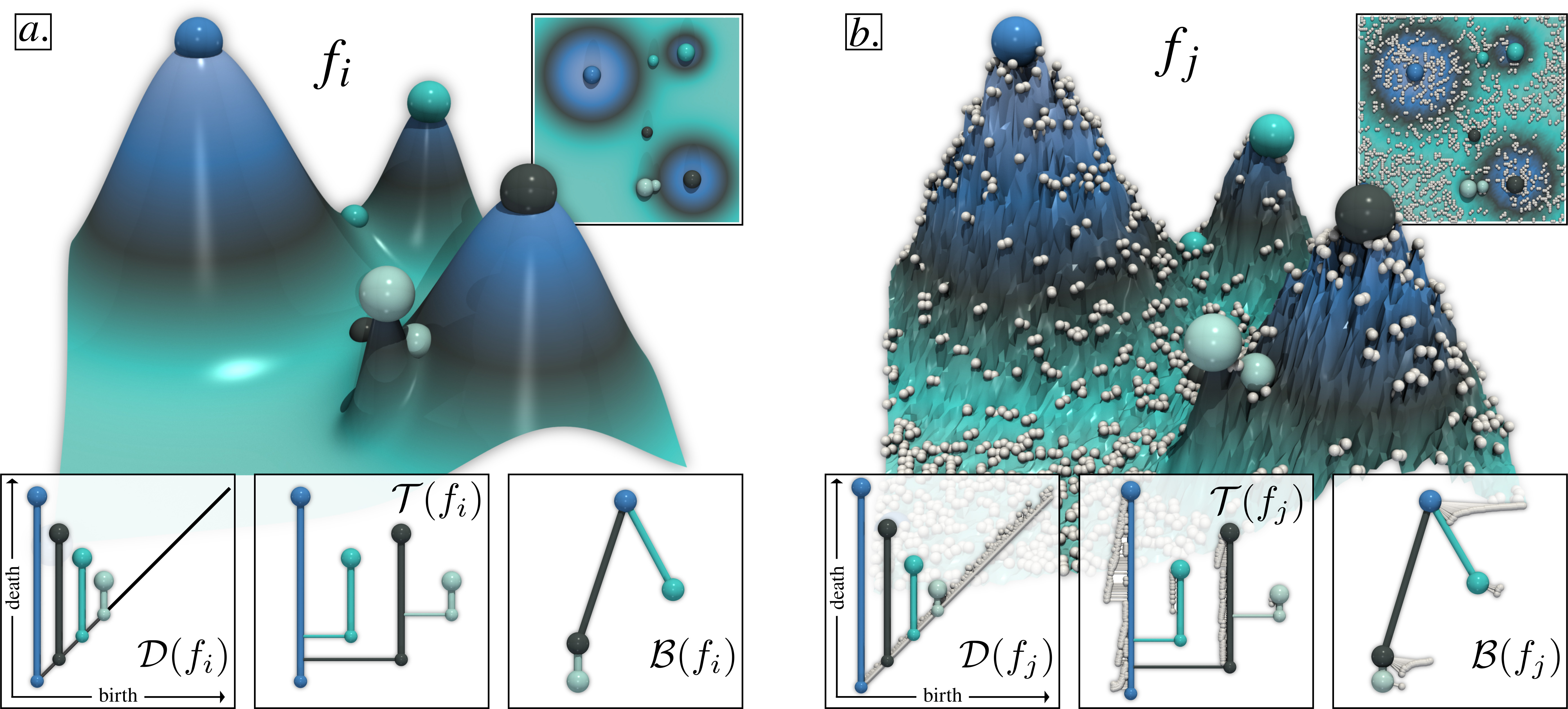
Figure 2: Illustration of the topological descriptors considered in this work, on a clean $(a)$ and a noisy $(b)$ variant of a 2D toy dataset. For all descriptors, the color code indicates the persistence of the corresponding saddle-maximum pair. Critical points are represented with spheres (larger ones for maxima). Persistence diagrams, merge trees and branch decomposition trees (BDTs) are respectively represented in the left, center and right insets. For both datasets, the four main features (the larger hills) are represented with salient pairs in the diagram and the merge tree. To avoid clutter in the visualization, the branches with low persistence (less than $10\%$ of the function range) are rendered with small white arcs while larger, and colored arcs represent persistent branches (more than $10\%$ of the function range). Figure adapted from [pont_vis21, pont_tvcg23]

2 Preliminaries

This section presents the background of our work. First, we describe the input data and its topological representation. Second, we recap the Wasserstein metric space of merge trees [pont_vis21], used by our approach. We refer to textbooks [edelsbrunner09] for an introduction to computational topology.

2.1 Input data

The input data is an ensemble of $N$ piecewise linear (PL) scalar fields $f_{i}:\mathcal{M}\rightarrow\mathbb{R}$, with $i\in\{1,\dots,N\}$, defined on a PL $d$-manifold $\mathcal{M}$, with $d\leq 3$ in our applications. Each ensemble member $f_{i}$ is represented by a topological descriptor. In this work, we focus on the Persistence Diagram (PD), noted $\mathcal{D}(f_{i})$, as well as a variant of the Merge Tree (MT), called the Branch Decomposition Tree (BDT), noted $\mathcal{B}(f_{i})$. A formal description of these descriptors is given in Appendix A.

In short, $\mathcal{D}(f_{i})$ is a 2D point cloud (Fig. 2), where each off-diagonal point $p=(x,y)$ denotes a topological feature in the data filtration (e.g. a connected component, a cycle, a void, etc.). $x$ and $y$ denote the birth and the death of $p$ (i.e. the scalar values for the creation and destruction of the corresponding topological feature in the data). The persistence of $p$ is given by its height to the diagonal (Fig. 2, vertical cylinders, left insets). Important features are typically associated with a large persistence, while low amplitude noise is in the vicinity of the diagonal.

The Merge Tree (MT, Fig. 2, center insets) is a slightly more informative descriptor, as it additionally encodes the merge history between the topological features. To mitigate a phenomenon called saddle swap [SridharamurthyM20, pont_vis21], it is often pre-processed to merge adjacent forking nodes whose relative scalar value difference is smaller than a threshold $\epsilon_{1}\in[0,1]$. The merge tree can be represented in a dual form called the Branch Decomposition Tree (BDT) $\mathcal{B}(f_{i})$ (Fig. 2, right insets), where each persistent branch of the merge tree (vertical cylinder, center insets) is transformed into a node in the BDT (sphere, right insets) and where each horizontal segment of the merge tree is transformed into an arc. Given an arbitrary BDT $\mathcal{B}$, since each node $b\in\mathcal{B}$ embeds its own birth/death values (numbers in Fig. 2), it is possible to reconstruct the corresponding merge tree, as long as $\mathcal{B}$ respects the Elder rule [edelsbrunner09].

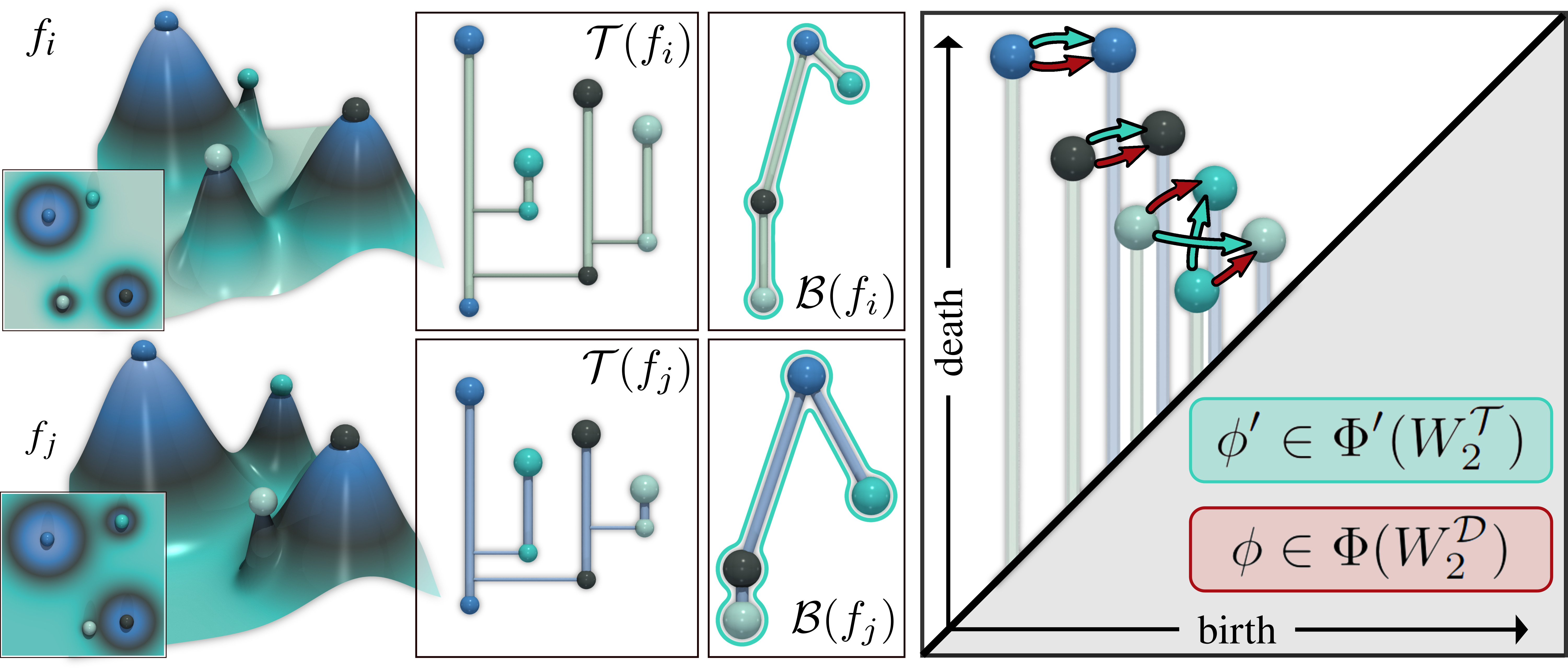
Figure 3: Illustration of the computation of the Wasserstein distance $W^{\mathcal{T}}_{2}$ [pont_vis21] between the BDTs $\mathcal{B}(f_{i})$ (white, top) and $\mathcal{B}(f_{j})$ (blue, bottom). $W^{\mathcal{T}}_{2}$ is computed by solving an optimal assignment problem in the birth/death plane (right), whose search space is constrained to partial rooted isomorphims (the optimal solution is represented with a cyan halo on the BDTs and with cyan arrows in the birth/death plane). When $\epsilon_{1}=1$, all the saddles are collapsed and the structure of the BDT is completely ignored. In that case, $W^{\mathcal{T}}_{2}$ is equal to the Wasserstein distance between persistence diagrams $W^{\mathcal{D}}_{2}$ (the optimal assignment is shown with red arrows, right). In this example, $W^{\mathcal{D}}_{2}$ reports a small distance whereas two hills have been swapped in the datasets. Figure adapted from [pont_tvcg23].

2.2 Wasserstein metric space

In this section, we first formalize the Wasserstein distance between persistence diagrams [edelsbrunner09]. Next, we recall its generalization to merge trees [pont_vis21]. This generalization enables our approach to support both topological descriptors (persistence diagrams and merge trees). This section includes elements adapted from [pont_tvcg23], which have been considered to make this manuscript self-contained.

The evaluation of the distance between two diagrams $\mathcal{D}(f_{i})$ and $\mathcal{D}(f_{j})$ is typically preceded by a pre-processing step aiming at transforming the diagrams, such that they admit the same number of points, which will facilitate the evaluation of their distance. This procedure augments each diagram with the diagonal projection of the off-diagonal points of the other diagram:

$$\mathcal{D}^{\prime}(f_{i})=\mathcal{D}(f_{i})\cup\{\Delta(p_{j})~{}|~{}p_{j}\in\mathcal{D}(f_{j})\}$$

$$\mathcal{D}^{\prime}(f_{j})=\mathcal{D}(f_{j})\cup\{\Delta(p_{i})~{}|~{}p_{i}\in\mathcal{D}(f_{i})\},$$

where $\Delta(p_{i})=(\frac{x_{i}+y_{i}}{2},\frac{x_{i}+y_{i}}{2})$ is the diagonal projection of the off-diagonal point $p_{i}=(x_{i},y_{i})$. Overall, this augmentation procedure inserts dummy features in the diagram (with zero persistence, on the diagonal), hence preserving the topological information of the diagrams, while guaranteeing that the two diagrams now have the same number of points ($|\mathcal{D}^{\prime}(f_{i})|=|\mathcal{D}^{\prime}(f_{j})|$).

In order to compare two points $p_{i}=(x_{i},y_{i})\in\mathcal{D}^{\prime}(f_{i})$ and $p_{j}=(x_{j},y_{j})\in\mathcal{D}^{\prime}(f_{j})$, a ground distance needs to be introduced in the birth/death plane. Specifically, we consider the distance $d_{q}$ ($q>0$):

$$d_{q}(p_{i},p_{j})=(|x_{j}-x_{i}|^{q}+|y_{j}-y_{i}|^{q})^{1/q}=\|p_{i}-p_{j}\|_{q}.$$

In the special case where both $p_{i}$ and $p_{j}$ are dummy features located on the diagonal (i.e. $x_{i}=y_{i}$ and $x_{j}=y_{j}$), $d_{q}(p_{i},p_{j})$ is set to zero (such that these dummy features do not intervene in the distance evaluation between the diagrams). Then, the $L^{q}$-Wasserstein distance $W^{\mathcal{D}}_{q}$ can be introduced as:

$$W^{\mathcal{D}}_{q}\big{(}\mathcal{D}(f_{i}),\mathcal{D}(f_{j})\big{)}= \underset{\phi\in\Phi}{\min} \Big{(}\sum_{p_{i}\in\mathcal{D}^{\prime}(f_{i})}d_{q}\big{(}p_{i},\phi(p_{i})\big{)}^{q}\Big{)}^{1/q},$$ (1)

where $\Phi$ is the set of all possible assignments $\phi$ mapping a point $p_{i}\in\mathcal{D}^{\prime}(f_{i})$ to a point $p_{j}\in\mathcal{D}^{\prime}(f_{j})$. Note that it is possible that $\phi$ maps a point $p_{i}\in\mathcal{D}^{\prime}(f_{i})$ to its diagonal projection (i.e. $\phi(p_{i})=\Delta(p_{i})=p_{j}\in\mathcal{D}^{\prime}(f_{j})$), which indicates the destruction of the corresponding feature (or symmetrically, its appearance).

Pont et al. recently generalized this metric to BDTs [pont_vis21]. The expression of this distance, noted $W^{\mathcal{T}}_{2}\big{(}\mathcal{B}(f_{i}),\mathcal{B}(f_{j})\big{)}$, is the same as Eq. 1 (for $q=2$), with the important difference of the search space of possible assignments, noted $\Phi^{\prime}\subseteq\Phi$. Specifically, $\Phi^{\prime}$ is constrained to the set of (rooted) partial isomorphisms [pont_vis21] between $\mathcal{B}(f_{i})$ and $\mathcal{B}(f_{j})$ (cyan halo on the BDTs of Fig. 3).

This novel metric comes with a clear interpretation. The control parameter $\epsilon_{1}$ (Sec. 2.1) balances the importance of the BDT structure in the distance. Specifically, when $\epsilon_{1}=1$, all saddles are collapsed and we have $W^{\mathcal{T}}_{2}\big{(}\mathcal{B}(f_{i}),\mathcal{B}(f_{j})\big{)}=W^{\mathcal{D}}_{2}\big{(}\mathcal{D}(f_{i}),\mathcal{D}(f_{j})\big{)}$. Generally speaking, as illustrated experimentally by Pont et al. [pont_vis21], $\epsilon_{1}$ acts as a control knob balancing the practical stability of the metric with its discriminative power. This generalized metric enables our framework to support both topological descriptors. For persistence diagrams, we set $\epsilon_{1}=1$, while for merge trees, we set it to the default recommended value (i.e. $\epsilon_{1}=0.05$ [pont_vis21]). In the following, the metric space induced by this metric is noted $\mathbb{B}$.

For interpolation purposes, Pont et al. introduce a local normalization [pont_vis21] in a pre-processing step (to guarantee the invertibility of any interpolated BDT into a valid MT). We will use the same procedure in this work to guarantee that the projected BDTs (Sec. 3.2) indeed describe valid MTs. Specifically, we normalize the persistence of each branch $b_{i}\in\mathcal{B}(f_{i})$ with regard to that of its parent $b^{\prime}_{i}\in\mathcal{B}(f_{i})$, by moving $b_{i}$ in the birth/death plane from $(x_{i},y_{i})$ to $\mathcal{N}(b_{i})=\big{(}\mathcal{N}_{x}(b_{i}),\mathcal{N}_{y}(b_{i})\big{)}$:

$$\begin{array}[]{c}\mathcal{N}_{x}(b_{i})=(x_{i}-x^{\prime}_{i})/(y^{\prime}_{i}-x^{\prime}_{i})\\ \vspace{-1.5ex}\hfil\\ \mathcal{N}_{y}(b_{i})=(y_{i}-x^{\prime}_{i})/(y^{\prime}_{i}-x^{\prime}_{i}).\end{array}$$ (5)

This pre-normalization procedure guarantees that any interpolated BDT can indeed be reverted into a valid MT, by recursively applying Eq. 5, which explicitly enforces the Elder rule [edelsbrunner09] on BDTs ($[x_{i},y_{i}]\subseteq[x^{\prime}_{i},y^{\prime}_{i}]$, Sec. 2.1), hence the validity of the reconstructed MT. Two additional parameters were introduced by Pont et al. [pont_vis21] in order to control the effect of this pre-normalization procedure ($\epsilon_{2}$ balances the normalized persistence of small branches, selected via the threshold $\epsilon_{3}$). These parameters are set to their default recommended values ($\epsilon_{2}=0.95$, $\epsilon_{3}=0.9$). In the following, we consider that all the input BDTs are pre-normalized with this procedure.

3 Formulation

This section describes our novel extension of the classical auto-encoder neural network architecture to the Wasserstein metric space of merge trees, with the novel notion of Merge Tree Wasserstein Auto-Encoder (MT-WAE). First, we describe a geometric interpretation of the classical auto-encoders (Sec. 3.1), which we call in the following Euclidean Auto-Encoders (EAE). Next, we describe how to generalize each geometrical tool used in EAE (Sec. 3.1) to the Wasserstein metric space of merge trees (Sec. 3.2). Finally, once these tools are available, we formalize our notion of MT-WAE with a novel neural network architecture (Sec. 3.3), for which we document an optimization algorithm in Sec. 4.

3.1 An interpretation of Euclidean Auto-Encoders

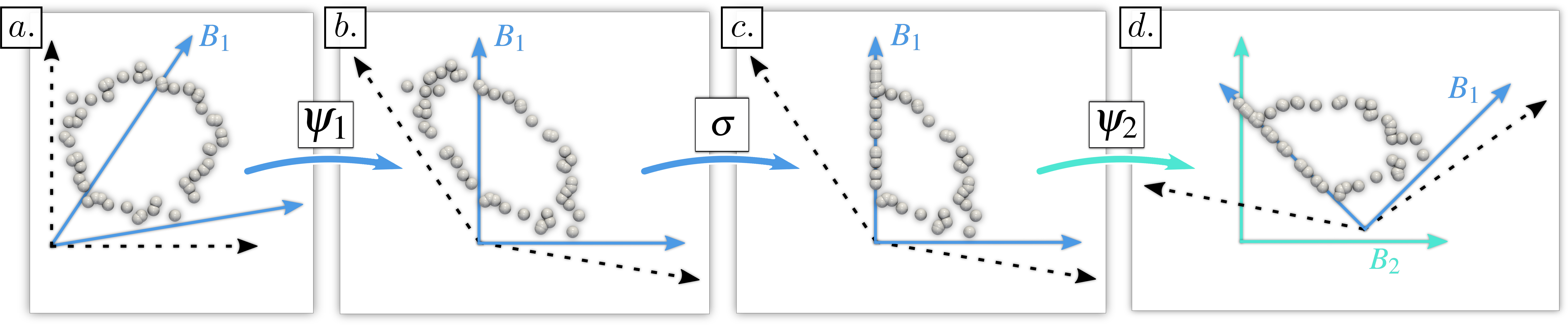
Figure 4: Geometric interpretation of Euclidean Auto-Encoders (EAE, Sec. 3.1). In its simplest form (one encoding and one decoding layer, $d^{\prime}=2$), an EAE can be viewed as the composition of a linear transformation $\psi_{1}$ $\big{(}(a)$ to $(b)\big{)}$ defined with respect to a first basis $B_{1}$, followed by a non-linearity $\sigma$ $\big{(}$here ReLU, $(b)$ to $(c)\big{)}$, followed by a second linear transformation $\psi_{2}$ $\big{(}(c)$ to $(d)\big{)}$ defined with respect to a second basis $B_{2}$. Specifically, both $\psi_{1}$ and $\psi_{2}$ are optimized (via the optimization of $B_{1}$ and $B_{2}$) to minimize the reconstruction error between the input $(a)$ and the output $(d)$. In the case where $\sigma$ is the identity, this reconstruction optimization is equivalent to Principal Component Analysis [bourlard88].

Let $P=\{p_{1},p_{2},\dots,p_{N}\}$ be a point set in a Euclidean space $\mathbb{R}^{d}$ (Fig. 4a). The goal of Euclidean Auto-Encoders (EAE) is to define a $d^{\prime}$-dimensional parameterization of $P$ (with $d^{\prime}\leq d$) which describes well the data (which enables its accurate reconstruction). Let $B_{1}=\{b_{1},b_{2},\dots,b_{d^{\prime}}\}$ be a basis of linearly independent vectors in $\mathbb{R}^{d}$ (Fig. 4a). $B_{1}$ can be written in the form of a $d\times d^{\prime}$ matrix, for which each of the $d^{\prime}$ columns is a vector of the basis. Then, one can express the coordinates $\psi_{1}(p_{i})\in\mathbb{R}^{d^{\prime}}$ of each point $p_{i}\in P$ with the basis $B_{1}$:

$$\psi_{1}(p_{i})=\argmin_{\alpha^{i}}||p_{i}-B_{1}\alpha^{i}||_{2}^{2}+o_{1},$$ (6)

where $o_{1}$ is an offset vector of $\mathbb{R}^{d^{\prime}}$, and where $\alpha^{i}\in\mathbb{R}^{d^{\prime}}$ can be seen as a set of $d^{\prime}$ coefficients, to apply on the $d^{\prime}$ vectors of the basis $B_{1}$ to best estimate $p_{i}$. Note that Eq. 6 can be re-written as a linear transformation:

$$\psi_{1}(p_{i})=B_{1}^{+}p_{i}+o_{1},$$ (7)

where $B_{1}^{+}$ is the pseudoinverse of the matrix $B_{1}$ (Figs. 4a-b).

Given this new parameterization $\psi_{1}$, one can estimate a reconstruction of the point $p_{i}$ in $\mathbb{R}^{d}$, noted $\widehat{p_{i}}$. For this, let us consider another, similar, linear transformation $\psi_{2}$ (Figs. 4c-d), defined respectively to a second basis $B_{2}$ (given as a $d^{\prime}\times d$ matrix) and a second offset vector $o_{2}$ (in $\mathbb{R}^{d}$). Then, the reconstruction $\widehat{p_{i}}$ of each point $p_{i}$ is given by:

$$\widehat{p_{i}}=\psi_{2}\circ\psi_{1}(p_{i})=B_{2}^{+}(B_{1}^{+}p_{i}+o_{1})+o_{2}.$$

To get an accurate reconstruction $\widehat{p_{i}}$ (Fig. 4d) for all the points $p_{i}\in P$, one needs to optimize both $\psi_{1}$ and $\psi_{2}$, to minimize the following data fitting energy:

$$E_{L_{2}}=\sum_{i=1}^{N}||p_{i}-\widehat{p_{i}}||_{2}^{2}=\sum_{i=1}^{N}||p_{i}-\psi_{2}\circ\psi_{1}(p_{i})||_{2}^{2}.$$ (8)

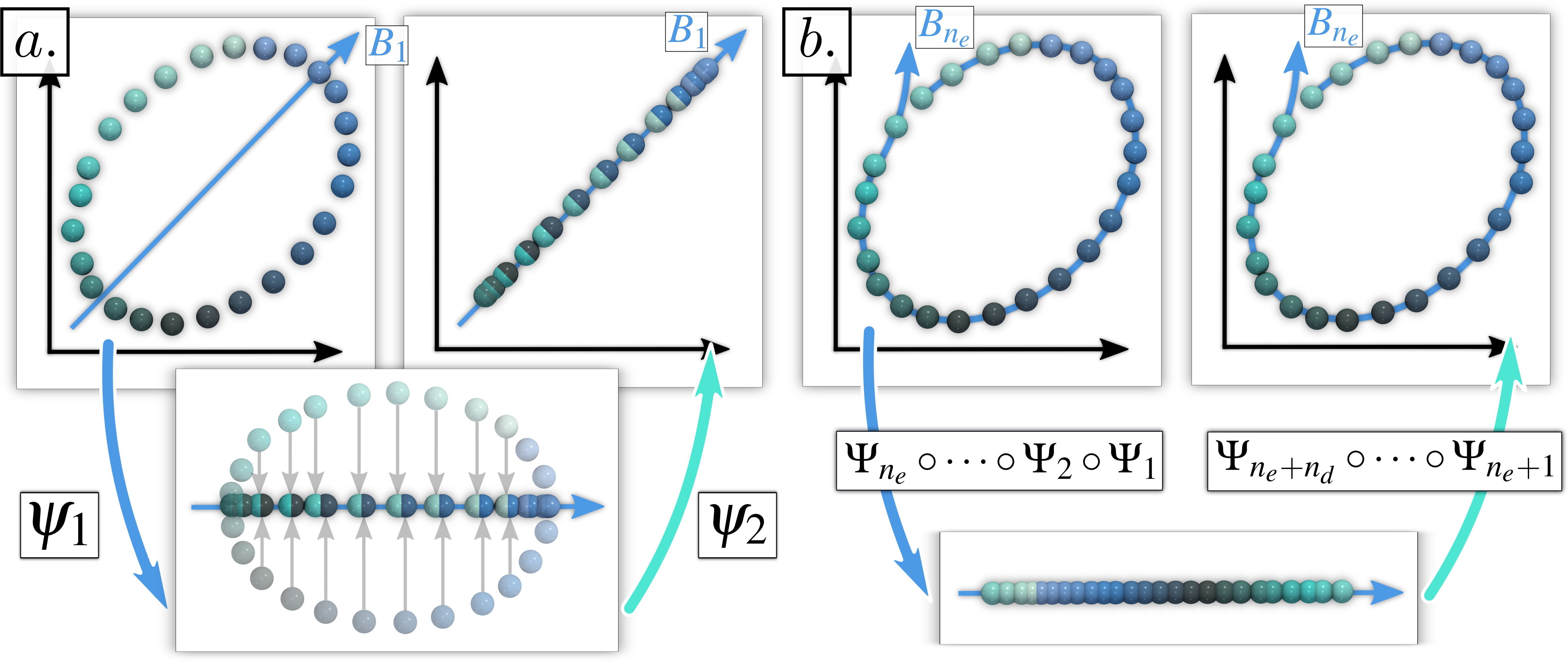
Figure 5: Comparison between PCA $(a)$ and EAE $(b)$ for the $1$-dimensional encoding of a 2D point set sampling a $1$-manifold (color: rotation angle). In its latent space $\big{(}(a)$, bottom$\big{)}$, PCA linearly projects the input points to a line, hence interleaving points from the upper and lower parts of the circle. This results in a poor reconstruction $\big{(}(a)$, right$\big{)}$, where points are interleaved along the axis $B_{1}$. In contrast, EAE optimizes a composition of non-linear transformations, which consistently unwraps the circle onto a line in its latent space $\big{(}(b)$, bottom$\big{)}$, while nicely preserving the intrinsic parameterization of the circle (rotation angle). This results in an accurate reconstruction $\big{(}(b)$, right$\big{)}$: the embedding of the axis $B_{n_{e}}$ in the data defines a faithful $1$-dimensional parameterization of the circle.

As discussed by Bourlard and Kamp [bourlard88], this formulation is a generalization of Principal Component Analysis (PCA) [pearson01], a seminal statistical tool for variability analysis. However, PCA assumes that the input point cloud can be faithfully approximated via linear projections. As shown in Fig. 5, this hypothesis can be easily challenged in practice. This motivates a non-linear generalization of PCA, capable of faithfully approximating point clouds exhibiting non-linear structures (Fig. 5).

Specifically, to introduce non-linearity, the above linear transformations $\psi$ are typically composed with a non-linear function $\sigma$, called activation function, such that the transformation of each point $p_{i}$, noted $\Psi(p_{i})$, is now given by: $\Psi(p_{i})=\sigma\big{(}\psi(p_{i})\big{)}$. For example, the rectifier activation function (“ReLU”) will take the $j^{th}$ coordinate of each data point (i.e. $\big{(}\psi(p_{i})\big{)}_{j}$) and snap it to zero if it is negative (Fig. 4b-c). We call the above non-linear transformation $\Psi$ a transformation layer. It is characterized by its own vector basis $B$ and its own offset vector $o$.

Next, to faithfully approximate complicated non-linear input distributions, the above transformation layer is typically composed with a number ($n_{e}+n_{d}$) of other transformation layers, defined similarly. Then, the initial data fitting energy (Eq. 8) can now be generalized into:

$$E_{L_{2}}=\sum_{i=1}^{N}||p_{i}-\Psi_{n_{e}+n_{d}}\circ\dots\circ\Psi_{n_{e}+1}\circ\Psi_{n_{e}}\circ\dots\circ\Psi_{2}\circ\Psi_{1}(p_{i})||_{2}^{2},$$ (9)

where each transformation layer $\Psi_{k}$ is associated with its own $d_{k}$-dimensional vector basis $B_{k}$ and its offset vector $o_{k}$. Then, the notion of Auto-Encoder is a specific instance of the above formulation, with:

1. $d_{1}>d_{2}>\dots>d_{n_{e}}$, and

2. $d_{n_{e}}<d_{n_{e}+1}<\dots<d_{n_{e}+n_{d}}=d$, and

3. $\sigma_{n_{e}+n_{d}}$ is the identity.

Specifically, $n_{e}$ and $n_{d}$ respectively denote the number of Encoding and Decoding transformation layers, while $d_{n_{e}}$ is the dimension of the so-called latent space. In practice, $d_{n_{e}}$ is typically chosen to be much smaller than the input dimensionality ($d$), for non-linear dimensionality reduction purposes (each input point $p_{i}$ is then represented in $d_{n_{e}}$ dimensions, according to its coordinates in $B_{n_{e}}$, noted $\alpha_{n_{e}}^{i}\in\mathbb{R}^{d_{n_{e}}}$).

Eq. 9 defines an optimization problem whose variables (the $n_{e}+n_{d}$ bases and offset vectors) can be efficiently optimized (e.g. with gradient descent [KingmaB14]) by composing the transformation layers within a neural network. Then, the gradient $\nabla E_{L_{2}}$ of $E_{L_{2}}$ can be estimated by exploiting the automatic differentiation capabilities of modern neural network implementations [pytorch], themselves based on the application of the chain-rule derivation on the above composition of transformation layers.

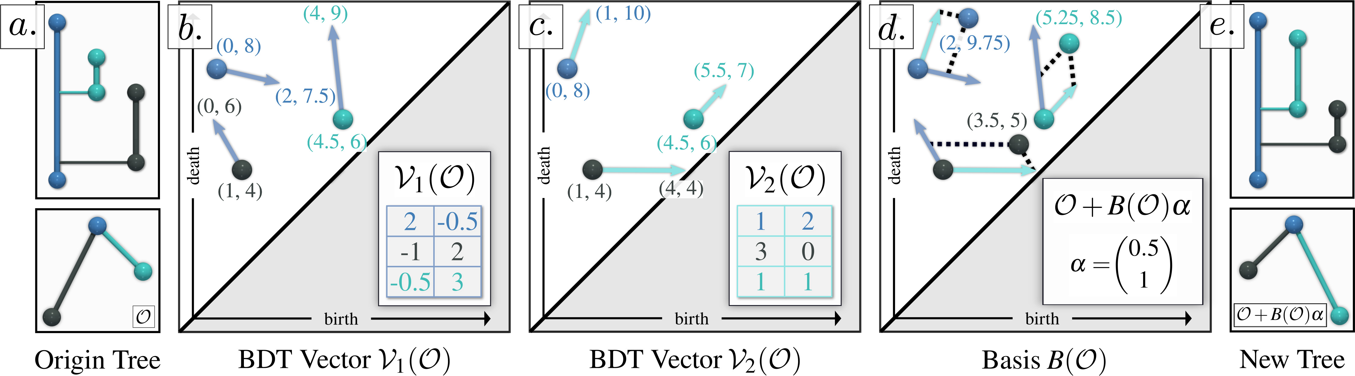
Figure 6: Low-level geometrical tools in the Wasserstein metric space of merge trees (Sec. 3.2). Given an origin MT and its BDT $\mathcal{O}$ $\big{(}$counting $|\mathcal{O}|$ nodes $(a)\big{)}$, a BDT vector $\mathcal{V}_{1}(\mathcal{O})$ is defined in the birth/death space as a concatenation of $|\mathcal{O}|$ 2D vectors $\big{(}$blue arrows $(b)\big{)}$. Given a second BDT vector $\mathcal{V}_{2}(\mathcal{O})$ $\big{(}$cyan arrows $(c)\big{)}$, a basis $B(\mathcal{O})$ can be defined $\big{(}(d)$, here with $d^{\prime}=2\big{)}$. For a given set of coefficients $\alpha\in\mathbb{R}^{d^{\prime}}$, a new merge tree and its BDT $(e)$ can be reconstructed by applying a sum of 2D displacements $\sum_{j=1}^{j=d^{\prime}}\alpha_{j}\big{(}\mathcal{V}_{j}(\mathcal{O})\big{)}_{i}$ to each branch $b_{i}$ of $\mathcal{O}$ $\big{(}(d)$, black dashes$\big{)}$.

3.2 From EAE to MT-WAE

When the input data is not given as a point cloud in a Euclidean space (Sec. 3.1) but as an abstract set equipped with a metric, the above EAE formulation needs to be extended. For this, we redefine in this section the low-level geometrical tools used in EAE (Sec. 3.1), but within the context of the Wasserstein metric space $\mathbb{B}$ [pont_vis21]. In particular, we formalize the following notions:

1. BDT vector (Fig. 6b);

2. BDT basis (Fig. 6d);

3. BDT basis projection (Fig. 6d);

4. BDT transformation layer (Fig. 7b).

(1) BDT vector: Given a BDT $\mathcal{B}$ with $|\mathcal{B}|$ branches, a BDT vector $\mathcal{V}(\mathcal{B})\in\mathbb{B}$ is a vector in $\mathbb{R}^{2|\mathcal{B}|}$, which maps each branch $b\in\mathcal{B}$ to a new location in the 2D birth/death space. $\mathcal{B}$ is the origin of $\mathcal{V}(\mathcal{B})$. This is illustrated for example in Fig. 6b), where the branches of a given merge tree $\big{(}$Fig. 6a$\big{)}$ are displaced in the birth-death plane (light blue vectors from the spheres of matching color).

(2) BDT basis: Given an origin BDT $\mathcal{O}$, a $d^{\prime}$-dimensional basis of BDT vectors, noted $B(\mathcal{O})$, is a set $\{\mathcal{V}_{1}(\mathcal{O}),\mathcal{V}_{2}(\mathcal{O}),\dots,\mathcal{V}_{d^{\prime}}(\mathcal{O})\}$ of $d^{\prime}$ linearly independent BDT vectors, having for common origin $\mathcal{O}$. This is shown in Fig. 6d), where two BDT vectors (from Fig. 6b), and Fig. 6c), blue and green arrows) are combined into a basis. Sec. 4.3 clarifies the basis initialization by our approach.

(3) BDT basis projection: Given an arbitrary BDT $\mathcal{B}$, its projection error $e(\mathcal{B})$ in a $d^{\prime}$-dimensional BDT basis $B(\mathcal{O})$ is:

$$e(\mathcal{B})=\min_{\alpha}\Big{(}W^{\mathcal{T}}_{2}\big{(}\mathcal{B},\mathcal{O}+B(\mathcal{O})\alpha\big{)}\Big{)}^{2},$$ (10)

where $\alpha\in\mathbb{R}^{d^{\prime}}$ can be interpreted as a set of coefficients to apply on the $d^{\prime}$ BDT vectors of $B(\mathcal{O})$ to best estimate $\mathcal{B}$. Then, the projection of $\mathcal{B}$ in $B(\mathcal{O})$, noted $\psi(\mathcal{B})$, is given by the optimal coefficients $\alpha$ associated to the projection error of $\mathcal{B}$ (Eq. 10):

$$\psi(\mathcal{B})=\argmin_{\alpha}\Big{(}W^{\mathcal{T}}_{2}\big{(}\mathcal{B},\mathcal{O}+B(\mathcal{O})\alpha\big{)}\Big{)}^{2}.$$ (11)

The above equation is a re-interpretation of Eq. 6 (Sec. 3.1), where the $L_{2}$ norm (used for EAE) is replaced by the Wasserstein distance $W^{\mathcal{T}}_{2}$. This projection procedure is illustrated in Fig. 6d). Given a BDT basis $B(\mathcal{O})$ (blue and green arrows), the projection of an arbitrary BDT $\mathcal{B}$ is the linear combination $\psi(\mathcal{B})$ of the BDT vectors of the basis which minimizes its Wasserstein distance $W^{\mathcal{T}}_{2}$ to $\mathcal{B}$. In the birth-death space, the branches of the basis origin $\mathcal{O}$ are represented by the colored spheres at the intersection between the blue and green arrows, while the branches of $\psi(\mathcal{B})$ are represented by the other spheres of matching color. In this example, the linear combination $\psi(\mathcal{B})$ which minimizes its distance to $\mathcal{B}$ is obtained for the coefficients $\alpha=(0.5,1)$. Then, to go from $\mathcal{O}$ to $\psi(\mathcal{B})$, each branch $b_{i}$ of $\mathcal{O}$ is displaced by $0.5~{}\mathcal{V}_{1}(\mathcal{O})$ (intersection between the dashed lines and the blue arrows) and then by $1~{}\mathcal{V}_{2}(\mathcal{O})$ (intersection between the dashed lines and the green arrows). The resulting merge tree is shown in Fig. 6e). In contrast to the merge tree of the basis origin $\big{(}$Fig. 6a)$\big{)}$, the persistence of the cyan branch has increased while that of the black branch has decreased.

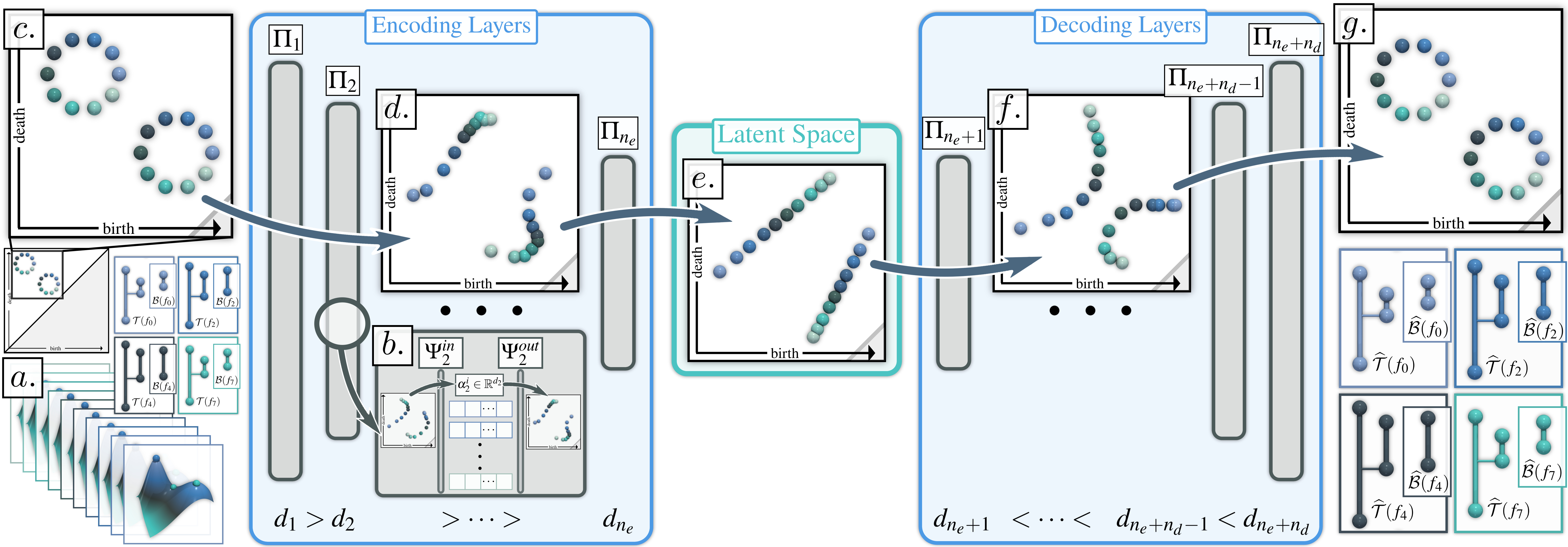
Figure 7: Overview: given an input ensemble, with its merge trees and BDTs $(a)$, our Wasserstein Auto-Encoder of Merge Trees (MT-WAE) optimizes an auto-encoder (for this example, $n_{e}=n_{d}=2$) where each layer $\Pi_{k}$ natively processes BDTs (without pre-vectorization). Specifically, each layer $\Pi_{k}$ can be interpreted as a local auto-encoder $(b)$, where an input sub-layer $\Psi_{k}^{in}$ transforms the input BDT $\mathcal{B}_{k-1}(f_{i})$ into a set of coefficients $\alpha_{k}^{i}\in\mathbb{R}^{d_{k}}$ and where an output sub-layer $\Psi_{k}^{out}$ transforms these coefficients back into a valid BDT $\mathcal{B}_{k}(f_{i})$. The aggregated views $\big{(}(c),(d),(e),(f),(g)\big{)}$, which overlap all the BDTs in the birth/death space (one color per BDT), show the ability of MT-WAE to progressively unwrap non-linear structures (circles) as the BDTs progress down the network, resulting in faithful local parameterizations in latent space $\big{(}(e)$, the individual angular parameterizations of the circles are well preserved$\big{)}$, as well as accurate reconstructions $(g)$. This native support of BDTs results in a superior accuracy (Sec. 6.2) and an improved interpretability: individual features can now be tracked as they traverse the network, enabling new visual analysis capabilities (Sec. 5.2).

(4) BDT transformation layer: Once the above tools have been formalized, we can introduce the novel notion of BDT transformation layer. Similarly to the Euclidean case (Sec. 3.1), a non-linear activation function $\sigma$ (in our case, Leaky ReLU) can be composed with the above projection, yielding the new function $\Psi(\mathcal{B})=\sigma\big{(}\psi(\mathcal{B})\big{)}$. Note that, at this stage, $\Psi(\mathcal{B})$ can be interpreted as a set of coefficients to apply on the BDT basis $B(\mathcal{O})$ to best estimate $\mathcal{B}$. In other words, $\Psi(\mathcal{B})$ is not a BDT yet, but simply a set of coefficients, which can be used later to reconstruct a BDT. Thus, a second transformation needs to be considered, to transform the set of coefficients $\Psi(\mathcal{B})$ back into a BDT. Then, we define the notion of BDT transformation layer, noted $\Pi(\mathcal{B})$, as the composition $\Pi(\mathcal{B})=\Psi^{out}\circ\Psi^{in}(\mathcal{B})$ (Fig. 7b):

$$\begin{array}[]{l}\Psi^{in}(\mathcal{B})=\sigma\bigg{(}\argmin_{\alpha}\Big{(}W^{\mathcal{T}}_{2}\big{(}\mathcal{B},\mathcal{O}^{in}+B^{in}(\mathcal{O}^{in})\alpha\big{)}\Big{)}^{2}\bigg{)}\\ \Psi^{out}(\alpha)=\gamma\big{(}\mathcal{O}^{out}+B^{out}(\mathcal{O}^{out})\alpha\big{)},\end{array}$$ (14)

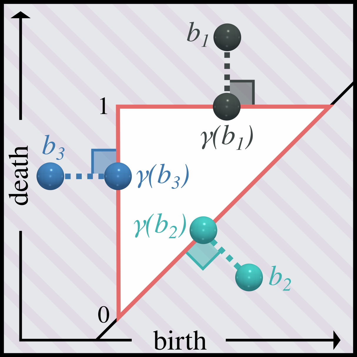
Figure 8: Projection $\gamma$ ensuring the Elder rule.

where $\gamma(\mathcal{B})$ is a projection which transforms $\mathcal{B}$ into a valid BDT, i.e. which respects the Elder rule (Sec. 2.1). Given a branch $b\in\mathcal{B}$, $\gamma$ enforces that: $\gamma(b)_{x}<\gamma(b)_{y}$ and $[\gamma(b)_{x},\gamma(b)_{y}]\subseteq[0,1]$ (Fig. 8).

BDT transformation layers can be seen as local auto-encoders (Fig. 7b): the first step $\Psi^{in}$ converts an input BDT into a set of coefficients with a basis projection and a non-linearity, while the second step $\Psi^{out}$ converts these coefficients into a BDT. Note that each BDT transformation layer is associated with its own input and output $d^{\prime}$-dimensional bases $B^{in}(\mathcal{O}^{in})$ and $B^{out}(\mathcal{O}^{out})$.

The processing of an ensemble of BDTs by a BDT transformation layer is illustrated in Fig. 7. Specifically, Fig. 7c) shows a zoom of the birth-death space, where all the BDTs have been aggregated (one color per BDT, each BDT has two branches, hence two patterns appear, one circle per branch). The left inset of Fig. 7b) shows the non-linearly transformed set of BDTs after the first BDT transformation layer, $\Pi_{1}$. Next, the first step $\Psi^{in}_{2}$ of the next BDT layer $\Pi_{2}$ converts each BDT $\Pi_{1}\big{(}\mathcal{B}(f_{i})\big{)}$ into a set of coefficients $\alpha_{2}^{i}$. Finally, the second step $\Psi^{out}_{2}$ of the layer $\Pi_{2}$ converts each of these set of coefficients into a new, non-linearly transformed BDT $\Pi_{2}\circ\Pi_{1}\big{(}\mathcal{B}(f_{i})\big{)}$ $\big{(}$Fig. 7b), right inset$\big{)}$.

3.3 MT-WAE formulation

Now that the above geometrical tools have been introduced for the Wasserstein metric space of merge trees, we can now formulate MT-WAE by direct analogy to the Euclidean case (Sec. 3.1). Given a set $\mathcal{S}_{\mathcal{B}}=\{\mathcal{B}(f_{1}),\dots,\mathcal{B}(f_{N})\}$ of input BDTs, a MT-WAE is a composition of BDT transformation layers $\Pi_{k}(\mathcal{B})$ (Fig. 7), minimizing the following energy:

$$E_{W^{\mathcal{T}}_{2}}=\sum_{i=1}^{N}\bigg{(}W^{\mathcal{T}}_{2}\Big{(}\mathcal{B}(f_{i}),\Pi_{n_{e}+n_{d}}\circ\dots\circ\Pi_{n_{e}}\circ\dots\circ\Pi_{1}\big{(}\mathcal{B}(f_{i})\big{)}\Big{)}\bigg{)}^{2},$$ (15)

where each BDT transformation layer $\Pi_{k}$ is associated with its own $d_{k}$-dimensional input and output vector bases $B^{in}_{k}(\mathcal{O}_{k}^{in})$ and $B^{out}_{k}(\mathcal{O}_{k}^{out})$. Moreover, the dimensions of the successive bases are chosen such that:

1. $d_{1}>d_{2}>\dots>d_{n_{e}}$, and

2. $d_{n_{e}}<d_{n_{e}+1}<\dots<d_{n_{e}+n_{d}}$,

where $n_{e}$ and $n_{d}$ denote the number of Encoding and Decoding layers and where $d_{n_{e}}$ is the dimension of the MT-WAE latent space. Eq. 15 is a direct analog to the classical EAE (Eq. 9): the standard transformation layers $\Psi_{k}$ have been replaced by BDT transformation layers $\Pi_{k}$ and the $L_{2}$ norm by the distance $W^{\mathcal{T}}_{2}$.

Fig. 7 illustrates a network of BDT transformation layers optimized on a synthetic ensemble (our optimization algorithm is described in Sec. 4). As mentioned in the previous section, each input BDT (spheres in the aggregated birth-death views, one color per BDT) is non-linearly transformed by the BDT transformation layers $\big{(}$see for instance Fig. 7d) and Fig. 7f)$\big{)}$. As a result, in this example, the BDT transformation layers progressively unwrap the non-linear structures in the birth-death plane $\big{(}$circles in Fig. 7c)$\big{)}$ as the BDTs traverse the network down to the latent space $\big{(}$Fig. 7e)$\big{)}$, where the resulting layout in the birth-death plane (line segments) manages to faithfully encode the purposely designed parameterization of the ensemble: the order of rotation angles (colors) is well preserved along the segments in latent space.

4 Algorithm

This section presents our algorithm for the minimization of Eq. 15.

Algorithm 1 Wasserstein Auto-Encoder (algorithm overview).

Input: Set of BDTs $\mathcal{S}_{\mathcal{B}}=\{\mathcal{B}(f_{1}),\dots,\mathcal{B}(f_{N})\}$.

Output1: Set of $(n_{e}+n_{d})$ input origins $\theta_{\mathcal{O}^{in}}=\{\mathcal{O}^{in}_{1},\mathcal{O}^{in}_{2},\dots,\mathcal{O}^{in}_{n_{e}+n_{d}}\}$;

Output2: Set of $(n_{e}+n_{d})$ input bases $\theta_{B^{in}}=\{B^{in}_{1}(\mathcal{O}^{in}_{1}),B^{in}_{2}(\mathcal{O}^{in}_{2}),\dots,B^{in}_{n_{e}+n_{d}}(\mathcal{O}^{in}_{n_{e}+n_{d}})\}$;

Output3: For each of the input BDTs ($i\in\{1,2,\dots,N\}$), set of $(n_{e}+n_{d})$ input coefficients:
        $\theta_{\alpha}^{i}=\{\alpha_{1}^{i}\in\mathbb{R}^{d_{1}},\alpha_{2}^{i}\in\mathbb{R}^{d_{2}},\dots,\alpha_{n_{e}+n_{d}}^{i}\in\mathbb{R}^{d_{n_{e}+n_{d}}}\}$;

Output4: Set of $(n_{e}+n_{d})$ output origins $\theta_{\mathcal{O}^{out}}=\{\mathcal{O}^{out}_{1},\mathcal{O}^{out}_{2},\dots,\mathcal{O}^{out}_{n_{e}+n_{d}}\}$;

Output5: Set of $(n_{e}+n_{d})$ output bases $\theta_{B^{out}}=\{B^{out}_{1}(\mathcal{O}^{out}_{1}),B^{out}_{2}(\mathcal{O}^{out}_{2}),\dots,B^{out}_{n_{e}+n_{d}}(\mathcal{O}^{out}_{n_{e}+n_{d}})\}$;

1:  $\theta\leftarrow\{\theta_{\mathcal{O}^{in}},\theta_{B^{in}},\theta_{\mathcal{O}^{out}},\theta_{B^{out}}\};$ / / Overall set of optimization variables.

2:  Initialize$(\theta);$ / / Initialization of the optimization variables (Sec. 4.3).

3:  while $E_{W^{\mathcal{T}}_{2}}(\theta)$ decreases do

4:     $\widehat{\mathcal{S}_{\mathcal{B}}}\leftarrow$ Forward$(\mathcal{S}_{\mathcal{B}},\theta);$ / / Forward propagation of the BDT ensemble $\mathcal{S}_{\mathcal{B}}$ (Sec. 4.4).

5:     $\theta\leftarrow$ Backward$(\mathcal{S}_{\mathcal{B}},\widehat{\mathcal{S}_{\mathcal{B}}});$ / / Backward propagation (Sec. 4.5).

6:  end while

4.1 Overview

Alg. 1 provides an overview of our main algorithm. The set of optimization variables, noted $\theta$ and declared line 1, includes the $(n_{e}+n_{d})$ input and output BDT bases, along with their origins. The optimization of these variables follows the standard overall procedure for the optimization of a neural network.

(1) Initialization: First, $\theta$ is initialized, as detailed in Sec. 4.3.

(2) Forward propagation: Then, the input ensemble of BDTs $\mathcal{S}_{\mathcal{B}}$, illustrated in Fig. 7a, traverses the network to generate a reconstructed ensemble of BDTs, noted $\widehat{\mathcal{S}_{\mathcal{B}}}$. This occurs line 4 of Alg. 1 and it is illustrated from Fig. 7c to Fig. 7g with the dark blue arrows. This is traditionally denoted as the Forward propagation. This part of our approach is documented in Sec. 4.4.

(3) Backward propagation: Given $\widehat{\mathcal{S}_{\mathcal{B}}}$, the energy $E_{W^{\mathcal{T}}_{2}}(\theta)$, detailed in Eq. 15, can be evaluated and its gradient $\nabla E_{W^{\mathcal{T}}_{2}}(\theta)$ can be estimated by automatic differentiation, based on the application of the chain-rule on the composition of BDT transformation layers. Given the gradient $\nabla E_{W^{\mathcal{T}}_{2}}(\theta)$, a step of gradient descent can be achieved to update the optimization variables $\theta$. This occurs line 5 of Alg. 1. This is traditionally denoted as the Backward propagation. This part of our approach is detailed in Sec. 4.5.

(4) Stopping condition: The two steps of forward and backward propagations are then iterated until the energy stops decreasing, in practice until it decreases by less than $1\%$ between two iterations.

4.2 Basis projection

We start by describing an efficient Assignment/Update algorithm for the projection of a BDT $\mathcal{B}$ into a BDT basis $B(\mathcal{O})$ (Eq. 11), as it is a core geometrical component used throughout our approach.

The purpose of the projection (Eq. 11) is to find a set of coefficients $\alpha\in\mathbb{R}^{d^{\prime}}$ to apply on the $d^{\prime}$ BDT vectors of $B(\mathcal{O})$ to best estimate $\mathcal{B}$. The geodesic analysis of merge trees [pont_tvcg23] faces a similar issue, but its formulation (restricting $\alpha$ to $[0,1]^{d^{\prime}}$) allows for an iterative, brute-force optimization. Here, we introduce a more general and efficient strategy.

(1) Assignment step: Let us assume that we are given an initial set of coefficients $\alpha$. Then, the estimation $\widehat{\mathcal{B}}$ of $\mathcal{B}$ is given by $\widehat{\mathcal{B}}\leftarrow\mathcal{O}+B(\mathcal{O})\alpha$. The purpose of the assignment step is to refine the evaluation of $W^{\mathcal{T}}_{2}(\mathcal{B},\widehat{\mathcal{B}})$. For this, we first compute the optimal assignment $\phi_{*}$ between $\mathcal{B}$ and $\widehat{\mathcal{B}}$, w.r.t. Eq. 1. Then, $W^{\mathcal{T}}_{2}(\mathcal{B},\widehat{\mathcal{B}})$ can be re-written as:

$$W^{\mathcal{T}}_{2}(\mathcal{B},\widehat{\mathcal{B}})=\sum_{i=1}^{|\mathcal{B}|}||b_{i}-\phi_{*}(b_{i})||_{2}^{2}.$$ (16)

(2) Update step: Given the above estimation $\widehat{\mathcal{B}}$, the goal of the update step is to improve the coefficients $\alpha$, in order to decrease $W^{\mathcal{T}}_{2}(\mathcal{B},\widehat{\mathcal{B}})$. Let $\widehat{\mathcal{B}^{\prime}}$ be a vector representation of $\widehat{\mathcal{B}}$. Specifically, $\widehat{\mathcal{B}^{\prime}}$ is a vector in $\mathbb{R}^{2|\widehat{\mathcal{B}}|}$ which concatenates the coordinates in the 2D birth/death plane of each branch $b_{i}$ of $\widehat{\mathcal{B}}$. $\widehat{\mathcal{B}^{\prime}}$ can be decomposed into $\mathcal{O}^{\prime}+\big{(}B(\mathcal{O}^{\prime})\big{)}^{\prime}\alpha$, where $\big{(}B(\mathcal{O}^{\prime})\big{)}^{\prime}$ is a $(2|\widehat{\mathcal{B}}|)\times d^{\prime}$ matrix. Additionally, let $\mathcal{B}^{\prime}$ be a similar vector representation of $\mathcal{B}$, but where the entries have been specifically re-ordered such that, for each of its 2D entries, we have:

$$(\mathcal{B}^{\prime})_{i}=\phi_{*}^{-1}\big{(}(\widehat{\mathcal{B}^{\prime}})_{i}\big{)}.$$ (17)

Intuitively, $\mathcal{B}^{\prime}$ is a re-ordered vector representation of $\mathcal{B}$, such that its $i^{th}$ entry exactly matches though $\phi_{*}$ with the $i^{th}$ entry of $\widehat{\mathcal{B}^{\prime}}$. Given this vector representation, the Wasserstein distance $W^{\mathcal{T}}_{2}(\mathcal{B},\widehat{\mathcal{B}})$ for a fixed optimal assignment $\phi^{*}$ (Eq. 16) can then be re-written as an $L_{2}$ norm:

$$W^{\mathcal{T}}_{2}(\mathcal{B},\widehat{\mathcal{B}})=||\mathcal{B}^{\prime}-\widehat{\mathcal{B}^{\prime}}||_{2}^{2}.$$ (18)

Then, given the optimal assignment $\phi_{*}$, the optimal $\alpha_{*}\in\mathbb{R}^{d^{\prime}}$ are:

$$\begin{array}[]{lll}\alpha_{*}&=&\argmin_{\alpha}||\mathcal{B}^{\prime}-\widehat{\mathcal{B}^{\prime}}||_{2}^{2}\\ \alpha_{*}&=&\argmin_{\alpha}||\mathcal{B}^{\prime}-\Big{(}\mathcal{O}^{\prime}+\big{(}B(\mathcal{O}^{\prime})\big{)}^{\prime}\alpha\Big{)}||_{2}^{2}\\ \alpha_{*}&=&\argmin_{\alpha}||\mathcal{B}^{\prime}-\mathcal{O}^{\prime}-\big{(}B(\mathcal{O}^{\prime})\big{)}^{\prime}\alpha||_{2}^{2}.\end{array}$$ (22)

Similarly to the Euclidean case (Eq. 7), it follows then that $\alpha_{*}$ can be expressed as a function of the pseudoinverse of $\big{(}B(\mathcal{O}^{\prime})\big{)}^{\prime}$:

$$\alpha_{*}=\Big{(}\big{(}B(\mathcal{O}^{\prime})\big{)}^{\prime}\Big{)}^{+}(\mathcal{B}^{\prime}-\mathcal{O}^{\prime}).$$ (23)

At this stage, the estimation $\widehat{\mathcal{B}}$ can be updated with the above optimized coefficients $\alpha_{*}$: $\widehat{\mathcal{B}}\leftarrow\mathcal{O}+B(\mathcal{O})\alpha_{*}$.

The above Assignment/Update sequence is then iterated. Each iteration decreases the projection error $e(\mathcal{B})$ constructively: while the Update phase (2) optimizes $\alpha$ (Eq. 10) to minimize the projection error under the current assignment $\phi_{*}$, the next Assignment phase (1) further improves (by construction) the assignments (term $W^{\mathcal{T}}_{2}$ in Eq. 10), hence decreasing the projection error overall. In our implementation, this iterative algorithm stops after a predefined number of iterations $n_{it}$.

4.3 Initialization

Now that we have introduced the core low-level procedure of our approach (Sec. 4.2), we can detail the initialization step of our framework, which consists in identifying a relevant initial value for the overall optimization variable $\theta$ (line 2, Alg. 1). The BDT transformation layers $\Pi_{k}$ are initialized one after the other, i.e. for increasing values of $k$.

(1) Input initialization: For each BDT transformation layer $\Pi_{k}$, its input origin $\mathcal{O}_{k}^{in}$ is initialized as the Wasserstein barycenter $\mathcal{B}_{*}$ [pont_vis21] of the BDTs on its input. Next, the first vector of $B_{k}^{in}$, is given by the optimal assignment (w.r.t. Eq. 1) between $\mathcal{O}_{k}^{in}$ and the layer’s input BDT $\mathcal{B}$ which maximizes $W^{\mathcal{T}}_{2}(\mathcal{O}_{k}^{in},\mathcal{B})$, i.e. which induces the worst projection error $e(\mathcal{B})$ (Eq. 10) given an empty basis. Next, the remaining $(d_{k}-1)$ vectors of $B_{k}^{in}$ are initialized one after the other, by including at each step the vector formed by the optimal assignment between $\mathcal{O}_{k}^{in}$ and the layer’s input BDT $\mathcal{B}$ which induces the maximum projection error $e(\mathcal{B})$ (Eq. 10), given the already initialized vectors. Note that this step makes an extensive usage of the projection procedure introduced in Sec. 4.2. Finally, if the dimension $d_{k}$ of $\Pi_{k}$ is greater than the number of input BDTs, the remaining vectors are initialized randomly, with a controlled norm (set to the mean of the already initialized vectors).

(2) Output initialization: For each BDT transformation layer $\Pi_{k}$, its output origin $\mathcal{O}_{k}^{out}$ and basis $B_{k}^{out}$ are initialized as random linear transformations of its input origin and basis. Specifically, let $W$ be a random matrix of size $(2|\mathcal{O}_{k}^{out}|\times 2|\mathcal{O}_{k}^{in}|)$. Given the vector representation ${\mathcal{O}_{k}^{in}}^{\prime}$ of $\mathcal{O}_{k}^{in}$ (see Sec. 4.2), we initialize $\mathcal{O}_{k}^{out}$ such that: ${\mathcal{O}_{k}^{out}}^{\prime}\leftarrow W{\mathcal{O}_{k}^{in}}^{\prime}$. Similarly, the output basis of $\Pi_{k}$ is initialized such that: ${B_{k}^{out}}^{\prime}\leftarrow W{B_{k}^{in}}^{\prime}$.

Algorithm 2 Forward propagation in our Wasserstein Auto-Encoder.

Input1: Set of input BDTs $\mathcal{S}_{\mathcal{B}}=\{\mathcal{B}(f_{1}),\dots,\mathcal{B}(f_{N})\}$.

Input2: Current value of the overall optimization variable $\theta$.

Output: Set of reconstructed BDTs $\widehat{\mathcal{S}_{\mathcal{B}}}=\{\widehat{\mathcal{B}(f_{1})},\dots,\widehat{\mathcal{B}(f_{N})}\}$.

1:  for $\mathcal{B}\in\mathcal{S}_{\mathcal{B}}$ do

2:     $\mathcal{B}_{0}\leftarrow\mathcal{B}$.

3:     for $k\in\{1,2,\dots,n_{e}+n_{d}\}$ do

4:        // For each BDT transformation layer $\Pi_{k}$.

5:        $\psi_{k}^{in}(\mathcal{B}_{k-1})\leftarrow$basisProjection$(\mathcal{B}_{k-1},\mathcal{O}_{k}^{in},B_{k}^{in}).$ / / Sec. 4.2.

6:        $\Psi_{k}^{in}(\mathcal{B}_{k-1})\leftarrow\sigma\big{(}\psi_{k}^{in}(\mathcal{B}_{k-1})\big{)}$. / / Sec. 3.2.

7:        $\mathcal{B}_{k}\leftarrow\Psi_{k}^{out}\big{(}\Psi_{k}^{in}(\mathcal{B}_{k-1})\big{)}=\gamma\big{(}\mathcal{O}_{k}^{out}+B_{k}^{out}(\mathcal{O}_{k}^{out})\Psi_{k}^{in}(\mathcal{B}_{k-1})\big{)}.$ / / Sec. 3.2.

8:     end for

9:     $\widehat{\mathcal{S}_{\mathcal{B}}}\leftarrow\widehat{\mathcal{S}_{\mathcal{B}}}\cup\mathcal{B}_{n_{e}+n_{d}}$

10:  end for

4.4 Forward propagation

Alg. 2 presents the main steps of our forward propagation. This procedure follows directly from our formulation (Sec. 3.2). Each input BDT $\mathcal{B}\in\mathcal{S}_{\mathcal{B}}$ is processed independently (line 1). Specifically, $\mathcal{B}$ will traverse the network one layer $\Pi_{k}$ at a time (line 3). Within each layer $\Pi_{k}$, the projection through the input sub-layer $\Psi_{k}^{in}$ is computed (line 6) by composing a non-linearity $\sigma$ with the basis projection (Sec. 3.2). This yields a set of coefficients representing the input BDT. Next, following Sec. 3.2, these coefficients are transformed back into a valid BDT with the output sub-layer (line 7). At the end of this process, a set of reconstructed BDTs $\widehat{\mathcal{S}_{\mathcal{B}}}$ is available, for a fixed value of $\theta$.

4.5 Backward propagation

Given the set of reconstructed BDTs $\widehat{\mathcal{S}_{\mathcal{B}}}$ for the current value of $\theta$ (Sec. 4.4), the data fitting energy (Eq. 15) is evaluated. Specifically, for each input BDT $\mathcal{B}\in\mathcal{S}_{\mathcal{B}}$, the optimal assignment $\phi_{*}$ w.r.t. Eq. 1 is computed between $\mathcal{B}$ and its reconstruction, $\mathcal{B}_{n_{e}+n_{d}}$, provided on the output of the network. Next, similarly to Sec. 4.2 for basis projections, the vector representation $\mathcal{B}^{\prime}$ of $\mathcal{B}$ is constructed and re-ordered such that the $i^{th}$ entry of this vector corresponds to the pre-image by $\phi_{*}$ of the $i^{th}$ entry of $\mathcal{B}_{n_{e}+n_{d}}^{\prime}$ (c.f. Eq. 17). Then, given the optimal assignment $\phi_{*}$, similarly to Sec. 4.2, $W^{\mathcal{T}}_{2}(\mathcal{B},\mathcal{B}_{n_{e}+n_{d}})$ can be expressed as an $L_{2}$ norm (Eq. 18). Given the set $\Phi_{*}$ of all the optimal assignments between the input BDTs and their output reconstructions, $E_{W^{\mathcal{T}}_{2}}(\theta)$ is then evaluated:

$$E_{W^{\mathcal{T}}_{2}}(\theta)=\sum_{i=1}^{N}||\mathcal{B}(f_{i})^{\prime}-\mathcal{B}_{n_{e}+n_{d}}(f_{i})^{\prime}||_{2}^{2}.$$ (24)

At this stage, for a given set $\Phi_{*}$ of optimal assignments, the evaluation of Eq. 24 only involves basic operations (as described in the previous sections: vector re-orderings, pseudoinverse computations, linear transformations, and compositions). All these operations are supported by the automatic differentiation capabilities of modern neural frameworks (in our case PyTorch [pytorch]), enabling the automatic estimation of $\nabla E_{W^{\mathcal{T}}_{2}}(\theta)$. Then, $\theta$ is updated by gradient descent [KingmaB14].

Our overall optimization algorithm (Alg. 1) can be interpreted as a global instance of an Assignment/Update strategy. Each backward propagation updates the overall variable $\theta$ to improve the data fitting energy (Eq. 15), while the next forward propagation improves the network outputs and hence their assignments to the inputs. In the remainder, the terms PD-WAE and MT-WAE refer to the usage of our framework with persistence diagrams or merge trees respectively. We refer the reader to the Appendix C for a detailed discussion of the meta-parameters of our approach (e.g. layer number, layer dimensionality, etc).

Figure 9: Application of our merge tree compression to feature tracking (experiment adapted from [pont_vis21, pont_tvcg23] for comparison purposes). The $5$ most persistent maxima (spheres) of three time steps (ion density during universe formation [scivisOverall]) are tracked through time (left, $f_{1}$, $f_{2}$ and $f_{3}$) by considering the optimal assignment (Eq. 1) between the corresponding merge trees (inset, left). The same tracking procedure is applied to the merge trees compressed by WAE (inset, right). Similarly to PGA [pont_tvcg23], the resulting tracking is identical with the compressed trees. However, in comparison to PGA [pont_tvcg23], for a target compression factor of $13.44$, the relative reconstruction error (right) is clearly improved with WAE.

5 Applications

This section illustrates the utility of our framework in concrete visualization tasks: merge tree compression and dimensionality reduction. These applications and use-cases are adapted from [pont_tvcg23], to facilitate comparisons between previous work on the linear encoding of merge trees [pont_tvcg23] and our novel non-linear framework.

5.1 Merge tree compression

As discussed by Pont et al. [pont_tvcg23], like any data representation, merge trees can benefit from lossy compression. For example, for the in-situ analysis of high-performance simulations [AyachitBGOMFM15], each individual time-step of the simulation can be represented and stored to disk in the form of a topological descriptor [BrownNPGMZFVGBT21]. In this context, this lossy compression eases the manipulation of the generated ensemble of topological descriptors (i.e. it facilitates its storage and transfer). Previous work has investigated the compression of an ensemble of merge trees via linear encoding [pont_tvcg23]. In this section, we improve this application by extending it to non-linear encoding, thereby enabling more accurate compressions. Specifically, the input ensemble $\mathcal{S}_{\mathcal{B}}$ of BDTs is compressed, by only storing to disk:

(1) the output sub-layer of the last decoding layer of the network, noted $\Psi^{out}_{n_{e}+n_{d}}$ (i.e. its origin, $\mathcal{O}_{n_{e}+n_{d}}^{out}$, as well as its basis, $B_{n_{e}+n_{d}}^{out}(\mathcal{O}_{n_{e}+n_{d}}^{out})$)

(2) the corresponding $N$ BDT coefficients $\alpha^{i}_{n_{e}+n_{d}}\in\mathbb{R}^{d_{n_{e}+n_{d}}}$.

Note that an alternative compression strategy would consist in storing the $N$ BDT coefficients in latent space directly (i.e. $\alpha^{i}_{n_{e}}\in\mathbb{R}^{d_{n_{e}}}$), which would be typically more compact than the $N$ BDT coefficients in the last output sub-layer ($\alpha^{i}_{n_{e}+n_{d}}\in\mathbb{R}^{d_{n_{e}+n_{d}}}$). However, in order to decompress this representation, one would need to store to disk the entire set of $n_{d}$ decoding layers. This significant overhead would only be compensated for ensembles counting an extremely large number $N$ of members. In our experiments (Sec. 6), $N=48$ for the largest ensemble. Thus, we focus on the first strategy described above (storing potentially larger sets of coefficients, but a smaller number of decoding layers).

The compression factor can be controlled with two input parameters: (i) $d_{n_{e}+n_{d}}$ controls the dimensionality of the last decoding layer (hence its ability to capture small variabilities) and (ii) $|\mathcal{O}_{n_{e}+n_{d}}^{out}|$ controls the size of the origin of the last decoding sub-layer (hence its ability to capture small features). The resulting reconstruction error (Eq. 15) will be minimized for large values of both parameters, while the compression factor will be minimized for low values. In the following experiments, we set both parameters to their default values (Appendix C). To decompress a BDT $\mathcal{B}(f_{i})$, its stored coefficients $\alpha^{i}_{n_{e}+n_{d}}$ are simply propagated through the stored output sub-layer of the network, $\Psi^{out}_{n_{e}+n_{d}}$.

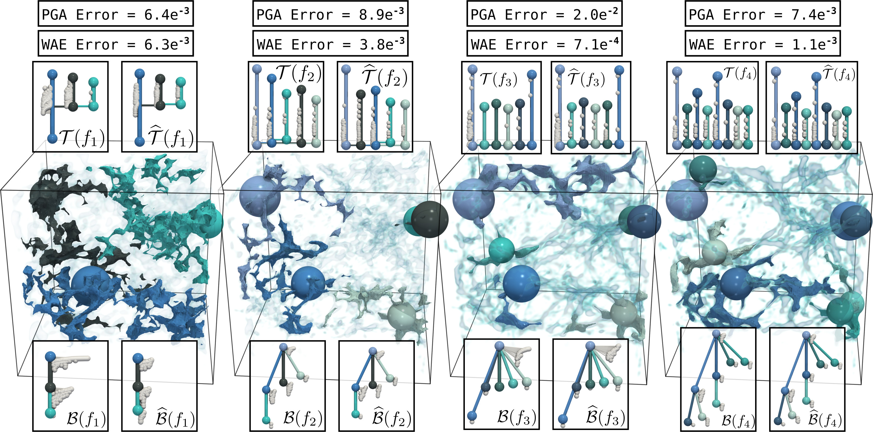
Figure 10: Application of our merge tree compression to topological clustering (experiment adapted from [pont_vis21, pont_tvcg23] for comparison purposes). The ensemble is clustered [pont_vis21] based on the merge trees (top left insets) of the ensemble members (each column represents a member from one of the $4$ clusters). The same clustering procedure [pont_vis21] is applied to the merge trees compressed by WAE (top right insets). Similarly to PGA [pont_tvcg23], the resulting clustering is identical with the compressed trees (it exactly matches the ground-truth classification [pont_vis21]). However, in comparison to PGA [pont_tvcg23], for a target compression factor of $15.09$, the relative reconstruction error (top) is clearly improved with WAE. Visually, the compressed trees look very similar to the original ones: the prominent features (in colors, non-prominent features are shown with small white nodes) are well preserved in terms of number and persistence. The same holds for the compressed BDTs (bottom right insets) which are nearly isomorphic to the original BDTs (bottom left insets, the color shows the assignment between the original and compressed BDTs).

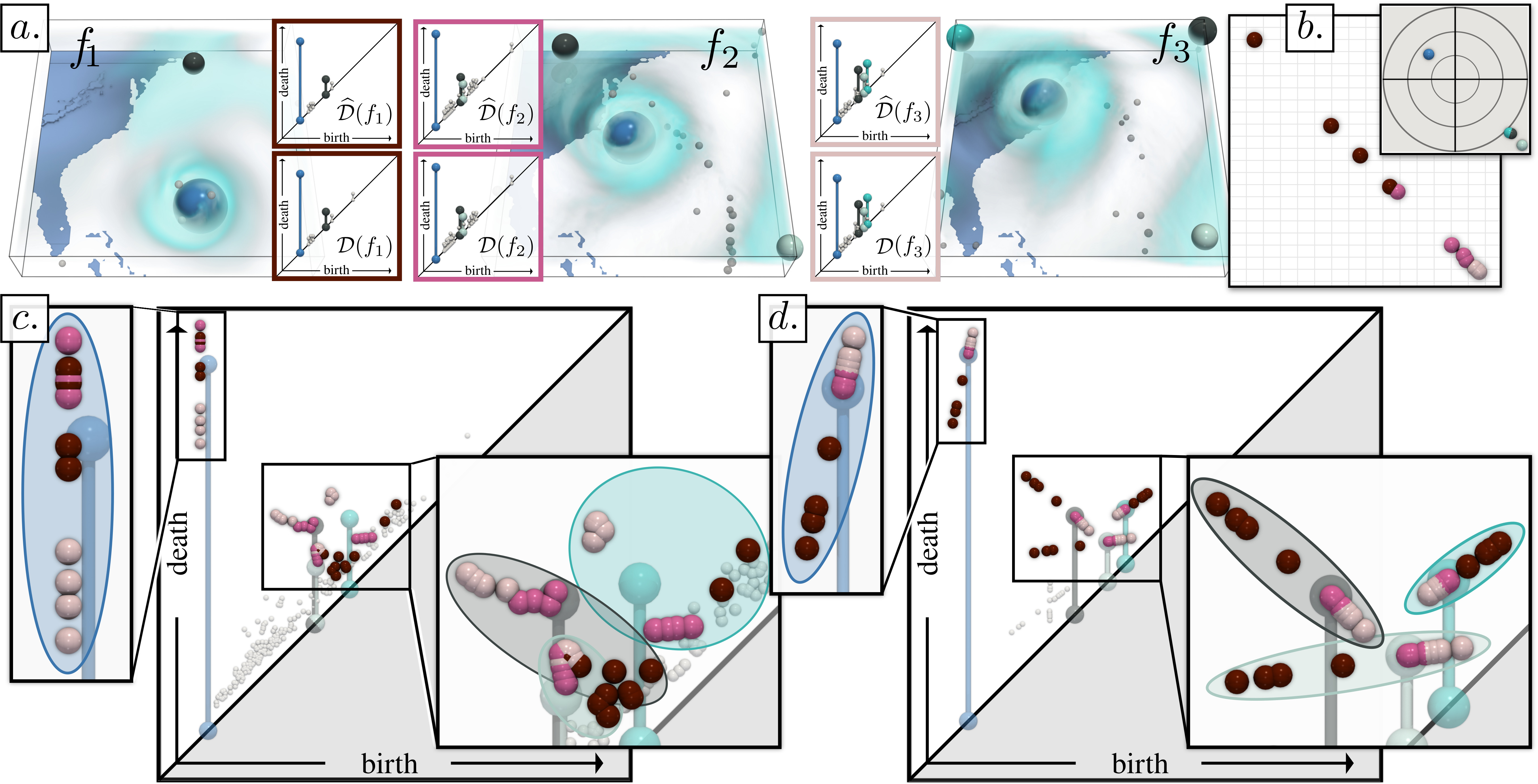
Figure 11: Visual analysis of the Isabel ensemble (one member per ground-truth class, top), with PD-WAE (in this example, $n_{e}=n_{d}=2$). Our work enables diagram compression, while providing reconstructed diagrams $\big{(}(a)$, top insets$\big{)}$ which are highly similar to the input (below). The 2D layout generated by PD-WAE $(b)$ recovers the temporal structure of the ensemble (the clusters are aligned in chronological order, from dark red to light pink). The PCV (grey inset) indicates that the peripheral gusts of wind in the data (white, black and cyan spheres) grow in importance when moving towards the bottom right corner of the latent space (their persistence increases over time). In contrast, the hurricane eye (light blue) exhibits less variability, but with stronger values towards the top left corner of the latent space (start of the sequence). The aggregated views (bottom, overlapping all diagrams, transparent: barycenter) for the input $(c)$ and the latent space $(d)$ show that PD-WAE nicely recovers a per-feature parameterization in the latent space (one ellipse per barycenter feature), which is locally consistent with the data temporal evolution (cluster color).

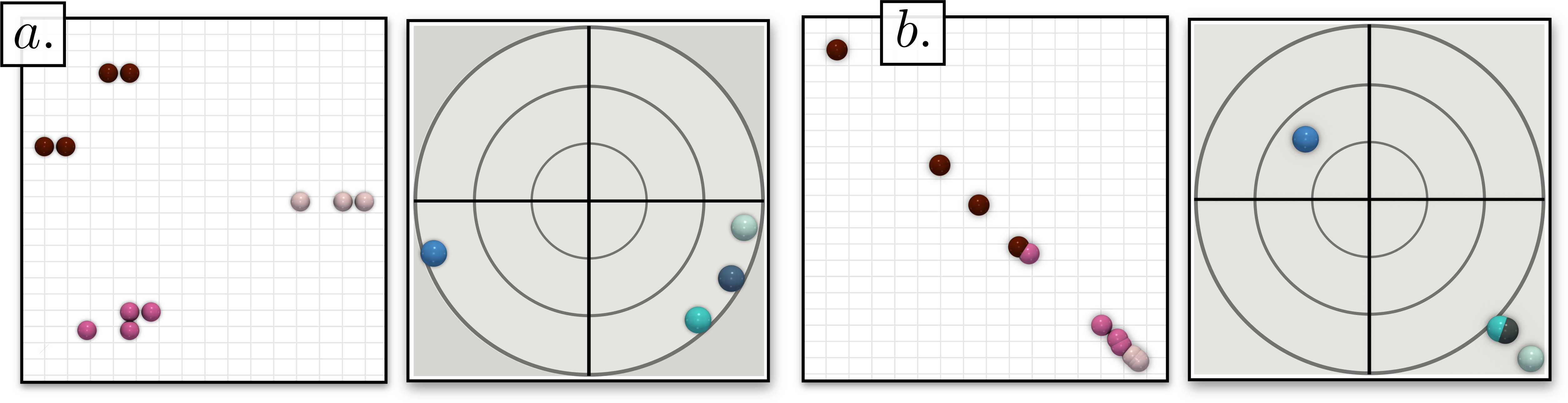
Figure 12: Qualitative comparison of the 2D layouts (left, white inset) and PCVs (right, grey inset) between PD-PGA [pont_tvcg23] (a) and PD-WAE (b) for the Isabel ensemble. PD-WAE manages to recover the intrinsic temporal structure of the ensemble and produces a linear alignment of the clusters in order of temporal appearance (dark red, pink, light pink).

Figs. 9 and 10 show two examples of visualization tasks (feature tracking and ensemble clustering, use cases replicated from [pont_vis21, pont_tvcg23] for comparison purposes). In these experiments, the BDTs have been compressed with the strategy described above. Next, the de-compressed BDTs have been used as an input to these two analysis pipelines. In both cases, the output obtained with the de-compressed BDTs is identical to the output obtained with the original BDTs. This shows the viability of the de-compressed BDTs and it demonstrates the utility of this compression scheme.

5.2 Dimensionality reduction

This section describes how to use MT-WAE to generate 2D layouts of the ensemble, for the global visual inspection of the ensemble. This is achieved by setting $d_{n_{e}}=2$ and by embedding each BDT $\mathcal{B}(f_{i})$ as a point in the plane, at its latent coordinates $(\alpha_{n_{e}}^{i})_{1}$ and $(\alpha_{n_{e}}^{i})_{2}$. This results in a summarization view of the ensemble, grouping similar BDTs together (Fig. 1c). The flexibility of our framework allows to further improve the quality of this 2D layout. Specifically, Appendix D introduces two penalty terms aiming at (1) improving the preservation of the Wasserstein metric $W^{\mathcal{T}}_{2}$ and (2) improving the preservation of the clusters of BDTs.

We augment our 2D layouts with Persistence Correlation Views (PCV) which were introduced in [pont_tvcg23]. In short, the PCV embeds a branch $b$ of the barycenter $\mathcal{B}_{*}$ [pont_vis21] as a point in 2D, in order to represent the variability of the corresponding feature in the ensemble, as a function of the coordinates in latent space. Specifically, the optimal assignments $\phi_{*_{i}}$ between $\mathcal{B}_{*}$ and each input BDT $\mathcal{B}(f_{i})$ is first computed (Eq. 1). Next, for a given branch $b\in\mathcal{B}_{*}$, the Pearson correlation $\rho\big{(}p_{b_{i}},(\alpha_{n_{e}}^{i})_{1}\big{)}$ between the persistence $p_{b_{i}}$ of $\phi_{*_{i}}(b)\in\mathcal{B}(f_{i})$ and the first coordinate in latent space $(\alpha_{n_{e}}^{i})_{1}$ is computed for the ensemble (i.e. for $i\in\{1,2,\dots,N\}$). Next, the Pearson correlation $\rho\big{(}p_{b_{i}},(\alpha_{n_{e}}^{i})_{2}\big{)}$ is computed similarly with regard to the second coordinate in latent space $(\alpha_{n_{e}}^{i})_{2}$. Finally, $b$ is embedded in the PCV at the coordinates $\Big{(}\rho\big{(}p_{b_{i}},(\alpha_{n_{e}}^{i})_{1}\big{)},\rho\big{(}p_{b_{i}},(\alpha_{n_{e}}^{i})_{2}\big{)}\Big{)}$. To avoid clutter in the visualization, we only report the most persistent branches of $\mathcal{B}_{*}$ in the PCV. Intuitively, points in the PCV which are located far away from the center, along a given direction, indicate a strong correlation between that direction in latent space, and the persistence of the corresponding feature in the ensemble.

PCVs enable the identification of patterns of feature variability within the ensemble, as discussed in Fig. 11. This case study considers the Isabel ensemble, which consists of $12$ scalar fields representing the wind velocity magnitude in a hurricane simulation. The ensemble comes with a ground-truth classification [pont_vis21]: $4$ members correspond to the formation of the hurricane (e.g. $f_{1}$, Fig. 11), $4$ other members to its drift (e.g. $f_{2}$, Fig. 11) and $4$ other members to its landfall (e.g. $f_{3}$, Fig. 11). For this ensemble, our PD-WAE approach produces a 2D layout $\big{(}$Fig. 11b)$\big{)}$ which manages to recover the temporal coherency of the ensemble: the formation (dark red), drift (pink) and landfall (light pink) clusters are arranged in order along a line $\big{(}$direction $(1,-1)\big{)}$. This shows the ability of PD-WAE to recover the intrinsic structure of the ensemble (here its temporal nature). The PCV (grey inset) further helps appreciate the variability of the features in the ensemble. There, each colored point indicates a persistent feature of the barycenter: the eye of the hurricane is represented by the blue sphere, while the cyan, black and white sphere represent peripheral gusts of wind $\big{(}$see the matching features in the data, Fig. 11a)$\big{)}$. The PCV clearly identifies two patterns of feature variability, along the direction $(1,-1)$, which coincides with the temporal alignment of the clusters in latent space. Specifically, it indicates that the persistence of the hurricane eye will be larger in the top left corner of the latent space, i.e. towards the beginning of the temporal sequence (dark red cluster). This is confirmed visually when inspecting the persistence diagrams of the individual members (the blue feature is less persistent in $\mathcal{D}(f_{3})$ than in $\mathcal{D}(f_{1})$ and $\mathcal{D}(f_{2})$). In short, this visually encodes the fact that the strength of the hurricane eye decreases with time. In contrast, the features corresponding to peripheral wind gusts (cyan, black and white spheres) exhibit a common variability pattern, distinct form that of the hurricane eye: the persistence of the corresponding features increases as one moves along the direction $(1,-1)$ in latent space, i.e. as time increases (pink and light pink clusters). This is confirmed visually in the individual members, where the persistence of these features is larger in $\mathcal{D}(f_{3})$ than in $\mathcal{D}(f_{1})$ and $\mathcal{D}(f_{2})$. In short, this visually encodes the fact that the strength of the peripheral wind gusts increases with time. Overall, while the 2D layout generated by PD-WAE enables the visualization of the intrinsic structure of the ensemble (here, its temporal nature), the PCV enables the visualization and interpretation of the variability in the ensemble at a feature level. The caption of Fig. 1 includes a similar discussion for MT-WAE.

Fig. 12 provides a qualitative comparison of the 2D layouts and Persistence Correlation Views (PCVs) between PD-PGA [pont_tvcg23] and our novel non-linear framework, PD-WAE (see Sec. 6.2 for an extensive quantitative comparison). Specifically, it shows that, while PD-PGA $\big{(}$Fig. 12a)$\big{)}$ manages to isolate the clusters well, its 2D layout does not recover the intrinsic, one-dimensional, temporal structure of the ensemble. In contrast, as discussed above, PD-WAE $\big{(}$Fig. 12b)$\big{)}$ manages to recover this intrinsic structure and produces a linear alignment of the clusters along the direction $(1,-1)$, in order of their temporal appearance. This alignment greatly facilitates the interpretation of the PCV, since time is now visually encoded there by the linear direction $(1,-1)\big{)}$ (whereas it would be encoded by a curve in the case of PD-PGA).

In contrast to standard auto-encoders, our approach explicitly manipulates topological descriptors throughout the network. This results in improved interpretability and enables new capabilities:

(1) Latent feature transformation: As discussed in Fig. 11, it is now possible to visualize how topological descriptors are (non-linearly) transformed by the auto-encoder. Specifically, the aggregated views of the birth/death space (bottom) illustrates how PD-WAE unwraps the diagrams in latent space, nicely recovering the data temporal evolution at a feature level (see the temporally consistent linear arrangements of points for each barycenter feature in Fig. 11d), from dark red to pink and light pink).

(2) Latent space navigation: Given a point in latent space, it is now possible to efficiently reconstruct its BDT/MT by propagating its latent coordinates through the decoding layers, enabling an interactive exploration of the merge tree latent space (Fig. 1d).

(3) Feature traversal analysis: For each consecutive layers $\Pi_{k}$ and $\Pi_{k+1}$, we compute the optimal assignment (Eq. 1) between their input origins, $\mathcal{O}_{k}^{in}$ and $\mathcal{O}_{k+1}^{in}$. Next, we compute the optimal assignment between the barycenter $\mathcal{B}_{*}$ [pont_vis21] of the input ensemble and the first origin $\mathcal{O}_{1}^{in}$. This yields an explicit tracking of each branch $b$ of $\mathcal{B}_{*}$ down to the latent space. We introduce the notion of Feature Latent Importance (FLI), given by the persistence of $b$ in latent space, divided by its original persistence. FLI indicates if a feature gains (or looses) importance in latent space. This enables the identification of the most informative features in the ensemble.

This is illustrated in Fig. 1e), where the cyan, white, dark blue and black features exhibit large FLI values (red circles). In the trees, these features are indeed present in most of the ensemble $\big{(}$Fig. 1d)$\big{)}$, with only moderate variations in persistence. Interestingly, the global maximum of seismic wave (light blue feature) is not a very informative feature (light blue circle): while it is also present throughout the sequence, its persistence decreases significantly (left to right). This visually encodes that, as the seismic wave travels from the epicenter, the strength of its global maximum is no longer significant in front of other local maxima (which illustrates the energy diffusion process).

Table 1: Running times (in seconds) of our algorithm for PD-WAE and MT-WAE computation (first sequential, then with 20 cores).

Dataset	$N$	$|\mathcal{B}|$	PD-WAE			MT-WAE
			1 c.	20 c.	Speedup	1 c.	20 c.	Speedup
Asteroid Impact (3D)	7	1,295	2,819.38	989.42	2.85	5,946.81	1,522.89	3.90
Cloud processes (2D)	12	1,209	11,043.20	1,318.63	8.37	16,150.90	2,566.98	6.29
Viscous fingering (3D)	15	118	1,345.31	268.78	5.01	3,727.64	417.31	8.93
Dark matter (3D)	40	316	125,724.00	10,141.30	12.40	135,962.00	8,051.02	16.89
Volcanic eruptions (2D)	12	811	4,925.15	638.58	7.71	4,151.04	449.14	9.24
Ionization front (2D)	16	135	627.04	95.31	6.58	1,140.44	144.57	7.89
Ionization front (3D)	16	763	17,285.10	1,757.71	9.83	101,788.00	5,350.46	19.02
Earthquake (3D)	12	1,203	14,272.10	2,074.52	6.88	9,888.68	1,024.45	9.65
Isabel (3D)	12	1,338	3,485.03	436.56	7.98	23,240.90	1,669.20	13.92
Starting Vortex (2D)	12	124	215.46	95.45	2.26	281.80	147.51	1.91
Sea Surface Height (2D)	48	1,787	41,854.70	2,901.39	14.43	222,594.00	13,540.20	16.44
Vortex Street (2D)	45	23	460.46	152.35	3.02	117.88	38.88	3.03

6 Results

This section presents experimental results obtained on a computer with two Xeon CPUs (3.2 GHz, 2x10 cores, 96GB of RAM). The input merge trees were computed with FTM [gueunet_tpds19] and pre-processed to discard noisy features (persistence simplification threshold: $0.25\%$ of the data range). We implemented our approach in C++ (with OpenMP and PyTorch’s C++ API [pytorch]), as modules for TTK [ttk17, ttk19]. Experiments were performed on a set of $12$ public ensembles described in [pont_vis21], which includes a variety of simulated and acquired 2D and 3D ensembles extracted from previous work and past SciVis contests [scivisOverall].

6.1 Time performance

The Wasserstein distance computation (Eq. 1) is the most expensive sub-procedure of our approach. It intervenes during energy evaluation (Sec. 4.5) but also at each iteration of basis projection (Sec. 4.2), itself occuring at each propagation iteration (Sec. 4.4), for each input BDT. To compute this distance, we use a fine-grain task-based parallel algorithm [pont_vis21]. We leverage further parallelism to accelerate the process. Specifically, for each input BDT, its forward propagation (Sec. 4.4) can be run in a distinct parallel task. Similarly, when evaluating the overall energy (Sec. 4.5), the distance between an input BDT and its output reconstruction is computed in a distinct parallel task for each BDT. Tab. 1 evaluates the time performance of our framework for persistence diagrams (PD-WAE) and merge trees (MT-WAE). In sequential mode, the computation time is a function of the ensemble size ($N$), the tree sizes ($|\mathcal{B}|$), and the network size ($n_{e}+n_{d}$). Specifically, our approach computes, for each optimization iteration, $n_{it}\times(n_{e}+n_{d})\times N$ Wasserstein distances, each of which requiring $\mathcal{O}(|\mathcal{B}|^{2})$ steps in practice. In parallel, the iterative nature of our approach (Alg. 1) challenges parallel efficiency. However, timings are still improved after parallelization (orders of minutes on average), with a very good parallel efficiency for the largest ensembles (up to 95%).

6.2 Framework quality

Figs. 9 and 10 report compression factors for our application to merge tree compression (Sec. 5.1). These are ratios between the storage size of the input $N$ BDTs and that of their compressed form. For a fixed target compression factor, WAE clearly improves the reconstruction error over linear encoding (PGA [pont_tvcg23]). Appendix E extends this error comparison to all our test ensembles, and shows that, for identical compression factors, our framework improves the reconstruction error over PGA [pont_tvcg23] by 37% for persistence diagrams, and 52% for merge trees, hence confirming the accuracy superiority of WAE over PGA.

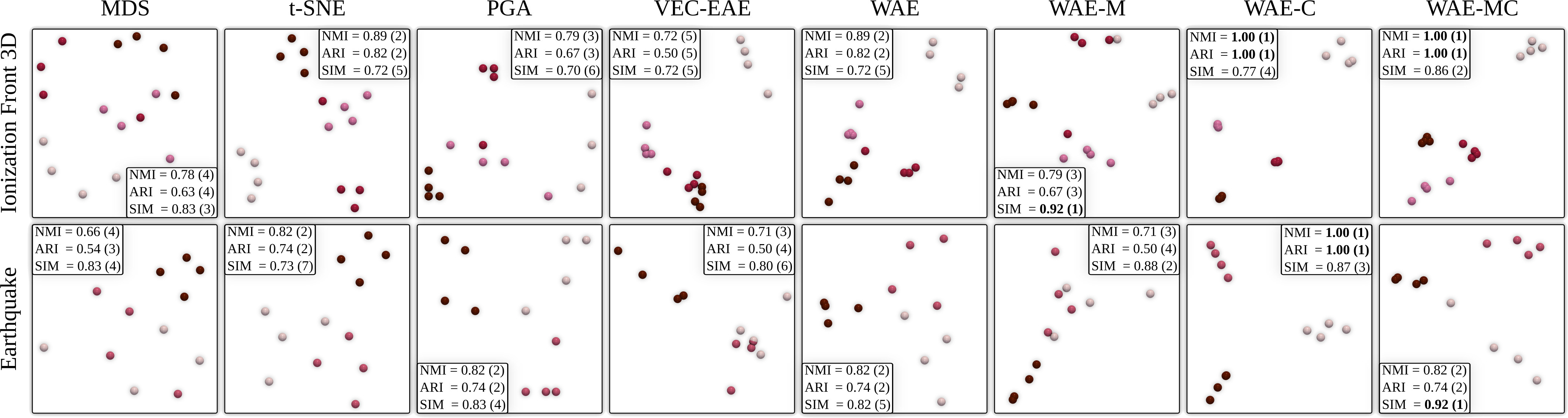
Figure 13: Comparison of planar layouts for typical dimensionality reduction techniques, on two merge tree ensembles. The color encodes the classification ground-truth [pont_vis21]. For each quality score, the best value appears bold and the rank of the score is shown in parenthesis. This experimental protocol is adapted from [pont_tvcg23] for comparison purposes.

Fig. 13 provides a visual comparison for the planar layouts generated by a selection of typical dimensionality reduction techniques, applied on the input merge tree ensemble (i.e. each point is a merge tree). This experiment is adapted from [pont_tvcg23] for comparison purposes. This figure reports quantitative scores. For a given technique, to quantify its ability to preserve the structure of the ensemble (i.e. its organization into ground-truth classes), we run $k$-means in the 2D layouts and evaluate the quality of the resulting clustering (given the ground-truth [pont_vis21]) with the normalized mutual information (NMI) and adjusted rand index (ARI). To quantify its ability to preserve the geometry of the ensemble (i.e. to preserve its disposition within the Wasserstein metric space $\mathbb{B}$), we report the metric similarity indicator SIM [pont_tvcg23], which evaluates the preservation of the Wasserstein metric $W^{\mathcal{T}}_{2}$. All these scores vary between $0$ and $1$, with $1$ being optimal.

MDS [kruskal78] and t-SNE [tSNE] have been applied on the distance matrix of the input merge trees (Wasserstein distance, Eq. 1, default parameters [pont_vis21]). By design, MDS preserves well the metric $W^{\mathcal{T}}_{2}$ (good SIM), at the expense of mixing ground-truth classes together (low NMI/ARI). t-SNE behaves symmetrically (higher NMI/ARI, lower SIM). We applied PGA [pont_tvcg23] by setting the origin size parameter to a value compatible to our latent space ($0.1|\mathcal{S}_{\mathcal{B}}|$, Appendix C). As expected, PGA provides a trade-off between the extreme behaviors of MDS and t-SNE, with an improved cluster preservation over MDS (NMI/ARI), and an improved metric preservation over t-SNE (SIM). WAE also constitutes a trade-off between MDS and t-SNE, but with improved quality scores over PGA.

Table 2: Comparison of aggregated layout quality scores (i.e. averaged over all merge tree ensembles, bold: best values). WAE-MC provides both superior metric (SIM) and cluster (NMI/ARI) preservation to pre-existing techniques (MDS [kruskal78], t-SNE [tSNE], PGA [pont_tvcg23], VEC-EAE).

Indicator	MDS	t-SNE	PGA	VEC-EAE	WAE	WAE-M	WAE-C	WAE-MC
NMI	0.78	0.83	0.82	0.71	0.84	0.76	0.96	0.87
ARI	0.68	0.75	0.74	0.55	0.77	0.63	0.95	0.82
SIM	0.86	0.75	0.79	0.74	0.78	0.87	0.78	0.86

We compare our approach to a standard auto-encoder (EAE, Sec. 3.1) applied on the following vectorization of the input merge trees. Note that several vectorizations of persistence diagrams have been studied [Adams2015, Bubenik15, kim20]. However we focus in this work on merge trees and only few vectorizations have been documented for these [LI2021]. Hence we focus on the following strategy, inspired by [LI2021]. Each input BDT $\mathcal{B}(f_{i})$ is embedded in $\mathbb{R}^{2|\mathcal{B}_{*}|}$, such that the $j^{th}$ entry of this vector corresponds to the birth/death location of the branch of $\mathcal{B}(f_{i})$ which maps to the $j^{th}$ branch of the barycenter $\mathcal{B}_{*}$ [pont_vis21]. Next, we feed these vectorizations to an EAE, with the same meta-parameters as our approach (i.e. number of layers, dimensionality per layer). The corresponding results appear in the VEC-EAE column. Our approach (WAE) outperforms this straightforward application of EAE, with clearly higher clustering scores (NMI/ARI) and improved metric scores (SIM).

Fig. 13 also reports the layouts obtained with our approach after enabling the metric penalty term (WAE-M), the clustering penalty term (WAE-C) and both (WAE-MC), c.f. Appendix D. WAE-M (respectively WAE-C) significantly improves the metric (respectively cluster) preservation over MDS (repectively t-SNE). The combination of the two terms (WAE-MC) improves both quality scores simultaneously: it outperforms MDS (SIM) and it improves t-SNE (NMI/ARI). In other words, WAE-MC improves established methods by outperforming them on their dedicated criterion (SIM for MDS, NMI/ARI for t-SNE).

Appendix F extends our visual analysis to all our test ensembles. Tab. 2 also extends our quantitative analysis to all our test ensembles. It confirms the clear superiority of WAE over VEC-EAE. It also confirms that the combination of our penalty terms (WAE-MC) provides the best metric (SIM) and cluster (NMI/ARI) scores over existing techniques.

6.3 Limitations

As discussed in Sec. 2.2, the parameter $\epsilon_{1}$ of the Wasserstein distance between merge trees ($W^{\mathcal{T}}_{2}$) acts as a control knob, that balances the practical stability of the metric with its discriminative power. Specifically, for $\epsilon_{1}=1$, we have $W^{\mathcal{T}}_{2}=W^{\mathcal{D}}_{2}$ and $W^{\mathcal{T}}_{2}$ is stable, but less discriminative. Pont et al. [pont_vis21] showed experimentally that for relatively low values of $\epsilon_{1}$ ($0.05$), $W^{\mathcal{T}}_{2}$ still behaved in a stable manner in practice for reasonable noise levels. Our overall MT-WAE framework behaves similarly. Appendix G provides a detailed empirical stability evaluation of our framework in the presence of additive noise. In particular, this experiment shows that for reasonable levels of additive noise $\epsilon$ (normalized with regard to the function range), typically $\epsilon<0.1$, the recommended default value of $\epsilon_{1}$ ($0.05$) results in a stable MT-WAE computation. For larger noise levels ($\epsilon>0.1$), MT-WAE provides similar stability scores to PD-WAE, for values of $\epsilon_{1}$ which are still reasonable in terms of discriminative power ($\epsilon_{1}=0.1$).

A possible direction to improve the practical stability of the framework without having to deal with a control parameter such as $\epsilon_{1}$ would be to consider branch decompositions driven by other criteria than persistence (such as hyper-volume [carr04] for instance). However, the persistence criterion plays a central role in the Wasserstein distance between merge trees, as discussed by Pont et al. [pont_vis21] (Sec. 4), in particular to guarantee that interpolated BDTs computed during geodesic construction can indeed be inverted into a valid MT. Thus, other branch decomposition criteria than persistence would require to derive a completely new procedure for several key components of our framework, such as geodesic computation or barycenter estimation. This is an orthogonal research direction to this work, which we leave for future work.

Similarly to other optimization problems based on topological descriptors [Turner2014, vidal_vis19, pont_vis21, pont_tvcg23], our energy is not convex. However, our experiments indicate that our initialization strategy (Sec. 4.3) leads to relevant solutions, which can be successfully applied for visualization (Sec. 5).

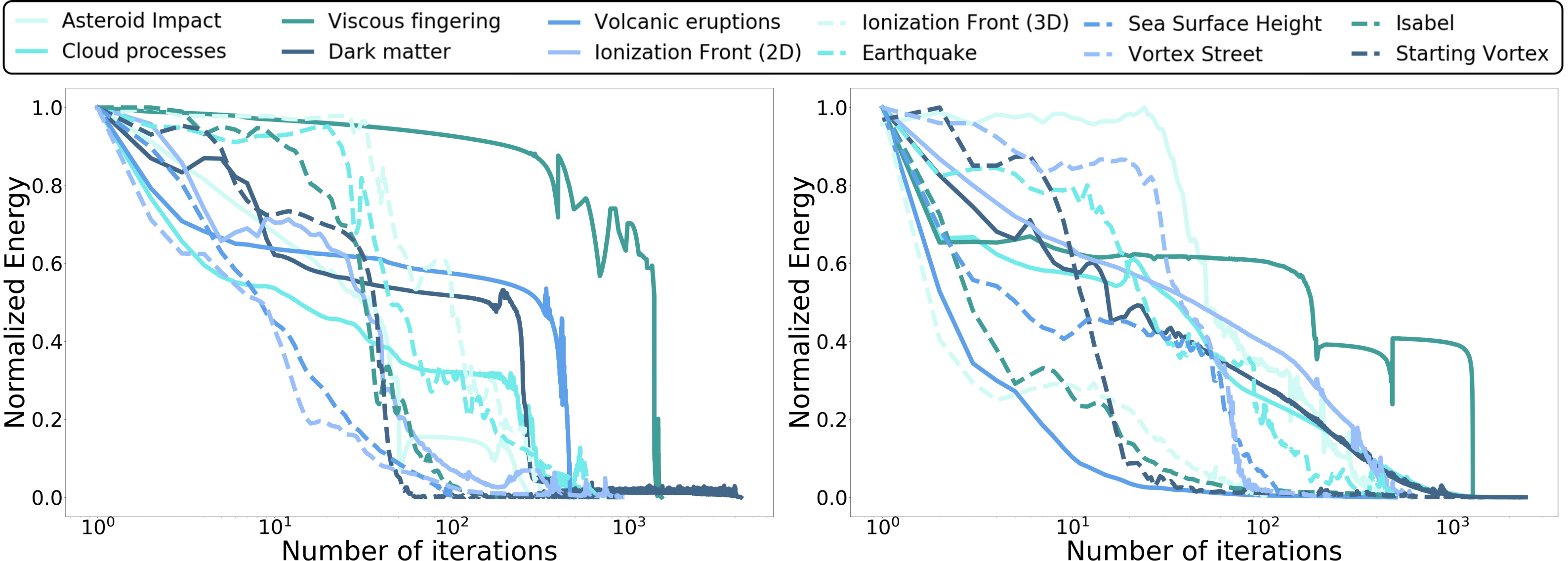
Figure 14: Evolution of the normalized reconstruction error along the iterations, for PD-WAE (left) and MT-WAE (right).

Since it is based on neural networks, our approach inherits from their intrinsic limitations. Specifically, the energy is not guaranteed to monotonically decrease over the iterations. However, this theoretical limitation has never translated into a practical limitation in our experiments. Fig. 14 reports the evolution of the normalized reconstruction error for PD and MT-WAE computations, for all our test ensembles. In particular, it shows that typical, temporary energy increases can indeed be observed (as often reported when optimizing neural networks), but without preventing the network from converging overall (i.e. reaching a state where the energy decreases by less than $1\%$ between consecutive iterations). Like other neural methods, our approach is conditioned by the meta-parameters defining the network (i.e. number of layers, dimensionality of each layer, etc.). However, we ran our experiments with fairly basic values for these meta-parameters (as detailed in Appendix C) and still obtained substantial improvements over linear encoding based on PGA [pont_tvcg23]. This indicates that optimizing in the future these meta-parameters is likely to improve the quality of our framework, however possibly at the expense of longer computations. Finally, our application to merge tree compression does not guarantee any error bound in its current form, which we leave for future work.

7 Conclusion

In this paper, we presented a computational framework for the Wasserstein Auto-Encoding of merge trees (and persistence diagrams), with applications to merge tree compression and dimensionality reduction. Our approach improves previous linear attempts at merge tree encoding, by generalizing them to non-linear encoding, hence leading to lower reconstruction errors. In contrast to traditional auto-encoders, our novel layer model enables our neural networks to process topological descriptors natively, without pre-vectorization. As shown in our experiments, this contribution leads not only to superior accuracy (Sec. 6.2) but also to superior interpretability (Sec. 5.2): with our work, it is now possible to interactively explore the latent space and analyze how topological features are transformed by the network in its attempt to best encode the ensemble. Overall, the visualizations derived from our contribution (Figs. 1, 11) enable the interactive, visual inspection of the ensemble, both at a global level (with our 2D layouts) and at a feature level. Specifically, our novel notion of feature latent importance enables the identification of the most informative features in the ensemble.

In the future, we will continue our work towards the development of further statistical tools for the visual analysis of ensemble data, based on topological descriptors. In particular, there are several research avenues for improving our current approach. For example, the Wasserstein distance between merge trees is subject to several meta-parameters (Sec. 2.2), for which we provide generic default values which have shown to be relevant in practice. A possible improvement could consist in letting the auto-encoding framework optimize these meta-parameters (on a per branch basis). However, this data-driven setup of the meta-parameters of our approach would come at the expense of extended running times. Another research avenue could consist in combining our framework with existing approaches on topological losses for image segmentation [HuLSC19, HuWLSC21, StuckiPSMB23], in order to also auto-encode the scalar data. Moreover, another direction could consist in training a single neural network for auto-encoding multiple ensembles at once. However, this would require to derive new normalization strategies, since, as the scalar fields can take arbitrarily distinct value ranges from an ensemble to the next, the Wasserstein distances between their members can also take arbitrarily distinct values, which would challenge an efficient sampling of the metric space. Finally, we will investigate the usage of neural networks exploiting topological descriptors for further visual analysis tasks, such as trend analysis or anomaly detection or shape classification [shrec14]. In that context, we believe that our new layer model (natively processing topological descriptors) sets the foundations for an accurate and interpretable usage of topological representations with neural networks.