Non-equilibrium steady state of the symmetric exclusion process with reservoirs

Abstract.

Consider the open symmetric exclusion process on a connected graph with vertexes in $[N-1]:=\{1,\ldots,N-1\}$ where points $1$ and $N-1$ are connected, respectively, to a left reservoir and a right reservoir with densities $\rho_{L},\rho_{R}\in(0,1)$. We prove that the non-equilibrium steady state of such system is

$$\mu_{\rm{stat}}=\sum_{I\subset\mathcal{P}([N-1])}F(I)\bigg{(}\otimes_{x\in I}\rm{Bernoulli}(\rho_{R})\otimes_{y\in[N-1]\setminus I}\rm{Bernoulli}(\rho_{L})\bigg{)}.$$

In the formula above $\mathcal{P}([N-1])$ denotes the power set of $[N-1]$ while the numbers $F(I)>0$ are such that $\sum_{I\subset\mathcal{P}([N-1])}F(I)=1$ and given in terms of absorption probabilities of the absorbing stochastic dual process. Via probabilistic arguments we compute explicitly the factors $F(I)$ when the graph is a homogeneous segment.

1. introduction

1.1. Boundary driven systems

In the context of non-equilibrium statistical physics, a lot of attention has been devoted to the study of stationary properties of open particle systems evolving on a finite graph (see, e.g., [4] and [26] for an overview on the subject). The word open refers to the fact that the dynamics does not conserve the total number of particles due to an interaction with the external world, typically modelled via particle reservoirs (see, e.g., [10] and [6] ) or, in heat transfer, via thermal baths (see, e.g., [22] and [18]): such systems are thus referred to as boundary driven. Reservoirs are mechanisms that inject and remove particles from the system, imposing a fix density of particles at a given site of the graph. When multiple reservoirs, each imposing different density values, are connected to the graph, the system is considered to be out of equilibrium. This condition is characterized by the presence of a non-zero particle current at stationarity, and the stationary measure of the system is commonly referred to as the non-equilibrium steady state. While for many closed (as opposite of open) particle systems, the stationary, actually reversible, measures are explicit and in product form, the action of the reservoirs destroy reversibility and long range correlations can emerge in the non-equilibrium steady state as shown in the seminal paper [31]. Finding explicit stationary measures for open systems is a key problem in statistical physics, and it continues to generate substantial interest (see, e.g., the recent works [14], [16] and [15]).

For some systems, the celebrated matrix product ansatz method has been developed in [10] to obtain in explicit form such long range correlations. This method works, for instance, for the open simple symmetric exclusion process (SSEP) on a one dimensional segment with sites $\{1,\ldots,N-1\}$ where points $\{1,N-1\}$ are connected, respectively, to a left and a right reservoir. This is a system of simple symmetric random walks subject to the exclusion rule: only one particle per site is allowed and thus attempted jumps to occupied sites are suppressed. Moreover at sites $\{1,N-1\}$ particles are destroyed and created at specific given rates. After [10], other matrix and algebraic methods have been proposed to compute explicitly the correlations of the open SSEP (see [29], [24] and [15]) and the research around this system is extremely active (see, e.g., [28, 17, 20, 5, 23, 11]).

However, a probabilistic representation of the non-equilibrium steady state of the open SSEP complementing the explicit correlations computed via the matrix ansatz is still not available in the literature and the matrix computations performed in e.g. [10] lack a probabilistic interpretation.

Moreover, matrix ansatz methods strongly rely on the fact that the underlying graph is a homogeneous segment and particles perform nearest neighbor jumps, while there are several natural reasons why one would like to overcome such limitation. First, many physical systems are not one dimensional and modelling the open SEP on a graph approximating a $d$-dimensional domain started to receive attention recently (see [8]). Second, realistic models of particles should take care of the presence of spatial inhomogeneities (see, e.g., [27]) in the underlying media and these are often modelled with edge dependent weights. Third, extensive research has been conducted on the effects of symmetric long-range jumps in open exclusion processes, revealing interesting phenomena (see, e.g., [2], [1], [21] and [3]).

The boundary driven symmetric exclusion process (SEP) on a general graph satisfies a property that turns out to be extremely useful: it is in stochastic duality relation with a dual particle system where particles evolve as in the primal model but the reservoirs are replaced by absorbing sites (see, e.g., [6] and the recent work [30]). Thus the dual system is conservative and if the graph is connected, all the particles will be eventually absorbed. More precisely, this relation allow to compute the expected evolution of products of occupation variables of $n$ sites via the dual absorbing process with $n$ particles only.

In this paper we will use this relation to show that on a general graph with symmetric weights, the non-equilibrium steady state of the open SEP is a mixture measure of product of Bernoulli measures. Moreover we develop a probabilistic approach to derive the explicit formulas previously achieved by the matrix product ansatz and other algebraic methods.

1.2. Boundary driven SEP and its stationary distribution

Let $G$ be a finite connected graph with vertex set $[N-1]:=\{1,\ldots,N-1\}$ and edge set $E$. To each edge $\{x,y\}\in E$ we associate a symmetric weight $\omega_{x,y}\in(0,\infty)$ called conductance. We thus identify $G$ with the triple $([N-1],E,(\omega_{x,y})_{\{x,y\}\in E})$. The boundary driven SEP on $G$ with reservoirs parameters $\rho_{L},\rho_{R}\in(0,1)$ and $\omega_{L},\omega_{R}>0$ is the Markov process $(\eta_{t})_{t\geq 0}$ with state space $\mathcal{X}=\{0,1\}^{[N-1]}$ and infinitesimal generator

$${\mathcal{L}}={\mathcal{L}}+\omega_{L}\,{\mathcal{L}}_{L}+\omega_{R}\,{\mathcal{L}}_{R}$$ (1.1)

where, for all bounded functions $f:{\mathcal{X}}\to{\mathbb{R}}$,

$${\mathcal{L}}^{\text{bulk}}f(\eta)=\ \sum_{\{x,y\}\in E}\omega_{x,y}\left\{\begin{array}[]{c}\eta(x)\,(1-\eta(y))\left(f(\eta^{x,y})-f(\eta)\right)\\[4.26773pt] +\,\eta(y)\,(1-\eta(x))\left(f(\eta^{y,x})-f(\eta)\right)\end{array}\right\}\ ,$$

$$\mathcal{L}_{L}f(\eta)= \ \eta(1)\,(1-\rho_{L})\,(f(\eta^{1,-})-f(\eta))$$

$$+ \ \rho_{L}\,(1-\eta(1))\,(f(\eta^{1,+})-f(\eta))$$

and

$$\mathcal{L}_{R}f(\eta)= \ \eta(N-1)\,(1-\rho_{R})\left(f(\eta^{N-1,-})-f(\eta)\right)$$

$$+ \ \rho_{R}\left(1-\eta(N-1))\,(f(\eta^{N-1,+})-f(\eta)\right)\ .$$

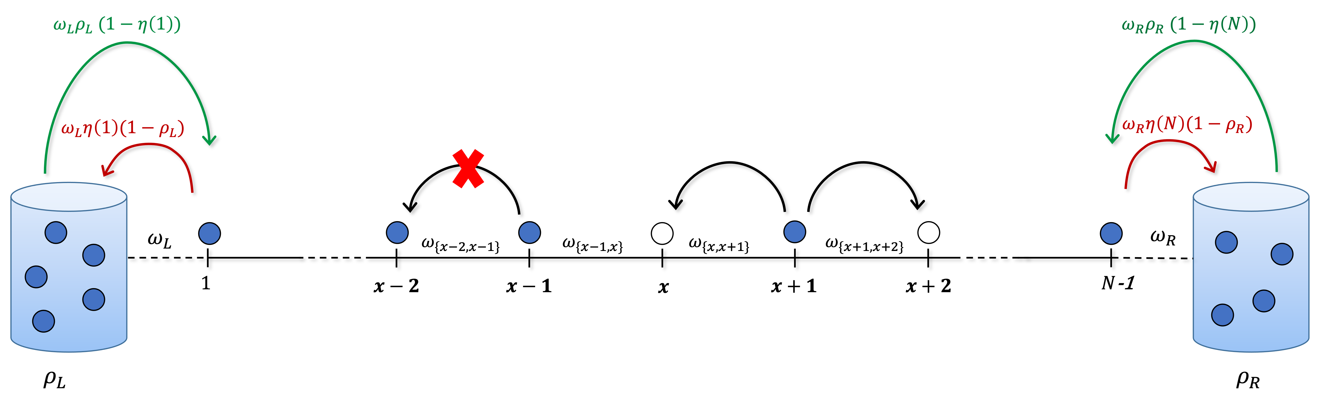
Figure 1. Schematic description of the dynamics.

Above $\eta^{x,y}$ is the configuration in which a particle (if any) has been removed from $x\in[N-1]$ and moved at $y\in[N-1]$, while $\eta^{x,-}\in\mathcal{X}$ is the configuration obtained from $\eta$ by destroying a particle (if present) from site $x\in\{1,N-1\}$ and $\eta^{x,+}\in\mathcal{X}$ is the configuration obtained from $\eta$ by creating a particle (if not already present) at site $x\in\{1,N-1\}$. In the above dynamics, the action of the reservoirs corresponds to the $\omega_{L}\,{\mathcal{L}}_{L}+\omega_{R}\,{\mathcal{L}}_{R}$ part of the generator. $\rho_{L}$ is the particle density imposed by the left reservoir and $\rho_{R}$ the one imposed by the right reservoir. $\omega_{L}$ is the conductance connecting the site $1$ to the fictitious point $0$ representing the left reservoir and $\omega_{R}$ is the conductance connecting the site $N-1$ to the fictitious point $N$ representing the right reservoirs.

It is well known that $(\eta_{t})_{t\geq 0}$ is in stochastic duality relation with the Markovian interacting particle system $(\xi_{t})_{t\geq 0}$ with state space $\mathcal{X}\times{\mathbb{N}}_{0}^{\{0,N\}}$ and which evolves as the SEP on $G$ but the reservoirs are now replaced by absorbing sites $\{0,N\}$. More precisely, in the dual system a particle at site $1$ can be absorbed at site $0$ at rate $\omega_{L}$ and a particle at site $N-1$ can be absorbed at site $N$ at rate $\omega_{R}$. We denote by $\hat{\mathbb{P}}_{\xi}$ the law of $(\xi_{t})_{t\geq 0}$ starting from the configuration $\xi$ which can be identified with a subset $I$ of vertexes in $[N-1]\cup\{0,N\}$ via the relation $\xi(x)=\boldsymbol{1}_{\{x\in I\}}$. Thus we write either $\hat{\mathbb{P}}_{\xi}$ or $\hat{\mathbb{P}}_{I}$. We refer the reader to Section 2.1 below for the precise definition of $(\xi_{t})_{t\geq 0}$ and for the duality relation satisfied by the two processes.

Our first main contribution is the following theorem. We denote by $\mathcal{P}([N-1])$ the power set of $[N-1]$ and given $I\in\mathcal{P}([N-1])$, $|I|$ denotes its cardinality.

Theorem 1.1.

The stationary distribution of the boundary driven SEP on $G$ with reservoirs parameters $\rho_{L},\rho_{R},\omega_{L},\omega_{R}>0$ is

$$\mu_{\rm{stat}}=\sum_{I\subset\mathcal{P}([N-1])}F(I)\bigg{(}\otimes_{x\in I}\rm{Bernoulli}(\rho_{R})\otimes_{y\in[N-1]\setminus I}\rm{Bernoulli}(\rho_{L})\bigg{)},$$ (1.2)

where

$$F(I):=\sum_{J\subset\mathcal{P}([N-1]):\ I\subset J}(-1)^{|J\setminus I|}\hat{\mathbb{P}}_{J}(\xi_{\infty}(N)=|J|)>0$$ (1.3)

satisfies

$$\sum_{I\subset\mathcal{P}([N-1])}F(I)=1.$$

Remark 1.2 (Probabilistic interpretation of $F(I)$).

As it will be clear from Theorem 2.2 below, each factor $F(I)$ is the probability that all the particles initially at $I$ are absorbed at $N$, while the remaining ones at $0$, in the dual system of the boundary driven SEP, built via the labelled stirring construction and started from particles in each site of the bulk $[N-1]$.

Remark 1.3.

From (1.2) one can deduce that for all $\eta\in\mathcal{X}$,

$$\mu_{\rm{stat}}(\eta)=\sum_{\ell=0}^{|\eta|}\sum_{k=0}^{N-1-|\eta|}\rho_{R}^{\ell}\rho_{L}^{|\eta|-\ell}(1-\rho_{R})^{k}(1-\rho_{L})^{N-1-|\eta|-k}\left(\sum_{I\in C(\ell,k)}F(I)\right)$$

where $C(\ell,k)=\{I\in\mathcal{P}([N-1]):|I|=k+\ell\ \rm{and}\ |I\cap\eta|=\ell\}$.

1.3. Explicit formulas for boundary driven SEP

Providing explicitly the factors $F(I)$ amounts to compute the absorption probabilities in the dual system: via a coupling technique we compute such probabilities when the graph is a homogeneous one dimensional segment.

Theorem 1.4.

If  $\omega_{x,y}={{\bf 1}}_{\{|x-y|=1\}}$ for each $x,y\in[N-1]$ and $\omega_{L}=\omega_{R}=1$, then, given $1\leq x_{1}<\ldots<x_{n}\leq N-1$,

$$\hat{\mathbb{P}}_{\{x_{1},\ldots,x_{n}\}}(\xi_{\infty}(N)=n)=\prod_{i=1}^{n}\frac{x_{i}-(i-1)}{N-(i-1)}.$$ (1.4)

In several works (see, e.g., [17, 20]) the following choice of parameters is taken

$$\begin{split}\rho_{L}=\frac{\alpha}{\alpha+\gamma}\\ \rho_{L}=\frac{\delta}{\delta+\beta}\end{split}\begin{split}\omega_{L}=&\frac{1}{\alpha+\gamma}\\ \omega_{R}=&\frac{1}{\delta+\beta}\end{split}$$

obtaining the $\alpha,\beta,\gamma,\delta$ model where particles are created at rate $\alpha$ on the left and at rate $\delta$ on the right while particles are destroyed at rate $\gamma$ on the left and $\beta$ on the right. In the setting of Theorem 1.4 but with general values of $\omega_{L}$ and $\omega_{R}$ as in the $\alpha,\beta,\gamma,\delta$ model we have that (see Lemma 3.3 below), given $x_{1}<\ldots<x_{n}$,

$$\hat{\mathbb{P}}_{\{x_{1},\ldots,x_{n}\}}(\xi_{\infty}(N)=n):=\prod_{i=1}^{n}\frac{\frac{1}{\omega_{L}}+x_{i}-i}{\frac{1}{\omega_{L}}+\frac{1}{\omega_{R}}+N-1-i}.$$ (1.5)

However we emphasize as $\rho_{L}$ and $\rho_{R}$ do not enter in the terms $F(I)$ defined in (1.3).

Having obtained the probabilities that all the particles in the initial configuration are absorbed at $N$, it is then possible to recover all the absorption probabilities via the following relation.

Proposition 1.5.

Given $1\leq x_{1}<\ldots<x_{n}\leq N-1$ and $\ell\leq n$

$$\hat{\mathbb{P}}_{\{x_{1},\ldots,x_{n}\}}(\xi_{\infty}(N)=\ell)=\sum_{k=\ell}^{n}(-1)^{k-\ell}{{k}\choose{\ell}}\sum_{1\leq i_{1}<\ldots<i_{k}\leq n}\hat{\mathbb{P}}_{\{x_{i_{1}},\ldots,x_{i_{k}}\}}(\xi_{\infty}(N)=k).$$

As a direct consequence of Theorem 1.4 and Proposition 1.5 we obtain the non-equilibrium $n$-point centered and non-centered correlations of the boundary driven SEP on the homogeneous segment.

Proposition 1.6 ($n$-point non-equilibrium correlations).

If  $\omega_{x,y}={{\bf 1}}_{\{|x-y|=1\}}$ for each $x,y\in[N-1]$ and $\omega_{L}=\omega_{R}=1$, then given $n\in{\mathbb{N}}$ and $1\leq x_{1}<\ldots<x_{n}\leq N-1$,

$${\mathbb{E}}_{\mu_{\rm{stat}}}\left[\prod_{i=1}^{n}\left(\eta(x_{i})-{\mathbb{E}}[\eta(x_{i})]\right)\right]=(\rho_{R}-\rho_{L})^{n}\psi(x_{1},\ldots,x_{n})$$ (1.6)

where $\psi(x_{1},\ldots,x_{n})$ is given by

$$\sum_{j=0}^{n}(-1)^{j}\sum_{1\leq i_{1}<\ldots<i_{j}\leq n}\ \prod_{\ell=1}^{j}\ \frac{x_{i_{\ell}}-(\ell-1)}{N-(\ell-1)}\prod_{r\in[n]\setminus\{i_{1},\ldots,i_{j}\}}\frac{x_{r}}{N}$$ (1.7)

and

$${\mathbb{E}}_{\mu_{\rm{stat}}}\left[\prod_{i=1}^{n}\eta(x_{i})\right]=\sum_{j=0}^{n}\rho_{L}^{n-j}(\rho_{R}-\rho_{L})^{j}\ \sum_{1\leq i_{1}<\ldots<i_{j}\leq n}\ \prod_{\ell=1}^{j}\ \frac{x_{i_{\ell}}-(\ell-1)}{N-(\ell-1)}.$$ (1.8)

Remark 1.7.

For generic $\omega_{L},\omega_{R}>0$, (1.7) above becomes

$$\sum_{j=0}^{n}(-1)^{j}\sum_{1\leq i_{1}<\ldots<i_{j}\leq n}\ \prod_{\ell=1}^{j}\ \frac{\frac{1}{\omega_{L}}+x_{i_{\ell}}-\ell}{\frac{1}{\omega_{L}}+\frac{1}{\omega_{R}}+N-1-\ell}\prod_{r\in[n]\setminus\{i_{1},\ldots,i_{j}\}}\frac{\frac{1}{\omega_{L}}+x_{r}-1}{\frac{1}{\omega_{L}}+\frac{1}{\omega_{R}}+N-2}$$

and the right hand side of (1.8)

$$\sum_{j=0}^{n}\rho_{L}^{n-j}(\rho_{R}-\rho_{L})^{j}\ \sum_{1\leq i_{1}<\ldots<i_{j}\leq n}\ \prod_{\ell=1}^{j}\ \frac{\frac{1}{\omega_{L}}+x_{i_{\ell}}-\ell}{\frac{1}{\omega_{L}}+\frac{1}{\omega_{R}}+N-1-\ell}.$$

1.4. Organization of the paper

The rest of the paper is organized as follows. In Section 2 we introduce properly the dual process of the boundary driven SEP. We then first express the stationary distribution as a product of Bernulli measures with random parameters and from that we prove Theorem 1.1. We also prove Proposition 1.5 and Proposition 1.6 relying on Theorem 1.4 which is proved in the next sections. In Section 3 we provide a simple probabilistic proof of the $2$ point correlations of the $\alpha,\beta,\gamma,\delta$ model by computing the absorption probabilities in a system with $2$ interacting particles. We also show how to compute the absorption probabilities of an arbitrary number of particles by induction after having made a guess of the expression. We conclude with Section 4 where we provide a probabilistic coupling between the dual boundary driven SSEP on segments with different sizes to compute the absorption probabilities without the need to make an ansatz.

2. The non-equilibrium steady state of the boundary driven SSEP

The main goal of this section is to prove Theorem 1.1. As explained in the introduction our main technical tool is the stochastic duality relation satisfied by the boundary driven SEP that we are going to recall precisely below.

2.1. The dual process and the duality relation

Consider the graph

$$G=([N-1],E,(\omega_{x,y})_{\{x,y\}\in E})$$

introduced in Section 1.2, denote by $[N]_{0}=[N-1]\cup\{0,N\}$,

$$\hat{E}=E\cup\{\{0,1\},\{N-1,N\}\}$$

and put $\omega_{0,1}=\omega_{L}$ and $\omega_{N-1,N}=\omega_{R}$. The dual process $(\xi_{t})_{t\geq 0}$ is the Markovian interacting particle system evolving on the extended graph

$$\hat{G}=([N]_{0},\hat{E},(\omega_{x,y})_{\{x,y\}\in\hat{E}}),$$

which behaves in the same way as the boundary driven SEP in the bulk $[N-1]$ but the reservoirs are now substituted by the absorbing sites $\{0,N\}$. Thus $\xi=(\xi_{t})_{t\geq 0}$ has state space $\hat{\mathcal{X}}:={\mathbb{N}}^{\{0\}}\times\{0,1\}^{[N-1]}\times{\mathbb{N}}^{\{N\}}$ and its generator is given by

$$\hat{\mathcal{L}}=\hat{\mathcal{L}}^{bulk}+\omega_{L}\,\hat{\mathcal{L}}_{L}+\omega_{R}\,\hat{\mathcal{L}}_{R}$$ (2.1)

where, for all bounded functions $f:\hat{\mathcal{X}}\to{\mathbb{R}}$,

$$\hat{\mathcal{L}}^{\text{bulk}}f(\xi)=\ \sum_{\{x,y\}\in E}\omega_{x,y}\left\{\begin{array}[]{c}\xi(x)\,(1-\xi(y))\left(f(\xi^{x,y})-f(\xi)\right)\\[4.26773pt] +\,\xi(y)\,(1-\xi(x))\left(f(\xi^{y,x})-f(\xi)\right)\end{array}\right\}\ ,$$

$$\hat{\mathcal{L}}_{L}f(\xi)= \ \xi(1)\,(f(\xi^{1,0})-f(\xi))$$

and

$$\hat{\mathcal{L}}_{R}f(\xi)= \ \xi(N-1)\,\left(f(\xi^{N-1,N})-f(\xi)\right).$$

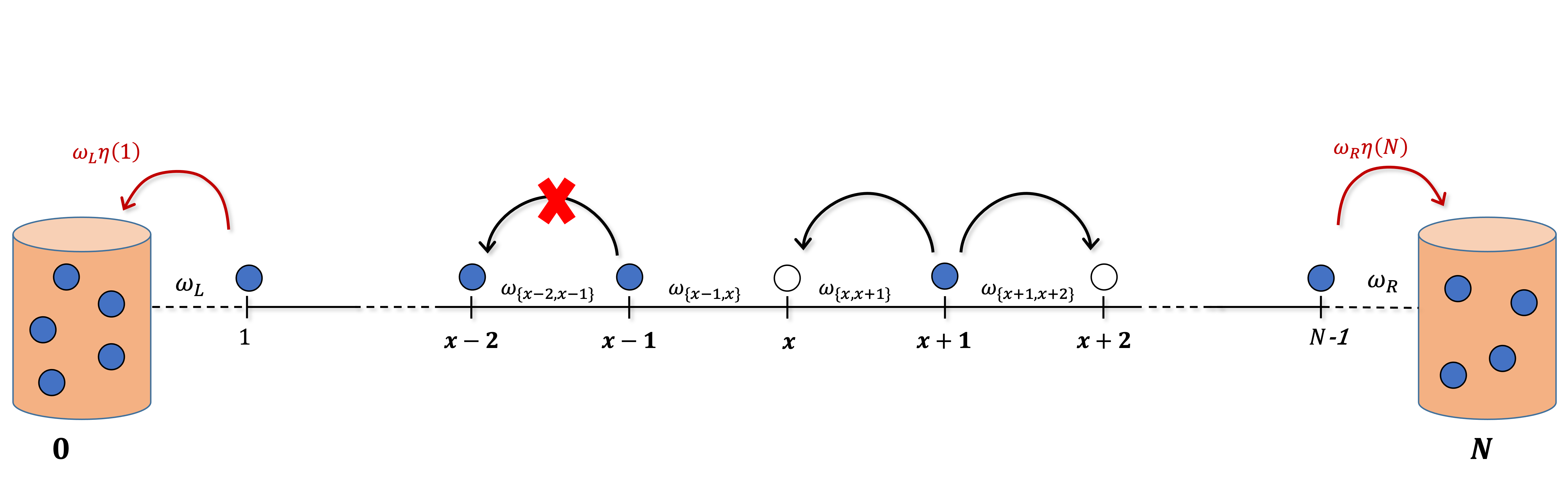
Figure 2. Schematic description of the dual dynamics.

Recall that a configuration $\xi\in\mathcal{\hat{X}}$ will be often identified with the set $I\subset[N]_{0}$ of points $x$ such that $\xi(x)>0$, i.e. $\xi(x)=\boldsymbol{1}_{\{x\in I\}}$, and that we denote by $\hat{\mathbb{P}}_{\xi}$ (or by $\hat{\mathbb{P}}_{I}$) and by $\hat{\mathbb{E}}_{\xi}$ or (by $\hat{\mathbb{E}}_{I}$) the law and the corresponding expectation of the process $(\xi_{t})_{t\geq 0}$ starting from the configuration $\xi$.

For $\eta\in\mathcal{X}$ and $\xi\in\hat{\mathcal{X}}$ we define

$$D(\eta,\xi)=\rho_{L}^{\xi(0)}\left(\prod_{x\in[N-1]:\ \xi(x)=1}\eta(x)\right)\rho_{R}^{\xi(N)}.$$

We recall below the duality relation between the boundary driven SEP and the process $(\xi_{t})_{t\geq 0}$.

Proposition 2.1 (See [6] and [13]).

The boundary driven SEP $(\eta_{t})_{t\geq 0}$ with generator given in (1.1) and the process $(\xi_{t})_{t\geq 0}$ with generatore given in (2.1) satisfy the following relation: for all $\eta\in\mathcal{X}$, $\xi\in\hat{\mathcal{X}}$ and $t\geq 0$

$${\mathbb{E}}_{\eta}[D(\eta_{t},\xi)]=\hat{\mathbb{E}}_{\xi}[D(\eta,\xi_{t})].$$ (2.2)

2.2. The labelled stirring dual process

In order to prove Theorem 1.1 we consider the labelled stirring construction (see, e.g., [9] or [25]) of the dual process on $\hat{G}$. More precisely, define on the same probability space independent random variables $(\Gamma_{x,y})_{\{x,y\}\in E}$, $\Gamma_{0}$, $\Gamma_{N}$ where $\Gamma_{x,y}$ is a Poisson point process with rate $\omega_{x,y}$ providing the swapping times across the edge $\{x,y\}$ and $\Gamma_{0}$ and $\Gamma_{N}$ are Poisson processes with rate $\omega_{L}$ and $\omega_{R}$ respectively, giving the absorbing times from sites $1$ and $N-1$ respectively. The labelled dual particles system $(X^{x_{1}}_{t},\ldots,X^{x_{n}}_{t})_{t\geq 0}$ starting from $x_{1}<\ldots<x_{n}$ is obtained by following deterministically the arrows obtained as a realization of the Poisson processes just introduced. Namely $(X^{x_{1}}_{t},\ldots,X^{x_{n}}_{t})_{t\geq 0}$ is constant until a Poisson mark is encountered. If $t\in\Gamma_{x,y}$ and if at $t^{-}$ there is a particle at $x$ or at $y$ or at both sites, then these particles swap their positions (i.e. if a particle is at $x$ at $t^{-}$ then it moves to $y$ at time $t$ and viceversa), keeping track of their label given by the initial position. If $t\in\Gamma_{0}$ (or $t\in\Gamma_{N}$) and at $t^{-}$ a particle is present at $1$ (or at $N-1$) then that particles is absorbed at $0$ (or at $N$).

For each $n\in[N-1]$ and $x_{1}<\ldots<x_{n}$, we denote by ${\mathbb{P}}^{stir}_{\xi}$ (respectively ${\mathbb{E}}^{stir}_{\xi}$) the probability (respectively the expectation) induced by the random arrows on the space of trajectories of the labelled stirring process started from $\xi=\{x_{1},\ldots,x_{n}\}$.

Notice that by the construction it follows that for al $\Gamma\subset[N]$ and $f:[N]_{0}^{\Gamma}\to{\mathbb{R}}$

$${\mathbb{E}}^{stirr}_{[N]}[f((X^{x}_{t})_{x\in\Gamma})]={\mathbb{E}}^{stirr}_{\Gamma}[f((X^{x}_{t})_{x\in\Gamma})].$$ (2.3)

Moreover, if $f:[N]_{0}^{\Gamma}\to{\mathbb{R}}$ is symmetric (where symmetric means invariant by permutations of its entries), then

$${\mathbb{E}}^{stirr}_{\Gamma}[f((X^{x}_{t})_{x\in\Gamma})]=\hat{\mathbb{E}}_{\Gamma}[f(\xi_{t})].$$ (2.4)

2.3. Probabilistic interpretation of the non-equilibrium steady state and proof of Theorem 1.1

We introduce random variables $(U_{x})_{x\in[N-1]}$ on the same probability space of the stirring construction, with $U_{x}\in\{\rho_{L},\rho_{R}\}$, which are not independent and such that their joint law is given by

$${\mathbb{P}}_{[N-1]}^{stirr}((U_{x})_{x\in[N-1]}=\bar{\rho}_{I})={\mathbb{E}}^{stirr}_{[N-1]}\left[\prod_{x\in I}\boldsymbol{1}_{\{X^{x}_{\infty}=N\}}\prod_{x\in[N-1]\setminus I}\boldsymbol{1}_{\{X^{x}_{\infty}=0\}}\right]$$

where, given $I\subset[N-1]$, $\bar{\rho}_{I}$ is the vector $(\bar{\rho}_{I}(x))_{x\in I}$ with $\bar{\rho}_{I}(x)=\rho_{R}$ if $x\in I$ and $\bar{\rho}_{I}(x)=\rho_{L}$ otherwise.

We start by showing the following result, which clarifies the probabilistic interpretation of the non-equilibrium steady state.

Theorem 2.2.

The stationary distribution of the boundary driven SEP on $G$ with reservoirs parameters $\rho_{L},\rho_{R},\omega_{L},\omega_{R}>0$ is

$$\mu_{\rm{stat}}={\mathbb{E}}^{stirr}_{[N-1]}\left[\otimes_{x\in[N-1]}\rm{Ber}(U_{x})\right].$$ (2.5)

Proof.

The stationary measure $\mu_{\rm{stat}}$ is completely characterized by the moments

$${\mathbb{E}}_{\mu_{\rm{stat}}}\left[\prod_{i=1}^{n}\eta(x_{i})\right],\ \forall n\in[N-1]\ \text{and }\ 1\leq x_{1}<\ldots<x_{n}\leq N-1.$$

By duality, we have

$${\mathbb{E}}_{\mu_{\rm{stat}}}\left[\prod_{i=1}^{n}\eta(x_{i})\right]=\lim_{t\to\infty}{\mathbb{E}}_{\eta}\left[\prod_{i=1}^{n}\eta_{t}(x_{i})\right]$$

$$=\lim_{t\to\infty}\hat{\mathbb{E}}_{\{x_{1},\ldots,x_{n}\}}[D(\eta,\xi_{t})]=\hat{\mathbb{E}}_{\{x_{1},\ldots,x_{n}\}}\left[\rho_{L}^{\xi_{\infty}(0)}\rho_{R}^{\xi_{\infty}(N)}\right]$$

$$=\sum_{\ell=0}^{n}\rho_{R}^{\ell}\rho_{L}^{n-\ell}\hat{\mathbb{P}}_{\{x_{1},\ldots,x_{n}\}}[\xi_{\infty}(N)=\ell].$$ (2.6)

Thus we only need to show that for all $n\in[N-1]$ and $1\leq x_{1}<\ldots<x_{n}\leq N-1$

$$\int\prod_{i=1}^{n}\eta(x_{i})\text{d}{\mathbb{E}}^{stirr}_{[N-1]}\left[\otimes_{x\in[N-1]}\rm{Ber}(U_{x})\right]=\sum_{\ell=0}^{n}\rho_{R}^{\ell}\rho_{L}^{n-\ell}\hat{\mathbb{P}}_{\{x_{1},\ldots,x_{n}\}}[\xi_{\infty}(N)=\ell].$$ (2.7)

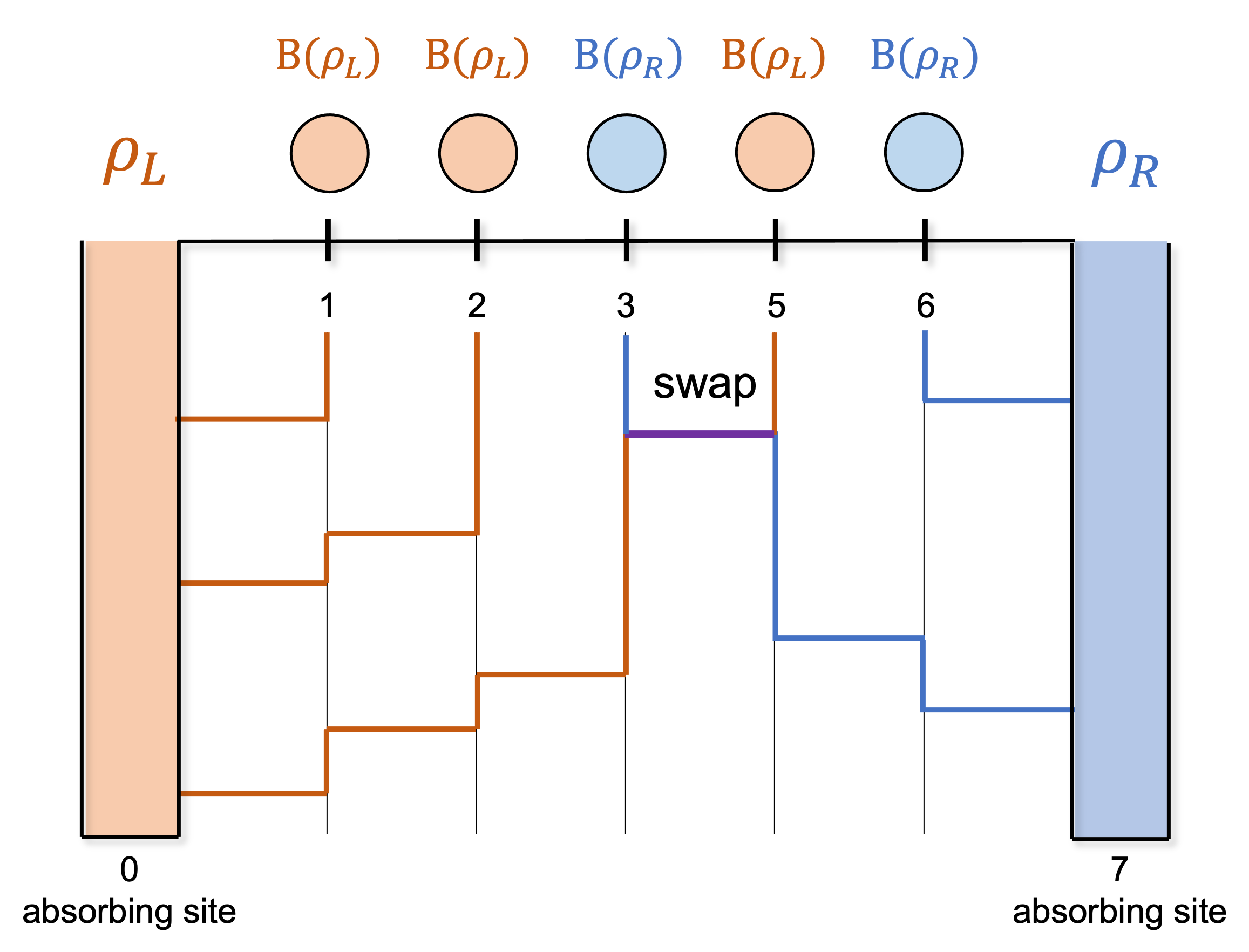
Figure 3. Schematic description of the proof via the stirring construction of the dual process.

We then have, using (2.3),

$$\int\prod_{i=1}^{n}\eta(x_{i})\text{d}{\mathbb{E}}^{stirr}_{[N-1]}\left[\otimes_{x\in[N-1]}\rm{Ber}(U_{x})\right]={\mathbb{E}}^{stirr}_{\{x_{1},\ldots,x_{n}\}}\left[\prod_{i=1}^{n}U_{x_{i}}\right]$$

$$=\sum_{I\subset\{x_{1},\ldots,x_{n}\}}\rho_{R}^{|I|}\rho_{L}^{n-|I|}{\mathbb{E}}^{stirr}_{\{x_{1},\ldots,x_{n}\}}\ \left[\prod_{x\in I}\boldsymbol{1}_{\{X^{x}_{\infty}=N\}}\prod_{x\in\{x_{1},\ldots,x_{n}\}\setminus I}\boldsymbol{1}_{\{X^{x}_{\infty}=0\}}\right]$$

$$=\sum_{\ell=0}^{n}\rho_{R}^{\ell}\rho_{L}^{n-\ell}{\mathbb{E}}^{stirr}_{\{x_{1},\ldots,x_{n}\}}\ \left[\sum_{I\subset\{x_{1},\ldots,x_{n}\}\ :\ |I|=\ell}\left(\prod_{x\in I}\boldsymbol{1}_{\{X^{x}_{\infty}=N\}}\prod_{x\in\{x_{1},\ldots,x_{n}\}\setminus I}\boldsymbol{1}_{\{X^{x}_{\infty}=0\}}\right)\right].$$

Noticing that

$$\sum_{I\subset\{x_{1},\ldots,x_{n}\}\ :\ |I|=\ell}\left(\prod_{x\in I}\boldsymbol{1}_{\{X^{x}_{\infty}=N\}}\prod_{x\in\{x_{1},\ldots,x_{n}\}\setminus I}\boldsymbol{1}_{\{X^{x}_{\infty}=0\}}\right)=\boldsymbol{1}_{\{\sum_{\ell=1}^{n}{\boldsymbol{1}}_{\{X^{x_{\ell}}_{\infty}=N\}}=\ell\}}$$

is a symmetric function and using (2.4), we have that

$${\mathbb{E}}^{stirr}_{\{x_{1},\ldots,x_{n}\}}\left[\sum_{I\subset\{x_{1},\ldots,x_{n}\}\ :\ |I|=\ell}\left(\prod_{x\in I}\boldsymbol{1}_{\{X^{x}_{\infty}=N\}}\prod_{x\in\{x_{1},\ldots,x_{n}\}\setminus I}\boldsymbol{1}_{\{X^{x}_{\infty}=0\}}\right)\right]\\ =\hat{\mathbb{P}}_{\{x_{1},\ldots,x_{n}\}\ }\left(\xi_{\infty}(N)=\ell\right)$$ (2.8)

from which (2.7) follows and in particular (2.5) also follows. ∎

We can finally obtain Theorem 1.1.

Proof of Theorem 1.1.

For any $I\subset[N-1]$

$${\mathbb{P}}^{stirr}_{[N-1]}\left(\cup_{x\in I}\{U_{x}=\rho_{R}\}\cup_{y\in[N-1]\setminus I}\{U_{y}=\rho_{L}\}\right)$$

$$={\mathbb{E}}^{stirr}_{[N-1]}\left[\prod_{x\in I}\boldsymbol{1}_{\{X^{x}_{\infty}=N\}}\prod_{x\in\{x_{1},\ldots,x_{n}\}\setminus I}\boldsymbol{1}_{\{X^{x}_{\infty}=0\}}\right]$$

$$={\mathbb{E}}^{stirr}_{[N-1]}\left[\prod_{x\in I}\boldsymbol{1}_{\{X^{x}_{\infty}=N\}}\prod_{x\in[N-1]\setminus I}\left(1-\boldsymbol{1}_{\{X^{x}_{\infty}=N\}}\right)\right]$$

$$=\sum_{J\subset[N-1]\setminus I}(-1)^{|J|}{\mathbb{E}}^{stirr}_{I\cup J}\left[\prod_{x\in I\cup J}\boldsymbol{1}_{\{X^{x}_{\infty}=N\}}\right]$$

where we used (2.3) in the last equality. Noticing that $\prod_{x\in I\cup J}\boldsymbol{1}_{\{X^{x}_{\infty}=N\}}$ is a symmetric function, using 2.4, we conclude that

$${\mathbb{P}}^{stirr}_{[N-1]}\left(\cup_{x\in I}\{U_{x}=\rho_{R}\}\cup_{y\in[N-1]\setminus I}\{U_{y}=\rho_{L}\}\right)\\ =\sum_{J\subset[N-1]\setminus I}(-1)^{|J|}\hat{\mathbb{P}}_{I\cup J}\left(\xi_{\infty}(N)=|I\cup J|\right)$$ (2.9)

from which we obtain

$${\mathbb{E}}^{stirr}\left[\otimes_{x\in[N-1]}\rm{Ber}(U_{x})\right]=\sum_{J\subset\mathcal{P}([N-1]):\ I\subset J}F(I)\bigg{(}\otimes_{x\in I}\rm{Ber}(\rho_{R})\otimes_{x\in[N-1]\setminus I}\rm{Ber}(\rho_{L})\bigg{)},$$

with $F(I)$ given in (1.3) and thus the thesis of Theorem 1.1.

∎

2.4. Proofs of Proposition 1.5 and Proposition 1.6

We conclude the section by proving Proposition 1.5 and Proposition 1.6 which are also achieved by duality.

Proof of Proposition 1.5.

Arguing as in the Proof of Theorem 1.1, we obtain

$$\hat{\mathbb{P}}_{\{x_{1},\ldots,x_{n}\}}(\xi_{\infty}(N)=\ell)$$

$$=\sum_{I\subset\{x_{1},\ldots,x_{n}\}\ :\ |I|=\ell}\quad{\mathbb{E}}^{stirr}_{\{x_{1},\ldots,x_{n}\}}\ \left[\prod_{x\in I}\boldsymbol{1}_{\{X^{x}_{\infty}=N\}}\prod_{x\in\{x_{1},\ldots,x_{n}\}\setminus I}\boldsymbol{1}_{\{X^{x}_{\infty}=0\}}\right]$$

$$=\sum_{I\subset\{x_{1},\ldots,x_{n}\}\ :\ |I|=\ell}\quad{\mathbb{E}}^{stirr}_{\{x_{1},\ldots,x_{n}\}}\ \left[\prod_{x\in I}\boldsymbol{1}_{\{X^{x}_{\infty}=N\}}\prod_{x\in\{x_{1},\ldots,x_{n}\}\setminus I}(1-\boldsymbol{1}_{\{X^{x}_{\infty}=N\}})\right]$$

$$=\sum_{I\subset\{x_{1},\ldots,x_{n}\}\ :\ |I|=\ell}\ \sum_{J\subset\{x_{1},\ldots,x_{n}\}\setminus I}(-1)^{|J|}\hat{\mathbb{P}}_{I\cup J}(\xi_{\infty}(N)=|I\cup J|).$$

Exchanging the order of the above summations we get

$$\hat{\mathbb{P}}_{\{x_{1},\ldots,x_{n}\}}(\xi_{\infty}(N)=\ell)$$

$$=\sum_{K\subset\{x_{1},\ldots,x_{n}\}\ :\ |K|\geq\ell}\hat{\mathbb{P}}_{K}(\xi_{\infty}(N)=|K|)\left(\sum_{I\subset K\ :\ |I|=\ell}(-1)^{|K|-|I|}\right)$$

$$=\sum_{K\subset\{x_{1},\ldots,x_{n}\}\ :\ |K|\geq\ell}(-1)^{|K|-\ell}{{|K|}\choose{\ell}}\hat{\mathbb{P}}_{K}(\xi_{\infty}(N)=|K|)$$

concluding the proof. ∎

Proof of Proposition 1.6.

For what concerns the centered $n$ point correlations, equations (1.6) and (1.7) follows by the combination of Theorem 1.4 above (which is proved in Section 3 and Section 4 below with two different approaches) with [13, Theorem 5.1].

For what concerns the non-centered $n$ point correlations, recall from (2.3) that

$${\mathbb{E}}_{\mu_{\rm{stat}}}\left[\prod_{i=1}^{n}\eta(x_{i})\right]=\sum_{\ell=0}^{n}\rho_{R}^{\ell}\rho_{L}^{n-\ell}\hat{\mathbb{P}}_{\{x_{1},\ldots,x_{n}\}}[\xi_{\infty}(N)=\ell].$$

Employing Proposition 1.5 we obtain

$${\mathbb{E}}_{\mu_{\rm{stat}}}\left[\prod_{i=1}^{n}\eta(x_{i})\right]=\sum_{\ell=0}^{n}\rho_{R}^{\ell}\rho_{L}^{n-\ell}\sum_{k=\ell}^{n}(-1)^{k-\ell}{{k}\choose{\ell}}\sum_{1\leq i_{1}<\ldots<i_{k}\leq n}\hat{\mathbb{P}}_{\{x_{i_{1}},\ldots,x_{i_{k}}\}}(\xi_{\infty}(N)=k)$$

and changing the order of summations we have

$${\mathbb{E}}_{\mu_{\rm{stat}}}\left[\prod_{i=1}^{n}\eta(x_{i})\right]=\sum_{k=0}^{n}\ \sum_{1\leq i_{1}<\ldots<i_{k}\leq n}\hat{\mathbb{P}}_{\{x_{i_{1}},\ldots,x_{i_{k}}\}}(\xi_{\infty}(N)=k)\sum_{\ell=0}^{k}(-1)^{k-\ell}{{k}\choose{\ell}}\rho_{R}^{\ell}\rho_{L}^{n-\ell}$$

$$=\sum_{k=0}^{n}\ \sum_{1\leq i_{1}<\ldots<i_{k}\leq n}\hat{\mathbb{P}}_{\{x_{i_{1}},\ldots,x_{i_{k}}\}}(\xi_{\infty}(N)=k)\rho_{L}^{n-k}\sum_{\ell=0}^{k}{{k}\choose{\ell}}\rho_{R}^{\ell}(-\rho_{L})^{k-\ell}$$

$$=\sum_{k=0}^{n}\rho_{L}^{n-k}(\rho_{R}-\rho_{L})^{k}\sum_{1\leq i_{1}<\ldots<i_{k}\leq n}\hat{\mathbb{P}}_{\{x_{i_{1}},\ldots,x_{i_{k}}\}}(\xi_{\infty}(N)=k)$$

and employing Theorem 1.4 above we conclude the proof.

∎

3. 2-point correlations and the absorption probabilities via induction

In this section, our objective is to calculate the two-point stationary correlations for the boundary driven SSEP on a segment where all the conductances are set to one, except for the conductances that connect site $1$ with the left reservoir and site $N-1$ with the right reservoir. Thus we consider the $\alpha$, $\beta$, $\gamma$, $\delta$ model and we allow the possibility to rescale the intensity of the conductances connected to reservoirs as done in hydrodynamic limits (see [19]).

Because by duality, this amount to compute the absorption probabilities of two dual interacting particles, we start by computing such quantities in Subsection 3.1 below. Based on the resulting expression, we then make an educated guess for the absorption probability of an arbitrary number of particles, which we subsequently prove to be true by induction in Subsection 3.2 below.

Additionally, in Section 4 below, we present an alternative approach to compute the absorption probabilities. This method relies on a probabilistic coupling technique that eliminates the need to make assumptions regarding the specific form of these probabilities.

3.1. 2-point correlations via three martingales

Consider the open SSEP on the homogeneous segment $([N-1],E,(\omega_{x,y})_{\{x,y\}\in E})$, with $\{x,y\}\in E$ if and only if $|x-y|=1$, $\omega_{x,x+1}=1$ for each $x\in\{1,\ldots,N-2\}\in E$, and set $\omega_{L},\omega_{R}>0$.

We prove the following expression for the two point centered correlation previously derived in [31] and [12] via other methods.

Proposition 3.1.

For $x<y$

$$\rm{Cor}(x,y):= \hat{\mathbb{E}}_{\mu_{\rm{stat}}}[\eta(x)\eta(y)]-\hat{\mathbb{E}}_{\mu_{\rm{stat}}}[\eta(x)]\hat{\mathbb{E}}_{\mu_{\rm{stat}}}[\eta(y)]$$

$$=-(\rho_{R}-\rho_{L})^{2}\frac{\left(\frac{1}{\omega_{L}}+x-1\right)\left(\frac{1}{\omega_{R}}+N-1-y\right)}{\left(\frac{1}{\omega_{L}}+\frac{1}{\omega_{R}}+N-2\right)^{2}\left(\frac{1}{\omega_{L}}+\frac{1}{\omega_{R}}+N-3\right)}.$$

We achieve the above result by computing the absorption probabilities of two dual particles evolving on the extended segment $[N-1]\cup\{0,N\}$, where $\{0,N\}$ are the two absorbing sites. In particular, in order to compute asymptotic absorption probabilities, it is enough to consider the skeleton chain of the dual process $(\xi_{t})_{t\geq 0}$ starting from $\xi_{0}=\{x,y\}$. Denote by $(X^{x}_{n},X^{y}_{n})$ the position of two dual particles starting from $x<y$, where swapping is not allowed, after $n$ steps (i.e. $n$ is the number of jumps). Notice that $X^{x}_{n}=X^{y}_{n}$ if and only if $X^{x}_{n}=X^{y}_{n}\in\{0,N\}$, i.e. both particles are eventually absorbed in the same site.

Recall that in a segment weighted by symmetric conductances $\omega_{x,x+1}$, harmonic functions at $z$ are given by

$$\sum_{i=0}^{z-1}\frac{1}{\omega_{i,i+1}}+\text{constant}.$$

Thus, in our setting we set

$$\begin{cases}h(0):=0\\ h(x):=\frac{1}{\omega_{L}}+x-1,\quad x\in\{1,\ldots,N-1\}\\ h(N):=\frac{1}{\omega_{L}}+\frac{1}{\omega_{R}}+N-2\end{cases}$$ (3.1)

and the absorption probability on the point $N$ of a particle starting from $x\in[N]_{0}$ is then given by

$$\hat{\mathbb{P}}_{\{x\}}[\xi_{\infty}(N)=1]=\frac{h(x)}{h(N)}.$$

In order to compute the absorption probabilities we take advantage of three martingales with respect to the natural filtration generated by $\{X^{x}_{n},X^{y}_{n}\}_{n\in{\mathbb{N}}}$ which are given in Lemma below.

Lemma 3.2.

Let $x<y$ and define the following process

$$D_{0}=0$$

$$D_{n}:=\sum_{k=0}^{n-1}{\boldsymbol{1}}_{\{X^{y}_{k}-X^{x}_{k}=1\}}{\boldsymbol{1}}_{\{X^{y}_{k},X^{x}_{k}\notin\{0,N\}\}}\\ \times\left({\boldsymbol{1}}_{\{X^{y}_{k},X^{x}_{k}\notin\{1,N-1\}\}}+\frac{2}{\omega_{L}+1}{\boldsymbol{1}}_{\{X^{x}_{k}=1\}}+\frac{2}{\omega_{R}+1}{\boldsymbol{1}}_{\{X^{y}_{k}=N-1\}}\right).$$ (3.2)

Then the processes

$$(h(X^{x}_{n})+h(X^{y}_{n}))_{n\geq 0},$$ (3.3)

$$(h(X^{y}_{n})-h(X^{x}_{n})-D_{n})_{n\geq 0}$$ (3.4)

and

$$(h(X^{x}_{n})h(X^{y}_{n})+\frac{1}{2}D_{n})_{n\geq 0}$$ (3.5)

are martingales with respect to the filtration $\mathcal{F}_{n}:=\sigma\{X^{x}_{k},X^{y}_{k},k\in\{0,\ldots,n\}\}$.

Proof.

We provide only the proof of the fact that $(h(X^{x}_{n})h(X^{y}_{n})+\frac{1}{2}D_{n})_{n\geq 0}$ is a martingale since for the other two processes the conclusion follows by similar arguments.

Denote by $\hat{\mathbb{E}}_{(x,y)}$ the expectation of the skeleton chain $\{X^{x}_{n},X^{y}_{n}\}_{n\in{\mathbb{N}}}$. We need to show that

$$\hat{\mathbb{E}}_{(x,y)}\left[h(X^{x}_{n})h(X^{y}_{n})+\frac{1}{2}D_{n}|\mathcal{F}_{n-1}\right]=h(X^{x}_{n-1})h(X^{y}_{n-1})+\frac{1}{2}D_{n-1}.$$ (3.6)

Let us now write

$$1 =(1-{\boldsymbol{1}}_{\{X^{y}_{n-1},X^{x}_{n-1}\notin\{0,N\}\}})$$

$$+{\boldsymbol{1}}_{\{X^{y}_{n-1},X^{x}_{n-1}\notin\{0,N\}\}}\left({\boldsymbol{1}}_{\{X^{y}_{n-1}-X^{x}_{n-1}\neq 1\}}\right.$$

$$\left.+{\boldsymbol{1}}_{\{X^{y}_{n-1}-X^{x}_{n-1}=1\}}\left({\boldsymbol{1}}_{\{X^{y}_{n-1},X^{x}_{n-1}\notin\{1,N-1\}\}}\right.\right.$$

$$\left.\left.+\frac{1}{\omega_{L}+1}{\boldsymbol{1}}_{\{X^{x}_{n-1}=1\}}+\frac{1}{\omega_{R}+1}{\boldsymbol{1}}_{\{X^{y}_{n-1}=N-1\}}\right)\right).$$ (3.7)

First notice that if at time $n-1$ both particles are absorbed, then no extra jumps occur. If only one particle is absorbed at time $n-1$ then $D_{n-1}=D_{n}$, the particle not absorbed is an independent random walk and because $h$ is harmonic, we conclude

$$\hat{\mathbb{E}}_{(x,y)}\left[(1-{\boldsymbol{1}}_{\{X^{y}_{n-1},X^{x}_{n-1}\notin\{0,N\}\}})(h(X^{x}_{n})h(X^{y}_{n})+\frac{1}{2}D_{n})|\mathcal{F}_{n-1}\right]\\ =(1-{\boldsymbol{1}}_{\{X^{y}_{n-1},X^{x}_{n-1}\notin\{0,N\}\}})(h(X^{x}_{n-1})h(X^{y}_{n-1})+\frac{1}{2}D_{n-1}).$$ (3.8)

Consider now

$$\hat{\mathbb{E}}_{(x,y)}\left[{\boldsymbol{1}}_{\{X^{y}_{n-1},X^{x}_{n-1}\notin\{0,N\}\}}{\boldsymbol{1}}_{\{X^{y}_{n-1}-X^{x}_{n-1}\neq 1\}}(h(X^{x}_{n})h(X^{y}_{n})+\frac{1}{2}D_{n})|\mathcal{F}_{n-1}\right].$$

On the event ${\boldsymbol{1}}_{\{X^{y}_{n-1}-X^{x}_{n-1}\neq 1\}}$ we have $D_{n}=D_{n-1}$ and since particles are not nearest neighbor, they behave as independent random walks an thus

$$\hat{\mathbb{E}}_{(x,y)}\left[{\boldsymbol{1}}_{\{X^{y}_{n-1},X^{x}_{n-1}\notin\{0,N\}\}}{\boldsymbol{1}}_{\{X^{y}_{n-1}-X^{x}_{n-1}=1\}}(h(X^{x}_{n})h(X^{y}_{n})+\frac{1}{2}D_{n})|\mathcal{F}_{n-1}\right]\\ ={\boldsymbol{1}}_{\{X^{y}_{n-1},X^{x}_{n-1}\notin\{0,N\}\}}{\boldsymbol{1}}_{\{X^{y}_{n-1}-X^{x}_{n-1}\neq 1\}}(h(X^{x}_{n-1})h(X^{y}_{n-1})+\frac{1}{2}D_{n-1}).$$ (3.9)

Denote by

$$A:={\boldsymbol{1}}_{\{X^{y}_{n-1},X^{x}_{n-1}\notin\{0,N\}\}}{\boldsymbol{1}}_{\{X^{y}_{n-1}-X^{x}_{n-1}=1\}}{\boldsymbol{1}}_{\{X^{y}_{n-1},X^{x}_{n-1}\notin\{1,N-1\}\}}$$

and notice that in this case

$$\hat{\mathbb{E}}_{(x,y)}\left[AD_{n}|\mathcal{F}_{n-1}\right]=A(D_{n-1}+1).$$

Moreover

$$\hat{\mathbb{E}}_{(x,y)}\left[Ah(X^{x}_{n})h(X^{y}_{n})|\mathcal{F}_{n-1}\right]=A\hat{\mathbb{E}}_{(X^{x}_{n-1},X^{y}_{n-1})}\left[h(X^{x}_{n})h(X^{y}_{n})\right]$$

$$=A\left(\frac{1}{2}h(X^{x}_{n-1}-1)h(X^{y}_{n-1})+\frac{1}{2}h(X^{x}_{n-1})h(X^{y}_{n-1}+1)\right)$$

$$=Ah(X^{x}_{n-1})h(X^{y}_{n-1})-\frac{1}{2}A(h(X^{y}_{n-1})-h(X^{x}_{n-1}))$$

$$=Ah(X^{x}_{n-1})h(X^{y}_{n-1})-\frac{1}{2}A$$

from which we obtain

$$\hat{\mathbb{E}}_{(x,y)}\left[A(h(X^{x}_{n})h(X^{y}_{n})+\frac{1}{2}D_{n})|\mathcal{F}_{n-1}\right]=A(h(X^{x}_{n-1})h(X^{y}_{n-1})+\frac{1}{2}D_{n-1}).$$

Denote by

$$B:={\boldsymbol{1}}_{\{X^{y}_{n-1},X^{x}_{n-1}\notin\{0,N\}\}}{\boldsymbol{1}}_{\{X^{y}_{n-1}-X^{x}_{n-1}=1\}}{\boldsymbol{1}}_{\{X^{x}_{n-1}=1\}}$$

and notice that in this case

$$\hat{\mathbb{E}}_{(x,y)}\left[BD_{n}|\mathcal{F}_{n-1}\right]=B(D_{n-1}+\frac{2}{\omega_{L}+1}).$$

Moreover

$$\hat{\mathbb{E}}_{(x,y)}\left[Bh(X^{x}_{n})h(X^{y}_{n})|\mathcal{F}_{n-1}\right]=B\hat{\mathbb{E}}_{(X^{x}_{n-1},X^{y}_{n-1})}\left[h(X^{x}_{n})h(X^{y}_{n})\right]$$

$$=B\left(\frac{\omega_{L}}{1+\omega_{L}}h(X^{x}_{n-1}-1)h(X^{y}_{n-1})+\frac{1}{1+\omega_{L}}h(X^{x}_{n-1})h(X^{y}_{n-1}+1)\right)$$

$$=0+B\frac{1}{1+\omega_{L}}\left(h(X^{x}_{n-1})h(X^{y}_{n-1})+h(X^{x}_{n-1})\right)$$

$$=Bh(X^{x}_{n-1})h(X^{y}_{n-1})-\frac{B}{1+\omega_{L}}(h(X^{y}_{n-1})-h(X^{x}_{n-1}))$$

$$=Bh(X^{x}_{n-1})h(X^{y}_{n-1})-\frac{B}{1+\omega_{L}}$$

from which we obtain

$$\hat{\mathbb{E}}_{(x,y)}\left[B(h(X^{x}_{n})h(X^{y}_{n})+\frac{1}{2}D_{n})|\mathcal{F}_{n-1}\right]=B(h(X^{x}_{n-1})h(X^{y}_{n-1})+\frac{1}{2}D_{n-1}).$$

Denote by

$$C:={\boldsymbol{1}}_{\{X^{y}_{n-1},X^{x}_{n-1}\notin\{0,N\}\}}{\boldsymbol{1}}_{\{X^{y}_{n-1}-X^{x}_{n-1}=1\}}{\boldsymbol{1}}_{\{X^{y}_{n-1}=N-1\}}$$

and notice that in this case

$$\hat{\mathbb{E}}_{(x,y)}\left[CD_{n}|\mathcal{F}_{n-1}\right]=C(D_{n-1}+\frac{2}{\omega_{R}+1}).$$

Moreover

$$\hat{\mathbb{E}}_{(x,y)}\left[Ch(X^{x}_{n})h(X^{y}_{n})|\mathcal{F}_{n-1}\right]=C\hat{\mathbb{E}}_{(X^{x}_{n-1},X^{y}_{n-1})}\left[h(X^{x}_{n})h(X^{y}_{n})\right]$$

$$=C\left(\frac{1}{1+\omega_{R}}h(X^{x}_{n-1}-1)h(X^{y}_{n-1})+\frac{\omega_{R}}{1+\omega_{R}}h(X^{x}_{n-1})h(X^{y}_{n-1}+1)\right)$$

$$=\frac{C}{1+\omega_{R}}\left[\left(h(X^{x}_{n-1})h(X^{y}_{n-1})-h(X^{y}_{n-1})\right)+\omega_{R}\left(h(X^{x}_{n-1})h(X^{y}_{n-1})+\frac{1}{\omega_{R}}h(X^{x}_{n-1})\right)\right]$$

$$=Ch(X^{x}_{n-1})h(X^{y}_{n-1})-\frac{C}{1+\omega_{R}}(h(X^{y}_{n-1})-h(X^{x}_{n-1}))$$

$$=Ch(X^{x}_{n-1})h(X^{y}_{n-1})-\frac{C}{1+\omega_{R}}$$

from which we obtain

$$\hat{\mathbb{E}}_{(x,y)}\left[C(h(X^{x}_{n})h(X^{y}_{n})+\frac{1}{2}D_{n})|\mathcal{F}_{n-1}\right]=C(h(X^{x}_{n-1})h(X^{y}_{n-1})+\frac{1}{2}D_{n-1}).$$

Putting everything together and recalling (3.1) we obtain (3.6), and thus that the process $(h(X^{x}_{n})h(X^{y}_{n})+\frac{1}{2}D_{n})_{n\geq 0}$ is a martingale.

∎

We can thus prove Proposition 3.1.

Proof of Proposition 3.1.

By employing the martingales of Lemma 3.2 above and sending $n$ to infinity we obtain (by Doob’s optional sampling theorem), for $x<y$,

$$\begin{cases}h(x)+h(y)=2h(N)\hat{\mathbb{P}}_{\{x,y\}}[\xi_{\infty}(N)=2]+h(N)\hat{\mathbb{P}}_{\{x,y\}}[\xi_{\infty}(N)=1]\\ h(y)-h(x)=h(N)\hat{\mathbb{P}}_{\{x,y\}}[\xi_{\infty}(N)=1]-\hat{\mathbb{E}}_{(x,y)}[D_{\infty}]\\ h(x)h(y)=h(N)^{2}\hat{\mathbb{P}}_{\{x,y\}}[\xi_{\infty}(N)=1]+\frac{1}{2}\hat{\mathbb{E}}_{(x,y)}[D_{\infty}]\end{cases}$$ (3.10)

and thus

$$\hat{\mathbb{P}}_{\{x,y\}}[\xi_{\infty}(N)=2]=\frac{h(x)(h(y)-1)}{h(N)(h(N)-1)},$$ (3.11)

$$\hat{\mathbb{P}}_{\{x,y\}}[\xi_{\infty}(N)=1]=\frac{h(x)+h(y)}{h(N)}-2\frac{h(x)(h(y)-1)}{h(N)(h(N)-1)}$$ (3.12)

and

$$\hat{\mathbb{P}}_{\{x,y\}}[\xi_{\infty}(N)=0] =1-\hat{\mathbb{P}}_{\{x,y\}}[\xi_{\infty}(N)=2]-\hat{\mathbb{P}}_{\{x,y\}}[\xi_{\infty}(N)=1]$$

$$=1-\frac{h(x)+h(y)}{h(N)}+\frac{h(x)(h(y)-1)}{h(N)(h(N)-1)}.$$ (3.13)

Writing

$$\hat{\mathbb{E}}_{\mu_{\rm{stat}}}[\eta(x)\eta(y)]=\rho_{L}^{2}\hat{\mathbb{P}}_{\{x,y\}}[\xi_{\infty}(N)=0]\\ +\rho_{L}\rho_{R}\hat{\mathbb{P}}_{\{x,y\}}[\xi_{\infty}(N)=1]+\rho_{R}^{2}\hat{\mathbb{P}}_{\{x,y\}}[\xi_{\infty}(N)=2]$$

and

$$\hat{\mathbb{E}}_{\mu_{\rm{stat}}}[\eta(x)]\hat{\mathbb{E}}_{\mu_{\rm{stat}}}[\eta(y)]$$

$$=\rho_{R}^{2}\hat{\mathbb{P}}_{\{x\}}[\xi_{\infty}(N)=1]\hat{\mathbb{P}}_{\{y\}}[\xi_{\infty}(N)=1]$$

$$+\rho_{R}\rho_{L}(\hat{\mathbb{P}}_{\{x\}}[\xi_{\infty}(N)=0]\hat{\mathbb{P}}_{\{y\}}[\xi_{\infty}(N)=1]+\hat{\mathbb{P}}_{\{x\}}[\xi_{\infty}(N)=1]\hat{\mathbb{P}}_{\{x\}}[\xi_{\infty}(N)=0])$$

$$+\rho_{L}^{2}\hat{\mathbb{P}}_{\{x\}}[\xi_{\infty}(N)=0]\hat{\mathbb{P}}_{\{x\}}[\xi_{\infty}(N)=0]$$

and recalling that $\hat{\mathbb{P}}_{\{x\}}[\xi_{\infty}(N)=1]=\frac{h(x)}{h(N)}$, we finally obtain, using (3.11), (3.12) and (3.1), the desired identity. ∎

3.2. Absorption probabilities via induction

In the proof above we showed that for $x<y$,

$$\hat{\mathbb{P}}_{\{x,y\}}[\xi_{\infty}(N)=2] =\frac{h(x)(h(y)-1)}{h(N)(h(N)-1)}$$ (3.14)

$$=\frac{\frac{1}{\omega_{L}}+x-1}{\frac{1}{\omega_{L}}+\frac{1}{\omega_{R}}+(N-1)-1}\frac{\frac{1}{\omega_{L}}+y-2}{\frac{1}{\omega_{L}}+\frac{1}{\omega_{R}}+(N-1)-2}.$$ (3.15)

From the formula above we can make a guess for the absorption probability that starting with $k$ particles all of them are absorbed at $N$ and then prove that our guess is correct by induction.

Lemma 3.3.

Recall the function $h$ given in (3.1). Then, given $1\leq x_{1}<\ldots<x_{k}\leq N-1$,

$$\hat{\mathbb{P}}_{\{x_{1},\ldots,x_{k}\}}[\xi_{\infty}(N)=k]=\prod_{i=1}^{k}\frac{h(x_{i})-(i-1)}{h(N)-(i-1)}.$$ (3.16)

Proof.

First notice that the formula matches the boundary conditions of the absorption probability. Second, assume that the formula holds for $k-1$ and let us show that

$$\hat{\mathcal{L}}\left(\prod_{i=1}^{k}\frac{h(x_{i})-(i-1)}{h(N)-(i-1)}\right)=0.$$

Define

$$g_{k}(x_{1},\ldots,x_{k}):=\prod_{i=1}^{k}\frac{h(x_{i})-(i-1)}{h(N)-(i-1)}.$$

If $x_{k}>x_{k-1}+1$ then we can apply the dual generator in the following way

$$\hat{\mathcal{L}}g_{k}(x_{1},\ldots,x_{k})$$

$$=\left(\hat{\mathcal{L}}g_{k-1}(x_{1},\ldots,x_{k-1})\right)\frac{h(x_{k})-(k-1)}{h(N)-(k-1)}$$

$$+g_{k-1}(x_{1},\ldots,x_{k-1})\hat{\mathcal{L}}\left(\frac{h(x_{k})-(k-1)}{h(N)-(k-1)}\right)=0$$

where the last equality follows by the induction assumption and the fact that $h$ is harmonic for $\hat{\mathcal{L}}$. If $x_{k}=x_{k-1}+1$ and $x_{k+1}\neq N-1$ then we can apply the generator in the following way

$$\hat{\mathcal{L}}\left(\prod_{i=1}^{k}\frac{h(x_{i})-(i-1)}{h(N)-(i-1)}\right)$$

$$=\left(\hat{\mathcal{L}}g_{k-1}(x_{1},\ldots,x_{k-1})\right)\frac{h(x_{k})-(k-1)}{h(N)-(k-1)}$$

$$-g_{k-2}(x_{1},\ldots,x_{k-2})\left(\frac{h(x_{k-1}+1)-(k-2)}{h(N)-(k-2)}-\frac{h(x_{k-1})-(k-2)}{h(N)-(k-2)}\right)\frac{h(x_{k})-(k-1)}{h(N)-(k-1)}$$

$$+g_{k-1}(x_{1},\ldots,x_{k-1})\left(\frac{h(x_{k}+1)-(k-1)}{h(N)-(k-1)}-\frac{h(x_{k})-(k-1)}{h(N)-(k-1)}\right)=0$$

where the first term on the right hand side is zero by induction and the second term, which appears because in the first term of the right hand side we applied the generator as if the $k+1$ particle was not present in the system, cancel the third term. Similarly, if $x_{k}=x_{k-1}+1$ and $x_{k+1}=N-1$ the difference is that the third term on the right hand side of the computation above is multiplied by $\omega_{R}$ which however cancel with $h(x_{k}+1)-h(x_{k})=\frac{1}{\omega_{R}}$ and thus again $\hat{\mathcal{L}}\left(\prod_{i=1}^{k}\frac{h(x_{i})-(i-1)}{h(N)-(i-1)}\right)=0$ concluding the proof. ∎

4. n-point correlations via the Ninja particle method

The matrix ansatz method of [10] allow to derive a recursive relation for the correlations of the boundary driven SSEP (see [11, (A.7)]). As pointed out in [7, Section 7.1], from such relation satisfied by the correlations, an analogous relation for the absorption probabilities in the dual system follows. However, so far a probabilistic approach alternative to the matrix ansatz method has not been proposed.

In this section we provide a probabilistic route to compute the absorption probabilities of the dual process by building a coupling between two dual boundary driven SSEP, one evolving on $[N]_{0}$ and the other one on $[N-1]_{0}$ from which we deduce a recursive relation for the absorption probabilities in the two systems. In the following we consider the homogeneous segment, i.e. $\{x,y\}\in E$ if and only if $|x-y|=1$, $\omega_{x,x+1}=1$ for each $x\in\{1,\ldots,N-2\}\in E$ and we put $\omega_{L}=\omega_{R}=1$ as well. We denote by $(\xi^{[M]}_{t})_{t\geq 0}$ the dual boundary driven SSEP on the homogeneous segment $[M]_{0}$ where $\{0,M\}$ are absorbing sites and by $\hat{\mathbb{P}}^{[M]_{0}}_{\{x_{1},\ldots,x_{k}\}}$ the law of $(\xi^{[M]}_{t})_{t\geq 0}$ starting from $\sum_{i=1}^{k}\delta_{x_{i}}$. Moreover we denote by $\hat{\mathcal{L}}^{[M]_{0}}$ the generator of $(\xi^{[M]}_{t})_{t\geq 0}$.

The main result of the section is the following theorem.

Theorem 4.1.

For all $0\leq x_{1}<\ldots<x_{k+1}\leq N$ the following relation holds

$$\hat{\mathbb{P}}^{[N]_{0}}_{\{x_{1},\ldots,x_{k+1}\}}(\xi^{[N]_{0}}_{\infty}(N)=k+1)=\left(\frac{x_{k+1}-k}{N}\right)\ \hat{\mathbb{P}}^{[N-1]_{0}}_{\{x_{1},\ldots,x_{k}\}}(\xi^{[N-1]_{0}}_{\infty}(N)=k).$$ (4.1)

Recalling that $\hat{\mathbb{P}}^{[N]_{0}}_{\{x\}}(\xi^{[N]_{0}}_{\infty}(N)=1)=\frac{x}{N}$, as a direct consequence of the above theorem, we obtain the explicit absorption probabilities.

Corollary 4.2.

Let $0<x_{1}<\ldots<x_{n}<N$, then

$$\hat{\mathbb{P}}^{[N]_{0}}_{\{x_{1},\ldots,x_{k}\}}(\xi^{[N]_{0}}_{\infty}(N)=k)=\prod_{i=1}^{k}\frac{x_{i}-(i-1)}{N-(i-1)}.$$ (4.2)

In the next section we present the coupling we mentioned above. This technique relies on the introduction of a special particle, denoted by Ninja, which has some special features reminiscent of the behavior of second class particles (see, e.g., [24, pag. 218]) and will be responsible for the coupling of the two processes on different graphs.

4.1. The Ninja-process: a game of labels

Consider the homogeneous segment $[N]_{0}=[N-1]\cup\{0,N\}$ where $\{0,N\}$ are absorbing sites.

We place $k+1$ particles initially at distinct positions $x_{1},\ldots,x_{k+1}\in[N]_{0}$ with

$$1\leq x_{1}<\ldots<x_{k}\leq N-1$$

and

$$x_{k+1}\notin\{x_{1},\ldots,x_{k}\}$$

and we label by $(i)$ the particle starting from $x_{i}$ for all $i\in\{1,\ldots,k\}$ and by Ninja, the particle starting at $x_{k+1}$ (see Figure 4). We do not allow the following two cases:

$$\exists i\in\{1,\ldots,k\}\ s.t.\ x_{i}=N-1\ \text{and }x_{k+1}=N$$

and

$$\exists i\in\{1,\ldots,k\}\ s.t.\ x_{i}=1\ \text{and }x_{k+1}=0.$$

For our purposes we will be interested in the case $x_{k+1}>x_{i}$ for all $i\in\{1,\ldots,k\}$, but the process that we are going to define does not require such condition. We are now going to describe in words the dynamics of the process

$$(X^{(1)}_{t},\ldots,X^{(k)}_{t},\textit{Ninja}_{t})_{t\geq 0}$$

that we call Ninja-process with law denoted by ${\mathbb{P}}^{\textit{Ninja}}_{x_{1},\ldots,x_{k+1}}$.

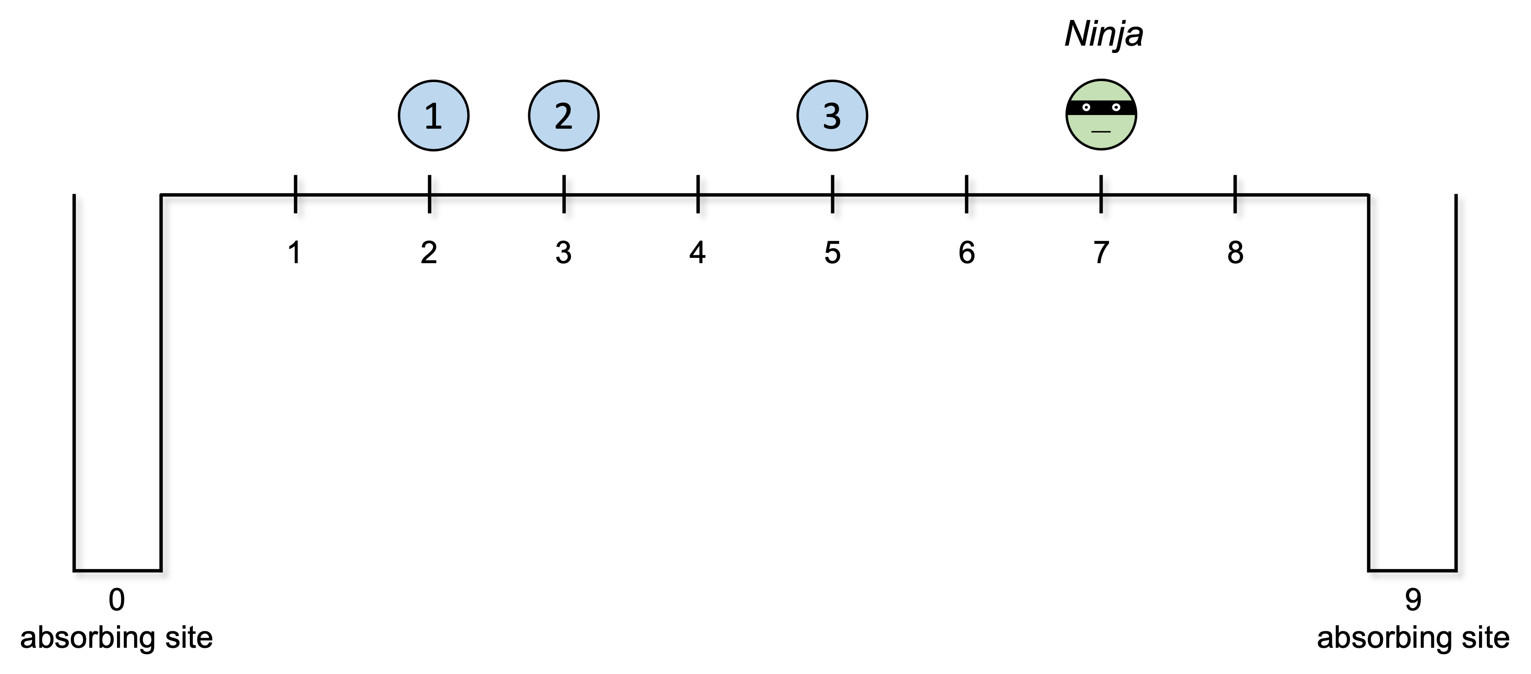
Figure 4.

The particles will move in such a way that the configuration process obtained by the labelled particles evolve exactly as the usual dual of the boundary driven SSEP on $[N]_{0}$ but we play with the labels of the particles and more precisely with the Ninja label in order to perform the coupling. More precisely:

• (The Ninja is alone) When no particle is in a location nearest neighbor to the Ninja and the $\textit{Ninja}\notin\{0,N\}$ each particle, including the Ninja, behaves as simple symmetric random walks jumping at rate one, subject to the exclusion rule and with $\{0,N\}$ acting as absorbing sites. In this case, the Ninja does not have nearest neighbor particles and it jumps at rate one either to its left or to its right.

• (The Ninja interacts) Consider now the case in which the Ninja particle is not at $\{0,N\}$ and the $i$-th particle, with $i\in\{1,\ldots,k\}$, is nearest neighbor of the Ninja and not in $\{0,N\}$. Then all the other particles that are not nearest neighbor of the Ninja behave as simple symmetric random walks jumping at rate one, subject to the exclusion rule and with $\{0,N\}$ acting as absorbing sites. On the other hand the couple $(x_{i},\textit{Ninja})$ jumps at rate one to

  $$(x_{i}+2(\textit{Ninja}-x_{i}),x_{i})$$

  if the site $x_{i}+2(\textit{Ninja}-x_{i})$ is empty and at rate one to

  $$(x_{i}-(\textit{Ninja}-x_{i}),\textit{Ninja})$$

  if $x_{i}-(\textit{Ninja}-x_{i})$ is empty (see Figures 5 and 6). Similarly if there exists another index $j\neq i$ such that $|x_{j}-\textit{Ninja}|=1$ and $x_{j}\notin\{0,N\}$, then the couple $(x_{j},\textit{Ninja})$ behaves analogously to the couple $(x_{i},\textit{Ninja})$.

  

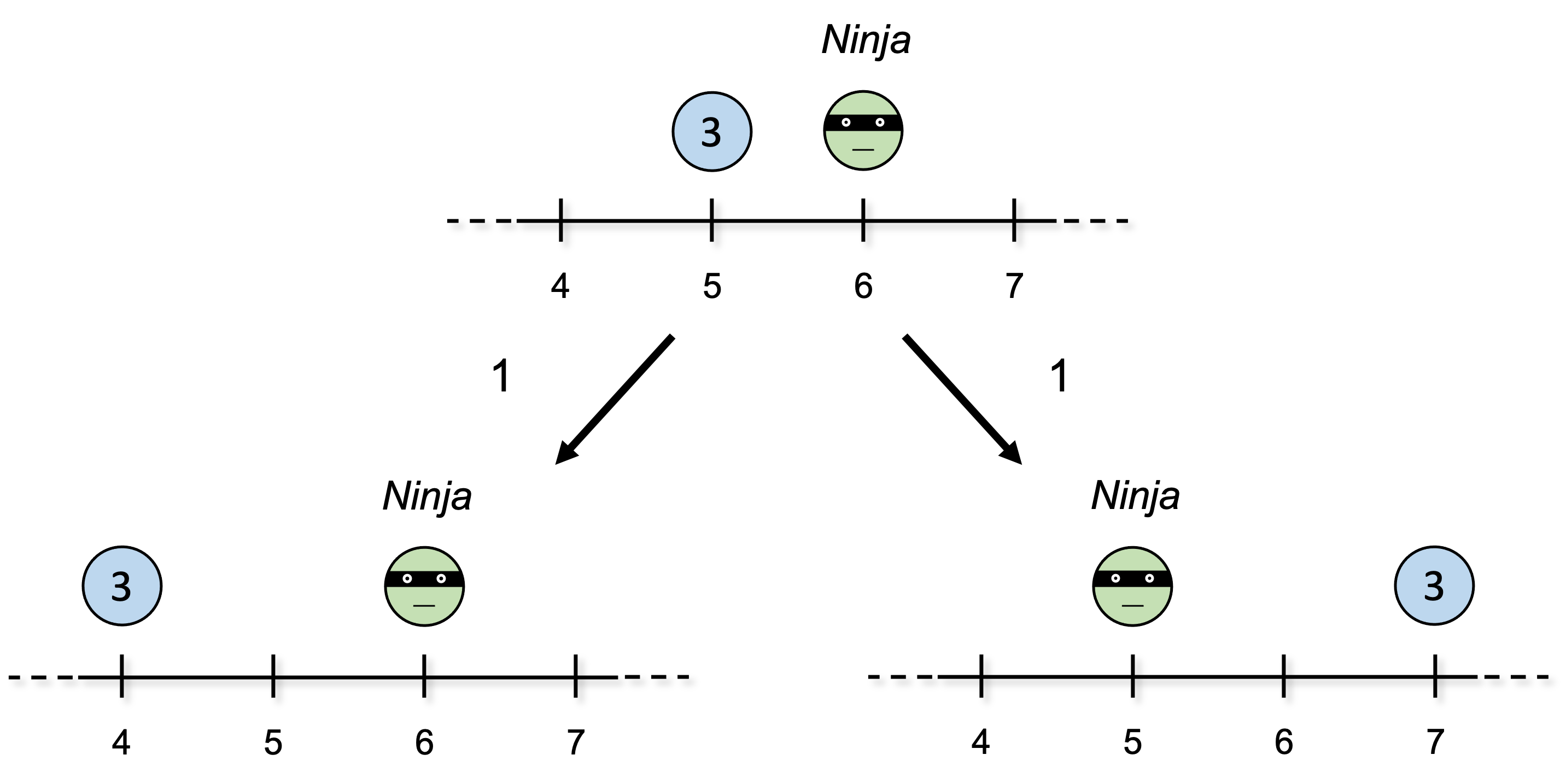
  Figure 5.

  

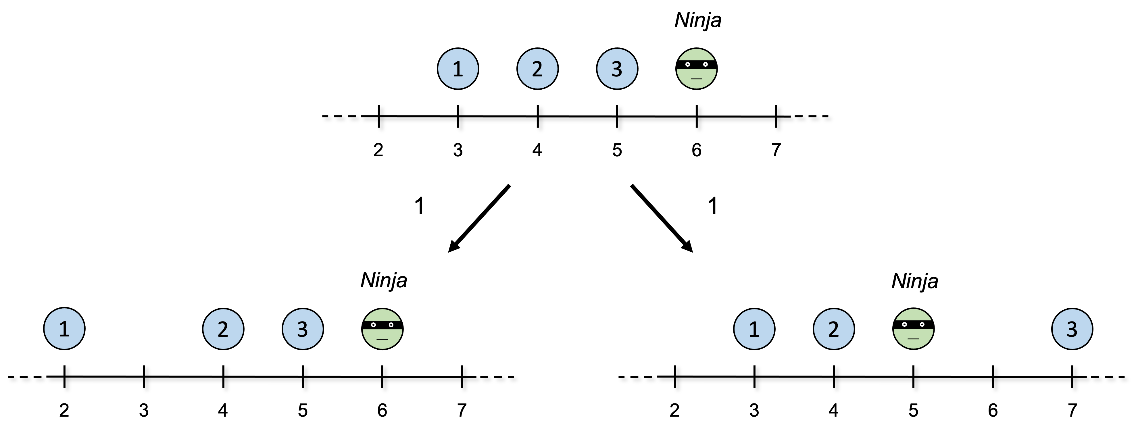
  Figure 6.

• (The Ninja returns) In the Ninja particle system, it is not allowed the situation in which the Ninja is at site $x\in\{N,0\}$ and one of the other particles is at $|x-1|$. If the Ninja is at $x\in\{N,0\}$, it can escape from the absorbing site $x\in\{N,0\}$ when one of the other particles tries to jump at $|x-1|$. Indeed suppose that $x_{i}=|x-2|$, then all other particles behave as simple symmetric random walks jumping at rate one, subject to the exclusion rule and with $\{0,N\}$ acting as absorbing sites, while the couple $(x_{i},\textit{Ninja})=(|x-2|,x)$ jumps at rate $1$ to

  $$\left(|x-2|-\frac{x-|x-2|}{2},x\right)$$

  if $|x-2|-\frac{x-|x-2|}{2}$ is empty and at rate $1$ to

  $$\left(x,x-\frac{x-|x-2|}{2}\right)$$

  (see Figure 7).

  

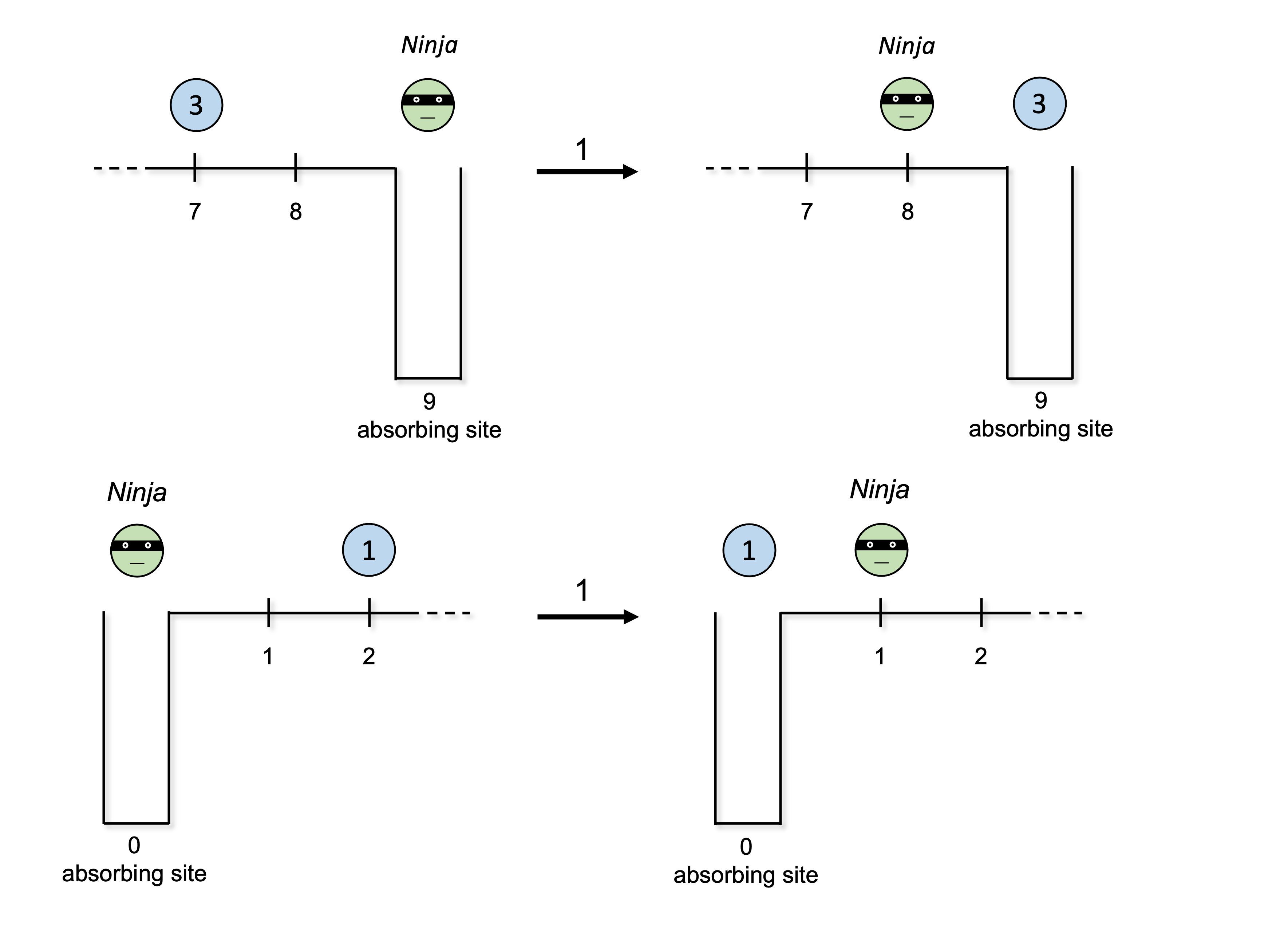
  Figure 7.

We now describe the dynamics of this particle system that we call Ninja-process via its generator

$$\hat{\mathcal{L}}^{\textit{Ninja}}=\hat{\mathcal{L}}^{\textit{Ninja}}_{1}+\hat{\mathcal{L}}^{\textit{Ninja}}_{2}+\hat{\mathcal{L}}^{\textit{Ninja}}_{3}$$

acting on functions $f:[N]^{k+1}\to{\mathbb{R}}$.

$\hat{\mathcal{L}}^{\textit{Ninja}}_{1}$ describes the dynamics in Case 1 and it is given by

$$\hat{\mathcal{L}}^{\textit{Ninja}}_{1}f(x_{1},\ldots,x_{k+1})=\left(\prod_{i=1}^{k}{{\bf 1}}_{\{|x_{i}-x_{k+1}|\neq 1\}}\right){{\bf 1}}_{\{x_{k+1}\notin\{0,N\}\}}$$

$$\times\left(\sum_{i=1}^{k+1}{{\bf 1}}_{\{x_{i}\notin\{0,N\}\}}\left(1-\sum_{j=1}^{k+1}{{\bf 1}}_{\{x_{j}=x_{i}\pm 1\}})\right)\right.$$

$$\qquad\left.\times(f(x_{1},\ldots,x_{i-1},x_{i}\pm 1,x_{i+1},\ldots,x_{k+1})-f(x_{1},\ldots,x_{k+1}))\right).$$

$\hat{\mathcal{L}}^{\textit{Ninja}}_{2}$ describes the dynamics in Case 2 (see Figure 5 and 6) and it is given by

$$\hat{\mathcal{L}}^{\textit{Ninja}}_{2}f(x_{1},\ldots,x_{k+1})=\left(1-\prod_{i=1}^{k}{{\bf 1}}_{\{|x_{i}-x_{k+1}|\neq 1\}}\right){{\bf 1}}_{\{x_{k+1}\notin\{0,N\}\}}$$

$$\times\left(\sum_{i=1}^{k}{{\bf 1}}_{\{x_{i}\notin\{0,N\}\}}\left[\left(1-\sum_{j=1}^{k+1}{{\bf 1}}_{\{x_{j}=x_{i}\pm 1\}})\right)\right.\right.$$

$$\qquad\left.\left.\times(f(x_{1},\ldots,x_{i-1},x_{i}\pm 1,x_{i+1},\ldots,x_{k+1})-f(x_{1},\ldots,x_{k+1}))\right.\right.$$

$$\left.\left.+{{\bf 1}}_{\{|x_{i}-x_{k+1}|=1\}}(1-\sum_{j=1}^{k+1}{{\bf 1}}_{\{x_{i}+2(x_{k+1}-x_{i})=x_{j}\}})\right.\right.$$

$$\left.\left.\times(f(x_{1},\ldots,x_{i-1},x_{i}+2(x_{k+1}-x_{i}),x_{i+1},\ldots,x_{i})-f(x_{1},\ldots,x_{k+1}))\right]\right).$$

$\hat{\mathcal{L}}^{\textit{Ninja}}_{3}$ describes the dynamics in Case 3 (see Figure 7) and it is given by

$$\hat{\mathcal{L}}^{\textit{Ninja}}_{3}f(x_{1},\ldots,x_{k})={{\bf 1}}_{\{x_{k+1}\in\{0,N\}\}}$$

$$\times\left(\sum_{i=1}^{k}{{\bf 1}}_{\{x_{i}\notin\{0,N\}\}}\left[{{\bf 1}}_{\{|x_{i}-x_{k+1}|\neq 2\}}\left(1-\sum_{j=1}^{k}{{\bf 1}}_{\{x_{j}=x_{i}\pm 1\}})\right)\right.\right.$$

$$\qquad\left.\left.\times(f(x_{1},\ldots,x_{i-1},x_{i}\pm 1,x_{i+1},\ldots,x_{k+1})-f(x_{1},\ldots,x_{k+1}))\right.\right.$$

$$\left.\left.+{{\bf 1}}_{\{|x_{i}-x_{k+1}|=2\}}(1-\sum_{j=1}^{k+1}{{\bf 1}}_{\{x_{i}-(x_{k+1}-x_{i})/2=x_{j}\}})\right.\right.$$

$$\left.\left.\times(f(x_{1},\ldots,x_{i-1},x_{i}-(x_{k+1}-x_{i})/2,x_{i+1},\ldots,x_{k+1})-f(x_{1},\ldots,x_{k+1}))\right.\right.$$

$$\left.\left.+{{\bf 1}}_{\{|x_{i}-x_{k+1}|=2\}}(f(x_{1},\ldots,x_{i-1},x_{k+1},x_{i+1},\ldots,x_{i}(x_{k+1}-x_{i})/2)-f(x_{1},\ldots,x_{k+1}))\right]\right).$$

4.2. Consequences of the construction and the coupling

From the construction of the Ninja-process, the two propositions below follow. The first one states that if one forgets the labels in the Ninja process and looks at the configuration process associated to it, then the usual dual boundary driven process on $[N]_{0}$ is observed.

Proposition 4.3.

Let $(X^{(1)}_{t},\ldots,X^{(k)}_{t},\textit{Ninja}_{t})_{t\geq 0}$ be the Ninja-process and define

$$\mathcal{N}^{[N]_{0}}_{t}:=\sum_{i=1}^{k}\delta_{X^{(i)}_{t}}+\delta_{\textit{Ninja}_{t}}.$$

Then, if $\xi^{[N]_{0}}_{0}=\sum_{i=1}^{k}\delta_{X^{(i)}_{0}}+\delta_{\textit{Ninja}_{0}}$,

$$(\mathcal{N}^{[N]_{0}}_{t})_{t\geq 0}=(\xi^{[N]_{0}}_{t})_{t\geq 0}$$

in distribution.

Proof.

The result follows from the fact the for all $G:[N]_{0}^{k+1}\to{\mathbb{R}}$ permutation invariant, i.e.

$$G(x_{1},\ldots,x_{k+1})=G\left(\sum_{i=1}^{k+1}\delta_{x_{i}}\right),$$

we have

$$\hat{\mathcal{L}}^{\textit{Ninja}}G=\hat{\mathcal{L}}^{[N]_{0}}G$$

which is easy to check by direct inspection.

Indeed notice that all the transitions in the Ninja-process occur at rate one.

Moreover, if $(x_{1},\ldots,x_{k+1})$ is such that

$$\left(\prod_{i=1}^{k}{{\bf 1}}_{\{|x_{i}-x_{k+1}|\neq 1\}}\right){{\bf 1}}_{\{x_{k+1}\notin\{0,N\}\}}=1,$$

i.e. we are in Case 1, then obviously

$$\hat{\mathcal{L}}^{\textit{Ninja}}_{1}G(x_{1},\ldots,x_{k+1})=\hat{\mathcal{L}}^{[N]_{0}}G(x_{1},\ldots,x_{k+1}).$$

If $(x_{1},\ldots,x_{k+1})$ is such that

$$\left(1-\prod_{i=1}^{k}{{\bf 1}}_{\{|x_{i}-x_{k+1}|\neq 1\}}\right){{\bf 1}}_{\{x_{k+1}\notin\{0,N\}\}}{{\bf 1}}_{\{x_{i}\notin\{0,N\}\}}=1,$$

and

$${{\bf 1}}_{\{|x_{i}-x_{k+1}|=1\}}(1-\sum_{j=1}^{k+1}{{\bf 1}}_{\{x_{i}+2(x_{k+1}-x_{i})=x_{j}\}})=1,$$

with, e.g. $x_{k+1}=x_{i}+1$, i.e. we are in Case 2 (see Figure 5 and 6), because the transition

$$(x_{1},\ldots,x_{k+1})\to(x_{1},\ldots,x_{i-1},x_{i}+2(x_{k+1}-x_{i}),x_{i+1},\ldots,x_{i})$$

corresponds to the configuration transition

$$\sum_{j=1}^{k+1}\delta_{x_{j}}\to\sum_{j=1}^{k+1}\delta_{x_{j}}-\delta_{x_{k+1}}+\delta_{x_{k+1}+1}$$

then

$$\hat{\mathcal{L}}^{\textit{Ninja}}_{2}G(x_{1},\ldots,x_{k+1})=\hat{\mathcal{L}}^{[N]_{0}}G\left(\sum_{i=1}^{k+1}\delta_{x_{i}}\right).$$

If $(x_{1},\ldots,x_{k+1})$ is such that

$${{\bf 1}}_{\{x_{k+1}\in\{0,N\}\}}{{\bf 1}}_{\{x_{i}\notin\{0,N\}\}}{{\bf 1}}_{\{|x_{i}-x_{k+1}|=2\}},$$

with, e.g., ${x_{k+1}}=N$ and thus $x_{i}=N-2$, i.e. we are in Case 3 (see Figure 7), because the transition

$$(x_{1},\ldots,x_{k+1})\to(x_{1},\ldots,x_{i-1},x_{k+1},x_{i+1},\ldots,x_{i}+(x_{k+1}-x_{i})/2)$$

corresponds to the configuration transition

$$\sum_{j=1}^{k+1}\delta_{x_{j}}\to\sum_{j=1}^{k+1}\delta_{x_{j}}-\delta_{N-2}+\delta_{N-1}$$

then

$$\hat{\mathcal{L}}^{\textit{Ninja}}_{3}G(x_{1},\ldots,x_{k+1})=\hat{\mathcal{L}}^{[N]_{0}}G\left(\sum_{i=1}^{k+1}\delta_{x_{i}}\right).$$

Because for all $\{x_{1},\ldots,x_{k+1}\}\in[N]_{0}$ such that $\sum_{i=1}^{k+1}\delta_{x_{i}}(x)\in\{0,1\}$ for all $x\in[N-1]$

$$\left(\prod_{i=1}^{k}{{\bf 1}}_{\{|x_{i}-x_{k+1}|\neq 1\}}\right){{\bf 1}}_{\{x_{k+1}\notin\{0,N\}\}}\\ +\left(1-\prod_{i=1}^{k}{{\bf 1}}_{\{|x_{i}-x_{k+1}|\neq 1\}}\right){{\bf 1}}_{\{x_{k+1}\notin\{0,N\}\}}+{{\bf 1}}_{\{x_{k+1}\in\{0,N\}\}}=1$$ (4.3)

the proof is concluded.

∎

The second one, provides a map from the Ninja-process to the dual of the boundary driven SSEP evolving on the reduced graph $[N-1]_{0}$ with $\{0,N-1\}$ acting as absorbing sites, namely to $(\xi^{[N-1]_{0}}_{t})_{t\geq 0}$.

Proposition 4.4.

For $x,y\in[N]_{0}$ set

$$\pi(x,y):=\begin{cases}N-1&\text{if }\ y=x=N\\ x-{\boldsymbol{1}}_{\{y<n\}}&\text{otherwise}.\end{cases}$$ (4.4)

Let $(X^{(1)}_{t},\ldots,X^{(k)}_{t},\textit{Ninja}_{t})_{t\geq 0}$ be the Ninja-process and define

$$\mathcal{N}^{[N-1]_{0}}_{t}:=\sum_{i=1}^{k}\delta_{\pi(X^{(i)}_{t},\textit{Ninja}_{t})}.$$

Then, if $\xi^{[N-1]_{0}}_{0}=\sum_{i=1}^{k}\delta_{\pi(X^{(i)}_{0},\textit{Ninja}_{0})}$,

$$(\mathcal{N}^{[N-1]_{0}}_{t})_{t\geq 0}=(\xi^{[N-1]_{0}}_{t})_{t\geq 0}$$

in distribution.

Proof.

Similarly to the proof of Proposition 4.3, the result follows from the fact the for all $G:[N]_{0}^{k}\to{\mathbb{R}}$ permutation invariant, i.e.

$$G(x_{1},\ldots,x_{k})=G\left(\sum_{i=1}^{k}\delta_{x_{i}}\right),$$

we have, for all $x_{1},\ldots,x_{k}$

$$\hat{\mathcal{L}}^{\textit{Ninja}}G(\pi(x_{1},x_{k+1}),\ldots,\pi(x_{k},x_{k+1}))=\hat{\mathcal{L}}^{[N]_{0}}G\left(\sum_{i=1}^{k}\delta_{x_{i}}\right)$$

for all $x_{k+1}\in[N]_{0}$ such that, if $x_{k+1}\notin\{0,N\}$, $\sum_{i=1}^{k}\delta_{x_{i}}(x_{k+1})=0.$

We do not provide all the details and we just point out that

• (see Figure 5 and 6) if $x_{k+1}=x_{i}+1$ the transition

  $$(x_{1},\ldots,x_{k+1})\to(x_{1},\ldots,x_{i-1},x_{i}+2(x_{k+1}-x_{i}),x_{i+1},\ldots,x_{i})$$

  in the Ninja-process, if allowed, corresponds to the transition

  $$\sum_{i=1}^{k}\delta_{\pi(x_{i},x_{k+1})}\to\sum_{i=1}^{k}\delta_{\pi(x_{i},x_{k+1})}-\delta_{x_{i}}+\delta_{x_{i}+1}$$

  in the $(\mathcal{N}^{[N-1]_{0}}_{t})_{t\geq 0}$ process.

• (see Figure 7) if ${x_{k}+1}=N$ and $x_{i}=N-2$, i.e. we are in Case 3,

  $$(x_{1},\ldots,x_{k+1})\to(x_{1},\ldots,x_{i-1},x_{k+1},x_{i+1},\ldots,x_{i}+(x_{k+1}-x_{i})/2)$$

  in the Ninja-process, corresponds to the transition

  $$\sum_{i=1}^{k}\delta_{\pi(x_{i},x_{k+1})}\to\sum_{i=1}^{k}\delta_{\pi(x_{i},x_{k+1})}-\delta_{N-2}+\delta_{N-1}$$

  in the $(\mathcal{N}^{[N-1]_{0}}_{t})_{t\geq 0}$ process and the particle at $N-1$ will stay there forever.

Both the above transitions are usual transitions in the dual BD-SSEP $(\xi^{[N-1]_{0}}_{t})_{t\geq 0}$. ∎

We conclude this section by collecting in the corollary below some direct consequences of Propositions 4.3 and 4.4 which will be used in the proof of Theorem 4.1. The result below follows from the observation that the function

$$f(x_{1},\ldots,x_{k}):={{\bf 1}}_{\{\left(\sum_{i=1}^{k}{{\bf 1}}_{\{x_{i}=N\}}\right)=k\}}$$

is permutation invariant.

Corollary 4.5.

1. For all $x_{1},\ldots,x_{k+1}\in[N]_{0}$ with

   $$1\leq x_{1}<\ldots<x_{k}\leq N$$

   and

   $$x_{k+1}\notin\{x_{1},\ldots,x_{k}\}$$

   $${\mathbb{P}}^{\textit{Ninja}}_{x_{1},\ldots,x_{k},x_{k+1}}(\{X^{(1)}_{\infty}=N,\ldots,X_{\infty}^{(k)}=N,\textit{Ninja}_{\infty}=N\})\\ =\hat{\mathbb{P}}^{[N]_{0}}_{\{x_{1},\ldots,x_{k+1}\}}(\xi^{[N]_{0}}_{\infty}(N)=k+1).$$ (4.5)

2. For each $1\leq x_{1}<\ldots<x_{k}\leq N-1$

   $${\mathbb{P}}^{\textit{Ninja}}_{x_{1},\ldots,x_{k},x_{k+1}}(\{X^{(1)}_{\infty}=N,\ldots,X_{\infty}^{(k)}=N\})\\ ={\mathbb{P}}^{\textit{Ninja}}_{x_{1},\ldots,x_{k},y_{k+1}}(\{X^{(1)}_{\infty}=N,\ldots,X_{\infty}^{(k)}=N\})=\hat{\mathbb{P}}^{[N-1]_{0}}_{\{x_{1},\ldots,x_{k}\}}(\xi^{[N-1]_{0}}_{\infty}(N-1)=k).$$ (4.6)

   for all $x_{k+1},y_{k+1}\in[N]_{0}\setminus\{x_{1},\ldots,x_{k}\}$.

4.3. Proof of Theorem 4.1

We now have almost all the elements to prove Theorem 4.1. Indeed by Corollary 4.5 we have that, for all $x_{k+1}\notin\{x_{1},\ldots,x_{k}\}$,

$$\hat{\mathbb{P}}^{[N-1]_{0}}_{\{x_{1},\ldots,x_{k}\}}(\xi^{[N-1]_{0}}_{\infty}(N-1)=k)=$$

$$={\mathbb{P}}^{\textit{Ninja}}_{x_{1},\ldots,x_{k},x_{k+1}}(\{X^{(1)}_{\infty}=N,\ldots,X_{\infty}^{(k)}=N,\textit{Ninja}_{\infty}=N\})$$

$$+\ {\mathbb{P}}^{\textit{Ninja}}_{x_{1},\ldots,x_{k},x_{k+1}}(\{X^{(1)}_{\infty}=N,\ldots,X_{\infty}^{(k)}=N,\textit{Ninja}_{\infty}=0\})$$

and denoting by $E$ be the event that all the $k$ particles are absorbed at $N$, i.e.

$$E:=\{X^{x_{i}}_{\infty}=N\ \forall i\in\{1,\ldots,k\}\}$$ (4.7)

we obtain

$$\hat{\mathbb{P}}^{[N-1]_{0}}_{\{x_{1},\ldots,x_{k}\}}(\xi^{[N-1]_{0}}_{\infty}(N-1)=k)=\hat{\mathbb{P}}^{[N]_{0}}_{\{x_{1},\ldots,x_{k+1}\}}(\xi^{[N]_{0}}_{\infty}(N)=k+1)\\ +{\mathbb{P}}^{\textit{Ninja}}_{x_{1},\ldots,x_{k},x_{k+1}}(\textit{Ninja}_{\infty}=0|E){\mathbb{P}}^{[N-1]_{0}}_{\{x_{1},\ldots,x_{k}\}}(\xi^{[N-1]_{0}}_{\infty}(N)=k).$$

The conclusion of the proof follows from the next proposition.

Proposition 4.6.

Let $(X^{(1)}_{t},\ldots,X^{(k)}_{t},\textit{Ninja}_{t})_{t\geq 0}$ be the Ninja-process and recall the event $E$ given in (4.7). Then, for all $x_{k+1}\notin\{x_{1},\ldots,x_{k}\}$,

$${\mathbb{P}}^{\textit{Ninja}}_{x_{1},\ldots,x_{k},x_{k+1}}(\textit{Ninja}_{\infty}=0|E)=1-\frac{x_{k+1}-k}{N}.$$ (4.8)

Proof.

We consider the skeleton chain

$$(X^{(1)}_{n},\ldots,X^{(k)}_{n},\textit{Ninja}_{n})_{n\in{\mathbb{N}}}$$

since we are interested in computing absorption probabilities only and we define by

$$(\bar{X}^{(1)}_{n},\ldots,\bar{X}^{(k)}_{n},\overline{\textit{Ninja}}_{n})_{n\in{\mathbb{N}}}$$

the Ninja process conditioned on the event $E$.

In order to compute the conditional probability on the left hand side of (4.8), we introduce the following auxiliary stochastic process:

$$\bar{M}_{n}:=N-\overline{\textit{Ninja}}_{n}+\sum_{\ell=1}^{k}{\boldsymbol{1}}_{\{\bar{X}^{(\ell)}_{n}<\overline{\textit{Ninja}}_{n}\}}.$$

First notice that, ${\mathbb{P}}^{\textit{Ninja}}_{x_{1},\ldots,x_{k},x_{k+1}}$-a.s.

$$\lim_{n\to\infty}\bar{M}_{n}=N\ {{\bf 1}}_{\{\overline{\textit{Ninja}}_{\infty}=0\}}.$$

Because $\bar{M}_{n}\leq N+k$ for each $n\in{\mathbb{N}}$, the dominated convergence theorem guarantees that

$$\lim_{n\to\infty}{\mathbb{E}}^{\textit{Ninja}}_{x_{1},\ldots,x_{k},x_{k+1}}[\bar{M}_{n}] =N\ {\mathbb{P}}^{\textit{Ninja}}_{x_{1},\ldots,x_{k},x_{k+1}}(\overline{\textit{Ninja}}_{\infty}=0)$$

$$=N\ {\mathbb{P}}^{\textit{Ninja}}_{x_{1},\ldots,x_{k},x_{k+1}}({\textit{Ninja}}_{\infty}=0|E).$$ (4.9)

We conclude by showing that for all $n\in{\mathbb{N}}$

$${\mathbb{E}}^{\textit{Ninja}}_{x_{1},\ldots,x_{k},x_{k+1}}[\bar{M}_{n}]=\bar{M}_{0}=N-x_{k+1}+k$$

from which the thesis follows.

It is enough to show that for all $x_{1},\ldots,x_{k+1}$

$${\mathbb{E}}^{\textit{Ninja}}_{x_{1},\ldots,x_{k},x_{k+1}}[\bar{M}_{1}]=N-x_{k+1}+k$$

since then, by the Markov property, we will show that the equality holds for all $n\in{\mathbb{N}}$.

For this purpose, we consider three different scenarios. The first one is when there exists exactly one $i$ such that $|x_{i}-x_{k+1}|=1$ or when $x_{i}=2$ and $x_{k+1}=0$ or when $x_{i}=N-2$ and $x_{k+1}=N$. In this case, if a particle with label $j\neq i$ jumps, the process will not change its value since each term in the sum composing $\bar{M}_{1}$ remains the same as in $\bar{M}_{0}$. If the $i$-th particle is at the left of the Ninja (the $k+1$ particle), i.e. $x_{k+1}-x_{i}=1$, then if it jumps to the left, no terms changes in $\bar{M}_{1}$, while if it jumps to the right interacting with the ninja then

$$\overline{\textit{Ninja}}_{1}-\overline{\textit{Ninja}}_{0}=-1$$

and

$${\boldsymbol{1}}_{\{\bar{X}^{x_{i}}_{1}<\overline{\textit{Ninja}}_{1}\}}-{\boldsymbol{1}}_{\{\bar{X}^{x_{i}}_{0}<\overline{\textit{Ninja}}_{0}\}}=-1$$

and thus $\bar{M}_{0}=\bar{M}_{1}$ for any possible transition. Similarly, one can deduce the same conclusions when $x_{i}-x_{k+1}=1$, or when $x_{i}=2$ and $x_{k+1}=0$ or when $x_{i}=N-2$ and $x_{k+1}=N$. The second one consists in the case where there exists $i$ and $j$ such that $x_{k+1}-x_{i}=1$ and $x_{j}-x_{k+1}=1$; then the Ninja cannot move and all the other particles cannot jump across the Ninja and thus $\bar{M}_{1}=\bar{M}_{0}$.

Finally the third scenario consists in the case $\min\{|x_{i}-x_{k+1}|,\ i\in\{1,\ldots,k\}\}\geq 2$ with $x_{k+1}\notin\{0,N\}$. In this case, no particle can jump across the Ninja in one step and thus

$$\sum_{i=1}^{k}{\boldsymbol{1}}_{\{\bar{X}^{(i)}_{1}<\overline{\textit{Ninja}}_{1}\}}=\sum_{i=1}^{k}{\boldsymbol{1}}_{\{\bar{X}^{(i)}_{0}<\overline{\textit{Ninja}}_{0}\}}.$$

However, in this case the Ninja can move both to the left and to the right. We now show that in this third case, despite the conditioning to the event $E$,

$${\mathbb{P}}^{\textit{Ninja}}_{x_{1},\ldots,x_{k},x_{k+1}}(\overline{\textit{Ninja}}_{1}=x_{k+1}+1)={\mathbb{P}}^{\textit{Ninja}}_{x_{1},\ldots,x_{k},x_{k+1}}(\overline{\textit{Ninja}}_{1}=x_{k+1}-1)$$

from which we conclude that

$${\mathbb{E}}^{\textit{Ninja}}_{x_{1},\ldots,x_{k},x_{k+1}}[\bar{M}_{1}]=\bar{M}_{0}.$$

Recall that by definition of the Ninja-process: the non-conditioned process satisfies

$${\mathbb{P}}^{\textit{Ninja}}_{x_{1},\ldots,x_{k},x_{k+1}}({\textit{Ninja}}_{1}=x_{k+1}+1)={\mathbb{P}}^{\textit{Ninja}}_{x_{1},\ldots,x_{k},x_{k+1}}({\textit{Ninja}}_{1}=x_{k+1}-1)$$

since in this case, the Ninja is performing a simple symmetric random walk. By Bayes theorem and the Markov property we have

$${\mathbb{P}}^{\textit{Ninja}}_{x_{1},\ldots,x_{k},x_{k+1}}(\overline{\textit{Ninja}}_{1}=x_{k+1}+1)={\mathbb{P}}^{\textit{Ninja}}_{x_{1},\ldots,x_{k},x_{k+1}}({\textit{Ninja}}_{1}=x_{k+1}+1|E)$$

$$=\frac{{\mathbb{P}}^{\textit{Ninja}}_{x_{1},\ldots,x_{k},x_{k+1}}(E|{\textit{Ninja}}_{1}=x_{k+1}+1)}{{\mathbb{P}}^{\textit{Ninja}}_{x_{1},\ldots,x_{k},x_{k+1}}(E)}{\mathbb{P}}^{\textit{Ninja}}_{x_{1},\ldots,x_{k},x_{k+1}}({\textit{Ninja}}_{1}=x_{k+1}+1)$$

$$=\frac{{\mathbb{P}}^{\textit{Ninja}}_{x_{1},\ldots,x_{k},x_{k+1}+1}(E)}{{\mathbb{P}}^{\textit{Ninja}}_{x_{1},\ldots,x_{k},x_{k+1}}(E)}{\mathbb{P}}^{\textit{Ninja}}_{x_{1},\ldots,x_{k},x_{k+1}}({\textit{Ninja}}_{1}=x_{k+1}+1).$$

By Corollary 4.6, we have that

$${\mathbb{P}}^{\textit{Ninja}}_{x_{1},\ldots,x_{k},x_{k+1}+1}(E)={\mathbb{P}}^{\textit{Ninja}}_{x_{1},\ldots,x_{k},x_{k+1}}(E)$$

concluding that

$${\mathbb{P}}^{\textit{Ninja}}_{x_{1},\ldots,x_{k},x_{k+1}}(\overline{\textit{Ninja}}_{1}=x_{k+1}+1)={\mathbb{P}}^{\textit{Ninja}}_{x_{1},\ldots,x_{k},x_{k+1}}({\textit{Ninja}}_{1}=x_{k+1}+1).$$

The same arguments gives

$${\mathbb{P}}^{\textit{Ninja}}_{x_{1},\ldots,x_{k},x_{k+1}}(\overline{\textit{Ninja}}_{1}=x_{k+1}-1)={\mathbb{P}}^{\textit{Ninja}}_{x_{1},\ldots,x_{k},x_{k+1}}({\textit{Ninja}}_{1}=x_{k+1}-1)$$

and thus

$${\mathbb{P}}^{\textit{Ninja}}_{x_{1},\ldots,x_{k},x_{k+1}}(\overline{\textit{Ninja}}_{1}=x_{k+1}+1)=P^{\textit{Ninja}}_{x_{1},\ldots,x_{k},x_{k+1}}(\overline{\textit{Ninja}}_{1}=x_{k+1}-1).$$

Finally, denoting by $(\bar{\mathcal{F}}_{n})_{n\in{\mathbb{N}}}$ the natural filtration generated by the conditioned process $(\bar{X}^{(1)}_{n},\ldots,\bar{X}^{(k)}_{n},\overline{\textit{Ninja}}_{n})_{n\in{\mathbb{N}}}$, we obtain, using the Markov property

$${\mathbb{E}}^{\textit{Ninja}}_{x_{1},\ldots,x_{k},x_{k+1}}[\bar{M}_{n}]={\mathbb{E}}^{\textit{Ninja}}_{x_{1},\ldots,x_{k},x_{k+1}}[{\mathbb{E}}^{\textit{Ninja}}_{x_{1},\ldots,x_{k},x_{k+1}}[\bar{M}_{n}|\bar{\mathcal{F}}_{n-1}]]$$

$$={\mathbb{E}}^{\textit{Ninja}}_{x_{1},\ldots,x_{k},x_{k+1}}[{\mathbb{E}}^{\textit{Ninja}}_{X^{(1)}_{n-1},\ldots,X^{(k)}_{n-1},Ninja^{x_{k+1}}_{n-1}}[\bar{M}_{1}]].$$

The above term is equal to

$$\sum_{y_{1},\ldots,y_{k+1}}{\mathbb{P}}^{\textit{Ninja}}_{x_{1},\ldots,x_{k},x_{k+1}}(\bar{X}^{(1)}_{n-1}=y_{1},\ldots,\bar{X}^{(k)}_{n-1}=y_{k},\overline{\textit{Ninja}}_{n-1}=y_{k+1}){\mathbb{E}}^{\textit{Ninja}}_{y_{1},\ldots,y_{k},y_{k+1}}[\bar{M}_{1}]$$

$$=\bar{M}_{0}\sum_{y_{1},\ldots,y_{k+1}}{\mathbb{P}}^{\textit{Ninja}}_{x_{1},\ldots,x_{k},x_{k+1}}(\bar{X}^{(1)}_{n-1}=y_{1},\ldots,\bar{X}^{(k)}_{n-1}=y_{k},\overline{\textit{Ninja}}_{n-1}=y_{k+1})=\bar{M}_{0}$$

and the proof is concluded. ∎

Acknowledgments

S.F. acknowledges financial support from the Engineering and Physical Sciences Research Council of the United Kingdom through the EPSRC Early Career Fellowship EP/V027824/1. S.F. and A.G.C. thank the Hausdorff Institute for Mathematics (Bonn) for its hospitality during the Junior Trimester Program Stochastic modelling in life sciences funded by the Deutsche Forschungsgemeinschaft (DFG, German Research Foundation) under Germany’s Excellence Strategy - EXC-2047/1 - 390685813. If the authors’ staying at HIM has been so pleasant, productive and full of nice workshops and seminars is in great extent thanks to Silke Steinert-Berndt and Tomasz Dobrzeniecki: the authors are extremely grateful to them. The authors thank Simona Villa for making the pictures and P. Gonçalves, M. Jara, F. Sau and G. Schütz for useful discussions and comments. S.F. thanks P. Gonçalves for her kind hospitality at the Instituto Superior Técnico in Lisbon during June 2023. This project has received funding from the European Research Council (ERC) under the European Union’s Horizon 2020 research and innovative programme (grant agreement n. 715734).

References

- [1] Bernardin, C., and Jiménez-Oviedo, B. Fractional Fick’s law for the boundary driven exclusion process with long jumps. ALEA 14, 1 (2017), 473–-501.
- [2] Bernardin, C., Gonçalves, P., and Jiménez-Oviedo, B. Slow to fast infinitely extended reservoirs for the symmetric exclusion process with long jumps. Markov Process. Relat. Fields 25, (2019), 217–-274.
- [3] Bernardin, C., Cardoso, P., Gonçalves, P., and Scotta, S. Hydrodynamic limit for a boundary driven super-diffusive symmetric exclusion. (2020), arXiv preprint arXiv:2007.01621.
- [4] Bertini, L., De Sole, A., Gabrielli, D., Jona-Lasinio, G., and Landim, C. Stochastic interacting particle systems out of equilibrium. J. Stat. Mech., (2007), P07014.
- [5] Bertini, L., De Sole, A., Gabrielli, D., Jona-Lasinio, G., and Landim, C. Macroscopic fluctuation theory. Rev. Modern Phys. 87, 2 (2015), 593–636.
- [6] Carinci, G., Giardinà, C., Giberti, C., and Redig, F. Duality for stochastic models of transport. J. Stat. Phys. 152, 4 (2013), 657–697.
- [7] Carinci, G., Giardinà, C., and Redig, F. Consistent particle systems and duality. Electron. J. Probab. 26, (2021), 1–31.
- [8] Dello Schiavo, L., Portinale, L., and Sau, F. Scaling Limits of Random Walks, Harmonic Profiles, and Stationary Non-Equilibrium States in Lipschitz Domains. arXiv:2112.14196 (2021).
- [9] De Masi, A., Presutti, E. Mathematical Methods for Hydrodynamic Limits, 1501 of Lecture Notes in Mathematics. Springer-Verlag, Berlin, 1991.
- [10] Derrida, B., Evans, M. R., Hakim, V., and Pasquier, V. Exact solution of a D asymmetric exclusion model using a matrix formulation. J. Phys. A 26, 7 (1993), 1493–1517.
- [11] Derrida, B., Lebowitz, J. L., and Speer, E. R. Entropy of open lattice systems. J. Stat. Phys. 126, 4-5 (2007), 1083–1108.
- [12] Derrida, B., Lebowitz, J. L., and Speer, E. R. Large deviation of the density profile in the steady state of the open symmetric simple exclusion process. J. Stat. Phys. 107, (2007), 599–634.
- [13] Floreani, S., Redig, F., and Sau, F.. Orthogonal polynomial duality of boundary driven particle systems and non-equilibrium correlations. Ann. Inst. Henri Poincaré Probab. Stat. 58, 1 (2022), 220–247.
- [14] Franceschini, C., Frassek, R. and, Giardinà, C. Integrable heat conduction model J. Math. Phys. 64, 4 (2024), 043304.
- [15] Frassek, R. Eigenstates of triangularisable open XXX spin chains and closed-form solutions for the steady state of the open SSEP. J. Stat. Mech. 2005, (2020), 053104.
- [16] Frassek, R. and, Giardinà, C. Exact solution of an integrable non-equilibrium particle system. J. Math. Phys. 63, (2022), 103301.
- [17] Gantert, N., Nestoridi, E., and Schmid, D. Mixing times for the simple exclusion process with open boundaries. Ann. Appl. Probab. 33, 2 (2023), 1172–1212.
- [18] Gilbert, T. Heat conduction and the nonequilibrium stationary states of stochastic energy exchange processes. J. Stat. Mech. Theory Exp., 8 (2017), 083205, 27.
- [19] Gonçalves, P. Hydrodynamics for Symmetric Exclusion in Contact with Reservoirs. In Stochastic Dynamics Out of Equilibrium, G. Giacomin, S. Olla, E. Saada, H. Spohn, and G. Stoltz eds., Cham, 2019. Springer International Publishing.
- [20] Gonçalves, P., Jara, M., Menezes, O., and Neumann, A. Non-equilibrium and stationary fluctuations for the SSEP with slow boundary. Stochastic Process. Appl. 130, 7 (2020), 4326–4357.
- [21] Gonçalves, P., and Scotta, S. Diffusive to super-diffusive behavior in boundary driven exclusion. Markov Process. Relat. Fields 28, (2022), 149–-178.
- [22] Kipnis, C., Marchioro, C., and Presutti, E. Heat flow in an exactly solvable model. J. Stat. Phys. 27, 1 (1982), 65–74.
- [23] Landim, C., Milanés, A., and Olla, S. Stationary and nonequilibrium fluctuations in boundary driven exclusion processes. Markov Process. Related Fields 14, 2 (2008), 165–184.
- [24] Liggett, T. M. Stochastic Interacting Systems: Contact, Voter and Exclusion Processes, vol. 324 of Grundlehren der mathematischen Wissenschaften. Springer Berlin Heidelberg, Berlin, Heidelberg, 1999.
- [25] Liggett, T. M. Interacting particle systems. Classics in Mathematics. Springer-Verlag, Berlin, 2005. Reprint of the 1985 original.
- [26] Mallick, K. The exclusion process: A paradigm for non-equilibrium behaviour. Phys. A: Stat. Mech. Appl. 418, 2 (2015), 17–48.
- [27] Nándori, P. Local equilibrium in inhomogeneous stochastic models of heat transport. J. Stat. Phys. 164, 2 (2016), 410–437.
- [28] Salez, J. Universality of cutoff for exclusion with reservoirs. Ann. Probab. 51, 2 (2023), 478–494.
- [29] Schütz, G.M. Exactly solvable models for many-body systems far from equilibrium. In Phase transitions and critical phenomena vol. 19, C. Domb and J. Lebowitz eds., Academic Press, 2001.
- [30] Schütz, G.M. A reverse duality for the ASEP with open boundaries. Phys. A: Math. Theor., 56 (2023), 274001.
- [31] Spohn, H. Long range correlations for stochastic lattice gases in a nonequilibrium steady state. J. Phys. A 16, (1983), 4275–-4291.