On the two-loop BSM corrections to $h\longrightarrow\gamma\gamma$

in the aligned THDM

Giuseppe Degrassi${}^{\,a}$ and Pietro Slavich${}^{\,b}$

^a Dipartimento di Matematica e Fisica, Università di Roma Tre,

and INFN, Sezione di Roma Tre, I-00146 Rome, Italy.

^b Sorbonne Université, CNRS, Laboratoire de Physique Théorique et Hautes Energies,

LPTHE, F-75005, Paris, France.

1 Introduction

The discovery of a Higgs boson with mass around $125$ GeV and properties compatible with the predictions of the Standard Model (SM) [1, 2, 3, 4], combined with the negative (so far) results of the searches for additional new particles at the LHC, point to scenarios with at least a mild hierarchy between the electroweak (EW) scale and the scale of beyond-the-SM (BSM) physics. This said, the existence of new particles with masses around or even below the TeV scale, which could still be discovered in the current or future runs of the LHC, is not conclusively ruled out. This is especially the case if those new particles are colorless, and there is some mechanism that forbids or at least suppresses their mixing with the SM-like Higgs boson.

The Two-Higgs-Doublet Model (THDM) is one of the simplest and best-studied extensions of the SM (for reviews see, e.g., refs. [5, 6, 7]). In the CP-conserving versions of the model, the Higgs sector includes five physical states: two CP-even scalars, $h$ and $H$; one CP-odd scalar, $A$; and two charged scalars, $H^{\pm}$. As discussed, e.g., in ref. [8], the so-called “alignment” condition – in which one of the CP-even scalars has SM-like couplings to fermions and gauge bosons – can be realized through decoupling, when all of the other Higgs bosons are much heavier, or without decoupling, when a specific configuration of parameters in the Lagrangian suppresses the mixing between the SM-like scalar and the other CP-even scalar. If the THDM is embedded in a more-complicated extension of the SM that predicts the values of the quartic Higgs couplings, as is the case in supersymmetric models, the alignment condition can arise at the tree level from an underlying symmetry (see, e.g., ref. [9]), or it can result from cancellations between the tree-level couplings and their radiative corrections (see, e.g., ref. [10]). In contrast, when the THDM is treated as a stand-alone extension of the SM, the alignment condition can be enforced “from the bottom up”, based on the empirical observation that the couplings of the $125$-GeV Higgs boson appear to be essentially SM-like.

Beyond the requirement that they allow for a scalar with mass around $125$ GeV and SM-like couplings to fermions and gauge bosons, the quartic Higgs couplings of the THDM are subject to a number of experimental constraints from EW precision observables and flavor physics, as well as theory-driven constraints from perturbative unitarity and the stability of the scalar potential. Nevertheless, couplings of ${\cal O}(1$–$10)$ are still allowed by all constraints (see, e.g., refs. [11, 12]), and may even be favored (see, e.g., ref. [13]) if the THDM is to accommodate recent experimental anomalies such as the new CDF measurement of the $W$ mass [14]. Couplings in this range may induce sizable radiative corrections to the THDM predictions for physical observables, up to the point where one might wonder whether, in any given calculation, the uncomputed higher-order effects spoil the accuracy of the prediction. This has motivated a number of recent studies in which radiative corrections involving the quartic Higgs couplings of the THDM have been computed at the two-loop level. In particular, the two-loop corrections to the $\rho$ parameter have been computed in refs. [15, 16], various effects of the two-loop corrections to the scalar mass matrices have been examined in ref. [17], and the two-loop corrections to the trilinear self-coupling of the SM-like Higgs boson, $\lambda_{hhh}$, have been computed in refs. [18, 19]. In all cases it was found that the two-loop corrections can significantly modify the one-loop predictions, and should be taken into account for a precise determination of the considered observable.

In this paper we compute the dominant two-loop corrections to the decay width for the process $h\longrightarrow\gamma\gamma$ in the aligned THDM. Since the signal strength for this channel is currently measured with an accuracy of about $6\%$ [20], the requirement that the BSM contributions do not spoil the agreement with the theoretical prediction can put significant constraints on the parameter space of the THDM (see, e.g., ref. [21]). Once again, the possible presence of couplings of ${\cal O}(1$–$10)$ in the THDM Lagrangian motivates the calculation of $\Gamma[h\rightarrow\gamma\gamma]$ beyond the leading order (LO), which, for this observable, means beyond the one-loop level.

In the calculation of the two-loop BSM contributions to $\Gamma[h\rightarrow\gamma\gamma]$ we adopt the same simplifying assumptions as in the calculation of the $\rho$ parameter in refs. [15, 16]. In particular, we restrict our calculation to the CP-conserving THDM in the alignment limit; we work in the so-called “gaugeless limit” of vanishing EW gauge couplings, considering only the corrections that depend on the quartic Higgs couplings and possibly on the top Yukawa coupling; finally, we treat the mass of the SM-like scalar $h$ as negligible w.r.t. the masses of the BSM scalars, $H$, $A$ and $H^{\pm}$, and of the top quark. In order to obtain compact formulas for the two-loop corrections to the decay width, we make use of a low-energy theorem (LET) which connects them to the derivative of the photon self-energy w.r.t. the vacuum expectation value (vev) of the SM-like Higgs field [22, 23]. However, we also cross-check our result via a direct calculation of the $h\gamma\gamma$ amplitude. We note that care must be devoted to the definition of the alignment and vanishing-Higgs-mass conditions beyond LO, as well as to the avoidance of infrared (IR)-divergent contributions from diagrams involving massless particles.

The rest of the article is organized as follows: in section 2 we fix our notation for the Higgs sector of the THDM and discuss the renormalization of the scalar masses and mixing; in section 3 we outline our calculation of the dominant two-loop corrections to the decay width for $h\longrightarrow\gamma\gamma$; in section 4 we briefly discuss the numerical impact of the newly-computed corrections; section 5 contains our conclusions; finally, two appendices collect explicit formulas for the one-loop self-energies and tadpoles of the Higgs bosons and for the BSM part of the two-loop self-energy of the photon.

2 The Higgs sector of the aligned THDM

We start this section by describing the tree-level scalar potential and the Higgs mass spectrum of the THDM in the alignment limit. Note that we do not need to distinguish between different THDM “types” according to the form of their Higgs–fermion interactions, because in our calculation of the two-loop corrections to $\Gamma[h\rightarrow\gamma\gamma]$ we neglect all Yukawa couplings except the one of the top quark. We follow up by discussing the renormalization of the Higgs sector of the aligned THDM, in a “naive” approach that is justified by the simplifying assumptions adopted in our calculation.

2.1 The scalar potential, masses and mixing at the tree level

We consider a version of the THDM where flavor-changing neutral-current interactions are forbidden at the tree level by a $Z_{2}$ symmetry, softly broken by an off-diagonal mass term. In the so-called standard basis where this $Z_{2}$ symmetry applies, the scalar potential can be parametrized as

$$V_{0} = m_{11}^{2}\Phi_{1}^{\dagger}\Phi_{1}~{}+~{}m_{22}^{2}\Phi_{2}^{\dagger}\Phi_{2}~{}-~{}m_{12}^{2}\,\left(\Phi_{1}^{\dagger}\Phi_{2}~{}+~{}{\rm h.c.}\right)\,+~{}\frac{\lambda_{1}}{2}\,\left(\Phi_{1}^{\dagger}\Phi_{1}\right)^{2}\,+~{}\frac{\lambda_{2}}{2}\,\left(\Phi_{2}^{\dagger}\Phi_{2}\right)^{2}$$ (1)

$$+~{}\lambda_{3}\,\Phi_{1}^{\dagger}\Phi_{1}\,\Phi_{2}^{\dagger}\Phi_{2}~{}+~{}\lambda_{4}\,\Phi_{1}^{\dagger}\Phi_{2}\,\Phi_{2}^{\dagger}\Phi_{1}~{}+~{}\frac{\lambda_{5}}{2}\,\left[\left(\Phi_{1}^{\dagger}\Phi_{2}\right)^{2}+~{}{\rm h.c.}\right]~{},$$

where all of the masses and quartic couplings are assumed to be real to ensure CP conservation. We decompose the two $SU(2)$ doublets as

$$\Phi_{k}~{}=~{}\frac{1}{\sqrt{2}}\left(\!\begin{array}[]{c}\sqrt{2}\,\phi^{+}_{k}\\ v_{k}+\phi^{0}_{k}+i\,a_{k}\end{array}\!\right)~{}~{}~{}~{}~{}(k=1,2)~{},$$ (2)

where the two (real) vevs are related by $v_{1}^{2}+v_{2}^{2}=v^{2}$, with $v\approx 246$ GeV, and we define $\tan\beta\equiv v_{2}/v_{1}$. The minimum conditions for the scalar potential can be used to replace the mass parameters $m_{11}^{2}$ and $m_{22}^{2}$ with combinations of the remaining parameters in eq. (1) and the vevs:

$$m_{11}^{2} = m_{12}^{2}\,\tan\beta-\frac{v^{2}}{2}\,\left(\lambda_{1}\,c_{\beta}^{2}+\lambda_{345}\,s_{\beta}^{2}\right)~{},$$ (3)

$$m_{22}^{2} = m_{12}^{2}\,\cot\beta-\frac{v^{2}}{2}\,\left(\lambda_{2}\,s_{\beta}^{2}+\lambda_{345}\,c_{\beta}^{2}\right)~{},$$ (4)

where we introduced the shortcuts $c_{\theta}\equiv\cos\theta$ and $s_{\theta}\equiv\sin\theta$ for a generic angle $\theta$, and defined $\lambda_{345}\equiv\lambda_{3}+\lambda_{4}+\lambda_{5}$. The mass matrices for the pseudoscalar and charged components of the two doublets are diagonalized by the angle $\beta$:

$$\left(\!\begin{array}[]{c}G^{0}\\ A\end{array}\!\right)~{}=~{}R(\beta)\,\left(\!\begin{array}[]{c}a_{1}\\ a_{2}\end{array}\!\right)~{},~{}~{}~{}~{}~{}\left(\!\begin{array}[]{c}G^{+}\\ H^{+}\end{array}\!\right)~{}=~{}R(\beta)\,\left(\!\begin{array}[]{c}\phi_{1}^{+}\\ \phi_{2}^{+}\end{array}\!\right)~{},$$ (5)

where we defined

$$R(\theta)~{}\equiv~{}\left(\!\begin{array}[]{rr}c_{\theta}&\!s_{\theta}\\ -s_{\theta}&\!c_{\theta}\end{array}\!\right)~{},$$ (6)

and using the minimum conditions from eqs. (3) and (4) we get the tree-level masses

$$m^{2}_{G^{0}}=m^{2}_{G^{\pm}}=0~{},~{}~{}~{}m_{A}^{2}=M^{2}\,-\,\lambda_{5}\,v^{2}~{},~{}~{}~{}m_{H^{\pm}}^{2}=M^{2}\,-\,\frac{1}{2}(\lambda_{4}+\lambda_{5})\,v^{2}~{},$$ (7)

where we defined $M^{2}\equiv m_{12}^{2}/(s_{\beta}c_{\beta})$. The mass matrix for the neutral scalar components of the two doublets is instead diagonalized by an angle $\alpha$:

$$\left(\!\begin{array}[]{c}H\\ h\end{array}\!\right)~{}=~{}R(\alpha)\,\left(\!\begin{array}[]{c}\phi^{0}_{1}\\ \phi^{0}_{2}\end{array}\!\right)~{},$$ (8)

and the alignment condition in which the lighter mass eigenstate $h$ has SM-like couplings to fermions and gauge bosons corresponds to $\alpha=\beta-\pi/2$. To discuss this condition and its eventual renormalization, it is convenient to rotate the original Higgs doublets to the so-called Higgs basis:

$$\left(\!\begin{array}[]{c}\Phi_{{\rm{\scriptscriptstyle SM}}}\\ \Phi_{{\rm{\scriptscriptstyle BSM}}}\end{array}\!\right)~{}=~{}R(\beta)\,\left(\!\begin{array}[]{c}\Phi_{1}\\ \Phi_{2}\end{array}\!\right)~{},$$ (9)

in which one of the doublets develops the full SM-like vev $v$ and the other has vanishing vev:

$$\Phi_{\rm{\scriptscriptstyle SM}}~{}=~{}\left(\!\begin{array}[]{c}G^{+}\\ \frac{1}{\sqrt{2}}(v+\phi^{0}_{\rm{\scriptscriptstyle SM}}+i\,G^{0})\end{array}\!\right)~{},~{}~{}~{}~{}~{}\Phi_{\rm{\scriptscriptstyle BSM}}~{}=~{}\left(\!\begin{array}[]{c}H^{+}\\ \frac{1}{\sqrt{2}}(\phi^{0}_{\rm{\scriptscriptstyle BSM}}+i\,A)\end{array}\!\right)~{}.$$ (10)

The scalar potential in the Higgs basis becomes

$$V_{0} = M_{11}^{2}\,\Phi_{\rm{\scriptscriptstyle SM}}^{\dagger}\Phi_{\rm{\scriptscriptstyle SM}}~{}+~{}M_{22}^{2}\,\Phi_{\rm{\scriptscriptstyle BSM}}^{\dagger}\Phi_{\rm{\scriptscriptstyle BSM}}~{}-~{}M_{12}^{2}\,\left(\Phi_{\rm{\scriptscriptstyle SM}}^{\dagger}\Phi_{\rm{\scriptscriptstyle BSM}}~{}+~{}{\rm h.c.}\right)$$ (11)

$$+~{}\frac{\Lambda_{1}}{2}\,\left(\Phi_{\rm{\scriptscriptstyle SM}}^{\dagger}\Phi_{\rm{\scriptscriptstyle SM}}\right)^{2}\,+~{}\frac{\Lambda_{2}}{2}\,\left(\Phi_{\rm{\scriptscriptstyle BSM}}^{\dagger}\Phi_{\rm{\scriptscriptstyle BSM}}\right)^{2}$$

$$+~{}\Lambda_{3}\,\left(\Phi_{\rm{\scriptscriptstyle SM}}^{\dagger}\Phi_{\rm{\scriptscriptstyle SM}}\right)\left(\Phi_{\rm{\scriptscriptstyle BSM}}^{\dagger}\Phi_{\rm{\scriptscriptstyle BSM}}\right)+~{}\Lambda_{4}\,\left(\Phi_{\rm{\scriptscriptstyle SM}}^{\dagger}\Phi_{\rm{\scriptscriptstyle BSM}}\right)\left(\Phi_{\rm{\scriptscriptstyle BSM}}^{\dagger}\Phi_{\rm{\scriptscriptstyle SM}}\right)$$

$$+~{}\left[\,\frac{\Lambda_{5}}{2}\,\left(\Phi_{\rm{\scriptscriptstyle SM}}^{\dagger}\Phi_{\rm{\scriptscriptstyle BSM}}\right)^{2}+\,\left(\Lambda_{6}\,\Phi_{\rm{\scriptscriptstyle SM}}^{\dagger}\Phi_{\rm{\scriptscriptstyle SM}}\,+\,\Lambda_{7}\,\Phi_{\rm{\scriptscriptstyle BSM}}^{\dagger}\Phi_{\rm{\scriptscriptstyle BSM}}\right)\,\Phi_{\rm{\scriptscriptstyle SM}}^{\dagger}\Phi_{\rm{\scriptscriptstyle BSM}}~{}+~{}{\rm h.c.}\right]~{}.$$

The general relations between the parameters in eq. (11) and the analogous parameters in the standard basis, eq. (1), are given, e.g., in the appendix of ref. [24]. We list here the ones that will be relevant to the discussion that follows, specialized to the case of the $Z_{2}$-symmetric THDM:

$$M_{11}^{2} = m_{11}^{2}\,c_{\beta}^{2}+m_{22}^{2}\,s_{\beta}^{2}-m_{12}^{2}\,s_{2\beta}~{},$$ (12)

$$M_{22}^{2} = m_{11}^{2}\,s_{\beta}^{2}+m_{22}^{2}\,c_{\beta}^{2}+m_{12}^{2}\,s_{2\beta}~{},$$ (13)

$$M_{12}^{2} = \frac{1}{2}\,\left(m_{11}^{2}-m_{22}^{2}\right)\,s_{2\beta}+m_{12}^{2}\,c_{2\beta}~{},$$ (14)

$$\Lambda_{1} = \lambda_{1}\,c_{\beta}^{4}\,+\,\lambda_{2}\,s_{\beta}^{4}+\frac{1}{2}\,\lambda_{345}\,s_{2\beta}^{2}~{},$$ (15)

$$\Lambda_{6} = -\frac{1}{2}\,s_{2\beta}\,\left(\lambda_{1}\,c_{\beta}^{2}-\lambda_{2}\,s_{\beta}^{2}-\lambda_{345}\,c_{2\beta}\right)~{}.$$ (16)

The minimum conditions for the scalar potential become

$$M_{11}^{2}~{}=~{}-\frac{\Lambda_{1}}{2}\,v^{2}~{},~{}~{}~{}~{}M_{12}^{2}~{}=~{}\frac{\Lambda_{6}}{2}\,v^{2}~{},$$ (17)

and the mass parameter for the BSM doublet in eq. (13) can be rewritten as

$$M_{22}^{2}~{}=~{}M^{2}\,-\,\frac{1}{2}\,\left(\Lambda_{1}\,+\,2\,\cot 2\beta\,\Lambda_{6}\right)\,v^{2}~{}.$$ (18)

In the Higgs basis the tree-level mass matrices for the pseudoscalar and charged components of the two doublets are already diagonal, and the tree-level mass matrix for the neutral scalar components is given by

$$V~{}\supset~{}\frac{1}{2}\,\left(\phi^{0}_{\rm{\scriptscriptstyle SM}}~{}~{}~{}\phi^{0}_{\rm{\scriptscriptstyle BSM}}\right)~{}{\cal M}_{0}^{2}~{}\left(\!\begin{array}[]{c}\phi^{0}_{\rm{\scriptscriptstyle SM}}\\ \phi^{0}_{\rm{\scriptscriptstyle BSM}}\end{array}\!\right)~{},~{}~{}~{}~{}~{}~{}~{}~{}~{}{\cal M}_{0}^{2}=\left(\!\begin{array}[]{cc}\Lambda_{1}\,v^{2}&\Lambda_{6}\,v^{2}\\ \Lambda_{6}\,v^{2}&M^{2}\,+\,\widetilde{\Lambda}\,v^{2}\end{array}\right)~{},$$ (19)

where $\widetilde{\Lambda}\,=\,(\lambda_{1}+\lambda_{2}-2\lambda_{345})\,s_{2\beta}^{2}/4$ . It is then clear that, at the tree level, the alignment condition corresponds to $\Lambda_{6}=0$. When that is the case, the masses of the lighter and heavier neutral scalar reduce to

$$m_{h}^{2}~{}\rightarrow~{}\Lambda_{1}\,v^{2}~{},~{}~{}~{}~{}~{}~{}m_{H}^{2}~{}\rightarrow~{}M^{2}\,+\,\widetilde{\Lambda}\,v^{2}~{},$$ (20)

where we used arrows to indicate that the relations holds only in the alignment limit. Similarly, eq. (18) reduces to

$$M_{22}^{2}~{}\rightarrow~{}M^{2}\,-\,\frac{m_{h}^{2}}{2}~{},$$ (21)

and two of the quartic couplings of the standard basis can be traded for combinations of the remaining parameters:

$$\lambda_{1}~{}\rightarrow~{}-\lambda_{345}\,\tan^{2}\beta\,+\,\frac{m_{h}^{2}}{v^{2}\,c_{\beta}^{2}}~{},~{}~{}~{}~{}~{}\lambda_{2}~{}\rightarrow~{}-\lambda_{345}\,\cot^{2}\beta\,+\,\frac{m_{h}^{2}}{v^{2}\,s_{\beta}^{2}}~{},$$ (22)

which implies $m^{2}_{H}\rightarrow M^{2}+m_{h}^{2}-\lambda_{345}\,v^{2}$. We remark that the approximation of vanishing $m_{h}$, which we will adopt in section 3 to simplify our two-loop results, has to be understood here as $\Lambda_{1}\approx 0$ rather than $v\approx 0$, i.e., it amounts to a condition on the couplings entering eq. (15). Finally, we note that the combination of eqs. (8) and (9) implies

$$\left(\!\begin{array}[]{c}H\\ h\end{array}\!\right)~{}=~{}R(\alpha-\beta)\,\left(\!\begin{array}[]{c}\phi^{0}_{\rm{\scriptscriptstyle SM}}\\ \phi^{0}_{\rm{\scriptscriptstyle BSM}}\end{array}\!\right)~{},$$ (23)

thus, when $\alpha=\beta-\pi/2$ we get $h\rightarrow\phi^{0}_{\rm{\scriptscriptstyle SM}}$ and $H\rightarrow-\phi^{0}_{\rm{\scriptscriptstyle BSM}}$.

2.2 Mass and mixing renormalization

The calculation of two-loop corrections to $\Gamma[h\rightarrow\gamma\gamma]$ requires one-loop definitions for the parameters entering the LO prediction, which is itself at the one-loop level. The full one-loop renormalization of the Higgs sector of the THDM has been extensively studied in the literature [25, 26, 27, 28], and it involves a number of subtleties concerning the possible gauge dependence of the renormalized mixing angles. However, the simplifying assumptions that we adopt in our calculation (namely, alignment condition, vanishing SM-like Higgs mass $m_{h}$, and vanishing EW gauge couplings) allow us to bypass most of the complications discussed in those earlier studies. What we will ultimately need in the computation of the two-loop BSM corrections to $\Gamma[h\rightarrow\gamma\gamma]$ is the renormalization of the charged-Higgs mass $m_{H^{\pm}}$ and of the parameters $v$, $m_{12}^{2}$ and $\beta$ (the latter two make up $M^{2}$), taking care that the alignment and vanishing-$m_{h}$ conditions hold at the perturbative level considered in our calculation.

Beyond the tree level, the minimum conditions of the scalar potential in eq. (17) become

$$M_{11}^{2}~{}=~{}-\frac{\Lambda_{1}}{2}\,v^{2}~{}-~{}\frac{T_{\phi_{\rm{\scriptscriptstyle SM}}^{0}}}{v}~{},~{}~{}~{}~{}~{}~{}~{}M_{12}^{2}~{}=~{}\frac{\Lambda_{6}}{2}\,v^{2}~{}+~{}\frac{T_{\phi_{\rm{\scriptscriptstyle BSM}}^{0}}}{v}~{},$$ (24)

where $M^{2}_{11}$, $M^{2}_{12}$, $\Lambda_{1}$, $\Lambda_{6}$ and $v$ are now interpreted as $\overline{\rm MS}$-renormalized parameters at some scale $Q$. Note that eqs. (12)–(16) imply that the masses and quartic couplings in the standard basis, as well as the angle $\beta$, are also interpreted as $\overline{\rm MS}$-renormalized parameters. The quantities $T_{\varphi}$ in eq. (24) denote the finite parts of the one-loop tadpole diagrams  for the fields $\varphi=(\phi_{\rm{\scriptscriptstyle SM}}^{0},\phi_{\rm{\scriptscriptstyle BSM}}^{0}$). The relation between $M_{22}^{2}$ and $M^{2}$ in eq. (18) becomes in turn

$$M_{22}^{2}~{}=~{}M^{2}\,-\,\frac{1}{2}\,\left(\Lambda_{1}\,+\,2\,\cot 2\beta\,\Lambda_{6}\right)\,v^{2}~{}-~{}\frac{\widetilde{T}}{v}~{},$$ (25)

where we define

$$\widetilde{T}~{}=~{}T_{\phi_{\rm{\scriptscriptstyle SM}}^{0}}+2\,\cot 2\beta\,T_{\phi_{\rm{\scriptscriptstyle BSM}}^{0}}~{}\rightarrow~{}T_{h}-2\,\cot 2\beta\,T_{H}~{}.$$ (26)

Again, we use the arrow to indicate that the second equality holds only in the alignment limit (note the sign flip when going from $\phi_{\rm{\scriptscriptstyle BSM}}^{0}$ to $H$).

The mass matrix for the neutral scalar components of the doublets in the Higgs basis also receives radiative corrections, i.e., ${\cal M}^{2}(p^{2})\,=\,{\cal M}_{0}^{2}+\Delta{\cal M}^{2}(p^{2})$, where $p^{2}$ is the external momentum. The tree-level part ${\cal M}_{0}^{2}$, now expressed in terms of $\overline{\rm MS}$-renormalized parameters, is given in eq. (19), and

$$\Delta{\cal M}^{2}(p^{2})~{}=~{}\left(\!\begin{array}[]{cc}\Pi_{\phi_{\rm{\scriptscriptstyle SM}}^{0}\phi_{\rm{\scriptscriptstyle SM}}^{0}}(p^{2})&\Pi_{\phi_{\rm{\scriptscriptstyle SM}}^{0}\phi_{\rm{\scriptscriptstyle BSM}}^{0}}(p^{2})\\[5.69054pt] \Pi_{\phi_{\rm{\scriptscriptstyle SM}}^{0}\phi_{\rm{\scriptscriptstyle BSM}}^{0}}(p^{2})&\Pi_{\phi_{\rm{\scriptscriptstyle BSM}}^{0}\phi_{\rm{\scriptscriptstyle BSM}}^{0}}(p^{2})\end{array}\right)~{}-~{}\frac{1}{v}\,\left(\!\begin{array}[]{cc}T_{\phi_{\rm{\scriptscriptstyle SM}}^{0}}&T_{\phi_{\rm{\scriptscriptstyle BSM}}^{0}}\\[5.69054pt] T_{\phi_{\rm{\scriptscriptstyle BSM}}^{0}}&\widetilde{T}\end{array}\right)~{},$$ (27)

where $\Pi_{\varphi\varphi^{\prime}}(p^{2})$ are the finite parts of the $2\!\times\!2$ one-loop self-energy matrix for the neutral scalars. We can now implement the alignment condition beyond the tree level by requiring that ${\cal M}^{2}_{12}(p^{2})$ vanish for $p^{2}=m_{h}^{2}\,$, i.e., for the external momentum that is relevant to the calculation of the $h\longrightarrow\gamma\gamma$ amplitude. This also implies that ${\cal M}^{2}_{11}(m_{h}^{2})$ corresponds to the squared pole mass $M_{h}^{2}$ of the SM-like Higgs boson. We therefore require 

$$M_{h}^{2} = \Lambda_{1}\,v^{2}~{}+~{}\Pi_{hh}(m_{h}^{2})\,~{}-~{}\frac{T_{h}}{v}~{},$$ (28)

$$0 = \Lambda_{6}\,v^{2}~{}-~{}\Pi_{hH}(m_{h}^{2})~{}+~{}\frac{T_{H}}{v}~{}.$$ (29)

These conditions can now be used to remove $\Lambda_{1}$ and $\Lambda_{6}$ from eq. (25), which becomes

$$M_{22}^{2}~{}=~{}M^{2}~{}-~{}\frac{M_{h}^{2}}{2}~{}+~{}\frac{1}{2}\biggr{(}\Pi_{hh}(m_{h}^{2})\,-\,2\,\cot 2\beta\,\Pi_{hH}(m_{h}^{2})\biggr{)}\,-~{}\frac{3}{2}\,\frac{\widetilde{T}}{v}~{}.$$ (30)

If we then consider the pole mass of the SM-like Higgs boson to be negligible w.r.t. the BSM Higgs masses, eq. (30) reduces to

$$M_{22}^{2}~{}=~{}M^{2}~{}+~{}\frac{1}{2}\biggr{(}\Pi_{hh}(0)\,-\,2\,\cot 2\beta\,\Pi_{hH}(0)\biggr{)}\,-~{}\frac{3}{2}\,\frac{\widetilde{T}}{v}~{}.$$ (31)

We now need to discuss the renormalization of the charged-Higgs mass. It is possible to define two different running masses, depending on whether or not the minimum conditions of the scalar potential have been used to replace $M_{22}^{2}$ with $M^{2}$:

$$\widehat{m}_{H^{\pm}}^{2} = M_{22}^{2}\,+\,\frac{1}{2}\,\left(\Lambda_{1}\,+\,2\,\cot 2\beta\,\Lambda_{6}\right)\,v^{2}\,-\,\frac{1}{2}(\lambda_{4}+\lambda_{5})\,v^{2}~{},$$ (32)

$$\widetilde{m}_{H^{\pm}}^{2} = M^{2}\,-\,\frac{1}{2}(\lambda_{4}+\lambda_{5})\,v^{2}~{}.$$ (33)

At the tree level these two definitions would coincide due to eq. (18), but at the one-loop level they differ by the tadpole contribution entering eq. (25):

$$\widehat{m}_{H^{\pm}}^{2}~{}=~{}\widetilde{m}_{H^{\pm}}^{2}\,-\,\frac{\widetilde{T}}{v}~{}.$$ (34)

Finally, the two definitions of the running mass of the charged Higgs boson are related to the corresponding pole mass by

$$M_{H^{\pm}}^{2} = \widehat{m}_{H^{\pm}}^{2}~{}+~{}{\rm Re}\,\Pi_{H^{+}H^{-}}(m_{H^{\pm}}^{2})$$ (35)

$$= \widetilde{m}_{H^{\pm}}^{2}~{}+~{}{\rm Re}\,\Pi_{H^{+}H^{-}}(m_{H^{\pm}}^{2})~{}-~{}\frac{\widetilde{T}}{v}~{}.$$ (36)

Explicit formulas for the Higgs tadpoles and self-energies under the approximations relevant to our two-loop calculation are collected in the appendix A.

To conclude this section, it might be useful to compare our approach to the renormalization of the scalar mixing with the approaches of refs. [25, 26, 27, 28], which are not restricted to the alignment limit. In those approaches, the amplitude for a process that involves an external SM-like scalar $h$ receives counterterm contributions from the renormalization of the angles $\alpha$ and $\beta$ that enter the couplings of $h$ prior to taking the limit $\alpha\rightarrow\beta-\pi/2$, as well as from the off-diagonal wave-function renormalization (WFR) of the Higgs scalars. In contrast, since our calculation is restricted to the alignment limit, we choose not to introduce an angle $\alpha$ at all, and our eq. (29) is equivalent to the requirement that the contribution of the off-diagonal WFR to the mixing of $h$ and $H$ be cancelled by a small but non-vanishing tree-level contribution. Once again, we stress that the gaugeless limit is what allows us to sidestep the complications related to the gauge-dependence of the renormalization conditions that were discussed in refs. [26, 27, 28].

3 Leading two-loop contributions to $\Gamma[h\rightarrow\gamma\gamma]$

We now discuss our calculation of the dominant two-loop corrections to $\Gamma[h\rightarrow\gamma\gamma]$ in the aligned (and CP-conserving) THDM. As mentioned in the previous sections, we adopt the same simplifying assumptions as in the calculation of the $\rho$ parameter in refs. [15, 16], working in the limit of vanishing EW gauge couplings, neglecting all Yukawa couplings except the top one, and treating the mass of the SM-like Higgs boson as negligible w.r.t. the masses of the BSM Higgs bosons and of the top quark. The fact that we restrict our calculation to the alignment limit of the THDM allows us to neatly separate the contributions involving the BSM Higgs bosons from those that are in common with the SM. We do not need to compute the latter as they can already be found in the literature, see refs. [29, 30, 31, 32, 33, 34, 35] for the QCD corrections and refs. [36, 37, 38, 39] for the EW corrections involving the top quark.

The partial width for the $h\longrightarrow\gamma\gamma$ decay can be written as

$$\Gamma(h\rightarrow\gamma\gamma)~{}=~{}\frac{G_{\mu}\,\alpha_{\rm em}^{2}M_{h}^{3}}{128\,\sqrt{2}\,\pi^{3}}\,\left|{\cal P}_{h}^{1\ell}+{\cal P}_{h}^{2\ell}\right|^{2}~{},$$ (37)

where $\alpha_{\rm em}$ is the electromagnetic coupling and $G_{\mu}$ is the Fermi constant, which is proportional to $v^{-2}$ at the tree level. ${\cal P}_{h}^{1\ell}$ and ${\cal P}_{h}^{2\ell}$ denote the one- and two-loop $h\gamma\gamma$ amplitudes, respectively. The latter can be further decomposed as

$${\cal P}_{h}^{2\ell}~{}=~{}{\cal P}_{h}^{2\ell,\,{\scriptscriptstyle{\rm 1PI}}}\,+\,\delta{\cal P}_{h}^{1\ell}\,+\,K_{r}\,{\cal P}_{h}^{1\ell}~{},$$ (38)

where: ${\cal P}_{h}^{2\ell,\,{\scriptscriptstyle{\rm 1PI}}}$ denotes the genuine two-loop part, in which we include the one-particle-irreducible (1PI) contributions as well as the $\overline{\rm MS}$ counterterm contributions; $\delta{\cal P}_{h}^{1\ell}$ stems from renormalization-scheme choices for the parameters entering ${\cal P}_{h}^{1\ell}$; the additional correction factor $K_{r}$ accounts for the diagonal WFR of the external Higgs field and for the connection between $v$ and $G_{\mu}$ beyond the tree level. As mentioned above, we will focus on the calculation of the BSM part of the two-loop amplitude, which we denote as ${\cal P}_{h}^{2\ell,\,{\rm{\scriptscriptstyle BSM}}}$.

In the approximation of vanishing external momentum for the $h\gamma\gamma$ amplitude (i.e., vanishing mass for the SM-like Higgs boson), the LET of refs. [22, 23] allows us to write

$${\cal P}_{h}^{1\ell}~{}=~{}\frac{2\pi\,v}{\alpha_{\rm em}}~{}\frac{d\,\Pi_{\gamma\gamma}^{1\ell}(0)}{dv}~{},~{}~{}~{}~{}~{}~{}~{}~{}~{}{\cal P}_{h}^{2\ell,\,{\scriptscriptstyle{\rm 1PI}}}~{}=~{}\frac{2\pi\,v}{\alpha_{\rm em}}\,\frac{d\,\Pi_{\gamma\gamma}^{2\ell}(0)}{dv}~{},$$ (39)

where $\Pi_{\gamma\gamma}(0)$ denotes the transverse part of the dimensionless self-energy of the photon at vanishing external momentum. At the one-loop level, it reads

$$\Pi_{\gamma\gamma}^{1\ell}(0) = \Pi_{\gamma\gamma}^{1\ell,\,H^{\pm}}(0)~{}+~{}\Pi_{\gamma\gamma}^{1\ell,\,t}(0)~{}+~{}\Pi_{\gamma\gamma}^{1\ell,\,W}(0)$$ (40)

$$= \frac{\alpha_{\rm em}}{4\pi}\,\left(\frac{1}{3}\,\ln\frac{\,\widehat{m}_{H^{\pm}}^{2}}{Q^{2}}~{}+~{}\frac{4}{3}\,Q_{t}^{2}\,N_{c}\,\ln\frac{m_{t}^{2}}{Q^{2}}~{}-~{}7\,\ln\frac{m_{W}^{2}}{Q^{2}}\,+\,\frac{2}{3}~{}\right)~{},$$

where $N_{c}=3$ is a color factor, $Q_{t}=2/3$ is the electric charge of the top quark, and we omitted all other fermionic contributions because our calculation of the $h\gamma\gamma$ amplitude neglects the corresponding Yukawa couplings. The contribution of the gauge sector, $\Pi_{\gamma\gamma}^{1\ell,\,W}(0)$, is in fact gauge dependent, and only when computed in the unitary gauge or in the background-field gauge (or using the pinch technique) can it be directly connected to ${\cal P}_{h}^{1\ell}$ through eq. (39). We also remark that our choice to express the charged-Higgs contribution in terms of the running mass $\widehat{m}^{2}_{H^{\pm}}$, see eq. (32), will affect the determination of $\delta{\cal P}_{h}^{1\ell}$.

We computed the contributions to the transverse part of the photon self-energy from two-loop diagrams that involve the BSM Higgs bosons, which we denote as $\Pi_{\gamma\gamma}^{2\ell,\,{\rm{\scriptscriptstyle BSM}}}(0)$, with the help of FeynArts [44]. We performed our calculation in the unitary gauge, including also the contributions from diagrams that involve gauge bosons together with the BSM Higgs bosons. When the self-energy is Taylor-expanded in powers of the external momentum $p^{2}$, the zeroth-order term of the expansion vanishes as a consequence of gauge invariance, while the first-order term corresponds to $\Pi_{\gamma\gamma}^{2\ell,\,{\rm{\scriptscriptstyle BSM}}}(0)$. We evaluated the two-loop vacuum integrals using the results of ref. [45]. Only after performing the momentum expansion did we take the “gaugeless limit” of vanishing EW gauge couplings, except for an overall factor $\alpha_{\rm em}$ from the couplings of the external photons. We remark that this procedure avoids complications related to the presence of massless would-be-Goldstone bosons, which would have affected our calculation if we had tried to impose the gaugeless limit from the start. For what concerns the SM-like Higgs boson, we took the limit of vanishing mass after the momentum expansion. Finally, in the diagrams that involve the bottom quark, the top quark, and the charged Higgs boson, we set the bottom mass directly to zero before the momentum expansion. As a cross-check, we recomputed those diagrams by means of an asymptotic expansion analogous to the one described in section 3 of ref. [46], and found the same result. Explicit formulas for $\Pi_{\gamma\gamma}^{2\ell,\,{\rm{\scriptscriptstyle BSM}}}(0)$ as function of the BSM Higgs masses, the top mass, $M^{2}$ and $\beta$ can be found in the appendix B.

In the alignment limit, the derivative of a given field-dependent quantity w.r.t. the SM-like Higgs field $h$ can be replaced by the derivative w.r.t. $v$, see eq. (39). When computing the derivative of $\Pi_{\gamma\gamma}^{2\ell,\,{\rm{\scriptscriptstyle BSM}}}(0)$, it is sufficient to consider the tree-level dependence on $v$ of the masses of the particles circulating in the loops. Since at the tree level $m_{t}^{2}=y_{t}^{2}\,s_{\beta}^{2}\,v^{2}/2$, where $y_{t}$ is the top Yukawa coupling, and $m_{\Phi}^{2}=M^{2}\,+\,\tilde{\lambda}_{\Phi}\,v^{2}$, where $\Phi=(H,A,H^{\pm})$ and $\tilde{\lambda}_{\Phi}$ are combinations of quartic Higgs couplings, the use of the chain rule for the derivative w.r.t. $v$ leads to

$$\frac{d}{dv}~{}=~{}\frac{\partial}{\partial v}~{}+~{}\frac{2}{v}\,\left[m_{t}^{2}\,\frac{\partial}{\partial m_{t}^{2}}\,+\,(m^{2}_{H}-M^{2})\,\frac{\partial}{\partial m^{2}_{H}}\,+\,(m^{2}_{A}-M^{2})\,\frac{\partial}{\partial m^{2}_{A}}\,+\,(m^{2}_{H^{\pm}}-M^{2})\,\frac{\partial}{\partial m^{2}_{H^{\pm}}}\,\right]~{}.$$ (41)

It is now straightforward to compute the BSM part of ${\cal P}_{h}^{2\ell,\,{\scriptscriptstyle{\rm 1PI}}}$ by applying the operator in eq. (41) to the explicit expression for $\Pi_{\gamma\gamma}^{2\ell,\,{\rm{\scriptscriptstyle BSM}}}(0)$ given in the appendix B. Since the result is lengthy and not particularly illuminating, we refrain from putting it in print and we make it available on request in electronic form.

The second contribution to the two-loop amplitude ${\cal P}_{h}^{2\ell}$ in eq. (38) arises from the renormalization of the parameters entering the one-loop amplitude ${\cal P}_{h}^{1\ell}$. The SM part of the latter is

$${\cal P}_{h}^{1\ell,\,{\rm{\scriptscriptstyle SM}}} = \frac{2\pi\,v}{\alpha_{\rm em}}\,\frac{d}{dv}\,\left[\Pi_{\gamma\gamma}^{1\ell,\,t}(0)\,+\,\Pi_{\gamma\gamma}^{1\ell,\,W}(0)\right]$$ (42)

$$= \frac{2\,Q_{t}^{2}\,N_{c}\,v}{3\,m_{t}^{2}}\,\frac{d\,m_{t}^{2}}{dv}~{}-~{}\frac{7\,v}{2\,m_{W}^{2}}\,\frac{d\,m_{W}^{2}}{dv}$$

$$= \frac{4}{3}\,Q_{t}^{2}\,N_{c}~{}-~{}7~{},$$

where we used $m_{W}^{2}=g^{2}\,v^{2}/4$, with $g$ being the $SU(2)$ gauge coupling. Eq. (42) shows that, in the limit of vanishing Higgs mass, the SM part of ${\cal P}_{h}^{1\ell}$ does not involve any parameters for which we need to define a renormalization scheme. For the BSM part, since we expressed the charged-Higgs contribution to the one-loop self-energy of the photon in terms of $\widehat{m}^{2}_{H^{\pm}}$, the dependence on $v$ is given by eq. (32). We thus obtain

$${\cal P}_{h}^{1\ell,\,{\rm{\scriptscriptstyle BSM}}} = \frac{2\pi\,v}{\alpha_{\rm em}}\,\frac{d}{dv}\,\Pi_{\gamma\gamma}^{1\ell,\,H^{\pm}}(0)$$ (43)

$$= \frac{v}{6\,\widehat{m}_{H^{\pm}}^{2}}\,\frac{d\,\widehat{m}_{H^{\pm}}^{2}}{dv}$$

$$= \frac{1}{3}\,\left(1-\frac{M_{22}^{2}}{\widehat{m}_{H^{\pm}}^{2}}\right)~{}.$$

However, we opt to re-express the one-loop amplitude in terms of the parameter $M^{2}$ and of the squared pole mass of the charged Higgs boson, $M^{2}_{H^{\pm}}$. Hence

$${\cal P}_{h}^{1\ell,\,{\rm{\scriptscriptstyle BSM}}}~{}=~{}\frac{1}{3}\,\left(1-\frac{M^{2}}{M_{H^{\pm}}^{2}}\right)~{}+~{}\delta{\cal P}_{h}^{1\ell,\,{\rm{\scriptscriptstyle BSM}}}~{},$$ (44)

where the shift $\delta{\cal P}_{h}^{1\ell,\,{\rm{\scriptscriptstyle BSM}}}$, which becomes part of ${\cal P}_{h}^{2\ell,\,{\rm{\scriptscriptstyle BSM}}}$, is determined by eqs. (31) and (35):

$$\delta{\cal P}_{h}^{1\ell,\,{\rm{\scriptscriptstyle BSM}}}~{}=~{}-\frac{1}{3\,m_{H^{\pm}}^{2}}\,\left[\,\frac{1}{2}\biggr{(}\Pi_{hh}(0)\,-\,2\,\cot 2\beta\,\Pi_{hH}(0)\biggr{)}-\,\frac{3}{2}\,\frac{\widetilde{T}}{v}\,\right]\,-~{}\frac{M^{2}}{3\,m_{H^{\pm}}^{4}}~{}{\rm Re}\,\Pi_{H^{+}H^{-}}(m_{H^{\pm}}^{2})~{}.$$ (45)

It might now be instructive to consider an alternative derivation of $\delta{\cal P}_{h}^{1\ell,\,{\rm{\scriptscriptstyle BSM}}}$. By means of eq. (34), the charged-Higgs contribution to the one-loop self-energy of the photon can be re-expressed as

$$\Pi_{\gamma\gamma}^{1\ell,\,H^{\pm}}(0)~{}=~{}\frac{\alpha_{\rm em}}{12\pi}\,\left(\ln\widetilde{m}_{H^{\pm}}^{2}\,-\,\frac{\widetilde{T}}{v\,m^{2}_{H^{\pm}}}\right)~{}.$$ (46)

Hence, a derivation analogous to the one of eq. (43) leads to

$${\cal P}_{h}^{1\ell,\,{\rm{\scriptscriptstyle BSM}}}~{}=~{}\frac{1}{3}\,\left(1-\frac{M^{2}}{\widetilde{m}_{H^{\pm}}^{2}}\right)~{}-~{}\frac{v}{6}~{}\frac{d}{dv}~{}\frac{\widetilde{T}}{v\,m_{H^{\pm}}^{2}}~{},$$ (47)

and by means of eq. (36) we obtain

$$\delta{\cal P}_{h}^{1\ell,\,{\rm{\scriptscriptstyle BSM}}}~{}=~{}-\,\frac{v}{6}~{}\frac{d}{dv}~{}\frac{\widetilde{T}}{v\,m_{H^{\pm}}^{2}}~{}-~{}\frac{M^{2}}{3\,m_{H^{\pm}}^{4}}~{}\left({\rm Re}\,\Pi_{H^{+}H^{-}}(m_{H^{\pm}}^{2})-\frac{\widetilde{T}}{v}\right)~{}.$$ (48)

The equivalence between the two expressions for $\delta{\cal P}_{h}^{1\ell,\,{\rm{\scriptscriptstyle BSM}}}$, eqs. (45) and (48), relies on the identity

$$\frac{d}{dv}\,\biggr{(}T_{h}-2\,\cot 2\beta\,T_{H}\biggr{)}~{}=~{}\Pi_{hh}(0)\,-\,2\,\cot 2\beta\,\Pi_{hH}(0)~{},$$ (49)

which can be checked with the formulas for tadpoles and self-energies listed in the appendix A.

The third contribution to the two-loop amplitude ${\cal P}_{h}^{2\ell}$ in eq. (38), i.e., $K_{r}\,{\cal P}_{h}^{1\ell}$, arises from the diagonal WFR of the external Higgs field and from the renormalization of the parameter $v$ that is factored out of the amplitude in eq. (39):

$$K_{r}~{}=~{}\frac{1}{2}\left(\delta Z_{hh}-\frac{\delta v^{2}}{v^{2}}\right)~{},$$ (50)

where

$$\delta Z_{hh}~{}=~{}\left.\frac{d\,\Pi_{hh}(p^{2})}{dp^{2}}\right|_{p^{2}=0}~{},~{}~{}~{}~{}~{}~{}~{}~{}~{}~{}~{}~{}\frac{\delta v^{2}}{v^{2}}~{}=~{}\frac{\Pi_{WW}(0)}{m_{W}^{2}}~{},$$ (51)

$\Pi_{WW}(0)$ being the transverse part of the $W$-boson self-energy at zero external momentum (under our approximations, this is the only non-vanishing contribution to the relation between $v$ and $G_{\mu}$). Splitting $K_{r}$ into SM and BSM parts, we find

$$16\,\pi^{2}\,K_{r}^{{\rm{\scriptscriptstyle SM}}} = \frac{7}{6}\,N_{c}\,\frac{m_{t}^{2}}{v^{2}}~{},$$ (52)

$$16\,\pi^{2}\,K_{r}^{{\rm{\scriptscriptstyle BSM}}} = -\frac{1}{v^{2}}\,\biggr{[}\frac{(m^{2}_{H}-M^{2})^{2}}{6\,m^{2}_{H}}\,+\,\frac{(m^{2}_{A}-M^{2})^{2}}{6\,m^{2}_{A}}\,+\,\frac{(m^{2}_{H^{\pm}}-M^{2})^{2}}{3\,m^{2}_{H^{\pm}}}$$ (53)

$$~{}~{}~{}~{}~{}~{}~{}~{}~{}~{}-\,2\,\widetilde{B}_{22}(0,m^{2}_{H},m^{2}_{H^{\pm}})\,-\,2\,\widetilde{B}_{22}(0,m^{2}_{A},m^{2}_{H^{\pm}})\biggr{]}~{}.$$

The divergent parts of the top-quark contributions to $\delta Z_{hh}$ and $\delta v^{2}/v^{2}$ cancel out against each other, leaving a residue in eq. (52) that is finite and independent of the renormalization scale. In contrast, the BSM parts of $\delta Z_{hh}$ and $\delta v^{2}/v^{2}$ are separately finite and scale-independent. The terms in the first line on the r.h.s. of eq. (53) stem from $\delta Z_{hh}$, while the terms in the second line, where

$$\widetilde{B}_{22}(0,m_{1}^{2},m_{2}^{2})~{}=~{}\frac{1}{2}\,\left(\frac{m_{1}^{2}+m_{2}^{2}}{4}-\frac{m_{1}^{2}\,m_{2}^{2}}{2\,(m_{1}^{2}-m_{2}^{2})}\,\ln\frac{m_{1}^{2}}{m_{2}^{2}}\right)~{},$$ (54)

stem from $\delta v^{2}/v^{2}$. Finally, we isolate the BSM part of the product $K_{r}\,{\cal P}_{h}^{1\ell}$ :

$${\cal P}_{h}^{2\ell,{\rm{\scriptscriptstyle BSM}}}~{}~{}\supset~{}~{}K_{r}^{{\rm{\scriptscriptstyle BSM}}}\,{\cal P}_{h}^{1\ell,{\rm{\scriptscriptstyle SM}}}~{}+~{}(K_{r}^{{\rm{\scriptscriptstyle SM}}}+K_{r}^{{\rm{\scriptscriptstyle BSM}}})\,{\cal P}_{h}^{1\ell,{\rm{\scriptscriptstyle BSM}}}~{},$$ (55)

where ${\cal P}_{h}^{1\ell,{\rm{\scriptscriptstyle SM}}}$ is given in eq. (42), and ${\cal P}_{h}^{1\ell,{\rm{\scriptscriptstyle BSM}}}$ is the first term on the r.h.s. of eq. (44). We note that the first term on the r.h.s. of eq. (55) above is enhanced by the relatively large numerical value of the SM part of the one-loop amplitude, i.e., ${\cal P}_{h}^{1\ell,{\rm{\scriptscriptstyle SM}}}=-47/9$.

To validate our implementation of the LET of refs. [22, 23], we checked that we can obtain the same result by computing directly the two-loop BSM contributions to the $h\gamma\gamma$ amplitude, under the same approximations employed in the calculation of $\Pi_{\gamma\gamma}^{2\ell,\,{\rm{\scriptscriptstyle BSM}}}(0)$ (namely, the alignment limit, the gaugeless limit and the vanishing of the SM-like Higgs mass). We remark that this calculation involves counterterm contributions analogous to the ones in eq. (45), stemming from the renormalization of the $h\,H^{+}H^{-}$ vertex and of the charged-Higgs mass, and to the ones in eq. (55), stemming from the WFR of the external Higgs field and from the renormalization of $v$.

As a second, non-trivial check, we verified that the BSM contributions to the $h\gamma\gamma$ amplitude are independent of the renormalization scale $Q$ at the perturbative order considered in our calculation:

$$\frac{d}{d\ln Q^{2}}\left({\cal P}_{h}^{1\ell,{\rm{\scriptscriptstyle BSM}}}\,+\,{\cal P}_{h}^{2\ell,{\rm{\scriptscriptstyle BSM}}}\right)~{}=~{}0~{}.$$ (56)

This follows from the scale independence of $\Gamma(h\rightarrow\gamma\gamma)$, and requires that we combine the explicit scale dependence of ${\cal P}_{h}^{2\ell,{\rm{\scriptscriptstyle BSM}}}$ with the implicit scale dependence of the parameters entering ${\cal P}_{h}^{1\ell,{\rm{\scriptscriptstyle BSM}}}$. Of these, $M^{2}_{H^{\pm}}$ is defined as the squared pole mass of the charged Higgs boson and is thus scale-independent, but $\beta$ and $m_{12}^{2}$, which enter ${\cal P}_{h}^{1\ell,{\rm{\scriptscriptstyle BSM}}}$ in the combination $M^{2}=m_{12}^{2}/(s_{\beta}c_{\beta})$ , are defined as $\overline{\rm MS}$-renormalized parameters. The one-loop renormalization-group equation (RGE) for $M^{2}$ reads 

$$16\pi^{2}\,\frac{d\,M^{2}}{d\ln Q^{2}}~{}~{}=~{}~{}\frac{1}{2}\,N_{c}\,y_{t}^{2}\,c_{2\beta}\,M^{2}~{}+\,\left(\lambda_{3}\,+\,2\,\lambda_{4}\,+\,3\,\lambda_{5}\,+\,\frac{1}{2}\,N_{c}\,y_{t}^{2}\,\right)M^{2}~{},$$ (57)

where we neglected the EW gauge couplings and the Yukawa couplings other than $y_{t}$. The term proportional to $c_{2\beta}$ in eq. (57) stems from the RGE for $\beta$, and the rest stems from the RGE for $m_{12}^{2}$.

Finally, we remark that our result for ${\cal P}_{h}^{2\ell,{\rm{\scriptscriptstyle BSM}}}$ does not vanish in the limit in which $M^{2}$ is pushed to infinity while the quartic Higgs couplings are kept fixed. The lack of decoupling behavior is due to our choice of an $\overline{\rm MS}$ definition for the parameter $M^{2}$ entering ${\cal P}_{h}^{1\ell,{\rm{\scriptscriptstyle BSM}}}$. The same issue was encountered in the calculation of the Higgs self-couplings of refs. [18, 19], where it was proposed that the non-decoupling terms be absorbed in a redefinition of the mass parameter. Following that approach, we can define $(M^{2})^{\rm dec}\,=\,(M^{2})^{\overline{\rm MS}}\,+\,\delta M^{2}$, and we find:

$$\delta M^{2}~{}=~{}-\frac{M^{2}}{16\pi^{2}}\,\left[\left(\lambda_{3}\,+\,2\,\lambda_{4}\,+\,3\,\lambda_{5}\right)\,\left(1-\ln\frac{M^{2}}{Q^{2}}\right)\,+\,N_{c}\,y_{t}^{2}\,c_{\beta}^{2}\,\left(2-\ln\frac{M^{2}}{Q^{2}}\right)\,\right]\,.$$ (58)

The combination of eqs. (57) and (58) shows that $(M^{2})^{\rm dec}$ is a scale-independent parameter. If ${\cal P}_{h}^{1\ell,{\rm{\scriptscriptstyle BSM}}}$ is expressed in terms of $(M^{2})^{\rm dec}$, ${\cal P}_{h}^{2\ell,{\rm{\scriptscriptstyle BSM}}}$ vanishes for $M^{2}\rightarrow\infty$, and in turn does not depend explicitly on the renormalization scale.

4 Numerical impact of the two-loop BSM contributions to $\Gamma[h\rightarrow\gamma\gamma]$

We now illustrate the numerical impact of the newly-computed two-loop corrections on the prediction for $\Gamma[h\rightarrow\gamma\gamma]$ in the aligned THDM. A comprehensive analysis of the parameter space of the model along the lines of refs. [11, 12, 21], taking into account all of the theoretical and experimental constraints, is well beyond the scope of this paper. We will instead focus on two benchmark points introduced in ref. [13] to accommodate the recent CDF measurement of the $W$ mass [14], and discuss at the qualitative level how the inclusion of the two-loop BSM contributions to $\Gamma[h\rightarrow\gamma\gamma]$ can affect scenarios in which the one-loop prediction is already in some tension with the experimental value.

The two benchmark points introduced in ref. [13] are defined in terms of the three BSM Higgs masses, $m_{H}$, $m_{A}$ and $m_{H^{\pm}}$, plus $\tan\beta$ and $M^{2}\equiv m_{12}^{2}/(s_{\beta}c_{\beta})$, while the angle $\alpha$ is fixed by the alignment condition to $\beta-\pi/2$. The numerical values of the parameters are 

$${\rm Point~{}A\!:}~{}~{}~{}m_{H}\,=\,850~{}{\rm GeV},~{}~{}~{}m_{A}\,=\,930~{}{\rm GeV},~{}~{}~{}m_{H^{\pm}}\,=\,810~{}{\rm GeV},~{}~{}~{}M^{2}=(670~{}{\rm GeV})^{2},~{}~{}\tan\beta\,=1.2\,,$$ (59)

$${\rm Point~{}B\!:}~{}~{}~{}m_{H}\,=\,350~{}{\rm GeV},~{}~{}~{}m_{A}\,=\,750~{}{\rm GeV},~{}~{}~{}m_{H^{\pm}}\,=\,760~{}{\rm GeV},~{}~{}~{}M^{2}=(235~{}{\rm GeV})^{2},~{}~{}\tan\beta\,=1.25\,.$$ (60)

According to ref. [13], both of these points satisfy the theoretical constraints of vacuum stability [53], boundedness from below of the Higgs potential [7], and NLO perturbative unitarity [54, 55]. In addition, the compatibility of the properties of the SM-like scalar $h$ with the experimental measurements was checked with the code HiggsSignals [56, 57], and the constraints from direct searches of BSM Higgs bosons were checked with the code HiggsBounds [58, 59, 60, 61, 62]. Finally, $b$-physics constraints were checked following ref. [63].

Large BSM contributions are required in order to yield a prediction for $M_{W}$ of about $80.43$ GeV, compatible with the recent CDF measurement [14] and $7\sigma$ away from the SM prediction. In aligned THDM scenarios, such contributions can stem from large values of the quartic Higgs couplings. Indeed, in point A the couplings, extracted from the tree-level relations between Higgs masses and Lagrangian parameters, include $\lambda_{1}\approx 7$ and $\lambda_{5}\approx-7$, and in point B they include $\lambda_{3}\approx 16,~{}\lambda_{4}\approx-9$ and $\lambda_{5}\approx-8$. Crucially, the authors of ref. [13] point out that, in these scenarios, the prediction for $M_{W}$ receives a significant shift from the two-loop BSM contributions, which were obtained from refs. [15, 16].

To estimate the impact of such large couplings on the prediction for $\Gamma[h\rightarrow\gamma\gamma]$, we define a simplified signal-strength parameter

$$\mu_{\gamma\gamma}~{}\equiv~{}\left|\frac{{\cal P}_{h}^{{\rm{\scriptscriptstyle SM}}}\,+\,{\cal P}_{h}^{{\rm{\scriptscriptstyle BSM}}}}{{\cal P}_{h}^{{\rm{\scriptscriptstyle SM}}}}\right|^{2}~{},$$ (61)

and we refer to $\mu_{\gamma\gamma}^{1\ell}$ when the BSM contributions to the $h\gamma\gamma$ amplitude contain only the one-loop part, i.e., when ${\cal P}_{h}^{{\rm{\scriptscriptstyle BSM}}}\,=\,{\cal P}_{h}^{1\ell,\,{\rm{\scriptscriptstyle BSM}}}$, and to $\mu_{\gamma\gamma}^{2\ell}$ when they include also the newly-computed two-loop part, i.e., when ${\cal P}_{h}^{{\rm{\scriptscriptstyle BSM}}}\,=\,{\cal P}_{h}^{1\ell,\,{\rm{\scriptscriptstyle BSM}}}+{\cal P}_{h}^{2\ell,\,{\rm{\scriptscriptstyle BSM}}}$. Since we are only interested in a qualitative discussion of the impact of the two-loop BSM contributions, we do not include in ${\cal P}_{h}^{{\rm{\scriptscriptstyle SM}}}$ the full two-loop result for the SM amplitude from refs. [29, 30, 31, 32, 33, 34, 35, 36, 37, 38, 39, 40, 41, 42, 43], but we approximate it with the one-loop result in the limit of vanishing Higgs mass  from eq. (42), i.e., ${\cal P}_{h}^{{\rm{\scriptscriptstyle SM}}}\,=\,{\cal P}_{h}^{1\ell,\,{\rm{\scriptscriptstyle SM}}}\,=\,-47/9$. Note that an implicit assumption in eq. (61) is that the large quartic Higgs couplings do not significantly affect the ratio of production cross section over total decay width of the SM-like Higgs boson. Indeed, the dominant next-to-leading order contributions involving those couplings affect the main production and decay channels through a common multiplicative factor $K_{r}^{{\rm{\scriptscriptstyle BSM}}}$, see eq. (53), which cancels in the ratio.

When the BSM contributions are computed at the one-loop level, we find $\mu_{\gamma\gamma}^{1\ell}\approx 0.96$ in point A and $\mu_{\gamma\gamma}^{1\ell}\approx 0.89$ in point B. Considering that the LHC average of the signal strength for $h\longrightarrow\gamma\gamma$ is currently $\mu_{\gamma\gamma}^{\rm exp}\,=\,1.10\pm 0.07$ [20], there appears to be some tension at least with the prediction in point B. This said, a more-sophisticated determination of the signal strength could alter the picture somewhat, and even a scenario where the prediction for $\mu_{\gamma\gamma}$ is more than $2\sigma$ away from the measured value would not necessarily be ruled out in a global analysis that takes into account a number of other physical observables.

The inclusion of the two-loop BSM contributions requires that we specify the renormalization scheme of the parameters entering the one-loop BSM contributions, namely the mass of the charged Higgs boson and the parameter $M^{2}$. We identify the former with the pole mass $M_{H^{\pm}}$, and we interpret the latter as an $\overline{\rm MS}$-renormalized parameter expressed at some scale $Q^{2}$. When we fix $M^{2}(Q^{2})$ to the numerical values given in eqs. (59) and (60), different choices for $Q^{2}$ correspond to different points in the THDM parameter space. If, for example, we assume that the values in eqs. (59) and (60) correspond to $M^{2}(M^{2})$, we obtain $\mu_{\gamma\gamma}^{2\ell}\approx 0.95$ in point A and $\mu_{\gamma\gamma}^{2\ell}\approx 0.85$ in point B. While in point A the impact of the two-loop BSM contributions happens to be small, in point B it might be large enough to turn a scenario that was marginally allowed into an excluded one (a global analysis that goes beyond the scope of this paper would be necessary to reach a definite conclusion on this point). If we instead assume that the values in eqs. (59) and (60) correspond to $M^{2}(m_{h}^{2})$, we obtain $\mu_{\gamma\gamma}^{2\ell}\approx 0.92$ in point A and $\mu_{\gamma\gamma}^{2\ell}\approx 0.84$ in point B. Obviously, the effect of this change of scale is more significant in point A, where $M^{2}$ is farther away from $m_{h}^{2}$ than in point B. Finally, if we assume that the values in eqs. (59) and (60) correspond to the scale-independent parameter $(M^{2})^{\rm dec}$ defined by eq. (58) we find $\mu_{\gamma\gamma}^{2\ell}\approx 0.94$ in point A and $\mu_{\gamma\gamma}^{2\ell}\approx 0.84$ in point B. In all cases it appears that the newly-computed ${\cal P}_{h}^{2\ell,\,{\rm{\scriptscriptstyle BSM}}}$ can amount to a significant fraction of the total BSM contributions, and its inclusion may prove necessary to obtain an accurate prediction for the $h\longrightarrow\gamma\gamma$ signal strength. We also remark that ${\cal P}_{h}^{2\ell,\,{\rm{\scriptscriptstyle BSM}}}$ is largely dominated by the contributions controlled by the quartic Higgs couplings. Indeed, the results quoted above for $\mu_{\gamma\gamma}^{2\ell}$ would hardly change if we were to neglect the contributions to ${\cal P}_{h}^{2\ell,\,{\rm{\scriptscriptstyle BSM}}}$ controlled by the top Yukawa coupling $y_{t}$.

The prediction for $\Gamma[h\rightarrow\gamma\gamma]$ has been used in ref. [21] to study the constraints on the parameter $M^{2}$ in regions of the aligned THDM that are allowed by all of the other constraints, both theoretical and experimental. Once again, it is legitimate to wonder how the inclusion of the two-loop BSM contributions might alter the results of such a study. We will not attempt here to repeat the extensive parameter scans of ref. [21], but we will just consider two scenarios inspired by the benchmark points introduced above.

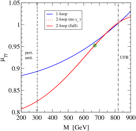
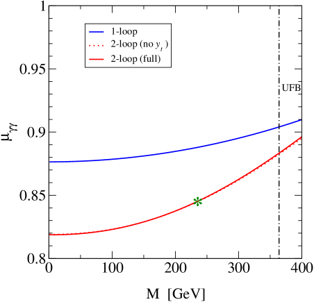
Figure 1: Signal strength for $h\longrightarrow\gamma\gamma$ as a function of $\sqrt{M^{2}}$. The remaining THDM parameters are fixed as in eq. (59) (left plot) or as in eq. (60) (right plot). The meaning of the different lines is explained in the text.

In figure 1 we show the prediction for the signal strength $\mu_{\gamma\gamma}$ as a function of the parameter $M~{}\,\equiv\,\sqrt{M^{2}(M^{2})}$, where the remaining THDM parameters are fixed as in eq. (59) for point A (left plot) or as in eq. (60) for point B (right plot). We do not consider any experimental constraint on the parameter space, although most of them presumably carry over from the analysis of ref. [13] since the BSM Higgs masses and $\tan\beta$ are the same as in the two points introduced there. However, we do implement the theoretical constraints from (tree-level) perturbative unitarity, boundedness from below, and vacuum stability, following eqs. (18)–(28) of ref. [11]. In the region marked as “UFB” on the right of the dot-dashed line in each plot, the quartic Higgs couplings extracted from the tree-level relations between Higgs masses and Lagrangian parameters violate at least one of the conditions for boundedness from below. In the region on the left of the dot-double-dashed line in the left plot, the couplings violate at least one of the conditions for perturbative unitarity of the scattering matrix. In the right plot the unitarity conditions are not violated until $M^{2}\lesssim-(500~{}{\rm GeV})^{2}$, but negative values of $M^{2}$ violate the condition that ensures that the minimum of the potential is a global one.

Coming to the predictions for the signal strength, the solid blue line in each plot represents $\mu_{\gamma\gamma}^{1\ell}$, the solid red line represents our full computation of $\mu_{\gamma\gamma}^{2\ell}$, whereas the dotted red line represents a computation of $\mu_{\gamma\gamma}^{2\ell}$ in which the two-loop BSM contributions controlled by the top Yukawa coupling have been omitted. The green asterisk centered on the solid red line in the left and right plot marks the value of $M$ that corresponds to the point of eqs. (59) and (60), respectively. Since we adopt the limit of vanishing mass for the SM-like Higgs boson, the dependence of the one-loop result on $M$ is given simply by $\mu_{\gamma\gamma}^{1\ell}~{}\approx~{}0.876\,+\,0.12\,x\,+\,0.004\,x^{2}$, where $x=M^{2}/M^{2}_{H^{\pm}}$. Based on this naive estimate of the signal strength, values of $M$ below about $670$ GeV for the left plot and $630$ GeV for the right plot yield a prediction for $\mu_{\gamma\gamma}^{1\ell}$ that, in these scenarios, is more than $2\sigma$ away from the measured value.

The comparison between the blue lines for $\mu_{\gamma\gamma}^{1\ell}$ and the red lines for $\mu_{\gamma\gamma}^{2\ell}$ shows that the two-loop BSM contributions can be significant, especially at lower values of $M$. Being generally negative, they can exacerbate the tension between measurement and theory prediction. Finally, the comparison between the solid and dotted red lines shows that ${\cal P}_{h}^{2\ell,\,{\rm{\scriptscriptstyle BSM}}}$ is largely dominated by the contributions controlled by the quartic Higgs couplings, except for a region at large $M$ in the left plot where those contributions happen to be rather small and are comparable in size with the contributions controlled by the top Yukawa coupling. Once again, figure 1 shows that in the aligned THDM there are scenarios in which a precise determination of $\Gamma[h\rightarrow\gamma\gamma]$ requires the inclusion of the two-loop BSM contributions.

5 Conclusions

The requirement that an extension of the SM accommodate a scalar with properties compatible with those observed at the LHC constrains the parameter space of the BSM model even before the direct observation of any new particles. In models such as the THDM, where some of the couplings in the Lagrangian can take remarkably large values and still be allowed by all theoretical constraints, precise predictions for the properties of the SM-like Higgs boson $h$ and for other EW observables may require that the contributions involving those couplings be accounted for beyond the LO. Following the example of earlier two-loop calculations of the $\rho$ parameter [15, 16], of the scalar mass matrices [17], and of the trilinear self-coupling of the SM-like Higgs boson [18, 19], in this work we computed the two-loop BSM contributions to $\Gamma[h\rightarrow\gamma\gamma]$ in the aligned (and CP-conserving) THDM. In line with the earlier calculations, we adopted the simplifying assumptions of vanishing EW gauge couplings (the so-called “gaugeless limit”) and vanishing mass of the SM-like Higgs boson. The latter assumption allowed us to exploit a LET that connects the $h\gamma\gamma$ amplitude to the derivative of the photon self-energy w.r.t. the Higgs vev. In addition, the alignment and gaugeless limits allowed us to adopt a simplified approach to the renormalization of the mixing in the scalar sector, bypassing the complications related to the possible gauge dependence of the mixing angles that were discussed in refs. [26, 27, 28]. We provided explicit analytic formulas for the two-loop BSM contributions to the photon self-energy. The corresponding formulas for the $h\gamma\gamma$ amplitude can be obtained straightforwardly by exploiting the chain rule for the derivative w.r.t. $v$, and we make them available on request in electronic form.

After describing our calculation, we briefly discussed the numerical impact of the newly-computed two-loop BSM contributions. We chose not to embark in an extensive analysis of the THDM parameter space, but rather focus on two benchmark points introduced in ref. [13], where large values of the quartic Higgs couplings lead to a prediction for the $W$ mass compatible with the recent CDF measurement [14], and $7\sigma$ away from the SM prediction. As expected, such large couplings can also lead to a deviation from the SM prediction for the $h\longrightarrow\gamma\gamma$ decay width. We defined a simplified signal-strength parameter $\mu_{\gamma\gamma}$, and showed how the inclusion of the two-loop BSM contributions can exacerbate the tension between the measured value of the signal strength, which is in fact slightly above the SM prediction, and the prediction of the THDM in the considered benchmark points, which is somewhat below the SM prediction. We also discussed how the prediction for $\mu_{\gamma\gamma}$ depends on the value and, beyond the LO, the definition of the parameter $M^{2}$. In summary, we showed that in the aligned THDM there are scenarios in which the inclusion of the two-loop BSM contributions is required for a precise determination of $\Gamma[h\rightarrow\gamma\gamma]$.

Of course, our discussion of the numerical impact of our results should be viewed as merely qualitative. A detailed study of the constraints on the aligned THDM arising from $\Gamma[h\rightarrow\gamma\gamma]$ would require that we combine the BSM contributions to the $h\gamma\gamma$ amplitude with the most complete determination of the SM contributions, that we account for the BSM corrections to all production and decay processes, that we perform extensive scans over the parameter space of the model, and that we take into account all of the remaining theoretical and experimental constraints. We leave such analysis for future work, hoping that the results presented in this paper will help the collective effort to use the properties of the Higgs boson as a probe of what lies beyond the SM.

Appendix A: One-loop self-energies and tadpoles of the Higgs bosons

In this appendix we list explicit formulas for the one-loop self-energies and tadpoles of the Higgs bosons that are relevant to our calculation. They were obtained by adapting to the THDM the general formulas given in refs. [65, 66], under the limits of alignment, vanishing EW gauge couplings and vanishing SM-like Higgs mass.

$$16\pi^{2}\,\Pi_{H^{+}H^{-}}(m^{2}_{H^{\pm}}) = -\frac{1}{v^{2}}\,\biggr{[}(m^{2}_{H^{\pm}}-m^{2}_{H})^{2}\,B_{0}(m^{2}_{H^{\pm}},m^{2}_{H},0)\,+\,(m^{2}_{H^{\pm}}-m^{2}_{A})^{2}\,B_{0}(m^{2}_{H^{\pm}},m^{2}_{A},0)$$ (A1)

$$~{}~{}~{}~{}~{}~{}~{}+4\,(m^{2}_{H^{\pm}}-M^{2})^{2}\,B_{0}(m^{2}_{H^{\pm}},m^{2}_{H^{\pm}},0)$$

$$~{}~{}~{}~{}~{}~{}~{}-2\,(m^{2}_{H}-M^{2})\cot^{2}2\beta\,\biggr{(}A_{0}(m^{2}_{H})+A_{0}(m^{2}_{A})+4\,A_{0}(m^{2}_{H^{\pm}})$$

$$~{}~{}~{}~{}~{}~{}~{}~{}~{}~{}~{}~{}~{}~{}~{}~{}~{}~{}~{}~{}~{}~{}~{}~{}~{}~{}~{}~{}~{}~{}~{}~{}~{}~{}~{}~{}~{}~{}~{}~{}-2\,(m^{2}_{H}-M^{2})\,B_{0}(m^{2}_{H^{\pm}},m^{2}_{H^{\pm}},m^{2}_{H})\biggr{)}\,\biggr{]}$$

$$- \frac{2\,m_{t}^{2}}{v^{2}}\,N_{c}\,\cot^{2}\beta\,G_{0}(m^{2}_{H^{\pm}},0,m_{t}^{2})~{},$$

$$16\pi^{2}\,\Pi_{hh}(0) = \frac{1}{v^{2}}\,\biggr{[}(m^{2}_{H}-M^{2})\,\biggr{(}A_{0}(m^{2}_{H})-2\,(m^{2}_{H}-M^{2})\,B_{0}(0,m^{2}_{H},m^{2}_{H})\biggr{)}$$ (A2)

$$~{}~{}~{}~{}~{}+\,(m^{2}_{A}-M^{2})\,\biggr{(}A_{0}(m^{2}_{A})-2\,(m^{2}_{A}-M^{2})\,B_{0}(0,m^{2}_{A},m^{2}_{A})\biggr{)}$$

$$~{}~{}~{}~{}~{}+\,2\,(m^{2}_{H^{\pm}}-M^{2})\,\biggr{(}A_{0}(m^{2}_{H^{\pm}})-2\,(m^{2}_{H^{\pm}}-M^{2})\,B_{0}(0,m^{2}_{H^{\pm}},m^{2}_{H^{\pm}})\biggr{)}\biggr{]}$$

$$+ \frac{2\,m_{t}^{2}}{v^{2}}\,N_{c}\,\biggr{(}2\,m_{t}^{2}\,B_{0}(0,m_{t}^{2},m_{t}^{2})-G_{0}(0,m_{t}^{2},m_{t}^{2})\biggr{)}~{},$$

$$16\pi^{2}\,\Pi_{hH}(0) = \frac{M^{2}-m^{2}_{H}}{v^{2}}\,\cot 2\beta\,\biggr{[}3\,\biggr{(}A_{0}(m^{2}_{H})-2\,(m^{2}_{H}-M^{2})\,B_{0}(0,m^{2}_{H},m^{2}_{H})\biggr{)}$$ (A3)

$$~{}~{}~{}~{}~{}~{}~{}~{}~{}~{}~{}~{}~{}~{}~{}~{}~{}~{}~{}~{}~{}~{}~{}~{}+\,A_{0}(m^{2}_{A})-2\,(m^{2}_{A}-M^{2})\,B_{0}(0,m^{2}_{A},m^{2}_{A})$$

$$~{}~{}~{}~{}~{}~{}~{}~{}~{}~{}~{}~{}~{}~{}~{}~{}~{}~{}~{}~{}~{}~{}~{}\,+\,2\,\biggr{(}A_{0}(m^{2}_{H^{\pm}})-2\,(m^{2}_{H^{\pm}}-M^{2})\,B_{0}(0,m^{2}_{H^{\pm}},m^{2}_{H^{\pm}})\biggr{)}\biggr{]}$$

$$- \frac{2\,m_{t}^{2}}{v^{2}}\,N_{c}\,\cot\beta\,\biggr{(}2\,m_{t}^{2}\,B_{0}(0,m_{t}^{2},m_{t}^{2})-G_{0}(0,m_{t}^{2},m_{t}^{2})\biggr{)}~{},$$

$$16\pi^{2}\,T_{h} = \frac{1}{v}\,\biggr{[}(m^{2}_{H}-M^{2})\,A_{0}(m^{2}_{H})\,+\,(m^{2}_{A}-M^{2})\,A_{0}(m^{2}_{A})\,+\,2\,(m^{2}_{H^{\pm}}-M^{2})\,A_{0}(m^{2}_{H^{\pm}})\biggr{]}$$ (A4)

$$- \frac{4\,m_{t}^{2}}{v}\,N_{c}\,A_{0}(m_{t}^{2})~{},$$

$$16\pi^{2}\,T_{H} = \frac{M^{2}-m^{2}_{H}}{v}\,\cot 2\beta\,\biggr{[}3\,A_{0}(m^{2}_{H})\,+\,A_{0}(m^{2}_{A})\,+\,2\,A_{0}(m^{2}_{H^{\pm}})\biggr{]}$$ (A5)

$$+ \frac{4\,m_{t}^{2}}{v}\,N_{c}\,\cot\beta\,A_{0}(m_{t}^{2})~{},$$

where

$$G_{0}(p^{2},m_{1}^{2},m_{2}^{2})~{}=~{}(p^{2}-m_{1}^{2}-m_{2}^{2})\,B_{0}(p^{2},m_{1}^{2},m_{2}^{2})+A_{0}(m_{1}^{2})+A_{0}(m_{2}^{2})~{},$$ (A6)

and

$$A_{0}(m^{2}) = m^{2}\,\left(\ln\frac{m^{2}}{Q^{2}}-1\right)~{},$$ (A7)

$$B_{0}(0,m^{2},m^{2}) = -\ln\frac{m^{2}}{Q^{2}}~{},$$ (A8)

$${\rm Re}\,B_{0}(p^{2},0,m^{2})\,=\,{\rm Re}\,B_{0}(p^{2},m^{2},0) = 2\,-\,\ln\frac{m^{2}}{Q^{2}}\,-\,\left(1-\frac{m^{2}}{p^{2}}\right)\,\ln\left|1-\frac{p^{2}}{m^{2}}\right|.$$ (A9)

For the function $B_{0}(m^{2}_{H^{\pm}},m^{2}_{H^{\pm}},m^{2}_{H})$ in eq. (A1) we used the code LoopTools [67]. We checked that our result for the charged-Higgs self-energy agrees with the corresponding result in ref. [19].

Appendix B: Two-loop self-energy of the photon

Under the assumptions of alignment, vanishing EW gauge couplings, and vanishing SM-like Higgs mass, the BSM part of the two-loop self-energy of the photon reads

$$\Pi_{\gamma\gamma}^{2\ell,\,{\rm{\scriptscriptstyle BSM}}}(0) = \frac{\alpha}{48\pi^{3}v^{2}}\,\biggr{[}~{}(m^{2}_{H^{\pm}}-M^{2})^{2}\,F_{h}(m^{2}_{H^{\pm}})$$ (B1)

$$~{}~{}~{}~{}~{}~{}~{}~{}~{}~{}~{}+\,\frac{(m^{2}_{H}-m^{2}_{H^{\pm}})^{2}}{4}\,F_{G}(m^{2}_{H},m^{2}_{H^{\pm}})$$

$$~{}~{}~{}~{}~{}~{}~{}~{}~{}~{}~{}+\,\frac{(m^{2}_{A}-m^{2}_{H^{\pm}})^{2}}{4}\,F_{G}(m^{2}_{A},m^{2}_{H^{\pm}})$$

$$~{}~{}~{}~{}~{}~{}~{}~{}~{}~{}~{}+\,(m^{2}_{H}-M^{2})^{2}\,\cot^{2}2\beta\,F_{H}(m^{2}_{H},m^{2}_{H^{\pm}})$$

$$~{}~{}~{}~{}~{}~{}~{}~{}~{}~{}~{}+\,\frac{m^{2}_{H}-M^{2}}{2\,m^{2}_{H^{\pm}}}\,\cot^{2}2\beta\,\biggr{(}A_{0}(m^{2}_{H})\,+\,A_{0}(m^{2}_{A})\,+4\,\,A_{0}(m^{2}_{H^{\pm}})\biggr{)}$$

$$~{}~{}~{}~{}~{}~{}~{}~{}~{}~{}~{}+m_{t}^{2}\,\cot^{2}\beta\,N_{c}\,\biggr{(}f_{H}(m_{t}^{2}/m^{2}_{H})\,+\,f_{A}(m_{t}^{2}/m^{2}_{A})\,+\,f_{H^{\pm}}(m_{t}^{2}/m^{2}_{H^{\pm}})$$

$$~{}~{}~{}~{}~{}~{}~{}~{}~{}~{}~{}~{}~{}~{}~{}~{}~{}~{}~{}~{}~{}~{}~{}~{}~{}~{}~{}~{}~{}~{}~{}~{}~{}~{}~{}-\frac{A_{0}(m_{t}^{2})}{m^{2}_{H^{\pm}}}\,-\,\frac{43}{72}\,-\,\frac{1}{3}\,\ln\frac{m_{t}^{2}}{Q^{2}}\,\biggr{)}\biggr{]}~{},$$

where we also assume that the one-loop part of the photon self-energy, see eq. (40), is expressed in terms of $\overline{\rm MS}$-renormalized masses, and in particular the charged-Higgs contribution is expressed in terms of the parameter $\widehat{m}^{2}_{H^{\pm}}$ defined in eq. (32). If the one-loop part was instead expressed in terms of the parameter $\widetilde{m}^{2}_{H^{\pm}}$ defined in eq. (33), $\Pi_{\gamma\gamma}^{2\ell,\,{\rm{\scriptscriptstyle BSM}}}(0)$ would receive an additional contribution corresponding to the second term within parentheses in eq. (46).

The function $A_{0}(m^{2})$ entering eq. (B1) is defined in eq. (A7), and the remaining functions are

$$F_{h}(m^{2})~{}=~{}\frac{1}{m^{2}}\left(\ln\frac{m^{2}}{Q^{2}}-\frac{1}{2}\right)~{},$$ (B2)

$$F_{G}(m_{1}^{2},m_{2}^{2})~{}=~{}\frac{1}{m_{2}^{2}}\left(\ln\frac{m_{1}^{2}}{Q^{2}}-1\right)\,-\,\frac{2\,(4\,m_{1}^{2}+5\,m_{2}^{2})}{(m_{1}^{2}-m_{2}^{2})^{2}}\,+\,\frac{m_{2}^{2}\,(17\,m_{1}^{2}+m_{2}^{2})}{(m_{1}^{2}-m_{2}^{2})^{3}}\,\ln\frac{m_{1}^{2}}{m_{2}^{2}}~{},$$ (B3)

$$F_{H}(m_{1}^{2},m_{2}^{2})~{}=~{}\frac{1}{m_{2}^{2}}\left(\ln\frac{m_{1}^{2}}{Q^{2}}-1\right)\,+\,\frac{1}{m_{1}^{2}-4\,m_{2}^{2}}\,+\,\frac{m_{1}^{2}-10\,m_{2}^{2}}{(m_{1}^{2}-4\,m_{2}^{2})^{2}}\,\ln\frac{m_{1}^{2}}{m_{2}^{2}}\,+\,\frac{6\,m_{2}^{4}}{m_{1}^{2}\,(m_{1}^{2}-4\,m_{2}^{2})^{2}}\,\phi\left(\frac{m_{1}^{2}}{4\,m_{2}^{2}}\right)~{},$$ (B4)

$$f_{H}(x)~{}=~{}\frac{-2}{3\,(1-4\,x)}\,\left[(1+2\,x)\ln x\,+\,2\,x\,(1-x)\,\phi(\frac{1}{4x})\right]~{},$$ (B5)

$$f_{A}(x)~{}=~{}\frac{2}{9\,(1-4\,x)^{2}}\,\left[1\,-\,4\,x\,+\,(5-14\,x)\ln x\,+\,6\,x\,(1-3\,x)\,\phi(\frac{1}{4x})\right]~{},$$ (B6)

$$f_{H^{\pm}}(x)~{}=~{}-\frac{\ln x}{9\,(1-x)}~{}.$$ (B7)

The function $\phi(z)$ entering eqs. (B4)–(B6) is defined as

$$\phi(z)=\left\{\begin{tabular}[]{ll}$4\,\sqrt{\frac{z}{1-z}}~{}{\rm Cl}_{2}(2\arcsin\sqrt{z})$ \, ,&$(0<z<1)$ \, ,\\ \\ ${\frac{1}{\lambda}\left[-4\,{\rm Li_{2}}(\frac{1-\lambda}{2})+2\,\ln^{2}(\frac{1-\lambda}{2})-\ln^{2}(4z)+\pi^{2}/3\right]}$ \, ,&~{}~{}~{}$(z\geq 1)$ \,,\end{tabular}\right.$$ (B8)

where ${\rm Cl}_{2}(z)={\rm Im}\,{\rm Li_{2}}(e^{iz})$ is the Clausen function, and $\lambda=\sqrt{1-(1/z)}$. A recursive relation for the derivative of $\phi(z)$,

$$\frac{d}{dz}\,\phi(z)~{}=~{}\frac{2}{z-1}\,\left(\ln 4z-\frac{\phi(z)}{4z}\right)~{},$$ (B9)

proves very useful in obtaining compact results for the derivatives of $\Pi_{\gamma\gamma}^{2\ell,\,{\rm{\scriptscriptstyle BSM}}}(0)$ w.r.t. the masses of the top quark and of the BSM Higgs bosons, see eq. (41).

References

- [1] CMS Collaboration, S. Chatrchyan et al., Observation of a New Boson at a Mass of 125 GeV with the CMS Experiment at the LHC. Phys. Lett. B 716 (2012) 30–61, arXiv:1207.7235 [hep-ex].
- [2] ATLAS Collaboration, G. Aad et al., Observation of a new particle in the search for the Standard Model Higgs boson with the ATLAS detector at the LHC. Phys. Lett. B 716 (2012) 1–29, arXiv:1207.7214 [hep-ex].
- [3] ATLAS, CMS Collaboration, G. Aad et al., Combined Measurement of the Higgs Boson Mass in Collisions at and 8 TeV with the ATLAS and CMS Experiments. Phys. Rev. Lett. 114 (2015) 191803, arXiv:1503.07589 [hep-ex].
- [4] ATLAS, CMS Collaboration, G. Aad et al., Measurements of the Higgs boson production and decay rates and constraints on its couplings from a combined ATLAS and CMS analysis of the LHC pp collision data at and 8 TeV. JHEP 08 (2016) 045, arXiv:1606.02266 [hep-ex].
- [5] J. F. Gunion, H. E. Haber, G. L. Kane, and S. Dawson, The Higgs Hunter’s Guide. Front. Phys. 80 (2000) .
- [6] M. Aoki, S. Kanemura, K. Tsumura, and K. Yagyu, Models of Yukawa interaction in the two Higgs doublet model, and their collider phenomenology. Phys. Rev. D 80 (2009) 015017, arXiv:0902.4665 [hep-ph].
- [7] G. C. Branco, P. M. Ferreira, L. Lavoura, M. N. Rebelo, M. Sher, and J. P. Silva, Theory and phenomenology of two-Higgs-doublet models. Phys. Rept. 516 (2012) 1–102, arXiv:1106.0034 [hep-ph].
- [8] J. F. Gunion and H. E. Haber, The CP conserving two Higgs doublet model: The Approach to the decoupling limit. Phys. Rev. D 67 (2003) 075019, arXiv:hep-ph/0207010.
- [9] I. Antoniadis, K. Benakli, A. Delgado, and M. Quiros, A New gauge mediation theory. Adv. Stud. Theor. Phys. 2 (2008) 645–672, arXiv:hep-ph/0610265.
- [10] M. Carena, I. Low, N. R. Shah, and C. E. M. Wagner, Impersonating the Standard Model Higgs Boson: Alignment without Decoupling. JHEP 04 (2014) 015, arXiv:1310.2248 [hep-ph].
- [11] F. Arco, S. Heinemeyer, and M. J. Herrero, Exploring sizable triple Higgs couplings in the 2HDM. Eur. Phys. J. C 80 (2020) no. 9, 884, arXiv:2005.10576 [hep-ph].
- [12] F. Arco, S. Heinemeyer, and M. J. Herrero, Triple Higgs couplings in the 2HDM: the complete picture. Eur. Phys. J. C 82 (2022) no. 6, 536, arXiv:2203.12684 [hep-ph].
- [13] H. Bahl, J. Braathen, and G. Weiglein, New physics effects on the W-boson mass from a doublet extension of the SM Higgs sector. Phys. Lett. B 833 (2022) 137295, arXiv:2204.05269 [hep-ph].
- [14] CDF Collaboration, T. Aaltonen et al., High-precision measurement of the boson mass with the CDF II detector. Science 376 (2022) no. 6589, 170–176.
- [15] S. Hessenberger and W. Hollik, Two-loop corrections to the parameter in Two-Higgs-Doublet Models. Eur. Phys. J. C 77 (2017) no. 3, 178, arXiv:1607.04610 [hep-ph].
- [16] S. Hessenberger and W. Hollik, Two-loop improved predictions for and in Two-Higgs-Doublet models. Eur. Phys. J. C 82 (2022) no. 10, 970, arXiv:2207.03845 [hep-ph].
- [17] J. Braathen, M. D. Goodsell, and F. Staub, Supersymmetric and non-supersymmetric models without catastrophic Goldstone bosons. Eur. Phys. J. C 77 (2017) no. 11, 757, arXiv:1706.05372 [hep-ph].
- [18] J. Braathen and S. Kanemura, On two-loop corrections to the Higgs trilinear coupling in models with extended scalar sectors. Phys. Lett. B 796 (2019) 38–46, arXiv:1903.05417 [hep-ph].
- [19] J. Braathen and S. Kanemura, Leading two-loop corrections to the Higgs boson self-couplings in models with extended scalar sectors. Eur. Phys. J. C 80 (2020) no. 3, 227, arXiv:1911.11507 [hep-ph].
- [20] Particle Data Group Collaboration, R. L. Workman et al., Review of Particle Physics. PTEP 2022 (2022) 083C01.
- [21] F. Arco, S. Heinemeyer, and M. J. Herrero, Sensitivity and constraints to the 2HDM soft-breaking parameter . Phys. Lett. B 835 (2022) 137548, arXiv:2207.13501 [hep-ph].
- [22] M. A. Shifman, A. I. Vainshtein, M. B. Voloshin, and V. I. Zakharov, Low-Energy Theorems for Higgs Boson Couplings to Photons. Sov. J. Nucl. Phys. 30 (1979) 711–716.
- [23] B. A. Kniehl and M. Spira, Low-energy theorems in Higgs physics. Z. Phys. C 69 (1995) 77–88, arXiv:hep-ph/9505225.
- [24] S. Davidson and H. E. Haber, Basis-independent methods for the two-Higgs-doublet model. Phys. Rev. D 72 (2005) 035004, arXiv:hep-ph/0504050. [Erratum: Phys.Rev.D 72, 099902 (2005)].
- [25] S. Kanemura, Y. Okada, E. Senaha, and C. P. Yuan, Higgs coupling constants as a probe of new physics. Phys. Rev. D 70 (2004) 115002, arXiv:hep-ph/0408364.
- [26] M. Krause, R. Lorenz, M. Muhlleitner, R. Santos, and H. Ziesche, Gauge-independent Renormalization of the 2-Higgs-Doublet Model. JHEP 09 (2016) 143, arXiv:1605.04853 [hep-ph].
- [27] L. Altenkamp, S. Dittmaier, and H. Rzehak, Renormalization schemes for the Two-Higgs-Doublet Model and applications to h fermions. JHEP 09 (2017) 134, arXiv:1704.02645 [hep-ph].
- [28] S. Kanemura, M. Kikuchi, K. Sakurai, and K. Yagyu, Gauge invariant one-loop corrections to Higgs boson couplings in non-minimal Higgs models. Phys. Rev. D 96 (2017) no. 3, 035014, arXiv:1705.05399 [hep-ph].
- [29] H.-Q. Zheng and D.-D. Wu, First order QCD corrections to the decay of the Higgs boson into two photons. Phys. Rev. D 42 (1990) 3760–3763.
- [30] A. Djouadi, M. Spira, J. J. van der Bij, and P. M. Zerwas, QCD corrections to gamma gamma decays of Higgs particles in the intermediate mass range. Phys. Lett. B 257 (1991) 187–190.
- [31] S. Dawson and R. P. Kauffman, QCD corrections to H — gamma gamma. Phys. Rev. D 47 (1993) 1264–1267.
- [32] K. Melnikov and O. I. Yakovlev, Higgs — two photon decay: QCD radiative correction. Phys. Lett. B 312 (1993) 179–183, arXiv:hep-ph/9302281.
- [33] A. Djouadi, M. Spira, and P. M. Zerwas, Two photon decay widths of Higgs particles. Phys. Lett. B 311 (1993) 255–260, arXiv:hep-ph/9305335.
- [34] M. Inoue, R. Najima, T. Oka, and J. Saito, QCD corrections to two photon decay of the Higgs boson and its reverse process. Mod. Phys. Lett. A 9 (1994) 1189–1194.
- [35] J. Fleischer, O. V. Tarasov, and V. O. Tarasov, Analytical result for the two loop QCD correction to the decay H — 2 gamma. Phys. Lett. B 584 (2004) 294–297, arXiv:hep-ph/0401090.
- [36] Y. Liao and X.-y. Li, O (alpha**2 G(F)m(t)**2) contributions to H — gamma gamma. Phys. Lett. B 396 (1997) 225–230, arXiv:hep-ph/9605310.
- [37] A. Djouadi, P. Gambino, and B. A. Kniehl, Two loop electroweak heavy fermion corrections to Higgs boson production and decay. Nucl. Phys. B 523 (1998) 17–39, arXiv:hep-ph/9712330.
- [38] F. Fugel, B. A. Kniehl, and M. Steinhauser, Two loop electroweak correction of O(G(F)M(t)**2) to the Higgs-boson decay into photons. Nucl. Phys. B 702 (2004) 333–345, arXiv:hep-ph/0405232.
- [39] G. Degrassi and F. Maltoni, Two-loop electroweak corrections to the Higgs-boson decay H — gamma gamma. Nucl. Phys. B 724 (2005) 183–196, arXiv:hep-ph/0504137.
- [40] U. Aglietti, R. Bonciani, G. Degrassi, and A. Vicini, Two loop light fermion contribution to Higgs production and decays. Phys. Lett. B 595 (2004) 432–441, arXiv:hep-ph/0404071.
- [41] U. Aglietti, R. Bonciani, G. Degrassi, and A. Vicini, Master integrals for the two-loop light fermion contributions to gg — H and H — gamma gamma. Phys. Lett. B 600 (2004) 57–64, arXiv:hep-ph/0407162.
- [42] G. Passarino, C. Sturm, and S. Uccirati, Complete Two-Loop Corrections to H — gamma gamma. Phys. Lett. B 655 (2007) 298–306, arXiv:0707.1401 [hep-ph].
- [43] S. Actis, G. Passarino, C. Sturm, and S. Uccirati, NNLO Computational Techniques: The Cases H — gamma gamma and H — g g. Nucl. Phys. B 811 (2009) 182–273, arXiv:0809.3667 [hep-ph].
- [44] T. Hahn, Generating Feynman diagrams and amplitudes with FeynArts 3. Comput. Phys. Commun. 140 (2001) 418–431, arXiv:hep-ph/0012260.
- [45] A. I. Davydychev and J. B. Tausk, Two loop selfenergy diagrams with different masses and the momentum expansion. Nucl. Phys. B 397 (1993) 123–142.
- [46] G. Degrassi and P. Slavich, NLO QCD bottom corrections to Higgs boson production in the MSSM. JHEP 11 (2010) 044, arXiv:1007.3465 [hep-ph].
- [47] F. Staub, SARAH. arXiv:0806.0538 [hep-ph].
- [48] F. Staub, From Superpotential to Model Files for FeynArts and CalcHep/CompHep. Comput. Phys. Commun. 181 (2010) 1077–1086, arXiv:0909.2863 [hep-ph].
- [49] F. Staub, Automatic Calculation of supersymmetric Renormalization Group Equations and Self Energies. Comput. Phys. Commun. 182 (2011) 808–833, arXiv:1002.0840 [hep-ph].
- [50] F. Staub, SARAH 3.2: Dirac Gauginos, UFO output, and more. Comput. Phys. Commun. 184 (2013) 1792–1809, arXiv:1207.0906 [hep-ph].
- [51] F. Staub, SARAH 4 : A tool for (not only SUSY) model builders. Comput. Phys. Commun. 185 (2014) 1773–1790, arXiv:1309.7223 [hep-ph].
- [52] P. S. Bhupal Dev and A. Pilaftsis, Maximally Symmetric Two Higgs Doublet Model with Natural Standard Model Alignment. JHEP 12 (2014) 024, arXiv:1408.3405 [hep-ph]. [Erratum: JHEP 11, 147 (2015)].
- [53] A. Barroso, P. M. Ferreira, I. P. Ivanov, and R. Santos, Metastability bounds on the two Higgs doublet model. JHEP 06 (2013) 045, arXiv:1303.5098 [hep-ph].
- [54] B. Grinstein, C. W. Murphy, and P. Uttayarat, One-loop corrections to the perturbative unitarity bounds in the CP-conserving two-Higgs doublet model with a softly broken symmetry. JHEP 06 (2016) 070, arXiv:1512.04567 [hep-ph].
- [55] V. Cacchio, D. Chowdhury, O. Eberhardt, and C. W. Murphy, Next-to-leading order unitarity fits in Two-Higgs-Doublet models with soft breaking. JHEP 11 (2016) 026, arXiv:1609.01290 [hep-ph].
- [56] P. Bechtle, S. Heinemeyer, O. Stål, T. Stefaniak, and G. Weiglein, : Confronting arbitrary Higgs sectors with measurements at the Tevatron and the LHC. Eur. Phys. J. C 74 (2014) no. 2, 2711, arXiv:1305.1933 [hep-ph].
- [57] P. Bechtle, S. Heinemeyer, T. Klingl, T. Stefaniak, G. Weiglein, and J. Wittbrodt, HiggsSignals-2: Probing new physics with precision Higgs measurements in the LHC 13 TeV era. Eur. Phys. J. C 81 (2021) no. 2, 145, arXiv:2012.09197 [hep-ph].
- [58] P. Bechtle, O. Brein, S. Heinemeyer, G. Weiglein, and K. E. Williams, HiggsBounds: Confronting Arbitrary Higgs Sectors with Exclusion Bounds from LEP and the Tevatron. Comput. Phys. Commun. 181 (2010) 138–167, arXiv:0811.4169 [hep-ph].
- [59] P. Bechtle, O. Brein, S. Heinemeyer, G. Weiglein, and K. E. Williams, HiggsBounds 2.0.0: Confronting Neutral and Charged Higgs Sector Predictions with Exclusion Bounds from LEP and the Tevatron. Comput. Phys. Commun. 182 (2011) 2605–2631, arXiv:1102.1898 [hep-ph].
- [60] P. Bechtle, O. Brein, S. Heinemeyer, O. Stål, T. Stefaniak, G. Weiglein, and K. E. Williams, : Improved Tests of Extended Higgs Sectors against Exclusion Bounds from LEP, the Tevatron and the LHC. Eur. Phys. J. C 74 (2014) no. 3, 2693, arXiv:1311.0055 [hep-ph].
- [61] P. Bechtle, D. Dercks, S. Heinemeyer, T. Klingl, T. Stefaniak, G. Weiglein, and J. Wittbrodt, HiggsBounds-5: Testing Higgs Sectors in the LHC 13 TeV Era. Eur. Phys. J. C 80 (2020) no. 12, 1211, arXiv:2006.06007 [hep-ph].
- [62] H. Bahl, V. M. Lozano, T. Stefaniak, and J. Wittbrodt, Testing exotic scalars with HiggsBounds. Eur. Phys. J. C 82 (2022) no. 7, 584, arXiv:2109.10366 [hep-ph].
- [63] J. Haller, A. Hoecker, R. Kogler, K. Mönig, T. Peiffer, and J. Stelzer, Update of the global electroweak fit and constraints on two-Higgs-doublet models. Eur. Phys. J. C 78 (2018) no. 8, 675, arXiv:1803.01853 [hep-ph].
- [64] M. Aiko, J. Braathen, and S. Kanemura, Leading two-loop corrections to the Higgs di-photon decay in the Inert Doublet Model. arXiv:2307.14976 [hep-ph].
- [65] J. Braathen and M. D. Goodsell, Avoiding the Goldstone Boson Catastrophe in general renormalisable field theories at two loops. JHEP 12 (2016) 056, arXiv:1609.06977 [hep-ph].
- [66] J. Braathen, M. D. Goodsell, and P. Slavich, Matching renormalisable couplings: simple schemes and a plot. Eur. Phys. J. C 79 (2019) no. 8, 669, arXiv:1810.09388 [hep-ph].
- [67] T. Hahn and M. Perez-Victoria, Automatized one loop calculations in four-dimensions and D-dimensions. Comput. Phys. Commun. 118 (1999) 153–165, arXiv:hep-ph/9807565.